Move Complexity of a Self-Stabilizing Algorithm for Maximal Independent Sets
Institute of Telematics
Hamburg University of Technology
21073 Hamburg, Germany
turau@tuhh.de
Abstract
is a self-stabilizing algorithm that computes a maximal independent set in a finite graph with approximation ratio . In this note we show that under the central scheduler the number of moves of is not bounded by a polynomial in .
Keywords Self-stabilizing Algorithm, Maximal Independent Sets, Complexity
1 Introduction
There exist several self-stabilizing algorithms to compute a maximal independent set in a finite graph [1, 2, 3, 4, 5]. Algorithm proposed by Yen et al. is especial because it is the only one with a guaranteed approximation ratio. In Theorem 3.13 of [5] the authors prove that the approximation ratio of is . The authors also prove that the algorithm stabilizes for every graph, but an upper bound for the move complexity was not given. In this note we show that for some graphs the move complexity grows exponentially with the size of the graph.
2 Algorithm
Let be an undirected finite graph. For denote by the set of neighbors of and let . The degree of a node equals . Let and denote by the set of neighbors of with degree at most that of .
Algorithm uses a single variable for each node. This variable can have the values and . Let . consists of the following two simple rules:
-
R1:
-
R2:
stabilizes under the central scheduler and if no rule is enabled the set is a maximal independent set of [5]. For regular graphs, algorithm coincides with the algorithm proposed in [2]. Algorithm preferentially places nodes with smaller degree into state . The intention is to find larger independent sets. The following theorem is proved in [5].
Theorem 1.
has approximation ratio of is .
3 Construction of Graphs
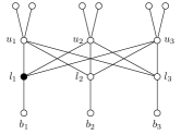
In this section we construct a family of graphs for which requires an exponentially growing number of moves. The construction of depends on two parameters and . Let be a complete bipartite graph with nodes. The nodes of consist of the two independent sets, the upper nodes and the lower nodes . The graph basically consists of of copies of . These graphs are arranged vertically and adjacent copies are connected by edges: one edge between each node of one copy of and node of the copy below. Furthermore, we attach to each node of the lowest copy of a node . So far we nodes. Each node of any of the copies of has degree . Next we attach more leaves to the nodes of the subgraphs . The goal of this last step is to attain a graph, where the degree of a node is one less than the degrees of the neighbors that are one level higher. Fig. 1 shows the graph . Note that and .
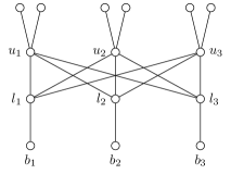
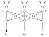
The number of nodes attached in the last step is equal to
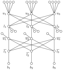
Thus, graph has nodes and . Fig. 2 shows the graph .
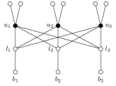
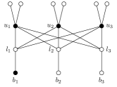
4 Executing on
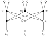
First we consider the graph . We start with an initial configuration where each node is in state (see Fig. 3). In the first steps all execute rule R1 and change to state . Then node also changes to state , note that . This enables rule R2 for all nodes and one by one changes back to state . Then node also executes rule R1 and changes to . This forces node to change back to state . Now we are back at the initial configuration, except for node which is now in state . Next the described process repeats itself, with (resp. ) assuming the role of (resp. ). Then we are back again in the initial configuration except for nodes and . This sequence repeats itself times resulting in a configuration where all nodes but are in state . In this execution rule R1 was executed at least times.

Next we consider the graph (see Fig. 2). We start again with an initial configuration where each node is in state . We can repeat the execution described for graph for the upper copy of the bipartite graph with the only difference the nodes of the lower copy of take over the role of the nodes . To avoid confusion we denote the nodes of this copy of by and . Thus, we reach a configuration where all nodes but nodes are in state . At this point in time rule R1 has been executed at least times. Then node changes to state . This forces all nodes to change back to . Then node also executes rule R1 and changes to . This forces node to change back to state . Now we are back at the initial configuration, except for node which is now in state . Then the whole process beginning with the upper copy of repeats again. This time nodes and take over the role of and . Thus, so far rule R1 has been executed at least times. We can repeat the process times. Thus, there exists an execution of for that contains at least executions of rule R1.
This construction also works for graphs for any value of . Hence, there is an execution of for that contains at least moves. Let and . Then . Thus, there exist a graph with nodes for which requires moves.
Theorem 2.
Using the central scheduler the number of moves of algorithm is not bounded by a polynomial in .
References
- [1] Michiyo Ikeda, Sayaka Kamei, and Hirotsugu Kakugawa. A space-optimal self-stabilizing algorithm for the maximal independent set problem. In the Third International Conference on Parallel and Distributed Computing, Applications and Technologies (PDCAT), pages 70–74, 2002.
- [2] S.M. Hedetniemi, S.T. Hedetniemi, D.P. Jacobs, and P.K. Srimani. Self-stabilizing algorithms for minimal dominating sets and maximal independent sets. Computer Mathematics and Applications, 46(5-6):805–811, 2003.
- [3] Volker Turau. Linear self-stabilizing algorithms for the independent and dominating set problems using an unfair distributed scheduler. Information Processing Letters., 103(3):88–93, July 2007.
- [4] Well Y. Chiu, Chiuyuan Chen, and Shih-Yu Tsai. A 4n-move self-stabilizing algorithm for the minimal dominating set problem using an unfair distributed daemon. Information Processing Letters, 114(10):515 – 518, 2014.
- [5] Li-Hsing Yen, Jean-Yao Huang, and Volker Turau. Designing self-stabilizing systems using game theory. ACM Transactions on Autonomous and Adaptive Systems, Volume 11, Issue 3, Article 18:1–27, 2016.