Nonlinear damped spatially periodic breathers and the emergence of soliton-like rogue waves

Abstract

The spatially periodic breather solutions (SPBs) of the nonlinear Schrödinger equation, prominent in modeling rogue waves, are unstable. In this paper we numerically investigate the routes to stability of the SPBs and related rogue wave activity in the framework of the nonlinear damped higher order nonlinear Schrödinger (NLD-HONLS) equation. The NLD-HONLS solutions are initialized with single-mode and two-mode SPB data at different stages of their development. The Floquet spectral theory of the NLS equation is applied to interpret and provide a characterization of the perturbed dynamics in terms of nearby solutions of the NLS equation. A broad categorization of the routes to stability of the SPBs is determined. Novel behavior related to the effects of nonlinear damping is obtained: tiny bands of complex spectrum develop in the Floquet decomposition of the NLD-HONLS data, indicating the breakup of the SPB into either a one or two “soliton-like” structure. For solutions initialized in the early to middle stage of the development of the modulational instability, we find that all the rogue waves in the NLD-HONLS flow occur when the spectrum is in a one or two soliton-like configuration. When the solutions are initialized as the modulational instability is saturating, rogue waves may occur when the spectrum is not in a soliton-like state. Another distinctive feature of the nonlinear damped dynamics is that the growth of instabilities can be delayed and expressed at higher order due to permanent frequency downshifting

1 Introduction

The nonlinear Schrödinger (NLS) equation arises in many fields when modeling phenomena in which modulational instability (MI) and nonlinear focusing are important. In particular, the NLS equation has proven very useful for initiating studies of rogue waves in deep water. The heteroclinic orbits of modulationally unstable Stokes waves, also termed spatially periodic breathers (SPBs), are large amplitude solutions of the NLS equation which capture the salient features of rogue waves and have come to be regarded as prototypes of deep water rogue waves [1, 2, 3, 4]. More recently, heteroclinic orbits of unstable $N$-phase solutions have been proposed as models of rogue waves over non-uniform backgrounds [5, 6, 7].

The details of the MI for spatially $L$-periodic solutions of the NLS equation depend on, amongst other things, the amplitude of the background and the size $L$ of the domain. For the Stokes wave of fixed amplitude $a$ and $L>L_{0}$ (the threshold for instability), as $L$ increases the number of unstable modes (UMs) increases. In the case of the Stokes wave with $N$ UMs, the associated SPBs can have $M\leq N$ modes active and are referred to as $M$-mode SPBs (the single mode SPB is the Akhmediev breather). Given their prominence in modeling rogue wave phenomena, the stability of the SPBs is important. The squared eigenfunction connection between the nonlinear spectrum of the NLS equation and the linear stability problem was successfully used to establish the linear instability of the $M$-mode SPBs ($M<N$) [8]. The exact nature of the instability of the special “maximal” SPBs (when $M=N$) is currently under investigation [12].

An important phenomenon related to MI is frequency downshifting which occurs when the energy transfer from the carrier wave to a lower sideband becomes permanent. For sufficiently steep waves, frequency downshifting has been observed in both laboratory experiments and in ocean waves and it was noted that dissipation is most likely essential for permanent downshift of a realistic wave spectrum [16, 17]. More realistic explorations of deep water wave dynamics can be achieved with the Dysthe equation which accurately predicts laboratory data for a wider range of wave parameters than the NLS equation [13, 14, 15]. Even so, frequency downshifting is not captured by either the linear damped NLS or Dysthe equations as the momentum and energy decay at the same rate, thus preserving the spectral center. Permanent downshifting is captured by a nonlinear damped higher order nonlinear Schrödinger (NLD-HONLS) equation:

$$iu_{t}+u_{xx}+2|u|^{2}u+i\epsilon\left(\mbox{$\frac{1}{2}$}u_{xxx}-8|u|^{2}u_{x}-2ui(1+i\beta)\left[\mathcal{H}\left(|u|^{2}\right)\right]_{x}\right)=0,$$ (1)

where $0<\epsilon,\beta<<1$, $u(x,t)$ is the complex envelope of the wave train and is $L$-periodic in space. Here $\mathcal{H}\{f(x)\}=\frac{1}{\pi}\int_{-\infty}^{\infty}\frac{f(\xi)}{x-\xi}d\xi$ is the Hilbert transform of $f$. In a comparative study, it was shown to be one of the most accurate models for predicting the permanent downshift observed in a set of laboratory experiments [18, 14].

In this article we investigate the routes to stability of single-mode and multi-mode SPBs over an unstable Stokes wave background and related rogue wave activity in the framework of the NLD-HONLS equation. The initial data used in the numerical experiments is generated by evaluating exact one or two mode SPB solutions of the integrable NLS equation at time $T_{0}$, i.e. $U^{(j)}(x,T_{0})$ or $U^{(i,j)}(x,T_{0})$ (see Equations (8)-(9)). We systematically vary $T_{0}\in[-5,0]$ to allow the NLD-HONLS solutions to be initialized with SPB data at different stages of their development, i.e. from the early stage of the MI when there is strong growth ($T_{0}=-5$) through the nonlinear stage when the MI is saturating ($T_{0}=0$).

Viewing the NLD-HONLS dynamics as near integrable, the perturbed flow is analyzed by appealing to the Floquet spectral theory of the NLS equation. This type of normal mode analysis, where a characterization of the perturbed dynamics is obtained by projecting onto integrable nonlinear modes, has been successfully applied in earlier studies of chaos and chaotic transport in perturbations of the sine-Gordon equation and NLS equations [10, 11, 20, 9].

To characterize the routes to stability of the SPBs we address the following questions: i) What are the distinguishing features of the NLD-HONLS flow as determined by the Floquet spectrum and which NLS states are relevant and can be used to model the perturbed flow? ii) How does the NLD-HONLS evolution, its Floquet spectral decomposition, and rogue wave activity depend on $T_{0}$?

The Floquet spectral decomposition of the data determines which nonlinear modes are active and whether they are unstable. The spectrum of an SPB contains degenerate complex elements of the periodic/antiperiodic spectrum. It is well known that exponential instabilities are associated with complex “double points” and play a role in generating complex behavior in perturbations of the NLS equation [19, 20]. Recently, in the unrestricted solution space, complex critical points arising from transverse intersections of bands of complex spectrum were numerically shown to be associated with a weaker instability [21]. Section 2 provides background on the NLS spectral theory and it’s use in distinguishing instabilities and the relevant nearby NLS states which are used to characterize the perturbed flow.

The results of a broad set of numerical experiments using the NLD-HONLS equation are presented in Section 3. Given that the Floquet spectral decomposition of the data evolves in time, the spectrum is numerically computed for $t\in[0,100]$. The Floquet spectral analysis is complemented by an examination of the growth of small perturbations in the SPB initial data under the NLD-HONLS flow. In section 2.3 we obtain a first order approximation for the NLD-HONLS solution and via a perturbation analysis present results which confirm the spectral evolutions observed in the numerical experiments for short time.

Significantly, in the NLD-HONLS evolution we observe novel behavior: very tiny bands of complex spectrum pinch off, reflecting the breakup of the SPB into a waveform that is close to either a one or two “soliton-like” structure (see sections 2.4, 3.2.1 and 3.2.3). The emergence of the one or two soliton-like structure in the NLD-HONLS dynamics, its relation to the occurence of rogue waves, and its dependence on $T_{0}$ and $\beta$ is examined in Subsection 3.2.3. For wide ranges of $T_{0}$, i.e. for solutions initialized in the early to middle stage of the development of the MI, all rogue waves are observed to occur when the spectrum is close to a one or two soliton-like state. When the solutions are initialized as the MI is saturating, rogue waves also occur after the spectrum has left a soliton-like state (for $T_{0}=0$ considerably later) and develops as a result of superposition of the nonlinear modes. Finally, for small $\beta$ long lived rogue waves can occur.

The instabilities of the NLD-HONLS are correlated with complex critical points and complex double points in the spectrum. To complement the Floquet analysis we examine the growth of small perturbations in the SPB initial data under the NLD-HONLS equation. We find the growth saturates and the solution stabilizes once all the complex critical and double points vanish in the spectral decompositions. Not only are the routes to stability for the nonlinear damped SPBs determined by correlating variations in the spectrum with certain NLS solutions, but this study provides further support for the relevance of complex critical points in identifying instabilities.

Other interesting features arise which are specific to nonlinear damping. Nonlinear damping is essentially effective only near the crest of the envelope, steeper waves result in significantly stronger damping (see Figure 1A), and is responsible for permanent downshift (defined in Subsection 3.2.2) in the NLD-HONLS. As a result of downshifting there are two observed timescales in the evolution of the spectrum. In some experiments we find that certain unstable modes do not resonate with the NLD-HONLS perturbation and the corresponding instability (and complex double point) persist. Due to downshifting the growth of the instability is delayed and expressed at higher order.

2 Analytical framework

2.1 Characterization of instabilities on periodic domains

The nonlinear Schrödinger equation (when $\epsilon=0$ in Equation (1)) is a completely integrable equation that arises as the compatibility condition of the Zakharov-Shabat (Z-S) system [22]:

$$\mathcal{L}^{(x)}\mathbf{v} =\begin{pmatrix}\partial/\partial x+i\lambda&-u\\ u^{*}&\partial/\partial x-i\lambda\end{pmatrix}\mathbf{v}=0,$$ (2)

$${\cal L}^{(t)}\mathbf{v} =\begin{pmatrix}\partial/\partial t-\mathrm{i}\left(|u|^{2}-2\lambda^{2}\right)&-\mathrm{i}u_{x}-2\lambda u\\ -\mathrm{i}u^{*}_{x}+2\lambda u^{*}&\partial/\partial t+\mathrm{i}\left(|u|^{2}-2\lambda^{2}\right)\end{pmatrix}\mathbf{v}=0,$$ (3)

where $\lambda$ is the complex spectral parameter, $\mathbf{v}$ is a complex vector valued eigenfunction, and $u(x,t)$ is a solution of the NLS equation itself. A general $L-$periodic solution of the NLS equation can be represented in terms of a set of nonlinear modes whose spatial structure and stability are determined by its Floquet spectrum

$$\sigma(u):=\left\{\lambda\in\mathbb{C}\,|\mathcal{L}^{(x)}\mathbf{v}=0,|\mathbf{v}|\mbox{ bounded }\forall x\right\}.$$ (4)

The principle object in Floquet theory is the discriminant, $\Delta(u,\lambda)=\mbox{Trace}\left(\Psi(x+L;\lambda)\Psi^{-1}(x;\lambda)\right)$, which determines the growth of the eigenfunctions $\mathbf{v}$ as $x$ is shifted across one period $L$. The Floquet spectrum has the following characterization in terms of the discriminant:

$$\sigma(u):=\left\{\lambda\in\mathbb{C}\,|\,\Delta(u,\lambda)\in\mathbb{R},-2\leq\Delta(u,\lambda)\leq 2\right\}.$$ (5)

The discriminant $\Delta(\lambda)$ is invariant under the NLS evolution and encodes the infinite family of NLS constants of motion. Thus, $\sigma(u)$ is constant in time and can be calculated by solving the eigenvalue problem (2) at $u(x,t_{0})$, for a given $t_{0}$.

The spectrum for an NLS solution consists of the entire real axis and curves or “bands of spectrum” in the complex $\lambda$ plane ($\mathcal{L}^{(x)}$ is not self-adjoint). The periodic/antiperiodic points (abbreviated here as periodic points) of the Floquet spectrum are those at which $\Delta=\pm 2$. The simple points of the periodic spectrum $\sigma^{s}(u)=\{\lambda_{j}^{s}\,|\,\Delta(\lambda_{j}^{s})=\pm 2,\partial\Delta/\partial\lambda\neq 0\}$ occur in complex conjugatge pairs off the real axis and determine the endpoints of the bands of spectrum. Located within the bands of spectrum are two important spectral elements:

1. Critical points of spectrum, $\lambda_{j}^{c}$, determined by the condition $\frac{\partial\Delta}{\partial\lambda}|_{\lambda_{j}^{c}}=0$.

2. Double points of periodic spectrum $\sigma^{d}(u)=\{\lambda_{j}^{d}\,|\,\Delta(\lambda_{j}^{d})=\pm 2,\partial\Delta/\partial\lambda=0,\;\partial^{2}\Delta/\partial\lambda^{2}\neq 0\}$.

Although double points are among the critical points of $\Delta$, in this paper we only call the degenerate periodic spectrum where $\Delta=\pm 2$ “double points”. The term “critical points” is reserved for degenerate elements of the spectrum where $\Delta\neq\pm 2$.

For generic initial data there are an infinite number of simple periodic points $\lambda_{j}^{s}$. Each pair of simple periodic points, $(\lambda_{2j}^{s},\lambda_{2j+1}^{s})$, corresponds to a stable active degree of freedom. NLS dynamics are often well approximated by $N$-phase quasiperiodic solutions of the form $u(x,t)=u_{N}(\theta_{1},...,\theta_{N})$ where $N$ is finite. The $N$-phase solutions $u_{N}$ can be explicitly constructed in terms of Riemann theta functions associated with the Riemann surface $\cal R$ of $\sqrt{\Delta^{2}(u,\lambda)-4}$, with branch points at the $2N$ simple periodic points $\lambda_{j}^{s}\in\sigma^{s}(u)$. The phase evolution, determined by ${\cal L}^{(t)}$, is given by $\theta_{j}=\kappa_{j}x+\omega_{j}t+\theta_{j}^{(0)}$ where the wave numbers $\kappa_{j}$ and frequencies $\omega_{j}$ are determined by the $\lambda_{j}\in\sigma^{s}$.

Critical points and double points play an important role in determining the stability of an $N-$phase solution. Real double points, $\lambda_{j}^{d}\in\mathbb{R}$, correspond to stable inactive modes. Exponential instabilities are generally associated with complex double points $\lambda_{j}^{d}\in\mathbb{\mathbb{C}}$ [19]. Recently, complex critical points arising from transverse intersections of bands of spectrum were shown to be associated with weak instabilities whose exact nature is under further investigation [21].

The simplest solution illustrating the correspondence between complex double points in the spectrum and linear instabilities is the Stokes wave $u_{a}(t)=a\mathrm{e}^{\mathrm{i}(2a^{2}t+\phi)}$. The Floquet discriminant for the Stokes wave is $\Delta=2\cos(\sqrt{a^{2}+\lambda^{2}}L)$. The Floquet spectrum (shown in Figure 1B) consists of continuous bands $\mathbb{R}\bigcup$ $[-\mathrm{i}a,\mathrm{i}a]$ and the discrete spectrum containing $\lambda_{0}^{s}=\pm\mathrm{i}|a|$ and infinitely many double points

$$(\lambda_{j}^{d})^{2}=\left(\frac{j\pi}{L}\right)^{2}-a^{2},\quad j\in\mathbb{Z},\quad j\neq 0.$$ (6)

Complex double points $\lambda^{d}_{j}$ are obtained if

$$0<(j\pi/L)^{2}<|a|^{2}.$$ (7)

The number of complex double points is the largest integer M such that $0<M<|a|L/\pi$. The remaining $\lambda_{j}^{d}$ for $|j|>M$ are real double points. The condition for $\lambda_{j}^{d}$ to be complex is precisely the condition for small perturbations of the Stokes wave $u_{\epsilon}(x,t)=u_{a}(t)(1+\epsilon\mathrm{e}^{\mathrm{i}\mu_{j}x+\sigma_{j}t})$, $\mu_{j}=2\pi j/L$, to be unstable. According to linear stability analysis all modes with $\mu_{j}$ satisfying (7) will initially grow exponentially with $\sigma_{j}^{2}=\mu_{j}^{2}\left(4|a|^{2}-\mu_{j}^{2}\right)$ before saturating due to the nonlinear terms.

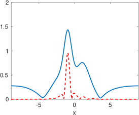
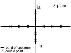
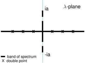
A                                                  B                                                  C

Figure 1: (A) Sample time slice showing the amplitude of $u$ (solid line) versus magnitude of $\beta u\left[{\cal H}\left(|u|^{2}\right)\right]_{x}$ (dash line). The Floquet spectrum of: (B) the Stokes wave with $\displaystyle\lfloor{aL}/{\pi}\rfloor=2$ and (C) the even three phase solution (13). Due to the Schwarz symmetry of the Z-S problem, we subsequently only display the spectrum in the upper half $\lambda$-plane.

2.2 Spatially periodic breather solutions of the NLS equation

Explicit expressions for the spatially periodic breathers (SPBs) can be derived using the Bäcklund-gauge transformation (BT) for the NLS equation [23]. For an unstable Stokes wave with $N$ UMs, a single BT at the complex double point $\lambda^{d}_{j}$, $1\leq j\leq N$, generates the single mode SPB, $U^{(j)}(x,t)$ corresponding to the j-th UM [4]:

$$U^{(j)}(x,t)=a\,e^{2\mathrm{i}a^{2}t}\,\left(\frac{1+2\,\mathrm{e}^{\sigma_{j}t+2\mathrm{i}\phi_{j}+\gamma}\cos\mu_{j}x+A\,\mathrm{e}^{2(\sigma_{j}t+2\mathrm{i}\phi_{j}+\gamma)}}{1+2\,\mathrm{e}^{\sigma_{j}t+\gamma}\cos\mu_{j}x+A\,\mathrm{e}^{2(\sigma_{j}t+\gamma)}}\right)$$ (8)

where $\mu_{j}=2\pi j/L$, $\sigma_{j}=2i\mu_{j}\lambda_{j}$, $\sin\phi_{j}=\mu_{j}/2a$, $A=\sec^{2}\phi_{j}$, and $\gamma$ is an arbitrary phase. $U^{(j)}(x,t)$ is localized in time: as $t\rightarrow\pm\infty$ the SPB exponentially approaches a phase shift of the Stokes wave at the rate $\sigma_{j}$. Figures 2A-B show the amplitudes of the two distinct single mode SPBs, $U^{(1)}(x,t)$ and $U^{(2)}(x,t)$.

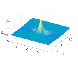
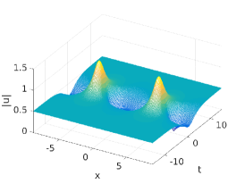
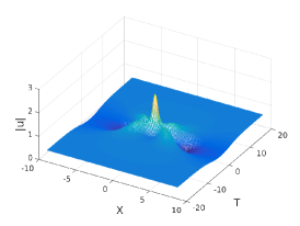
A                                                  B                                                  C

Figure 2: SPBs over a Stokes wave with $N=2$ UMs, $a=.5$, $L=4\sqrt{2}\pi$: Amplitudes of (A-B) single mode SPBs $|U^{(1)}(x,t,\rho)|$ and $|U^{(2)}(x,t,\rho)|$ ($\rho=\beta=0$) and (C) two-mode SPB $|U^{(1,2)}(\rho,\tau)|$ ($\rho=\tau=0$).

When the Stokes wave has $N\geq 2$ UMs, the BT can be iterated to obtain multi-mode SPBs. The family of two-mode SPB with wavenumbers $\mu_{i}$ and $\mu_{j}$ is obtained by applying the BT successively at complex $\lambda_{i}^{d}$ and $\lambda_{j}^{d}$ and is given by :

$$U^{(i,j)}(x,t;\rho,\tau)=a\mathrm{e}^{2\mathrm{i}a^{2}t}\frac{N(x,t;\rho,\tau)}{D(x,t;\rho,\tau)}.$$ (9)

The exact formula is provided in [31]. The parameters $\rho$ and $\tau$ determine the time at which the first and second modes become excited, respectively. Figure 2C shows the amplitude of the “coalesced” two mode SPB $U^{(1,2)}(x,t;0,0)$ where the two modes are excited simultaneously.

Note: The BT is isospectral: $\sigma(u_{a}(t))=\sigma(U^{(j)}(x,t))=\sigma(U^{(i,j)}(x,t))$. The Stokes wave with $N=2$ UMs and each of the SPBs shown in Figures 2A-C share the same Floquet spectrum (given in Figure 1B).

2.3 Perturbation analysis: Spectrum for damped SPB data

We are interested in the fate of the complex double points under the NLD-HONLS perturbation as they characterize the SPB initially. The linearized initial conditions for the one and two mode SPBs are obtained by choosing $t$ and $\gamma$ in formulas (8) and (9) such that $\epsilon_{s}=4\mathrm{i}\sin\phi_{s}\,\mathrm{e}^{\sigma_{s}t+\gamma}$, $s=i,j$, are small. Neglecting second order terms we obtain the linearized initial conditions

$$U^{(j)}(x,0) = a\,\left(1+\epsilon_{j}\,\mathrm{e}^{\mathrm{i}\phi_{j}}\cos\mu_{j}x\right),$$

$$U^{(i,j)}(x,0) = a\,\left(1+\epsilon_{i}\,\mathrm{e}^{\mathrm{i}\phi_{i}}\cos\mu_{i}x+\epsilon_{j}\,\mathrm{e}^{\mathrm{i}\phi_{j}}\cos\mu_{j}x\right),$$

where $\phi_{s}=\pi/4$, $s=i,j$. For small time $h$, we obtain the following first order approximation

$$U_{\epsilon,\beta}^{(j)}(x,h) = a\left[1+\tilde{\epsilon}_{j}\left(\mathrm{e}^{\mathrm{i}\tilde{\phi}_{j}}\cos\mu_{j}x+r_{j}\,\mathrm{e}^{\mathrm{i}\tilde{\theta}_{j}}\sin\mu_{j}x\right)\right]=a\left[1+\tilde{\epsilon}_{j}f_{j}\right],\qquad\tilde{\phi}_{s}\neq\tilde{\theta}_{s}$$

$$U_{\epsilon,\beta}^{(i,j)}(x,h) = a\left[1+\tilde{\epsilon}_{i}f_{i}+\tilde{\epsilon}_{j}f_{j}\right]$$

where $\tilde{\phi}_{s},\tilde{\theta}_{s},\tilde{\epsilon}_{s},r_{s}$ are functions of $h$ and the NLD-HONLS parameters $\epsilon$ and $\beta$, for $s=i,j$. Letting $\epsilon=\tilde{\epsilon}_{s}$ and suppressing their explicit dependence on $\epsilon,\beta,h$ the data is of the general form

$$u=a+\epsilon\left[f_{i}+Q\,f_{j}\right]=a+\epsilon u^{(1)}$$ (10)

where $r_{s}\neq 0$ and $Q$ can be 0 or 1, depending on whether a one or two mode SPB is under consideration.

In [21], via perturbation anlysis we examined the splitting of complex double points for data of the generic form (10). Briefly, at the double points $\lambda_{n}$ we assume the perturbation expansions

$$\lambda_{n}=\lambda_{n}^{(0)}+\epsilon\lambda_{n}^{(1)}+\epsilon^{2}\lambda_{n}^{(2)}+\cdots,\qquad\mathbf{v}_{n}=\mathbf{v}_{n}^{(0)}+\epsilon\mathbf{v}_{n}^{(1)}+\epsilon^{2}\mathbf{v}_{n}^{(2)}+\cdots$$

Substituting these expansions into Equation (2) the following ${\cal O}(\epsilon)$ correction to $\lambda_{n}$ is obtained :

$$\left(\lambda_{n}^{(1)}\right)^{2}=\left\{\begin{array}[]{ll}\frac{a^{2}}{4\lambda_{n}^{2}}\left[\sin(\omega_{n}+\tilde{\phi}_{n})\sin(\omega_{n}-\tilde{\phi}_{n})\right.&\\ \qquad+r_{n}^{2}\sin(\omega_{n}+\tilde{\theta}_{n})\sin(\omega_{n}-\tilde{\theta}_{n})&\quad n=i,j\\ \left.\qquad+\mathrm{i}r_{n}\sin(\tilde{\theta}_{n}-\tilde{\phi}_{n})\sin 2\omega_{n}\right]\\ 0&\quad n\neq i,j\end{array}\right.$$ (11)

where $\tan\omega_{n}=Im\left(\lambda_{n}^{(0)}\right)/k_{n}$ and $\tilde{\phi}_{j}\neq\tilde{\theta}_{j}\pm n\pi$. At $\mathcal{O}(\epsilon)$ there is a correction only to the double points $\lambda_{n}$, $n=i,j$. An examination of $\Delta$ in a neighborhood of $u^{(0)}$ finds the band of continuous spectrum along the imaginary axis splits asymmetrically at $\lambda_{n}^{(0)}$ into two disjoint bands in the upper half plane. As an example, see Figure 3C. The other double points do not experience an $\mathcal{O}(\epsilon)$ correction [21].

The ${\cal O}(\epsilon^{2})$ correction is of the form

$$\left(\lambda_{n}^{(2)}-\beta_{n}\right)^{2}=\left\{\begin{array}[]{ll}\alpha_{n}^{+}\alpha_{n}^{-}&\quad n=2i,2j,i+j,j-i\\ 0&\quad\mbox{for all other cases}\end{array}\right.$$ (12)

Only the double points $\lambda_{n}^{(0)}$ with $n=2i,2j,i+j$, or $j-i$ split at $\mathcal{O}(\epsilon^{2})$. All other double points experience an $\mathcal{O}(\epsilon^{2})$ translation. This calculation can be carried to higher order $\mathcal{O}(\epsilon^{m})$. In the simple example of a damped single mode SPB, $U_{\epsilon,\gamma}^{(j)}(x,t)$, only the double points $\lambda_{n}^{(0)}$ which correspond to a resonant mode $n=mj$ will split at order $\mathcal{O}(\epsilon^{m})$ whereas the splitting is zero for $\lambda_{n}^{(0)}$, $n\neq mj$ [21].

2.4 Soliton-like structures

Under the NLD-HONLS flow, the complex double points present initially in the spectrum of an SPB may split, creating additional complex bands of spectrum. As time evolves one or two of the bands may shrink significantly and their lengths become tiny (see e.g. Figure 4F, Figure 7C). For a qualitative understanding of the waveforms, we view the emergence of the tiny bands of spectrum as corresponding to nonlinear modes which have developed a one or two “soliton-like structure”.

Insight into the limiting behavior of solutions as gaps in the spectrum open and close is obtained by considering the family of 3-phase solutions of the NLS equation [4]:

$$u_{0}(x,t)=\frac{\kappa}{\sqrt{2}}\mathrm{e}^{\mathrm{i}t}\frac{\mbox{cn}\left(\sqrt{\frac{1+\kappa}{2}}x,k\right)\,\mbox{cn}(t,\kappa)+\mathrm{i}\sqrt{1+\kappa}\,\mbox{dn}\left(\sqrt{\frac{1+\kappa}{2}}x,k\right)\,\mbox{sn}(t,\kappa)}{\sqrt{1+\kappa}\,\mbox{dn}\left(\sqrt{\frac{1+\kappa}{2}}x,k\right)-\mbox{cn}\left(\sqrt{\frac{1+\kappa}{2}}x,k\right)\,\mbox{dn}(t,\kappa)},$$ (13)

where $0<\kappa<1$, and $k=\sqrt{\frac{1-\kappa}{1+\kappa}}$. The solutions are periodic in space and quasi-periodic in time; the spatial period, $L_{x}$, and the temporal period of the modulated phase, $L_{t}$, are functions of the complete elliptic integrals of the first kind, ${{\cal K}_{x}(k)}$ and ${{\cal K}_{t}(\kappa)}$ respectively.

The Floquet spectrum of $u_{0}(t)$ has two gaps in the spectrum along the imaginary axis as shown in Figure 1C. As $\kappa\rightarrow 1$ in (13), the gaps close to complex double points, and $u_{0}(x,t)$ limits to a scaling of the SPB given in Equation (8). On the other hand as $\kappa\rightarrow 0$, $u_{0}(x,t)$ limits to a scaling of the NLS soliton solution (given in Equation (14)) and the bands shrink to discrete points.

2.4.1 Soliton solutions

Complete information about the one and two soliton solutions, obtained using the inverse scattering theory, is contained in the scattering data [24]. The discrete spectra in the upper half plane, $\lambda_{n}$, are the zeros of the first Jost coefficient. Given $\lambda_{n}$, the soliton solutions are as follows:

One-soliton: Consider the discrete eigenvalue $\lambda=\xi+\mathrm{i}\eta$. Then the associated one-soliton solution is given by

$$u(x,t)=2\mathrm{i}\eta\,\mbox{sech}\left\{2\eta\left[x-x_{0}+4\xi t\right]\right\}\mathrm{e}^{\mathrm{i}\left[2\xi x+4\left(\xi^{2}-\eta^{2}\right)t+\phi\right]}$$ (14)

where $\xi,\eta,x_{0},\phi$ are constants physically representing the velocity ($4\xi$), the width and height ($\eta$), the initial center ($x_{0}$), and the phase ($\phi$) of the envelope, respectively.

Two-soliton: Consider the discrete eigenvalues $\lambda_{n}=\xi_{n}+\mathrm{i}\eta_{n}$, $n=1,2$. Define the quantities

$$\begin{array}[]{ll}\phi_{n}&=\pi/2-\arctan\left[\frac{(\xi_{n}-\xi_{\tilde{n}})^{2}+\eta_{n}^{2}-\eta_{\tilde{n}}^{2}}{2\eta_{\tilde{n}}(\xi_{n}-\xi_{\tilde{n}})}\right],\quad\tilde{n}=3-n,\\ \theta_{n}(t)&=\theta_{n}^{0}-4\xi_{n}\eta_{n}t,\qquad\sigma_{n}(t)=\sigma_{n}^{0}+2\left(\xi_{n}^{2}-\eta_{n}^{2}\right)t,\\ \Delta(x,t)&=\cosh\left[2(\eta_{1}+\eta_{2})x-\theta_{1}(t)-\theta_{2}(t)\right]\\ &+\frac{4\eta_{1}\eta_{2}}{(\xi_{1}-\xi_{2})^{2}+(\eta_{1}-\eta_{2})^{2}}\cos\left[2(\xi_{1}-\xi_{2})x+\sigma_{1}(t)-\sigma_{2}(t)\right]\\ &+\frac{(\xi_{1}-\xi_{2})^{2}+(\eta_{1}+\eta_{2})^{2}}{(\xi_{1}-\xi_{2})^{2}+(\eta_{1}-\eta_{2})^{2}}\cosh\left[2(\eta_{1}-\eta_{2})x-\left(\theta_{1}(t)-\theta_{2}(t)\right)\right]\end{array}$$

where $\theta_{n}(t)$ and $\sigma_{n}(t)$ give the position and phase of the solitons. Then the associated two-soliton solution, with velocities given in terms of $\xi_{n}$ , is given by [25]

$$\begin{array}[]{ll}u(x,t)=&-\frac{2}{\Delta}\left(\frac{(\xi_{1}-\xi_{2})^{2}+(\eta_{1}+\eta_{2})^{2}}{(\xi_{1}-\xi_{2})^{2}+(\eta_{1}-\eta_{2})^{2}}\right)^{1/2}\\ &\times\left[2\eta_{1}\cosh\left(2\eta_{2}x-\theta_{2}(t)-\mbox{i}\phi_{1}\right)\mbox{e}^{-2\mbox{i}\xi_{1}x-\mbox{i}\sigma_{1}(t)}+2\eta_{2}\cosh\left(2\eta_{1}x-\theta_{1}(t)-\mbox{i}\phi_{2}\right)\mbox{e}^{-2\mbox{i}\xi_{2}x-\mbox{i}\sigma_{2}(t)}\right].\end{array}$$ (15)

3 Numerical Investigations

In this section we investigate the effects of nonlinear dissipation and higher order nonlinearities on the routes to stability of the single and multi-mode SPBs. We appeal to the Floquet spectral theory of the NLS equation to interpret and provide a characterization of the perturbed dynamics in terms of nearby solutions of the NLS equation.

The NLD-HONLS equation is solved numerically using a very accurate exponential integrator (ETD4RK). The ETD4RK integrator combines a Fourier mode decomposition in space with a fourth order exponential Runge-Kutta method in time which uses Pade approximations of the matrix exponential terms [28, 29] (see the Appendix for the ETD4RK scheme and its convergence properties). The number of Fourier modes and the time step used depends on the complexity of the solution. For example, for initial data in the two UM regime, $L=4\sqrt{2}\pi$, $N=256$ Fourier modes are used with time step $\Delta t=10^{-3}$. As a benchmark, with this resolution the invariants of the HONLS equation, (the mass $E(t)=\int_{0}^{L}|u(x,t)|^{2}\,dx$, momentum $P(t)=i\int_{0}^{L}\left(u(x,t)^{*}u_{x}(x,t)-u(x,t)u_{x}(x,t)^{*}\right)dx$, and Hamiltonian

$$H(t)=\int_{0}^{L}\left\{|u_{x}|^{2}-|u|^{4}-\mathrm{i}\epsilon\left[1/4\left(u_{x}u_{xx}^{*}-u_{x}^{*}u_{xx}\right)+2|u|^{2}\left(u^{*}u_{x}-uu_{x}^{*}\right)-|u|^{2}\left[\mathcal{H}\left(|u|^{2}\right)\right]_{x}\right]\right\}\,dx$$ (16)

are preserved with an $\mathcal{O}(10^{-11})$ accuracy for $0\leq t\leq 100$. Furthermore, in our earlier studies of the NLS equation, the ETD4RK scheme was shown to accurately preserve the Floquet spectrum [30]. This is an important feature in our studies as the Floquet spectrum is a significant tool in the analysis of rogue waves.

Setup of the experiments: The initial data used in the numerical experiments is generated using exact SPB solutions of the integrable NLS equation. The perturbed SPBs are indicated with subscripts: $U^{(j)}_{\epsilon,\beta}(x,t)$ is the solution of the NLD-HONLS Equation (1) for one-mode SPB initial data $U^{(j)}(x,T_{0})$. Likewise $U^{(i,j)}_{\epsilon,\beta}(x,t)$ is the solution to (1) for two-mode SPB initial data. The “$N$ UM regime” refers to the range in the amplitude $a$ and period $L$ for which the underlying Stokes wave initially has $N$ unstable modes.

In the current study we systematically vary $T_{0}\in[-5,0]$ to allow the NLD-HONLS solutions to be initialized with SPB data at different stages of their development, i.e. from the early stage of the MI when there is strong growth ($T_{0}=-5$) through the nonlinear stage when the MI is saturating ($T_{0}=0$). For each damped SPB under consideration the complete set of diagnostics is presented for one value of $T_{0}$. Qualitative differences in the the solution as $T_{0}$ is varied are either discussed or summarized graphically. The perturbation parameters are set at $\epsilon=0.05$ and $\beta=0.2$. For $U^{(1,2)}_{\epsilon,\beta}(x,t)$, which displays more complex behavior, $\beta$ is also varied $0.01\leq\beta\leq 0.2$.

Nonlinear mode decomposition of the NLD-HONLS flow: The Floquet spectral decomposition of the NLD-HONLS data is computed at each time $t$, $0\leq t\leq 100$, using the numerical procedure developed by Overman et. al. [26]. After solving system (2), the discriminant $\Delta$ is constructed. The zeros of $\Delta\pm 2$ are determined using a root solver based on Müller’s method and then the curves of spectrum are filled in. The spectrum is calculated with an accuracy of ${\mathcal{O}}(10^{-6})$.

Notation used in the spectral plots: The periodic/antiperiodic spectrum is indicated with a large “$\times$” when $\Delta=-2$ and with a large box when $\Delta=2$. The continuous spectrum is indicated with small “$\times$” when $\Delta$ is negative and with small boxes when $\Delta$ is positive. Since the NLS spectrum is symmetric under complex conjugation, the spectrum is displayed only in the upper half $\lambda$-plane.

“Soliton-like” Criterion: The lengths of the bands of spectrum in the upper half plane associated with the dominant modes are monitored. When these bands are tiny we view the corresponding modes of the $N$-phase solution as having a soliton-like structure. Let the length of a band with endpoints $\lambda_{m}$ and $\lambda_{n}$ be given by $\gamma(t;\lambda_{m},\lambda_{n})$. If one or two of the band lengths satisfy

$$\gamma(t;\lambda_{m},\lambda_{n})=|\lambda_{m}(t)-\lambda_{n}(t)|<0.025,$$ (17)

then the spectrum is said to be in a one or two soliton-like configuration.

Rogue Wave Criterion: To determine the occurence of rogue waves we monitor the strength function

$$S(t):=\frac{\max\limits_{x}|u(x,t)|}{H_{s}(t)},$$

where $H_{s}(t)$ is the significant wave amplitude, defined as four times the standard deviation of the surface amplitude. A rogue wave is said to occur at $t^{*}$ if $S(t^{*})>2.2$. In the strength plots the horizontal line indicates the reference strength for a rogue wave.

Saturation time of the instabilities: The spectral analysis is complemented by an examination of the saturation time of the instabilities for the nonlinear damped SPBs. This is accomplished by examining the growth of small perturbations in the initial data of the following form,

$$U^{(j)}_{\epsilon,\beta,\delta}(x,0)=U^{(j)}(x,0)+\delta f_{k}(x),\qquad\mbox{and}\qquad U^{(i,j)}_{\epsilon,\beta,\delta}(x,0)=U^{(i,j)}(x,0)+\delta f_{k}(x)$$ (18)

where $f_{k}(x)=\cos\mu_{k}x+r_{k}e^{i\phi_{k}}\sin\mu_{k}x$, $\mu_{k}=2\pi k/L$, $1\leq k\leq 2$.

To determine whether $U^{(j)}_{\epsilon,\beta}(x,t)$ and $U^{(j)}_{\epsilon,\beta,\delta}(x,t)$ remain close as time evolves we monitor the evolution of $d(t)$,

$$d(t)=\|u_{\delta}(x,t)-u(x,t)\|_{H^{1}}$$ (19)

where $\|f\|^{2}_{H^{1}}=\int_{-L/2}^{L/2}\left(|f_{x}|^{2}+|f|^{2}\right)\,dx.$ We consider the solution to have stabilized under the NLD-HONLS flow once $d(t)$ saturates.

From the Floquet perspective, we find the NLD-HONLS solutions are stabilized by nonlinear damping once complex double points and complex critical points are eliminated in the spectral decomposition of the data.

3.1 The NLD-HONLS SPB in the one UM regime: $a=0.5,L=2\sqrt{2}\pi$

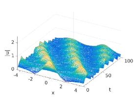
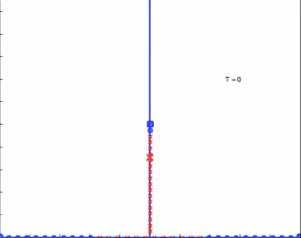
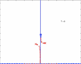
A                                                  B                                                  C

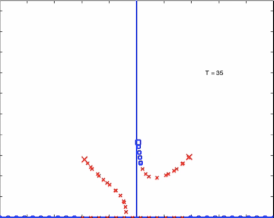
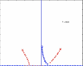
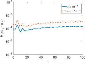
D                                                  E                                                  F

Figure 3: One UM regime: (A) $|U^{(1)}_{\epsilon,\beta}(x,t)|,T_{0}=0$, for $0\leq t\leq 100$. Spectrum at (B) $t=0$, (C) $t=3$, (D) $t=35$, (E) $t=59.9$, and (F) $d(t)$ for $f_{1}(x)$, $\delta=10^{-4},5\times 10^{-4}$.

The NLD-HONLS parameters are $\epsilon=0.05$ and $\beta=0.2$. Figure 3A shows the surface $|U^{(1)}_{\epsilon,\beta}(x,t)|$ for initial data generated using Equation (8) with $T_{0}=0$ for $0<t<100$. This choice of $T_{0}$ initializes the solution near the peak of the SPB $U^{(1)}(x,t)$.

The Floquet spectrum evolves as follows: At $t=0$, the spectrum in the upper half plane consists of a single band of spectrum with end point at $\lambda_{0}^{s}=0.5\mathrm{i}$, indicated by a large “box”, and one imaginary double point at $\lambda_{1}^{d}=0.3535\mathrm{i}$, indicated by a large “$\times$” (Figure 3B). Under the NLD-HONLS flow $\lambda_{1}^{d}$ immediately splits asymmetrically into $\lambda_{1}^{\pm}$, with the upper band of spectrum in the right quadrant and the lower band in the left quadrant (referred to as a right state since the waveform is characterized by a single damped modulated mode traveling to the right). The right state is clearly visible at $t=3$ in Figure 3C. The numerically observed evolution of spectrum for $U_{\epsilon,\beta}^{(1)}(x,t)$ for short time is confirmed by the perturbation analysis. Equation (11) indicates the complex double point $\lambda_{1}^{d}$, at which the initial SPB was constructed, splits asymmetrically at $\mathcal{O}(\epsilon)$.

As time evolves the spectrum persists in a right state (Figure 3D) with the upper band increasing in length, although oscillating in length as it does so. In Figure 3E the vertex of the loop eventually touches the origin at $t\approx 59.9$. Subsequently the spectrum has three bands emanating off the real axis, with endpoints $\lambda_{1}^{-},\lambda_{0}^{s},\lambda_{1}^{+}$ which, as damping continues, decrease in length. Complex double points/critical points do not appear in the spectral evolution for $t>0$, indicating stability.

Figure 3F shows the evolution of $d(t)$ for $U_{\epsilon,\beta}^{(1)}(x,t)$ using $f_{1}$ and $\delta=10^{-4},5\times 10^{-4}$ (see Equation (18)). There is no significant growth in $d(t)$ and $U_{\epsilon,\beta}^{(1)}(x,t)$ is stable for $t>0$. The evolution of $d(t)$ is consistent with the prediction of stability from the evolution of the spectrum. We do not show a strength plot for $U_{\epsilon,\beta}^{(1)}(x,t)$ as rogue waves do not occur in its evolution.

As $T_{0}$ is varied in the initial data, the spectral evolution obtained for $U_{\epsilon,\beta}^{(1)}(x,t)$ is qualitatively similar (a right state is consistently obtained) to the spectrum shown in Figure 3. Complex critical points or double points do not occur in the spectral evolution for $t>0$. As a result, $U_{\epsilon,\beta}^{(1)}(x,t)$ in the one UM regime evolves as a stable damped traveling breather, exhibiting regular behavior, and can be characterized as a continuous deformation of a noneven 3-phase solution. The amplitude of the oscillations of $U_{\epsilon,\beta}^{(1)}(x,t)$ decreases and the frequency increases until small fast oscillations about the damped Stokes wave, visible in Figure 3A, appear.

In the one UM regime the main differences in the NLD-HONLS evolution, as compared with linear damped HONLS in [27], are i) the lack of complex critical points in the spectral evolution and ii) the small fast time scale oscillations in the band lengths which correspond to small higher order oscillations in the temporal frequency.

3.2 NLD-HONLS SPBs in the two UM regime: $a=0.5,L=4\sqrt{2}\pi$

We examine the evolution of the two distinct perturbed single mode SPBs, $U_{\epsilon,\beta}^{(1)}(x,t)$ and $U_{\epsilon,\beta}^{(2)}(x,t)$, and the perturbed two mode SPB $U_{\epsilon,\beta}^{(1,2)}(x,t)$. Recall that $\sigma(u_{a}(t))=\sigma(U^{(j)}(x,t))=\sigma(U^{(i,j)}(x,t))$. As a result, the Floquet spectrum at $t=0$ is identical for all the numerical experiments in the two UM regime. The NLD-HONLS parameters are $\epsilon=0.05$ and $\beta=0.2$.

3.2.1 Characterization of $U_{\epsilon,\beta}^{(1)}(x,t)$:

Figure 4A shows the surface $|U_{\epsilon,\beta}^{(1)}(x,t)|$ for $0<t<100$ for initial data generated using Equation (8) for $T_{0}=-5$. The Floquet spectrum at $t=0$ is given in Figure 4B. The end point of the band of spectrum at $\lambda_{0}^{s}=0.5\mathrm{i}$ is indicated by a “box”. There are two complex double points at $\lambda_{1}^{d}=0.4677\mathrm{i}$ and $\lambda_{2}^{d}=0.3535\mathrm{i}$, indicated by an “$\times$” and a “box”, respectively. Both complex double points split asymmetrically yielding three bands in the upper half complex plane as seen in Figure 4C at $t=3.5$. The numerically observed evolution of spectrum for $U_{\epsilon,\beta}^{(1)}(x,t)$ for short time is confirmed by the perturbation analysis. Equations (11) - (12) indicate both complex double points split asymmetrically: $\lambda_{1}^{d}$ at which the NLS SPB was constructed splits at ${\cal O}(\epsilon)$ into $\lambda^{\pm}_{1}$ while $\lambda_{2}^{d}$ splits at $\mathcal{O}(\epsilon^{2})$ into $\lambda_{2}^{\pm}$.

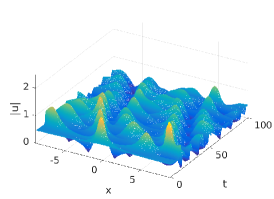
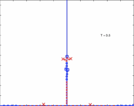
A                                                  B                                                  C

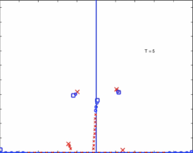
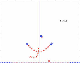
D                                                  E                                                  F

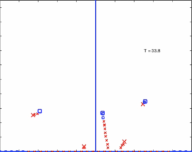
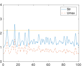
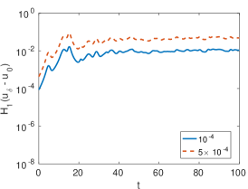
G                                                  H                                                  I

Figure 4: Two UM regime: (A) $|U^{(1)}_{\epsilon,\beta}(x,t)|,T_{0}=-5$, for $0\leq t\leq 100$, spectrum at (B) $t=0$, (C) $t=3.5$, (D) $t=5$, (E) $t=14.3$, (F) $t=15.2$, (G) $t=33.8$, (H) strength, and (I) $d(t)$ for $f_{2}(x)$, $\delta=10^{-4},5\times 10^{-4}$. Rogues between: 4.6 - 5.2, 14.6 - 15.5, 33.5 - 34.1. Stability peaks at: 15.2.

Subsequently the two upper bands with end points ($\lambda_{0}^{s},\lambda_{1}^{+}$) and ($\lambda_{1}^{-},\lambda_{2}^{+}$) decrease in length while they detach and move away from the imaginary axis, yielding a five-phase solution with one tiny band ($\lambda_{0}^{s},\lambda_{1}^{+}$) in the first quadrant and a somewhat larger band ($\lambda_{1}^{-},\lambda_{2}^{+}$) in the second quadrant and one band close to the imaginary axis ($\lambda_{2}^{-},\lambda_{R}$) where $\lambda_{R}$ is real, as seen at $t\approx 5$ in Figure 4D (note: we neglect the small bands emanating off the real axis related to the higher modes). Applying criteria (17), we find a soliton-like mode has emerged and the solution is “close” to a one soliton-like state.

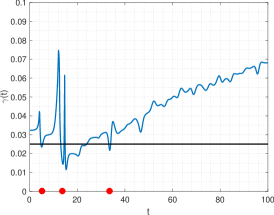
Figure 5: Variation of the length of the band $|\lambda_{0}^{s}-\lambda_{1}^{+}|$ of spectrum as a function of time. The horizontal line represents the upper bound for a one soliton-like state. The red dots represent the time a rogue wave occurs.

This soliton-like state satisfies the criterion of a rogue wave. The rogue wave is visible in the strength plot, Figure 4H, at $t\approx 5$. The spectrum remains near this state until $t\approx 5.5$. The lengths of the bands then increase and a sequence of bifurcations occur in rapid succession for $11<t<14.3$ with complex critical points forming, indicating instability of the corresponding nonlinear modes. The last complex critical point at $t=14.3$ is shown in Figure 4E. Subsequently the bands split and their lengths decrease until the band in the first quadrant again satisfies the one soliton-like criteria at $t=15.2$ in Figure 4F. A more pronounced rogue wave is observed in the strength plot at this time. The fluctuation in the band lengths occur once more, producing at $t=33.8$ the last soliton-like spectrum (Figure 4G) and the last rogue wave (Figure 4H). The spectral band lengths then increase and settle into a typical $5$-phase state with no further rogue wave activity.

The variation in the band length $\gamma(t)=|\lambda_{0}^{s}-\lambda_{1}^{+}|$ for the band in the upper right quadrant are shown in Figure 5. The variation in the band length for the band in the upper left quadrant is not shown as it never satisfies the criteria for a soliton-like state. Recalling equation (17), a one soliton-like state occurs at $t^{*}$ if $\gamma(t^{*})<0.025$. In Figure 5 the horizontal line indicates the upper bound on the band length for a soliton-like state. Additionally a red dot on the $t$-axis indicates the time at which a rogue wave occurs providing a correlation between one soliton-like states and rogue waves.

Observation: Soliton-like rogue waves emerge in the NLD-HONLS flow. Each time a rogue wave is observed in the strength plot of $U^{(1)}_{\epsilon,\beta}(x,t)$ (i.e. $S(t)>2.2$ at $t=5$, $t=15.2$, and $t=33.8$), the corresponding spectrum is in a one soliton-like configuration.

We remark that the emergence of the one soliton-like structure in the evolution of the nonlinear damped $U_{\epsilon,\beta}^{(1)}(x,t)$ in the two UM regime was not observed in the linear damped HONLS study [21].

The evolution of $d(t)$ for $U_{\epsilon,\beta}^{(1)}(x,t)$ is given in Figure 4H with $f_{2}$ for $\delta=10^{-4},5\times 10^{-4}$ (see Equation (18)). The perturbation $f_{2}$ is chosen in the direction of the unstable mode associated with $\lambda_{2}^{d}$. The growth in $d(t)$ saturates by $t=15.2$, in agreement with the stabilization time determined by the last critical point in the nonlinear spectral decomposition of the solution at $t=14.3$.

For $U_{\epsilon,\beta}^{(1)}(x,t)$ in the two-UM regime, both $\lambda_{1}^{d}$ and $\lambda_{2}^{d}$ resonate with the perturbation. The route to stability, for $T_{0}\in[-5,-1]$ is characterized by the appearance of a one soliton-like structure which corresponds to rogue wave events. As $T_{0}\rightarrow 0$, more complex critical points appear in the spectral decomposition and it takes longer for the damped solution to stabilize. Fewer rogue waves may occur, and these weaker rogue waves are no longer associated with a one soliton-like structure.

3.2.2 Characterization of $U^{(2)}_{\epsilon,\beta}(x,t)$:

We now consider $U^{(2)}_{\epsilon,\beta}(x,t)$ with initial data generated using Equation (8) with $T_{0}=-5$. $U^{(1)}(x,t)$ and $U^{(2)}(x,t)$ are both single mode SPBs over the same Stokes wave. Even so, their respective evolutions under the NLD-HONLS flow are quite different. Notice in Figure 6A the surface of $|U_{\epsilon,\beta}^{(2)}(x,t)|$ for $0\leq t\leq 100$ is a damped traveling breather, exhibiting regular behavior, in contrast to the irregular behavior of $|U_{\epsilon,\beta}^{(1)}(x,t)|$ in the two UM regime. Further, as shown in the strength plot Figure 6F, rogue wave events do not occur in the evolution of $U^{(2)}_{\epsilon,\beta}$.

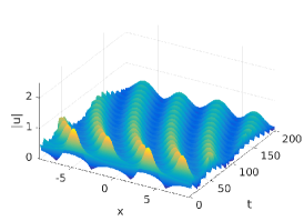
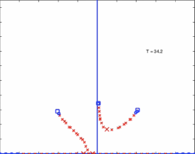
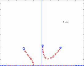
A                                                  B                                                  C

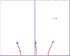
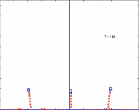
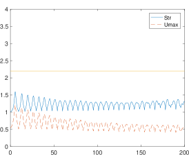
D                                                  E                                                  F

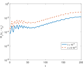
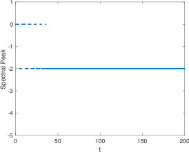
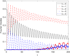
G                                                  H                                                  I

Figure 6: Two UM regime: (A) $|U^{(2)}_{\epsilon,\beta}(x,t)|,T_{0}=-5$, for $0\leq t\leq 100$, spectrum at (B) $t=34.2$, (C) $t=44$, (D) $t=75$, (E) $t=188$, (F) strength, (G) $d(t)$ for $f_{1}(x)$, $\delta=10^{-4},5\times 10^{-4}$, (H) spectral peak, (I) Fourier modes.

The spectrum of the initial data $U_{\epsilon,\beta}^{(2)}(x,0)$ is given in Figure 4B and has two complex double points. Under the NLD-HONLS flow $\lambda_{2}^{d}$ immediately splits asymmetrically into $\lambda_{2}^{\pm}$, forming a right traveling breather with the upper band in the right quadrant and the lower band in the left quadrant. Significantly, the first double point $\lambda_{1}^{d}$ does not split. Figure 6B clearly shows that $\lambda_{1}^{d}$, indicated by the large “$\times$”on the upper band, has not split at $t=34.2$.

The short time perturbation results, Equations (11) - (12) show that only the double point $\lambda_{2}^{d}$ associated with the SPB initial data $U^{(2)}(x,0)$ splits at ${\cal O}(\epsilon)$ under the NLD-HONLS. The double points $\lambda_{2m}^{d}$ split at $\mathcal{O}(\epsilon^{m})$ while $\lambda_{l}^{d}$, $l\neq 2m$ do not split, confirming for short time the numerically observed evolution of spectrum for $U_{\epsilon,\beta}^{(2)}(x,t)$. In fact, $\lambda_{1}^{d}$, which corresponds to a non-resonant mode, is observed to translate along a band of spectrum but does not split for the duration of the NLD-HONLS evolution, $0\leq t\leq 200$, see Figures 6B-E.

A distinctive feature of the spectral evolution for $U_{\epsilon,\beta}^{(2)}(x,t)$ is that the solution gains an unstable mode corresponding to $\lambda_{3}^{d}$. At $t\approx 30$, enough energy has been transferred to the third mode (originally inactive) so that $\lambda_{3}^{d}$ starts to move from the real axis onto a band of spectrum in the upper half complex plane. The additional double point is clearly visible in Figure 6C at $t=44$. The vertex of the upper band of spectrum touches the real axis at $t=51.1$ and subsequently, as seen in Figure 6D at $t=75$, there are three bands of spectrum emanating from the real axis, two of which have complex double points

As time evolves $\lambda_{1}^{d}$ and $\lambda_{3}^{d}$ decrease in magnitude and at $t=188$ they become real double points, Figure 6E. This agrees with the stability plot, Figure 6G, which shows $d(t)$ grows due to the presence of instabilities until $t=188$. From the Floquet perspective $U_{\epsilon,\beta}^{(2)}(x,t)$ stabilizes slowly, evolving as a regular but unstable damped three-phase solution, until the complex double points become real at $t=188$.

An interesting aspect of the dynamics is that the growth of the instability associated with the complex double point $\lambda_{1}^{d}$ appears delayed. Figure 6G shows that the growth in $d(t)$ is more significant later in the experiment at $t\approx 60$. Since $\lambda_{1}^{d}$ does not split we would have expected to initially see significant growth in $d(t)$. A Fourier decomposition of the data shows that the waveform is undergoing frequency downshifting during the early stage of the experiment. Defining the dominant mode or spectral peak, $k_{peak}$, as the wave number $k$ for which $|\hat{u}_{k}|$ achieves its maximum, downshifting occurs when there is a shift down in $k_{peak}$ [15]. In Figure 6H we find downshifting becomes permanent about $t\approx 40$, with the energy flowing primarily from the zeroth Fourier mode to the 2nd Fourier mode.

Figure 6I is a plot of the Fourier modes for NLD-HONLS for the perturbed initial data
$U^{(2)}_{\epsilon,\beta,\delta}(x,0)=U^{(2)}(x,T_{0})+\delta f_{1}(x)$ (see Equation (18)), $0<t<200$. The dark red and blue curves correspond to the $k=1$ and $k=3$ mode respectively. The Fourier mode plot demonstrates that even when the first mode is excited initially, frequency downshifting due to nonlinear damping inhibits the growth of the first mode which is then expressed as a higher order effect. We find $d(t)$ grows, i.e. $U_{\epsilon,\beta}^{(2)}(x,t)$ and $U_{\epsilon,\beta,\delta}^{(2)}(x,t)$ grow apart until $t=188$. This confirms the stabilization time obtained from the nonlinear spectral analysis and supports the observation that $\lambda_{1}$ does not split.

For $U_{\epsilon,\beta}^{(2)}(x,t)$ in the two-UM regime, only $\lambda_{2}^{d}$ resonates with the perturbation. Since one of the unstable modes does not resonate with the perturbation, the dynamics is simplified and organized. $U_{\epsilon,\beta}^{(2)}(x,t)$ is a damped traveling breather exhibiting regular behavior and can be characterized as a continuous deformation of a noneven 3-phase solution. Rogue waves do not appear in the evolution of $U_{\epsilon,\beta}^{(2)}(x,t)$. This broad characterization does not change as $T_{0}$ is varied.

3.2.3 Characterization of $U^{(1,2)}_{\epsilon,\beta}(x,t)$:

The two-mode SPB of highest amplitude is obtained when the modes are excited simultaneously and coalesce, i.e. for $\rho=\tau=0$ in Equation (9) (see Figure 2C). The coalesced two-mode SPB has come to be viewed as a “fundamental” two-mode rogue wave as it is more robust in the presence of small random variations of initial data [8]. In this subsection we examine the evolution of $U_{\epsilon,\beta}^{(1,2)}(x,t)$ for the coalesced SPB initial data as $T_{0}$ and $\beta$ are varied.

Figure 7A shows the surface $|U_{\epsilon,\beta}^{(1,2)}(x,t)|$ for $0<t<100$ for the coalesced SPB initial data using $T_{0}=-3.5$. The Floquet spectrum of the initial data, given in Figure 4B, contains two complex double points $\lambda_{1}^{d}$ and $\lambda_{2}^{d}$ which, under the NLD-HONLS flow, immediately split asymmetrically into $\lambda^{\pm}_{1}$ and $\lambda_{2}^{\pm}$, respectively (Figure 7B). The numerically observed evolution of spectrum for $U^{(1,2)}_{\epsilon,\beta}(x,t)$ for short time is confirmed by the perturbation results given in Equation (11) which indicate that under the NLD-HONLS flow both complex double points split asymmetrically at ${\cal O}(\epsilon)$.

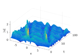
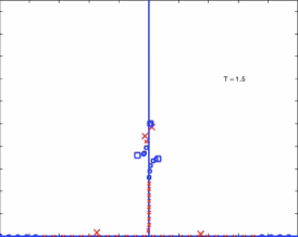
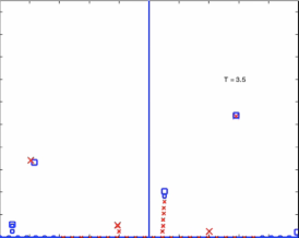
A                                                  B                                                  C

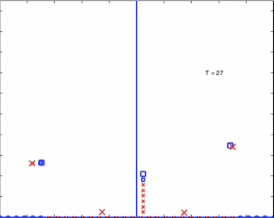
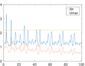
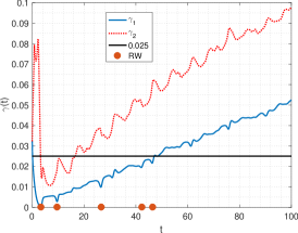
D                                                  E                                                  F

Figure 7: Two UM regime: (A) $|U^{(1,2)}_{\epsilon,\beta}(x,t)|,T_{0}=-3.5$, for $0\leq t\leq 100$, spectrum at (B) $t=1.5$, (C) $t=3.5$, (D) $t=27$, (E) strength, (F) Variation of the length of the band $|\lambda_{0}^{s}-\lambda_{1}^{+}|$ of spectrum as a function of time. The horizontal line represents the upper bound for a one soliton-like state. The red dots represent the time a rogue wave occurs.

Subsequently, the two upper bands of spectrum quickly pinch off from the imaginary axis and shrink significantly in length, entering a two soliton-like spectral configuration at $t=3.5$ (Figure 7C). The spectrum is in a two soliton-like state until $t\approx 18$ when one of the bands enlarges and the spectrum enters a one soliton state (e.g. see a sample one soliton-like spectrum at $t=27$ in Figure 7D). The spectral bands continue to enlarge as time evolves and the spectrum settles into a typical spectrum for a $5$-phase solution.

The variation in the band lengths $\gamma_{1}(t)=|\lambda_{0}^{s}-\lambda_{1}^{+}|$ and $\gamma_{2}(t)=|\lambda_{1}^{-}-\lambda_{2}^{+}|$ are shown in Figure 7F. The horizontal line in Figure 7F indicates the upper bound (given by equation (17)) on the band lengths for a one or two soliton-like state. Additionally a red dot on the $t$-axis indicates the time at which a rogue wave occurs providing a correlation between one or two soliton-like states and rogue waves.

In this experiment, which used initial data for the coalesced SPB closer to the Stokes wave, the spectrum is in a one or two soliton-like configuration whenever a rogue wave occurs. The first two rogue waves observed at $t\approx 3.5$ and $t\approx 10$ in the strength plot (Figure 7E) appear when the spectrum is in a two soliton-like configuration and are considerably larger in amplitude than the rogue waves at $t\approx 27,42,46$ which occur when the spectrum is in a one soliton-like configuration.

Complex critical points do not appear in the spectral evolution for $t>0$. In Figure 8A there is no significant growth in $d(t)$ and $U_{\epsilon,\beta}^{(1,2)}$ is stable for $t>0$. $U_{\epsilon,\beta}^{(1,2)}$ can be characterized by a continuous deformation of a stable NLS five-phase solution, keeping in mind that the modes determined by the very small bands of spectrum are limiting to a soliton-like structure.

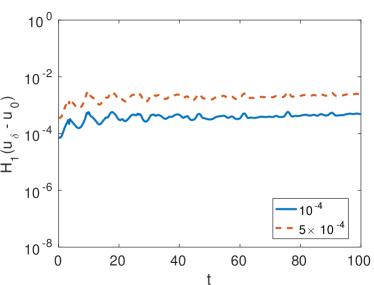
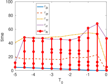
A                                                                   B

Figure 8: Two UM regime: (A) $d(t)$ for $f_{1}(x)$, $\delta=10^{-4},5\times 10^{-4}$. (B) The times $\tau_{2i}$, $\tau_{2f}$, $\tau_{1f}$, $\tau_{R}$, and $\tau_{rf}$, defined by (20), as $T_{0}$ varies.

Dependence of rogue wave activity on $T_{0}$: In the $U^{(1)}_{\epsilon,\beta}(x,t)$ example we found the spectrum transitioned repeatedly in and out of a one soliton-like state (see Figure 5). Transitioning repeatedly between one and two soliton-like states does not occur in $U^{(1,2)}_{\epsilon,\beta}(x,t)$. Instead, the evolution of the spectrum for $U^{(1,2)}_{\epsilon,\beta}(x,t)$ has the following pattern for all $T_{0}\neq 0$:

Both complex double points split $\rightarrow$ 2 soliton-like $\rightarrow$ 1 soliton-like $\rightarrow$ generic $N$-phase spectrum.

For $T_{0}\neq 0$ the time at which a two soliton-like spectrum is last observed is the time at which a one soliton-like spectrum is first observed. Thus, to examine the dependence of rogue wave activity on $T_{0}$ for $U^{(1,2)}_{\epsilon,\beta}(x,t)$, we determine the following:

$$\begin{array}[]{rcl}(a)\;\tau_{2i}&=&\mbox{the time at which a two soliton-like spectrum is first observed}\\ (b)\;\tau_{2f}&=&\mbox{the time at which a two-soliton-like spectrum is last observed}\\ (c)\;\tau_{1f}&=&\mbox{the time at which a one-soliton-like spectrum is last observed}\\ (d)\;\tau_{R}&=&\mbox{the times at which rogue waves occur}\\ (e)\;\tau_{rf}&=&\mbox{the time of the last rogue wave}\end{array}$$ (20)

Figure 8B provides the final times for : $\tau_{2f}$ a two soliton-like state, a one soliton-like state $\tau_{1f}$, the last rogue wave $\tau_{rf}$ for $U^{(1,2)}_{\epsilon,\beta}(x,t)$ for $T_{0}\in[-5,0)$. $T_{0}$ is incremented in steps of $0.5$. The red dots at each sampled $T_{0}$ provide a time-line for the rogue wave events. Correlating the $\tau$-times with the timeline for rogue waves we obtain the following

Observation: For the coalesced two mode SPB $U^{(1,2)}_{\epsilon,\beta}(x,t)$, all rogue waves emerge when the spectrum is in a one or two soliton-like configuration for all values of $T_{0}\in[-5,-1.5]$, i.e. for solutions initialized in the early to middle stage of the development of the MI.

Figure 9A provides the numerical solution $|U^{(1,2)}_{\epsilon,\beta}(x,5)|$ for $T_{0}=-5$ versus the two-soliton analytical solution (15) which uses the spectral data obtained from the spectral decomposition of the numerical solution. In formula (15) $\lambda_{1}$ and $\lambda_{2}$ are the midpoints of the two small bands that pinched off. Even though the NLD-HONLS soliton-like solution is over a non uniform finite background, near it’s peak it structurally appears in good agreement with the two soliton waveform.

There are other possible mechanisms for rogue wave development when the solutions are initialized as the MI is saturating. For $T_{0}\in[-1,0]$, the last rogue wave occurs after the spectrum has left a soliton-like state (for $T_{0}=0$ considerably later, see Figure 8B). Figure 9B shows the strength plot of $U_{\epsilon,\beta}^{(1,2)}(x,t)$ for initial data obtained using $T_{0}=0$, i.e. initializing at the peak of the SPB. A rogue wave occurs at $t=47$. Figure 9C clearly shows the spectrum at $t=47$ is not in a soliton-like configuration; the rogue wave occurs due to a superposition of the nonlinear modes.

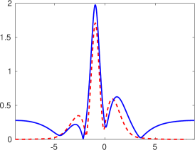
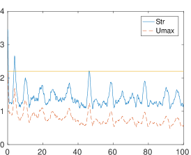
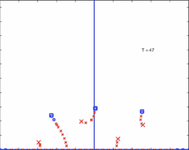
A                                                B                                                C

Figure 9: (A) $|U^{(1,2)}_{\epsilon,\beta}(x,5)|$ vs two-soliton analytical solution for $T_{0}=-5$. Two UM regime $|U^{(1,2)}_{\epsilon,\beta}(x,t)|,T_{0}=0$: (B) Strength for $0\leq t\leq 100$ and (C) spectrum at $t=47$.

4 Appendix

4.1 The Exponential Time Differencing Fourth-order Runge-Kutta scheme ETD4RK

A spectral spatial discretization of the NLS equation (when $\epsilon=0$ in Equation (1)) can be written as a system of ordinary differential equations of the form $\hat{u}_{t}+L\hat{u}=F(u)$, where $\hat{u}$ is the discrete Fourier transform of $u$, $L$ is a diagonal matrix, and $F$ is the discrete Fourier transform of the nonlinear term which is evaluated by transforming to physical space, evaluating the nonlinear terms, and transforming back to Fourier space. Using a fourth-order (2,2)-Pade approximation of $\mathrm{e}^{-z}$ the exponential time differencing fourth-order Runge-Kutta scheme ETD4RK is given by

$$\hat{u}_{h}^{n+1}=R_{2,2}(hL)\hat{u}_{h}^{n}+P_{1}(hL)F\left(u_{h}^{n}\right)+P_{2}(hL)\left(F\left(a^{n}\right)+F\left(b^{n}\right)\right)+P_{3}(hL)F\left(c^{n}\right)$$ (21)

where

$$\begin{array}[]{rcl}R_{2,2}(hL)&=&\left(12I-6hL+h^{2}L^{2}\right)\left(12I+6hL+h^{2}L^{2}\right)^{-1}\\ P_{1}(hL)&=&h\left(2I-hL\right)\left(12I+6hL+h^{2}L^{2}\right)^{-1}\\ P_{2}(hL)&=&4h\left(12I+6hL+h^{2}L^{2}\right)^{-1}\\ P_{3}(hL)&=&h\left(2I+hL\right)\left(12I+6hL+h^{2}L^{2}\right)^{-1}\\ a^{n}&=&R_{2,2}(hL/2)\hat{u}_{h}^{n}+P(hL)F\left(u_{h}^{n}\right)\\ b^{n}&=&R_{2,2}(hL/2)\hat{u}_{h}^{n}+P(hL)F\left(a^{n}\right)\\ c^{n}&=&R_{2,2}(hL/2)a^{n}+P(hL)\left(2F\left(b^{n}\right)-F\left(u_{h}^{n}\right)\right)\\ P(tL)&=&24h\left(48I+12hL+h^{2}L^{2}\right)^{-1}\end{array}$$

Using a fixed step size $h$ throughout the integration allows the computation of the diagonal matrices $R_{2,2}$, $P$, $P_{1}$, $P_{2}$, and $P_{3}$ only once at the start of the integration [28].

When applied to the NLS equation ETD4RK has been shown, analytically and numerically, to be highly efficient and accurate [29]. In simulations of the NLS and higher order NLS equations quantities such as the energy, momentum, and Hamiltonian, are preserved with an ${\cal O}(10^{-11})$ accuracy. Furthermore, for the NLS equation, the ETD4RK scheme was shown to accurately preserve the Floquet spectrum [30]. This is an important feature in our studies as the Floquet spectrum is a significant tool in the analysis of rogue waves.

4.2 Three-phase solution

As an example consider the three-phase solution (13) of the NLS given by

$$u(x,t)=\frac{\chi}{\sqrt{2}}\mathrm{e}^{\mathrm{i}t}\frac{A(x)\,\mbox{cn}\left(t,\chi^{2}\right)+\mathrm{i}\sqrt{1+\chi}\,\mbox{sn}\left(t,\chi^{2}\right)}{\sqrt{1+\chi}-A(x)\,\mbox{dn}\left(t,\chi^{2}\right)},\qquad A(x)=\frac{\mbox{cn}\left(\sqrt{\frac{1+\chi}{2}}x,k\right)}{\mbox{dn}\left(\sqrt{\frac{1+\chi}{2}}x,k\right)},\qquad k=\frac{1-\chi}{1+\chi}$$

with $\chi=0.98$ and spatial period $L=\frac{4\sqrt{2}}{\sqrt{1+\chi}}\int_{0}^{\pi/2}\left(1+\chi^{2}\sin^{2}\theta\right)^{-1/2}d\theta$. The Hamiltonian $H(t)$ for the NLS equation is given by Equation (16) when $\epsilon=0$. We apply the ETD4RK scheme to the NLS equation using $N=256$ Fourier modes to simulate the three-phase solution. Figure (10) shows: (A) the surface $|u(x,t)|$, (B) the error $|H(t)-H(0)|$ for $\Delta t=10^{-3}$, (C) the global error $|H(50)-H(0)|$ as a function of $\Delta t$, and (D) the global $L_{2}$-error $\|u(x,50)-u_{\Delta t}(x,50)\|_{2}$ as a function of $\Delta t$. The global error plots show ${\cal O}(\Delta t^{4})$ convergence for $\Delta t\geq 10^{-3}$ with minimum errors achieved at $\Delta t\approx 10^{-3}$.

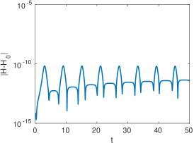
A                                                    B

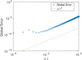
C                                                    D

Figure 10: Three-phase solution: (A) Surface $|u(x,t)|$, (b) error $|H(t)-H(0)|$, (C) global error $|H(50)-H(0)$ and (D) global error $\|u(x,50)-u_{\Delta t}(x,50)\|_{2}$.

Funding

This work was partially supported by Simons Foundation, Grant #527565

References

- [1] A. Osborne, M. Onorato, M. Serio, The nonlinear dynamics of rogue waves and holes in deep-water gravity wave train, Phys. Lett. A 275 (2000) 386–393.
- [2] A. Calini, C. M. Schober, Homoclinic chaos increases the likelihood of rogue wave formation, Phys. Lett. A 298 (2002) 335–349.
- [3] N. N. Akhmediev, J. M. Soto-Crespo, A. Ankiewicz, Extreme waves that appear from nowhere: on the nature of rogue waves, Phys. Lett. A 373 (2009) 2137–2145.
- [4] N. N. Akhmediev, V. M. Eleonskii, N. E. Kulagin, Exact first-order solutions of the nonlinear Schrödinger equation, Theor. Math. Phys. (USSR) 72 (1987) 809–818.
- [5] A. Calini, C. M. Schober, Characterizing JONSWAP rogue waves and their statistics via inverse spectral data, Wave Motion 71 (2017) 5–17.
- [6] J. Chen, D. Pelinovsky, Rogue periodic waves of the focusing nonlinear Schrödinger equation, Proc. Roy. Soc. A 474 (2018).
- [7] J. Chen, D. E. Pelinovsky, R. E. White, Rogue waves on the double-periodic background in the focusing nonlinear Schrödinger equation, Phys. Rev. E 100 (2019).
- [8] A. Calini, C. M. Schober, Numerical investigation of stability of breather-type solutions of the nonlinear Schrödinger equation, Nat. Haz. and Earth Sys. Sci. 14 (2014) 1431–1440.
- [9] M. J. Ablowitz, B. M. Herbst, C. M. Schober, Computational chaos in the nonlinear Schrödinger equation without homoclinic crossings, Physica A 228 (1996) 212 - 235.
- [10] M. G. Forest, C. G. Goedde, A. Sinha, Chaotic transport and integrable instabilities in a near-integrable, many-particle, Hamiltonian lattice, Physica D: Nonlinear Phenomena 67 (1993) 347–386
- [11] A. Calini, N. M. Ercolani, D. W. McLaughlin, C. M. Schober, Mel’nikov analysis of numerically induced chaos in the nonlinear Schrödinger equation, Physica D 89 (1996) 227–260.
- [12] P. G. Grinevich, P. M. Santini, The linear and nonlinear instability of the Akhmediev breather, Nonlinearity 34 (2021).
- [13] K. B. Dysthe, Note on modification to the nonlinear Schrödinger equation for application to deep water waves, Proc. Roy. Soc. Lond. A 369 (1979) 105–114.
- [14] J. D. Carter, D. Henderson, I. Butterfield, A comparison of frequency downshift models of wave trains on deep water, Phys. Fluids 31 (2019).
- [15] K. Trulsen, K. Dysthe, Frequency down-shift in three-dimensional wave trains in a deep basin, J. Fluid Mech. 352 (1997).
- [16] T. Hara, C. Mei, Frequency downshift in narrow banded surface waves under the influence of wind, J. Fluid Mech. 230 (1991) 429–477.
- [17] K. Dysthe, K. Trulsen, H. Krogstad, H. Socquet-Juglard, Evolution of a narrow band spectrum of random surface gravity waves, J. Fluid Mech. 478 (2003) 1–10.
- [18] C. M. Schober, M. Strawn, The effects of wind on nonlinear damping on rogue waves and permanent downshift, PhysicaD 313 (2015) 81–98.
- [19] N. Ercolani, M. G. Forest, D. W. McLaughlin, Geometry of the Modulational Instability III. Homoclinic Orbits for the Periodic sine–Gordon Equation, Physica D 43 (1990) 349 – 384.
- [20] D. W. McLaughlin, E. A. Overman, Whiskered tori for integrable pdes and chaotic behavior in near integrable pdes, Surv. Appl. Math. 1 (1995) 83–203.
- [21] C. M. Schober, A. L. Islas, On the stabilization of breather-type solutions of the damped higher order nonlinear Schrödinger, Front. Phys. 9 (2021).
- [22] V. E. Zakharov, A. B. Shabat, Exact theory of two-dimensional self-focusing and one dimensional self-modulation of waves in nonlinear media, Soviet Phys. JETP 34 (1972) 62–69.
- [23] D. H. Sattinger, V. D. Zurkowski, Gauge theory of bäcklund transformations. ii, Physica D 26 (1987) 225–250.
- [24] M. J. Ablowitz, P. A. Clarkson, Solitons, Nonlinear Evolution Equations and Inverse Scattering Transform, Cambridge University Press, Cambridge, 1991.
- [25] J. E. Prilepsky, S. A. Derevyanko, Breakup of a multisoliton state of the linearly damped nonlinear Schrödinger equation, Phys. Rev. E 75 (2007).
- [26] E. A. Overman, D. W. McLaughlin, A. R. Bishop, Coherence and chaos in the driven damped sine-gordon equation: measurement of the soliton spectrum, Physica D 19 (1986) 1–41.
- [27] C. M. Schober, A. L. Islas, The routes to stability of spatially periodic solutions of the linearly damped nonlinear Schrödinger equation, The European Physical Journal Plus 135 (2020) 1–20.
- [28] A.Q.M. Khaliq, J. Martin-Vaquero, B.A. Wade, M. Yousuf, Smoothing schemes for reaction-diffusion systems with nonsmooth data, Journal of Computational and Applied Mathematics 223 (2009) 374–386.
- [29] X. Liang, A. Q. M. Khaliq, Y. Xing, Fourth order exponential time differencing method with local discontinuous Galerkin approximation for coupled nonlinear Schrödinger equations, Communications in Computational Physics 17 (2015), 510-541
- [30] M. Hederi, A. L. Islas, K. Reger, C. M. Schober, Efficiency of exponential time differencing schemes for nonlinear Schrödinger equations, Mathematics and Computers in Simulation 127 (2016) 101-113
- [31] A. Calini, C. M. Schober, Observable and reproducible rogue waves, J. of Optics, 15 (2013) 105201