Gravitational Wave luminosity distance in viscous cosmological models

Abstract

We study the so-called Gravitational Wave luminosity distance-redshift relation $d_{L}^{\,GW}(z)$ during cosmological eras driven by non-perfect fluids. In particular, we show that the presence of a shear viscosity in the energy momentum tensor turns out to be the most relevant effect. Within this scenario, a constant shear viscosity imprints the gravitational wave propagation through a friction term $\delta(z)$ with a uniquely given redshift dependence. This peculiar evolution predicts a specific shape for the ratio $d_{L}^{GW}/d_{L}^{EM}$ which tends to a constant value when the sources are at $z\gtrsim 1$, whereas scales linearly with the shear viscosity at lower redshifts, regardless of the value of $\Omega_{m0}$. According to our final discussion, the predicted redshift dependence $\delta(z)$ provided by a shear viscosity could be tested by upcoming surveys of multi-messenger sources against analogous scenarios provided by some widely studied theories of modified gravity.

1 Introduction

The detection of Gravitational Waves (GWs) from black holes coalescence [1, 2, 3, 4, 5] has opened a new window for exploring new phenomena of interest for astrophysics and cosmology. Moreover, the subsequent detection of GWs emitted by the binary neutron stars [6], associated to the analysis of the electromagnetic (EM) counterpart [7] (in particular $\gamma$-ray burst [8, 9, 10]) led us to the era of the GWs astrophysics and multimessenger cosmology. In this regards, GWs have opened a new window to understand the nature of gravity [11, 12, 13, 14, 15, 16]. Among all these new kinds of observations, the possibility to have an absolute measurement of the luminosity distance of coalescing compact binaries has gained an increasing interest [17]. Indeed, the signal of coalescing binaries combines intrinsic and apparent luminosity in order to have a determination of the luminosity distance (from which the name standard sirens) [18, 19, 20, 21, 22, 23, 24, 25, 26, 27, 28, 29, 30, 31].

On the other hand, detection of signals like GW170817, observed at $z\simeq 0.009$, can be used to constrain deviations from $\Lambda$CDM model for what concerns either the nature of gravity or the features of the sources. One of the most remarkable cases consists of the simultaneous study of electromagnetic and gravitational signals emitted by the same source: this has provided stringent constraints about differences in their speed of propagation [32, 33, 34, 35, 36] which, for instance, ruled out entire classes of models such as scalar-tensor and vector-tensor theories of gravity [32, 34, 35, 36]. Another idea to be mentioned has been proposed in [31], where it has been shown that GWs could be used as an independent tool to study the Hubble-Lemaître diagram. In fact, the localization of the host galaxy for GW170817 allows to determine $H_{0}$ by the gravitational luminosity distance whereas the electromagnetic counterpart provides the redshift. Another interesting but futuristic idea regards the possibility to study different messengers from the same source through the so-called time-of-flight distance [37, 38].

The different nature of the gravitational signals can shed light on the structure and the evolution of the universe up to early epochs (from the inflationary period to the recombination) that we are unable to probe directly using EM waves. However, for “near” sources, in the next future we could be able to compare both EM and GW signals. It is known that distances in astronomy are calibrated using different techniques, the so-called distance ladder. For near astronomical objects ($z\approx 1$), measurements are usually done using the so called Standard Candles (Supernova IA), from which the accelerated expansion of the universe was firstly observed in 1998 [39]. It is possible to use also binary mergers as standard sirens, which could emit GW and also EM when probably one of the objects is a neutron star. These events are known as Ultranovas and Kilonovas and in [40] it is argued how the latter can be standardized (like Supernova IA) and how the analysis of the distance given by the GW measurements (which does not rely on any distance ladder nor cosmological model), with the redshift, given by the EM counterpart, might provide new probes for measuring the Hubble constant $H_{0}$. For the sake of completeness, we mention also the possibility that a GW can be emitted by a source without an EM counterpart. These sources are the so called dark sirens and their use for the estimation of cosmological parameters is nowadays largely increasing [41].

In this work we discuss how these new observational probes can be investigated to detect modifications on the gravitational luminosity distance as provided by a cosmological viscous fluid. Indeed, the idea that viscosity might play a role in the cosmological dynamics has been discussed already in the middle 60’s [42], where its presence was originally addressed to the gravitational radiation (see also the pioneering works [43, 44, 45, 46]). Recently, the renewed interest in cosmological viscous fluids has increased for different reasons. An interest in the damping of GWs due to the free streaming of neutrinos has been discussed already in the early years of 21st century [47]. However, in this work the focus was in the primordial spectrum of tensor perturbations. In this work, we rather focus on GWs as emitted in the late time Universe.

The most agnostic reason to allow for the presence of viscous fluids is that the perfect fluid description might be a simplistic approximation of the actual Universe. Physically, the emergence of a viscosity might occur in particular scenarios where interaction among the fluids relaxes the thermal equilibrium. According to the specific model in mind, viscosity has been investigated on very early (examining the viscosity effects on the various inflationary observables [48]) and late-time Universe [49].

Clearly, different kind of viscosity can be considered and the specific nature depends on the particular physical mechanims invoked in the cosmic dynamics. As regards the bulk viscosity, it might play an interesting role in the Universe evolution [50, 51, 52, 53], since it is compatible with the symmetry requirements of the homogeneous and isotropic FLRW models. From the theoretical point of view, the bulk viscosity may be due to the deviation from the local thermodynamic equilibrium: in this context, the presence of bulk viscosity would lead to an effective pressure in order to restore the thermal equilibrium, broken by the cosmological fluid expanding (or contracting) too much quick. According to this view, hence the effective pressure due to the bulk viscosity would reduce to the "standard" pressure given by the EoS of a perfect fluid as soon as the fluid itself reaches the equilibrium condition. Also the Dark Energy may be connected with viscosity in the Universe. For instance, [52] studies the possibility that the present acceleration of the universe might be driven by a kind of bulk viscous fluid. However, despite the role of a bulk viscosity might be of interest, along this work we will not consider it, since a bulk viscosity does not lead to an GW attenuation [54, 55, 56].

On the other hand, we will consider the viscosity in the form of a shear one since it affects directly the evolution of tensor perturbations, leaving the background unaltered. The reason for this choice is that we do not want to study a particular model exhibiting a kind of viscosity but we aim to understand which general features can be understood about the viscous model by analysing the GWs evolution.

For the sake of completeness, we mention that the interest in the shear viscosity occurs in some particular scenarios such as the Self Interacting Dark Matter (SIDM) model. Indeed, the SIDM model is able to generate the shear viscosity in the Universe [55, 53, 57] and explain some features in the small scale structure. More generally, other studies consider Viscous Dark Matter where only shear viscosity is considered (see for example [58]).

Having this in mind, the machinery that we will adopt to our ends is in line with to the one developed for the study of the GWs distance-redshift relation concerning theories of modified gravity [59, 60, 61]. The key aspect that we will show is that a viscous fluid can provide a non-trivial ratio between the GW and the EM luminosity distance already within the $\Lambda$CDM model. This interesting aspect emerges when a pure shear viscosity is considered in the cosmic fluid. Indeed, such a modification of the perfect fluid description leaves unchanged the Friedmann equations but can affect the linear part of the perturbations related to the Weyl components of the Riemann tensor, as one would expect by a traceless perturbations of the energy-momentum tensor like a shear viscosity.

After having discussed the general framework for the GWs luminosity distance in the above-mentioned scenario, we will discuss possible observational tests and forecasts for the detection/exclusion of the shear viscosity, according to the specifics of futuristic surveys, such as LISA and Einstein Telescope (ET).

This paper is organized as follows: in Sect. 2, we recall the evolution equation for linear gravitational waves in presence of viscous fluids and provide the general expression for $d_{L}^{\,GW}(z)$. In Sect. 3, we first study our results with a generic power-law solution for the scale factor. Hence we provide an analytical expression for $d_{L}^{\,GW}(z)$ in presence of a shear viscosity in a $\Lambda$CDM-like cosmological model. Possible observational tests and forecasts regarding the presence of shear viscosity are discussed in Sect. 4. Conclusions and discussions are finally provided in Sect. 5.

Conventions: in this paper we will use the metric signature $g_{\mu\nu}=\text{diag}(+,-,-,-)$; the Riemann tensor is defined as $R_{\mu\nu\alpha}\,^{\beta}=\partial_{\mu}\Gamma_{\nu\alpha}\,^{\beta}+\Gamma_{\mu\rho}\,^{\beta}\Gamma_{\nu\alpha}\,^{\rho}-\left(\mu\leftrightarrow\nu\right)$, the Christoffel symbols as $\Gamma_{\mu\nu}\,^{\alpha}=\frac{1}{2}g^{\alpha\beta}(\partial_{\mu}g_{\nu\beta}+\partial_{\nu}g_{\mu\beta}-\partial_{\beta}g_{\mu\nu})$, the Ricci tensor is given by $R_{\nu\alpha}=R_{\mu\nu\alpha}\,^{\mu}$ and the covariant derivatives act as $\nabla_{\mu}A_{\nu\dots}=\partial_{\mu}A_{\nu}-\Gamma_{\mu\nu}\,^{\alpha}A_{\alpha\dots}+\dots$.

2 The Gravitational Wave luminosity distance in viscous scenarios

Let us suppose to describe the contents of the Universe as a dissipative fluid. From a physical point of view the energy momentum tensor of such fluid must depend on the shear viscosity coefficient $\eta_{V}$ and the bulk viscosity coefficient $\zeta$. By introducing the effective pressure

$$\widetilde{p}=p-\left(\zeta-{2\over 3}\eta_{V}\right)\nabla_{\lambda}u^{\lambda},$$ (2.1)

we have the full energy-momentum tensor of the viscous fluid [62, 63, 64, 65] in the following convenient form (see e.g. [67, 68] for recent discussions)

$$\widetilde{T}_{\alpha\beta}=\left(\rho+\widetilde{p}\right)u_{\alpha}u_{\beta}-\widetilde{p}\,g_{\alpha\beta}-\eta_{V}\left[u_{\alpha}u^{\rho}\nabla_{\rho}u_{\beta}+u_{\beta}u^{\rho}\nabla_{\rho}u_{\alpha}-\nabla_{\alpha}u_{\beta}-\nabla_{\beta}u_{\alpha}\right],$$ (2.2)

where $u^{\alpha}$ is the time-like fluid four-velocity ($u_{\alpha}u^{\alpha}=1$). The above energy momentum tensor is known to lead to acausal propagation of first order perturbations. Indeed there exists viable alternatives that have been formulated which do not possess this anomaly such as the Muller-Israel-Stewart theories [69, 70, 71] that are compatible with our expression for the viscous energy momentum tensor when the microscopic relaxation time is much smaller than the time of the macroscopic dissipative process [65], so we will assume this hypothesis throughout the work since we are not considering any particular microphysical model. Moreover even in MIS theories it is not known if causality is preserved under general initial conditions beyond the linear regime [72] and generalized theories are being developed [72, 73]. Despite the above mentioned critical aspect of viscous hydrodynamics, it is customary to describe SIDM as a viscous fluid in terms of a first order gradient expansion as the one we used [53, 74]. For the purposes of this work, we will only consider the presence of shear viscosity $\eta_{V}$. This is a simple but interesting case study since only a bulk viscosity can modify the isotropic background equations (see [56]). Hence, neglecting its presence will allow us to study the GWs propagation by using the standard solutions for the background expansion.

Having this in mind, in this section we will analyze what physical consequences arise from the presence of a shear viscous component in the stress-energy tensor of the cosmological matter fluid: more precisely, we will study how the gravitational luminosity distance is affected and how the gravitational waves propagates in this background. The presence of a shear viscous source introduces an additional friction term in the standard gravitational wave equation in an Friedmann-Lemaître-Robertson-Walker (FLRW) universe, so we expect that the overall differences will be in an increased damping effect of the GW amplitude. We start from the results of Sect. 3.3 of [56]. It has been shown there that the perturbed Einstein-Hilbert action and the energy momentum tensor of a comoving viscous fluid to the second order in the metric, for a conformal FLRW background metric

$$g^{FLRW}_{\mu\nu}=a^{2}(\eta)\text{diag}\left(1,-1,-1,-1\right)\,,$$

and by making use of the TT gauge, leads to the following propagation equation for the tensor perturbations

$${h^{\prime\prime}_{i}}^{\,j}+2\left(\mathcal{H}+\lambda_{p}^{2}\,\eta_{V}\,a\right)\,{h^{\prime}_{i}}^{\,j}-\nabla^{2}{h_{i}}^{j}=0\,,$$ (2.3)

where $\lambda^{2}_{p}=8\pi G$, $\mathcal{H}=a^{\prime}/a$, the prime is referred to derivative with respect to conformal time $\eta$, $\nabla^{2}=\delta^{ij}\partial_{i}\partial_{j}$ and $a(\eta)$ is the FLRW scale factor.

To lighten the notation, let us define $\alpha=\lambda_{p}^{2}\,\eta_{V}$ as the viscosity parameter. We remark that $\alpha$ is a dimensional quantity, scaling as an inverse length. It is worth then to compare its value to $H_{0}$, in order to discuss the regimes when shear viscosity could play a role. For instance, interesting physical values for the shear viscosity have been given in [75], where upper-bounds for $\alpha<10^{-2}\,\text{Mpc}^{-1}\approx 50\,H_{0}$ have been given by the GW150914 data analyzed supposing a viscous background and by viscous dark matter in galaxies,. To be mentioned is also the upper bound $\alpha<10^{-6}\,\text{Mpc}^{-1}\approx 5\times 10^{-3}\,H_{0}$, obtained by estimation of the cross section per unit mass mass $\sigma/m$ from Abell 3827 [76] in a self-interaction model of dark matter. For the sake of simplicity, let us then omit the spatial indices in Eq. (2.3) and

$$h^{\prime\prime}+2\mathcal{H\,}\left[1-\delta(\eta)\right]\,h^{\prime}-\nabla^{2}h=0.$$ (2.4)

where, following [59], we have defined $\delta(\eta)\equiv-\alpha\,a\,\mathcal{H}^{-1}$. From Eq. (2.4), we get that the only effect of a shear viscosity is to alter the evolution equation of a gravitational wave by damping its amplitude through the term $\delta(\eta)$. Since the speed of propagation is not modified, we can follow the same procedure outlined in [60] to study the GW luminosity distance, where the authors precisely take into account a modified evolution equation for the GW’s which has the same form of Eq. (2.4). The interesting aspect concerning the viscous model is that the evolution of $\delta$ is fixed. We then recall the main steps in the following.

To this end, it is useful to express $h\left(\eta,\mathbf{x}\right)$ in terms of its Fourier transform defined as follows

$$h\left(\eta,\mathbf{\mathbf{x}}\right)=\frac{1}{(2\pi)^{3}}\int d^{3}k\,e^{i\mathbf{k}\cdot\mathbf{x}\,}h_{\mathbf{k}}\left(\eta\right).$$ (2.5)

From Eq. (2.4) we obtain the time evolution equation for each mode $k$

$$h_{k}^{\prime\prime}+2\mathcal{H\,}h_{k}^{\prime}+2\alpha\,a\,h_{k}^{\prime}+k^{2}\,h_{k}=0,$$ (2.6)

where we denote $k=|\mathbf{k}|$ and assume $h_{\mathbf{k}}\left(\eta\right)=h_{k}\left(\eta\right)$. It is convenient to rewrite Eq. (2.6) by introducing a new auxiliary variable $v_{k}(\eta)$ as

$$v_{k}\left(\eta\right)\equiv\widetilde{a}(\eta)\,h_{k}(\eta),$$ (2.7)

where we required that the friction term proportional to $v^{\prime}_{k}(\eta)$ in the evolution equation for $v_{k}(\eta)$ is null. Substituting Eq. (2.7) in Eq. (2.6), we are left with two coupled evolution equations for $v_{k}$ and $\widetilde{a}$

$$\begin{cases}v_{k}^{\prime\prime}+\left(k^{2}-\frac{\widetilde{a}^{\prime\prime}}{\widetilde{a}}\right)\,v_{k}=0\\ \frac{\widetilde{a}^{\prime}}{\widetilde{a}}=\mathcal{H}+\alpha\,a\,.\end{cases}$$ (2.8)

Interestingly, first of Eq. (2.8) shows that $v_{k}(\eta)$ behaves as the canonical Mukhanov variable where $\tilde{a}(\eta)$ plays the role of the so-called pump field. Eqs. (2.8) clearly show that GWs in presence of shear viscosity couple to an effective scale factor which fully encodes the viscous content. First of Eqs. (2.8) also shows that on small scales, when $k^{2}\gg\tilde{a}^{\prime\prime}/\tilde{a}$, $v_{k}$ propagates as free-wave. From Eq. (2.7), we then conclude that $h_{k}$ oscillates as well but its amplitude scales as $\tilde{a}^{-1}$.

On the other hand, general relativistic light-like geodesics in a FLRW geometry are not affected by the presence of shear viscosity. Hence, the photon wave-vector scales as $a^{-1}$ [59, 60, 61, 15]. It follows that we can directly apply the same results for the GW luminosity-distance relation already discussed for modified gravity theories. We then have

$$\frac{d_{L}^{GW}}{d_{L}^{EM}}\left(z\right)=\frac{a\left(\eta\right)}{\widetilde{a}\left(\eta\right)},$$ (2.9)

where the equality is obtained by imposing $\widetilde{a}\left(\eta_{0}\right)=a\left(\eta_{0}\right)=\widetilde{a}_{0}=a_{0}$ as initial condition in Eq. (2.8).

Strictly speaking, Eq. (2.9) is fully meaningful when $k^{2}\gg\tilde{a}^{\prime\prime}/\tilde{a}$, where we can write

$$\frac{\tilde{a}^{\prime\prime}}{\tilde{a}}=\frac{a^{\prime\prime}}{a}+3\,\alpha\,a\mathcal{H}+\alpha^{2}a^{2}\,.$$ (2.10)

Moreover, the GWs that we can actually probe propagates on sub-horizon scales. This condition gives $k\eta\gg 1$ for a class of cosmological models such as power-law scale factor or $\Lambda$CDM, where it also holds $a^{\prime\prime}/a\sim\eta^{-2}$ and $\mathcal{H}\sim\eta^{-1}$. This means that the requirement $k^{2}\gg\tilde{a}^{\prime\prime}/\tilde{a}$ translates to

$$\left(\frac{k}{\mathcal{H}}\right)^{2}\gg 1+3\,a\,\frac{\alpha}{\mathcal{H}}+a^{2}\,\left(\frac{\alpha}{\mathcal{H}}\right)^{2}\,.$$ (2.11)

Since $a<1$, for the redshift of interest for upcoming observations such as LISA [79, 80] and ET [81], i.e. $z\lesssim 2$, Eq. (2.11) tells us that sub-horizon modes can be safely considered for our models as long as $\alpha\,H^{-1}_{0}\lesssim 1$. Instead, for higher values of $\alpha$ our results are meaningful for $k\gg\alpha$. It is worth to remark that when $\alpha\gtrsim H_{0}$, not all the subhorizon modes are compatible with our discussion, since the scale introduced by $\alpha$ lays within the horizon itself. However, our analysis is still viable for the range of wavelengths compatible with the current and forthcoming interferometers. Indeed, for the case of quite large shear viscosity $\alpha=10H_{0}$, we would have that the spatial scale of $\alpha^{-1}$ is roughly 10 times smaller than the horizon. This scale is anyway much larger than the wavelength range that Earth and Space based interferometers are able to probe, ensuring then that the condition $k\gg\alpha$ is always safely satisfied for the modes of our interest.

In the following sections we will discuss the explicit cases for a power-law scale factor and for the $\Lambda$CDM model.

3 Viscous models

In this section, we study the GW distance-redshift relation for some particular cases of physical interest. Firstly, we analyze the case of a generic power law behaviour for the scale factor. An interesting application for this case could provided by models where also the bulk viscosity is not null. Indeed, in this case the Friedmann equations are modified by the bulk viscosity and some interesting deviation from the Cosmic Concordance model might occur. Secondly, we will discuss the case of a viscous extension of $\Lambda$CDM model, where only shear viscosity is allowed.

3.1 Power-law solution

We first present the illustrative case of a power-law solution for the cosmological background. Under these assumptions, the scale factor in term of the conformal time $\eta$ reads

$$a\left(\eta\right)=a_{0}\left(\frac{\eta}{\eta_{0}}\right)^{\beta},$$ (3.1)

and this yields to $\mathcal{H}=\frac{\beta}{\eta}$, where $\eta_{0}$ is the conformal time today. Inserting the last two equalities in the second line of Eq. (2.8) we then have

$$\frac{\widetilde{a}^{\prime}}{\widetilde{a}}=\frac{\beta}{\eta}+\alpha\,a_{0}\left(\frac{\eta}{\eta_{0}}\right)^{\beta}$$ (3.2)

with the initial condition given by $\widetilde{a}\left(\eta_{0}\right)=a\left(\eta_{0}\right)$. We have done this choice in order to recover $d_{L}^{\,GW}(0)=d_{L}^{\,EM}(0)$ (see Eq. (2.9). For $\beta\neq-1$, we then have

$$\widetilde{a}\left(\eta\right)=a(\eta)\exp\left[\frac{\alpha\,a_{0}\left(\eta^{\beta+1}-\eta_{0}^{\beta+1}\right)}{(\beta+1)\eta_{0}^{\beta}}\right].$$ (3.3)

A direct comparison between Eqs. (3.1) and (3.3) shows that the damping effects introduced by the shear viscosity is an exponential suppression in the past of the effective scale factor $\tilde{a}$, which governs the GWs propagation.

Finally, we substitute Eq. (3.3) in Eq. (2.9) to obtain

$$\frac{d_{L}^{GW}\left(\eta\right)}{d_{L}^{EM}\left(\eta\right)}=\exp\left\{\frac{\alpha\,a_{0}\eta_{0}}{(\beta+1)}\left[1-\left(\frac{a}{a_{0}}\right)^{(\beta+1)/\beta}\right]\right\}\,.$$ (3.4)

Since our observations relate distances to redshift, the last equation (3.4) can be further manipulated in order to make explicit the dependence on $z$. To this purpose, we first recall that $1+z=\frac{a_{0}}{a}$. Hence by expressing the conformal time today in terms of the Hubble constant $H_{0}$ we obtain

$$\frac{d_{L}^{GW}}{d_{L}^{EM}}\left(z\right)=\text{exp}\left[\frac{\beta}{\beta+1}\frac{\alpha}{H_{0}}\left(1-\frac{1}{\left(1+z\right)^{\frac{\beta+1}{\beta}}}\right)\right]\,.$$ (3.5)

This is the most general equation that relates the gravitational luminosity distance to the redshift in a power law Universe with constant shear viscosity. Setting $\beta=2$, we apply the general result given in Eq. (3.5) to the physical scenario of a matter dominated Universe (Einstein-de Sitter Universe). In Fig. 1 we show the relative correction between the gravitational and the electromagnetic luminosity distance-redshift relation as given by Eq. (3.5) for different values of viscosities.

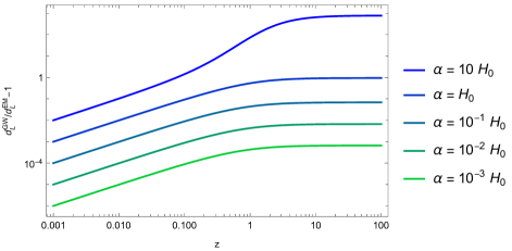
Figure 1: Luminosity distance ratio for different values of $\alpha$ in unit of $H_{0}$ for CDM model.

Regardless of the value of $\alpha$, we notice that all the solutions tend to a constant value of the ratio beyond a certain redshift $z^{*}$. For a generic value of $\beta$, this overall offset is given by

$$\frac{d_{L}^{GW}}{d_{L}^{EM}}\approx e^{\frac{\alpha}{H_{0}}\frac{\beta}{(\beta+1)}}\,,$$ (3.6)

which clearly shows that is controlled by the ratio $\alpha/H_{0}$. Before moving on, a comment about the behavior for large $\alpha/H_{0}$ in Fig. 1 is in order. The intermediate bump emerging when $\alpha=10\,H_{0}$ is due to the nonlinear modification of $\tilde{a}$ with respect to $a$, as accounted for in the second of Eqs. (2.8). With the proviso that $k^{2}\gg\tilde{a}^{\prime\prime}/\tilde{a}$, $h_{k}$ scales as $\tilde{a}^{-1}$, regardless of $k$. Hence we get that the scaling of the GW amplitude is entirely given by Eq. (3.5), as a consequence of the second of Eqs. (2.8). When $\alpha\ll H_{0}$, Eq. (3.5) gives

$$\frac{d^{GW}_{L}}{d^{EM}_{L}}(z)=1+\frac{\alpha}{H_{0}}\frac{\beta}{\beta+1}\left[1-\left(1+z\right)^{-\frac{\beta+1}{\beta}}\right]+\mathcal{O}\left(\left(\frac{\alpha}{H_{0}}\right)^{2}\right)\,,$$ (3.7)

which only exhibits two regimes when $z$ is compared to 1. However, when $\alpha\gtrsim H_{0}$, the nonlinear dependence of $d^{GW}_{L}/d^{EM}_{L}$ cannot be neglected. In particular, since both small ($z\ll 1$) and large ($z\gg 1$) redshift behaviors are universal in regard to the value of $\alpha H^{-1}_{0}$, the intermediate range at $z\sim 1$ is precisely the only range where the nonlinear dependence on the shear viscosity can change the qualitative form of Fig. 1.

Although an Einstein-de Sitter universe is a very good approximation of the evolution of the Universe after the CMB, it fails to reproduce the recent Dark Energy epoch and a better model of the Universe is required. In the next subsection we will discuss the effects of viscosity within a $\Lambda$CDM-like model.

3.2 A viscous $\Lambda$CDM model

After recombination, the radiation contribution to the expansion of the Universe has become negligible. Ignoring the radiation component may underestimate observables related to the primordial tensor perturbations (such as 2-point correlation of the lensing shear [82]), especially on scales small enough to have re-entered the horizon before the recombination. However, the GW’s analysed with the $d^{GW}_{L}(z)$ are not related to the primordial tensor spectrum, as they are emitted only in recent epochs (up to $z\sim 5$), where the radiation component can be safely neglected.

The first difficulty we have to deal with is the absence of an analytic expression for $a(\eta)$ in the Cosmic Concordance model. In order to circumvent this technical aspect, it is convenient to rewrite the second line of Eq. (2.8) in terms of the redshift. With this in mind, we first provide the following well-known relations ($a_{0}=1$)

$$\frac{d}{d\eta}=-H(z)\frac{d}{dz}\qquad\text{and}\quad\mathcal{H}(z)=\frac{H(z)}{1+z}\,,$$ (3.8)

where

$$H(z)=H_{0}\sqrt{\Omega_{m0}(1+z)^{3}+\Omega_{\Lambda 0}}\,,$$ (3.9)

and clearly $\Omega_{\Lambda 0}+\Omega_{m0}=1$. Therefore, first of Eqs. (2.8) becomes

$$\frac{d\ln\widetilde{a}}{dz}=-\frac{1}{1+z}-\frac{\alpha(z)}{H(z)(1+z)}\,.$$ (3.10)

By integrating the lhs between $\widetilde{a}_{0}=a_{0}=1$ and $\widetilde{a}$ and the rhs between 0 and $z$ we obtain

$$\widetilde{a}(z)=\frac{1}{1+z}\exp\left(-\int_{0}^{z}\frac{\alpha(z^{\prime})}{(1+z^{\prime})H(z^{\prime})}dz^{\prime}\right)\,,$$ (3.11)

Once inserted in Eq. (2.9), Eq. (3.11) gives

$$\frac{d_{L}^{GW}}{d_{L}^{EM}}\left(z\right)=\text{exp}\left[\int_{0}^{z}\frac{\alpha(z^{\prime})}{(1+z^{\prime})H(z^{\prime})}dz^{\prime}\right].$$ (3.12)

Last equation is a general expression that holds true in any FLRW cosmology with a viscous fluid component in the stress-energy tensor, where the shear viscosity parameter is not constant. All the information about the background gravitational sources is encoded in $H(z)$.

We remark that Eq. (3.12) holds true also for values of $H(z)$ which are more general of Eq. (3.9). Indeed, as long as the Hubble function is evaluated accordingly to the total stress-energy tensor, it follows that the equation is valid even if the fluids do not have a barotropic equation of state (e.g. polytropic fluids) and it remains valid also in the presence of bulk viscous contributions. However, since now on, we will only consider background dynamics driven by dark matter and $\Lambda$, in agreement with the value of $H(z)$ provided in Eq. (3.9).

With this in mind, we then combine Eq. (3.12) and with Eq. (3.9) and consider a constant $\alpha(z)=\alpha$. We underline that the shear viscous parameter $\alpha$ in a model with a mixture of viscous fluids is given by $\alpha=\sum_{A}\alpha_{A}$, where $A$ is an index that runs over the different viscous fluids. As a consequence, with this condition, in a $\Lambda$CDM-like model it is not possible to distinguish which fluid component between Dark Energy, Dark Matter or both is responsible for the shear viscous effects on the gravitational wave propagation. However, if one has in mind a minimal extension to the $\Lambda$CDM model, the viscous property should be addressed only to the Dark Matter fluid. This is because a Dark Energy as given by a cosmological constant is the only term compatible with General Relativity, according to the hypothesis of the Lovelock theorem. This minimal description admits then an EoS for $\Lambda$ which is nothing but the one of a perfect fluid. The integral in Eq. (3.12) hence becomes

$$\int_{0}^{z}\frac{1}{(1+z^{\prime})H(z^{\prime})}dz^{\prime}=\frac{1}{3H_{0}\sqrt{\Omega_{\Lambda 0}}}\ln\left(\frac{H(z)/H_{0}-\sqrt{\Omega_{\Lambda 0}}}{H(z)/H_{0}+\sqrt{\Omega_{\Lambda 0}}}\,\frac{1+\sqrt{\Omega_{\Lambda 0}}}{1-\sqrt{\Omega_{\Lambda 0}}}\right)$$ (3.13)

bringing then to

$$\frac{d_{L}^{GW}}{d_{L}^{EM}}\left(z\right)=\left(\frac{\sqrt{\Omega_{m0}(1+z)^{3}+\Omega_{\Lambda 0}}-\sqrt{\Omega_{\Lambda 0}}}{\sqrt{\Omega_{m0}(1+z)^{3}+\Omega_{\Lambda 0}}+\sqrt{\Omega_{\Lambda 0}}}\,\frac{1+\sqrt{\Omega_{\Lambda 0}}}{1-\sqrt{\Omega_{\Lambda 0}}}\right)^{\frac{\alpha}{3H_{0}\sqrt{\Omega_{\Lambda 0}}}}\,.$$ (3.14)

Just as discussed in the previous section, we have again a critical redshift $z^{*}$ such that, when $z>z^{*}$, we have:

$$\Xi_{0}\equiv\frac{d_{L}^{GW}}{d_{L}^{EM}}(z\gg z^{*})=\left(\frac{1+\sqrt{\Omega_{\Lambda 0}}}{1-\sqrt{\Omega_{\Lambda 0}}}\right)^{\frac{\alpha}{3H_{0}\sqrt{\Omega_{\Lambda 0}}}}\,.$$ (3.15)

Here we have called this limit value $\Xi_{0}$ since we have in mind the widely used parametrization of $d_{L}^{\,GW}/d_{L}^{\,EM}$ proposed in [60]

$$\frac{d_{L}^{\,GW}}{d_{L}^{\,EM}}(z)=\Xi_{0}+\frac{1-\Xi_{0}}{(1+z)^{n}}\,.$$ (3.16)

According to Eq. (3.14), the parametrization in Eq. (3.16) is not expected to work perfectly for any value of $\alpha$.

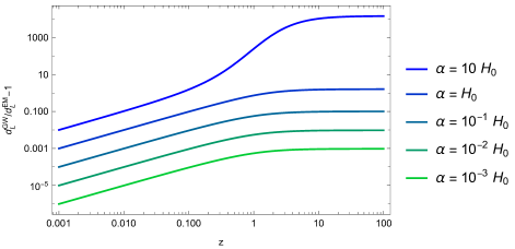
Figure 2: Luminosity distance ratio for different values of $\alpha$ in unit of $H_{0}$ for $\Lambda$CDM where $\Omega_{m0}=0.307$ has been taken in accordance to the local estimation from the Pantheon sample [84].

Indeed, as we can see from Fig. 2, for high value of $\alpha/H_{0}$, the emergence of an intermediate slope at redshifts $\sim 1$ renders Eq. (3.16) hard to be used. However, when $\alpha$ is perturbatively smaller than $H_{0}$, Eq. (3.16) works quite well.

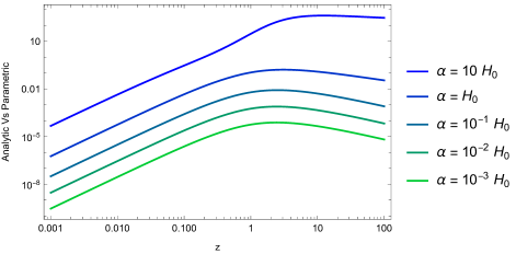
Figure 3: Relative error between the exact expression in Eq. (3.14) and the parametric expression in Eq. (3.16). We fix $\Omega_{m0}=0.307$ in accordance to the local estimation of the Pantheon sample [84]. This plot shows that the widely used parametrization in Eq. (3.16) is reliable only for small values of $\alpha\,H^{-1}_{0}$.

This is more evident in Fig. 3, where the slope $n$ in Eq. (3.16) has been modeled as (see [85] for a detailed discussion about different parametrization of $n$)

$$n\equiv\frac{\delta(0)}{1-\Xi_{0}}\,.$$ (3.17)

The dependences of $\Xi_{0}$ and $n$ on the ratio $\alpha/H_{0}$ are shown in Fig. 4, where $\Omega_{m0}=0.307$ has been taken in accordance to [84].

Figure 4: Dependence of $\Xi_{0}$ (left) and $n$ (right) in terms of $\alpha H^{-1}_{0}$, according to the widely used parametrization given in Eq. (3.16). The value of $\Omega_{m0}=0.307$ has been taken in accordance to the local estimation from the Pantheon sample [84].

From both these panels, we notice that the discrepancy between the gravitational and electromagnetic luminosity distance deviates exponentially when the shear viscosity becomes of order of $H_{0}$.

What emerges from Figs. 3 and 4 is that the parametrization of Eq. (3.16) can be safely adopted also for the viscous models when its value is at maximum of few percent of the $H_{0}$. Accordingly, also the constraints on the value of $\alpha$ from Eq. (3.16) are not trustworthy beyond this regime. The reason for this discrepancy stands in the fact that Eq. (3.16) holds when $d_{L}^{\,GW}/d_{L}^{\,EM}$ exhibits only two regimes: top curve of Fig. 2 clearly shows that this is not the case when $\alpha\gg H_{0}$. We remark that in this case the estimation of $n$ becomes meaningless whereas $\Xi_{0}$ can still be interpreted as the limit value of $d_{L}^{\,GW}/d_{L}^{\,EM}$.

As a final remark we show that in the limit $\Omega_{\Lambda 0}\rightarrow 0$ we retrieve the Einstein-de Sitter solution given in Eq. (3.5) by setting $\beta=2$. To this end, it is more straightforward to expand in terms of $\Omega_{\Lambda 0}$ Eq. (3.13), having in mind the constraint $\Omega_{m0}=1-\Omega_{\Lambda 0}$. Since we are interested in the leading term and the logarithm is divided $\sqrt{\Omega_{\Lambda 0}}$, we neglect terms of order $\mathcal{O}(\Omega_{\Lambda 0})$ or higher. First fraction in the argument of the logarithm of Eq. (3.13) then becomes

$$\frac{\sqrt{\Omega_{m0}(1+z)^{3}+\Omega_{\Lambda 0}}-\sqrt{\Omega_{\Lambda 0}}}{\sqrt{\Omega_{m0}(1+z)^{3}+\Omega_{\Lambda 0}}+\sqrt{\Omega_{\Lambda 0}}}= \frac{\sqrt{1-\Omega_{\Lambda 0}+\Omega_{\Lambda 0}(1+z)^{-3}}-\sqrt{\Omega_{\Lambda 0}}(1+z)^{-3/2}}{\sqrt{1-\Omega_{\Lambda 0}+\Omega_{\Lambda 0}(1+z)^{-3}}+\sqrt{\Omega_{\Lambda 0}}(1+z)^{-3/2}}$$

$$= \frac{1-\sqrt{\Omega_{\Lambda 0}}(1+z)^{-3/2}}{1+\sqrt{\Omega_{\Lambda 0}}(1+z)^{-3/2}}+\mathcal{O}\left(\Omega_{\Lambda 0}\right)$$

$$= 1-2\,\sqrt{\Omega_{\Lambda 0}}\,(1+z)^{-3/2}+\mathcal{O}\left(\Omega_{\Lambda 0}\right)\,.$$ (3.18)

In the same way, for the second fraction in Eq. (3.13) we have

$$\frac{1+\sqrt{\Omega_{\Lambda 0}}}{1-\sqrt{\Omega_{\Lambda 0}}}=1+2\sqrt{\Omega_{\Lambda 0}}+\mathcal{O}(\Omega_{\Lambda 0})\,.$$ (3.19)

Hence, thanks to Eqs. (3.18) and (3.19), the expansion of the logarithm in Eq. (3.13) is

$$\ln\left(\frac{H(z)/H_{0}-\sqrt{\Omega_{\Lambda 0}}}{H(z)/H_{0}+\sqrt{\Omega_{\Lambda 0}}}\,\frac{1+\sqrt{\Omega_{\Lambda 0}}}{1-\sqrt{\Omega_{\Lambda 0}}}\right)=2\sqrt{\Omega_{\Lambda 0}}\left[1-(1+z)^{-3/2}\right]+\mathcal{O}\left(\Omega^{3/2}_{\Lambda 0}\right)\,.$$ (3.20)

By inserting this last expansion in Eq. (3.13), we then arrive at

$$\int_{0}^{z}\frac{1}{(1+z^{\prime})H(z^{\prime})}dz^{\prime}=\frac{2}{3H_{0}}\left[1-(1+z)^{-3/2}\right]+\mathcal{O}\left(\Omega_{\Lambda 0}\right)\,.$$ (3.21)

Finally, by using Eq. (3.12) with a constant $\alpha$, we recover the result of Eq. (3.5).

4 A smoking gun for the shear viscosity?

An interesting feature emerging from the discussion in the previous section is the neat distinction between two regimes of the ratio $d_{L}^{\,GW}/d_{L}^{\,EM}$ for small values of $\alpha/H_{0}$. The crossing from one regime to the other occurs at a given redshift, where a knee between the linear and constant behaviour is evident. To quantify this transition, we first expand Eq. (3.14) for low redshift

$$\frac{d_{L}^{\,GW}}{d_{L}^{\,EM}}=1-\delta(0)\,z+\mathcal{O}\left(z^{2}\right)=1+\frac{\alpha}{H_{0}}z+\mathcal{O}\left(z^{2}\right)\,,$$ (4.1)

where, following [59], we have used $\delta(0)=-\alpha\,H^{-1}_{0}$. It is already interesting to notice from Eq. (4.1) that the linear regime appearing at low redshift of Fig. 2 is independent of $\Omega_{m0}$: a detection of a linear increasing behaviour for close sources is entirely addressed to a non-null shear viscosity in this scenario, regardless of the value of $\alpha$. However, the amplitude still look prohibitive according to the forecasted precision at those redshifts. Indeed, following [60], we can use the the stringent limit on $\delta(0)$ coming from combined observations of the standard siren GW170817 [6] and electromagnetic counterpart of its host galaxy NGC4993 [86, 87]. This provides the bounds $\delta(0)=-7.8^{+9.7}_{-18.4}$. Despite this is a test to directly constrain $\alpha H^{-1}_{0}$, the provided bound is unfortunately not so stringent.

Stronger constraints can be put by considering the forecasts for LISA [85] and ET [60]. To this end, we make use of the parametrization in Eq. (3.16) and consider the forecasted error $\Delta\Xi_{0}$ respectively given by $0.044$ for LISA [85] and $0.008$ for ET [60]. Indeed, for small values of $\alpha H^{-1}_{0}$, Eq. (3.15) gives

$$\Xi_{0}\approx 1+\frac{1}{3}\frac{\alpha}{H_{0}}\ln\left(\frac{1+\sqrt{\Omega_{\Lambda 0}}}{1-\sqrt{\Omega_{\Lambda 0}}}\right)\,.$$ (4.2)

Eq. (4.2) we can then be inverted to get the ratio $\alpha/H_{0}$ as a function of the parameters $\Omega_{m0}$ and $\Xi_{0}$. In this way, the precision on the estimation of $\alpha/H_{0}$ propagating from the error bars of $\Xi_{0}$ and $\Omega_{m0}$ is

$$\Delta\left(\frac{\alpha}{H_{0}}\right)=\frac{3\,\Delta\Xi_{0}}{\ln\left(\frac{1+\sqrt{\Omega_{\Lambda 0}}}{1-\sqrt{\Omega_{\Lambda 0}}}\right)}+\frac{3\,|1-\Xi_{0}|\,\Delta\Omega_{m0}}{\sqrt{\Omega_{\Lambda 0}}\,\Omega_{m0}\ln^{2}\left(\frac{1+\sqrt{\Omega_{\Lambda 0}}}{1-\sqrt{\Omega_{\Lambda 0}}}\right)}\,.$$ (4.3)

Around the fiducial values of the standard cosmic concordance model ($\Xi_{0}=1$), we then have that $\alpha/H_{0}$ could be constrained by future missions with an error given by

$$\Delta\left(\frac{\alpha}{H_{0}}\right)\approx\frac{3\,\Delta\Xi_{0}}{\ln\left(\frac{1+\sqrt{\Omega_{\Lambda 0}}}{1-\sqrt{\Omega_{\Lambda 0}}}\right)}\approx\Delta\Xi_{0}\,,$$ (4.4)

where we have used the value $\Omega_{m0}=0.307\pm 0.012$ as given by the independent estimation from Pantheon sample [84]. We remark that Eq. (4.4) follows from the optimistic case $\Xi_{0}=1$ where the contribution of $\Delta\Omega_{m0}$ to the ultimate forecasts cancels out. However, our result is reliable also for more conservative scenarios. Indeed, if we let $\Xi_{0}$ deviate from 1 by the same order of magnitude permitted by the error bars (namely $|1-\Xi_{0}|\sim\Delta\Xi_{0}$), we get that our forecast in Eq. (4.4) is worsen only by $\sim 1\%$, according to our chosen cosmological parameters.

Interestingly, the forecasted error $\alpha/H_{0}$ is almost of the same order of magnitude as the one for $\Xi_{0}$. This opens a new window to investigate whether a shear viscosity of order of few percents of $H_{0}$ is present in the cosmological fluids. We also remark that these constraints are more stringent than the ones provided by the same analysis for particular classes of modified gravity theories, where the forecasted errors for the free parameters are worsen by almost one order of magnitude wrt to $\Delta\Xi_{0}$ [88].

As a further remark, an interesting idea would be to use Eq. (4.4) as a forecast for $\alpha$ itself, rather than just $\alpha\,H^{-1}_{0}$. This could be achieved by combining Eq. (4.4) with the analysis of the expected Hubble-Lemaître diagram from Superluminous Supernovae [89] for forthcoming Large-Scale Structure surveys at higher redshift (up to $z=4$). Indeed, it has been shown in [90] that this analysis could provide a (model dependent) estimation of $H_{0}$ at a precision level of $\sim 0.1\%$.

Finally, we discuss another test that could be done by looking at the transition between the linear evolution and the constant offset given by Eq. (3.15). This transition would occur at the redshift $z^{*}$ when the linear growth in Eq. (4.1) reaches the offset value in Eq. (3.15). This simple reasoning returns an expression for $z^{*}$ given by

$$z^{*}=\frac{H_{0}}{\alpha}\left[\left(\frac{1+\sqrt{1-\Omega_{m0}}}{1-\sqrt{1-\Omega_{m0}}}\right)^{\frac{\alpha}{3H_{0}\sqrt{1-\Omega_{m0}}}}-1\right]\,.$$ (4.5)

We remark that Eq. (4.5) is meaningful only for small values of the ratio $\alpha/H_{0}$, since the transition between the linear and the constant regime occurs directly only in this case. Indeed, Fig. 2 for values $\alpha/H_{0}>1$, a third intermediate regime appears and this breaks the validity of the discussed case study. Fortunately, the values of $\alpha$ when this limitation occurs are too high to be seriously considered. It is worth to notice that when $\alpha\ll H_{0}$, within the uncertainties of $\Omega_{m0}=0.307\pm 0.012$ given by [84], the value of $z^{*}$ is quite stable around the value of $z^{*}=1$.

5 Conclusions and outlook

In this paper we have studied the influence of shear viscosity on the so-called gravitational luminosity distance. The main property of the shear viscosity is that it leaves unchanged the Friedmann equations and modifies the linear tensor perturbations by an additional friction terms. As a consequence, the most stringent constraints on the speed of GWs propagation are satisfied but a lot of room for other effects can be investigated.

In particular, the friction term $\delta(\eta)$ arising from the viscosity impacts the GW luminosity distance-redshift relation in two specific ways:

• the shear viscosity introduces a new length scale $\alpha$;

• the friction term depends on the Hubble function through the ratio $\alpha/\mathcal{H}$.

From these two properties we infer that the relevant parameter to study and/or discard the presence of the shear viscosity in the cosmological fluid is the relative amplitude between $\alpha$ and $H_{0}$. In this regard, we have shown that when $\alpha H^{-1}_{0}\ll 1$, most of the well known techniques for the study of GW luminosity distance in modified gravity theories can be directly applied.

More specifically, for a $\Lambda$CDM-like viscous model, the gravitational distance given in Eq. (3.14) exhibits a constant asymptotic value at redshifts $z>1$ as given by the parameter $\Xi_{0}$. For the case of perturbative amplitude of $\alpha/H_{0}$, $\Xi_{0}$ can actually be interpreted as usually done [60] for the parametrization of Eq. (3.16) and consequently forecast whether it will be possible to discriminate the presence shear viscosity from futuristic surveys, such as LISA and ET. Our analysis indicates that non-perfect fluids with a shear viscosity could be studied in details up to values of the $\alpha$ of few percents of $H_{0}$.

On the contrary, non-perturbative values of the shear viscosity ($\alpha\gtrsim H_{0}$) could be easily distinguished from all the class of models compatible with Eq. (3.16) and there are two reasons for that:

• first of all, the offset value $\Xi_{0}$ exponentially grows with $\alpha/H_{0}$. This means that a large deviation of $d^{\,GW}_{L}$ from the EM luminosity distance could be easily detectable, if present.

• Secondly, the redshift dependence of $d_{L}^{\,GW}/d_{L}^{\,EM}$ largely differs from the parametric fitting functions in Eq. (3.16), also at intermediate redshifts around $z\sim 1$ (see the curve for $\alpha=10\,H_{0}$ in Fig. 2).

As a final remark, we stress that the behaviour of $d_{L}^{\,GW}/d_{L}^{\,EM}$ for small redshifts ($z\ll 1$), is insensitive to $\Omega_{m0}$ and depends only linearly on the ratio $\alpha/H_{0}$, regardless of its amplitude. For this kind of close sources, the independent estimation of $z$, $d_{L}^{\,EM}$ and $d_{L}^{\,GW}$ may allow to have independent measurements of $H_{0}$ and $\alpha$ rather than just their ratio. This is also likely in view of the use the three-dimensional cross-correlation technique for GWs sources and galaxies [91, 92]. Such a scenario could provide a highly promising test to estimate the shear viscosity if the precision concerning the measurement of $d_{L}^{\,GW}$ would dramatically increase in the next years.

References

- [1] B. P. Abbott et al., Observation of Gravitational Waves from a Binary Black Hole Merger, Phys. Rev. Lett. 116 (2016), no. 6 061102, [arXiv:1602.03837].
- [2] B. P. Abbott et al., GW151226: Observation of Gravitational Waves from a 22-Solar-Mass Binary Black Hole Coalescence, Phys. Rev. Lett. 116 (2016), no. 24 241103, [arXiv:1606.04855].
- [3] B. P. Abbott et al., GW170104: Observation of a 50-Solar-Mass Binary Black Hole Coalescence at Redshift 0.2, Phys. Rev. Lett. 118 (2017), no. 22 221101, [arXiv:1706.01812]. [Erratum: Phys.Rev.Lett. 121, 129901 (2018)].
- [4] B. P. Abbott et al., GW170608: Observation of a 19-solar-mass Binary Black Hole Coalescence, Astrophys. J. Lett. 851 (2017) L35, [arXiv:1711.05578].
- [5] B. P. Abbott et al., GW170814: A Three-Detector Observation of Gravitational Waves from a Binary Black Hole Coalescence, Phys. Rev. Lett. 119 (2017), no. 14 141101, [arXiv:1709.09660].
- [6] B. P. Abbott et al., GW170817: Observation of Gravitational Waves from a Binary Neutron Star Inspiral, Phys. Rev. Lett. 119 (2017), no. 16 161101, [arXiv:1710.05832].
- [7] B. P. Abbott et al., Multi-messenger Observations of a Binary Neutron Star Merger, Astrophys. J. Lett. 848 (2017), no. 2 L12, [arXiv:1710.05833].
- [8] A. Goldstein et al., An Ordinary Short Gamma-Ray Burst with Extraordinary Implications: Fermi-GBM Detection of GRB 170817A, Astrophys. J. Lett. 848 (2017), no. 2 L14, [arXiv:1710.05446].
- [9] V. Savchenko et al., INTEGRAL Detection of the First Prompt Gamma-Ray Signal Coincident with the Gravitational-wave Event GW170817, Astrophys. J. Lett. 848 (2017), no. 2 L15, [arXiv:1710.05449].
- [10] B. P. Abbott et al., Gravitational Waves and Gamma-rays from a Binary Neutron Star Merger: GW170817 and GRB 170817A, Astrophys. J. Lett. 848 (2017), no. 2 L13, [arXiv:1710.05834].
- [11] C. Deffayet and K. Menou, Probing Gravity with Spacetime Sirens, Astrophys. J. Lett. 668 (2007) L143–L146, [arXiv:0709.0003].
- [12] C. M. Will, The Confrontation between General Relativity and Experiment, Living Rev. Rel. 17 (2014) 4, [arXiv:1403.7377].
- [13] N. Yunes, K. Yagi, and F. Pretorius, Theoretical Physics Implications of the Binary Black-Hole Mergers GW150914 and GW151226, Phys. Rev. D 94 (2016), no. 8 084002, [arXiv:1603.08955].
- [14] R.-G. Cai, Z. Cao, Z.-K. Guo, S.-J. Wang, and T. Yang, The Gravitational-Wave Physics, Natl. Sci. Rev. 4 (2017), no. 5 687–706, [arXiv:1703.00187].
- [15] M. Maggiore, Gravitational Waves. Vol. 1: Theory and Experiments. Oxford Master Series in Physics. Oxford University Press, 2007.
- [16] M. Maggiore, Gravitational Waves. Vol. 2: Astrophysics and Cosmology. Oxford University Press, 3, 2018.
- [17] L. Lombriser and A. Taylor, Breaking a Dark Degeneracy with Gravitational Waves, JCAP 03 (2016) 031, [arXiv:1509.08458].
- [18] N. Dalal, D. E. Holz, S. A. Hughes, and B. Jain, Short grb and binary black hole standard sirens as a probe of dark energy, Phys. Rev. D 74 (2006) 063006, [astro-ph/0601275].
- [19] C. L. MacLeod and C. J. Hogan, Precision of Hubble constant derived using black hole binary absolute distances and statistical redshift information, Phys. Rev. D 77 (2008) 043512, [arXiv:0712.0618].
- [20] S. Nissanke, D. E. Holz, S. A. Hughes, N. Dalal, and J. L. Sievers, Exploring short gamma-ray bursts as gravitational-wave standard sirens, Astrophys. J. 725 (2010) 496–514, [arXiv:0904.1017].
- [21] C. Cutler and D. E. Holz, Ultra-high precision cosmology from gravitational waves, Phys. Rev. D 80 (2009) 104009, [arXiv:0906.3752].
- [22] B. S. Sathyaprakash, B. F. Schutz, and C. Van Den Broeck, Cosmography with the Einstein Telescope, Class. Quant. Grav. 27 (2010) 215006, [arXiv:0906.4151].
- [23] W. Zhao, C. Van Den Broeck, D. Baskaran, and T. G. F. Li, Determination of Dark Energy by the Einstein Telescope: Comparing with CMB, BAO and SNIa Observations, Phys. Rev. D 83 (2011) 023005, [arXiv:1009.0206].
- [24] W. Del Pozzo, Inference of the cosmological parameters from gravitational waves: application to second generation interferometers, Phys. Rev. D 86 (2012) 043011, [arXiv:1108.1317].
- [25] A. Nishizawa, K. Yagi, A. Taruya, and T. Tanaka, Cosmology with space-based gravitational-wave detectors — dark energy and primordial gravitational waves —, Phys. Rev. D 85 (2012) 044047, [arXiv:1110.2865].
- [26] S. R. Taylor and J. R. Gair, Cosmology with the lights off: standard sirens in the Einstein Telescope era, Phys. Rev. D 86 (2012) 023502, [arXiv:1204.6739].
- [27] S. Camera and A. Nishizawa, Beyond Concordance Cosmology with Magnification of Gravitational-Wave Standard Sirens, Phys. Rev. Lett. 110 (2013), no. 15 151103, [arXiv:1303.5446].
- [28] N. Tamanini, C. Caprini, E. Barausse, A. Sesana, A. Klein, and A. Petiteau, Science with the space-based interferometer eLISA. III: Probing the expansion of the Universe using gravitational wave standard sirens, JCAP 04 (2016) 002, [arXiv:1601.07112].
- [29] C. Caprini and N. Tamanini, Constraining early and interacting dark energy with gravitational wave standard sirens: the potential of the eLISA mission, JCAP 10 (2016) 006, [arXiv:1607.08755].
- [30] R.-G. Cai and T. Yang, Estimating cosmological parameters by the simulated data of gravitational waves from the Einstein Telescope, Phys. Rev. D 95 (2017), no. 4 044024, [arXiv:1608.08008].
- [31] B. F. Schutz, Determining the Hubble Constant from Gravitational Wave Observations, Nature 323 (1986) 310–311.
- [32] P. Creminelli and F. Vernizzi, Dark Energy after GW170817 and GRB170817A, Phys. Rev. Lett. 119 (2017), no. 25 251302, [arXiv:1710.05877].
- [33] I. D. Saltas, I. Sawicki, L. Amendola, and M. Kunz, Anisotropic Stress as a Signature of Nonstandard Propagation of Gravitational Waves, Phys. Rev. Lett. 113 (2014), no. 19 191101, [arXiv:1406.7139].
- [34] J. Sakstein and B. Jain, Implications of the Neutron Star Merger GW170817 for Cosmological Scalar-Tensor Theories, Phys. Rev. Lett. 119 (2017), no. 25 251303, [arXiv:1710.05893].
- [35] J. M. Ezquiaga and M. Zumalacárregui, Dark Energy After GW170817: Dead Ends and the Road Ahead, Phys. Rev. Lett. 119 (2017), no. 25 251304, [arXiv:1710.05901].
- [36] T. Baker, E. Bellini, P. G. Ferreira, M. Lagos, J. Noller, and I. Sawicki, Strong constraints on cosmological gravity from GW170817 and GRB 170817A, Phys. Rev. Lett. 119 (2017), no. 25 251301, [arXiv:1710.06394].
- [37] L. Stodolsky, Looking back with neutrinos, in Carolina Symposium on Neutrino Physics in Honor of Frank Avignone, pp. 14–20, 5, 2000. astro-ph/0006384.
- [38] G. Fanizza, M. Gasperini, G. Marozzi, and G. Veneziano, Time of flight of ultra-relativistic particles in a realistic Universe: a viable tool for fundamental physics?, Phys. Lett. B 757 (2016) 505–509, [arXiv:1512.08489].
- [39] S. Perlmutter et al., Measurements of and from 42 high redshift supernovae, Astrophys. J. 517 (1999) 565–586, [astro-ph/9812133].
- [40] M. W. Coughlin, S. Antier, T. Dietrich, R. J. Foley, J. Heinzel, M. Bulla, N. Christensen, D. A. Coulter, L. Issa, and N. Khetan, Measuring the Hubble Constant with a sample of kilonovae, Nature Commun. 11 (2020), no. 1 4129, [arXiv:2008.07420].
- [41] K. Leyde, S. Mastrogiovanni, D. A. Steer, E. Chassande-Mottin, and C. Karathanasis, Current and future constraints on cosmology and modified gravitational wave friction from binary black holes, in 56th Rencontres de Moriond on Gravitation, 3, 2022. arXiv:2203.11680.
- [42] S. W. Hawking, Perturbations of an expanding universe, Astrophys. J. 145 (1966) 544–554.
- [43] C. W. Misner, The Isotropy of the universe, Astrophys. J. 151 (1968) 431–457.
- [44] R. A. Matzner and C. W. Misner, Dissipative Effects in the Expansion of the Universe. I., Astrophys. J. 171 (Feb., 1972) 415.
- [45] J. Madore, The absorption of gravitational radiation by a dissipative fluid, Commun. Math. Phys. 30 (1973) 335–340.
- [46] D. Papadopoulos and F. P. Esposito, Absorption of gravitational energy by a viscous compressible fluid in a curved spacetime, Astrophys. J. 292 (May, 1985) 330–338.
- [47] S. Weinberg, Damping of tensor modes in cosmology, Phys. Rev. D 69 (2004) 023503, [astro-ph/0306304].
- [48] C. Ganguly and J. Quintin, Microphysical manifestations of viscosity and consequences for anisotropies in the very early universe, Phys. Rev. D 105 (2022), no. 2 023532, [arXiv:2109.11701].
- [49] I. Brevik, O. Grøn, J. de Haro, S. D. Odintsov, and E. N. Saridakis, Viscous Cosmology for Early- and Late-Time Universe, Int. J. Mod. Phys. D 26 (2017), no. 14 1730024, [arXiv:1706.02543].
- [50] G. L. Murphy, Big-bang model without singularities, Phys. Rev. D 8 (Dec, 1973) 4231–4233.
- [51] A. I. Arbab, Cosmological models with variable cosmological and gravitational ?constants? and bulk viscous models, General Relativity and Gravitation 29 (1997), no. 1 61–74.
- [52] J. C. Fabris, S. V. B. Goncalves, and R. de Sa Ribeiro, Bulk viscosity driving the acceleration of the Universe, Gen. Rel. Grav. 38 (2006) 495–506, [astro-ph/0503362].
- [53] A. Atreya, J. R. Bhatt, and A. Mishra, Viscous Self Interacting Dark Matter and Cosmic Acceleration, JCAP 02 (2018) 024, [arXiv:1709.02163].
- [54] A. R. Prasanna, Propagation of gravitational waves through a dispersive medium, Phys. Lett. A 257 (1999) 120–122.
- [55] G. Goswami, G. K. Chakravarty, S. Mohanty, and A. R. Prasanna, Constraints on cosmological viscosity and self interacting dark matter from gravitational wave observations, Phys. Rev. D 95 (2017), no. 10 103509, [arXiv:1603.02635].
- [56] G. Fanizza, M. Gasperini, E. Pavone, and L. Tedesco, Linearized propagation equations for metric fluctuations in a general (non-vacuum) background geometry, JCAP 07 (2021) 021, [arXiv:2105.13041].
- [57] P. K. Natwariya, J. R. Bhatt, and A. K. Pandey, Viscosity in cosmic fluids, Eur. Phys. J. C 80 (2020), no. 8 767, [arXiv:1907.03445].
- [58] D. Blas, S. Floerchinger, M. Garny, N. Tetradis, and U. A. Wiedemann, Large scale structure from viscous dark matter, JCAP 11 (2015) 049, [arXiv:1507.06665].
- [59] E. Belgacem, Y. Dirian, S. Foffa, and M. Maggiore, Gravitational-wave luminosity distance in modified gravity theories, Phys. Rev. D 97 (2018), no. 10 104066, [arXiv:1712.08108].
- [60] E. Belgacem, Y. Dirian, S. Foffa, and M. Maggiore, Modified gravitational-wave propagation and standard sirens, Phys. Rev. D 98 (2018), no. 2 023510, [arXiv:1805.08731].
- [61] G. Fanizza, G. Franchini, M. Gasperini, and L. Tedesco, Comparing the luminosity distance for gravitational waves and electromagnetic signals in a simple model of quadratic gravity, Gen. Rel. Grav. 52 (2020), no. 11 111, [arXiv:2010.06569].
- [62] K. S. Thorne, C. W. Misner, and J. A. Wheeler, Gravitation. Freeman San Francisco, 2000.
- [63] S. Weinberg, Gravitation and cosmology: principles and applications of the general theory of relativity, .
- [64] O. Gron, Viscous inflationary universe models, Astrophys. Space Sci. 173 (1990) 191–225.
- [65] L. Rezzolla and O. Zanotti, Relativistic hydrodynamics. Oxford University Press, 2013.
- [66] P. Romatschke, New Developments in Relativistic Viscous Hydrodynamics, Int. J. Mod. Phys. E 19 (2010) 1–53, [arXiv:0902.3663].
- [67] S. Anand, P. Chaubal, A. Mazumdar, and S. Mohanty, Cosmic viscosity as a remedy for tension between PLANCK and LSS data, JCAP 11 (2017) 005, [arXiv:1708.07030].
- [68] G. Montani and M. Venanzi, Bianchi I cosmology in the presence of a causally regularized viscous fluid, Eur. Phys. J. C 77 (2017), no. 7 486, [arXiv:1609.09461].
- [69] I. Müller, Zum Paradoxon der Wärmeleitungstheorie, Zeitschrift fur Physik 198 (Aug., 1967) 329–344.
- [70] W. Israel, Nonstationary irreversible thermodynamics: A Causal relativistic theory, Annals Phys. 100 (1976) 310–331.
- [71] W. Israel and J. M. Stewart, Transient relativistic thermodynamics and kinetic theory, Annals of Physics 118 (1979), no. 2 341–372.
- [72] F. S. Bemfica, M. M. Disconzi, and J. Noronha, Nonlinear causality of general first-order relativistic viscous hydrodynamics, Phys. Rev. D 100 (Nov, 2019) 104020.
- [73] M. Alqahtani, M. Nopoush, and M. Strickland, Relativistic anisotropic hydrodynamics, Prog. Part. Nucl. Phys. 101 (2018) 204–248, [arXiv:1712.03282].
- [74] A. Atreya, J. R. Bhatt, and A. K. Mishra, Viscous Self Interacting Dark Matter Cosmology For Small Redshift, JCAP 02 (2019) 045, [arXiv:1810.11666].
- [75] G. Goswami, G. K. Chakravarty, S. Mohanty, and A. R. Prasanna, Constraints on cosmological viscosity and self interacting dark matter from gravitational wave observations, Phys. Rev. D 95 (2017), no. 10 103509, [arXiv:1603.02635].
- [76] F. Kahlhoefer, K. Schmidt-Hoberg, J. Kummer, and S. Sarkar, On the interpretation of dark matter self-interactions in Abell 3827, Mon. Not. Roy. Astron. Soc. 452 (2015), no. 1 L54–L58, [arXiv:1504.06576].
- [77] F. Moretti, F. Bombacigno, and G. Montani, Gravitational Landau Damping for massive scalar modes, Eur. Phys. J. C 80 (2020), no. 12 1203, [arXiv:2005.08010].
- [78] F. Moretti, F. Bombacigno, and G. Montani, The Role of Longitudinal Polarizations in Horndeski and Macroscopic Gravity: Introducing Gravitational Plasmas, Universe 7 (2021), no. 12 496, [arXiv:2111.11342].
- [79] LISA Collaboration, P. Amaro-Seoane et al., Laser Interferometer Space Antenna, arXiv:1702.00786.
- [80] LISA Cosmology Working Group Collaboration, P. Auclair et al., Cosmology with the Laser Interferometer Space Antenna, arXiv:2204.05434.
- [81] B. Sathyaprakash et al., Scientific Objectives of Einstein Telescope, Class. Quant. Grav. 29 (2012) 124013, [arXiv:1206.0331]. [Erratum: Class.Quant.Grav. 30, 079501 (2013)].
- [82] G. Fanizza, E. Di Dio, R. Durrer, and G. Marozzi, The gauge invariant cosmological Jacobi map from weak lensing at leading order, arXiv:2201.11552.
- [83] S. Floerchinger, M. Garny, N. Tetradis, and U. A. Wiedemann, Renormalization-group flow of the effective action of cosmological large-scale structures, JCAP 01 (2017) 048, [arXiv:1607.03453].
- [84] D. M. Scolnic et al., The Complete Light-curve Sample of Spectroscopically Confirmed SNe Ia from Pan-STARRS1 and Cosmological Constraints from the Combined Pantheon Sample, Astrophys. J. 859 (2018), no. 2 101, [arXiv:1710.00845].
- [85] LISA Cosmology Working Group Collaboration, E. Belgacem et al., Testing modified gravity at cosmological distances with LISA standard sirens, JCAP 07 (2019) 024, [arXiv:1906.01593].
- [86] W. L. Freedman and B. F. Madore, The Hubble Constant, Ann. Rev. Astron. Astrophys. 48 (2010) 673–710, [arXiv:1004.1856].
- [87] M. Cantiello et al., A Precise Distance to the Host Galaxy of the Binary Neutron Star Merger GW170817 Using Surface Brightness Fluctuations, Astrophys. J. Lett. 854 (2018), no. 2 L31, [arXiv:1801.06080].
- [88] N. Frusciante, Signatures of -gravity in cosmology, Phys. Rev. D 103 (2021), no. 4 044021, [arXiv:2101.09242].
- [89] DES Collaboration, C. Inserra et al., The first Hubble diagram and cosmological constraints using superluminous supernovae, Mon. Not. Roy. Astron. Soc. 504 (2021), no. 2 2535–2549, [arXiv:2004.12218].
- [90] G. Fanizza, B. Fiorini, and G. Marozzi, Cosmic variance of H0 in light of forthcoming high-redshift surveys, Phys. Rev. D 104 (2021), no. 8 083506, [arXiv:2102.12419].
- [91] S. Mukherjee, B. D. Wandelt, S. M. Nissanke, and A. Silvestri, Accurate precision Cosmology with redshift unknown gravitational wave sources, Phys. Rev. D 103 (2021), no. 4 043520, [arXiv:2007.02943].
- [92] S. Mukherjee, B. D. Wandelt, and J. Silk, Testing the general theory of relativity using gravitational wave propagation from dark standard sirens, Mon. Not. Roy. Astron. Soc. 502 (2021), no. 1 1136–1144, [arXiv:2012.15316].