Abstract

Recently, many researchers have advanced data-driven methods for modeling heterogeneous treatment effects (HTEs). Even still, estimation of HTEs is a difficult task—these methods frequently over- or under-estimate the treatment effects, leading to poor calibration of the resulting models. However, while many methods exist for evaluating the calibration of prediction and classification models, formal approaches to assess the calibration of HTE models are limited to the calibration slope. In this paper, we define an analogue of the ($\ell_{2}$) expected calibration error for HTEs, and propose a robust estimator. Our approach is motivated by doubly robust treatment effect estimators, making it unbiased, and resilient to confounding, overfitting, and high-dimensionality issues. Furthermore, our method is straightforward to adapt to many structures under which treatment effects can be identified, including randomized trials, observational studies, and survival analysis. We illustrate how to use our proposed metric to evaluate the calibration of learned HTE models through the application to the CRITEO-UPLIFT Trial.

1 Introduction

Following the recent advances in building prediction models that effectively minimize a loss function, the focus of the field of machine learning has shifted towards studying methods and metrics better aligned with downstream tasks. In this shift, there is a renewed appreciation for building models with calibrated predictions (Naeini et al., 2015; Dusenberry et al., 2020) that has spurred a wave of new methods (Guo et al., 2017; Kuleshov et al., 2018) and evaluation metrics such as the expected calibration error (ECE) (Naeini et al., 2015; Nixon et al., 2019; Yadlowsky et al., 2019), along with emphasis (Stevens and Poppe, 2020; Guo et al., 2017) of existing metrics for calibration, such as the calibration slope (Cox, 1958; Steyerberg et al., 2004). At the same time, there is a growing literature on causal inference methods aimed at predicting the effect of an intervention at an individual level (Athey and Imbens, 2016; Shalit et al., 2017; Nie and Wager, 2020; Shi et al., 2019; Kennedy, 2020), when there are features predictive of heterogeneous treatment effects (HTEs). In this work, we connect the two, by defining an analogue of the ($\ell_{2})$ ECE for HTE predictions, and constructing an estimator of it that can be used in randomized trials and observational studies, alike.

The field of medicine, in particular, has a strong interest in understanding heterogeneity in treatment effects. With a timely appreciation for the diversity of patients encountered in clinical settings, clinicians understand that patients cannot be treated homogeneously. For example, many cancer therapies are designed using the idea of personalized medicine in which treatment is determined based on key genetic alterations (Dagogo-Jack I, 2018). As oncologists develop their understandings of tumor dynamics, treatment heterogeneity will also be crucial to designing durable cancer therapies that account for drug resistance.

Another significance of evaluating HTEs is to inform individualized treatment rules based on the trade-off between treatment benefits and treatment harms. For example, in the Systolic Blood Pressure Intervention Trial (SPRINT), the intensive blood pressure therapy showed significant treatment benefits on reducing risks of cardiovascular disease events and treatment harms on elevating risks of serious adverse events at a population level (SPRINT Research Group, 2015). Recent analyses of the data found evidence suggesting that both treatment benefits and harms may vary across patients (Basu et al., 2017; Bress et al., 2021), although it remains unclear how robustly predictable they are. Thus, predicting such heterogeneity in treatment effects could help to determine the optimal treatment rule and inform the allocation of limited medical resources.

HTEs also frequently come up in the marketing literature, where they are referred to as uplift modeling (Radcliffe and Surry, 1999; Radcliffe, 2007). In a digital marketing campaign, uplift models can be used to select which potential customers to focus on advertising to (Radcliffe, 2007), or which current users should be offered promotions to reduce churn (Ascarza, 2018). In these applications, calibration of the HTE estimates is important, as they allow the marketer to understand the magnitude of the added value of advertising to a particular customer.

Estimation of HTEs is a challenging task, as the heterogeneity in treatment effects is usually small compared to main effects. A spectrum of novel machine learning methods has been proposed to effectively estimate HTEs, such as causal forest (Wager and Athey, 2018), gradient boosting machine (Friedman, 2001), deep learning (Shalit et al., 2017; Shi et al., 2019), and Bayesian additive regression trees (Chipman et al., 2010). Although these methods have shown high accuracy in simulation studies, they may produce differential performance in real applications due to the varied nature and characteristics of each dataset. To identify reliable methods in practice, it is important to evaluate HTE model performance on real data. Metrics such as rank-weighted average treatment effect (RATE) metrics (Yadlowsky et al., 2021) offer an assessment of the discriminative ability, but few metrics exist for calibration. Chernozhukov et al. (2018b) define an analogue of the calibration slope, called the Best Linear Predictor of the CATE on the ML proxy predictor (the coefficient of the proxy is the calibration slope). However, we are not aware of any work defining or estimating an analogue of the ECE for HTEs.

Compared to calibration metrics for classification or risk prediction models, it is more difficult to develop such a metric for HTEs as they are defined using counterfactual outcomes, yet, in real data, we only observe one outcome under either the treatment or control arm, but not both (Hernán and Robins, 2020). In a randomized trial, a naïve estimate of the ECE for HTEs can quickly be adapted from the ECE metric for predictive models in machine learning (Naeini et al., 2015; Nixon et al., 2019), by binning observations in each arm of the trial and computing the error between the observed difference in means between the two arms and expected difference according to the predictions. However, a few challenges arise: First, the sample size of randomized trials is often selected so that the overall average treatment effect, and possibly the effect in a few important subgroups, can be estimated. This limits the number of bins that can be used to estimate calibration, introducing bias from coarse binning. Second, in observational studies, there is confounding that introduces bias if not adjusted correctly.

In this paper, we propose a calibration metric that accounts for confounding to assess HTE model calibration in observational studies. We show how to address the issues raised above, by reducing the variance of the results in randomized trials, mitigating the bias with a robust estimator, and showing how to use our method with a variety of approaches to adjusting for confounding (including doubly robust estimators). Our approach builds on the techniques developed by Yadlowsky et al. (2021) for RATE metrics, which we use to create an analogue to measure the calibration of HTEs. We demonstrate through simulations that our estimator is more accurate and robust than the naïve approach mentioned above over a broad range of difficult estimation settings. Code for our estimator and simulations can be found at https://github.com/CrystalXuR/Calibration-Metric-HTE.

2 Defining and Estimating Calibration Error

Consider the problem of learning a heterogeneous treatment effect model in the form of the conditional average treatment effect (CATE), $\tau(x)=\mathbb{E}[Y(1)-Y(0)\mid X=x]$ of a binary treatment $W\in\{0,1\}$ on a scalar outcome $Y\in\mathbb{R}$, in the presence of fully observed confounding variables $X\in\mathbb{R}^{d}$ that affect treatment assignment and the outcome.

When fitting the CATE with data in a sufficiently flexible way, i.e., using machine learning approaches, it is common to overfit the data. Frequently, the impact of such overfitting is to overestimate the magnitude of the effects, which leads to a phenomenon known as miscalibration. The calibration function of an estimator $\widehat{\tau}(\cdot)$ of CATE $\tau(\cdot)$ is

$$\gamma_{\widehat{\tau}}(\delta)=\mathbb{E}[Y(1)-Y(0)\mid\widehat{\tau}(X)=\delta],$$

where $\widehat{\tau}(X)$ is the predicted CATE, and $\gamma_{\widehat{\tau}}(\delta)$ is the observed CATE in a prospective group of patients selected so that $\widehat{\tau}(X)=\delta$. Therefore, we say that the estimator $\widehat{\tau}(\cdot)$ is mis-calibrated if $\gamma_{\widehat{\tau}}(\delta)\not=\delta$. Note that $\gamma_{\tau}(\delta)=\mathbb{E}[Y(1)-Y(0)\mid\tau(X)=\delta]=\delta$, motivating the intuition that a better-calibrated estimate $\widehat{\tau}(\cdot)$ might be a better estimate of $\tau(\cdot)$.

Because of the nature of estimation, the learned CATE $\widehat{\tau}$ is almost always miscalibrated to some extent. Therefore, it is useful to summarize the calibration error $(\gamma_{\widehat{\tau}}(\delta)-\delta)$ in a simple one dimensional metric. Following it’s popularity in the machine learning literature (Nixon et al., 2019; Yadlowsky et al., 2019), we study the $\ell_{p}$-Expected Calibration Error for predictors of Treatment Heterogeneity ($\ell_{p}$-ECETH), defined as

$$\theta=\mathbb{E}\left[\left|\gamma_{\widehat{\tau}}(\Delta)-\Delta\right|^{p}\right],$$

where $\Delta=\widehat{\tau}(X)$, and the expectation is over $\Delta$, i.e., implicitly over $X$. To assess the ECETH for a given estimated CATE model $\widehat{\tau}(\cdot)$, we need to find a way to estimate it from data. In this work, we focus on $p=2$, where we can give effective de-biasing procedures and better quantify the statistical behavior of our estimator, allowing for better interpretation and applications to hypothesis testing.

2.1 Calibration Function Estimation

We begin by describing a method to estimate the calibration function $\gamma_{\widehat{\tau}}$. Given the independent and identically distributed sample of observations $(Y_{i},W_{i},X_{i})_{i=1}^{n}$ that is used to learn a CATE model for $\widehat{\tau}(\cdot)$, we can estimate the calibration function $\gamma_{\widehat{\tau}}(\delta)$ by taking advantage of carefully constructed “scores” that are a surrogate for the CATE (Kennedy, 2020; Yadlowsky et al., 2021; Athey and Wager, 2021). Following Yadlowsky et al. (2021), let $\Gamma_{i}$ be some function of $(X_{i},W_{i},Y_{i})$ such that

$$\mathbb{E}[\Gamma_{i}\mid X_{i}=x]=\tau(x).$$ (2.1)

Notice that $\mathbb{E}[\Gamma_{i}\mid\widehat{\tau}(X_{i})=\delta]=\gamma_{\widehat{\tau}}(\delta)$, and because $\Gamma_{i}$ and $\widehat{\tau}(X_{i})$ are functions of observable random variables, estimating this conditional expectation is feasible. Indeed, this is simply a $1$-dimensional nonparametric regression that can be done efficiently under very mild assumptions on the true calibration function $\gamma_{\widehat{\tau}}(\delta)$. One commonly used regression model in the calibration literature is a histogram model, where the range of prediction values $R$ is partitioned in to $K$ equally sized bins $(I_{1},R_{1}),\dots,(I_{K},R_{K})$, such the $|I_{k}|$ indices the number of predictions in bin $I_{k}$ that satisfy $\Delta_{i}\in R_{k}$, and the estimate in bin $k$ is

$$\widehat{\gamma}_{\widehat{\tau}}(\delta)=\frac{1}{|I_{k}|}\sum_{i\in I_{k}}\Gamma_{i},$$ (2.2)

for any $\delta\in R_{k}$. If one is confident that the calibration function is monotone, then one could apply isotonic regression as done by Roelofs et al. (2020), instead. Both approaches are straightforward, but requires finding a score $\Gamma_{i}$ that satisfies the condition (2.1).

The conditions on the scores $\Gamma_{i}$ allow ${\rm Var}(\Gamma_{i})>0$, so that one does not need to estimate the CATE $\tau(\cdot)$ to derive a score $\Gamma_{i}$ that can be used in our procedure. This avoids a circular scenario where the CATE must be estimated to evaluate the CATE. Below, we give examples of such scores, including some for randomized trials that avoid estimation entirely (or are entirely robust to estimation error).

2.1.1 Choice of Scores

The choice of a score depends on available data source. If the data are from a completely randomized trial with treated fraction $\pi$, then the inverse propensity weighted (IPW) score

$$\Gamma_{i}^{\mathrm{ipw}}=\frac{W_{i}}{\pi}Y_{i}-\frac{1-W_{i}}{1-\pi}Y_{i}$$ (2.3)

satisfies (2.1) exactly. However, one can reduce the variance of $\Gamma_{i}$ using a prediction model $\widehat{\mu}(x,w)$ that approximates $\mu(x,w)=\mathbb{E}[Y\mid X=x,W=w]$ with the augmented IPW (AIPW) score,

$$\begin{split}\Gamma_{i}^{\mathrm{aipw}}&=\widehat{\mu}(X_{i},1)-\widehat{\mu}(X_{i},0)\\ &+\frac{W_{i}-\pi}{\pi(1-\pi)}(Y_{i}-\widehat{\mu}(X_{i},W_{i})).\end{split}$$

If the data are from an observational study, or are right-censored, then one cannot generally find a score that exactly satisfies (2.1). However, if unconfoundedness, or non-informative censoring (respectively) holds, then the condition can be satisfied approximately, with a score $\widehat{\Gamma}_{i}$ where

$$\widehat{\Gamma}_{i}=\Gamma_{i}^{\ast}+e_{i}$$

with $\Gamma_{i}^{\ast}$ satisfying (2.1) exactly, and $e_{i}$ is an approximation error. If $e_{i}$ goes to zero at an appropriate rate, then replacing $\Gamma_{i}^{\ast}$ with $\widehat{\Gamma}_{i}$ will not affect the estimated calibration function $\widehat{\gamma}_{\widehat{\tau}}(\delta)$ very much (we will revisit this in the following section).

To use $\Gamma_{i}^{\mathrm{ipw}}$ or $\Gamma_{i}^{\mathrm{aipw}}$ in (2.3) in an observational study, we replace the overall probability of getting treated $\pi$ with a function of the baseline covariates, i.e., $\pi(x)=P[W=1|X=x]$. This function is unknown, but can be estimated from the data as $\widehat{\pi}(x)$, and plugged in. Then, the estimated IPW score is

$$\widehat{\Gamma}_{i}^{\mathrm{ipw}}=\frac{W_{i}}{\widehat{\pi}(X_{i})}Y_{i}-\frac{1-W_{i}}{1-\widehat{\pi}(X_{i})}Y_{i},$$

and the AIPW score can be adjusted similarly. $\widehat{\Gamma}_{i}^{\mathrm{ipw}}$ is an approximately unbiased estimator for $\tau(X_{i})$ if $\widehat{\pi}(X_{i})$ is close to $\pi(X_{i})$, and $\widehat{\Gamma}_{i}^{\mathrm{aipw}}$ is approximately unbiased for $\tau(X_{i})$ if either $\widehat{\mu}(X_{i},W_{i})$ is close to $\mu(X_{i},W_{i})$ or $\widehat{\pi}(X_{i})$ is close to $\pi(X_{i})$.

Model misspecification is common in parametric modeling due to the lack of knowledge on underlying relationships among variables, and so the doubly robust property of the AIPW score makes it particularly advantageous in observational data.

To deal with survival data that is subject to right censoring, one may use the generalized AIPW estimator from Robins et al. (1994) as a score, see Yadlowsky et al. (2021, Section 2.4) for the exact formula.

2.1.2 Score Approximation Error

In estimating the scores in the previous section, we mentioned that it is important that the implemented score $\widehat{\Gamma}_{i}$ is close to a score $\Gamma_{i}^{\ast}$ satisfying $\mathbb{E}[\Gamma_{i}^{\ast}\mid X_{i}=x]=\tau(x)$ exactly. Because $\Gamma_{i}^{\ast}$ only needs to be conditionally unbiased, it can have a large variance (although we assume for regularity that the variance is bounded). Then, we need to consider the remaining approximation error $e_{i}:=\widehat{\Gamma}_{i}-\Gamma_{i}^{\ast}$.

For the approximation error to have a negligible effect on our estimation, we need to apply a cross-fitting procedure to estimate the nuisance parameters in an out-of-sample way (described in the following paragraph). With this, it’s sufficient for $\sqrt{n}\mathbb{E}[(\Gamma_{j}^{\ast}+e_{j}+\Delta_{j})e_{i}]=o(1)$ and $\mathbb{E}[e_{i}^{2}]=o(1)$. Many papers in the statistics and econometrics literature have derived conditions on the estimators of $\widehat{\mu}(\cdot,\cdot)$ and $\widehat{\pi}(\cdot)$ in the IPW score $\widehat{\Gamma}_{i}^{\mathrm{ipw}}$ and AIPW score $\widehat{\Gamma}_{i}^{\mathrm{aipw}}$ that satisify this (or a similar) condition (Chernozhukov et al., 2018a; Newey and Robins, 2018; Athey and Wager, 2021; Kennedy, 2020; Yadlowsky et al., 2021), and use them to show that the approximation error is lower order. These papers, and numerous other papers in this literature, show that the sufficient conditions are often weaker for the AIPW score when the the nuisance parameter estimates $\widehat{\mu}(\cdot,\cdot)$ and $\widehat{\pi}(\cdot)$ are estimated and applied to construct $\widehat{\Gamma}_{i}^{\mathrm{aipw}}$ with cross-fitting, allowing application in settings where the IPW score or the in-sample AIPW score would be severely biased.

There are two ways to implement cross-fitting to construct $\widehat{\Gamma}_{i}^{\mathrm{aipw}}$: In both, we split the data into $J$ evenly sized samples with indices $S_{1},\dots,S_{J}$. Starting with keeping split $j$ as a hold-out set, we train the treatment and outcome models, $\widehat{\pi}_{j}(\cdot)$ and $\widehat{\mu}(\cdot,\cdot)$, using the other $J-1$ splits and plug the estimates according to the trained model into the scores $\widehat{\Gamma}_{i}^{\mathrm{aipw}}$ for the indices $i\in S_{j}$. We iterate this procedure $J$ times to obtain scores for all of the observations. In the first approach, a separate estimator $\widehat{\gamma}$ is estimated in each fold, and then the $J$ estimates are averaged to get the overall estimator. In the second, the cross-fit scores are pooled before estimating $\widehat{\gamma}$ on the overall data. In the Supplementary Materials, we show theoretical results for the first approach. However, in simulations and applications, we find the second to be more stable, and recommend it for routine use. Cross-fitting is common in the semiparametric statistics literature Chernozhukov et al. (2018a); Zheng and van der Laan (2011), and is closely related to the well-known cross validation procedure in machine learning.

2.2 $\ell_{2}$-ECETH Estimation

Given the estimate $\widehat{\gamma}_{\widehat{\tau}}$ from (2.2), there are two natural estimators of $\ell_{2}$-ECETH $\theta$, the plug-in error

$$\widehat{\theta}_{\mathrm{plug}}=\frac{1}{n}\sum_{i=1}^{n}(\widehat{\gamma}_{\widehat{\tau}}(\Delta_{i})-\Delta_{i})^{2},$$

and the robust (i.e., de-biased) estimator,

$$\widehat{\theta}_{\mathrm{robust}}=\frac{1}{n}\sum_{i=1}^{n}(\widehat{\Gamma}_{i}-\Delta_{i})(\widehat{\gamma}_{\widehat{\tau}}(\Delta_{i})-\Delta_{i}),$$ (2.4)

where in both, $\Delta_{i}=\widehat{\tau}(X_{i})$.

To understand why we call the second estimator a de-biased estimator, we begin by expanding the statistical bias of each:

$$\mathbb{E}[\widehat{\theta}_{\mathrm{plug}}-\theta] =\mathbb{E}[(\widehat{\gamma}_{\widehat{\tau}}(\Delta_{i})-\Delta_{i})^{2}-(\gamma_{\widehat{\tau}}(\Delta_{i})-\Delta_{i})^{2}]$$

$$=\mathbb{E}[(\widehat{\gamma}_{\widehat{\tau}}(\Delta_{i})-\gamma_{\widehat{\tau}}(\Delta_{i}))$$

$$\quad~{}\quad~{}\quad~{}\quad(\widehat{\gamma}_{\widehat{\tau}}(\Delta_{i})+\gamma_{\widehat{\tau}}(\Delta_{i})-2\Delta_{i})],$$

$$\mathbb{E}[\widehat{\theta}_{\mathrm{robust}}-\theta] =\underbrace{\mathbb{E}[(\Gamma_{i}-\gamma_{\widehat{\tau}}(\Delta_{i}))\widehat{\gamma}_{\widehat{\tau}}(\Delta_{i})]}_{I_{1}}~{}+$$

$$~{}\quad~{}\underbrace{\mathbb{E}[(\widehat{\gamma}_{\widehat{\tau}}(\Delta_{i})-\gamma_{\widehat{\tau}}(\Delta_{i}))(\gamma_{\widehat{\tau}}(\Delta_{i})-\Delta_{i})]}_{I_{2}}.$$

Note that if $\Gamma_{i}$ is independent of $\widehat{\gamma}_{\widehat{\tau}}(\cdot)$, then $I_{1}=\mathbb{E}[e_{i}\widehat{\gamma}_{\widehat{\tau}}(\Delta_{i})]=o(1/\sqrt{n})$ will be negligible under the conditions discussed in Section 2.1.2. Then, comparing $I_{2}$ to the bias of $\widehat{\theta}_{\mathrm{plug}}$, we see that

$$\mathbb{E}[\widehat{\theta}_{\mathrm{plug}}-\theta] =I_{2}+\mathbb{E}[(\widehat{\gamma}_{\widehat{\tau}}(\Delta)-\gamma_{\widehat{\tau}}(\Delta))(\widehat{\gamma}_{\widehat{\tau}}(\Delta)-\Delta)]$$

$$=2I_{2}+\mathbb{E}[(\widehat{\gamma}_{\widehat{\tau}}(\Delta)-\gamma_{\widehat{\tau}}(\Delta))^{2}].$$

The second term above will always be positive, and in practice, usually dominates the error, being large when the bias or variance of $\widehat{\gamma}_{\widehat{\tau}}(\cdot)$ is large; $I_{2}$ will be large only when $\widehat{\gamma}_{\widehat{\tau}}(\cdot)$ is heavily biased.

2.2.1 Leave-one-out Correction

Revisiting the term $I_{1}$ in the bias expansion, recall that this term will be negligible if $\widehat{\gamma}_{\widehat{\tau}}(\cdot)$ is independent of $\Gamma_{i}$, and the errors $e_{i}:=\widehat{\Gamma}_{i}-\Gamma_{i}^{\ast}$ satisfy the conditions discussed in Section 2.1.2. However, unless we are careful, the estimate $\widehat{\gamma}_{\widehat{\tau}}(\delta_{i})$ in (2.2) is computed as the mean score in the $k^{\mathrm{th}}$ bin, in which the average is taken over all the score elements including $\widehat{\Gamma}_{i}$. To guarantee the desired independence, we consider a leave-one-out (LOO) estimator as

$$\widehat{\gamma}_{\widehat{\tau}}^{-i}(\delta_{i})=\frac{1}{|I_{k}|-1}\sum_{j\neq i,j\in I_{k}}\widehat{\Gamma}_{j}$$ (2.5)

With this estimator, we are able to reduce bias in calibration error estimation as compared to applying the naive estimator $\widehat{\gamma}_{\widehat{\tau}}(\delta_{i})$ in (2.2).

2.3 Considerations When Checking Calibration

A common use case of evaluating the calibration error of a predictive model is to ensure that the calibration error is not too large before deploying the model in a real-world setting, which would apply to CATE models that predict heterogeneous treatment effects, as well. Here, we discuss some of the statistical considerations that come up in such validation. These considerations apply broadly to ML models, beyond calibration of CATE models.

While we are interested in checking that the model is well-calibrated, Yadlowsky et al. (2019) point out that one does not want to perform a hypothesis test that the model is well-calibrated. Rather, we are interested in showing that it is statistically unlikely that the model has a high calibration error. Therefore, a hypothesis test of $H_{0}:\theta\geq\epsilon$, for some $\epsilon>0$, is most appropriate. By choosing $\epsilon$ so that a model with $\ell_{2}$-ECETH less than $\epsilon$ would be practically useful, rejecting this hypothesis would suggest that there is enough evidence to believe that the model is calibrated enough for practical use.

Under the conditions on $\widehat{\Gamma}_{i}$ described in Section 2.1.2, and other appropriate regularity conditions related to certain bounded variance requirements, the estimator $\widehat{\theta}_{\mathrm{robust}}$ will be asymptotically linear (shown in the Supplementary Materials). This allows the use of the nonparametric bootstrap to perform inference such as hypothesis testing. In particular, we recommend constructing tests for $H_{0}$ using the bootstrap standard errors to construct an appropriate $t$-test Efron and Tibshirani (1994).

3 Simulation Study

We compare the performance of the plug-in and robust estimators for calibration errors under a variety of scenarios. For each estimator, we further assess the estimation accuracy and efficiency when different scores in Section 2.1.1 are applied. In addition, we explore to which extent the proposed estimators are capable of handling high-dimensional covariates. Overall, our simulation results suggest using the robust estimator with an AIPW score to evaluate the calibration error in HTE models. This combination resulted in the best performance and was able to perform well even under high-dimensional settings.

3.1 Simulation Schema

We conducted simulations under both randomized controlled trial (RCT) and observational study settings. For a RCT with a continuous outcome $Y$, let $\gamma_{\widehat{\tau}}(\delta)$ be some known function in (3.1), and the CATE prediction $\Delta\sim$ Unif[-1,1]. We generate the counterfactual outcome $Y{(0)}=X_{1}+\epsilon,$ where $X_{1}\sim{N(0,1)}$ and $\epsilon\sim{N(0,1)}$. Then, $Y{(1)}=X_{1}+\epsilon+\gamma_{\widehat{\tau}}(\delta)$. The treatment variable $W\sim{\mathrm{Bin}(0.5)}$, and the actual outcome $Y_{i}=W_{i}Y_{i}{(1)}+(1-W_{i})Y_{i}{(0)}$. Thus, our simulated data set $O=\{Y_{i}{(0)},Y_{i}{(1)},W_{i},X_{1i},\Delta_{i}\}_{i=1}^{n}.$ For the observational setting, we simulate the treatment as $\mathrm{logit}(W)=0.3X_{0}$ and the predicted CATE as $\Delta=0.5X_{0}$, where $X_{0}\sim{N(0,1)}$ and it is a confounder.

To evaluate the performance of our proposed metric for a miscalibrated CATE prediction, we consider

$$\gamma_{\widehat{\tau}}(\delta)=(1-\alpha)\delta+\alpha\delta^{2},$$ (3.1)

where $\alpha\in[0,1]$ is a tuning parameter. When $\alpha=0$, the CATE prediction model is well calibrated; when $\alpha>0$, the CATE prediction $\delta$ overestimates the true CATE. The true calibration error is

$$\theta=\alpha^{2}\int_{a}^{b}\delta^{2}(1-\delta)^{2}f(\delta)d\delta,$$

where $a$ and $b$ are the bounds of $\delta$ and $f(\delta)$ is the probability density function of $\delta$.

We estimate the calibration function using the IPW and AIPW scores from Section 2.1.1 with varied number of bins that computed using the nearest integer function of the sample size, i.e., $\mathrm{nint}(20(N/500)^{(2/5)})$. To understand how robust these estimators are to model misspecification in nuisance parameters, we consider scenarios where both treatment and outcome models are correct versus when the treatment model is misspecified. In RCT settings, we did not estimate any nuisance parameters for the IPW estimator as the treatment probability simply equals the proportion of treated subjects. For the AIPW estimator, we estimate outcome means using a regression forest via the grf R package. In observational settings, we estimate propensity scores using a logistic model in low-dimensional cases.

Furthermore, we explore how well these estimators perform under high-dimensional settings. We generate additional $P$ baseline covariates $\mathbf{X}=(X_{1},...,X_{P})^{T}\sim N(0,\mathbb{1})$, where $\mathbb{1}$ is a $P\times{P}$ identity matrix. These variables are independent to treatment and outcome. We choose $P$ to be 1.25%, 2.5%, 5%, and 10% of the sample size $N$ to find out the possible dimensions of covariates that these estimators can handle. We estimate the propensity scores using a forest model. To capture the most common sizes of real studies, we consider four sample sizes including 500, 1000, 2000, and 4000. To cover varying levels of miscalibration, we consider three $\alpha$ values: 0, 0.15, and 0.3. We generate 1000 replicates for each simulation scenario.

To assess the performance of our proposed method under various settings and scenarios, we employ four evaluation metrics: 1) Bias, defined as the mean difference between estimated calibration error and true calibration error, 2) standard error, computed as the standard deviation of the estimated calibration error across 1000 simulation replicates, 3) standardized bias, defined as the ratio of bias to standard error, and 4) mean squared error (MSE), which is the sum of the squared bias and variance. The MSE measure highly depends on sample size as both bias and variance decrease as the sample size gets larger. Although MSE captures both accuracy and variability of an estimator, it does not reflect the relative relationship between them. Standardized bias, on the other hand, measures the number of standard errors above or below the mean bias of zero given a sample size, which is more informative.

3.2 Simulation Results

Figure 1 shows the performance of the plug-in and robust estimators of calibration errors under a miscalibration level of 0.15. The top and bottom panels correspond to the MSE and standardized bias results, respectively. We see the plug-in estimator (solid lines) resulted in higher MSEs and standardized biases than the robust estimators (dotted lines). Even though both the IPW and AIPW scores are unbiased under the RCT scenarios, the AIPW score resulted in much smaller MSEs due to adopting an outcome model that helps to reduce variance.

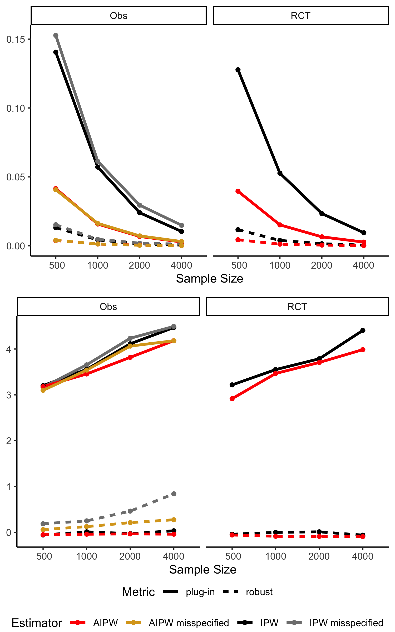
Figure 1: Estimation Performance of Different Calibration Error Estimators. The top and bottom panels show results of mean squared error and standardized bias, respectively. The two sub-panels within each panel show results under observational study and randomized trial settings, respectively. We consider two estimators (plug-in v.s. robust) and four scores with different types of model specification, where misspecified indicates the treatment model is misspecified; otherwise, both nuisance models are correctly specified. Overall, using the robust estimator with AIPW scores resulted in the best calibration error estimates.

The plug-in estimator showed an increasing trend between standardized bias and sample size, which may be explained by the relatively large bias shown in Table 1. In contrast, the robust estimator presented slightly decreasing trends under the RCT setting and nearly flat trends under the observational study setting. The increasing trend of the robust IPW misspecified estimator may be due to using incorrect propensity scores. Under this situation, the estimation errors from the Monte Carlo simulation can be dominating and further induce counterintuitive results.

The Obs panels in Figure 1 also show the impact of model misspecification on estimation performance. We see that the estimators using IPW scores produced a higher MSE and standardized bias when the treatment model is misspecified. In contrast, the incorrect propensity scores only slightly influenced AIPW estimators in terms of minor increase on the standardized bias and almost no change on the MSE.

Table 1 shows the performance of both estimators under three levels of miscalibration on four evaluation metrics. When both nuisance parameters are correctly estimated in the AIPW scores, the robust estimator yielded smaller biases than the plug-in estimator across all scenarios with comparable stability. Similar comparison results for IPW scores can be found in the Supplemental Materials.

Table 1: Performance of the Calibration Error Estimators under Observational Study Settings. The calibration function is estimated using an AIPW estimator with correctly modeled nuisance parameters. Under this setup, the robust estimator (bottom half of the table) outperformed the plug-in estimator (top half of the table) across all scenarios.

$\mathbf{\alpha}$	N	Bias	S.E.	S.bias	MSE
Plug-in estimator
0	500	0.2234	0.0644	3.4708	0.0541
	1000	0.1329	0.0358	3.7113	0.0189
	2000	0.0852	0.0189	4.5133	0.0076
	4000	0.0531	0.0114	4.6709	0.0029
0.15	500	0.2201	0.0655	3.3582	0.0527
	1000	0.1313	0.0388	3.3831	0.0188
	2000	0.0839	0.0207	4.0458	0.0075
	4000	0.0521	0.0130	3.9954	0.0029
0.3	500	0.2171	0.0733	2.9606	0.0525
	1000	0.1300	0.0463	2.8068	0.0191
	2000	0.0825	0.0266	3.1023	0.0075
	4000	0.0511	0.0173	2.9518	0.0029
Robust estimator
0	500	-0.0094	0.0658	-0.1436	0.0044
	1000	-0.0065	0.0359	-0.1809	0.0013
	2000	-0.0020	0.0193	-0.1062	0.0004
	4000	-0.0014	0.0116	-0.1230	0.0001
0.15	500	-0.0103	0.0675	-0.1522	0.0047
	1000	-0.0066	0.0391	-0.1681	0.0016
	2000	-0.0025	0.0213	-0.1159	0.0005
	4000	-0.0019	0.0132	-0.1430	0.0002
0.3	500	-0.0113	0.0752	-0.1507	0.0058
	1000	-0.0067	0.0466	-0.1446	0.0022
	2000	-0.0032	0.0271	-0.1188	0.0007
	4000	-0.0024	0.0174	-0.1375	0.0003

Table 2 shows the estimator performance under observational studies with high-dimensional covariates, in which the dimension of additional predictors (besides $X_{0}$ and $X_{1}$) varies from 50 to 400, and the miscalibration level is 0.15. We see both accuracy and efficiency dropped as the number of covariates $P$ goes up, but, overall, the robust estimator performed not much worse than in low dimension situations (Table 1). High-dimensional results for other estimators, study settings, and simulation scenarios are included in the Supplemental Materials.

To summarize, the AIPW-based robust ECETH estimator should be used in general for evaluating the calibration error in CATE estimates regardless of the study type and the dimension of covariates.

Table 2: Performance of the robust ECETH estimator under the high-dimensional settings. Assuming an observational study setting with a miscalibration level $\alpha$ of 0.15. An robust estimator with AIPW scores is used where both nuisance parameters are correctly modeled. The robust estimator performed roughly as well as in low dimension situations ($P=2$).

N	P	Bias	S.E.	S.bias	MSE
500	50	0.0053	0.0702	0.0759	0.0050
1000	50	0.0001	0.0366	0.0037	0.0013
	100	0.0060	0.0412	0.1454	0.0017
2000	50	0.0017	0.0228	0.0738	0.0005
	100	0.0044	0.0232	0.1919	0.0006
	200	0.0073	0.0257	0.2854	0.0007
4000	50	0.0008	0.0134	0.0616	0.0002
	100	0.0035	0.0136	0.2569	0.0002
	200	0.0070	0.0150	0.4639	0.0003
	400	0.0102	0.0166	0.6134	0.0004

4 Data Application

In this section, we use the proposed HTE calibration metric to evaluate two CATE models in an applied setting. The CRITEO-UPLIFT1 is a large-scale trial where a portion of users are randomly prevented from being targeted by advertising. Diemert et al. (2018) compared the performance of two uplift prediction models on this data set and showed that there exists treatment effect heterogeneity among users. CRITEO-UPLIFT1 data set contains the information of over 25M users on treatment, visit and conversion labels, and 12 features. The feature names are masked due to privacy concerns while preserving their ability of prediction. The visit and conversion labels are binary, and positive labels indicate that the user visited/converted on the advertiser website during the test period.

4.1 Analysis Procedures

We randomly sampled 640,000 users from the full CRITEO-UPLIFT1 data set and randomly selected half of the samples as the training set and the other half as the testing set. We derived two HTE models to estimate the user-level treatment effects, which are defined as the risk difference in conversion rate between users who are prevented and not prevented from being advertised. First, we apply the causal forest method in which tree splits are selected to maximize the heterogeneity in treatment effects between two daughter nodes (Athey et al., 2019). We fit a causal forest model with 500 trees, allowing all 12 variables to be randomly selected and tried at each split, and requiring 5000 minimal number of observations in each tree leaf. The second approach we applied is an S-learner of random forest. Specifically, we used all 12 features and the treatment variable to train a single model. Then, we made predictions on the “counterfactual” testing sets where the treatment value is 1 and 0 for all subjects separately. The HTEs are then computed as the difference between the estimated counterfactual outcomes. Both implementations are carried out using the R package grf. Causal forest directly estimates treatment effect heterogeneity and has been shown outperforming other conditional mean modeling approaches such as S-learner. Thus, we expect the causal forest to have a smaller calibration error than the S-learner model.

To evaluate the $\ell_{2}$-ECETH, we used the top-performing robust estimator $\widehat{\theta}_{\mathrm{robust}}$, with the calibration function estimated using the AIPW score in 10 bins. We computed the 95% confidence interval (CI) via bootstrapping (1000 bootstrap resamples), in which the 2.5% and 97.5% percentiles are the lower and upper bounds, respectively. Because the ECETH must be non-negative, but the unbiased estimates and confidence intervals need not be, we truncate any negative values at $0$.

4.2 Analysis Results

The average treatment effect (ATE) in our study sample is $1.2\times{10^{-3}}$ (95% CI: $9\times{10^{-4}}$, $1.4\times{10^{-3}}$), which is estimated using the same AIPW score that applied in the ECETH estimator. The ATE estimated by causal forest and S-learner over the test data are $1.1\times{10^{-3}}$ and $1.5\times{10^{-5}}$, respectively. Table 3 shows that the causal forest and the S-learner random forest resulted in at most root-$\ell_{2}$-ECETH of $\sqrt{8.9\times{10^{-7}}}=9\times{10^{-4}}$ and $\sqrt{6.8\times{10^{-6}}}=2.6\times{10^{-3}}$, respectively. In addition, Figure 2 shows that causal forest estimated CATE with large variability, but S-learner did not show much ability of estimating the heterogeneity in treatment effects. This is consistent with the result that causal forest model yielded a significantly smaller calibration error than the S-learner random forest model (Table 3).

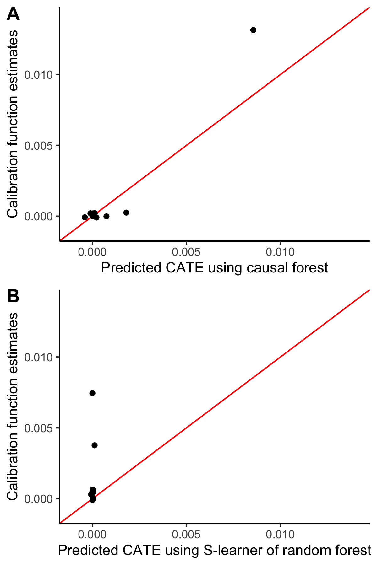
Figure 2: Calibration Plot between Predicted and Observed CATEs in CRITEO-UPLIFT1. Ten bins are used for computing the calibration function. The red line at 45 degrees indicates perfect calibration. The CATE estimates from causal forest are better calibrated than those from the S-learner of random forest.

Table 3: Calibration Errors of the CATE Models Derived Using CRITEO-UPLIFT Data.

HTE Model	Estimate	95% CI
Causal forest	0	(0, $8.9\times{10^{-7}}$)
Random forest	$4.2\times{10^{-6}}$	($2.1\times{10^{-6}}$, $6.8\times{10^{-6}}$)

5 Discussion

We propose a general calibration metric for evaluating heterogeneous treatment effects on continuous, binary, or survival outcomes. Our metric can be applied to both randomized trials or observational studies with high-dimensional covariates. Given a large amount of interest in HTE estimation and many proposals of novel statistical methods, it is crucial to compare available approaches and choose the top-performing one for deployment at clinical sites. Our metric serves exactly this purpose by providing a formal way to estimate the calibration error in HTE estimates. The correct identification of an accurate and efficient HTE model can support better treatment decision making, further achieving ultimate population health outcomes.

There are two potential limitations to our proposed method. In observational studies, the unbiased estimation of the calibration function can only be achieved when there are no unmeasured confounders. Otherwise, the estimated calibration error may be inaccurate. Also, the score are constructed using IPW based estimators that may be unstable with extreme weights, e.g., when the group sizes under treatment arms are very unbalanced or most of the subjects are censored before the time of interest.

As the key to calibration error estimation is to construct unbiased scores for CATE, one may also consider using innovative machine learning methods. For example, with a time-to-event outcome, one could apply the causal survival forest Cui et al. (2021) to provide a nonparametric estimation of the calibration functions in terms of the difference in (restricted) mean survival times. Moreover, our metric focuses on evaluating HTE estimates on the absolute risk difference scale, so a natural extension is to define the calibration function on the relative scale, which enables the assessment of HTE estimates such as relative risks or hazard ratios.

6 Acknowledgement

This work was partially supported by R01 HL144555 from the National Heart, Lung, and Blood Institute (NHLBI).

 

Supplementary Material:
Calibration Error for Heterogeneous Treatment Effects

 

Appendix A PROOFS

A.1 Asymptotic Linearity

As mentioned in Section 2.1.1, the cross-fitting estimator is the sum of $J$ separate estimators constructed using a sample splitting procedure. To show that this is asymptotically linear, we show that each of the $J$ estimators is asymptotically linear, which implies the result. With an abuse of notation, we will assume that there are $n$ observations in each partition, the first, containing observations $i=1,\dots,n$ denoted by $D_{1}$, and the rest are from a second partition $D_{2}$.

Theorem 1.

Let $\gamma_{\widehat{\tau}}(\delta)$ be $L$-Lipschitz, and consider the robust estimator

$$\widehat{\theta}_{\mathrm{robust}}=\frac{1}{n}\sum_{i=1}^{n}(\widehat{\Gamma}_{i}-\Delta_{i})(\widehat{\gamma}_{-i}(\Delta_{i})-\Delta_{i}),$$

where $\widehat{\Gamma}_{i}$ satisfies $\widehat{\Gamma}_{i}=\Gamma_{i}^{\ast}+e_{i}$, with $\{\Gamma_{i}^{\ast}\}_{i=1}^{n}$ i.i.d. and ${\rm Var}(\Gamma_{i}^{\ast}\mid\Delta_{i})<C$ almost everywhere, and $e_{i}$ satisfying the conditions given in Section 2.1.2: (a) $(X_{i},\Delta_{i},Y_{i},W_{i},e_{i})_{i=1}^{n}$ are independent given $D_{2}$, and (b) $\sqrt{n}\mathbb{E}[(\Gamma_{j}^{\ast}+e_{j}+\Delta_{j})e_{i}|D_{2}]=o_{P}(1)$ and $\mathbb{E}[e_{i}^{2}|D_{2}]=o_{P}(1)$. If $\Delta_{i}$ is bounded on $[-B,B]$ and has a density $0<1/C\leq p_{\Delta}(\delta)\leq C<\infty$, and the number of bins $K$ for fitting $\widehat{\gamma}(\cdot)$ is chosen so that $\sqrt{n}/K\to 0$ and $K/n\to 0$, then

$$\sqrt{n}(\widehat{\theta}_{\mathrm{robust}}-\theta)=\frac{1}{\sqrt{n}}\sum_{i=1}^{n}\psi(X_{i},\Delta_{i},Y_{i},W_{i})+o_{P}(1),$$

for some fixed mean-zero influence function $\psi(\cdot)$, $\mathbb{E}[\psi(X_{i},\Delta_{i},Y_{i},W_{i})]=0$ with bounded variance, $\mathbb{E}[\psi^{2}(X_{i},\Delta_{i},Y_{i},W_{i})]<\infty$.

Proof    First, we will show the result for when $e_{1}=\dots=e_{n}=0$, so that there is no score approximation error. This comes up when working with a randomized trial and using the IPW score, and also serves as the first step in showing the full result.

In this, we will abuse notation and write $\widehat{\gamma}(\Delta_{i})$ in place of $\widehat{\gamma}_{\widehat{\tau},-i}(\Delta_{i})$, implicitly assuming that the estimator leaves out the observation associated with it’s argument.

Step 1: No score approximation error

Consider the following decomposition of $\sqrt{n}(\widehat{\theta}_{\mathrm{robust}}-\theta)$ into two terms,

$$\frac{1}{\sqrt{n}}\sum_{i=1}^{n}(\Gamma_{i}^{\ast}-\Delta_{i})(\widehat{\gamma}(\Delta_{i})-\Delta_{i})-\theta=\underbrace{\frac{1}{\sqrt{n}}\sum_{i=1}^{n}(\Gamma_{i}^{\ast}-\Delta_{i})(\widehat{\gamma}(\Delta_{i})-\gamma(\Delta_{i}))}_{(\star)}+\underbrace{\frac{1}{\sqrt{n}}\sum_{i=1}^{n}(\Gamma_{i}^{\ast}-\Delta_{i})(\gamma(\Delta_{i})-\Delta_{i})-\theta}_{(\star\star)}.$$

Term $(\star\star)$ is already in the form of an unbiased average of mean zero random variables, so we will set it aside for now. Term $(\ast)$ we will further decompose into such a component, as well as some lower-order terms. Recall that $\widehat{\gamma}_{\widehat{\tau},-i}(\delta)$ is a binned average, written in (2.2), for $k$ such that $\delta\in R_{k}$. With this in mind, we can expand $(\star)$ as follows:

$$(\star) =\frac{1}{\sqrt{n}}\sum_{i=1}^{n}(\gamma(\Delta_{i})-\Delta_{i})(\widehat{\gamma}(\Delta_{i})-\gamma(\Delta_{i}))+\frac{1}{\sqrt{n}}\sum_{i=1}^{n}(\Gamma_{i}^{\ast}-\gamma(\Delta_{i}))(\widehat{\gamma}(\Delta_{i})-\gamma(\Delta_{i}))$$

$$=\underbrace{\frac{1}{\sqrt{n}}\sum_{i=1}^{n}(\gamma(\Delta_{i})-\Delta_{i})\left(\frac{1}{|I_{k}|-1}\sum_{\begin{subarray}{c}j\in I_{k}\\ j\not=i\end{subarray}}\Gamma_{i}^{\ast}-\gamma(\Delta_{i})\right)}_{(3\star)}+\underbrace{\frac{1}{\sqrt{n}}\sum_{i=1}^{n}(\Gamma_{i}^{\ast}-\gamma(\Delta_{i}))(\widehat{\gamma}(\Delta_{i})-\gamma(\Delta_{i}))}_{(4\star)}$$

Notice that the $j$-th term in a given set $I_{k}$ appears in $(3\star)$ for all other $i\in I_{k}$, so carefully re-ordering the summation gives

$$(3\star) =\frac{1}{\sqrt{n}}\sum_{i=1}^{n}\Gamma_{i}^{\ast}\left(\frac{1}{|I_{k}|}\sum_{\begin{subarray}{c}j\in I_{k}\\ i\not=j\end{subarray}}(\gamma(\Delta_{j})-\Delta_{j})\right)-\frac{1}{\sqrt{n}}\sum_{i=1}^{n}\gamma(\Delta_{i})(\gamma(\Delta_{i})-\Delta_{i})$$

Adding and subtracting the following term separates this into an error term $$(5\star) (6\star)$$ and influence function component :

$$=\frac{1}{\sqrt{n}}\sum_{i=1}^{n}\Gamma_{i}^{\ast}\left(\frac{1}{|I_{k}|}\sum_{\begin{subarray}{c}j\in I_{k}\\ i\not=j\end{subarray}}(\gamma(\Delta_{j})-\Delta_{j})\right)-\frac{1}{\sqrt{n}}\sum_{i=1}^{n}\gamma(\Delta_{i})(\gamma(\Delta_{i})-\Delta_{i})$$

$$~{}\quad~{}\quad~{}\quad~{}\quad-\frac{1}{\sqrt{n}}\sum_{i=1}^{n}\Gamma_{i}^{\ast}(\gamma(\Delta_{i})-\Delta_{i})+\frac{1}{\sqrt{n}}\sum_{i=1}^{n}\Gamma_{i}^{\ast}(\gamma(\Delta_{i})-\Delta_{i})$$

$$=\underbrace{\frac{1}{\sqrt{n}}\sum_{i=1}^{n}\Gamma_{i}^{\ast}\left(\frac{1}{|I_{k}|}\sum_{\begin{subarray}{c}j\in I_{k}\\ i\not=j\end{subarray}}(\gamma(\Delta_{j})-\Delta_{j})-\gamma(\Delta_{i})+\Delta_{i}\right)}_{(5\star)}+\underbrace{\frac{1}{\sqrt{n}}\sum_{i=1}^{n}(\Gamma_{i}^{\ast}-\gamma(\Delta_{i}))(\gamma(\Delta_{i})-\Delta_{i})}_{(6\star)}.$$

Showing that $(4\ast)$ and $(5\ast)$ converge in probability to $0$ will imply that $\sqrt{n}(\widehat{\theta}_{\mathrm{robust}}-\theta)=(\star\star)+(6\star)+o_{P}(1)$, completing the result.

Starting with $(4\ast)$, notice that this term is mean zero, by applying the tower rule conditioning on $\Delta_{i}$, observing that $\mathbb{E}[\Gamma_{i}^{\ast}-\gamma(\Delta_{i})\mid\Delta_{i}]=0$, and recalling that $\widehat{\gamma}(\Delta_{i})$ is implicitly an estimator leaving out observation $i$, so it is independent of $\Gamma_{i}^{\ast}$ conditional on $\Delta_{i}$. Therefore, Chebyshev’s inequality implies that for any $\epsilon>0$

$$P\left(\left|\frac{1}{\sqrt{n}}\sum_{i=1}^{n}(\Gamma_{i}^{\ast}-\gamma(\Delta_{i}))(\widehat{\gamma}(\Delta_{i})-\gamma(\Delta_{i}))\right|>\epsilon\right)\leq\frac{{\rm Var}\left(\frac{1}{\sqrt{n}}\sum_{i=1}^{n}(\Gamma_{i}^{\ast}-\gamma(\Delta_{i}))(\widehat{\gamma}(\Delta_{i})-\gamma(\Delta_{i}))\right)}{\epsilon^{2}}$$

Letting $\bar{\gamma}(\delta)=\mathbb{E}[\widehat{\gamma}(\delta)]=\mathbb{E}[\Gamma_{i}^{\ast}\mid\Delta_{i}\in R_{k}],$ for $k$ such that $\delta\in R_{k}$, notice that

$${\rm Var}\left(\frac{1}{\sqrt{n}}\sum_{i=1}^{n}(\Gamma_{i}^{\ast}-\gamma(\Delta_{i}))(\widehat{\gamma}(\Delta_{i})-\gamma(\Delta_{i}))\right) \leq 2{\rm Var}\left(\frac{1}{\sqrt{n}}\sum_{i=1}^{n}(\Gamma_{i}^{\ast}-\gamma(\Delta_{i}))(\bar{\gamma}(\Delta_{i})-\gamma(\Delta_{i}))\right)$$

$$~{}\quad~{}\quad+2{\rm Var}\left(\frac{1}{\sqrt{n}}\sum_{i=1}^{n}(\Gamma_{i}^{\ast}-\gamma(\Delta_{i}))(\widehat{\gamma}(\Delta_{i})-\bar{\gamma}(\Delta_{i}))\right).$$

The first variance is bounded by $C\|\bar{\gamma}(\cdot)-\gamma(\cdot)\|_{2,P}^{2}$, where $\|\cdot\|_{2,P}^{2}$ is the mean integrated squared error (MISE) of the argument under measure $P$. Using standard results for the MISE of the binned estimator (Chen, 2019), we know that $\|\bar{\gamma}(\cdot)-\gamma(\cdot)\|_{2,P}^{2}=O(1/K^{2}+K/n)$. The second is more subtle, but can be shown using results from $U$-statistics. Re-writing the sum over $i=1,\dots,n$ as $\sum_{k=1}^{K}\sum_{i\in I_{k}}$, notice that within each $k$, we have (nearly) a $U$-statistic with $|I_{k}|$ observations,

$$\frac{1}{\sqrt{n}}\sum_{i=1}^{n}(\Gamma_{i}^{\ast}-\gamma(\Delta_{i}))(\widehat{\gamma}(\Delta_{i})-\bar{\gamma}(\Delta_{i}))=\frac{1}{\sqrt{n}}\sum_{k=1}^{K}|I_{k}|\frac{1}{(|I_{k}|-1)|I_{k}|}\sum_{i\in I_{k}}\sum_{\begin{subarray}{c}j\in I_{k}\\ j\not=i\end{subarray}}(\Gamma_{i}^{\ast}-\gamma(\Delta_{i}))(\Gamma_{j}^{\ast}-\mathbb{E}[\Gamma_{i}^{\ast}\mid\Delta_{i}\in R_{k}]).$$

Using standard results for $U$-statistics (Doksum, 2008), the term $\frac{1}{(|I_{k}|-1)|I_{k}|}\sum_{i\in I_{k}}\sum_{\begin{subarray}{c}j\in I_{k}\\ j\not=i\end{subarray}}(\Gamma_{i}^{\ast}-\gamma(\Delta_{i}))(\Gamma_{j}^{\ast}-\mathbb{E}[\Gamma_{i}^{\ast}\mid\Delta_{i}\in R_{k}])$ has variance bounded by $C/((|I_{k}|-1)|I_{k}|)$. Each of these $K$ terms are independent, and so overall, we have

$${\rm Var}\left(\frac{1}{\sqrt{n}}\sum_{k=1}^{K}|I_{k}|\frac{1}{(|I_{k}|-1)|I_{k}|}\sum_{i\in I_{k}}\sum_{\begin{subarray}{c}j\in I_{k}\\ j\not=i\end{subarray}}(\Gamma_{i}^{\ast}-\gamma(\Delta_{i}))(\Gamma_{j}^{\ast}-\mathbb{E}[\Gamma_{i}^{\ast}\mid\Delta_{i}\in R_{k}])\right)\leq\frac{K}{n}C.$$

By assumption, $K/n\to 0$. Therefore, altogether, we have

$$P\left(\left|\frac{1}{\sqrt{n}}\sum_{i=1}^{n}(\Gamma_{i}^{\ast}-\gamma(\Delta_{i}))(\widehat{\gamma}(\Delta_{i})-\gamma(\Delta_{i}))\right|>\epsilon\right)\leq\frac{CK/n+C(1/K^{2}+K/n)}{\epsilon^{2}}\to 0.$$

Showing that $(5\star)\stackrel{{\scriptstyle p}}{{\rightarrow}}0$ has 3 parts. Two of them are like what we did for $(4\star)$. Splitting this term into parts,

$$(5\star) =\frac{1}{\sqrt{n}}\sum_{i=1}^{n}(\Gamma_{i}^{\ast}-\gamma(\Delta_{i})\left(\frac{1}{|I_{k}|}\sum_{\begin{subarray}{c}j\in I_{k}\\ i\not=j\end{subarray}}(\gamma(\Delta_{j})-\Delta_{j})-\gamma(\Delta_{i})+\Delta_{i}\right)$$

$$~{}\quad~{}\quad+\frac{1}{\sqrt{n}}\sum_{i=1}^{n}\gamma(\Delta_{i})\left(\frac{1}{|I_{k}|}\sum_{\begin{subarray}{c}j\in I_{k}\\ i\not=j\end{subarray}}(\gamma(\Delta_{j})-\Delta_{j})-\gamma(\Delta_{i})+\Delta_{i}\right).$$

The first term is mean $0$ and variance bounded by $C\|\widehat{\gamma}(\Delta_{i})-\gamma(\Delta_{i})\|_{2,P}^{2}\to 0$, so by Chebyshev’s inequality, it is asymptotically negligible. For the second term, we must decompose it again into a bias component and a variance component.

$$\frac{1}{\sqrt{n}}\sum_{i=1}^{n}\gamma(\Delta_{i})\left(\frac{1}{|I_{k}|}\sum_{\begin{subarray}{c}j\in I_{k}\\ i\not=j\end{subarray}}(\gamma(\Delta_{j})-\Delta_{j})-\gamma(\Delta_{i})+\Delta_{i}\right)$$

$$=\frac{1}{\sqrt{n}}\sum_{i=1}^{n}\gamma(\Delta_{i})\left(\mathbb{E}[\gamma(\Delta)-\Delta\mid\Delta\in R_{k}]-\gamma(\Delta_{i})+\Delta_{i}\right)$$

$$~{}\quad~{}+\frac{1}{\sqrt{n}}\sum_{k=1}^{K}\sum_{i\in I_{k}}\gamma(\Delta_{i})\left(\frac{1}{|I_{k}|}\sum_{\begin{subarray}{c}j\in I_{k}\\ i\not=j\end{subarray}}(\gamma(\Delta_{j})-\Delta_{j})-\mathbb{E}[\gamma(\Delta)-\Delta\mid\Delta\in R_{k}]\right)$$

By Cauchy-Schwarz,

$$\left|\frac{1}{\sqrt{n}}\sum_{i=1}^{n}\gamma(\Delta_{i})\left(\mathbb{E}[\gamma(\Delta)-\Delta\mid\Delta\in R_{k}]-\gamma(\Delta_{i})+\Delta_{i}\right)\right|$$

$$\leq\sqrt{\left(\frac{1}{n}\sum_{i=1}^{n}\gamma^{2}(\Delta_{i})\right)\left(\frac{n}{n}\sum_{k=1}^{K}\sum_{i\in I_{k}}(\mathbb{E}[\gamma(\Delta)-\Delta\mid\Delta\in R_{k}]-\gamma(\Delta_{i})+\Delta_{i})^{2}\right)}$$

and because $$\delta\mapsto\gamma(\delta)+\delta L+1$$ is -Lipschitz,

$$\leq\sqrt{\left(\frac{1}{n}\sum_{i=1}^{n}\gamma^{2}(\Delta_{i})\right)\left(\frac{n}{n}\sum_{k=1}^{K}\sum_{i\in I_{k}}|R_{k}|^{2}(L+1)^{2}\right)}.$$

Noting that by the construction of the binning estimator, and the fact that the distribution of $\Delta_{i}$ was assumed to be equivalent (up to a scale factor) to the uniform distribution, $\exists c>0$ and a random variable $S$ such that $S\sim\mathrm{Beta}(n/K,n-n/K+1)$ and $cS<|R_{k}|<S/c$, almost surely. Therefore, $n\mathbb{E}[|R_{k}|^{2}]\leq n/(cK^{2})\to 0$ (because we assumed $n/K^{2}\to 0$), and so by Markov’s inequality, this term is $o_{P}(1)$.

Finally, using a similar $U$-statistic argument as above, the final remaining term is unbiased and has variance bounded by $CK/n$, so by Chebyshev’s inequality it is asymptotically negligible.

Step 2: Addressing score approximation error

The approximation error term is

$$\frac{1}{\sqrt{n}}\sum_{i=1}^{n}e_{i}\left(\frac{1}{|I_{k}|-1}\sum_{\begin{subarray}{c}j\in I_{k}\\ i\not=j\end{subarray}}\Gamma_{j}^{\ast}+e_{j}-\Delta_{i}\right)+\frac{1}{\sqrt{n}}\sum_{i=1}^{n}\left(\Gamma_{i}^{\ast}-\Delta_{i}\right)\left(\frac{1}{|I_{k}|-1}\sum_{\begin{subarray}{c}j\in I_{k}\\ i\not=j\end{subarray}}e_{j}\right).$$

Noting that due to the symmetry of the binning estimator, these two terms are substantially equivalent, we show here only that the first term is asymptotically negligible.

To this end, expand

$$\frac{1}{\sqrt{n}}\sum_{i=1}^{n}e_{i}\left(\frac{1}{|I_{k}|-1}\sum_{\begin{subarray}{c}j\in I_{k}\\ i\not=j\end{subarray}}\Gamma_{j}^{\ast}+e_{j}-\Delta_{i}\right) =\frac{1}{\sqrt{n}}\sum_{i=1}^{n}e_{i}\left(\frac{1}{|I_{k}|-1}\sum_{\begin{subarray}{c}j\in I_{k}\\ i\not=j\end{subarray}}\Gamma_{j}^{\ast}-\mathbb{E}[\Gamma_{j}^{\ast}\mid\Delta_{j}\in R_{k}]\right)$$

$$~{}\quad~{}+\frac{1}{\sqrt{n}}\sum_{i=1}^{n}e_{i}\left(\mathbb{E}[\Gamma_{j}^{\ast}\mid\Delta_{j}\in R_{k}]-\Delta_{i}\right)$$

$$~{}\quad~{}+\frac{1}{\sqrt{n}}\sum_{i=1}^{n}\frac{1}{|I_{k}|-1}\sum_{\begin{subarray}{c}j\in I_{k}\\ i\not=j\end{subarray}}e_{i}e_{j}$$

The first term is mean 0, and has variance bounded by $\mathbb{E}[C/n\sum_{i=1}^{n}e_{i}^{2}/|I_{k}|\mid D_{2}]\stackrel{{\scriptstyle p}}{{\rightarrow}}0$, so by Chebyshev’s inequality it is lower order. The bias of the second term is lower order, because

$$\mathbb{E}\left[\frac{\sqrt{n}}{n}\sum_{i=1}^{n}e_{i}(\mathbb{E}[\Gamma_{i}^{\ast}\mid\Delta_{i}\in R_{k}]-\Delta_{i})\mid D_{2}\right]\leq|\sqrt{n}\mathbb{E}\left[e_{i}(\tau(X_{i})-\Delta_{i})\mid D_{2}\right]|+|\sqrt{n}\mathbb{E}\left[e_{i}2L|R_{K}|\mid D_{2}\right]|\stackrel{{\scriptstyle p}}{{\rightarrow}}0$$

by assumption. The variance is lower order because conditional on $D_{2}$, the errors are independent, so

$$\mathbb{E}\left[\left(\frac{1}{\sqrt{n}}\sum_{i=1}^{n}e_{i}(\mathbb{E}[\Gamma_{i}^{\ast}\mid\Delta_{i}\in R_{k}]-\Delta_{i})\right)^{2}\right] =\frac{1}{n}\sum_{i=1}^{n}\mathbb{E}\left[e_{i}^{2}(\mathbb{E}[\Gamma_{i}^{\ast}\mid\Delta_{i}\in R_{k}]-\Delta_{i})^{2}\mid D_{2}\right]$$

$$~{}\quad~{}+\frac{1}{n}\sum_{i\not=j}\mathbb{E}\left[e_{i}(\mathbb{E}[\Gamma_{i}^{\ast}\mid\Delta_{i}\in R_{k}]-\Delta_{i})\mid D_{2}\right]\cdot$$

$$~{}\quad~{}\quad~{}\quad~{}\quad~{}\quad~{}\quad~{}\quad~{}\quad\mathbb{E}\left[e_{i}(\mathbb{E}[\Gamma_{i}^{\ast}\mid\Delta_{i}\in R_{k}]-\Delta_{i})\mid D_{2}\right]$$

$$\leq o_{P}(1)+\frac{1}{n^{2}}\sum_{i\not=j}\sqrt{n}\mathbb{E}\left[e_{i}(\mathbb{E}[\Gamma_{i}^{\ast}\mid\Delta_{i}\in R_{k}]-\Delta_{i})\mid D_{2}\right]\cdot$$

$$~{}\quad~{}\quad~{}\quad~{}\quad~{}\quad~{}\quad~{}\quad~{}\quad\sqrt{n}\mathbb{E}\left[e_{i}(\mathbb{E}[\Gamma_{i}^{\ast}\mid\Delta_{i}\in R_{k}]-\Delta_{i})\mid D_{2}\right]$$

$$\leq o_{P}(1)+\left(\frac{1}{n}\sum_{i=1}^{n}\sqrt{n}\mathbb{E}\left[e_{i}(\mathbb{E}[\Gamma_{i}^{\ast}\mid\Delta_{i}\in R_{k}]-\Delta_{i})\mid D_{2}\right]\right)^{2}$$

$$=o_{P}(1),$$

as before. The final term follows from yet another application of Chebyshev’s inequality, noticing that only the terms within one bin have nonzero cross terms, and applying the same analysis as above within each bin. ∎

A.2 APPROXIMATION ERROR

Here, we describe how to meet the needed approximation error terms of the asymptotic linearity result above using cross-fitting and the AIPW estimator. When performing cross-fitting, we split the data into two independent and identically distributed pieces, $D_{1}$ and $D_{2}$, and use $D_{2}$ to fit the propensity score estimator $\widehat{\pi}(\cdot)$ and outcome model $\widehat{\mu}(\cdot,\cdot)$. Then, we apply the estimated nuisance parameters to the estimator the $D_{1}$. This can be repeated in reverse to use the full sample size for the estimator, but still maintain the independence of the nuisance components.

With this in mind, we will check the approximation error conditions conditional on $D_{2}$, so that we can treat $\widehat{\pi}(\cdot)$ and $\widehat{\mu}(\cdot,\cdot)$ as fixed, and then assume that when trained on $D_{2}$, they achieve certain necessary estimation error properties with high probability.

The AIPW estimation error can be written as follows:

$$\widehat{\mu}(X_{i},1)-\mu(X_{i},1)-\widehat{\mu}(X_{i},0)+\mu(X_{i},0)+\frac{W_{i}-\widehat{\pi}(X_{i})}{\widehat{\pi}(X_{i})(1-\widehat{\pi}(X_{i}))}(Y_{i}-\widehat{\mu}(X_{i},W_{i}))-\frac{W_{i}-\pi(X_{i})}{\pi(X_{i})(1-\pi(X_{i}))}(Y_{i}-{\mu}(X_{i},W_{i})).$$

We will focus only on the term

$$e_{i}:=\widehat{\mu}(X_{i},1)-\mu(X_{i},1)+\frac{W_{i}}{\widehat{\pi}(X_{i})}(Y_{i}-\widehat{\mu}(X_{i},1))-\frac{W_{i}}{{\pi}(X_{i})}(Y_{i}-{\mu}(X_{i},1)),$$

as the term for $\mathbb{E}[Y(0)\mid X=x]$ is identical. Notice that

$$\mathbb{E}[e_{i}\mid X_{i}]=\widehat{\mu}(X_{i},1)-\mu(X_{i},1)+\frac{\pi(X_{i})}{\widehat{\pi}(X_{i})}(\mu(X_{i},1)-\widehat{\mu}(X_{i},1))=\left(\frac{\widehat{\pi}(X_{i})-\pi(X_{i})}{\widehat{\pi}(X_{i})}\right)(\mu(X_{i},1)-\widehat{\mu}(X_{i},1)).$$

As long as $0<\epsilon\leq\widehat{\pi}(X_{i})\leq 1-\epsilon$, then

$$\sqrt{n}\mathbb{E}[e_{i}(\Gamma_{i}^{\ast}+\Delta_{i})]\leq\frac{C}{\epsilon}\sqrt{n}\|\widehat{\pi}(\cdot)-\pi(\cdot)\|_{2q,P}\|(\mu(\cdot,1)-\widehat{\mu}(\cdot,1)\|_{2p,P},$$

where $1/q+1/p=1$. This can be achieved as long as $\widehat{\pi}$ and $\widehat{\mu}$ can be estimated at $n^{-1/4}$ rates, as is standard in semiparametric statistics (Chernozhukov et al., 2018a).

Similarly,

$$\mathbb{E}[e_{i}^{2}\mid X_{i}]\leq 2(\widehat{\mu}(X_{i},1)-\mu(X_{i},1))^{2}+4W_{i}\left(\left(\frac{1}{\widehat{\pi}(X_{i})}-\frac{1}{\pi(X_{i})}\right)^{2}Y_{i}^{2}+\left(\frac{\mu(X_{i},1)}{\pi(X_{i})}-\frac{\widehat{\mu}(X_{i},1)}{\widehat{\pi}(X_{i})}\right)^{2}\right),$$

which if $\|\widehat{\mu}(\cdot,1)-\mu(\cdot,1)\|_{2}\to 0$ and $\|\widehat{\pi}(\cdot)-\pi(\cdot)\|_{2}\to 0$, then $E[e_{i}^{2}]=o(1)$.

Appendix B ADDITIONAL EXPERIMENTS

Table 4: Performance of the Calibration Error Estimators under Observational Study Settings. The calibration function is estimated using an AIPW score with incorrectly specified propensity scores. Under this setup, the robust estimator (bottom half of the table) outperformed the plug-in estimator (top half of the table) across all scenarios.

$\mathbf{\alpha}$	N	Bias	S.E.	S.bias	MSE
Plug-in estimator
0	500	0.2121	0.0609	3.4843	0.0487
	1000	0.1288	0.0348	3.6988	0.0178
	2000	0.0831	0.0191	4.3638	0.0073
	4000	0.0525	0.0103	5.0789	0.0029
0.15	500	0.2182	0.0676	3.2290	0.0522
	1000	0.1330	0.0364	3.6567	0.0190
	2000	0.0847	0.0215	3.9423	0.0076
	4000	0.0537	0.0130	4.1244	0.0031
0.15	500	0.2131	0.0709	3.0058	0.0505
	1000	0.1304	0.0425	3.0678	0.0188
	2000	0.0836	0.0271	3.0893	0.0077
	4000	0.0541	0.0170	3.1857	0.0032
Robust estimator
0	500	-0.0086	0.0624	-0.1374	0.0040
	1000	-0.0058	0.0355	-0.1647	0.0013
	2000	-0.0016	0.0196	-0.0806	0.0004
	4000	-0.0006	0.0105	-0.0550	0.0001
0.15	500	-0.0014	0.0693	-0.0208	0.0048
	1000	-0.0011	0.0373	-0.0293	0.0014
	2000	0.0004	0.0218	0.0164	0.0005
	4000	0.0009	0.0132	0.0661	0.0002
0.3	500	-0.0053	0.0719	-0.0733	0.0052
	1000	-0.0031	0.0432	-0.0709	0.0019
	2000	-0.0003	0.0273	-0.0107	0.0007
	4000	0.0015	0.0171	0.0853	0.0003

Table 5: Performance of the Calibration Error Estimators under Observational Study Settings. The calibration function is estimated using an IPW score with correctly specified propensity scores. Under this setup, the robust estimator (bottom half of the table) outperformed the plug-in estimator (top half of the table) across all scenarios.

$\mathbf{\alpha}$	N	Bias	S.E.	S.bias	MSE
Plug-in estimator
0	500	0.3711	0.1135	3.2713	0.1506
	1000	0.2292	0.0631	3.6329	0.0565
	2000	0.1522	0.0344	4.4249	0.0243
	4000	0.1012	0.0202	5.0027	0.0106
0.15	500	0.3578	0.1118	3.2013	0.1405
	1000	0.2301	0.0647	3.5560	0.0571
	2000	0.1507	0.0366	4.1139	0.0240
	4000	0.0994	0.0223	4.4690	0.0104
0.3	500	0.3559	0.1252	2.8424	0.1423
	1000	0.2235	0.0696	3.2087	0.0548
	2000	0.1499	0.0433	3.4586	0.0243
	4000	0.0982	0.0277	3.5450	0.0104
Robust estimator
0	500	0.0011	0.1149	0.0091	0.0132
	1000	-0.0041	0.0639	-0.0634	0.0041
	2000	-0.0019	0.0349	-0.0548	0.0012
	4000	0.0009	0.0207	0.0419	0.0004
0.15	500	-0.0064	0.1147	-0.0559	0.0132
	1000	0.0008	0.0659	0.0127	0.0043
	2000	-0.0010	0.0373	-0.0259	0.0014
	4000	0.0008	0.0225	0.0354	0.0005
0.3	500	-0.0034	0.1280	-0.0269	0.0164
	1000	-0.0028	0.0711	-0.0399	0.0051
	2000	-0.0007	0.0439	-0.0160	0.0019
	4000	0.0004	0.0280	0.0136	0.0008

Table 6: Performance of the Calibration Error Estimators under Observational Study Settings. The calibration function is estimated using an IPW score with incorrectly specified propensity scores. Under this setup, the robust estimator (bottom half of the table) outperformed the plug-in estimator (top half of the table) across all scenarios.

$\mathbf{\alpha}$	N	Bias	S.E.	S.bias	MSE
Plug-in estimator
0	500	0.3585	0.1078	3.3251	0.1401
	1000	0.2367	0.0615	3.8484	0.0598
	2000	0.1636	0.0383	4.2694	0.0282
	4000	0.1121	0.0218	5.1388	0.0131
0.15	500	0.3726	0.1176	3.1674	0.1527
	1000	0.2388	0.0653	3.6550	0.0613
	2000	0.1672	0.0395	4.2346	0.0295
	4000	0.1191	0.0265	4.4927	0.0149
0.3	500	0.3563	0.1181	3.0172	0.1409
	1000	0.2451	0.0728	3.3673	0.0654
	2000	0.1680	0.0473	3.5550	0.0305
	4000	0.1178	0.0315	3.7434	0.0149
Robust estimator
0	500	0.0047	0.1099	0.0431	0.0121
	1000	0.0121	0.0624	0.1939	0.0040
	2000	0.0142	0.0390	0.3646	0.0017
	4000	0.0147	0.0219	0.6725	0.0007
0.15	500	0.0230	0.1214	0.1893	0.0153
	1000	0.0167	0.0662	0.2516	0.0047
	2000	0.0185	0.0398	0.4643	0.0019
	4000	0.0224	0.0266	0.8413	0.0012
0.3	500	0.0094	0.1200	0.0782	0.0145
	1000	0.0236	0.0737	0.3205	0.0060
	2000	0.0202	0.0478	0.4239	0.0027
	4000	0.0213	0.0315	0.6783	0.0014

Table 7: Performance of the Calibration Error Estimators under Randomized Trial Settings. The calibration function is estimated using an IPW score. Under this setup, the robust estimator (bottom half of the table) outperformed the plug-in estimator (top half of the table) across all scenarios.

$\mathbf{\alpha}$	N	Bias	S.E.	S.bias	MSE
Plug-in estimator
0	500	0.3458	0.1055	3.2765	0.1307
	1000	0.2217	0.0579	3.8268	0.0525
	2000	0.1486	0.0349	4.2592	0.0233
	4000	0.0981	0.0200	4.9073	0.0100
0.15	500	0.3413	0.1061	3.2177	0.1278
	1000	0.2210	0.0622	3.5512	0.0527
	2000	0.1479	0.0391	3.7870	0.0234
	4000	0.0948	0.0215	4.4060	0.0095
0.3	500	0.3414	0.1224	2.7889	0.1315
	1000	0.2201	0.0723	3.0440	0.0537
	2000	0.1431	0.0439	3.2613	0.0224
	4000	0.0940	0.0280	3.3554	0.0096
Robust estimator
0	500	-0.0039	0.1079	-0.0361	0.0117
	1000	-0.0020	0.0586	-0.0345	0.0034
	2000	-0.0004	0.0351	-0.0123	0.0012
	4000	0.0010	0.0201	0.0481	0.0004
0.15	500	-0.0043	0.1082	-0.0395	0.0117
	1000	0.0001	0.0626	0.0013	0.0039
	2000	0.0005	0.0393	0.0129	0.0015
	4000	-0.0013	0.0217	-0.0594	0.0005
0.3	500	0.0006	0.1238	0.0048	0.0153
	1000	0.0010	0.0725	0.0135	0.0053
	2000	-0.0026	0.0443	-0.0581	0.0020
	4000	-0.0013	0.0282	-0.0458	0.0008

Table 8: Performance of the Calibration Error Estimators under Randomized Trial Settings. The calibration function is estimated using an AIPW score. Under this setup, the robust estimator (bottom half of the table) outperformed the plug-in estimator (top half of the table) across all scenarios.

$\mathbf{\alpha}$	N	Bias	S.E.	S.bias	MSE
Plug-in estimator
0	500	0.2241	0.0724	3.0975	0.0555
	1000	0.1358	0.0387	3.5105	0.0199
	2000	0.0857	0.0205	4.1794	0.0078
	4000	0.0545	0.0113	4.8006	0.0031
0.15	500	0.2148	0.0683	3.1446	0.0508
	1000	0.1273	0.0377	3.3774	0.0176
	2000	0.0818	0.0207	3.9578	0.0071
	4000	0.0511	0.0129	3.9475	0.0028
0.3	500	0.2042	0.0775	2.6351	0.0477
	1000	0.1222	0.0438	2.7858	0.0168
	2000	0.0791	0.0274	2.8834	0.0070
	4000	0.0487	0.0181	2.6956	0.0027
Robust estimator
0	500	-0.0013	0.0729	-0.0175	0.0053
	1000	0.0005	0.0393	0.0121	0.0015
	2000	-0.0002	0.0207	-0.0098	0.0004
	4000	0.0003	0.0114	0.0242	0.0001
0.15	500	-0.0056	0.0700	-0.0798	0.0049
	1000	-0.0055	0.0384	-0.1434	0.0015
	2000	-0.0022	0.0208	-0.1039	0.0004
	4000	-0.0019	0.0130	-0.1466	0.0002
0.3	500	-0.0122	0.0785	-0.1550	0.0063
	1000	-0.0085	0.0442	-0.1914	0.0020
	2000	-0.0035	0.0277	-0.1263	0.0008
	4000	-0.0033	0.0181	-0.1843	0.0003

Table 9: Performance of the robust ECETH estimator under the high-dimensional settings. Assuming an observational study setting with three levels of miscalibration ($\alpha$). An AIPW score is used for the calibration function with correctly specified nuisance parameters. The robust estimator performed roughly as well as in low dimension situations ($P=2$).

			Robust estimator				Plug-in estimator
$\alpha$	N	P	Bias	S.E.	S.bias	MSE	Bias	S.E.	S.bias	MSE
0	500	50	0.0005	0.0704	0.0072	0.0050	0.2187	0.0694	3.1502	0.0526
	1000	50	0.0011	0.0364	0.0306	0.0013	0.1337	0.0358	3.7374	0.0191
		100	0.0030	0.0358	0.0833	0.0013	0.1390	0.0352	3.9494	0.0206
	2000	50	0.0003	0.0202	0.0169	0.0004	0.0859	0.0200	4.2894	0.0078
		100	0.0003	0.0212	0.0160	0.0004	0.0872	0.0207	4.2051	0.0080
		200	0.0035	0.0228	0.1516	0.0005	0.0982	0.0223	4.4078	0.0101
	4000	50	0.0000	0.0111	-0.0027	0.0001	0.0549	0.0110	4.9765	0.0031
		100	0.0009	0.0113	0.0833	0.0001	0.0563	0.0112	5.0356	0.0033
		200	0.0022	0.0130	0.1691	0.0002	0.0618	0.0128	4.8239	0.0040
		400	0.0043	0.0147	0.2931	0.0002	0.0713	0.0147	4.8649	0.0053
0.15	500	50	0.0053	0.0702	0.0759	0.0050	0.2205	0.0687	3.2085	0.0534
	1000	50	0.0001	0.0366	0.0037	0.0013	0.1312	0.0358	3.6634	0.0185
		100	0.0060	0.0412	0.1454	0.0017	0.1407	0.0407	3.4572	0.0214
	2000	50	0.0017	0.0228	0.0738	0.0005	0.0860	0.0224	3.8387	0.0079
		100	0.0044	0.0232	0.1919	0.0006	0.0902	0.0228	3.9506	0.0087
		200	0.0073	0.0257	0.2854	0.0007	0.1011	0.0254	3.9858	0.0109
	4000	50	0.0008	0.0134	0.0616	0.0002	0.0549	0.0132	4.1510	0.0032
		100	0.0035	0.0136	0.2569	0.0002	0.0579	0.0135	4.2839	0.0035
		200	0.0070	0.0150	0.4639	0.0003	0.0659	0.0149	4.4134	0.0046
		400	0.0102	0.0166	0.6134	0.0004	0.0767	0.0165	4.6576	0.0061
0.3	500	50	0.0050	0.0779	0.0637	0.0061	0.2187	0.0770	2.8400	0.0537
	1000	50	0.0005	0.0439	0.0106	0.0019	0.1309	0.0432	3.0280	0.0190
		100	0.0071	0.0472	0.1507	0.0023	0.1404	0.0469	2.9933	0.0219
	2000	50	0.0000	0.0272	-0.0001	0.0007	0.0836	0.0271	3.0825	0.0077
		100	0.0058	0.0286	0.2032	0.0009	0.0907	0.0287	3.1637	0.0091
		200	0.0097	0.0311	0.3133	0.0011	0.1031	0.0311	3.3200	0.0116
	4000	50	0.0004	0.0173	0.0245	0.0003	0.0538	0.0171	3.1457	0.0032
		100	0.0023	0.0174	0.1347	0.0003	0.0564	0.0173	3.2568	0.0035
		200	0.0078	0.0192	0.4045	0.0004	0.0663	0.0191	3.4690	0.0048
		400	0.0101	0.0216	0.4683	0.0006	0.0762	0.0215	3.5361	0.0063

Table 10: Performance of the robust ECETH estimator under the high-dimensional settings. Assuming an observational study setting with three levels of miscalibration ($\alpha$). An AIPW score is used for the calibration function with incorrectly specified propensity scores. The robust estimator performed roughly as well as in low dimension situations ($P=2$).

			Robust estimator				Plug-in estimator
$\alpha$	N	P	Bias	S.E.	S.bias	MSE	Bias	S.E.	S.bias	MSE
0	500	50	0.0060	0.0621	0.0973	0.0039	0.2010	0.0613	3.2760	0.0442
	1000	50	0.0043	0.0355	0.1222	0.0013	0.1254	0.0347	3.6121	0.0169
		100	0.0051	0.0370	0.1391	0.0014	0.1339	0.0361	3.7068	0.0192
	2000	50	0.0029	0.0191	0.1517	0.0004	0.0825	0.0188	4.3884	0.0072
		100	0.0037	0.0205	0.1788	0.0004	0.0865	0.0201	4.3008	0.0079
		200	0.0082	0.0238	0.3431	0.0006	0.1001	0.0235	4.2629	0.0106
	4000	50	0.0024	0.0113	0.2095	0.0001	0.0543	0.0112	4.8714	0.0031
		100	0.0034	0.0115	0.2982	0.0001	0.0567	0.0113	5.0256	0.0033
		200	0.0059	0.0133	0.4426	0.0002	0.0642	0.0131	4.8898	0.0043
		400	0.0081	0.0152	0.5315	0.0003	0.0741	0.0151	4.9215	0.0057
0.15	500	50	0.0109	0.0647	0.1679	0.0043	0.2039	0.0639	3.1906	0.0457
	1000	50	0.0074	0.0359	0.2053	0.0013	0.1278	0.0353	3.6244	0.0176
		100	0.0132	0.0397	0.3335	0.0018	0.1407	0.0392	3.5890	0.0213
	2000	50	0.0078	0.0218	0.3602	0.0005	0.0863	0.0216	3.9937	0.0079
		100	0.0104	0.0231	0.4502	0.0006	0.0924	0.0229	4.0322	0.0091
		200	0.0138	0.0253	0.5456	0.0008	0.1052	0.0252	4.1772	0.0117
	4000	50	0.0078	0.0136	0.5721	0.0002	0.0589	0.0135	4.3486	0.0036
		100	0.0114	0.0145	0.7873	0.0003	0.0641	0.0144	4.4453	0.0043
		200	0.0137	0.0159	0.8606	0.0004	0.0714	0.0158	4.5194	0.0053
		400	0.0164	0.0180	0.9144	0.0006	0.0819	0.0179	4.5761	0.0070
0.3	500	50	0.0119	0.0729	0.1631	0.0055	0.2049	0.0706	2.9023	0.0470
	1000	50	0.0103	0.0416	0.2469	0.0018	0.1297	0.0413	3.1377	0.0185
		100	0.0155	0.0468	0.3316	0.0024	0.1427	0.0462	3.0876	0.0225
	2000	50	0.0091	0.0276	0.3293	0.0008	0.0874	0.0275	3.1720	0.0084
		100	0.0126	0.0282	0.4476	0.0010	0.0944	0.0281	3.3603	0.0097
		200	0.0149	0.0306	0.4873	0.0012	0.1056	0.0302	3.4982	0.0121
	4000	50	0.0090	0.0174	0.5184	0.0004	0.0598	0.0174	3.4292	0.0039
		100	0.0111	0.0184	0.6002	0.0005	0.0635	0.0184	3.4505	0.0044
		200	0.0147	0.0195	0.7536	0.0006	0.0722	0.0195	3.7037	0.0056
		400	0.0164	0.0225	0.7281	0.0008	0.0817	0.0225	3.6292	0.0072

Table 11: Performance of the robust ECETH estimator under the high-dimensional settings. Assuming an randomized trial setting with three levels of miscalibration ($\alpha$). An AIPW score is used for the calibration function with correctly specified nuisance parameters. The robust estimator performed roughly as well as in low dimension situations ($P=2$).

			Robust estimator				Plug-in estimator
$\alpha$	N	P	Bias	S.E.	S.bias	MSE	Bias	S.E.	S.bias	MSE
0	500	50	-0.0029	0.0597	-0.0480	0.0036	0.1975	0.0584	3.3827	0.0424
	1000	50	0.0009	0.0355	0.0255	0.0013	0.1256	0.0354	3.5452	0.0170
		100	0.0009	0.0363	0.0257	0.0013	0.1321	0.0358	3.6948	0.0187
	2000	50	0.0008	0.0193	0.0403	0.0004	0.0820	0.0193	4.2593	0.0071
		100	0.0004	0.0196	0.0179	0.0004	0.0850	0.0194	4.3681	0.0076
		200	-0.0017	0.0216	-0.0787	0.0005	0.0917	0.0212	4.3286	0.0089
	4000	50	-0.0001	0.0107	-0.0109	0.0001	0.0520	0.0106	4.8869	0.0028
		100	-0.0002	0.0111	-0.0207	0.0001	0.0535	0.0110	4.8452	0.0030
		200	-0.0002	0.0123	-0.0168	0.0002	0.0586	0.0122	4.7931	0.0036
		400	0.0002	0.0145	0.0147	0.0002	0.0669	0.0145	4.6176	0.0047
0.15	500	50	-0.0011	0.0621	-0.0171	0.0039	0.1953	0.0611	3.1950	0.0419
	1000	50	-0.0019	0.0362	-0.0519	0.0013	0.1204	0.0362	3.3253	0.0158
		100	-0.0013	0.0360	-0.0362	0.0013	0.1279	0.0359	3.5628	0.0176
	2000	50	0.0007	0.0216	0.0323	0.0005	0.0802	0.0216	3.7125	0.0069
		100	-0.0003	0.0214	-0.0134	0.0005	0.0824	0.0212	3.8822	0.0072
		200	0.0002	0.0256	0.0074	0.0007	0.0920	0.0254	3.6201	0.0091
	4000	50	-0.0002	0.0127	-0.0150	0.0002	0.0509	0.0127	4.0062	0.0027
		100	-0.0007	0.0127	-0.0562	0.0002	0.0520	0.0126	4.1223	0.0029
		200	0.0002	0.0145	0.0166	0.0002	0.0580	0.0145	4.0061	0.0036
		400	-0.0008	0.0165	-0.0502	0.0003	0.0647	0.0165	3.9222	0.0045
0.3	500	50	-0.0004	0.0719	-0.0049	0.0052	0.1918	0.0702	2.7333	0.0417
	1000	50	-0.0015	0.0447	-0.0345	0.0020	0.1185	0.0445	2.6648	0.0160
		100	0.0014	0.0458	0.0312	0.0021	0.1281	0.0455	2.8141	0.0185
	2000	50	-0.0020	0.0268	-0.0762	0.0007	0.0764	0.0265	2.8783	0.0065
		100	0.0026	0.0294	0.0891	0.0009	0.0841	0.0294	2.8630	0.0079
		100	-0.0012	0.0301	-0.0390	0.0009	0.0893	0.0300	2.9778	0.0089
	4000	50	-0.0013	0.0175	-0.0728	0.0003	0.0492	0.0176	2.7984	0.0027
		100	-0.0002	0.0184	-0.0113	0.0003	0.0518	0.0184	2.8129	0.0030
		100	0.0001	0.0194	0.0037	0.0004	0.0572	0.0194	2.9474	0.0036
		100	-0.0003	0.0212	-0.0127	0.0004	0.0644	0.0212	3.0387	0.0046

References

- Ascarza (2018) Eva Ascarza. Retention futility: Targeting high-risk customers might be ineffective. Journal of Marketing Research, 55(1):80–98, 2018.
- Athey et al. (2019) S Athey, J Tibshirani, and S Wager. Generalized random forests. Ann. Statist., pages 47(2): 1148–1178, 2019.
- Athey and Imbens (2016) Susan Athey and Guido Imbens. Recursive partitioning for heterogeneous causal effects. Proceedings of the National Academy of Sciences, 113(27):7353–7360, 2016.
- Athey and Wager (2021) Susan Athey and Stefan Wager. Policy learning with observational data. Econometrica, 89(1):133–161, 2021.
- Basu et al. (2017) S Basu, JB Sussman, J Rigdon, and et al. Benefit and harm of intensive blood pressure treatment: Derivation and validation of risk models using data from the sprint and accord trials. PLoS Med, page 14(10): e1002410, 2017.
- Bress et al. (2021) AP Bress, T Greene, CG Derington, and et al. Patient selection for intensive blood pressure management based on benefit and adverse events. J Am Coll Cardiol., pages 77(16):1977–1990, 2021.
- Chen (2019) Yen-Chi Chen. Lecture notes (stat 535): Lecture 3: Regression: Nonparametric approaches, Autumn 2019. URL http://faculty.washington.edu/yenchic/19A_stat535/Lec3_regression.pdf.
- Chernozhukov et al. (2018a) Victor Chernozhukov, Denis Chetverikov, Mert Demirer, Esther Duflo, Christian Hansen, Whitney Newey, and James Robins. Double/debiased machine learning for treatment and structural parameters. The Econometrics Journal, 21(1):C1–C68, 2018a.
- Chernozhukov et al. (2018b) Victor Chernozhukov, Mert Demirer, Esther Duflo, and Ivan Fernandez-Val. Generic machine learning inference on heterogeneous treatment effects in randomized experiments, with an application to immunization in india. Technical report, National Bureau of Economic Research, 2018b.
- Chipman et al. (2010) HA Chipman, EI George, and RE McCulloch. Bart: Bayesian additive regression trees. Ann Appl Stat, pages 4(1):266–298, 2010.
- Cox (1958) David R Cox. Two further applications of a model for binary regression. Biometrika, 45(3/4):562–565, 1958.
- Cui et al. (2021) Yifan Cui, Michael R. Kosorok, Erik Sverdrup, Stefan Wager, and et al. Estimating heterogeneous treatment effects with right-censored data via causal survival forests, 2021.
- Dagogo-Jack I (2018) Shaw AT Dagogo-Jack I. Tumour heterogeneity and resistance to cancer therapies. Nat Rev Clin Oncol, 15(2):81–94, 2018.
- Diemert et al. (2018) Eustache Diemert, Artem Betlei, Christophe Renaudin, and Massih-Reza Amini. A Large Scale Benchmark for Uplift Modeling. In KDD, London, United Kingdom, 2018. doi: 10.1145/nnnnnnn.nnnnnnn. URL https://hal.archives-ouvertes.fr/hal-02515860.
- Doksum (2008) Kjell Doksum. Lecture notes (stat 709): Lecture 33: U-statistics and their variances, 2008. URL http://pages.stat.wisc.edu/~doksum/STAT709/n709-33.pdf.
- Dusenberry et al. (2020) Michael W Dusenberry, Dustin Tran, Edward Choi, Jonas Kemp, Jeremy Nixon, Ghassen Jerfel, Katherine Heller, and Andrew M Dai. Analyzing the role of model uncertainty for electronic health records. In Proceedings of the ACM Conference on Health, Inference, and Learning, pages 204–213, 2020.
- Efron and Tibshirani (1994) Bradley Efron and Robert J Tibshirani. An introduction to the bootstrap. CRC press, 1994.
- Friedman (2001) JH Friedman. Greedy function approximation: A gradient boosting machine. Ann. Statist., pages 29(5):1189–1232, 2001.
- Guo et al. (2017) Chuan Guo, Geoff Pleiss, Yu Sun, and Kilian Q Weinberger. On calibration of modern neural networks. In International Conference on Machine Learning, pages 1321–1330. PMLR, 2017.
- Hernán and Robins (2020) Miguel A Hernán and James M Robins. Causal inference: What if, 2020.
- Kennedy (2020) Edward H Kennedy. Optimal doubly robust estimation of heterogeneous causal effects. arXiv preprint arXiv:2004.14497, 2020.
- Kuleshov et al. (2018) Volodymyr Kuleshov, Nathan Fenner, and Stefano Ermon. Accurate uncertainties for deep learning using calibrated regression. In International Conference on Machine Learning, pages 2796–2804. PMLR, 2018.
- Naeini et al. (2015) Mahdi Pakdaman Naeini, Gregory Cooper, and Milos Hauskrecht. Obtaining well calibrated probabilities using bayesian binning. In Twenty-Ninth AAAI Conference on Artificial Intelligence, 2015.
- Newey and Robins (2018) Whitney K Newey and James R Robins. Cross-fitting and fast remainder rates for semiparametric estimation. arXiv preprint arXiv:1801.09138, 2018.
- Nie and Wager (2020) Xinkun Nie and Stefan Wager. Quasi-oracle estimation of heterogeneous treatment effects, 2020.
- Nixon et al. (2019) Jeremy Nixon, Michael W Dusenberry, Linchuan Zhang, Ghassen Jerfel, and Dustin Tran. Measuring calibration in deep learning. CVPR Workshops, 2(7), 2019.
- Radcliffe and Surry (1999) Nicholas Radcliffe and Patrick Surry. Differential response analysis: Modeling true responses by isolating the effect of a single action. Credit Scoring and Credit Control IV, 1999.
- Radcliffe (2007) Nicholas J Radcliffe. Using control groups to target on predicted lift: Building and assessing uplift models. Direct Marketing Analytics Journal, 1(3):14–21, 2007.
- Robins et al. (1994) James M Robins, Andrea Rotnitzky, and Lue Ping Zhao. Estimation of regression coefficients when some regressors are not always observed. Journal of the American statistical Association, 89(427):846–866, 1994.
- Roelofs et al. (2020) Rebecca Roelofs, Nicholas Cain, Jonathon Shlens, and Michael C Mozer. Mitigating bias in calibration error estimation. arXiv preprint arXiv:2012.08668, 2020.
- Shalit et al. (2017) Uri Shalit, Fredrik D Johansson, and David Sontag. Estimating individual treatment effect: generalization bounds and algorithms. In International Conference on Machine Learning, pages 3076–3085. PMLR, 2017.
- Shi et al. (2019) Claudia Shi, David M Blei, and Victor Veitch. Adapting neural networks for the estimation of treatment effects. arXiv preprint arXiv:1906.02120, 2019.
- SPRINT Research Group (2015) SPRINT Research Group. A randomized trial of intensive versus standard blood-pressure control. N Engl J Med, pages 2103–2106, 2015.
- Stevens and Poppe (2020) Richard J Stevens and Katrina K Poppe. Validation of clinical prediction models: what does the “calibration slope” really measure? Journal of clinical epidemiology, 118:93–99, 2020.
- Steyerberg et al. (2004) Ewout W Steyerberg, Gerard JJM Borsboom, Hans C van Houwelingen, Marinus JC Eijkemans, and J Dik F Habbema. Validation and updating of predictive logistic regression models: a study on sample size and shrinkage. Statistics in medicine, 23(16):2567–2586, 2004.
- Wager and Athey (2018) Stefan Wager and Susan Athey. Estimation and inference of heterogeneous treatment effects using random forests. Journal of the American Statistical Association, 113(523):1228–1242, 2018.
- Yadlowsky et al. (2019) Steve Yadlowsky, Sanjay Basu, and Lu Tian. A calibration metric for risk scores with survival data. In Machine Learning for Healthcare Conference, pages 424–450. PMLR, 2019.
- Yadlowsky et al. (2021) Steve Yadlowsky, Scott Fleming, Nigam Shah, Emma Brunskill, and Stefan Wager. Evaluating treatment prioritization rules via rank-weighted average treatment effects. arXiv preprint arXiv:2111.07966, 2021.
- Zheng and van der Laan (2011) Wenjing Zheng and Mark J van der Laan. Cross-validated targeted minimum-loss-based estimation. In Targeted Learning, pages 459–474. Springer, 2011.