DAMON: Dynamic Amorphous Obstacle Navigation using
Topological
Manifold Learning and Variational Autoencoding
Abstract
DAMON leverages manifold learning and variational autoencoding to achieve obstacle avoidance, allowing for motion planning through adaptive graph traversal in a pre-learned low-dimensional hierarchically-structured manifold graph that captures intricate motion dynamics between a robotic arm and its obstacles. This versatile and reusable approach is applicable to various collaboration scenarios.
The primary advantage of DAMON is its ability to embed information in a low-dimensional graph, eliminating the need for repeated computation required by current sampling-based methods. As a result, it offers faster and more efficient motion planning with significantly lower computational overhead and memory footprint. In summary, DAMON is a breakthrough methodology that addresses the challenge of dynamic obstacle avoidance in robotic systems and offers a promising solution for safe and efficient human-robot collaboration.
Our approach has been experimentally validated on a 7-DoF robotic manipulator in both simulation and physical settings. DAMON enables the robot to learn and generate skills for avoiding previously-unseen obstacles while achieving predefined objectives. We also optimize DAMON’s design parameters and performance using an analytical framework. Our approach outperforms mainstream methodologies, including RRT, RRT*, Dynamic RRT*, L2RRT, and MpNet, with 40% more trajectory smoothness and over 65% improved latency performance, on average.
I Introduction
Ensuring safe collaboration between humans and robots demands that robots be equipped to handle uncertainty and partial observability, while executing actions in unpredictable and dynamic environments [1, 2]. For robotic arms, standard algorithms can be effective in motion planning in obstacle-free settings, but become more challenging in unstructured environments where the robot’s workspace is occupied by static and dynamic obstacles [3]. Moreover, accomplishing variable or dynamically-changing motion objectives significantly raises the difficulty level of active obstacle avoidance.
Traditionally, obstacle avoidance problems in robotic control relied on dynamical-system-based approaches [4, 5]. These approaches modeled motion dynamics and incorporated probabilistic methods [6] to handle data variability and model uncertainty. However, recent advancements in Deep Neural Networks (DNN) have prompted researchers to investigate obstacle avoidance from a deep learning perspective, utilizing various reinforcement learning methodologies to capture the intricate motion dynamics between a robotic arm and its obstacles [7].
Despite significant advancements in safe and accurate robotic arm motion planning, several formidable challenges remain. These include: (1) developing a generalized methodology with efficiency and scalability that can quickly adapt to variable targets and robotic arm dynamics, (2) creating a unified framework that can avoid multiple dynamically moving and morphing 3D obstacles without relying on an explicit environment model, and (3) establishing a rigorous mathematical framework to accurately analyze well-defined performance metrics and guide the design tradeoffs of algorithm parameters. Addressing these challenges, among others, is crucial to advancing the field of robotic arm motion planning.
| Method |
|
|
|
Adaptive Replaning | Unified Multi-purpose Hierarchical Graph | |||||||
| Ambient Space | Latent Space | Graph Search | Sampling Based | Static | Dynamic | |||||||
| DAMON (Ours) | ✓ | ✓ | ✓ | ✓ | ✓ | ✓ | ||||||
| RRT | ✓ | ✓ | ✓ | |||||||||
| RRT* | ✓ | ✓ | ✓ | |||||||||
| Dynamic RRT*[8] | ✓ | ✓ | ✓ | ✓ | ✓ | |||||||
| L2RRT[9] | ✓ | ✓ | ✓ | |||||||||
| MpNet[10] | ✓ | ✓ | ✓ | ✓ | ✓ | |||||||
|
||||||||||||
Related Works: In recent years, there has been a growing interest in developing smoother robotic motion planning and obstacle avoidance through the formulation of latent space representation and topological manifold learning. Mohammadi et al. (2021) [11] developed a Riemannian submanifold in space and used geodesic paths over the learned sub-manifold for robotic motion generation. They also introduced an obstacle avoidance scheme by modifying the ambient metrics in the latent space. Other works, such as Ichter et al. (2019) [9] and MPNet (Motion Planning Networks) [10], have also introduced sampling-based motion planning and obstacle avoidance through learned latent space networks. Bernstein (2017) [12] provided a detailed review of manifold learning algorithms incorporated in recent advancements of machine vision and robotics. Additionally, Khan et al. (2020) [13] proposed an optimal tracking control and obstacle avoidance solution using recurrent knowledge-based heuristics and proximal distance measurements between 3D meshes. Table II presents some comparison results between DAMON and 5 recent studies. While L2RRT [9] and MpNet [10] have introduced manifold representation for learning various robotic skills in low-dimensional space, our work DAMON is more scalable and simpler for real-time shape-changing obstacle avoidance due to the avoidance of performing expensive sampling-based motion planning. Instead, DAMON leverages a densely-connected 2D network of manifold representation of high-dimensional robotic state space, which allows for efficient and effective traversal. Furthermore, among all these approaches, only DAMON, together with Dynamic RRT* [8] and MpNet [10], can effectively handle dynamic obstacle avoidance.
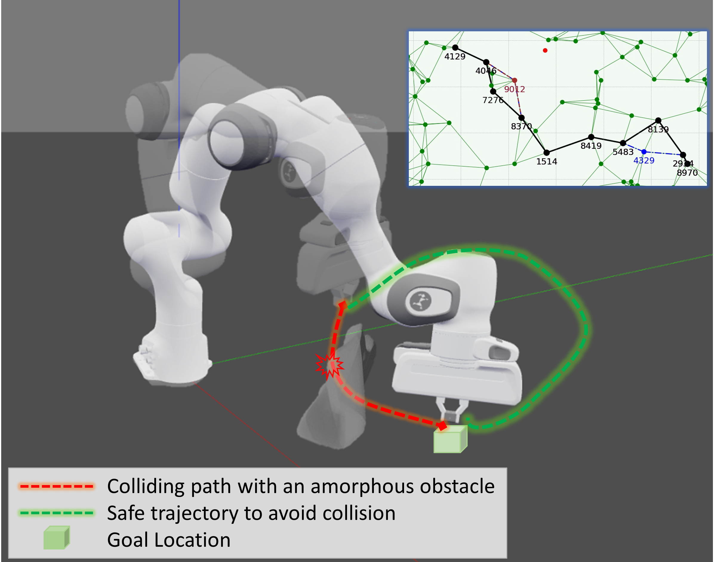
Statement of Contributions: In this paper, we present DAMON, a novel approach to tackle the challenges of robotic arm motion planning. It adopts a topological manifold perspective and adaptive graph traversals to avoid dynamic obstacles, as depicted in Fig.1. Unlike prior works [9, 4, 6, 7] that rely on complex system dynamics modeling or multiple-network sample-based computing on latent space, DAMON employs a unique manifold learning-based framework that adaptively traverses a pre-computed hierarchically-structured graph in a low-dimensional latent space. Our specific contributions are as follows:
(1) DAMON is superior to previous sampling-based methods due to its universal, versatile, and reusable nature. Once learned for a specific robotic manipulator, it can avoid any number of 3D obstacles with arbitrary and unseen trajectories, making it highly applicable in human-robot collaboration applications. Moreover, DAMON can handle any number of dynamic obstacles with arbitrary shapes once the underlying manifold surface is learned. This makes DAMON more adaptable and robust to real-world scenarios where the environment can change unpredictably.
(2) DAMON’s algorithm creates a hierarchically-structured graph for efficient traversal of the latent space. Its ability to encapsulate intricate information about a robotic arm’s interaction with its surroundings in a low-dimensional graph results in faster and more efficient motion planning with lower computational overhead and memory requirements. This scalability and efficiency make it suitable for real-time applications and enable safer human-robot interaction.
(3) DAMON uses Gaussian mixture models for statistical learning, allowing for robust performance evaluation and optimal algorithm parameter selection. Its ability to navigate multiple obstacles while achieving multiple objectives makes it versatile and adaptable. DAMON’s generalizability means that the trained model can be applied to new environments and obstacles without additional training, saving time and computational resources.
(4) DAMON’s effectiveness was demonstrated in both simulated and real-world scenarios, surpassing state-of-the-art methods in terms of efficiency and effectiveness. It was used to avoid dynamic obstacles with arbitrary shapes using a 7-DoF robotic manipulator. The approach learned and replicated complex robot skills, and could handle new obstacles without requiring additional learning efforts.
II Problem Formulation: Motion Planning for Dynamic Obstacle Avoidance
The motion control of a robotic manipulator involves calculating a joint-space trajectory that guides the end-effector to a desired position. The forward kinematic mapping of a -DOF robotic manipulator in an -dimensional task space is a surjective function of the joint-space coordinates, , where and are the task-space and joint-space coordinates, respectively. This nonlinear vector-valued function can be easily formulated using the mechanical design and Denavit-Hartenberg parameters for a given manipulator. However, for most applications, computing the inverse mapping from the task space to the joint space is more important, as it allows us to specify the desired end-effector position. Similarly, we can define an inverse kinematics model as , where is the inverse kinematic mapping.
Our goal is to solve the inverse kinematics equation for the joint-space coordinates that guide the end-effector to a target position. However, solving this equation alone does not guarantee that the calculated trajectory will avoid collisions with obstacles. To address this issue, we formulate the problem of obstacle avoidance as the problem of maximizing the minimum distance between the links of the manipulator and the obstacle.
Let and defines the state space and control input of a robotic manipulator system such that where defines the robot’s state condition at timestep, and carries all information about independent obstacles in the environment. The robotic system evolves through time by following defined discrete-time dynamics of robotic system,
| (1) |
where, defines the functional for discrete-time system evolution. Now, let and defines the free state space and colliding state space of the robot, such that . Now for any initial state and a defined goal state , we aimed at finding a continuous trajectory, , such that the continuous curve between adjacent state space in the planned trajectory remains collision free i.e, . Our algorithm ensured that all trajectory path safely ends at pre-defined goal state .
III Proposed Methodology
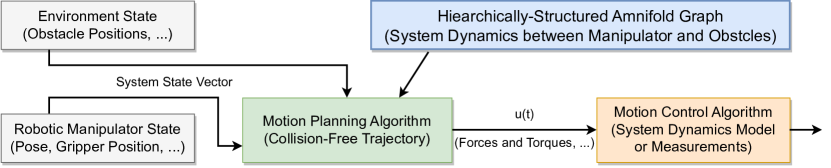
Fig. 2 depicts DAMON, consisting mainly of two algorithm modules: the motion control algorithm (MCA) and the motion planning algorithm (MPA). The MPA module computes an optimized trajectory that satisfies all spatial and temporal requirements, while the MCA generates control signals that regulate the position, velocity, and acceleration of the robotic manipulator’s actuators, allowing the robot manipulator to track the computed trajectory. Although DAMON adopts the conventional PID control for MCA, it focuses on developing an innovative motion planning algorithm that efficiently avoids dynamic obstacles while reaching its objective state. The key idea behind DAMON is to adaptively traverse a hierarchically-structured manifold graph that captures the intricate dynamics of the entire system, including a whole-body robotic arm and a point obstacle located anywhere in the workspace. By doing so, DAMON efficiently avoids dynamic obstacles while achieving its objective state.
DAMON addresses the primary challenge of computational inefficiency and intractability in motion planning for real-world robotic systems. Such systems have complex system dynamics and high-dimensional state-space, making conventional algorithms unsuitable for dynamic environments. Even sampling-based motion planning methods can become inefficient when the state-space evolves randomly after the planner has completed planning. Moreover, sampling-based dynamic replanning algorithms, such as [8, 10], consume a significant amount of runtime to re-sample a new path when dynamic obstacles block the initial path. This inefficiency is further compounded by the fact that the computational load increases as the number of obstacles and dimensions in the workspace grows.
In the following, we provide more information on the three major algorithm modules that constitute DAMON.
Algorithm Module 1: Topological Manifold Learning
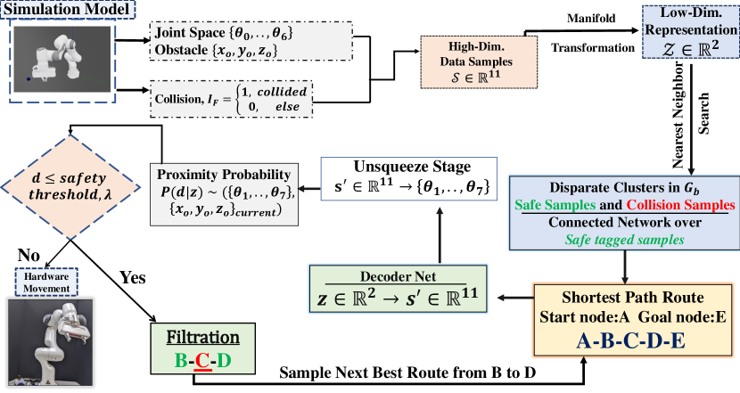
Manifold learning is a mathematical framework used to investigate the geometrical structure of datasets in high-dimensional spaces. In this paper, we consider a high-dimensional space defined by , where determines the full joint-space pose of a robotic arm and defines the location of a point obstacle. is a boolean collision flag. Our key insight of DAMON is that the geometrical structure of this high-dimensional space, combining both the pose of robotic manipulator and the 3D location of obstacle, can encapsulate all the intricate information about how a robotic arm interacts with its surroundings, especially a point obstacle at an arbitrary location, in a low-dimensional latent-space graph. This approach circumvents the need for repeated computation required by obstacle detection and motion replanning. Furthermore, to handle 3D geometrical obstacles, we consider the closest point on the 3D mesh of the object to 3D collision meshes of the robot’s pose as the point obstacle coordinate showed in Figure 7.

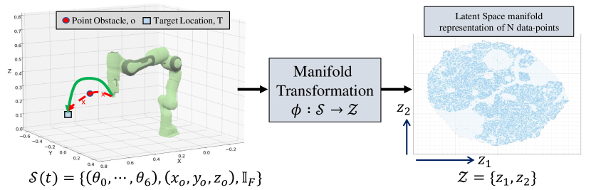
To leverage the embedding power of our learned low-dimensional manifold for robotic motion planning, we need to seamlessly transform between the high-dimensional robotic space, , and the low-dimensional manifold space, . To achieve this, we utilized a variational autoencoder (VAE) [14] for both latent space learning and decoding to the high-dimensional state space. Specifically, as depicted in Fig. 4, our VAE is implemented as a feedforward, non-recurrent neural network that employs an input layer and an output layer connected by multiple hidden layers. The output layer has the same number of nodes (neurons) as the input layer. The purpose of our VAE is to reconstruct its inputs, minimizing the difference between the input and the output, rather than predicting a target value given inputs . This allows us to capture the essential information about the high-dimensional robotic space in a lower-dimensional manifold, enabling us to perform efficient motion planning and obstacle avoidance in real-time. The implementation of VAE in DAMON largely adopted from [10] and is trained through backpropagation of the error. Conceptually, the feature space of our autoencoder is the low-dimension manifold representations produced by manifold learning, therefore having lower dimensionality than the input space , which, in DAMON, is the pose of our 7-DoF robotic manipulator with object position and collision flag. As such, the feature matrix after manifold learning can be regarded as a compressed representation of the input .
Algorithm Module 2: Hierarchical Graph Construction and Graph-Traversal-Based Motion Planning
To achieve robustness and adaptability in motion planning for real-world scenarios where the environment can change unpredictably, DAMON employs two key techniques. Firstly, we learn the latent space manifold representation , where , through a mapping function . Secondly, instead of relying on a sampling-based tree expansion, we construct a fully connected graph , where and is weighted by nearest joint space control inputs for smoother trajectory execution. We utilize for path traversal from any to . Furthermore, the dense connectivity of our graph allows the planner to re-route from any node without significant runtime loss, even if the old path becomes convoluted due to a potential collision with a moving obstacle. These two techniques ensure that DAMON can efficiently handle changing environments while maintaining adaptability and robustness. The latent space manifold representation reduces the dimensionality of the state-space, making it easier to handle and learn. The fully connected graph enables us to utilize the learned representation for efficient path traversal and re-routing, even in dynamic environments with moving obstacles.
Although graph-based robotic motion planning is a well-established technique [15], it is commonly used for mobile robots operating in complex environments[16, 17]. Our DAMON methodology has two distinctions from these graph-based motion planning studies. Firstly, DAMON exploits a two-layered hierarchical graph that encodes the complex system dynamics between a robotic manipulator and its closest obstacle through a topological manifold space. Secondly, DAMON performs adaptive graph traversal for effective motion planning.
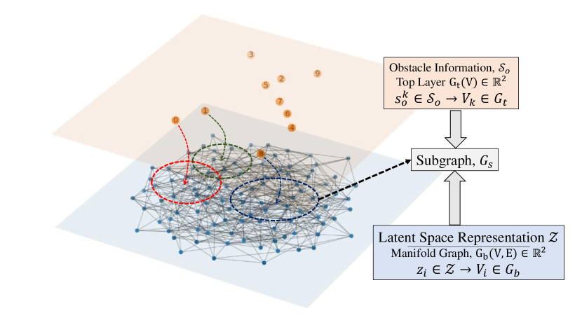
DAMON simplifies its data structure and facilitates graph traversal by leveraging a hierarchically-structured low-dimensional manifold space . In this manifold graph depicted in Figure 6, the bottom layer contains all the manifold points learned from VAE for the stored dataset, with each corresponding to a vertex in the graph layer . The top layer considers the point obstacle information as each node , where is the number of obstacles considered while accumulating the dataset.
To further simplify the structure, the manifold graph is partitioned into multiple subgraphs, each containing all vertices with the same obstacle 3D locations. Conceptually, a hyperedge between the two layers connects the vertices associated with respective . Furthermore, the vertices in each subgraph are labeled as either ”collision” or ”collision-free/safe” samples. During robotic arm motion planning, we use Dijkstra’s algorithm to perform shortest-distance routing, considering only the green vertices (”collision-free/safe”) for safer robot movement.
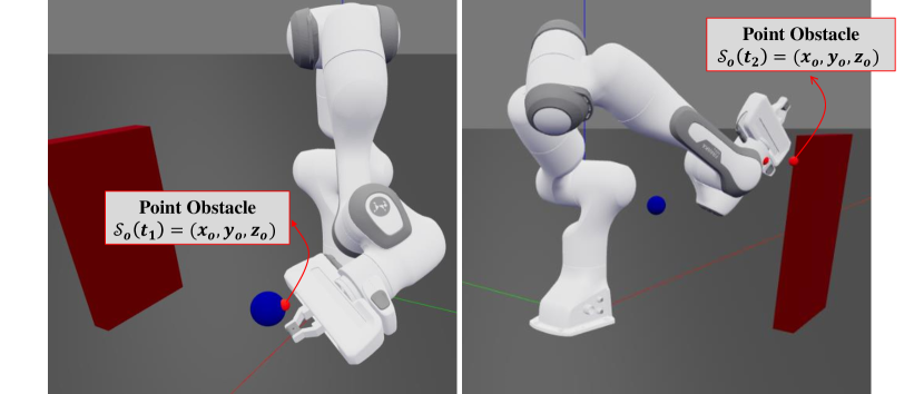
The 2-layer hierarchically-structured manifold graph reduces computational overhead as DAMON only needs to traverse the subgraph in that is closest to the current obstacle point location. We use a KD-Tree to quickly query the node that is closest to the current point obstacle location, as illustrated in Fig. 7. When multiple dynamic obstacles are present, DAMON hops among different subgraphs according to the one closest to the robotic manipulator.
Our implementation manipulates graph-like objects solely via predefined API methods and not by acting directly on the data structure. We utilize the well-known ”dict-of-dicts” structure as the main data structure, which allows fast addition, deletion, and lookup of nodes and neighbors in large graphs. Our software code is based largely on the open-source NetworkX package[18]. We omit the standard implementation details for the sake of brevity.
Algorithm Module 3: Theoretical Framework for Performance Analysis and Algorithm Parameter Optimization
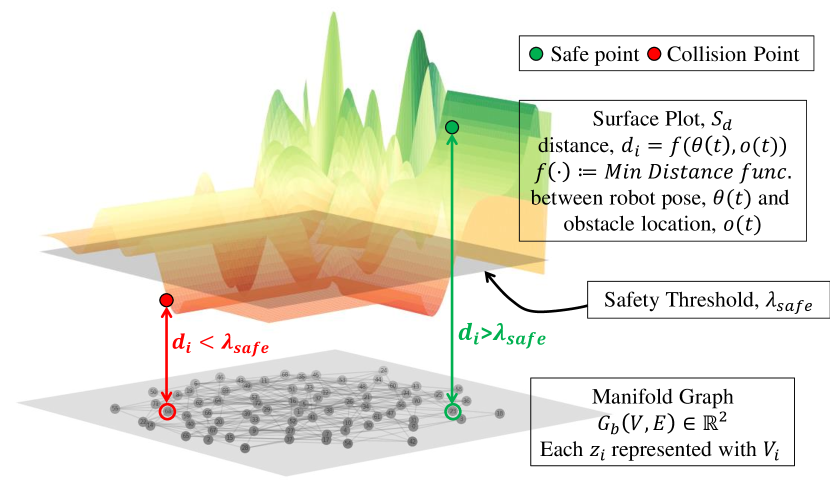
When optimizing the algorithm of DAMON, we need to address two key algorithm questions. Firstly, how to accurately estimate the delay performance of DAMON for a given task and its setting? Secondly, for a given delay performance requirement, what should be the ideal density of our constructed manifold graph? To satisfactorily answer both of these questions, DAMON develops an analytical framework to compute the average rerouting probability and derive the relationship between the total runtime of each robotic experiment and the density of our low-dimensional manifold graph. To this end, DAMON utilizes the Gaussian mixture regression (GMR) [19] to estimate the conditional probability distribution of given a set of input latent space variables, i.e., its manifold coordinates of vertex , as shown in Figure 8.
DAMON assumes that our manifold graph consists of vertices, each of which is denoted by defined by low-dimensional coordinates and augmented with . Abstractly, represents a multivariate functional surface depicted in Fig. 8. With the GMR method, DAMON assumes that the target variable obeys a mixture of Gaussian distributions, where the parameters of each Gaussian component are dependent on the input variables , where . During the training phase, DAMOM learns a -component Gaussian mixture model through Expectation-Maximization (EM) training [19], where are Gaussian distributions with mean and covariance is the number of Gaussians, and are priors that sum up to one. After the Gaussian mixture model is successfully trained, DAMON performs a regression to predict distributions of variables by computing the conditional distribution . The conditional distribution of each individual Gaussian is , where , , , and . DAMON can now compute the conditional distribution of each individual Gaussian and their priors according to to obtain the conditional distribution . Now, given any location on the manifold graph, we can compute its probability of collision as
| (2) | ||||
where is a user-defined parameter that defines the minimum distance required to be collision-free between obstacle and the robotic manipulator.
Let one complete trajectory in DAMON contain vertices , on the manifold surface graph. During each step from , the robotic manipulator will take in total run-time, where and denote the motion planning time for each step and the runtime for the robotic manipulator moving from to , . Note that the multiplying factor of accounts for the rerouting time when traversing causes collision. Therefore, the total runtime for each task trajectory will follow
| (3) |
III-1 Estimating the delay performance of DAMON
DAMON uses the standard EM learning algorithm to extract a Gaussian Mixture Model with statistical accuracy. With in hand, we can easily calculate the probability of collision at any location on the manifold, as indicated by Equation 2. This approach provides an effective means of estimating the total runtime for each trajectory task, as shown in Equation 3. It’s worth noting that we have made two simplifying assumptions. First, we assume that each routing step on the manifold graph is probabilistically independent during each computed trajectory. Second, we assume that the robotic manipulator moves at a constant average rate. These assumptions were made for the sake of brevity in modelling. However, it is possible to achieve more complex modelling to account for variable velocity and acceleration.
III-2 Determining the optimal manifold point density
Intuitively, as the point density of the manifold graph increases, the rerouting probability due to data sparsity error decreases. However, the graph traversing time and the motion planning time in each step are likely to increase because a denser manifold graph requires more computations. Additionally, as the rerouting probability at each manifold vertex decreases, the average number of steps decreases. Hence, there is an intriguing and complicated relationship between the number of manifold points collected and the average runtime for a typical motion trajectory. Our experimental results in Fig. 11 have validated this analytical finding. Equations 2 and 3 together provide an effective way of determining the optimal number of manifold points we need to collect, given a well-defined performance requirement in terms of the total runtime for each task.
IV System Overview
IV-A Experimental Platform and Simulation Setup
In our hardware demonstrations, we utilized a 7-DoF Franka Emika Panda robot arm mounted on a table-top workspace, as depicted in Fig.14. Our adaptive trajectory planning algorithm was implemented in Python and ran on a Lambda QUAD GPU workstation equipped with an Intel Core-i9-9820X processor. To track dynamic obstacles and extract depth information, we used an Intel RealSense Depth Camera D435i. By applying the conventional hand-to-eye calibration mathematical formulation, we transported the information from the camera reference frame to the robot coordinate system. Our algorithm utilized this feedback from depth sensors to avoid obstacles in real-world scenarios by computing the distance between the 3D geometry of the obstacle and the collision meshes of robot links using the Gilbert–Johnson–Keerthi distance (GJK)[13] algorithm to safely route to the target location. To validate our approach, we replicated the exact model of the Franka Emika Panda Arm in Robotics Toolbox (RTB) for Python. We encapsulated the entire framework inside the Robot Operating System (ROS) ecosystem, utilizing libfranka and Franka ROS, to establish low-latency and low-noise communication protocols for data processing and parallel execution among simulation environments and real hardware.
IV-B Experimental Procedures and Learning Variables
We collected high-dimensional data samples from the robot’s workspace and transformed them into a latent space representation for creating the topological manifold. Each data sample contained 11 numerical variables, including 7 joint angles, the position of a point obstacle in 3D space, and a binary collision flag. We accumulated a dataset of 1MM samples by randomly manipulating the arm in the simulated environment for a large number of epochs. Our VAE architecture, implemented on PyTorch [20], had a decoder and encoder network with three layers containing (300, 200, 75) neurons and an encoded latent space representation in . We focused on collecting adequate collision samples to ensure a safer elementary trajectory. When the algorithm and manifold learning converged, we conducted real-time and scalable test experiments against varying occlusions created by geometrically different 3D objects in the real hardware setup.
V Results Analysis
Our experiments seek to investigate the following:
-
1.
Can DAMON learn manifold representation space differentiating the non-colliding and colliding samples with hierarchical structure for faster routing?
-
2.
Can we preserve the best performance model with optimal and computationally efficient sample density for efficient graph routing while reducing the rerouting probability?
-
3.
Can DAMON concurrently track the unseen perturbations created by geometrically varying obstacles and dynamically adjust the trajectory to reach the goal location through graph routing?
V-A Latent-Space Manifold Graph and Optimum Routing
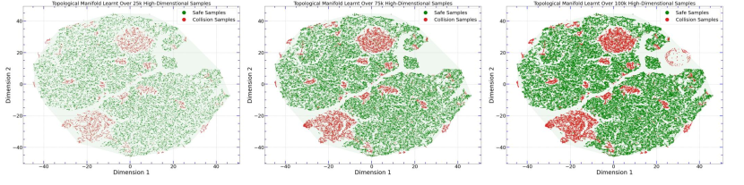
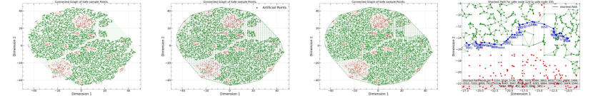
Each input sample in DAMON’s high-dimensional space comprises the joint angle vector for the robotic manipulator in operation, the 3D coordinate location of the closest point on the obstacle mesh, and a collision flag . Our Variational Autoencoder (VAE) learns a topological manifold representation from this high-dimensional space. As illustrated in Fig. 9, the latent space manifold representation exhibits visually contrasting clusters based on the binary level of the collision flag. Next, we construct a connected graph, , over the space that contains only the collision-free samples. By applying the unsupervised -Nearest Neighbor algorithm [21] to locate the nearest family of vertices in the collision-free manifold space, we create a connected graph that accelerates any shortest path routing algorithm to traverse on a transformed low-dimensional manifold graph. We further divide the large graph, , into several subgraphs, , where each is associated with its own obstacle information embedded in the top layer of the hierarchical graph structure. As depicted in Fig.10(a), disconnected sub-networks are automatically generated inside the safe manifold while creating connected graphs, as the nearest neighboring algorithm only helps to create a connected network at the closest distance. This sub-network generation violates the notion of a complete path routing from any random node to another random node on the fully connected network. To ensure dense connectivity, we artificially sample points in the same space as a grid mesh over the learned space. By adjusting the level of sparsity in creating the grid of artificial points, we can easily sample denser artificial points to create a densely connected network. With the decoder part of our trained VAE, we can label these artificial points as safe/colliding sample points, as shown in Fig.10(c). Furthermore, with decoded high-dimensional points, we can label these artificial points to their nearest obstacle node of and include them in the associated subgraph networks.
| Methods | Environment Settings | Environment Settings | Obstacle Condition | ||||||||||||||
| Total Runtime, T (s) | Smoothness Comparison | Success Ratio (%SR) | |||||||||||||||
| A | B | C | D | E | A | B | C | D | E | Static | Dynamic | ||||||
| DAMON | 3.2 | 4.7 | 5.1 | 6.5 | 7.3 | 0.31 | 0.35 | 0.41 | 0.57 | 0.51 | 98.6 | 97.8 | |||||
| RRT | 42.5 | 39.2 | 46.3 | - | - | 0.25 | 0.25 | 0.25 | - | - | 78.4 | - | |||||
| RRT* | 22.6 | 20.4 | 29.6 | - | - | 0.61 | 0.81 | 0.55 | - | - | 83.2 | - | |||||
| Dynamic-RRT* | 15.1 | 13.4 | 15.9 | 37.2 | 45.2 | 0.55 | 0.67 | 0.41 | 0.91 | 0.84 | 86.2 | 76.3 | |||||
| L2RRT | 7.9 | 6.2 | 8.3 | - | - | 0.35 | 0.38 | 0.39 | - | - | 90.2 | - | |||||
| MpNet | 5.6 | 6.1 | 7.2 | 10.3 | 12.85 | 0.42 | 0.53 | 0.64 | 0.88 | 0.95 | 91.3 | 82.3 | |||||
| Environment Settings Details: | |||||||||||||||||
|
|
||||||||||||||||
V-B Performance Analysis and Comparison to Baselines
We evaluate the performance of DAMON against classical navigation approaches and state-of-the-art latent-space sampling-based algorithms with the following metrics:
-
•
Total Runtime, : Total Runtime is determined by calculating total time to compute the initial path, ; time to maneuver by the physical robot joints, ; time to perform replanning if the initial path gets occluded with dynamic obstacle, ;
-
•
Success Ratio, : A planned trajectory is successful if the robotic arm reaches the target location without colliding with any moving obstacles.
-
•
Trajectory Smoothness: Smoothness will be measured by summing up the joint space configuration change in consecutive via-point pair along the planned path, i.e , where N is the total number of movement stages.
Table II showcases the performance of DAMON in comparison to other main methods. To ensure thoroughness, we have tested DAMON in 5 different settings that involve both static and dynamic obstacles to verify its generalization capability. It is worth noting that RRT, RRT*, and L2RRT do not explicitly support dynamic obstacle replanning; hence, their results against dynamic environments are unavailable. Regarding total runtime, DAMON outperforms other approaches by 2-3 times on average across all cases. However, when it comes to trajectory and movement smoothness, the comparison results are mixed. In general, DAMON is smoother than RRT* Dynamic RRT*, and MpNet, but less smooth than RRT, and about the same as L2RRT. We believe that this discrepancy is primarily due to the sampling-intensive nature of computing versus relatively more efficient graph traversal. Finally, in terms of navigation success rate, DAMON clearly demonstrates its edge over all other methods. We attribute this mostly to the synergistic interplay between topological manifold learning and adaptive graph traversal.

Furthermore, Fig. 11 plots how the number of samples affects the total runtime and the aggregated rerouting probabily in DAMON across 12 different obstacle scenarios. When tested against with the analytic performance framework in Section III, our experimental results have shown a close match. For both cases, larger number of sampling points to form our manifold graph will in general make the graph traversal more successful and rerouting less needed. However, denser manifold graph also requires more computation, thus long per-stage motion planning time. As such, there is an intriguing and complicated interplay between the density of manifold graph and performance metrics. To balance this trade-off between readily available safe path for rerouting and initial trajectory over optimal number of nodes , we found the optimal number of nodes which produced the lowest average over set of different test-cases. Lastly, Figure 11 showed how the rerouting probability plateaued to a fixed range as we consistently increased the number of samples while computing rerouting probability. This convergence of rerouting probability pointed out that we located which allowed required amount of rerouting capability without increasing additional computational overhead for our graph-centric navigation planning.
V-C Adaptive Navigation with Dynamic Obstacle Avoidance
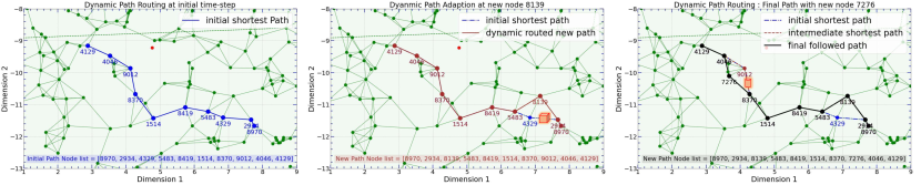
DAMON achieves dynamic obstacle avoidance on a 2-D manifold graph, by adapting the trajectory in real-time to reach the goal position as quickly as possible while avoiding moving obstructions. The system achieves this by receiving feedback based on distance measurements and adapting its path using a nearest neighbor network. It is worth noting that each manifold vertex in DAMON contains not only the pose state of the robotic arm and a specific point obstacle, but also the precomputed distance between the obstacle and the robotic manipulator. This precomputed information and the topology of manifold graph is crucial because it embeds the intricate dynamics between the robotic arm and the obstacle, effectively minimizing the computing effort required for on-the-fly motion planning.
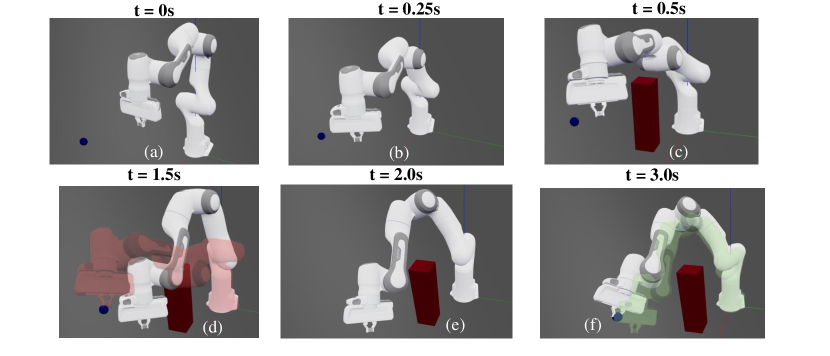
We demonstrate the effectiveness of our proposed method in achieving dynamic obstacle avoidance with Fig. 12. Initially, the robotic arm attempted to reach the goal position by following its initial computed trajectory. However, at a later time step, as shown in Fig. 12(c), a dynamically placed obstacle blocked the robot’s motion. DAMON effectively guided the robotic arm to re-route through a new trajectory, which successfully dodges the obstacle and move around the red block, thus avoiding a possible collision and successfully reaching the target position. With extensive experimentations, as listed in Table II, DAMON has shown to be capable of efficiently adapting the robot manipulator’s trajectory in real-time, enabling it to avoid moving obstructions and reach its destination safely.
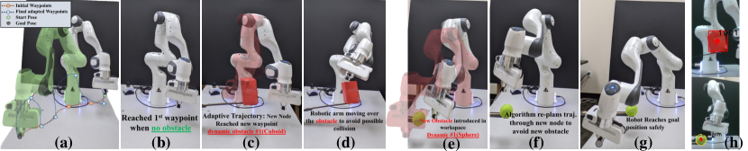
Since DAMON leverages only point obstacle information for replanning, our proposed approach can be easily extended for avoiding probable collision with any shaped obstacles. In Fig. 13, we attempted to graphically convey an idea on how DAMON successfully performed replanning when the robot’s initial motion was convoluted with presence of different shaped obstacles. For instance, the routing performed successfully even when the 3D shape of obstacles varied between a cuboid mesh and cylindrical mesh. Inside the RTB simulated environment, integrated high functionality API can be effortlessly used to track the proximal distance among 3D meshes. This API has been modified with the GJK algorithm [13] for calculating the proximity among 3D meshes in real-world scenarios. This distance metric produced a feedback to the controller when the robot’s mechanical structure reaches very close to an obstacle. When there is chance of probable collision i.e , the robot controller is triggered to halt its current trajectory motion and revise its intermediate node connectivity to reach the preset goal position. On hardware setup, we localized obstacles in consecutive frames by applying color filtering through HSV color model and tracked the spatial positions of random obstacles through depth information extracted from Realsense depth camera. After successful extraction of depth values, we transported the 3D coordinate value of closest point on the object mesh to the learning controller and the controller evaluated the probability of collision based on our GMM model. If the condition is suddenly violated, the algorithm replans for a new shortest and safest path to reach the goal position. In Fig. 14, we have added snapshots from real hardware operation. In red shaded figure, we also depicted the probable collision would occur without the presence of dynamic adaption on real time. Here, we validated our experiments with varying size and different geometric objects. For both obstacles, our adaptive motion planning approach successfully avoided the dynamic obstacles which appear at different time-step of robot operation.
VI Conclusion
Dynamically avoiding 3D obstacles with unpredictable trajectories for a given robotic manipulator can be effectively addressed by combining three theoretical algorithm modules - topological manifold learning, variational autoencoding, and adaptive graph traversing. By reducing dynamic obstacle avoidance to a basic point obstacle avoidance problem supported by a strong theoretical foundation, DAMON demonstrates versatility and generalizability in tackling arbitrary numbers of obstacles.
References
- [1] M. A. Goodrich and A. C. Schultz, “Human-robot interaction: A survey,” Foundations and Trends in Human-Computer Interaction, vol. 1, no. 3, pp. 203–275, 2007.
- [2] P. S. Schmitt, F. Witnshofer, K. M. Wurm, G. V. Wichert, and W. Burgard, “Modeling and planning manipulation in dynamic environments,” Proceedings - IEEE International Conference on Robotics and Automation, vol. 2019-May, pp. 176–182, 2019.
- [3] D. Falanga, K. Kleber, and D. Scaramuzza, “Dynamic obstacle avoidance for quadrotors with event cameras,” Science Robotics, 2020.
- [4] S. Sundar and Z. Shiller, “Optimal obstacle avoidance based on the hamilton-jacobi-bellman equation,” IEEE Transactions on Robotics and Automation, vol. 13, no. 2, pp. 305–310, 1997.
- [5] S. M. Khansari-Zadeh and A. Billard, “A dynamical system approach to realtime obstacle avoidance,” Autonomous Robots, vol. 32, no. 4, pp. 433–454, 2012.
- [6] L. Blackmore, M. Ono, and B. C. Williams, “Chance-constrained optimal path planning with obstacles,” IEEE Transactions on Robotics, vol. 27, no. 6, pp. 1080–1094, 2011.
- [7] A. Garg, H.-T. L. Chiang, S. Sugaya, A. Faust, and L. Tapia, “Comparison of deep reinforcement learning policies to formal methods for moving obstacle avoidance,” IEEE/RSJ International Conference on Intelligent Robots and Systems (IROS), pp. 3534–3541, 2019.
- [8] O. Adiyatov and H. A. Varol, “A novel rrt*-based algorithm for motion planning in dynamic environments,” in 2017 IEEE International Conference on Mechatronics and Automation, 2017, pp. 1416–1421.
- [9] B. Ichter and M. Pavone, “Robot motion planning in learned latent spaces,” IEEE Robotics and Automation Letters, vol. 4, no. 3, pp. 2407–2414, 2019.
- [10] A. H. Qureshi, Y. Miao, A. Simeonov, and M. C. Yip, “Motion planning networks: Bridging the gap between learning-based and classical motion planners,” IEEE Transactions on Robotics, vol. 37, no. 1, pp. 48–66, 2021.
- [11] H. B. Mohammadi, S. Hauberg, G. Arvanitidis, G. Neumann, and L. D. Rozo, “Learning riemannian manifolds for geodesic motion skills.”
- [12] A. V. Bernstein, “Manifold learning in machine vision and robotics,” in International Conference on Machine Vision, 2017.
- [13] A. H. Khan, S. Li, and X. Luo, “Obstacle Avoidance and Tracking Control of Redundant Robotic Manipulator: An RNN-Based Metaheuristic Approach,” IEEE Transactions on Industrial Informatics, vol. 16, no. 7, pp. 4670–4680, 2020.
- [14] M. W. Diederik P Kingma, “Auto-encoding variational bayes,” 2014.
- [15] T. Dang, F. Mascarich, S. Khattak, C. Papachristos, and K. Alexis, “Graph-based path planning for autonomous robotic exploration in subterranean environments,” in 2019 IEEE/RSJ International Conference on Intelligent Robots and Systems (IROS), 2019, pp. 3105–3112.
- [16] O. Kupervasser, H. Kutomanov, M. Mushaelov, and R. Yavich, “Using diffusion map for visual navigation of a ground robot,” Mathematics, vol. 8, no. 12, 2020.
- [17] Y. F. Chen, S.-Y. Liu, M. Liu, J. Miller, and J. How, “Motion planning with diffusion maps,” 10 2016.
- [18] A. A. Hagberg, D. A. Schult, and P. J. Swart, “Exploring network structure, dynamics, and function using networkx,” in Proceedings of the 7th Python in Science Conference, G. Varoquaux, T. Vaught, and J. Millman, Eds., Pasadena, CA USA, 2008, pp. 11 – 15.
- [19] Z. Ghahramani and M. Jordan, “Supervised learning from incomplete data via an em approach,” in Advances in Neural Information Processing Systems, J. Cowan, G. Tesauro, and J. Alspector, Eds., vol. 6. Morgan-Kaufmann, 1993.
- [20] A. Paszke, S. Gross, F. Massa, A. Lerer, J. Bradbury, G. Chanan, T. Killeen, Z. Lin, N. Gimelshein, L. Antiga, A. Desmaison, A. Kopf, E. Yang, Z. DeVito, M. Raison, A. Tejani, S. Chilamkurthy, B. Steiner, L. Fang, J. Bai, and S. Chintala, “Pytorch: An imperative style, high-performance deep learning library,” in Advances in Neural Information Processing Systems 32, H. Wallach, H. Larochelle, A. Beygelzimer, F. d'Alché-Buc, E. Fox, and R. Garnett, Eds. Curran Associates, Inc., 2019, pp. 8024–8035.
- [21] P. Cunningham and S. J. Delany, “k-Nearest Neighbour Classifiers: 2nd Edition (with Python examples),” arXiv e-prints, p. arXiv:2004.04523, Apr. 2020.