NORDITA-2022-018 UPPSALA-19/22

Radiation reaction for spinning black-hole scattering
Francesco Alessio^a,b and Paolo Di Vecchia^a,c

^a NORDITA, KTH Royal Institute of Technology and Stockholm University,
Hannes Alfvéns väg 12, SE-11419 Stockholm, Sweden
^b Department of Physics and Astronomy, Uppsala University,
Box 516, SE-75120 Uppsala, Sweden

^c The Niels Bohr Institute, Blegdamsvej 17, DK-2100 Copenhagen, Denmark

Starting from the leading soft term of the $5$-point amplitude, involving a graviton and two Kerr black holes, that factorises into the product of the elastic amplitude without the graviton and the leading soft factor, we compute the infrared divergent contribution to the imaginary part of the two-loop eikonal. Then, using analyticity and crossing symmetry, we determine the radiative contribution to the real part of the two-loop eikonal and from it the radiative part of the deflection angle for spins aligned to the orbital angular momentum, the loss of angular momentum and the zero frequency limit of the energy spectrum for any spin and for any spin orientation. For spin one we find perfect agreement with recent results obtained with the supersymmetric worldline formalism.

1 Introduction

The recent detection of gravitational waves (GW) by the LIGO and Virgo collaborations [1, 2, 3, 4, 5, 6, 7] emitted by binary black holes or neutron stars mergers is shedding new light on the nature of strongly gravitating systems existing in the universe. The increasing sensitivity of the detectors demands for an effort to develop new theoretical tools capable of high-precision predictions of GW waveform templates. For these reasons, recently there has been considerable interest in the use of amplitude-based techniques for studying the inspiral phase of binary non-spinning massive objects coalescence, extracting the conservative part of the Effective-One-Body (EOB) potential [8, 9, 10, 11, 12, 13, 14, 15, 16, 17, 18, 19, 20, 21], classical observables [13, 22, 23, 24, 25], waveforms and radiation [26, 21, 27, 28, 20, 29, 30]. Astrophysical objects are also characterized by their spin. Therefore, the post-Minkowskian (PM) expansion in the Newton’s constant $G$ for studying the scattering of spinning objects has also received attention, using amplitudes methods and classical General Relativity (GR) analytical techniques [31, 32, 33, 34, 35, 36, 37, 38, 39, 40, 41, 42, 43, 44, 45, 46, 47, 48, 49, 50, 51, 52, 53, 54, 55, 56, 57, 58, 59, 60, 61, 62, 63, 64, 65]. Furthermore, observables computed for scattering events in the PM expansion can be compared with those computed in the more traditional post-Newtonian (PN) [66] perturbation theory (for spin effects in the PN scheme see e.g. [67, 68, 69, 70, 71, 72, 73, 74, 75, 76]), which is more suitable for describing bound orbits, using the so-called Bound-to-Boundary (B2B) [16, 17, 18] correspondence.

The contribution of the radiation reaction in the scattering of two spinless black holes at 3PM has been crucial [77] to get rid of the divergence at high energy that appears in the conservative part of the deflection angle [78, 79, 80]. This has been first shown in massive ${\cal{N}}=8$ supergravity by performing the explicit calculation in the soft region [77] instead of just the conservative region [81]. Immediately after the radiation reaction was also computed in GR with two different methods. The first, discussed in Ref. [82], is based on the computation of the loss of angular momentum that is then inserted in a formula derived in Ref. [83] that gives the radiative part of the deflection angle. The second one [84] uses instead the leading soft part of the $5$-point amplitude for the emission of a graviton that allows to compute the infrared divergent contribution to the imaginary part of the eikonal at 3PM order. Then, using considerations based on analyticity and crossing symmetry, the real part of the radiative eikonal at 3PM is also extracted and from it the radiation reaction part of the deflection angle at 3PM has been obtained. The two approaches give the same result that, at high energy, is also in agreement with the old result of Ref. [85]. This result is also confirmed [86, 87, 88] by extracting from the explicit two-loop calculations the radial action and from it the deflection angle.

In this paper we generalise the approach of Ref. [84] to the case of Kerr black holes obtaining a closed expression for the radiation reaction part of the deflection angle in the aligned-spin case and to all order in spin. Assuming that the logarithmic divergence appearing in the radiation reaction contribution to the scattering angle in the ultra-relativistic limit cancels with that appearing in its conservative part, we conjecture a formula describing the high-energy limit of the latter. Furthermore, using the Bini-Damour linear response equation [83, 82, 89], we find the angular momentum loss for any spin configuration and to all orders in spin. Our formula, for spin one, agrees with the one computed in Ref. [55, 62].Furthermore, it is also consistent with the general result for the angular momentum loss obtained in Ref. [90].

The paper is organized as follows. We start in section 2 by introducing the kinematical setup describing the elastic $(2\rightarrow 2)$ and inelastic $(2\rightarrow 3)$ scattering processes under considerations and by showing the corresponding tree-level four-point and five-point amplitudes. We approximate the latter by using Weinberg’s soft graviton theorem, that allows to factorize it in terms of the four-point amplitude and the leading soft factor. In section 3 we introduce the main ideas of our computation and then we proceed to explicitly calculate the infrared divergent contribution to the imaginary part of two-loop eikonal $\delta_{2}$ using the three-particle unitarity cut. Then from it, using analyticity and crossing symmetry, we derive the radiation reaction piece of the real part of $\delta_{2}$. Our result shows that all the spin dependence is encoded in a single vector field, denoted by $\mathbf{f}$ in (3.14). We discuss how this feature can be understood in terms of a Newman-Janis shift [91], which relates the Kerr to the Schwarzschild solution. We end section 3 by displaying the zero-frequency limit of the emitted energy spectrum. In section 4 we determine the radiative contribution to the 3PM deflection angle for an aligned-spin configuration and the 2PM angular momentum loss in any spin configuration. Our final equations (4.6), (4.8) and (4.9) hold to all orders in spin. We close in section 5 with a short summary and an outlook. In this paper we use the mostly plus signature $\eta_{\mu\nu}=\mathrm{diag}(-1,1,1,1)$ and we mainly follow the conventions used in [84].

2 Tree-level four-point and soft five-point amplitudes

We start by considering the tree-level $4$-point amplitude for elastic scattering of two Kerr black holes with masses $m_{1}$ and $m_{2}$ anxd rescaled spin vectors $a_{1}^{\mu}=S_{1}^{\mu}/m_{1}$ and $a_{2}^{\mu}=S_{2}^{\mu}/m_{2}$, that can be written in an exponentiated form as [37, 39, 41]

$$\mathcal{A}^{\mathrm{tree}}_{4}(q)=-\frac{\kappa^{2}m^{2}_{1}m^{2}_{2}}{t}\sigma^{2}\sum_{\pm}(1\pm v)^{2}\mathrm{exp}\bigg{(}\pm i\frac{\epsilon_{\mu\nu\alpha\beta}q^{\mu}a^{\nu}p_{1}^{\alpha}p_{2}^{\beta}}{m_{1}m_{2}\sigma v}\bigg{)}+\mathcal{O}(t^{0}),$$ (2.1)

where in the amplitude with one-graviton exchange we keep only terms non-analytic for $t=-q^{2}\sim 0$ that are relevant for long-range effects. Here $\kappa=\sqrt{8\pi G}$ where $G$ is the Newton constant, $a=a_{1}+a_{2}$, $p_{1}$ and $p_{2}$ are the incoming momenta, $q=-p_{1}-p_{4}=p_{2}+p_{3}$ is the transferred momentum and $\sigma=\frac{1}{\sqrt{1-v^{2}}}=-\frac{p_{1}\cdot p_{2}}{m_{1}m_{2}}$. The amplitude in (2.1), which is the main building block of our analysis, can be obtained by gluing two massive spinning three-point amplitudes at minimal coupling [31, 34, 39], as shown in Fig.1.

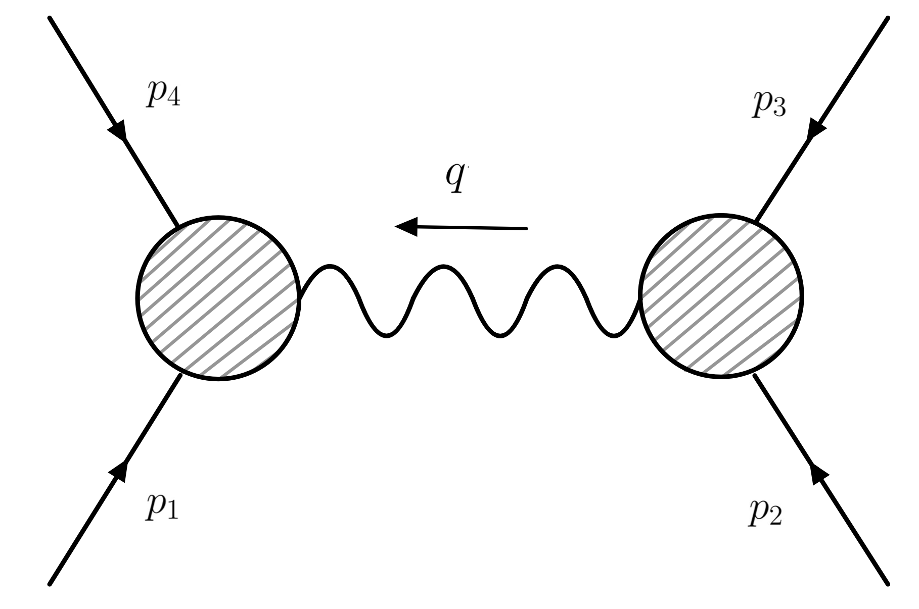
Figure 1: t-channel for the one-graviton exchange.

Note that we treat all vectors as formally ingoing. We work in the center-of-mass frame, defined by

$$p_{1}=(E_{1},\mathbf{p}),\qquad p_{2}=(E_{2},-\mathbf{p}),\qquad\left|\mathbf{p}\right|=p,$$ (2.2)

where $E_{i}=\sqrt{m^{2}_{i}+p^{2}}$ and the total energy, $E=E_{1}+E_{2}=\sqrt{s}$ ($s$ being the Mandelstam variable $s=-(p_{1}+p_{2})^{2}$), satisfies $Ep=m_{1}m_{2}\sqrt{\sigma^{2}-1}$. The spin vectors are given by

$$a_{1}=\bigg{(}\frac{\mathbf{p}\cdot\mathbf{a}_{1}}{m_{1}},\mathbf{a}_{1}+\frac{\mathbf{p}\cdot\mathbf{a}_{1}}{m_{1}(m_{1}+E_{1})}\mathbf{p}\bigg{)},\quad a_{2}=\bigg{(}-\frac{\mathbf{p}\cdot\mathbf{a}_{2}}{m_{2}},\mathbf{a}_{2}+\frac{\mathbf{p}\cdot\mathbf{a}_{2}}{m_{2}(m_{2}+E_{2})}\mathbf{p}\bigg{)},$$ (2.3)

so that $a_{i}^{2}=\mathbf{a}_{i}^{2}$. We choose the spatial component of the momenta and of the impact parameter to be along the $x^{3}$ and $x^{1}$ directions, respectively, i.e. $\mathbf{p}=p\,\mathbf{e}_{3}$ and $\mathbf{b}=b\,\mathbf{e}_{1}$, so that the asymptotic scattering plane is the $x^{1}x^{3}$ plane. Here $\mathbf{e}_{i}$ are the Cartesian spatial unit vectors. So far we have not specified the directions of the spatial spin vectors $\mathbf{a}_{i}$. If we choose them to be perpendicular to the $x^{1}x^{3}$ plane we are considering an aligned-spin configuration. However we will leave these directions arbitrary in the following, unless otherwise specified.

The exponential factor appearing in the amplitude (2.1) in the center-of-mass frame can be expressed in terms of spatial vectors only as

$$\pm i\frac{\epsilon_{\mu\nu\alpha\beta}q^{\mu}a^{\nu}p_{1}^{\alpha}p_{2}^{\beta}}{m_{1}m_{2}\sigma v}=\pm i\mathbf{q}\cdot(\hat{\mathbf{p}}\times\mathbf{a}),\qquad\hat{\mathbf{p}}=\frac{\mathbf{p}}{p},$$ (2.4)

where $\mathbf{q}$ is the $2$-dimensional spatial transferred momentum satisfying $\mathbf{q}\cdot\mathbf{p}=0$ ($\epsilon_{0123}=1$). We now consider the inelastic $(2\rightarrow 3)$ process with the emission of an additional graviton of momentum $k$ and we denote the corresponding $5$-point amplitude by $\mathcal{A}_{5}^{\mu\nu}(q,k)$. We use the following parametrisation for the momenta

$$p_{1}\simeq\bar{p}_{1}-\frac{1}{2}q,\quad p_{2}\simeq\bar{p}_{2}+\frac{1}{2}q,\quad p_{3}\simeq-\bar{p}_{2}+\frac{1}{2}q,\quad p_{4}\simeq-\bar{p}_{1}-\frac{1}{2}q,$$ (2.5)

where $p_{1}^{2}=m^{2}_{1}\simeq\bar{p}^{2}_{1}$, $p_{2}^{2}=m_{2}^{2}\simeq\bar{p}^{2}_{2}$ and $\bar{p}_{1}\cdot q\simeq 0$, $\bar{p}_{2}\cdot q\simeq 0$ hold up to terms proportional to $k$, which are negligible in the soft $k\rightarrow 0$ limit. In this regime, the five point amplitude for such process factorizes according to Weinberg soft graviton theorem [92] as

$$\mathcal{A}_{5}^{\mu\nu}(q,k)=\kappa\sum_{i=1}^{4}\frac{p_{i}^{\mu}p_{i}^{\nu}}{k\cdot p_{i}}\mathcal{A}^{\mathrm{tree}}_{4}(q)+\mathcal{O}(k^{0}).$$ (2.6)

The multiplicative factor is the so-called Weinberg pole, that diverges as $k^{-1}$ for small $k$. In general, one could go further in the soft expansion and consider subleading soft terms with higher powers of $k$ [93, 94]. However, since we shall only be concerned in the infrared divergent part of the imaginary part of the two-loop eikonal $\delta_{2}$, which is responsible for radiation reaction effects [84, 30], we can neglect all such terms and consider contributions that come only from those diagrams where the graviton line is attached to an external leg.

By taking the classical limit, corresponding to $q\rightarrow 0$, and therefore expanding the soft factor in powers of $q$ and keeping only the terms linear in $q$, equation (2.6) becomes

$$\mathcal{A}_{5}^{\mu\nu}(q,k)=\kappa\bigg{(}\frac{\bar{p}_{1}^{\mu}\bar{p}_{1}^{\nu}}{(\bar{p}_{1}\cdot k)^{2}}(q\cdot k)-\frac{(\bar{p}_{1}^{\mu}q^{\nu}+\bar{p}_{1}^{\nu}q^{\mu})}{\bar{p}_{1}\cdot k}-1\leftrightarrow 2\bigg{)}\mathcal{A}_{4}^{\mathrm{tree}}(q)+\mathcal{O}(q^{2},k^{0}).$$ (2.7)

where we have dropped higher powers of $q$ that are negligible in the classical limit.

3 Infrared divergence of the two-loop eikonal

In this section we first go to impact parameter space and then we compute the infrared divergent contribution to the unitarity relation given by the three-particle cut that provides the imaginary part of the two-loop eikonal. Then following the analysis based on crossing symmetry and analyticity discussed in Refs. [77, 84, 30] we can extract the radiation reaction contribution to the real part of the eikonal by means of the relation

$$\mathrm{Re}\,2\delta_{2}^{\mathrm{rr}}=-\lim_{\epsilon\to 0}[\pi\epsilon(\mathrm{Im}\,2\delta_{2})],$$ (3.1)

where $\epsilon=\frac{4-D}{2}$. Equation (3.1) has been confirmed by explicit two-loop calculations in massive ${\cal{N}}=8$ supergravity and in GR [30] and is believed to hold at all energies and for all gravitational theories involving two derivatives. As a consequence of (3.1), the infrared divergent part of the tree-level, on-shell, inelastic amplitude for the $(2\rightarrow 3)$ process under consideration, which is simply fixed in (2.7) by the leading Weinberg soft graviton theorem, is the only necessary ingredient to study radiation reactions effects [84, 95]. This method provides a powerful shortcut to get information about $\mathcal{O}(G^{3})$ classical observables, which are usually obtained by a more involved two-loop computation. In particular, the two observables that one can extract from Eq. (3.1) are the zero-frequency limit of the emitted energy spectrum [96] and the radiative contribution to the 3PM scattering angle given by

$$\left.\frac{dE^{\mathrm{rad}}}{d\omega}\right|_{\omega\to 0}=\lim_{\epsilon\to 0}[-4\hbar\epsilon(\mathrm{Im}\,2\delta_{2})],\qquad\theta^{\mathrm{rr}}_{3}=-\frac{\hbar}{p}\frac{\partial\mathrm{Re}\,2\delta_{2}^{\mathrm{rr}}}{\partial b}.$$ (3.2)

Furthermore, having determined $\theta_{3}^{\mathrm{rr}}$ from Eq. (3.2) and assuming the Bini-Damour linear response equation [83, 82, 89, 97, 98] that gives it in terms of the angular momentum $J^{\mathrm{loss}}$ and the conservative deflection angle $\theta^{\mathrm{cons}}$,

$$\theta^{\mathrm{rr}}=-\frac{1}{2}\frac{\partial\theta^{\mathrm{cons}}}{\partial E}E^{\mathrm{loss}}-\frac{1}{2}\frac{\partial\theta^{\mathrm{cons}}}{\partial J}J^{\mathrm{loss}},$$ (3.3)

where $J=bp$ is the initial angular momentum in the center-of-mass frame, one can extract, inverting (3.3) and discarding the contribution of the energy loss that starts at $\mathcal{O}(G^{3})$, the contribution to the angular momentum loss at $\mathcal{O}(G^{2})$, denoted here by $J^{\mathrm{loss}}_{2}$, which is entirely given by zero-frequency gravitons [90].

Note that the scattering angle can be only defined in the aligned-spin configuration. Indeed, when the two spin vectors are not aligned, the scattering dynamics is not planar and the asymptotic scattering planes at $t=-\infty$ and $t=\infty$ will not coincide and there are rather two scattering angles [49]. In this case, the angular momentum in the center-of-mass frame is radiated in both directions orthogonal to $\mathbf{p}$ [59]. In our kinematics setup described after equations (2.3), it means that the radiated angular momentum has non-vanishing components along $x^{1}$ and $x^{2}$. In the rest of this section we compute the infrared divergent part of $\mathrm{Im}\,2\delta_{2}$.

We first take the leading soft $5$-point amplitude in Eq. (2.7) and we go to impact parameter space by the following formula:

$$\tilde{\mathcal{A}}_{5}^{\mu\nu}(b,k)=\int\frac{d^{4-2\epsilon}q}{(2\pi)^{4-2\epsilon}}e^{iq\cdot b}\hat{\delta}(2q\cdot\bar{p}_{1})\hat{\delta}(2q\cdot\bar{p}_{2})\mathcal{A}^{\mu\nu}_{5}(q,k),$$ (3.4)

where $\hat{\delta}(2q\cdot\bar{p}_{i})\equiv 2\pi\delta(2q\cdot\bar{p}_{i})$ enforces the orthogonality conditions $q\cdot\bar{p}_{i}=0$. Because of the two $\delta$-functions the integral over the two longitudinal components spanned by $\bar{p}_{i}$ can be easily performed and one arrives at

$$\tilde{\mathcal{A}}^{\mu\nu}_{5}(b,k)=\frac{1}{4m_{1}m_{2}\sqrt{\sigma^{2}-1}}\int\frac{d^{2-2\epsilon}\mathbf{q}}{(2\pi)^{2-2\epsilon}}e^{i\mathbf{q}\cdot\mathbf{b}}\mathcal{A}^{\mu\nu}_{5}(\mathbf{q},k).$$ (3.5)

Inserting the amplitude (2.7) in the above integral and using the representation in (2.4) for the spin exponential factor in the center-of-mass frame we see that the entire spin dependence of $\tilde{\mathcal{A}}^{\mu\nu}(\mathbf{b},k)$ is encoded in the shift $\mathbf{b}\rightarrow\mathbf{b}\pm\hat{\mathbf{p}}\times\mathbf{a}$. This property had been already noticed in [42, 51, 99] and it comes from the nature of minimally coupled amplitudes introduced in [31] and from the Fourier factor $e^{i\mathbf{q}\cdot\mathbf{b}}$ relating classical observables in impact parameter space to amplitudes [13, 40]. Ultimately, it admits an interpretation in terms of a Newman-Janis shift [91], relating the spacetime of a spinning black hole to that of a spinless one.

This allows to easily perform the above integral for all spins, yielding the following amplitude in impact parameter space

$$\tilde{\mathcal{A}}_{5}^{\mu\nu}(b,k)\simeq\frac{i\kappa^{3}}{8\pi}\frac{m_{1}m_{2}\sigma^{2}}{\sqrt{\sigma^{2}-1}}\sum_{\pm}\frac{(1\pm v)^{2}}{\mathbf{b}_{\pm}^{2}}\bigg{(}\frac{\bar{p}_{1}^{\mu}\bar{p}_{1}^{\nu}}{(\bar{p}_{1}\cdot k)^{2}}(\mathbf{k}\cdot\mathbf{b}_{\pm})-\frac{\bar{p}_{1}^{\mu}b_{\pm}^{\nu}+\bar{p}_{1}^{\nu}b_{\pm}^{\mu}}{\bar{p}_{1}\cdot k}-1\leftrightarrow 2\bigg{)},$$ (3.6)

where we defined for convenience $b^{\mu}_{\pm}\equiv(0,\mathbf{b}\pm\hat{\mathbf{p}}\times\mathbf{a})$. Note that this result is valid to all orders in spin and in any spin configuration. The multipole expansion in the spin vector is recovered from the expansion of $\mathbf{b}_{\pm}^{-2}$ around $\mathbf{a}=0$ as

$$\frac{1}{\mathbf{b}_{\pm}^{2}}=\frac{1}{b^{2}}\mp\frac{\mathbf{b}\cdot(\hat{\mathbf{p}}\times\mathbf{a})}{b^{4}}-\frac{(\hat{\mathbf{p}}\times\mathbf{a})^{2}}{b^{4}}+2\frac{[\mathbf{b}\cdot(\hat{\mathbf{p}}\times\mathbf{a})]^{2}}{b^{6}}+\mathcal{O}(\mathbf{a}^{3}).$$ (3.7)

We are now ready to compute the infrared divergent part of $\mathrm{Im}\,2\delta_{2}$ using the three-particle unitarity cut [102, 77, 84] depicted in Fig.2 as

$$\mathrm{Im}\,2\delta(b,\sigma)=\frac{1}{2}\int\frac{d^{3-2\epsilon}\mathbf{k}}{2\left|\mathbf{k}\right|(2\pi)^{3-2\epsilon}}\tilde{\mathcal{A}}_{5}^{\mu\nu}(b,k)P_{\mu\nu;\rho\sigma}\tilde{\mathcal{A}}_{5}^{*\rho\sigma}(b,k),$$ (3.8)

where $\omega=\left|\mathbf{k}\right|$ and we use dimensional regularisation to capture the infrared divergence in $\mathrm{Im}\,2\delta_{2}$.

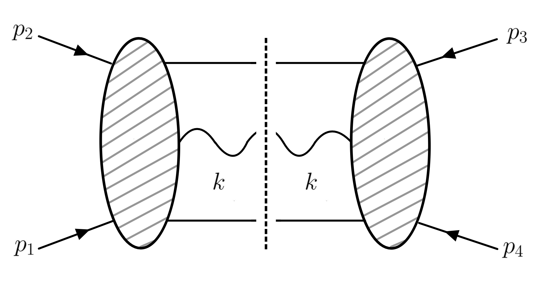
Figure 2: Three-particle cut yielding the infrared divergent part of $\mathrm{Im}\,2\delta_{2}$ in (3.8)

The de Donder projector $P_{\mu\nu;\rho\sigma}=\frac{1}{2}\eta_{\mu\rho}\eta_{\nu\sigma}+\frac{1}{2}\eta_{\mu\sigma}\eta_{\nu\rho}-\frac{1}{2}\eta_{\mu\nu}\eta_{\rho\sigma}$ has been inserted in (3.8) in order to single out only the physical, transverse-traceless projection of $\tilde{\mathcal{A}}_{5}^{\mu\nu}$.

We parametrize the momentum of the emitted graviton as $k=-\omega(1,\hat{\mathbf{x}})$ where $\hat{\mathbf{x}}=(\sin\theta,\sin\theta\sin\varphi,\cos\theta)$ and hence $\left|\mathbf{k}\right|=\omega$. The various scalar product are

$$\mathbf{k}\cdot\mathbf{b}_{\pm}=-\omega\sin\theta[b\cos\varphi\pm(a^{1}\sin\varphi-a^{2}\cos\varphi)],$$ (3.9)

$$\bar{p}_{1}\cdot k=\omega(E_{1}-p\cos\theta),\qquad\bar{p}_{2}\cdot k=\omega(E_{2}+p\cos\theta),$$ (3.10)

$$\mathbf{b}_{\pm}^{2}=b^{2}+(a^{1})^{2}+(a^{2})^{2}\mp 2ba^{2}.$$ (3.11)

where $\mathbf{a}=a^{i}\mathbf{e}_{i}$. Note that the result will not depend on $a^{3}$, component of $\mathbf{a}$ along $\mathbf{p}$. Integrating over $\omega$ and over $\varphi$ and keeping only the term proportional to $\epsilon^{-1}$ we get for the infrared divergent part of the imaginary part of the two-loop eikonal

$$\mathrm{Im}\,2\delta_{2}(\sigma,b) \simeq-\frac{1}{2\epsilon}\frac{\pi}{2\hbar(2\pi)^{3}}\bigg{(}\frac{\kappa^{3}m_{1}m_{2}\sigma^{2}}{8\pi\sqrt{\sigma^{2}-1}}\bigg{)}^{2}\bigg{(}\sum_{\pm}\frac{(1\pm v)^{2}\mathbf{b}_{\pm}}{\mathbf{b}^{2}_{\pm}}\bigg{)}^{2}\mathcal{I}(\sigma),$$ (3.12)

where [82]

$$\mathcal{I}(\sigma)= \int_{-1}^{1}\text{d}x\bigg{\{}\frac{1-x^{2}}{4}\bigg{[}\frac{m_{1}^{4}}{(E_{1}-\bar{p}x)^{4}}+\frac{m_{2}^{4}}{(E_{2}+\bar{p}x)^{4}}-\frac{2m_{1}^{2}m_{2}^{2}(2\sigma^{2}-1)}{(E_{1}-\bar{p}x)^{2}(E_{2}+\bar{p}x)^{2}}\bigg{]}$$

$$-2\bigg{[}\frac{m_{1}^{2}}{(E_{1}-\bar{p}x)^{2}}+\frac{m_{2}^{2}}{(E_{2}+\bar{p}x)^{2}}-\frac{2m_{1}m_{2}\sigma}{(E_{1}-\bar{p}x)(E_{2}+\bar{p}x)}\bigg{]}\bigg{\}}$$

$$=\frac{2}{\sigma^{2}-1}\bigg{[}\frac{8-5\sigma^{2}}{3}-\frac{\sigma(3-2\sigma^{2})}{\sqrt{\sigma^{2}-1}}\cosh^{-1}(\sigma)\bigg{]}.$$ (3.13)

Introducing the notation $\beta(\sigma)=2m_{1}m_{2}G(2\sigma^{2}-1)$ as in [84, 30] and the spatial vector $\mathbf{f}$ as

$$\sum_{\pm}\frac{(1\pm v)^{2}\mathbf{b}_{\pm}}{\mathbf{b}_{\pm}^{2}}\equiv\frac{2(2\sigma^{2}-1)}{\sigma^{2}b}\mathbf{f}(a,b,\sigma),$$ (3.14)

the final result for the infrared divergent part of $\mathrm{Im}\,2\delta_{2}$ can be simply written as

$$\mathrm{Im}\,2\delta_{2}(\sigma,b)\simeq-\frac{1}{2\epsilon}\frac{G\beta^{2}(\sigma)}{2\pi\hbar(\sigma^{2}-1)b^{2}}\mathcal{I}(\sigma)\mathbf{f}^{2}(a,b,\sigma).$$ (3.15)

When the spins are parallel to the orbital angular momentum the vector $\mathbf{f}$ is

$$\mathbf{f}(a,b,\sigma)\equiv f(a,b,\sigma)\frac{\mathbf{b}}{b},\qquad f(a,b,\sigma)=\frac{1+\frac{2\sigma\sqrt{\sigma^{2}-1}}{2\sigma^{2}-1}\frac{a}{b}}{1-\left(\frac{a}{b}\right)^{2}}.$$ (3.16)

For arbitrary spin orientation, $\mathbf{f}$ has non-vanishing components also along $\hat{\mathbf{p}}\times\mathbf{a}$ and explicit expressions for $\mathbf{f}$ and $\mathbf{f}^{2}$ can be found in Appendix A.

Using Eq. (3.1) we can extract the radiative contribution to the real part of the two-loop eikonal

$$\mathrm{Re}\,2\delta_{2}^{\mathrm{rr}}(\sigma,b)=\frac{G\beta^{2}(\sigma)}{4\hbar(\sigma^{2}-1)b^{2}}\mathcal{I}(\sigma)\mathbf{f}^{2}(a,b,\sigma)=\mathrm{Re}\,2\delta_{2}^{\mathrm{rr}}(\sigma,b)\big{|}_{\mathbf{a}=0}\mathbf{f}^{2}(a,b,\sigma),$$ (3.17)

This equation shows that the radiation reaction part of the eikonal of two Kerr black-holes scattering is simply obtained from that of two Schwarzschild black holes by means of a Newman-Janis shift, as stressed after (3.5). In particular, we find a simple rule that allows to get the result for spinning black holes from that of spinless ones. We start to notice that, for the latter, the combination $[2(2\sigma^{2}+1)\mathbf{b}/\sigma^{2}b^{2}]^{2}$ that appears in $\mathrm{Re}\,2\delta_{2}$ can be rewritten as

$$\left(\frac{2(2\sigma^{2}-1)}{\sigma^{2}b^{2}}\mathbf{b}\right)^{2}=\bigg{(}\frac{(1+v)^{2}\mathbf{b}}{\mathbf{b}^{2}}+\frac{(1-v)^{2}\bar{\mathbf{b}}}{\bar{\mathbf{b}}^{2}}\bigg{)}^{2},$$ (3.18)

where we introduced an auxiliary vector $\bar{\mathbf{b}}$ such that $\bar{\mathbf{b}}\stackrel{{\scriptstyle\mathbf{a}=0}}{{=}}\mathbf{b}$. Then to get the result for $\mathbf{a}\neq 0$ we just need to do the replacements

$$\mathbf{b}\stackrel{{\scriptstyle\mathbf{a}\neq 0}}{{\longrightarrow}}\mathbf{b}_{+},\qquad\bar{\mathbf{b}}\stackrel{{\scriptstyle\mathbf{a}\neq 0}}{{\longrightarrow}}\mathbf{b}_{-}.$$ (3.19)

We complete this section by using the first equation of (3.2) for computing the zero frequency limit of the energy spectrum

$$\frac{dE^{\mathrm{rad}}}{d\omega}\bigg{|}_{\omega\to 0}=\frac{4G^{3}m_{1}^{2}m_{2}^{2}(2\sigma^{2}-1)^{2}}{\pi b^{2}(\sigma^{2}-1)}\mathcal{I}(\sigma)\mathbf{f}^{2}(a,b,\sigma),$$ (3.20)

that can be expanded in the static (PN) limit $\sigma\rightarrow 1$ yielding,

$$\frac{dE^{\mathrm{rad}}}{d\omega}\bigg{|}_{\omega\to 0}\simeq\frac{32G^{3}m_{1}^{2}m_{2}^{2}}{5\pi}\frac{b^{2}}{(\mathbf{b}+\hat{\mathbf{p}}\times\mathbf{a})^{2}(\mathbf{b}-\hat{\mathbf{p}}\times\mathbf{a})^{2}},$$ (3.21)

that gives the all orders in spin correction to the original Smarr formula [103, 96]. Further expanding up to quadratic order in spin we find

$$\frac{dE^{\mathrm{rad}}}{d\omega}\bigg{|}_{\omega\to 0}\simeq\frac{32G^{3}m_{1}^{2}m_{2}^{2}}{5\pi b^{2}}\left(1+2\frac{(a^{2})^{2}-(a^{1})^{2}}{b^{2}}\right).$$ (3.22)

When the spins are orthogonal to the scattering plane, Eq. (3.21) reduces to

$$\frac{dE^{\mathrm{rad}}}{d\omega}\bigg{|}_{\omega\to 0}\simeq\frac{32G^{3}m_{1}^{2}m_{2}^{2}}{5\pi b^{2}}\frac{1}{\left[1-\left(\frac{a}{b}\right)^{2}\right]^{2}}.$$ (3.23)

4 Radiative scattering angle and angular momentum loss to all orders in spin

In this section we start studying the case in which the two spins are aligned i.e. we set $a^{1}=0$ and we define $a\equiv a^{2}$ to simplify the notation and from the real part of the eikonal in (3.17) we extract the radiative part of the scattering angle to all orders in spin. In this case the vector $\mathbf{f}$ is given in (3.16) so that the real part of the radiation reaction eikonal becomes

$$\mathrm{Re}\,2\delta_{2}^{\mathrm{rr}}(\sigma,b)=\frac{G\beta^{2}(\sigma)}{4\hbar(\sigma^{2}-1)b^{2}}\mathcal{I}(\sigma)f^{2}(a,b,\sigma),$$ (4.1)

and $\theta^{\mathrm{rr}}_{3}$, using (3.2) is

$$\theta^{\mathrm{rr}}_{3}(\sigma,b)=\frac{G\beta^{2}(\sigma)}{2(\sigma^{2}-1)pb^{3}}\mathcal{I}(\sigma)\frac{(1+\frac{2\sigma\sqrt{\sigma^{2}-1}}{2\sigma^{2}-1}\frac{a}{b})\left[1+\frac{4\sigma\sqrt{\sigma^{2}-1}}{2\sigma^{2}-1}\frac{a}{b}+\left(\frac{a}{b}\right)^{2}\right]}{\left[1-\left(\frac{a}{b}\right)^{2}\right]^{3}}.$$ (4.2)

In the case of spin $1$ that contains only terms up to the order $a^{2}$ the previous expression is equal to

$$\theta^{\mathrm{rr}}_{3}(\sigma,b)=\frac{G\beta^{2}(\sigma)}{2(\sigma^{2}-1)pb^{3}}\mathcal{I}(\sigma)\Bigg{(}1+\frac{6\sigma\sqrt{\sigma^{2}-1}}{2\sigma^{2}-1}\frac{a}{b}+4\frac{6\sigma^{4}-6\sigma^{2}+1}{(2\sigma^{2}-1)^{2}}\frac{a^{2}}{b^{2}}\Bigg{)},$$ (4.3)

that agrees with Eq. (19) of [62] for $s_{E,+}=0$. For spin $1$ the authors of Ref. [62] checked that the deflection angle is not divergent at high energy because the logarithmic divergence that one finds in the conservative part is cancelled by the logarithmic divergence appearing in the radiative part in analogy with what happens for spin zero. Assuming that the same cancellation also happens for arbitrary spin, from the high energy behaviour of the real part of the two-loop eikonal given by

$$\mathrm{Re}\,2\delta_{2}^{\mathrm{rr}}(\sigma,b)\sim\frac{16G^{3}m_{1}^{2}m_{2}^{2}}{(1-\frac{a}{b})^{2}}\sigma^{2}\log\sigma,\qquad\sigma\to\infty,$$ (4.4)

we can deduce the high energy limit of the conservative part of the real part of the two-loop eikonal

$$\mathrm{Re}\,2\delta_{2}^{\mathrm{cons}}(\sigma,b)\sim-\frac{16G^{3}m_{1}^{2}m_{2}^{2}}{(1-\frac{a}{b})^{2}}\sigma^{2}\log\sigma,\qquad\sigma\to\infty.$$ (4.5)

This implies that the high energy limit of the conservative scattering angle must be equal to

$$\theta^{\mathrm{cons}}_{3}(\sigma,b)\simeq-\frac{32G^{3}Em_{1}m_{2}}{(1-\frac{a}{b})^{3}}\sigma\log\sigma,\qquad\sigma\to\infty,$$ (4.6)

The previous equations are valid for any spin and in particular Eq. (4.6) agrees with the high energy limit of Eqs. (16a), (16b) and (16c) of Ref. [62].

Then we want to use Eq. (3.3) to determine the 2PM loss of angular momentum from the radiative scattering angle. To do so we need the 1PM conservative scattering angle $\theta_{1}^{\mathrm{cons}}$ [37, 41]

$$\theta_{1}^{\mathrm{cons}}(\sigma,b)=\frac{\beta(\sigma)}{pb\sqrt{\sigma^{2}-1}}f(a,b,\sigma)=\frac{\beta(\sigma)}{J\sqrt{\sigma^{2}-1}}\left(\frac{1+\frac{2\sqrt{\sigma^{2}-1}}{2\sigma^{2}-1}\frac{pa}{J}}{1-\left(\frac{pa}{J}\right)^{2}}\right).$$ (4.7)

that is given by $-\frac{1}{p}\frac{\partial\chi_{1}}{\partial b}$, where $\chi_{1}$ is the 1PM eikonal, obtained by inserting the tree-level $4$-point amplitude of (2.1) in Eq. (3.5).

We find that the 2PM loss of angular momentum in the center-of-mass frame is equal to

$$\mathbf{J}^{\mathrm{loss}}_{2}(\sigma,b)=J\frac{G\beta(\sigma)}{b^{2}\sqrt{\sigma^{2}-1}}\mathcal{I}(\sigma)\hat{\mathbf{p}}\times\left(f(a,b,\sigma)\frac{\mathbf{b}}{b}\right)=J\frac{G\beta(\sigma)}{b^{2}\sqrt{\sigma^{2}-1}}\mathcal{I}(\sigma)f(a,b,\sigma)\mathbf{e}_{2}.$$ (4.8)

Note that the only non-vanishing component of the 2PM angular momentum loss is along the $\mathbf{e}_{2}$ direction, perpendicular to the scattering plane. This is due to the fact that in the aligned-spin case the scattering dynamics is planar, just as in the spinless scenario.

We note that (4.8) admits a natural generalisation in the case of non-aligned spin as

$$\mathbf{J}^{\mathrm{loss}}_{2}(\sigma,b)=J\frac{G\beta(\sigma)}{b^{2}\sqrt{\sigma^{2}-1}}\mathcal{I}(\sigma)\hat{\mathbf{p}}\times\mathbf{f}(a,b,\sigma).$$ (4.9)

Contrarily to (3.16), in this case $\mathbf{f}$ does not lie entirely along $\mathbf{b}$, but has also one non-vanishing component along $\hat{\mathbf{p}}\times\mathbf{a}$, see Appendix A. Therefore, as already mentioned, the 2PM angular momentum loss in the center-of-mass frame has components in both directions orthogonal to $\hat{\mathbf{p}}$. Even if (4.9) has been obtained by generalising (4.8) straightforwardly, it admits an interpretation as follows. Introducing the 1PM classical momentum transfer as $Q^{\mu}_{1}=-\frac{\partial\chi_{1}}{\partial b_{\mu}}$, we find $Q^{0}_{1}=0$ and

$$\mathbf{Q}_{1}(\sigma,b)=\frac{\beta(\sigma)}{b\sqrt{\sigma^{2}-1}}\mathbf{f}(a,b,\sigma),\qquad\hat{\mathbf{p}}\cdot\mathbf{Q}_{1}=0,$$ (4.10)

so that (4.9) can be more conveniently rewritten as

$$\mathbf{J}_{2}^{\mathrm{loss}}(\sigma,b)=G\,\mathcal{I}(\sigma)\,\mathbf{p}\times\mathbf{Q}_{1}(\sigma,b)=\mathbf{L}_{2}^{\mathrm{loss}}(\sigma,b)+\mathbf{S}_{2}^{\mathrm{loss}}(\sigma,b),$$ (4.11)

where

$$\mathbf{L}^{\mathrm{loss}}_{2}=G\,\mathcal{I}(\sigma)c_{o}(a,b,\sigma)\mathbf{p}\times\mathbf{b}\qquad\mathbf{S}^{\mathrm{loss}}_{2}(a,b,\sigma)=G\,\mathcal{I}(\sigma)c_{s}(a,b,\sigma)\mathbf{a},$$ (4.12)

where $c_{o}$ and $c_{s}$ have been defined in Appendix A. The 2PM angular momentum loss receives contributions from the variation of directions of the momenta and of the spin vectors of the particles involved in the scattering process.
Expanding equations (4.8) and (4.9) up to quadratic order in the spin we find respectively

$$\mathbf{J}^{\mathrm{loss}}_{2}(\sigma,b)=J\frac{G\beta(\sigma)}{b^{2}\sqrt{\sigma^{2}-1}}\mathcal{I}(\sigma)\left[1+\frac{2\sigma\sqrt{\sigma^{2}-1}}{2\sigma^{2}-1}\frac{a}{b}+\left(\frac{a}{b}\right)^{2}\right]\mathbf{e}_{2},$$ (4.13)

for aligned spins and

$$\mathbf{J}^{\mathrm{loss}}_{2}(\sigma,b) =J\frac{G\beta(\sigma)}{b^{2}\sqrt{\sigma^{2}-1}}\mathcal{I}(\sigma)\left[\bigg{(}-\frac{2\sigma\sqrt{\sigma^{2}-1}}{2\sigma^{2}-1}\frac{a^{1}}{b}-2\frac{a^{1}a^{2}}{b^{2}}\bigg{)}\mathbf{e}_{1}\right.$$

$$+\left.\bigg{(}1+\frac{2\sigma\sqrt{\sigma^{2}-1}}{2\sigma^{2}-1}\frac{a^{2}}{b}+\frac{(a^{2})^{2}-(a^{1})^{2}}{b^{2}}\bigg{)}\mathbf{e}_{2},\right],$$ (4.14)

for non-aligned spins. These equations exactly match equation (18) of [62] and equation (29) of [55] obtained with supersymmetric worldline formalism. Note that equation (4.2), (4.8) and (4.9) extend these results to all orders in spin.

5 Conclusions and outlook

From the leading soft term of a five-point amplitude involving two particles with spin minimally coupled to gravity that scatter producing also a low-energy graviton, we have computed the infrared divergent piece of the imaginary part of the two-loop eikonal, $\delta_{2}$, generalising the procedure followed for spin zero in Ref. [84]. Using then analyticity and crossing symmetry [84] we have derived the radiation reaction contribution to the real part of the $\delta_{2}$ and from it the radiation reaction contribution to the deflection angle at 3PM ($\mathcal{O}(G^{3})$).

Using the Bini-Damour relation in Eq. (3.3), we have determined the angular momentum loss at $\mathcal{O}(G^{2})$ for arbitrary spin configurations and to all orders in spin.

Our results agree for spin zero with those in Refs. [82, 84] and for spin one with the complete calculation performed in Ref. [62].

An interesting aspect of our results is that spin effects for soft bremsstrahlung are entirely encoded in the vector $\mathbf{f}$ in (3.14), that comes from a Newman-Janis shift in impact parameter space, as explained in (3.19). The origin of this unexpected feature is that the entire calculation we have performed has the tree-level four-point amplitude in (2.1) as starting point. In the latter, the spin structure appears as compactly organised in a single exponential factor, because of the nature of minimally coupled amplitudes. It would be interesting to understand to what extent such a simple criterion could be used to gather additional information about the conservative part of $\delta_{2}$, whose ultra-relativistic behaviour appears to be already fixed by the present analysis.

In equation (3.20) we have shown the zero frequency limit of the emitted energy spectrum at $\mathcal{O}(G^{3})$. The reason why we could do this is that we have only used the Weinberg’s soft graviton theorem to determine the leading term of the inelastic five-point amplitude, because it was the necessary ingredient to fix the infrared divergence in $\mathrm{Im}\,2\delta_{2}$. In principle, one could go further in the soft expansion [93, 94], therefore considering also terms containing the total angular momentum operator, and understand how they contribute to the emitted energy and angular momentum spectrum beyond the leading soft limit.

Acknowledgements

We thank Luca Buoninfante, Alessandro Georgoudis, Kays Haddad, Carlo Heissenberg, Henrik Johansson, Alexander Ochirov, Paolo Pichini, Rodolfo Russo, Ali Seraj and Justin Vines for many very useful discussions. We thank Gabriele Veneziano for a critical reading of the first version of our paper. The research of FA (PDV) is fully (partially) supported by the Knut and Alice Wallenberg Foundation under grant KAW 2018.0116. Nordita is partially supported by Nordforsk.

Appendix A Expressions for $\mathbf{f}(a,b,\sigma)$

The vector $\mathbf{f}$ introduced in (3.14) can be written as

$$\mathbf{f}(a,b,\sigma)=c_{o}(a,b,\sigma)\mathbf{b}-c_{s}(a,b,\sigma)\hat{\mathbf{p}}\times\mathbf{a},$$ (A.1)

where

$$c_{o}(a,b,\sigma)=\frac{b[(\sigma+\sqrt{\sigma^{2}-1})^{2}\left|\mathbf{b}-\hat{\mathbf{p}}\times\mathbf{a}\right|^{2}+(\sigma-\sqrt{\sigma^{2}-1})^{2}\left|\mathbf{b}+\hat{\mathbf{p}}\times\mathbf{a}\right|^{2}]}{2(2\sigma^{2}-1)\left|\mathbf{b}-\hat{\mathbf{p}}\times\mathbf{a}\right|^{2}\left|\mathbf{b}+\hat{\mathbf{p}}\times\mathbf{a}\right|^{2}},$$ (A.2)

$$c_{s}(a,b,\sigma)=\frac{(\sigma-\sqrt{\sigma^{2}-1})^{2}\left|\mathbf{b}+\hat{\mathbf{p}}\times\mathbf{a}\right|^{2}]-b[(\sigma+\sqrt{\sigma^{2}-1})^{2}\left|\mathbf{b}-\hat{\mathbf{p}}\times\mathbf{a}\right|^{2}}{2(2\sigma^{2}-1)\left|\mathbf{b}-\hat{\mathbf{p}}\times\mathbf{a}\right|^{2}\left|\mathbf{b}+\hat{\mathbf{p}}\times\mathbf{a}\right|^{2}}.$$ (A.3)

The components of $\mathbf{f}$ are explicitly given by

$$f^{1}(a,b,\sigma)=\frac{\left(1+\frac{(a^{1})^{2}+(a^{2})^{2}}{b^{2}}\right)\left(1-\frac{2\sigma\sqrt{\sigma^{2}-1}}{2\sigma^{2}-1}\frac{a^{2}}{b}\right)+\frac{2a^{2}}{b}\left(\frac{2\sigma\sqrt{\sigma^{2}-1}}{2\sigma^{2}-1}-\frac{a^{2}}{b}\right)}{(1-\frac{2a^{2}}{b}+\frac{(a^{1})^{2}+(a^{2})^{2}}{b^{2}})(1+\frac{2a^{2}}{b}+\frac{(a^{1})^{2}+(a^{2})^{2}}{b^{2}})},$$ (A.4)

$$f^{2}(a,b,\sigma)=\frac{\frac{2\sigma\sqrt{\sigma^{2}-1}}{2\sigma^{2}-1}\frac{a^{1}}{b}\left(1+\frac{2\sigma^{2}-1}{\sigma\sqrt{\sigma^{2}-1}}\frac{a^{2}}{b}+\frac{(a^{1})^{2}+(a^{2})^{2}}{b^{2}}\right)}{(1-\frac{2a^{2}}{b}+\frac{(a^{1})^{2}+(a^{2})^{2}}{b^{2}})(1+\frac{2a^{2}}{b}+\frac{(a^{1})^{2}+(a^{2})^{2}}{b^{2}})},$$ (A.5)

$$f^{3}(a,b,\sigma)=0.$$ (A.6)

Therefore we have

$$\mathbf{f}^{2}(a,b,\sigma)=\frac{1+\frac{4\sigma\sqrt{\sigma^{2}-1}}{2\sigma^{2}-1}\frac{a^{2}}{b}+\frac{4\sigma^{2}(\sigma^{2}-1)}{(2\sigma^{2}-1)^{2}}\frac{(a^{1})^{2}+(a^{2})^{2}}{b^{2}}}{(1-\frac{2a^{2}}{b}+\frac{(a^{1})^{2}+(a^{2})^{2}}{b^{2}})(1+\frac{2a^{2}}{b}+\frac{(a^{1})^{2}+(a^{2})^{2}}{b^{2}})}.$$ (A.7)

References

- [1] LIGO Scientific, Virgo Collaboration, B. P. Abbott et al., “Observation of Gravitational Waves from a Binary Black Hole Merger,” Phys. Rev. Lett. 116 no. 6, (2016) 061102, arXiv:1602.03837 [gr-qc].
- [2] LIGO Scientific, Virgo Collaboration, B. P. Abbott et al., “GW151226: Observation of Gravitational Waves from a 22-Solar-Mass Binary Black Hole Coalescence,” Phys. Rev. Lett. 116 no. 24, (2016) 241103, arXiv:1606.04855 [gr-qc].
- [3] LIGO Scientific, VIRGO Collaboration, B. P. Abbott et al., “GW170104: Observation of a 50-Solar-Mass Binary Black Hole Coalescence at Redshift 0.2,” Phys. Rev. Lett. 118 no. 22, (2017) 221101, arXiv:1706.01812 [gr-qc]. [Erratum: Phys.Rev.Lett. 121, 129901 (2018)].
- [4] LIGO Scientific, Virgo Collaboration, B. P. Abbott et al., “GW170814: A Three-Detector Observation of Gravitational Waves from a Binary Black Hole Coalescence,” Phys. Rev. Lett. 119 no. 14, (2017) 141101, arXiv:1709.09660 [gr-qc].
- [5] LIGO Scientific, Virgo Collaboration, B. P. Abbott et al., “GW170817: Observation of Gravitational Waves from a Binary Neutron Star Inspiral,” Phys. Rev. Lett. 119 no. 16, (2017) 161101, arXiv:1710.05832 [gr-qc].
- [6] LIGO Scientific, Virgo Collaboration, B. P. Abbott et al., “GWTC-1: A Gravitational-Wave Transient Catalog of Compact Binary Mergers Observed by LIGO and Virgo during the First and Second Observing Runs,” Phys. Rev. X 9 no. 3, (2019) 031040, arXiv:1811.12907 [astro-ph.HE].
- [7] LIGO Scientific, Virgo Collaboration, R. Abbott et al., “GWTC-2: Compact Binary Coalescences Observed by LIGO and Virgo During the First Half of the Third Observing Run,” Phys. Rev. X 11 (2021) 021053, arXiv:2010.14527 [gr-qc].
- [8] A. Buonanno and T. Damour, “Effective one-body approach to general relativistic two-body dynamics,” Phys. Rev. D59 (1999) 084006, arXiv:gr-qc/9811091 [gr-qc].
- [9] W. D. Goldberger and I. Z. Rothstein, “An Effective field theory of gravity for extended objects,” Phys. Rev. D 73 (2006) 104029, arXiv:hep-th/0409156.
- [10] W. D. Goldberger and A. K. Ridgway, “Radiation and the classical double copy for color charges,” Phys. Rev. D 95 no. 12, (2017) 125010, arXiv:1611.03493 [hep-th].
- [11] A. Luna, I. Nicholson, D. O’Connell, and C. D. White, “Inelastic Black Hole Scattering from Charged Scalar Amplitudes,” JHEP 03 (2018) 044, arXiv:1711.03901 [hep-th].
- [12] C. Cheung, I. Z. Rothstein, and M. P. Solon, “From Scattering Amplitudes to Classical Potentials in the Post-Minkowskian Expansion,” Phys. Rev. Lett. 121 no. 25, (2018) 251101, arXiv:1808.02489 [hep-th].
- [13] D. A. Kosower, B. Maybee, and D. O’Connell, “Amplitudes, Observables, and Classical Scattering,” JHEP 02 (2019) 137, arXiv:1811.10950 [hep-th].
- [14] N. E. J. Bjerrum-Bohr, P. H. Damgaard, G. Festuccia, L. Planté, and P. Vanhove, “General Relativity from Scattering Amplitudes,” Phys. Rev. Lett. 121 no. 17, (2018) 171601, arXiv:1806.04920 [hep-th].
- [15] N. Bjerrum-Bohr, A. Cristofoli, and P. H. Damgaard, “Post-Minkowskian Scattering Angle in Einstein Gravity,” JHEP 08 (2020) 038, arXiv:1910.09366 [hep-th].
- [16] G. Kälin and R. A. Porto, “From Boundary Data to Bound States,” JHEP 01 (2020) 072, arXiv:1910.03008 [hep-th].
- [17] G. Kälin and R. A. Porto, “From boundary data to bound states. Part II. Scattering angle to dynamical invariants (with twist),” JHEP 02 (2020) 120, arXiv:1911.09130 [hep-th].
- [18] G. Cho, G. Kälin, and R. A. Porto, “From Boundary Data to Bound States III: Radiative Effects,” arXiv:2112.03976 [hep-th].
- [19] A. Cristofoli, P. H. Damgaard, P. Di Vecchia, and C. Heissenberg, “Second-order Post-Minkowskian scattering in arbitrary dimensions,” JHEP 07 (2020) 122, arXiv:2003.10274 [hep-th].
- [20] G. Mogull, J. Plefka, and J. Steinhoff, “Classical black hole scattering from a worldline quantum field theory,” JHEP 02 (2021) 048, arXiv:2010.02865 [hep-th].
- [21] M. Accettulli Huber, A. Brandhuber, S. De Angelis, and G. Travaglini, “From amplitudes to gravitational radiation with cubic interactions and tidal effects,” Phys. Rev. D 103 no. 4, (2021) 045015, arXiv:2012.06548 [hep-th].
- [22] L. de la Cruz, B. Maybee, D. O’Connell, and A. Ross, “Classical Yang-Mills observables from amplitudes,” JHEP 12 (2020) 076, arXiv:2009.03842 [hep-th].
- [23] A. Cristofoli, R. Gonzo, D. A. Kosower, and D. O’Connell, “Waveforms from Amplitudes,” arXiv:2107.10193 [hep-th].
- [24] E. Herrmann, J. Parra-Martinez, M. S. Ruf, and M. Zeng, “Radiative classical gravitational observables at (G3) from scattering amplitudes,” JHEP 10 (2021) 148, arXiv:2104.03957 [hep-th].
- [25] A. Cristofoli, R. Gonzo, N. Moynihan, D. O’Connell, A. Ross, M. Sergola, and C. D. White, “The Uncertainty Principle and Classical Amplitudes,” arXiv:2112.07556 [hep-th].
- [26] T. Damour, “High-energy gravitational scattering and the general relativistic two-body problem,” Phys. Rev. D97 no. 4, (2018) 044038, arXiv:1710.10599 [gr-qc].
- [27] S. Mougiakakos, M. M. Riva, and F. Vernizzi, “Gravitational Bremsstrahlung in the Post-Minkowskian Effective Field Theory,” arXiv:2102.08339 [gr-qc].
- [28] G. U. Jakobsen, G. Mogull, J. Plefka, and J. Steinhoff, “Classical Gravitational Bremsstrahlung from a Worldline Quantum Field Theory,” arXiv:2101.12688 [gr-qc].
- [29] E. Herrmann, J. Parra-Martinez, M. S. Ruf, and M. Zeng, “Gravitational Bremsstrahlung from Reverse Unitarity,” arXiv:2101.07255 [hep-th].
- [30] P. Di Vecchia, C. Heissenberg, R. Russo, and G. Veneziano, “The eikonal approach to gravitational scattering and radiation at (G3),” JHEP 07 (2021) 169, arXiv:2104.03256 [hep-th].
- [31] N. Arkani-Hamed, T.-C. Huang, and Y.-t. Huang, “Scattering amplitudes for all masses and spins,” JHEP 11 (2021) 070, arXiv:1709.04891 [hep-th].
- [32] A. Guevara, “Holomorphic Classical Limit for Spin Effects in Gravitational and Electromagnetic Scattering,” JHEP 04 (2019) 033, arXiv:1706.02314 [hep-th].
- [33] D. Bini and T. Damour, “Gravitational spin-orbit coupling in binary systems, post-Minkowskian approximation and effective one-body theory,” Phys. Rev. D 96 no. 10, (2017) 104038, arXiv:1709.00590 [gr-qc].
- [34] J. Vines, “Scattering of two spinning black holes in post-Minkowskian gravity, to all orders in spin, and effective-one-body mappings,” Class. Quant. Grav. 35 no. 8, (2018) 084002, arXiv:1709.06016 [gr-qc].
- [35] D. Bini and T. Damour, “Gravitational spin-orbit coupling in binary systems at the second post-Minkowskian approximation,” Phys. Rev. D 98 no. 4, (2018) 044036, arXiv:1805.10809 [gr-qc].
- [36] J. Vines, J. Steinhoff, and A. Buonanno, “Spinning-black-hole scattering and the test-black-hole limit at second post-Minkowskian order,” Phys. Rev. D 99 no. 6, (2019) 064054, arXiv:1812.00956 [gr-qc].
- [37] A. Guevara, A. Ochirov, and J. Vines, “Scattering of Spinning Black Holes from Exponentiated Soft Factors,” JHEP 09 (2019) 056, arXiv:1812.06895 [hep-th].
- [38] M.-Z. Chung, Y.-T. Huang, J.-W. Kim, and S. Lee, “The simplest massive S-matrix: from minimal coupling to Black Holes,” JHEP 04 (2019) 156, arXiv:1812.08752 [hep-th].
- [39] Y. F. Bautista and A. Guevara, “From Scattering Amplitudes to Classical Physics: Universality, Double Copy and Soft Theorems,” arXiv:1903.12419 [hep-th].
- [40] B. Maybee, D. O’Connell, and J. Vines, “Observables and amplitudes for spinning particles and black holes,” JHEP 12 (2019) 156, arXiv:1906.09260 [hep-th].
- [41] A. Guevara, A. Ochirov, and J. Vines, “Black-hole scattering with general spin directions from minimal-coupling amplitudes,” Phys. Rev. D 100 no. 10, (2019) 104024, arXiv:1906.10071 [hep-th].
- [42] N. Arkani-Hamed, Y.-t. Huang, and D. O’Connell, “Kerr black holes as elementary particles,” JHEP 01 (2020) 046, arXiv:1906.10100 [hep-th].
- [43] H. Johansson and A. Ochirov, “Double copy for massive quantum particles with spin,” JHEP 09 (2019) 040, arXiv:1906.12292 [hep-th].
- [44] M.-Z. Chung, Y.-T. Huang, and J.-W. Kim, “Classical potential for general spinning bodies,” JHEP 09 (2020) 074, arXiv:1908.08463 [hep-th].
- [45] P. H. Damgaard, K. Haddad, and A. Helset, “Heavy Black Hole Effective Theory,” JHEP 11 (2019) 070, arXiv:1908.10308 [hep-ph].
- [46] Y. F. Bautista and A. Guevara, “On the double copy for spinning matter,” JHEP 11 (2021) 184, arXiv:1908.11349 [hep-th].
- [47] R. Aoude, K. Haddad, and A. Helset, “On-shell heavy particle effective theories,” JHEP 05 (2020) 051, arXiv:2001.09164 [hep-th].
- [48] M.-Z. Chung, Y.-t. Huang, J.-W. Kim, and S. Lee, “Complete Hamiltonian for spinning binary systems at first post-Minkowskian order,” JHEP 05 (2020) 105, arXiv:2003.06600 [hep-th].
- [49] Z. Bern, A. Luna, R. Roiban, C.-H. Shen, and M. Zeng, “Spinning black hole binary dynamics, scattering amplitudes, and effective field theory,” Phys. Rev. D 104 no. 6, (2021) 065014, arXiv:2005.03071 [hep-th].
- [50] R. Aoude, K. Haddad, and A. Helset, “Tidal effects for spinning particles,” JHEP 03 (2021) 097, arXiv:2012.05256 [hep-th].
- [51] A. Guevara, B. Maybee, A. Ochirov, D. O’connell, and J. Vines, “A worldsheet for Kerr,” JHEP 03 (2021) 201, arXiv:2012.11570 [hep-th].
- [52] Z. Liu, R. A. Porto, and Z. Yang, “Spin Effects in the Effective Field Theory Approach to Post-Minkowskian Conservative Dynamics,” JHEP 06 (2021) 012, arXiv:2102.10059 [hep-th].
- [53] D. Kosmopoulos and A. Luna, “Quadratic-in-spin Hamiltonian at (G2) from scattering amplitudes,” JHEP 07 (2021) 037, arXiv:2102.10137 [hep-th].
- [54] R. Aoude and A. Ochirov, “Classical observables from coherent-spin amplitudes,” JHEP 10 (2021) 008, arXiv:2108.01649 [hep-th].
- [55] G. U. Jakobsen, G. Mogull, J. Plefka, and J. Steinhoff, “Gravitational Bremsstrahlung and Hidden Supersymmetry of Spinning Bodies,” Phys. Rev. Lett. 128 no. 1, (2022) 011101, arXiv:2106.10256 [hep-th].
- [56] Y. F. Bautista, A. Guevara, C. Kavanagh, and J. Vines, “From Scattering in Black Hole Backgrounds to Higher-Spin Amplitudes: Part I,” arXiv:2107.10179 [hep-th].
- [57] M. Chiodaroli, H. Johansson, and P. Pichini, “Compton black-hole scattering for s 5/2,” JHEP 02 (2022) 156, arXiv:2107.14779 [hep-th].
- [58] K. Haddad, “Exponentiation of the leading eikonal phase with spin,” Phys. Rev. D 105 no. 2, (2022) 026004, arXiv:2109.04427 [hep-th].
- [59] G. U. Jakobsen, G. Mogull, J. Plefka, and J. Steinhoff, “SUSY in the sky with gravitons,” JHEP 01 (2022) 027, arXiv:2109.04465 [hep-th].
- [60] M. V. S. Saketh, J. Vines, J. Steinhoff, and A. Buonanno, “Conservative and radiative dynamics in classical relativistic scattering and bound systems,” Phys. Rev. Res. 4 no. 1, (2022) 013127, arXiv:2109.05994 [gr-qc].
- [61] W.-M. Chen, M.-Z. Chung, Y.-t. Huang, and J.-W. Kim, “The 2PM Hamiltonian for binary Kerr to quartic in spin,” arXiv:2111.13639 [hep-th].
- [62] G. U. Jakobsen and G. Mogull, “Conservative and radiative dynamics of spinning bodies at third post-Minkowskian order using worldline quantum field theory,” arXiv:2201.07778 [hep-th].
- [63] R. Aoude, K. Haddad, and A. Helset, “Searching for Kerr in the 2PM amplitude,” arXiv:2203.06197 [hep-th].
- [64] Z. Bern, D. Kosmopoulos, A. Luna, R. Roiban, and F. Teng, “Binary Dynamics Through the Fifth Power of Spin at ,” arXiv:2203.06202 [hep-th].
- [65] T. Adamo, A. Cristofoli, and P. Tourkine, “Eikonal amplitudes from curved backgrounds,” arXiv:2112.09113 [hep-th].
- [66] L. Blanchet, “Gravitational radiation from post-Newtonian sources and inspiralling compact binaries,” Living Rev. Rel. 9 (2006) 4.
- [67] M. Levi and J. Steinhoff, “Equivalence of ADM Hamiltonian and Effective Field Theory approaches at next-to-next-to-leading order spin1-spin2 coupling of binary inspirals,” JCAP 12 (2014) 003, arXiv:1408.5762 [gr-qc].
- [68] M. Levi and J. Steinhoff, “Spinning gravitating objects in the effective field theory in the post-Newtonian scheme,” JHEP 09 (2015) 219, arXiv:1501.04956 [gr-qc].
- [69] M. Levi and J. Steinhoff, “Next-to-next-to-leading order gravitational spin-orbit coupling via the effective field theory for spinning objects in the post-Newtonian scheme,” JCAP 01 (2016) 011, arXiv:1506.05056 [gr-qc].
- [70] M. Levi and J. Steinhoff, “Next-to-next-to-leading order gravitational spin-squared potential via the effective field theory for spinning objects in the post-Newtonian scheme,” JCAP 01 (2016) 008, arXiv:1506.05794 [gr-qc].
- [71] M. Levi and J. Steinhoff, “Complete conservative dynamics for inspiralling compact binaries with spins at the fourth post-Newtonian order,” JCAP 09 (2021) 029, arXiv:1607.04252 [gr-qc].
- [72] M. Levi, S. Mougiakakos, and M. Vieira, “Gravitational cubic-in-spin interaction at the next-to-leading post-Newtonian order,” JHEP 01 (2021) 036, arXiv:1912.06276 [hep-th].
- [73] M. Levi and F. Teng, “NLO gravitational quartic-in-spin interaction,” JHEP 01 (2021) 066, arXiv:2008.12280 [hep-th].
- [74] M. Levi, A. J. Mcleod, and M. Von Hippel, “N3LO gravitational spin-orbit coupling at order ,” JHEP 07 (2021) 115, arXiv:2003.02827 [hep-th].
- [75] M. Levi, A. J. Mcleod, and M. Von Hippel, “N3LO gravitational quadratic-in-spin interactions at G4,” JHEP 07 (2021) 116, arXiv:2003.07890 [hep-th].
- [76] J.-W. Kim, M. Levi, and Z. Yin, “Quadratic-in-spin interactions at fifth post-Newtonian order probe new physics,” arXiv:2112.01509 [hep-th].
- [77] P. Di Vecchia, C. Heissenberg, R. Russo, and G. Veneziano, “Universality of ultra-relativistic gravitational scattering,” Phys. Lett. B 811 (2020) 135924, arXiv:2008.12743 [hep-th].
- [78] Z. Bern, C. Cheung, R. Roiban, C.-H. Shen, M. P. Solon, and M. Zeng, “Scattering Amplitudes and the Conservative Hamiltonian for Binary Systems at Third Post-Minkowskian Order,” Phys. Rev. Lett. 122 no. 20, (2019) 201603, arXiv:1901.04424 [hep-th].
- [79] Z. Bern, C. Cheung, R. Roiban, C.-H. Shen, M. P. Solon, and M. Zeng, “Black Hole Binary Dynamics from the Double Copy and Effective Theory,” JHEP 10 (2019) 206, arXiv:1908.01493 [hep-th].
- [80] G. Kälin, Z. Liu, and R. A. Porto, “Conservative Dynamics of Binary Systems to Third Post-Minkowskian Order from the Effective Field Theory Approach,” Phys. Rev. Lett. 125 no. 26, (2020) 261103, arXiv:2007.04977 [hep-th].
- [81] J. Parra-Martinez, M. S. Ruf, and M. Zeng, “Extremal black hole scattering at : graviton dominance, eikonal exponentiation, and differential equations,” JHEP 11 (2020) 023, arXiv:2005.04236 [hep-th].
- [82] T. Damour, “Radiative contribution to classical gravitational scattering at the third order in ,” Phys. Rev. D 102 no. 12, (2020) 124008, arXiv:2010.01641 [gr-qc].
- [83] D. Bini and T. Damour, “Gravitational radiation reaction along general orbits in the effective one-body formalism,” Phys. Rev. D 86 (2012) 124012, arXiv:1210.2834 [gr-qc].
- [84] P. Di Vecchia, C. Heissenberg, R. Russo, and G. Veneziano, “Radiation Reaction from Soft Theorems,” Phys. Lett. B 818 (2021) 136379, arXiv:2101.05772 [hep-th].
- [85] D. Amati, M. Ciafaloni, and G. Veneziano, “Higher Order Gravitational Deflection and Soft Bremsstrahlung in Planckian Energy Superstring Collisions,” Nucl. Phys. B 347 (1990) 550–580.
- [86] N. E. J. Bjerrum-Bohr, P. H. Damgaard, L. Planté, and P. Vanhove, “Classical gravity from loop amplitudes,” Phys. Rev. D 104 no. 2, (2021) 026009, arXiv:2104.04510 [hep-th].
- [87] N. E. J. Bjerrum-Bohr, P. H. Damgaard, L. Planté, and P. Vanhove, “The amplitude for classical gravitational scattering at third Post-Minkowskian order,” JHEP 08 (2021) 172, arXiv:2105.05218 [hep-th].
- [88] A. Brandhuber, G. Chen, G. Travaglini, and C. Wen, “Classical gravitational scattering from a gauge-invariant double copy,” JHEP 10 (2021) 118, arXiv:2108.04216 [hep-th].
- [89] D. Bini, T. Damour, and A. Geralico, “Radiative contributions to gravitational scattering,” Phys. Rev. D 104 no. 8, (2021) 084031, arXiv:2107.08896 [gr-qc].
- [90] P. Di Vecchia, C. Heissenberg, and R. Russo, “Angular momentum of zero-frequency gravitons,” arXiv:2203.11915 [hep-th].
- [91] E. T. Newman and A. I. Janis, “Note on the Kerr spinning particle metric,” J. Math. Phys. 6 (1965) 915–917.
- [92] S. Weinberg, “Infrared photons and gravitons,” Phys. Rev. 140 (1965) B516–B524.
- [93] F. Cachazo and A. Strominger, “Evidence for a New Soft Graviton Theorem,” arXiv:1404.4091 [hep-th].
- [94] Z. Bern, S. Davies, P. Di Vecchia, and J. Nohle, “Low-Energy Behavior of Gluons and Gravitons from Gauge Invariance,” Phys. Rev. D 90 no. 8, (2014) 084035, arXiv:1406.6987 [hep-th].
- [95] C. Heissenberg, “Infrared divergences and the eikonal exponentiation,” Phys. Rev. D 104 no. 4, (2021) 046016, arXiv:2105.04594 [hep-th].
- [96] L. Smarr, “Gravitational Radiation from Distant Encounters and from Headon Collisions of Black Holes: The Zero Frequency Limit,” Phys. Rev. D 15 (1977) 2069–2077.
- [97] G. Veneziano and G. A. Vilkovisky, “Angular momentum loss in gravitational scattering, radiation reaction, and the Bondi gauge ambiguity,” arXiv:2201.11607 [gr-qc].
- [98] A. V. Manohar, A. K. Ridgway, and C.-H. Shen, “Radiated Angular Momentum and Dissipative Effects in Classical Scattering,” arXiv:2203.04283 [hep-th].
- [99] R. Monteiro, S. Nagy, D. O’Connell, D. Peinador Veiga, and M. Sergola, “NS-NS Spacetimes from Amplitudes,” arXiv:2112.08336 [hep-th].
- [100] R. Monteiro, D. O’Connell, and C. D. White, “Black holes and the double copy,” JHEP 12 (2014) 056, arXiv:1410.0239 [hep-th].
- [101] A. Luna, R. Monteiro, I. Nicholson, D. O’Connell, and C. D. White, “The double copy: Bremsstrahlung and accelerating black holes,” JHEP 06 (2016) 023, arXiv:1603.05737 [hep-th].
- [102] D. Amati, M. Ciafaloni, and G. Veneziano, “Towards an S-matrix description of gravitational collapse,” JHEP 02 (2008) 049, arXiv:0712.1209 [hep-th].
- [103] R. Ruffini and J. A. Wheeler, “RELATIVISTIC COSMOLOGY AND SPACE PLATFORMS,” 8, 1970.