Shoring Up the Foundations:
Fusing Model Embeddings and Weak Supervision

Abstract

Foundation models offer an exciting new paradigm for constructing models with out-of-the-box embeddings and a few labeled examples. However, it is not clear how to best apply foundation models without labeled data. A potential approach is to fuse foundation models with weak supervision frameworks, which use weak label sources—pre-trained models, heuristics, crowd-workers—to construct pseudolabels. The challenge is building a combination that best exploits the signal available in both foundation models and weak sources. We propose Liger, a combination that uses foundation model embeddings to improve two crucial elements of existing weak supervision techniques. First, we produce finer estimates of weak source quality by partitioning the embedding space and learning per-part source accuracies. Second, we improve source coverage by extending source votes in embedding space. Despite the black-box nature of foundation models, we prove results characterizing how our approach improves performance and show that lift scales with the smoothness of label distributions in embedding space. On six benchmark NLP and video tasks, Liger outperforms vanilla weak supervision by 14.1 points, weakly-supervised kNN and adapters by 11.8 points, and kNN and adapters supervised by traditional hand labels by 7.2 points.

1 Introduction

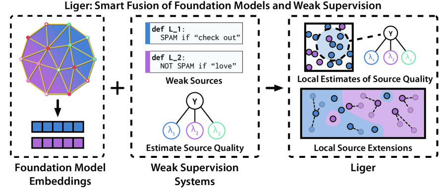
Figure 1: Liger fuses embeddings from foundation models (left) with weak supervision (middle) by exploiting local smoothness of the representations (right). Liger uses the embeddings to a) produce more accurate local estimates of weak source quality (right, top), and b) to locally extend weak sources, improving their coverage (right, bottom).

Foundation models—large pretrained models such as GPT-3, BERT, CLIP, and DALL-E [8, 15, 32, 34]—offer powerful representations that can be used in a broad array of settings [7]. These models have achieved state-of-the-art performance on many tasks. However, it remains unclear how to best apply foundation models in situations where users lack access to any labeled data but do have some weak signals. These are the cases where another class of techniques—weak supervision [35, 16]—shines.

The broad success of foundation models (FMs) suggests that fusing them with weak supervision may offer substantial benefits. Intuitively, the signals present in both can be used to replace large amounts of hand-labeled data in supervised learning. These signals are complementary. Foundation models are trained on huge amounts of data and thus offer powerful general-purpose embeddings. Weak supervision frameworks rely on multiple weak sources of signal that can be synthesized into pseudolabels for downstream training. These weak sources typically express specialized domain expertise. The fusion may enable each component to be improved: FM embeddings can be used without labeled data, while weak sources may be extended to be more general-purpose.

Our goal is to combine these complementary signals to address two challenges in existing approaches to weak supervision. The first challenge is performing fine-grained estimation of source quality. Current weak supervision approaches typically coarsely model source quality by assuming error distributions are uniform over unlabeled points [36, 16], but source quality may vary across points in actuality. The second challenge is producing votes on points where sources abstain. Weak sources often abstain, so that current approaches suffer from low coverage and have many points lacking any signal. We seek to exploit the powerful embeddings from FMs—and the geometry induced by them—to address these challenges.

We propose Liger, a new weak supervision approach based on the notion of local quality of weak sources in the FM embedding space (named after a well-known fusion of powerful animals). We introduce an efficient algorithm that partitions the embedding space and learns per-part local source accuracies. Liger also extends weak sources into nearby regions of the embedding space that they previously abstained on, improving coverage. Despite the fact that FMs are typically black-box, our localized approach exploits a simple measurable notion of their signal: the smoothness of the label distribution in the embedding space. When the distribution of label values does not vary significantly over an embedding region, local source accuracies can be estimated well, and local source extensions maintain their accuracy. We introduce generalization error bounds that individually characterize the impact of partitioning and extending. These error bounds scale in the embedding smoothness and involve a bias-variance tradeoff in the number of partitions and the radii that specify extensions, suggesting that careful incorporation of the FM’s signal into our approach is necessary.

We evaluate Liger on six benchmark NLP and video weak supervision tasks, fusing weak sources with GPT-3 embeddings [8, 30] for the NLP tasks, and with image embeddings from CLIP [32] for the video tasks. We compare Liger against using FMs or weak supervision on their own, as well as baseline techniques for fusing them together. First, Liger outperforms two strong baselines for traditional supervision of FMs, kNN and adapters [21], by 7.2 points, and outperforms traditional weak supervision by 14.1 points. Next, Liger outperforms kNN or adapter-based fusions of weak supervision and FMs by 11.8 points. We find that lift scales with embedding smoothness—confirming our theoretical findings. We measure the smoothness of CLIP embeddings against BiT-M [25], ResNet-101 embeddings pretrained on ImageNet [37], and raw pixels on a video task. We find that CLIP embeddings are smoothest and result in the best performance. Similarly, we find that using the right prompt for GPT-3 has a strong effect on smoothness and performance on a relation extraction task.

In summary, we contribute:

• Liger, a new approach for fusing foundation models with weak supervision by exploiting local smoothness of labels and weak sources in embedding space.

• Finite-sample generalization error bounds of our algorithm that scale in this smoothness.

• Evaluation of Liger on six benchmark NLP and video weak supervision tasks, where Liger outperforms simple fusions of foundation models and weak supervison, as well as either on its own.

2 Background

We describe the problem setting for weak supervision (Section 2.1). We introduce two general challenges in weak supervision that our approach using foundation model embeddings can mitigate. We then propose a model and explain its two stages—source quality estimation and pseudolabel inference (Section 2.2). We provide a brief background on the estimation technique from [16], on top of which we build our approach.

2.1 Problem Setup

Our goal is to predict label $y\in\mathcal{Y}=\{-1,+1\}$ from datapoints $x\in\mathcal{X}$. If we had access to pairs $(x,y)$, we could train a supervised model. However, we do not have access to any samples of $y$; instead, we observe $m$ weak sources $\bm{\lambda}=\{\lambda_{1},\dots,\lambda_{m}\}$, each voting or abstaining on each point $x$ via a probabilistic labeling function $\lambda_{j}:\mathcal{X}\rightarrow\mathcal{Y}\cup\{0\}$ for all $j\in[m]$. We refer to $\lambda_{j}(x)=0$ as an abstain, which occurs when a source is uncertain or not applicable on a point.

We also have access to FM embeddings. These embeddings are the outputs of a mapping $f:\mathcal{X}\rightarrow\mathcal{Z}$ from input space to an embedding space $\mathcal{Z}$ equipped with metric $\rho:\mathcal{Z}\times\mathcal{Z}\rightarrow\mathbb{R}^{+}$. This mapping is fixed and obtained from an off-the-shelf model. Overall, we have an unlabeled dataset $\mathcal{D}=\{x_{i}\}_{i=1}^{n}$ of $n$ i.i.d. points, as well as access to $m$ weak sources and the embedding map $f$.

Given an input $x$ and $\bm{\lambda}(x)$, we aim to learn a label model that predicts $y$ by estimating $\hat{\Pr}(y|\bm{\lambda},x)$ (we drop the $x$ in $\bm{\lambda}(x)$ when obvious). The goal of the label model is to combine sources based on their individual accuracies (i.e. $\lambda_{i}$’s rate of agreement with $y$) by upweighting high-quality sources and downweighting low-quality ones. The resulting pseudolabels given by $\hat{\Pr}(y|\bm{\lambda},x)$ can be used to train a downstream supervised end model or used just directly as predictions. The latter case is often ideal, since users need not train an additional model. We focus on this setting.

Two Challenges and Opportunities. Next, we describe two challenges common to weak supervision techniques. Fusing weak supervision with FM embeddings presents opportunities to mitigate these challenges.

• Coarse Accuracy Modeling. The most common assumption in weak supervision is to model $\hat{\Pr}(y|\bm{\lambda},x)$ as $\hat{\Pr}(y|\bm{\lambda})$. That is, conditioned on the weak sources, the true label is viewed as independent of the features, so only one set of accuracies is learned over the data. Removing this assumption is desirable, since the feature space may have information about the task not captured fully by weak sources. However, naively attempting to model per-point accuracies leads to noisy estimation.

• Low Coverage. Weak sources frequently abstain, leading to low coverage—a situation where much of the dataset has no votes. A simple mitigation is to extend votes from nearby non-abstaining points, but this is risky if the notion of distance is not well-aligned with the label distribution.

An intuitive way to tackle these two challenges is to operate locally. Suppose the source votes and the true label satisfy some level of smoothness such that within some local region of the feature space, they have a low probability of changing values. We can then model accuracies specific to such local regions and can extend source votes to points they abstain on within the regions. However, raw image and text features may lack signal and not offer sufficient smoothness to permit operating locally. By acting on the embedding space, the desired smoothness property is improved (see Figure 2). We can thus obtain finer-grained accuracy estimation and improved coverage by using FM embeddings to model local accuracies and extend locally.

Next, we make these notions concrete by presenting the explicit model for $\Pr(y,\bm{\lambda}|x)$.

2.2 Label Model

We model $\Pr(y,\bm{\lambda}|x)$ as a probabilistic graphical model. Our use of this model has two steps. First, in training, we must estimate the accuracy parameters of $\Pr(y,\bm{\lambda}|x)$ without access to $y$. Then, at inference, we compute $\hat{\Pr}(y|\bm{\lambda},x)$.

Let the graphical model be based on $G=(V,E)$, where $V=y\cup\bm{\lambda}$ and $E$ consists of edges from $y$ to each $\lambda_{j}$ (see Figure 1 middle). For simplicity, we assume there are no dependencies between the weak sources, although the dependencies can be learned [44] and handled by our choice of base estimator from [16]. Therefore, our approach can be extended to that case as well. We model the data distribution as

$$\Pr(y,\bm{\lambda}|x)=\frac{1}{Z}\exp \Big{(}\underbrace{\theta_{y}(x)y}_{\text{Class Balance}}+\sum_{i=1}^{m}\underbrace{\theta_{i}(x)\lambda_{i}y}_{\text{Source Accuracy}}+\sum_{i=1}^{m}\underbrace{\theta_{i,0}(x)\mathbbm{1}\left\{\lambda_{i}=0\right\}}_{\text{Abstain Rate}}\Big{)}$$ (1)

with partition function $Z$ and a set of canonical parameters per $x$, $\Theta(x)=\{\theta_{y}(x),\theta_{i}(x),\theta_{i,0}(x)\;\forall i\in[m]\}$. An important property above is that $\lambda_{i}\mathchoice{\mathrel{\hbox to0.0pt{$\displaystyle\perp$\hss}\mkern 2.0mu{\displaystyle\perp}}}{\mathrel{\hbox to0.0pt{$\textstyle\perp$\hss}\mkern 2.0mu{\textstyle\perp}}}{\mathrel{\hbox to0.0pt{$\scriptstyle\perp$\hss}\mkern 2.0mu{\scriptstyle\perp}}}{\mathrel{\hbox to0.0pt{$\scriptscriptstyle\perp$\hss}\mkern 2.0mu{\scriptscriptstyle\perp}}}\lambda_{j}|y,x\;\forall i,j\in[m]$.

The model concretely portrays the two challenges in weak supervision. First, canonical parameters $\Theta(x)$ that are a function of the input can capture varying accuracy across the data. This is less strict than prior formulations that model the marginal $\Pr(y,\bm{\lambda})$ with one set of canonical parameters without considering input data. However, estimating $\Theta(x)$ is challenging; parametric approaches require certain assumptions on the function $\Theta$ as well as the distribution of $x$ in order to recover the ground truth labels, but these assumptions (e.g., Gaussian $x$) are often not realistic. Standard nonparametric approaches have a high computational complexity and rely on smoothness of the input space $\mathcal{X}$. Second, when $\lambda_{i}(x)=0$, the weak source provides no information on $x$ at inference and is thus typically ignored on that point in previous approaches. This is reflected in the graphical model by Lemma 2 in Appendix C.1, by which $\Pr(y|\lambda_{i}=0,\bm{\lambda}\backslash\lambda_{i},x)=\Pr(y|\bm{\lambda}\backslash\lambda_{i},x)$. In fact, the weak sources provide no direct signal on $x$ when $\bm{\lambda}(x)=\vec{0}$.

Pseudolabel Inference. To perform inference, we compute $\hat{\Pr}(y|\bm{\lambda},x)$ for some $x\in\mathcal{X}$. This is done via Bayes’ rule and the conditional independence of weak sources: $\Pr(y|\bm{\lambda},x)=\prod_{i=1}^{m}\Pr(\lambda_{i}|y,x)\Pr(y|x)/\Pr(\bm{\lambda}|x)$. The latent parameter of interest in this decomposition is $\Pr(\lambda_{i}|y,x)$, which corresponds to the accuracy of $\lambda_{i}$.

Source Parameter Estimation. Previous approaches have considered how to estimate $\Pr(\lambda_{i}|y)$ in a model of $\Pr(\lambda,y)$ via the triplet method [16], using conditional independence properties. For our setting, (1) tells us that $\lambda_{i}y\mathchoice{\mathrel{\hbox to0.0pt{$\displaystyle\perp$\hss}\mkern 2.0mu{\displaystyle\perp}}}{\mathrel{\hbox to0.0pt{$\textstyle\perp$\hss}\mkern 2.0mu{\textstyle\perp}}}{\mathrel{\hbox to0.0pt{$\scriptstyle\perp$\hss}\mkern 2.0mu{\scriptstyle\perp}}}{\mathrel{\hbox to0.0pt{$\scriptscriptstyle\perp$\hss}\mkern 2.0mu{\scriptscriptstyle\perp}}}\lambda_{j}y|\lambda_{i}\wedge\lambda_{j}\neq 0,x$ for any $i\neq j$ (Lemma 3 in Appendix C.1). As a result, $\mathbb{E}\left[\lambda_{i}y|\lambda_{i}\neq 0,x\right]\times\mathbb{E}\left[\lambda_{j}y|\lambda_{j}\neq 0,x\right]=\mathbb{E}\left[\lambda_{i}\lambda_{j}y^{2}|\lambda_{i}\wedge\lambda_{j}\neq 0,x\right]=\mathbb{E}\left[\lambda_{i}\lambda_{j}|\lambda_{i}\wedge\lambda_{j}\neq 0,x\right]$, which consists of observable variables. Define $a_{i}(x)=\mathbb{E}\left[\lambda_{i}y|\lambda_{i}\neq 0,x\right]$ as the accuracy of $\lambda_{i}$ on $x$. If we introduce a third $\lambda_{k}$, we can generate a system of equations over $a_{i}(x),a_{j}(x),a_{k}(x)$ in terms of the conditional expected products of pairs of $\lambda_{i},\lambda_{j},\lambda_{k}$. As a result,

$$|a_{i}(x)|:=\sqrt{\bigg{|}\frac{\mathbb{E}\left[\lambda_{i}\lambda_{j}|\lambda_{i}\wedge\lambda_{j}\neq 0,x\right]\mathbb{E}\left[\lambda_{i}\lambda_{k}|\lambda_{i}\wedge\lambda_{k}\neq 0,x\right]}{\mathbb{E}\left[\lambda_{j}\lambda_{k}|\lambda_{j}\wedge\lambda_{k}\neq 0,x\right]}\bigg{|}},$$ (2)

and likewise for $\hat{a}_{j}(x),\hat{a}_{k}(x)$. More details are in Appendix C.2. (1) allows us to write $\Pr(\lambda_{i}|y,x)=\frac{1+\textrm{sgn}(\lambda_{i}y)a_{i}(x)}{2}\times\Pr(\lambda_{i}\neq 0|x)$ (Lemmas 2 and 4), so the desired probability estimate is just a linear transformation of $a_{i}(x)$ scaled by $\lambda_{i}$’s coverage.

3 Fusion Algorithm

We are ready to present Liger, our approach to fusing foundation model embeddings and weak supervision. We explain the two components: first, how to compute conditional estimates of the label model parameters over local regions of the partitioned embedding space for finer-grained accuracy estimation; second, how to extend weak sources via a kNN-like augmentation in the embedding space, improving their coverage and hence the signal available at inference. The full approach is shown in Algorithm 1.

  Input: Dataset $\mathcal{D}=\{x_{i}\}_{i=1}^{n}$, weak sources $\bm{\lambda}$, embedding mapping $f$ and metric $\rho$, threshold radii $r_{1},\dots r_{m}$, partition $\mathcal{C}$ and class balances $\Pr(y|C_{j})$ for $j\in[s]$.

  Returns: Label model $\hat{\Pr}(y|\bm{\bar{\lambda}},x)$.

  for $\lambda_{i}\in\bm{\lambda}$ do

      Construct extended source $\bar{\lambda}_{i}$ using $r_{i},f,\rho$ as in (3).

  end for

  for $C_{j}\in\mathcal{C}$ do

      for $\bar{\lambda}_{i}\in\bm{\bar{\lambda}}$ do

         Compute accuracy $\hat{a}_{i}(C_{j})$ using Algorithm 2 on $\bar{\lambda}_{i}$ over $C_{j}$, and compute coverage $\hat{\Pr}(\bar{\lambda}_{i}\neq 0|C_{j})$ on $\mathcal{D}$.

         Set $\hat{\Pr}(\bar{\lambda}_{i}|y,C_{j})$ equal to $\frac{1+\textrm{sgn}(\bar{\lambda}_{i}y)\hat{a}_{i}(C_{j})}{2}\hat{\Pr}(\bar{\lambda}_{i}\neq 0|C_{j})$ for $\bar{\lambda}_{i}\in\{-1,1\}$, $\hat{\Pr}(\bar{\lambda}_{i}=0|C_{j})$ otherwise.

      end for

      Compute $\hat{\Pr}(\bm{\bar{\lambda}}|C_{j})$ on $\mathcal{D}$.

  end for

  return  For test point $x\in\mathcal{X}$, compute $\hat{\Pr}(y|\bm{\bar{\lambda}},x)=\hat{\Pr}(y|\bm{\bar{\lambda}},C(x))=\frac{\prod_{i=1}^{m}\hat{\Pr}(\bar{\lambda}_{i}|y,C(x))\Pr(y|C(x))}{\hat{\Pr}(\bm{\bar{\lambda}}|C(x))}$.

Algorithm 1 Liger

Local Parameter Estimation

Our first task is to compute the label model’s local parameters. Based on (2), the quantities to estimate are of the form $\mathbb{E}\left[\lambda_{i}\lambda_{j}|\lambda_{i}\wedge\lambda_{j}\neq 0,x\right]$, $\Pr(\lambda_{i}\neq 0|x)$, $\Pr(\bm{\lambda}|x)$, $\Pr(y|x)$. These conditional statistics can be estimated using nonparametric approaches such as the Nadaraya-Watson estimator, but they require $\mathcal{O}(n)$ computations per point at inference.

Instead of estimating parameters per point, we partition the embedding space and compute per-part statistics. Intuitively, this choice exploits smoothness. If label distributions are smooth, i.e., they do not vary greatly within a local region, it is sufficient to estimate per-point statistics using a part given that parts are not too large. Controlling the size of the partition is thus important in determining how well we can approximate per-point statistics.

Concretely, partition $\mathcal{Z}$ into $s$ subsets $\mathcal{C}=\{C_{1},\dots,C_{s}\}$ of equal size $n^{\prime}=\frac{n}{s}$ (we use K-means clustering with $K=s$ in practice). Denote $C(x)$ as the subset $f(x)$ belongs to. Instead of estimating statistics and performing inference conditioned on $x$, we condition on $C(x)$, producing $s$ sets of parameters overall. We estimate $\mathbb{E}\left[\lambda_{i}\lambda_{j}|\lambda_{i}\wedge\lambda_{j}\neq 0,C(x)\right]$, yielding a local accuracy estimate $\hat{a}_{i}(C(x))$ formalized in Algorithm 2, as well as $\Pr(\lambda_{i}\neq 0|C(x))$, $\Pr(\bm{\lambda}|C(x))$, $\Pr(y|C(x))$. Then, we use $\hat{\Pr}(y|\bm{\lambda},x)=\hat{\Pr}(y|\bm{\lambda},C(x))$ as our label model prediction on $x$. These estimates are done over the subsets; for instance, $\Pr(\bm{\lambda}|C(x))\approx\frac{1}{n^{\prime}}\sum_{x^{\prime}\in C(x)}\mathbbm{1}\left\{\bm{\lambda}(x^{\prime})\texttt{=}\bm{\lambda}\right\}$. We assume that class balance on subsets, $\Pr(y|C(x))$, are known. There are also several techniques that can be used to estimate these [36], or they can be treated as hyperparameters.

Weak Source Extension

Next, we improve the model of $\hat{\Pr}(y|\bm{\lambda},x)$ by increasing source coverage. Let $\bar{\lambda}_{i}$ be an extended labeling function with corresponding threshold radius $r_{i}>0$ for $i\in[m]$. The extension works as follows. For any $x$, let $\text{NN}(x)=\textrm{argmin}_{x^{\prime}\in\mathcal{D}:\lambda_{i}(x)\neq 0}~{}\rho(f(x),f(x^{\prime}))$ be the nearest neighbor of $x$ in embedding space from $\mathcal{D}$ such that $\lambda_{i}$ has coverage on it. $\bar{\lambda}_{i}$ uses nearest neighbors to weakly label points within $r_{i}$ of $\lambda_{i}$’s support on $\mathcal{D}$. Formally,

$$\bar{\lambda}_{i}(x):=\begin{cases}\lambda_{i}(x)&\lambda_{i}(x)\neq 0\\ \lambda_{i}(\text{NN}(x))&\rho(f(x),f(\text{NN}(x)))\leq r_{i}\\ 0&\text{o.w.}\end{cases}.$$ (3)

We can view $\bar{\lambda}_{i}$ as an augmentation on $\lambda_{i}$ using $\mathcal{D}$ and $f$. We thus perform parameter estimation and inference using $\bm{\bar{\lambda}}$ instead of $\bm{\lambda}$, namely learning $\Pr(y|\bm{\bar{\lambda}},C(x))$.

There are two advantages to using extended sources. First, extended sources improve sampling error, since expressions like $\mathbb{E}\left[\lambda_{i}\lambda_{j}|\lambda_{i}\wedge\lambda_{j}\neq 0,x\right]$ are estimated over more data in $\mathcal{D}$. Second, $\bar{\lambda}_{i}$ provides signal at inference on points that $\lambda_{i}$ previously abstains on. However, the quality of this signal greatly depends on $r_{i}$. If $\lambda_{i}$ is overextended and the embedding space is not sufficiently smooth, points far away from $\lambda_{i}$’s support may receive incorrect extended source votes, suggesting that careful choice of $r_{i}$ is needed.

Our approach combines the two components discussed—partitioning the embedding space and extending sources—to output predictions $\hat{\Pr}(y|\bm{\bar{\lambda}},C(x))$ as in Algorithm 1. Note that our approach builds on the algorithm from [16], but partitioning and extending can also be done on top of other weak supervision algorithms that model things differently.

4 Theoretical Analysis

Now we turn to analyzing Algorithm 1. Our goal is to understand how performance depends on the key parameters: fineness of the partition $\mathcal{C}$, radii $r_{i}$ of the extensions used to improve coverage, and smoothness of the embedding space.

We begin with a result on the generalization error of the label model $\hat{\Pr}(y|\bm{\lambda},x)$, which relies on the number of partitions $s$ to control the granularity of the estimated parameters (Theorem 1). Then, we discuss the improvement from using $\bm{\bar{\lambda}}$ instead of $\bm{\lambda}$. We first bound the local accuracy of an extended source in a region it previously abstains (Lemma 1), and then we show that as long as this local accuracy is better than random, we can further reduce the generalization error (Theorem 2). The former result presents a bias-variance tradeoff depending on $s$, while the latter has a tradeoff dependent on the threshold radius $r_{i}$. In both cases, $s$ and $r_{i}$ must be carefully set based on the signal in the FM embeddings, namely the smoothness of label distributions in the FM embedding space, in order to optimize performance. We provide proofs in Appendix D, synthetic experiments supporting our findings in Appendix F.3, and smoothness measurements on real data in Section 5.2 and Appendix F.2.

Define the generalization error of the label model using weak sources $\bm{\lambda}$ as the expected cross-entropy loss, $L(\bm{\lambda})=\mathbb{E}_{\mathcal{D},x,y,\bm{\lambda}}[-\log\hat{\Pr}(y|\bm{\lambda},x)]$.

4.1 Label Model Generalization Error

We bound the generalization error $L(\bm{\lambda})$ of the label model using the unextended, initial weak sources. The key quantity in this analysis is embedding smoothness:

Definition 1 (Lipschitzness).

The distributions $\Pr(y|x)$ and $\Pr(\lambda_{i}|y,x)$ are Lipschitz-smooth on the metric space $(\mathcal{Z},\rho)$ with constants $K_{y},K_{\lambda},K_{\lambda,0}>0$ if for all $i\in[m]$,

$$|\Pr(y=1|x)-\Pr(y=1|x^{\prime})|\leq K_{y}\rho(f(x),f(x^{\prime})),$$

$$|\Pr(\lambda_{i}=1|y,\lambda_{i}\neq 0,x)-\Pr(\lambda_{i}=1|y,\lambda_{i}\neq 0,x^{\prime})|\leq K_{\lambda}\rho(f(x),f(x^{\prime})),$$

$$|\Pr(\lambda_{i}\neq 0|x)-\Pr(\lambda_{i}\neq 0|x^{\prime})|\leq K_{\lambda,0}\rho(f(x),f(x^{\prime})),$$

We refer to these three properties as label, source, and coverage Lipschitzness, respectively.

In words, if the constants $K_{y},K_{\lambda},K_{\lambda,0}$ are small, the class balance of $y$ and the way each source votes (or doesn’t) do not vary significantly over a local region of the embedding space.

We define some additional quantities. Set $\alpha=\max_{i}\mathbb{E}_{x}\left[\frac{1}{p_{ij}}\;\big{|}\;p_{ij}\neq 0\right]$, where $p_{ij}=\Pr(\lambda_{i}\neq 0|f(x)\in C_{j})$ is the coverage of $\lambda_{i}$ on $C_{j}$, to be the largest average inverse source coverage over the subsets. $\alpha$ corresponds to how often sources abstain. Assume that $a_{i}(C_{j})>0$ for all $\lambda_{i}$ and $C_{j}$, meaning that the average source accuracy on a subset is better than random. Then, define $a_{\max}=\max_{i,j}a_{i}(C_{j})$, and $b_{\min}=\min\limits_{i,j,k}\{\mathbb{E}\left[\lambda_{i}\lambda_{k}|\lambda_{i}\wedge\lambda_{k}\neq 0,C_{j}\right],\hat{\mathbb{E}}\left[\lambda_{i}\lambda_{k}|\lambda_{i}\wedge\lambda_{k}\neq 0,C_{j}\right]\}$ as the minimum rate of agreement between sources over subsets, where $\hat{\mathbb{E}}$ denotes the empirical estimate on $\mathcal{D}$. Define $d_{C_{j}}=\max_{f(x),f(x^{\prime})\in C_{j}}\rho(f(x),f(x^{\prime}))$ as the diameter of $C_{j}$ and $d_{\mathcal{C}}=\mathbb{E}_{x}\left[d_{C(x)}\right]$ as its average.

Theorem 1.

Suppose that data $x,y,\bm{\lambda}$ follows the model in (1) and $\Pr(y|x)$ and $\Pr(\lambda_{i}|y,x)$ for each $\lambda_{i}$ are Lipschitz-smooth. The generalization error of the label model $\hat{\Pr}(y|\bm{\lambda},x)$ in Algorithm 1 when $r_{i}=0\;\forall i$ can be decomposed into $L(\bm{\lambda})\texttt{=}\text{Bias}+\text{Variance}+\text{Irreducible Error}+o(1/n)$, where

$$\text{Bias}\leq 2d_{\mathcal{C}}(K_{y}+mK_{\lambda}+mK_{\lambda,0}),$$

$$\text{Variance}\leq\frac{ms}{n}\bigg{(}\frac{3\alpha(1-b_{\min}^{2})}{8b_{\min}^{2}(1-a_{\max}^{2})}\Big{(}\frac{1}{b_{\min}^{4}}+\frac{2}{b_{\min}^{2}}\Big{)}+1\bigg{)},$$

$$\text{Irreducible Error}=H(y|\bm{\lambda},x),$$

where $H(y|\bm{\lambda},x)$ denotes conditional entropy.

We discuss each term of this bound.

• The bias comes from the partition $\mathcal{C}$, since conditional statistics on $C(x)$ are not equivalent to those on $x$. When the embedding space is smooth with small $K_{y},K_{\lambda},K_{\lambda,0}$, the bias is low. Note that making the subset diameter $d_{C}\rightarrow 0$ makes the bias go to zero.

• The variance comes from sampling error in Algorithm 2 and $\hat{\Pr}(\lambda_{i}\neq 0|C_{j})$. This quantity scales in $\mathcal{O}(s\alpha/n)$ and also depends on accuracy and agreement among weak sources.

• The irreducible error depends on quality of $\bm{\lambda}$. If knowledge of $\bm{\lambda}$ significantly reduces uncertainty in $y$, i.e., the sources contain lots of signal, this quantity is low. On the other hand, $H(y|\bm{\lambda},x)$ is maximized when $\bm{\lambda}\mathchoice{\mathrel{\hbox to0.0pt{$\displaystyle\perp$\hss}\mkern 2.0mu{\displaystyle\perp}}}{\mathrel{\hbox to0.0pt{$\textstyle\perp$\hss}\mkern 2.0mu{\textstyle\perp}}}{\mathrel{\hbox to0.0pt{$\scriptstyle\perp$\hss}\mkern 2.0mu{\scriptstyle\perp}}}{\mathrel{\hbox to0.0pt{$\scriptscriptstyle\perp$\hss}\mkern 2.0mu{\scriptscriptstyle\perp}}}y|x$, i.e. there is no signal about $y$ in $\bm{\lambda}$.

Our result reveals a bias-variance tradeoff dependent on the number of parts $s$. As $s$ increases, subset diameter $d_{\mathcal{C}}$ tends to decrease, resulting in lower bias because the subset parameters estimated will be closer in true value to those conditional on $x$. The variance increases in $s$ because there are fewer points per subset for estimation. The $s=1$ case, which incurs a large bias, is algorithmically equivalent to the approach in [16]. Such approaches thus suffer from model misspecification in our setting—and likely in most practical cases—as they assume uniform quality per source.

4.2 Improvement from Extensions

Suppose that $x,y,\bm{\bar{\lambda}}$ follows (1). When we use $\bm{\bar{\lambda}}$ rather than $\bm{\lambda}$ (i.e. $r_{i}\neq 0$), there are several changes to the decomposition in Theorem 1:

• The bias is now bounded by $2d_{\mathcal{C}}K_{y}+2m(d_{\mathcal{C}}+2\max_{i}r_{i})(K_{\lambda}+K_{\lambda,0})$ (see Lemma 8 in Appendix D). We must consider when $\text{NN}(x)$ is not in $C(x)$, essentially resulting in a wider subset diameter.

• The variance is still $\mathcal{O}(1/n)$, but multiplicative factors change. For instance, $\alpha$ decreases due to improved coverage, thus decreasing the variance.

• The irreducible error is now $H(y|\bm{\bar{\lambda}},x)$.

We analyze $H(y|\bm{\bar{\lambda}},x)$ in this section. $\bar{\lambda}_{i}$ provides more signal than $\lambda_{i}$ at inference on points where $\lambda_{i}(x)=0$, but the signal about $y$’s value may be incorrect. Extending $\lambda_{i}$ using too large of $r_{i}$ could yield incorrect source votes, resulting in lower accuracy of the extended weak source.

We first present a result on how $r_{i}$ controls the extended source’s accuracy. Define $a_{i}=\mathbb{E}\left[\lambda_{i}y|\lambda_{i}\neq 0\right]$ as the average accuracy of $\lambda_{i}$, and $\bar{a}_{i}(r_{i})=\mathbb{E}\left[\bar{\lambda}_{i}y|\bar{\lambda}_{i}\neq 0,\lambda_{i}=0\right]$ as $\bar{\lambda}_{i}$’s average accuracy on the extended region. We also need a notion of smoothness of $y$ between the original support and the extended region. We define a local notion of probabilistic Lipschitzness (PL), originally introduced in [43].

Definition 2 (Probabilistic Lipschitzness).

Define $\mathcal{P}_{\lambda_{i}}=\Pr_{x,y}(\cdot|\lambda_{i}\neq 0)$ to be the distribution of $(x,y)$ over the support of $\lambda_{i}$, and let $\mathcal{P}_{\lambda_{i},x}$ be its marginal distribution on $x$. Then $\mathcal{P}_{\lambda_{i}}$ is $M$-probabilistically Lipschitz for an increasing function $M:\mathbb{R}^{+}\rightarrow[0,1]$ if for any $r>0$,

$$\Pr_{x,y\sim\mathcal{P}_{\lambda_{i}}}(\exists(x^{\prime},y^{\prime}) \in\mathcal{X}\backslash\text{supp}(\mathcal{P}_{\lambda_{i},x})\times\mathcal{Y}:\rho(f(x),f(x^{\prime}))\leq r,y^{\prime}\neq y)\leq M(r).$$

We refer to this property as local label PL.

In words, the probability that there is a point outside of the support of $\lambda_{i}$ but within $r$ of $(x,y)\sim\mathcal{P}_{\lambda_{i}}$ with a different label from $y$ is bounded by an increasing function of $r$. We also define $\beta_{i}=\mathbb{E}[\lambda_{i}y|\lambda_{i}\neq 0,\exists(x^{\prime},y^{\prime}):\lambda_{i}(x^{\prime})=0,\rho(f(x),f(x^{\prime}))\leq r_{i},y^{\prime}=y]$ as $\lambda_{i}$’s accuracy over a region close to where $\lambda_{i}$ is extended and $y$ changes value.

With this definition, we show that:

Lemma 1.

Suppose $\mathcal{P}_{\lambda_{i}}$ is $M$-probabilistically Lipschitz. The average accuracy of $\bar{\lambda}_{i}$ on the extended region is at least $\bar{a}_{i}(r_{i})\geq a_{i}-(1+\beta_{i})M(r_{i})$.

Our result provides local accuracy guarantees on $\bar{\lambda}_{i}$ as a function of the original $\lambda_{i}$’s accuracy, the probabilistic Lipschitzness of the embedding space, and the $r_{i}$ the user sets. Extending a source with higher original accuracy will yield stronger accuracy guarantees in the extended region. On the other hand, if $M(r_{i})$ is too large due to improper $r_{i}$ or lack of smoothness, the true label is more likely to change value, and hence accuracy in the extended region worsens.

Now we can use our result on $\bar{a}_{i}(r_{i})$ to analyze the improvement in irreducible error. We extend just one weak source $\lambda_{i}$ by $r_{i}$ and keep $\lambda_{-i}:=\bm{\lambda}\backslash\lambda_{i}$ unextended. Define $p_{i}=\Pr(\bar{\lambda}_{i}\neq 0,\lambda_{i}=0)$ as the proportion of the region where $\bar{\lambda}_{i}$ is extended and $p(\lambda_{-i})=\mathbb{E}_{y^{\prime},\lambda_{-i},\bar{\lambda}_{i}\neq 0,\lambda_{i}=0}\left[\Pr(y=y^{\prime}|\lambda_{-i},x)\right]$ as the label model’s probability of outputting the correct label in the extension region when only using $\lambda_{-i}$.

Theorem 2.

Suppose that data follows the model in (1). The irreducible error decreases by at least the following amount when using $\bar{\lambda}_{i}$ rather than $\lambda_{i}$ in Algorithm 1:

$$H(y|\bm{\lambda},x)-H(y|\bm{\bar{\lambda}},x)\geq 2p_{i}(1-p(\lambda_{-i}))^{2}\cdot\bar{a}_{i}(r_{i})^{2}.$$

Lift increases with probability mass $p_{i}$ on the extended region since more of the data is impacted by $\bar{\lambda}_{i}$. Lift is not as significant if $p(\lambda_{-i})$ is large because the other weak sources already are providing sufficient signal for $y$. Most importantly, lift scales with how far $\bar{a}_{i}(r_{i})$ is from $0$ (random voting). This highlights a tradeoff in $r_{i}$: as $r_{i}$ increases, $p_{i}$ increases but the lower bound on $\bar{a}_{i}(r_{i})$ from Lemma 1 decreases. This shows that threshold radii must be selected carefully; if the embedding space has strong probabilistic Lipschitzness (i.e. small $M$) or the original weak source has high accuracy, then the source can be extended further while providing lift. However, overextension of the source can yield low local accuracy and thus less lift.

Our results demonstrate that $s$ and $r_{i}$ control the label model’s performance, and setting these terms depends on how smooth label distributions are in the embedding space.

5 Experiments

		Weak Sources Only
	Task	WS-kNN	WS-Adapter	WS-LM	Liger	$\Delta$Coverage
NLP	Spam	72.8	92.3	83.6	95.0	+45.5
	Weather	62.0	86.0	78.0	98.0	+90.2
	Spouse	16.9	17.1	47.0	52.2	+12.1
Video	Basketball	33.3	48.9	27.9	69.6	+8.3
	Commercial	84.7	92.8	88.4	93.5	+18.8
	Tennis	83.0	83.8	82.0	83.3	+32.5

Dev Labels Available
kNN	Adapter	Liger-Adapter
91.2	94.4	95.4
92.0	90.0	96.8
21.6	15.7	49.6
64.4	79.3	79.5
92.0	93.0	93.2
73.2	83.1	84.0

Table 1: Left: Liger performance compared to baselines that only have access to weak labels, as well as the change in coverage from traditional weak supervision. Right: Liger-Adapter performance compared to baselines that have access to dev labels. Scores are F1 except for Spam and Weather (accuracy); best score in bold in each setting.

This section evaluates the following claims about Liger:

• Performance (Section 5.1): Liger outperforms vanilla weak supervision, as well as baseline approaches for using foundation models directly, either with traditional weak supervision or hand supervision.

• Smoothness (Section 5.2): Lift is correlated with the smoothness of the label distribution in the representation space. We measure smoothness and performance of CLIP against three other embedding methods on a video task, and measure three prompting strategies for GPT-3 on a relation extraction task.

• Ablations (Section 5.3): Both components of Liger—partitioning the representation space and extending labeling function votes—are important for performance.

Datasets

We evaluate Liger on six benchmark NLP and video tasks used to evaluate previous weak supervision methods [16, 47]. In NLP, Spam identifies spam YouTube comments [3]; Weather identifies the sentiment of weather-related tweets [1]; and Spouse identifies spouse relationships in newspaper articles [13]. In video, Commercial identifies commercial segments in TV news [20, 17]; Tennis identifies rallies in tennis segments; and Basketball identifies basketball videos in a subset of ActivityNet [9]. Each dataset consists of a large unlabeled training set, a smaller hand-labeled development set (train/dev split sizes from 187/50 points to 64,130/9,479 points), and a held-out test set. We use the unlabeled training set to train label models and use the development set for a) training of traditional supervision baselines, and b) hyperparameter tuning of the label models, including $s$ and $r_{i}$.

Pre-trained embeddings

For the NLP datasets, we use pre-trained GPT-3 [8] embeddings from OpenAI’s Ada model. For Spam and Weather, we simply embed the text directly. For Spouse, we add a prompt “Are [person 1] and [person 2] spouses?” after the end of the sentence. We discuss further prompting strategies in Section 5.2. For video datasets, we use image embeddings from CLIP [32] over individual frames of the videos.

Embedding	F1-score
Raw pixel	19.3
RN-101	31.1
BiT-M	42.5
CLIP	69.6

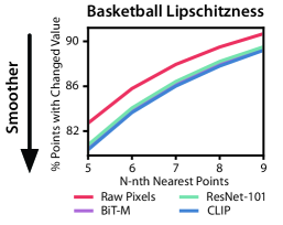
Prompting	F1-score
No Prompt	48.5
Prompt Beginning	50.2
Prompt End	52.2

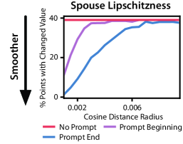
Figure 2: Left: Liger performance and smoothness measurements of CLIP, BiT-M, ResNet-101, and raw pixels as embeddings for Basketball. Right: Liger performance and smoothness measurements of no prompting, prompting at beginning, and prompting at end in GPT-3 for Spouse.

5.1 Performance

We compare Liger against baseline approaches for fusing foundation models with weak supervision, as well as against using either on their own. We split our evaluation into two parts: methods that only have access to weak sources, and methods that additionally have access to the dev set.

Weak Sources Only

We compare the performance of Liger against vanilla weak supervision’s label model (WS-LM) [16], as well as two end models, weakly-supervised kNN (WS-kNN), and weakly-supervised adapters (WS-Adapter). In the latter two methods, we use the predictions from WS-LM to generate pseudolabels for the train set and use the FM embeddings as input data (since we do not access the full FM) to the kNN and adapter approaches. We consider an adapter that is a linear layer on the FM embeddings. We also provide results on 3-layer MLP adapters in Appendix F.

Table 1 (left) shows the results, as well as statistics on the additive change in coverage ($\%$ of the dataset that sources vote on) between Liger and WS-LM. Liger outperforms WS-LM and has better coverage (33.2 points on average). Liger also outperforms both of the baseline approaches for fusing foundation models with weak supervision, WS-kNN and WS-Adapter.

Weak Sources and Dev Labels

Next, we compare performance against methods that have access to a small hand-labeled dev set. We compare against two baselines: kNN and Adapter, both trained over the dev set labels. For our method Liger-Adapter, we train an adapter over Liger labels on the train set, as well as the dev labels. In some cases, Liger labels are too noisy to provide good signal on the train set; in this case, our solution automatically downsamples the pseudolabels on the train set. We also provide the original Liger prediction as input to the adapter. See Appendix E for the details.

Table 1 (right) shows the results. Liger-Adapter outperforms Adapter and kNN. On the datasets where Liger labels are very accurate, we see additional lift from the adapters because we have more points to train on. When the labels are not very accurate, our downsampling prevents the noisy labels from harming adapter performance. In one case, learning an adapter over the embeddings is very hard (Spouse). Here, providing the Liger prediction as input is critical for performance.

5.2 Embedding Smoothness

We measure how smoothness of the embedding space affects the performance of Liger. First, we compare embeddings from CLIP against BiT-M embeddings [25], a ResNet-101 pretrained on ImageNet [37], and raw pixels. Second, we vary the GPT-3 prompting strategy for Spouse and compare against two alternative methods that result in a less smooth representation. We report label Lipschitzness—the smoothness of embeddings with respect to ground-truth labels—in this section. See Appendix F.2 for additional measures of Lipschitzness.

Figure 2 (left) shows the performance of CLIP, BiT-M, ResNet-101, and raw pixels as embeddings for Liger, as well as measures of Lipschitzness for each method (lower is smoother). CLIP embeddings are smoother than the other methods—which matches their performance when used in Liger.

Comparing Prompting Strategies

Next, we examine the impact of prompting strategies for Spouse. Spouse is a relation extraction dataset, where the task is to predict whether two entities in a sentence are married. Since there may be multiple entities in a sentence, Spouse contains multiple duplicate sentences in the dataset, with different labels. To alleviate this problem, we introduce a prompt “Are [person 1] and [person 2] spouses?” after the end of the sentence, where “[person 1/2]” are replaced by the names of the first/second entity in the sentence. We compare this prompting strategy against two others: appending the same prompt to the beginning of the sentence, and leaving the original sentence as-is, without any prompting.

Figure 2 (right) shows the performance and smoothness of each of these prompting methods. Adding the prompt to the end of the sentence results in the best performance and smoothest embeddings. Both methods perform better than leaving the sentence alone (the flat line is a result of multiple sentences with different labels having the same embedding).

5.3 Ablations

Task	Liger ($s$)	-Part	-Ext ($s$)	-Part, -Ext
Spam	95.0 (2)	94.0	92.0 (7)	83.6
Weather	98.0 (3)	96.0	94.0 (5)	78.0
Spouse	52.2 (6)	50.0	49.3 (5)	47.0
Basketball	69.6 (2)	69.6	21.9 (2)	27.9
Commercial	93.5 (3)	92.3	91.4 (5)	88.4
Tennis	83.3 (1)	83.3	81.3 (2)	82.0

Table 2: Ablations of Liger, removing partitions (-Part), extensions (-Ext), and both. Best $s$ values inside parentheses.

We report ablations on each component of Liger. Table 2 removes the partioning component and the extensions component. Partitioning improves performance on four tasks, and extensions improves performance on all tasks (13.1 points of lift on average from partitioning, 3.8 points from extensions). Combining both additionally offers the best performance on four tasks.

6 Related Work

We present an abbreviated related work here. See Appendix A for an extended treatment.

Weak supervision frameworks typically model source accuracies to generate weak labels and then fine-tune an end model for generalization [35, 4, 24, 40, 16, 46, 38, 6]. One framework models the end-to-end process all at once [10], but requires training the end model at the same time—which is computationally expensive with large foundation models. Our work removes the fine-tuning step completely.

Our work is similar to transfer learning techniques, which adapt pretrained models for downstream tasks [25, 14]. Foundation models offer new requirements for transfer learning setting: when it is impossible to fine-tune the original models [7]. We build on approaches such as prompting [27, 8], embedding search [30], and adapters [21, 2].

7 Conclusion

We present Liger, a system for fusing foundation models and weak supervision. We use embeddings to produce finer-grained estimates of weak source accuracies and improve weak source coverage. We prove a series of results on how the performance of this approach scales with the smoothness of the embeddings, and demonstrate Liger on six benchmark NLP and video weak supervision datasets. We hope our work will encourage further work in combining foundation models and weak supervision and in utilizing the signal from foundation models to help with other tasks.

Authors’ Note

The first two authors contributed equally. Co-first authors can prioritize their names when adding this paper’s reference to their resumes.

Appendix

We present an extended related work (Appendix A), glossary (Appendix B), additional algorithmic details (Appendix C), proofs (Appendix D), experimental details (Appendix E), and additional experimental results (Appendix F).

Appendix A Extended Related Work

Weak supervision is a broad set of techniques using weak sources of signal to supervise models, such as distant supervision [42], co-training methods [5], pattern-based supervision [18] and feature annotation [29, 28]. Weak supervision frameworks often train in two stages—first modeling source accuracies to generate weak labels, and then fine-tuning a powerful end model for generalization [35, 4, 24, 40, 16, 46, 38, 6]. Our work removes the second stage from the equation and addresses two common challenges in weak supervision, coarse accuracy modeling and low coverage.

One weak supervision work that does not train in two stages, and models source qualities in a way that can be nonuniform over the points is WeaSuL [10]. However, this capability is present in a different context: end-to-end training of a weak supervision label model with an end model. This prevents the use of the label model directly for prediction, as we seek to do in our work. It requires much heavier computational budget, for example, when training a deep model, which is not needed with our approach. In addition, WeaSuL relies on the use of an encoder for source qualities, rendering a theoretical analysis intractable. By contrast, our approach offers clean and easy-to-interpret theoretical guarantees.

Another recent work that utilizes pre-trained embeddings in weak supervision is from [26]. Their work uses the smoothness of the embedding space to remove low-quality weakly-labeled data points, while we use it to improve coverage and fine-grained estimation to weakly label additional points more accurately.

Transfer learning uses large datasets to learn useful feature representations that can be fine-tuned for downstream tasks [25, 14]. Transfer learning techniques for text applications typically pre-train on large corpora of unlabeled data [14, 8, 33], while common applications of transfer learning to computer vision pre-train on both large supervised datasets such as ImageNet [37] and large unsupervised or weakly-supervised datasets [19, 12, 32]. Pre-trained embeddings have also been used as data point descriptors for kNN search algorithms to improve model performance, interpretability, and robustness [31, 23]. We view our work as complementary to these approaches, presenting another mechanism for using pre-trained networks.

Foundation models offer a new interface for the transfer learning setting: when it is impossible to fine-tune the original models [7]. In this setting, the foundation models can still be used either by direct prompting [27, 8], or by using embeddings [30]. [45] prompts FMs to produce pseudolabels, providing a complementary way to use FMs in weak supervision. In contrast, our work focuses on using FM embeddings. Since we can only access the final embeddings of some foundation models, we focus on adapters [21] over the final layer in this work—which are equivalent to linear probes [2].

Semi-supervised and few-shot learning approaches aim to learn good models for downstream tasks given a few labeled examples. Semi-supervised approaches like label propagation [22] start from a few labeled examples and iteratively fine-tune representations on progressively larger datasets, while few-shot learning approaches such as meta-learning and metric learning aim to build networks that can be directly trained with a few labels [41]. Our work is inspired by these approaches for expanding signal from a subset of the data to the entire dataset using FM representations, but we do not assume that our labeling sources are perfect, and we do not tune the representation.

Appendix B Glossary

The glossary is given in Table 3 below.

Symbol	Used for
$x$	Input data point $x\in\mathcal{X}$.
$y$	True task label $y\in\mathcal{Y}=\{-1,+1\}$.
$\bm{\lambda}$	Weak sources $\bm{\lambda}=\{\lambda_{1},\dots,\lambda_{m}\}$, where each $\lambda_{j}:\mathcal{X}\rightarrow\mathcal{Y}\cup\{0\}$ is a probabilistic labeling function
	that votes on each $x$.
$m$	Number of weak sources.
$f$	A fixed mapping from input space $\mathcal{X}$ to embedding space $\mathcal{Z}$ that is made available by the off-the-shelf
	foundation model.
$\rho$	A fixed metric on the embedding space, $\rho:\mathcal{Z}\times\mathcal{Z}\rightarrow\mathbb{R}^{+}$.
$\mathcal{D}$	A training dataset of $n$ i.i.d. unlabeled points, $\mathcal{D}=\{x_{i}\}_{i=1}^{n}$.
$n$	Number of points in the unlabeled training dataset $\mathcal{D}$.
$G$	The dependency graph $G=(V,E)$ used to model $\Pr(y,\bm{\lambda}|x)$, where $V=y\cup\bm{\lambda}$ and $E$ contains
	edges between $y$ and $\bm{\lambda}$.
$\Theta(x)$	The set of canonical parameters $\Theta(x)=\{\theta_{y}(x),\theta_{i}(x),\theta_{i,0}(x)\;\forall i\in[m]\}$ corresponding to
	class balance, source accuracy, and the abstain rate used to parametrize $\Pr(y,\bm{\lambda}|x)$ in (1).
$Z$	Partition function used for normalizing the distribution of $\Pr(y,\bm{\lambda}|x)$.
$a_{i}(x)$	Accuracy parameter of $\lambda_{i}$ on point $x$, $a_{i}(x)=\mathbb{E}\left[\lambda_{i}y|\lambda_{i}\neq 0,x\right]$.
$\mathcal{C}$	Partition of the embedding space $\mathcal{Z}$ into nonoverlapping subsets, $\mathcal{C}=\{C_{1},\dots,C_{s}\}$.
$s$	Size of the partition $\mathcal{C}$.
$n^{\prime}$	The number of points from $\mathcal{D}$ in each subset $C_{j}$, $n^{\prime}=\frac{n}{s}$.
$C(x)$	The subset that $x$ belongs to, i.e. $C(x)=C_{j}$ if $f(x)\in C_{j}$.
$a_{i}(C(x))$	Local accuracy parameter of $\lambda_{i}$ on subset $C(x)$, $a_{i}(C(x))=\mathbb{E}\left[\lambda_{i}y|\lambda_{i}\neq 0,C(x)\right]$.
$\hat{a}_{i}(C(x))$	Our local accuracy estimate of $a_{i}(C(x))$ using the triplet method in Algorithm 2.
$\bm{\bar{\lambda}}$	Set of extended weak sources, where each $\bar{\lambda}_{i}$ is extended from $\lambda_{i}$ using threshold radius $r_{i}$ in (3).
$r_{i}$	Threshold radius for $\lambda_{i}$, which determines how much beyond the support of $\lambda_{i}$ to extend votes to.
$L(\bm{\lambda})$	Generalization error (cross-entropy loss) of the label model, defined as $L(\bm{\lambda})=\mathbb{E}_{\mathcal{D},x,y,\bm{\lambda}}\left[-\log\hat{\Pr}(y|\bm{\lambda},x)\right]$.
$K_{y},K_{\lambda},K_{\lambda,0}$	Constants in Definition 1 corresponding to label, source, and coverage Lipschitzness, respectively.
$\alpha$	The maximum average inverse source coverage over the subsets, $\alpha=\max_{i}\mathbb{E}_{x}\left[\frac{1}{p_{ij}}\;\big{|}\;p_{ij}\neq 0\right]$,
	where $p_{ij}=\Pr(\lambda_{i}\neq 0|f(x)\in C_{j})$ is the coverage of $\lambda_{i}$ on $C_{j}$.
$a_{\max}$	The maximum source accuracy over the subsets, $a_{\max}=\max_{i,j}a_{i}(C_{j})$.
$b_{\min}$	The minimum rate of agreement between sources over the subsets,
	$b_{\min}=\min_{i,j,k}\{\mathbb{E}\left[\lambda_{i}\lambda_{j}|\lambda_{i}\wedge\lambda_{k}\neq 0,C_{j}\right],\hat{\mathbb{E}}\left[\lambda_{i}\lambda_{k}|\lambda_{i}\wedge\lambda_{k}\neq 0,C_{j}\right]\}$.
$d_{C_{j}}$	The diameter of $C_{j}$, $d_{C_{j}}=\max_{f(x),f(x^{\prime})\in C_{j}}\rho(f(x),f(x^{\prime}))$.
$d_{\mathcal{C}}$	The average subset diameter $d_{\mathcal{C}}=\mathbb{E}_{x}\left[d_{C(x)}\right]$.
$H(y|\bm{\lambda},x)$	Conditional entropy of $y$ given $\bm{\lambda},x$.
$a_{i}$	The average accuracy of $\lambda_{i}$, $a_{i}=\mathbb{E}\left[\lambda_{i}y|\lambda_{i}\neq 0\right]$.
$\bar{a}_{i}(r_{i})$	The average accuracy of $\bar{\lambda}_{i}$ on the extended region, $\bar{a}_{i}(r_{i})=\mathbb{E}\left[\bar{\lambda}_{i}y|\bar{\lambda}_{i}\neq 0,\lambda_{i}=0\right]$.
$\mathcal{P}_{\lambda_{i}}$	The distribution of $(x,y)$ over the support of $\lambda_{i}$, $\mathcal{P}_{\lambda_{i}}=\Pr(\cdot|\lambda_{i}\neq 0)$.
$M$	An increasing function $M:\mathbb{R}^{+}\rightarrow[0,1]$ used to describe probabilistic Lipschitzness.
$\beta_{i}$	$\lambda_{i}$’s accuracy over an area close to where $\lambda_{i}$ is extended and $y$ changes value,
	$\beta_{i}=\mathbb{E}\left[\lambda_{i}y|\lambda_{i}\neq 0,\exists(x^{\prime},y^{\prime}):\lambda_{i}(x^{\prime})=0,\rho(f(x),f(x^{\prime}))\leq r_{i},y^{\prime}=y\right]$.
$p_{i}$	The proportion of the region where $\bar{\lambda}_{i}$ is extended, $p_{i}=\Pr(\lambda_{i}\neq 0,\lambda_{i}=0)$.
$p(\lambda_{-i})$	The label model’s true probability of outputting the correct label in the extension region when
	only using $\lambda_{-i}=\bm{\lambda}\backslash\lambda_{i}$, $p(\lambda_{-i})=\mathbb{E}_{y^{\prime},\lambda_{-i},\bar{\lambda}_{i}\neq 0,\lambda_{i}=0}\left[\Pr(y=y^{\prime}|\lambda_{-i},x)\right]$.

Table 3: Glossary of variables and symbols used in this paper.

Appendix C Additional Algorithmic Details

We describe some properties of the graphical model that justify our algorithm (Section C.1). Then, we formalize the triplet method algorithm for estimating local accuracy parameters, $\hat{a}_{i}(C_{j})$ (Section C.2).

C.1 Properties of the Graphical Model

Lemma 2.

For $x,y,\bm{\lambda}$ satisfying (1), it holds for any $\lambda_{i}$ that

$$\Pr(y,\lambda_{i}=0|x)=\Pr(y|x)\Pr(\lambda_{i}=0|x).$$

That is, $y\mathchoice{\mathrel{\hbox to0.0pt{$\displaystyle\perp$\hss}\mkern 2.0mu{\displaystyle\perp}}}{\mathrel{\hbox to0.0pt{$\textstyle\perp$\hss}\mkern 2.0mu{\textstyle\perp}}}{\mathrel{\hbox to0.0pt{$\scriptstyle\perp$\hss}\mkern 2.0mu{\scriptstyle\perp}}}{\mathrel{\hbox to0.0pt{$\scriptscriptstyle\perp$\hss}\mkern 2.0mu{\scriptscriptstyle\perp}}}\mathbbm{1}\left\{\lambda_{i}=0\right\}|x$.

Proof.

Denote $\lambda_{-i}=\bm{\lambda}\backslash\lambda_{i}$, and equivalently let $\theta_{-i}$ and $\theta_{-i,0}$ denote vectors of canonical parameters corresponding to $\lambda_{-i}$ in (1). We show independence by proving that $\Pr(y=1,\lambda_{i}=0|x)=\Pr(y=1|x)\Pr(\lambda_{i}=0|x)$:

$$\Pr(y=1,\lambda_{i}=0|x) =\frac{1}{Z}\sum_{\lambda_{-i}}\exp\big{(}\theta_{y}(x)+\theta_{i,0}(x)+\theta_{-i}(x)\lambda_{-i}+\theta_{-i,0}(x)\mathbbm{1}\left\{\lambda_{-i}=0\right\}\big{)}$$ (4)

$$=\frac{1}{Z}\exp(\theta_{y}(x)+\theta_{i,0}(x))\sum_{\lambda_{-i}}\exp\big{(}\theta_{-i}(x)\lambda_{-i}+\theta_{-i,0}(x)\mathbbm{1}\left\{\lambda_{-i}=0\right\}\big{)}.$$

$\Pr(y=1|x)$ can be written as $\Pr(y=1,\lambda_{i}=1|x)+\Pr(y=1,\lambda_{i}=-1|x)+\Pr(y=1,\lambda_{i}=0|x)$:

$$\Pr(y=1|x)=\frac{1}{Z}\sum_{\lambda_{-i}}\Big{(}\exp(\theta_{y}(x)+\theta_{i}(x)+\theta_{-i}(x)\lambda_{-i}+\theta_{-i,0}(x)\mathbbm{1}\left\{\lambda_{-i}=0\right\})$$ (5)

$$\qquad\qquad+\exp(\theta_{y}(x)-\theta_{i}(x)+\theta_{-i}(x)\lambda_{-i}+\theta_{-i,0}(x)\mathbbm{1}\left\{\lambda_{-i}=0\right\})$$

$$\qquad\qquad+\exp(\theta_{y}(x)+\theta_{i,0}(x)+\theta_{-i}(x)\lambda_{-i}+\theta_{-i,0}(x)\mathbbm{1}\left\{\lambda_{-i}=0\right\})\Big{)}$$

$$=\frac{1}{Z}\sum_{\lambda_{-i}}\exp(\theta_{-i}(x)\lambda_{-i}+\theta_{-i,0}(x)\mathbbm{1}\left\{\lambda_{-i}=0\right\})\exp(\theta_{y}(x))\big{(}\exp(\theta_{i}(x))+\exp(-\theta_{i}(x))+\exp(\theta_{i,0}(x))\big{)}.$$

$\Pr(\lambda_{i}=0|x)$ can be written as $\Pr(y=1,\lambda_{i}=0|x)+\Pr(y=-1,\lambda_{i}=0|x)$:

$$\Pr(\lambda_{i}=0|x) =\frac{1}{Z}\sum_{\lambda_{-i}}\Big{(}\exp(\theta_{y}(x)+\theta_{i,0}(x)+\theta_{-i}(x)\lambda_{-i}+\theta_{-i,0}(x)\mathbbm{1}\left\{\lambda_{-i}=0\right\})$$ (6)

$$+\exp(-\theta_{y}(x)+\theta_{i,0}(x)-\theta_{-i}(x)\lambda_{-i}+\theta_{-i,0}(x)\mathbbm{1}\left\{\lambda_{-i}=0\right\})\Big{)}.$$

Setting (4) equal to (5) times (6), the term $\sum_{\lambda_{-i}}\exp(\theta_{-i}(x)\lambda_{-i}+\theta_{-i,0}(x)\mathbbm{1}\left\{\lambda_{-i}=0\right\})$ in the former two equations cancels out. We thus aim to prove the following equality:

$$Z\exp(\theta_{y}(x) +\theta_{i,0}(x))=\exp(\theta_{y}(x))\Big{(}\exp(\theta_{i}(x))+\exp(-\theta_{i}(x))+\exp(\theta_{i,0}(x))\Big{)}\times$$ (7)

$$\sum_{\lambda_{-i}}\exp(\theta_{-i,0}\mathbbm{1}\left\{\lambda_{-i}=0\right\})\exp(\theta_{i,0}(x))\Big{(}\exp(\theta_{y}(x)+\theta_{-i}(x)\lambda_{-i}(x))+\exp(-\theta_{y}(x)-\theta_{-i}(x)\lambda_{-i}(x))\Big{)}.$$

Canceling out $\exp(\theta_{y}(x)+\theta_{i,0}(x))$, (7) is equal to

$$Z =\Big{(}\exp(\theta_{i}(x))+\exp(-\theta_{i}(x))+\exp(\theta_{i,0}(x))\Big{)}\times$$

$$\sum_{\lambda_{-i}}\exp(\theta_{-i,0}\mathbbm{1}\left\{\lambda_{-i}=0\right\})\Big{(}\exp(\theta_{y}(x)+\theta_{-i}(x)\lambda_{-i}(x))+\exp(-\theta_{y}(x)-\theta_{-i}(x)\lambda_{-i}(x))\Big{)},$$

which is true since the RHS iterates over all values of $\lambda_{-i},y,$ and $\lambda_{i}$. We have shown that $\Pr(y=1,\lambda_{i}=0|x)=\Pr(y=1|x)\Pr(\lambda_{i}=0|x)$ and thus that $y\mathchoice{\mathrel{\hbox to0.0pt{$\displaystyle\perp$\hss}\mkern 2.0mu{\displaystyle\perp}}}{\mathrel{\hbox to0.0pt{$\textstyle\perp$\hss}\mkern 2.0mu{\textstyle\perp}}}{\mathrel{\hbox to0.0pt{$\scriptstyle\perp$\hss}\mkern 2.0mu{\scriptstyle\perp}}}{\mathrel{\hbox to0.0pt{$\scriptscriptstyle\perp$\hss}\mkern 2.0mu{\scriptscriptstyle\perp}}}\mathbbm{1}\left\{\lambda_{i}=0\right\}|x$ for any $\lambda_{i}$.

Due to this independence property, we note that

$$\Pr(\lambda_{i}=0,\lambda_{-i}|x) =\Pr(\lambda_{i}=0,\lambda_{-i}|y=1,x)\Pr(y=1|x)+\Pr(\lambda_{i}=0,\lambda_{-i}|y=-1,x)\Pr(y=-1|x)$$

$$=\Pr(\lambda_{i}=0|x)\Big{(}\Pr(\lambda_{-i}|y=1,x)\Pr(y=1|x)+\Pr(\lambda_{-i}|y=-1,x)\Pr(y=-1|x)\Big{)}$$

$$=\Pr(\lambda_{i}=0|x)\Pr(\lambda_{-i}|x),$$

and hence

$$\Pr(y|\lambda_{i}=0,\lambda_{-i},x) =\frac{\Pr(\lambda_{i}=0|y,x)\Pr(\lambda_{-i}|y,x)\Pr(y|x)}{\Pr(\lambda_{i}=0,\lambda_{-i}|x)}=\frac{\Pr(\lambda_{i}=0|x)\Pr(\lambda_{-i}|y,x)\Pr(y|x)}{\Pr(\lambda_{i}=0|x)\Pr(\lambda_{-i}|x)}$$

$$=\Pr(y|\lambda_{-i},x).$$

∎

Lemma 3.

For any $i\neq j$, if $x,\bm{\lambda},y$ follows (1), then $\lambda_{i}y\mathchoice{\mathrel{\hbox to0.0pt{$\displaystyle\perp$\hss}\mkern 2.0mu{\displaystyle\perp}}}{\mathrel{\hbox to0.0pt{$\textstyle\perp$\hss}\mkern 2.0mu{\textstyle\perp}}}{\mathrel{\hbox to0.0pt{$\scriptstyle\perp$\hss}\mkern 2.0mu{\scriptstyle\perp}}}{\mathrel{\hbox to0.0pt{$\scriptscriptstyle\perp$\hss}\mkern 2.0mu{\scriptscriptstyle\perp}}}\lambda_{j}y|\lambda_{i}\wedge\lambda_{j}\neq 0,x$.

Proof.

Conditioning on the event that $\bm{\lambda}\neq 0$, we have that

$$\Pr(y,\bm{\lambda}|\bm{\lambda}\neq 0,x)=\frac{1}{Z_{0}}\exp\Big{(}\theta_{y}(x)y+\sum_{i=1}^{m}\theta_{i}(x)\lambda_{i}y\Big{)}$$ (8)

for some partition function $Z_{0}$ different from $Z$ in (1). This graphical model now follows the structure of the graphical model in [16] (see their Equation 3). We can thus apply Proposition 1 of their work to get that $\lambda_{i}y\mathchoice{\mathrel{\hbox to0.0pt{$\displaystyle\perp$\hss}\mkern 2.0mu{\displaystyle\perp}}}{\mathrel{\hbox to0.0pt{$\textstyle\perp$\hss}\mkern 2.0mu{\textstyle\perp}}}{\mathrel{\hbox to0.0pt{$\scriptstyle\perp$\hss}\mkern 2.0mu{\scriptstyle\perp}}}{\mathrel{\hbox to0.0pt{$\scriptscriptstyle\perp$\hss}\mkern 2.0mu{\scriptscriptstyle\perp}}}\lambda_{j}y|\bm{\lambda}\neq 0,x$. From Lemma 2 and conditional independence of sources, this independence property is equivalent to $\lambda_{i}y\mathchoice{\mathrel{\hbox to0.0pt{$\displaystyle\perp$\hss}\mkern 2.0mu{\displaystyle\perp}}}{\mathrel{\hbox to0.0pt{$\textstyle\perp$\hss}\mkern 2.0mu{\textstyle\perp}}}{\mathrel{\hbox to0.0pt{$\scriptstyle\perp$\hss}\mkern 2.0mu{\scriptstyle\perp}}}{\mathrel{\hbox to0.0pt{$\scriptscriptstyle\perp$\hss}\mkern 2.0mu{\scriptscriptstyle\perp}}}\lambda_{j}y|\lambda_{i}\wedge\lambda_{j}\neq 0,x$, as desired. ∎

Lemma 4.

If $x,\bm{\lambda},y$ follows (1), then for any $\lambda_{i}$,

$$\Pr(\lambda_{i}=1|y=1,\lambda_{i}\neq 0,x) =\Pr(\lambda_{i}=-1|y=-1,\lambda_{i}\neq 0,x)=\Pr(\lambda_{i}y=1|\lambda_{i}\neq 0,x)$$ (9)

$$\Pr(\lambda_{i}=-1|y=1,\lambda_{i}\neq 0,x) =\Pr(\lambda_{i}=1|y=-1,\lambda_{i}\neq 0,x)=\Pr(\lambda_{i}y=-1|\lambda_{i}\neq 0,x).$$ (10)

Therefore,

$$\Pr(\lambda_{i}|y,\lambda_{i}\neq 0,x)=\frac{1+\textrm{sgn}(\lambda_{i}y)a_{i}(x)}{2}.$$

Proof.

Conditioning on the event that $\bm{\lambda}\neq 0$, the graphical model is of the form in (8) above. This graphical model also follows the structure of that in [11], and therefore we obtain our desired properties by Lemma 2 of their work. ∎

C.2 Local Accuracy Parameter Estimation Algorithm

We formalize the triplet method used to recover latent source parameters $\Pr(\lambda_{i}|y,x)$. First, when we want to evaluate $\Pr(\lambda_{i}=1|y,x)$ or $\Pr(\lambda_{i}=-1|y,x)$, this probability can be written as $\Pr(\lambda_{i}|y,x,\lambda_{i}\neq 0)\Pr(\lambda_{i}\neq 0|y,x)=\Pr(\lambda_{i}y|x,\lambda_{i}\neq 0)\Pr(\lambda_{i}\neq 0|x)$ by Lemmas 2 and 4. We have that $\mathbb{E}\left[\lambda_{i}y|x,\lambda_{i}\neq 0\right]=\Pr(\lambda_{i}y=1|x,\lambda_{i}\neq 0)-\Pr(\lambda_{i}y=-1|x,\lambda_{i}\neq 0)=2\Pr(\lambda_{i}y=1|x,\lambda_{i}\neq 0)-1$, so $\Pr(\lambda_{i}|y,x)=\frac{1+\textrm{sgn}(\lambda_{i}y)a_{i}(x)}{2}\cdot\Pr(\lambda_{i}\neq 0|x)$ when $\lambda_{i}\in\{-1,1\}$. When $\lambda_{i}$ is $0$, the probability we want to estimate is $\Pr(\lambda_{i}=0|y,x)=\Pr(\lambda_{i}=0|x)$ by Lemma 2.

We now explain how our algorithm estimates $a_{i}(x)$. From Lemma 3, we have that $\lambda_{i}y\mathchoice{\mathrel{\hbox to0.0pt{$\displaystyle\perp$\hss}\mkern 2.0mu{\displaystyle\perp}}}{\mathrel{\hbox to0.0pt{$\textstyle\perp$\hss}\mkern 2.0mu{\textstyle\perp}}}{\mathrel{\hbox to0.0pt{$\scriptstyle\perp$\hss}\mkern 2.0mu{\scriptstyle\perp}}}{\mathrel{\hbox to0.0pt{$\scriptscriptstyle\perp$\hss}\mkern 2.0mu{\scriptscriptstyle\perp}}}\lambda_{j}y|\lambda_{i}\wedge\lambda_{j}\neq 0,x$ for any $i,j$. Then, given any set of $\lambda_{i},\lambda_{j},\lambda_{k}$, we have the set of equations

$$a_{i}(x)a_{j}(x) =\mathbb{E}\left[\lambda_{i}\lambda_{j}|\lambda_{i}\wedge\lambda_{j}\neq 0,x\right]$$

$$a_{i}(x)a_{k}(x) =\mathbb{E}\left[\lambda_{i}\lambda_{k}|\lambda_{i}\wedge\lambda_{k}\neq 0,x\right]$$

$$a_{j}(x)a_{k}(x) =\mathbb{E}\left[\lambda_{j}\lambda_{k}|\lambda_{j}\wedge\lambda_{k}\neq 0,x\right].$$

Solving, we get that

$$|a_{i}(x)|=\sqrt{\bigg{|}\frac{\mathbb{E}\left[\lambda_{i}\lambda_{j}|\lambda_{i}\wedge\lambda_{j}\neq 0,x\right]\mathbb{E}\left[\lambda_{i}\lambda_{k}|\lambda_{i}\wedge\lambda_{k}\neq 0,x\right]}{\mathbb{E}\left[\lambda_{j}\lambda_{k}|\lambda_{j}\wedge\lambda_{k}\neq 0,x\right]}\bigg{|}}.$$

This property allows us to recover $a_{i}(x)$ up to a sign. As discussed in Section 3, we use $C(x)$ to estimate the accuracy parameter over a region of the embedding space, such that in fact we are estimating $a_{i}(C(x))=\mathbb{E}\left[\lambda_{i}y|\lambda_{i}\neq 0,C(x)\right]$ (since Lemma 3 holds on any $x$, it holds conditioned over $C(x)$ too). We resolve the sign of the accuracy parameter by assuming that $a_{i}(C(x))>0$, meaning that the accuracy of a source over a subset is better than random. Finally, rather than estimating $a_{i}(C(x))$ using just one pair of $\lambda_{j}$ and $\lambda_{k}$, we compute the average $a_{i}(C(x))$ over all other pairs ($\lambda_{j},\lambda_{k}\in\bm{\lambda}\backslash\lambda_{i}$) to make the estimate less noisy. Our approach for computing $\hat{a}_{i}(C_{j})$ for any $\bar{\lambda}_{i}$ and $C_{j}$ (note that $\bar{\lambda}_{i}$ and $\lambda_{i}$ are interchangeable in the above given that $(x,y,\bm{\lambda})$ and $(x,y,\bm{\bar{\lambda}})$ both satisfy (1)) is described in Algorithm 2.

  Input: Dataset $\mathcal{D}$, weak sources $\bm{\bar{\lambda}}$, partition $C_{j}$.

  Returns: Estimate of local accuracy $\hat{a}_{i}(C_{j})$.

  for $k,l\in[m]\backslash i$ do

      Estimate $\hat{\mathbb{E}}\left[\bar{\lambda}_{i}\bar{\lambda}_{k}|\bar{\lambda}_{i}\wedge\bar{\lambda}_{k}\neq 0,C_{j}\right]$ over the set of points $\{x\in\mathcal{D}:\bar{\lambda}_{i}(x),\bar{\lambda}_{k}(x)\neq 0,f(x)\in C_{j}\}$, and similarly estimate $\hat{\mathbb{E}}\left[\bar{\lambda}_{i}\bar{\lambda}_{l}|\bar{\lambda}_{i}\wedge\bar{\lambda}_{l}\neq 0,C_{j}\right]$ and $\hat{\mathbb{E}}\left[\bar{\lambda}_{k}\bar{\lambda}_{l}|\bar{\lambda}_{k}\wedge\bar{\lambda}_{l}\neq 0,C_{j}\right]$.

      Compute $\hat{a}_{i}^{k,l}(C_{j})=\sqrt{\bigg{|}\frac{\hat{\mathbb{E}}\left[\bar{\lambda}_{i}\bar{\lambda}_{k}|\bar{\lambda}_{i}\wedge\bar{\lambda}_{k}\neq 0,C_{j}\right]\hat{\mathbb{E}}\left[\bar{\lambda}_{i}\bar{\lambda}_{l}|\bar{\lambda}_{i}\wedge\bar{\lambda}_{l}\neq 0,C_{j}\right]}{\hat{\mathbb{E}}\left[\bar{\lambda}_{k}\bar{\lambda}_{l}|\bar{\lambda}_{k}\wedge\bar{\lambda}_{l}\neq 0,C_{j}\right]}\bigg{|}}$.

  end for

  return  $\hat{a}_{i}(C_{j})$ as the average over all $\hat{a}_{i}^{k,l}(C_{j})$.

Algorithm 2 Local Accuracy Estimation (Triplet Method)

Appendix D Proofs

We present the proofs for our results in Section 4.

D.1 Proofs for Section 4.1

The proof of Theorem 1 involves decomposing the generalization error into the irreducible error, bias from using $C(x)$, and variance (sampling error).

See 1

Proof.

We can write the generalization error as

$$L(\bm{\lambda})=\mathbb{E}_{\mathcal{D},x,y,\bm{\lambda}}\left[-\log\hat{\Pr}(y|\bm{\lambda},x)\right]=\mathbb{E}\left[-\log\frac{\hat{\Pr}(y|\bm{\lambda},x)}{\Pr(y|\bm{\lambda},x)}\right]-\mathbb{E}_{x,y,\bm{\lambda}}\left[\log\Pr(y|\bm{\lambda},x)\right].$$

$-\mathbb{E}_{x,y,\bm{\lambda}}\left[\Pr(y|\bm{\lambda},x)\right]$ is equal to the conditional entropy of $y$ given $\bm{\lambda},x$, expressed as $H(y|\bm{\lambda},x)$observing. This describes the entropy of $y$ after observing the weak labels and input and thus depends on how much signal we are getting from the labelers. Next, we decompose the expected log ratio using our construction of $\hat{\Pr}(\lambda_{i}|y,C(x))$ to get

$$L(\bm{\lambda}) =\mathbb{E}\left[-\log\bigg{(}\frac{\prod_{i=1}^{m}\hat{\Pr}(\lambda_{i}|y,C(x))\Pr(y|C(x))}{\hat{\Pr}(\bm{\lambda}|C(x))}\cdot\frac{\Pr(\bm{\lambda}|x)}{\prod_{i=1}^{m}\Pr(\lambda_{i}|y,x)\Pr(y|x)}\bigg{)}\right]+H(y|\bm{\lambda},x)$$

$$=-\mathbb{E}\left[\sum_{i=1}^{m}\log\frac{\hat{\Pr}(\lambda_{i}|y,C(x))}{\Pr(\lambda_{i}|y,x)}\right]-\mathbb{E}\left[\log\frac{\Pr(\bm{\lambda}|x)}{\hat{\Pr}(\bm{\lambda}|C(x))}\right]-\mathbb{E}\left[\log\frac{\Pr(y|C(x))}{\Pr(y|x)}\right]+H(y|\bm{\lambda},x)$$

$$=-\mathbb{E}\left[\sum_{i=1}^{m}\log\frac{\hat{\Pr}(\lambda_{i}|y,C(x))}{\Pr(\lambda_{i}|y,x)}\right]-\mathbb{E}_{x}\left[D_{\text{KL}}(\Pr(\bm{\lambda}|x)||\hat{\Pr}(\bm{\lambda}|C(x)))\right]-\mathbb{E}\left[\log\frac{\Pr(y|C(x))}{\Pr(y|x)}\right]+H(y|\bm{\lambda},x)$$

$$\leq\sum_{i=1}^{m}\mathbb{E}_{x,y,\lambda_{i}}\left[\log\frac{\Pr(\lambda_{i}|y,x)}{\hat{\Pr}(\lambda_{i}|y,C(x))}\right]-\mathbb{E}_{x,y}\left[\log\frac{\Pr(y|C(x))}{\Pr(y|x)}\right]+H(y|\bm{\lambda},x),$$ (11)

where we have used Lemma 2 and the fact that the Kullback-Leibler divergence is always nonnegative in the last line. For notation, let $\text{KL}_{C(x)}(y)=\mathbb{E}_{x}\left[D_{\text{KL}}(\Pr(y|x)||\Pr(y|C(x)))\right]=\mathbb{E}_{x,y}\left[\log\frac{\Pr(y|x)}{\Pr(y|C(x))}\right]$, be the KL-divergence between distributions conditioned on $C(x)$ versus $x$, which describes the bias we incur from using a partition. Then, $L(\bm{\lambda})\leq\sum_{i=1}^{m}\mathbb{E}_{x,y,\lambda_{i}}\left[\log\frac{\Pr(\lambda_{i}|y,x)}{\hat{\Pr}(\lambda_{i}|y,C(x))}\right]+\text{KL}_{C(x)}(y)+H(y|\bm{\lambda},x)$.

We now simplify the expression $\mathbb{E}\left[\log\frac{\Pr(\lambda_{i}|y,x)}{\hat{\Pr}(\lambda_{i}|y,C(x))}\right]$ based on if $\lambda_{i}=0$ or $\lambda_{i}\in\{-1,1\}$:

$$\mathbb{E}\bigg{[} \log\frac{\Pr(\lambda_{i}|y,x)}{\hat{\Pr}(\lambda_{i}|y,C(x))}\bigg{]}=\mathbb{E}_{x}\left[\Pr(\lambda_{i}=0|x)\log\frac{\Pr(\lambda_{i}=0|x)}{\hat{\Pr}(\lambda_{i}=0|C(x))}\right]+\mathbb{E}_{x,y,\lambda_{i}\neq 0}\left[\Pr(\lambda_{i}\neq 0|x)\log\frac{\Pr(\lambda_{i}|y,x)}{\hat{\Pr}(\lambda_{i}|y,C(x))}\right]$$

$$=\mathbb{E}_{x}\left[\Pr(\lambda_{i}=0|x)\log\frac{\Pr(\lambda_{i}=0|x)}{\hat{\Pr}(\lambda_{i}=0|C(x))}+\Pr(\lambda_{i}\neq 0|x)\log\frac{\Pr(\lambda_{i}\neq 0|x)}{\hat{\Pr}(\lambda_{i}\neq 0|C(x))}\right]$$

$$+\mathbb{E}_{x,y,\lambda_{i}\neq 0}\left[\Pr(\lambda_{i}\neq 0|x)\log\frac{\Pr(\lambda_{i}|y,x,\lambda_{i}\neq 0)}{\hat{\Pr}(\lambda_{i}|y,C(x),\lambda_{i}\neq 0)}\right]$$

$$=\mathbb{E}_{x}\left[D_{\text{KL}}(\Pr(z_{i}|x)||\hat{\Pr}(z_{i}|C(x)))\right]+\mathbb{E}_{x,y,\lambda_{i}\neq 0}\left[\Pr(\lambda_{i}\neq 0|x)\log\frac{\Pr(\lambda_{i}|y,x,\lambda_{i}\neq 0)}{\hat{\Pr}(\lambda_{i}|y,C(x),\lambda_{i}\neq 0)}\right],$$ (12)

where $z_{i}=\mathbbm{1}\left\{\lambda_{i}=0\right\}$ is an indicator variable pertaining to coverage. The first KL divergence pertains to estimating the coverage of $\lambda_{i}$, while the second pertains to estimating the accuracy parameter of $\lambda_{i}$. The first term in (12) can be written as

$$\mathbb{E}_{x}[D_{\text{KL}}(\Pr(z_{i}|x)||\hat{\Pr}(z_{i}|C(x)))]=\text{KL}_{C(x)}(z_{i})$$

$$+\mathbb{E}_{x}\left[\Pr(\lambda_{i}=0|x)\log\frac{\Pr(\lambda_{i}=0|C(x))}{\hat{\Pr}(\lambda_{i}=0|C(x))}+\Pr(\lambda_{i}\neq 0|x)\log\frac{\Pr(\lambda_{i}\neq 0|C(x))}{\hat{\Pr}(\lambda_{i}\neq 0|C(x))}\right]$$

$$=\text{KL}_{C(x)}(z_{i})+\mathbb{E}_{C(x)}\left[\Pr(\lambda_{i}=0|C(x))\log\frac{\Pr(\lambda_{i}=0|C(x))}{\hat{\Pr}(\lambda_{i}=0|C(x))}+\Pr(\lambda_{i}\neq 0|C(x))\log\frac{\Pr(\lambda_{i}\neq 0|C(x))}{\hat{\Pr}(\lambda_{i}\neq 0|C(x))}\right]$$

$$=\text{KL}_{C(x)}(z_{i})+\mathbb{E}_{C(x),z_{i}}\left[\log\frac{\Pr(z_{i}|C(x))}{\hat{\Pr}(z_{i}|C(x))}\right],$$

The second term in (12) can be written as

$$\mathbb{E}\left[\Pr(\lambda_{i}\neq 0|x)\log\frac{\Pr(\lambda_{i}|y,x,\lambda_{i}\neq 0)}{\hat{\Pr}(\lambda_{i}|y,C(x),\lambda_{i}\neq 0)}\right] \leq\mathbb{E}_{x,y,\lambda_{i}\neq 0}\left[\log\bigg{(}\frac{\Pr(\lambda_{i}|y,x,\lambda_{i}\neq 0)}{\Pr(\lambda_{i}|y,C(x),\lambda_{i}\neq 0)}\cdot\frac{\Pr(\lambda_{i}|y,C(x),\lambda_{i}\neq 0)}{\hat{\Pr}(\lambda_{i}|y,C(x),\lambda_{i}\neq 0)}\bigg{)}\right]$$

$$=\text{KL}_{C(x)}(\lambda_{i}|y,\lambda_{i}\neq 0)+\mathbb{E}_{x,y,\lambda_{i}\neq 0}\left[\log\frac{\Pr(\lambda_{i}|y,C(x),\lambda_{i}\neq 0)}{\hat{\Pr}(\lambda_{i}|y,C(x),\lambda_{i}\neq 0)}\right].$$

Putting everything together in (11), the generalization error is at most

$$L(\bm{\lambda}) \leq\sum_{i=1}^{m}\bigg{(}\mathbb{E}_{C(x),z_{i}}\left[\log\frac{\Pr(z_{i}|C(x))}{\hat{\Pr}(z_{i}|C(x))}\right]+\mathbb{E}_{x,y,\lambda_{i}\neq 0}\left[\log\frac{\Pr(\lambda_{i}|y,C(x),\lambda_{i}\neq 0)}{\hat{\Pr}(\lambda_{i}|y,C(x),\lambda_{i}\neq 0)}\right]$$

$$+\text{KL}_{C(x)}(z_{i})+\text{KL}_{C(x)}(\lambda_{i}|y,\lambda_{i}\neq 0)\bigg{)}+\text{KL}_{C(x)}(y)+H(y|\bm{\lambda},x).$$

We can interpret the generalization error as consisting of bias, variance (and irreducible error) coming from 1) estimating the coverage of a weak source over a part, and then, conditioned on the support of a source, 2) estimating the accuracy of the source over a part. The bias is from using $C(x)$ instead of $x$, and the variance is from estimating over the dataset over these two steps.

Using Lemmas 5, 6, and 7 we get our desired bound. ∎

Lemma 5.

The sampling error term coming from estimating $\lambda_{i}$’s coverage, $\mathbb{E}_{C(x),z_{i}}\left[\log\frac{\Pr(z_{i}|C(x))}{\hat{\Pr}(z_{i}|C(x))}\right]$, where $z_{i}=\mathbbm{1}\left\{\lambda_{i}=0\right\}$, is equal to

$$\mathbb{E}_{C(x),z_{i}}\left[\log\frac{\Pr(z_{i}|C(x))}{\hat{\Pr}(z_{i}|C(x))}\right]=\frac{s}{n}+o(1/n).$$

Proof.

We can write this expectation across each $C_{j}$. Denote $p_{ij}=\Pr(\lambda_{i}\neq 0|C_{j})$ as $\lambda_{i}$’s coverage on $C_{j}$, and equivalently $\hat{p}_{ij}$ as its estimate over $\mathcal{D}$. Then,

$$\mathbb{E}_{C(x),z_{i}}\left[\log\frac{\Pr(z_{i}|C(x))}{\hat{\Pr}(z_{i}|C(x))}\right]=\sum_{j=1}^{s}\Pr(f(x)\in C_{j})\mathbb{E}_{\mathcal{D}}\left[p_{ij}\log\frac{p_{ij}}{\hat{p}_{ij}}+(1-p_{ij})\log\frac{1-p_{ij}}{1-\hat{p}_{ij}}\right].$$ (13)

Performing a Taylor approximation of $g(x)=\log\frac{c}{x}$ at $x=c$ gives us $\log\frac{c}{x}\approx\log 1+-\frac{1}{c}(x-c)+\frac{1}{2c^{2}}(x-c)^{2}$. Setting $x=\hat{p}_{ij},1-\hat{p}_{ij}$ and $c=p_{ij},1-p_{ij}$ respectively in (13) and using the fact that $\hat{p}_{ij}$ is an unbiased estimate of $p_{ij}$, this expression becomes

$$\mathbb{E}_{C(x),z_{i}}\left[\log\frac{\Pr(z_{i}|C(x))}{\hat{\Pr}(z_{i}|C(x))}\right] =\sum_{j=1}^{s}\Pr(f(x)\in C_{j})\frac{1}{p_{ij}(1-p_{ij})}\mathbb{E}\left[(p_{ij}-\hat{p}_{ij})^{2}\right]+o(1/n)$$

$$=\sum_{j=1}^{s}\Pr(f(x)\in C_{j})\frac{1}{p_{ij}(1-p_{ij})}\textrm{Var}\left[\hat{p}_{ij}\right]+o(1/n),$$

where we use the fact that the Taylor remainder scales in $\mathbb{E}\left[(\hat{p}_{i,j}-p_{i,j})^{3}\big{|}C_{j}\right]\sim\mathcal{O}(1/n^{2})$. We can simplify the variance $\textrm{Var}\left[\hat{p}_{i,j}\right]=\textrm{Var}\left[\frac{1}{n^{\prime}}\sum_{x:f(x)\in C_{j}}\mathbbm{1}\left\{\lambda_{i}(x)\neq 0\right\}\right]=\frac{1}{(n^{\prime})^{2}}\sum_{x:f(x)\in C_{j}}\textrm{Var}\left[\mathbbm{1}\left\{\lambda_{i}(x)\neq 0\right\}\right]=\frac{p_{i,j}(1-p_{i,j})}{n^{\prime}}$. Putting this all together, we have

$$\mathbb{E}_{C(x),z_{i}}\left[\log\frac{\Pr(z_{i}|C(x))}{\hat{\Pr}(z_{i}|C(x))}\right]=\sum_{j=1}^{s}\Pr(f(x)\in C_{j})\frac{1}{n^{\prime}}+o(1/n)=\frac{s}{n}+o(1/n).$$

∎

Lemma 6.

Define $p_{ij}=\Pr(\lambda_{i}\neq 0|C_{j})$ as the coverage of the $\lambda_{i}$ on $C_{j}$. The sampling error term coming from estimating source accuracy of $\lambda_{i}$, $\Pr(\lambda_{i}|y,C(x),\lambda_{i}\neq 0)$, is at most

$$\mathbb{E}_{x,y,\lambda_{i}\neq 0}\left[\log\frac{\Pr(\lambda_{i}|y,C(x),\lambda_{i}\neq 0)}{\hat{\Pr}(\lambda_{i}|y,C(x),\lambda_{i}\neq 0)}\right]\leq\mathbb{E}_{C_{j}}\left[\frac{1}{p_{ij}}\;\Big{|}\;p_{ij}\neq 0\right]\cdot\frac{3s}{8n}\cdot\frac{1-b_{\text{min}}^{2}}{b_{\text{min}}^{2}(1-a_{\max}^{2})}\bigg{(}\frac{1}{b_{\text{min}}^{4}}+\frac{2}{b_{\text{min}}^{2}}\bigg{)}+o(1/n).$$

Proof.

Define $\mathcal{C}_{i}\subseteq\mathcal{C}$ to be the subsets where $\lambda_{i}$ has non-zero coverage, $\{C\in\mathcal{C}:\exists x:f(x)\in C,\lambda_{i}(x)\neq 0\}$. When there are subsets with no $\lambda_{i}$ coverage, we do not estimate the accuracy and can discard them from this bound. We can thus write the above expectation as $\mathbb{E}\left[\log\frac{1+\textrm{sgn}(\lambda_{i}y)\cdot a_{i}(C(x))}{1+\textrm{sgn}(\lambda_{i}y)\cdot\hat{a}_{i}(C(x))}\right]=\sum_{C_{j}\in\mathcal{C}_{i}}\Pr(f(x)\in C_{j})\mathbb{E}\left[\log\frac{1+\textrm{sgn}(\lambda_{i}y)\cdot a_{i}(C_{j})}{1+\textrm{sgn}(\lambda_{i}y)\cdot\hat{a}_{i}(C_{j})}\Big{|}C_{j}\right]$. We can decompose the expectation as

$$\mathbb{E}_{x,y,\lambda_{i}\neq 0}\left[\log\frac{1+\textrm{sgn}(\lambda_{i}y)\cdot a_{i}(C_{j})}{1+\textrm{sgn}(\lambda_{i}y)\cdot\hat{a}_{i}(C_{j})}\bigg{|}C_{j}\right] =\mathbb{E}\left[\log\frac{1+a_{i}(C_{j})}{1+\hat{a}_{i}(C_{j})}\bigg{|}C_{j}\right]\Pr(\lambda_{i}y\texttt{=}1|C_{j},\lambda_{i}\neq 0)$$ (14)

$$+\mathbb{E}\left[\log\frac{1-a_{i}(C_{j})}{1-\hat{a}_{i}(C_{j})}\bigg{|}C_{j}\right]\Pr(\lambda_{i}y\texttt{=}-1|C_{j},\lambda_{i}\neq 0).$$ (15)

$\Pr(\lambda_{i}y=1|C_{j},\lambda_{i}\neq 0)$ is equal to $\frac{1+a_{i}(C_{j})}{2}$. (15) becomes

$$\mathbb{E}\left[\log\frac{1+\textrm{sgn}(\lambda_{i}y)\cdot a_{i}(C_{j})}{1+\textrm{sgn}(\lambda_{i}y)\cdot\hat{a}_{i}(C_{j})}\bigg{|}C_{j}\right] \texttt{=}\frac{1}{2}\bigg{(}(1+a_{i}(C_{j}))\mathbb{E}\left[\log\frac{1+a_{i}(C_{j})}{1+\hat{a}_{i}(C_{j})}\bigg{|}C_{j}\right]+(1-a_{i}(C_{j}))\mathbb{E}\left[\log\frac{1-a_{i}(C_{j})}{1-\hat{a}_{i}(C_{j})}\bigg{|}C_{j}\right]\bigg{)}.$$ (16)

Again, we can perform a Taylor expansion on $g(x)=\log\frac{1+c}{1+x}$ at $x=c$ to get that $\log\frac{1+c}{1+x}\approx-\frac{1}{1+c}(x-c)+\frac{1}{2(1+c)^{2}}(x-c)^{2}$, and therefore $\mathbb{E}\left[\log\frac{1+a_{i}(C_{j})}{1+\hat{a}_{i}(C_{j})}\Big{|}C_{j}\right]=\frac{\mathbb{E}\left[a_{i}(C_{j})-\hat{a}_{i}(C_{j})\right]}{1+a_{i}(C_{j})}+\frac{\mathbb{E}\left[(\hat{a_{i}}(C_{j})-a_{i}(C_{j}))^{2}\right]}{2(1+a_{i}(C_{j}))^{2}}+o(1/n)$, (see Lemma 4 of [11] for bounding the Taylor remainder). Similarly, we have that $\mathbb{E}\left[\log\frac{1-a_{i}(C_{j})}{1-\hat{a}_{i}(C_{j})}\Big{|}C_{j}\right]=\frac{\mathbb{E}\left[\hat{a}_{i}(C_{j})-a_{i}(C_{j})\right]}{1-a_{i}(C_{j})}+\frac{\mathbb{E}\left[(\hat{a}_{i}(C_{j})-a_{i}(C_{j}))^{2}\right]}{2(1-a_{i}(C_{j}))^{2}}+o(1/n)$. Therefore, (16) becomes

$$\mathbb{E}\left[\log\frac{1+\textrm{sgn}(\lambda_{i}y)\cdot a_{i}(C_{j})}{1+\textrm{sgn}(\lambda_{i}y)\cdot\hat{a}_{i}(C_{j})}\bigg{|}C_{j}\right] =\frac{1}{2}\bigg{(}\mathbb{E}\left[a_{i}(C_{j})-\hat{a}_{i}(C_{j})\right]+\frac{\mathbb{E}\left[(\hat{a}_{i}(C_{j})-a_{i}(C_{j}))^{2}\right]}{2(1+a_{i}(C_{j}))}$$

$$+\mathbb{E}\left[\hat{a}_{i}(C_{j})-a_{i}(C_{j})\right]+\frac{\mathbb{E}\left[(\hat{a}_{i}(C_{j})-a_{i}(C_{j}))^{2}\right]}{2(1-a_{i}(C_{j}))}\bigg{)}+o(1/n)$$

$$=\frac{1}{2}\cdot\frac{\mathbb{E}\left[(\hat{a}_{i}(C_{j})-a_{i}(C_{j}))^{2}\right]}{1-a_{i}(C_{j})^{2}}+o(1/n).$$

The value of $\mathbb{E}\left[(\hat{a}_{i}(C_{j})-a_{i}(C_{j}))^{2}\right]$ has been studied in previous works that use the triplet method of [16]. In particular, we use Lemma 6 of [11] to get that

$$\mathbb{E}\left[(\hat{a}_{i}(C_{j})-a_{i}(C_{j}))^{2}\right]\leq\frac{3s}{4p_{i,j}n}\cdot\frac{1-b_{\text{min}}^{2}}{b_{\text{min}}^{2}}\bigg{(}\frac{1}{b_{\text{min}}^{4}}+\frac{2}{b_{\text{min}}^{2}}\bigg{)}.$$

Therefore, the overall expression can be bounded by

$$\mathbb{E}\left[\log\frac{1+\textrm{sgn}(\lambda_{i}y)\cdot a_{i}(C(x))}{1+\textrm{sgn}(\lambda_{i}y)\cdot\hat{a}_{i}(C(x))}\right] \leq\sum_{C_{j}\in\mathcal{C}_{i}}\Pr(f(x)\in C_{j})\frac{1}{2(1-a_{\max}^{2})}\cdot\frac{3s}{4p_{i,j}n}\cdot\frac{1-b_{\text{min}}^{2}}{b_{\text{min}}^{2}}\bigg{(}\frac{1}{b_{\text{min}}^{4}}+\frac{2}{b_{\text{min}}^{2}}\bigg{)}+o\Big{(}\frac{1}{n}\Big{)}$$

$$\leq\mathbb{E}_{C_{j}}\left[\frac{1}{p_{ij}}\;\Big{|}\;p_{ij}\neq 0\right]\cdot\frac{3s}{8n}\cdot\frac{1-b_{\text{min}}^{2}}{b_{\text{min}}^{2}(1-a_{\max}^{2})}\bigg{(}\frac{1}{b_{\text{min}}^{4}}+\frac{2}{b_{\text{min}}^{2}}\bigg{)}+o\Big{(}\frac{1}{n}\Big{)}.$$

∎

Lemma 7.

Denote $z_{i}=\mathbbm{1}\left\{\lambda_{i}=0\right\}$ and $\text{KL}_{C(x)}(\cdot)=\mathbb{E}_{x}\left[D_{\text{KL}}(\Pr(\cdot|x),\Pr(\cdot|C(x)))\right]$. The bias terms from conditioning on $C(x)$ rather than $x$ are at most

$$\text{KL}_{C(x)}(y)\leq 2K_{y}d_{\mathcal{C}}$$

$$\text{KL}_{C(x)}(\lambda_{i}|y,\lambda_{i}\neq 0)\leq 2mK_{\lambda}d_{\mathcal{C}}$$

$$\text{KL}_{C(x)}(z_{i})\leq 2mK_{\lambda,0}d_{\mathcal{C}}.$$

Proof.

We can write the expected KL-divergence between the distribution of the true label $y$ conditioned on $C(x)$ versus $x$ as

$$\text{KL}_{C(x)}(y)=\mathbb{E}_{x}\left[D_{\text{KL}}(\Pr(y|x)||\Pr(y|C(x)))\right]=\sum_{j=1}^{s}\Pr(f(x)\in C_{j})\int\Pr(x|C_{j})D_{\text{KL}}(\Pr(y|x,C_{j})||\Pr(y|C_{j}))dx.$$ (17)

This inner KL-divergence is on two Bernoulli distributions. Define $p_{y,j}=\Pr(y=1|C_{j})$, and denote $p_{y,x,j}=\Pr(y=1|x,C_{j})$. Then, $D_{\text{KL}}(\Pr(y|x,C_{j})||\Pr(y|C_{j}))=p_{y,x,j}\log\frac{p_{y,x,j}}{p_{y,j}}+(1-p_{y,x,j})\log\frac{1-p_{y,x,j}}{1-p_{y,j}}$.

Next, recall that $\Pr(y|x)$ is $K_{y}$-Lipschitz in the embedding space; that is, $|\Pr(y=1|x)-\Pr(y=1|x^{\prime})|\leq K_{y}\rho(f(x),f(x^{\prime}))$. Since $p_{y,j}$ is $\Pr(y|x)$ averaged over $C_{j}$, it holds that $|p_{y,x,j}-p_{y,j}|\leq K_{y}d_{j}$, where $d_{j}$ is the diameter of $C_{j}$. We then have that $p_{y,x,j}\leq K_{y}d_{j}+p_{y,j}$, and since $|(1-p_{y,x,j})-(1-p_{y,j})|\leq K_{y}d_{j}$, we also have that $1-p_{y,x,j}\leq 1-p_{y,j}+K_{y}d_{j}$. Therefore, the KL-divergence is bounded by

$$D_{\text{KL}}(\Pr(y|x,C_{j})||\Pr(y|C_{j})) \leq p_{y,x,j}\log\frac{K_{y}d_{j}+p_{y,j}}{p_{y,j}}+(1-p_{y,x,j})\log\frac{K_{y}d_{j}+(1-p_{y,j})}{1-p_{y,j}}$$

$$\leq p_{y,x,j}\cdot\frac{K_{y}d_{j}}{p_{y,j}}+(1-p_{y,x,j})\cdot\frac{K_{y}d_{j}}{1-p_{y,j}},$$

where we use the fact that $\log(1+x)\leq x$. Plugging this back into (17),

$$\mathbb{E}_{x}\left[D_{\text{KL}}(\Pr(y|x)||\Pr(y|C(x)))\right] \leq\sum_{j=1}^{s}\Pr(f(x)\in C_{j})\int\Pr(x|C_{j}))\bigg{(}p_{y,x,j}\cdot\frac{K_{y}d_{j}}{p_{y,j}}+(1-p_{y,x,j})\cdot\frac{K_{y}d_{j}}{1-p_{y,j}}\bigg{)}dx$$

$$=\sum_{j=1}^{s}\Pr(f(x)\in C_{j})\int\Pr(x,y=1|C_{j})\cdot\frac{K_{y}d_{j}}{p_{y,j}}+\Pr(x,y=-1|C_{j})\cdot\frac{K_{y}d_{j}}{1-p_{y,j}}dx$$

$$=\sum_{j=1}^{s}\Pr(f(x)\in C_{j})\bigg{(}\Pr(y=1|C_{j})\cdot\frac{K_{y}d_{j}}{p_{y,j}}+\Pr(y=-1|C_{j})\cdot\frac{K_{y}d_{j}}{1-p_{y,j}}\bigg{)}$$

$$=\sum_{j=1}^{s}\Pr(f(x)\in C_{j})\cdot 2K_{y}d_{j}=2K_{y}d_{\mathcal{C}}.$$

Next, we bound $\text{KL}_{C(x)}(\lambda_{i}|y,\lambda_{i}\neq 0)$. Using the same approach, we have that $\text{KL}_{C(x)}(\lambda_{i}|y,\lambda_{i}\neq 0)\leq 2K_{\lambda}d_{\mathcal{C}}$. We also have that $\text{KL}_{C(x)}(z_{i})\leq 2K_{\lambda,0}d_{\mathcal{C}}$. ∎

D.2 Proofs for Section 4.2

Lemma 8.

When we use $\bm{\bar{\lambda}}$ instead of $\bm{\lambda}$, the bias term in $L(\bm{\bar{\lambda}})$ is at most

$$Bias\leq 2d_{\mathcal{C}}K_{y}+2m(d_{\mathcal{C}}+2\max_{i}r_{i})(K_{\lambda}+K_{\lambda,0}).$$

Proof.

The term $\mathbb{E}_{x}\left[D_{\text{KL}}(\Pr(y|x)||\Pr(y|C(x))\right]$ in the bias is unchanged since the distribution of $y$ given $x$ is not impacted by $\bm{\lambda}$. We next look at $\mathbb{E}_{x,y,\bar{\lambda}_{i}\neq 0}\left[D_{\text{KL}}(\Pr(\bar{\lambda}_{i}|y,x,\bar{\lambda}_{i}\neq 0)||\Pr(\bar{\lambda}_{i}|y,C(x),\bar{\lambda}_{i}\neq 0))\right]$. Using the approach in Lemma 7, recall that $\Pr(\bar{\lambda}_{i}|y,x,\bar{\lambda}_{i}\neq 0)=\Pr(\lambda_{i}(x)|y,x,\lambda_{i}(x)\neq 0)$ when $\lambda_{i}(x)\neq 0$, and $\Pr(\lambda_{i}(\text{NN}(x))|y,\text{NN}(x),\lambda_{i}(\text{NN}(x))\neq 0)$ when $\lambda_{i}(x)=0$. Therefore, by Assumption 1, $|\Pr(\bar{\lambda}_{i}=1|y,\bar{\lambda}_{i}\neq 0,x)-\Pr(\bar{\lambda}_{i}=1|y,\lambda_{i}\neq 0,x^{\prime})|\leq K_{\lambda}\max\{\\ \rho(f(\text{NN}(x)),f(\text{NN}(x^{\prime}))),\rho(f(x),f(\text{NN}(x^{\prime}))),\rho(f(\text{NN}(x)),f(x^{\prime})),\rho(f(x),f(x^{\prime}))\}$. The greatest possible distance in embedding space between $\text{NN}(x)$ and $\text{NN}(x^{\prime})$ when $f(x),f(x^{\prime})\in C_{j}$ under our method of source extension is $d_{j}+2r_{i}$. We can thus view the extensions as changing the diameter of the subset in Lemma 7. The rest of the approach remains unchanged, so we get that

$$\mathbb{E}_{x,y,\bar{\lambda}_{i}\neq 0}\left[D_{\text{KL}}(\Pr(\bar{\lambda}_{i}|y,x,\bar{\lambda}_{i}\neq 0)||\Pr(\bar{\lambda}_{i}|y,C(x),\bar{\lambda}_{i}\neq 0))\right] \leq 2K_{\lambda}(d_{\mathcal{C}}+2r_{i}).$$

We consider $\mathbb{E}_{x}\left[D_{\text{KL}}(\Pr(\lambda_{i}\neq 0|x)||\Pr(\lambda_{i}\neq 0|C(x)))\right]$. Similarly, $\Pr(\bar{\lambda}_{i}(x)\neq 0|x)$ is either $\Pr(\lambda_{i}(x)\neq 0|x)$ or $\Pr(\lambda_{i}(\text{NN}(x))\neq 0|\text{NN}(x))$ depending on the region $x$ is in. Therefore,

$$\mathbb{E}_{x}\left[D_{\text{KL}}(\Pr(\lambda_{i}\neq 0|x)||\Pr(\lambda_{i}\neq 0|C(x)))\right] \leq 2K_{\lambda,0}(d_{\mathcal{C}}+2r_{i}),$$

and we obtain the desired bound. ∎

See 1

Proof.

We first introduce some notation. Define $S=\{x\in\mathcal{X}:\lambda_{i}(x)\neq 0\}$ as the support of $\lambda_{i}$, and $\hat{S}=S\cap\mathcal{D}$ as the set of points in $\mathcal{D}$ that $\lambda_{i}$ has coverage on. In particular, $\hat{S}$ consists of points sampled from $\mathcal{P}_{\lambda_{i}}$, and suppose that $|\hat{S}|=n_{0}$. Define the extended region as $\hat{S}_{r_{i}}=\{x\in\mathcal{X}\backslash S:\exists x^{\prime}\in\hat{S}\;\text{s.t.}\;\rho(f(x),f(x^{\prime}))\leq r_{i}\}$, and let the distribution of $x$ over this support be $\mathcal{P}_{\hat{S},r}=\Pr(x|x\in\hat{S}_{r_{i}})$. With slight abuse of notation, we also use $\mathcal{P}_{\hat{S},r_{i}}$ to refer to the joint distribution over $x,y$ with $x$ from $\mathcal{P}_{\hat{S},r}$. We also use $\hat{S}_{r_{i}}$ to refer to the support $\hat{S}_{r_{i}}\times\mathcal{Y}$.

Define the expected error $\varepsilon=\mathbb{E}_{\hat{S}\sim\mathcal{P}_{\lambda_{i}}^{n_{0}}}\left[\Pr_{x,y\sim\mathcal{P}_{\hat{S},r_{i}}}(\bar{\lambda}_{i}\neq y|x,\bar{\lambda}_{i}(x)\neq 0)\right]=\mathbb{E}_{\hat{S}\sim\mathcal{P}_{\lambda_{i}}^{n_{0}}}\left[\Pr_{x,y\sim\mathcal{P}_{\hat{S},r_{i}}}(\bar{\lambda}_{i}\neq y|x)\right]$. Let $\hat{S}$ also be written as a set of $n_{0}$ random variables $\{x_{1},\dots,x_{n_{0}}\}$. Denote $\text{NN}_{\hat{S}}(x)=\textrm{argmin}_{x^{\prime}\in\hat{S}}~{}\rho(f(x),f(x^{\prime}))$ to be $x$’s nearest neighbor in $\hat{S}$ (in the body, this is just referred to as $\text{NN}(x)$), so $\bar{\lambda}_{i}(x):=\lambda_{i}(\text{NN}_{\hat{S}}(x))$ for $x\in\hat{S}_{r_{i}}$. Then, we decompose $\varepsilon$ based on which point in $\hat{S}$ is $x$’s nearest neighbor:

$$\varepsilon =\Pr_{\begin{subarray}{c}\hat{S}\sim\mathcal{P}_{\lambda_{i}}^{n_{0}}\\ x,y\sim\mathcal{P}_{\hat{S},r_{i}}\end{subarray}}(\lambda_{i}(\text{NN}_{\hat{S}}(x))\neq y|x)=\sum_{j=1}^{n_{0}}\Pr_{\begin{subarray}{c}\hat{S}\sim\mathcal{P}_{\lambda_{i}}^{n_{0}},\\ x\sim\mathcal{P}_{\hat{S},r_{i}}\end{subarray}}(\text{NN}_{\hat{S}}(x)=x_{j})\cdot\;\;\Pr_{\mathclap{\begin{subarray}{c}\hat{S}\sim\mathcal{P}_{\lambda_{i}}^{n_{0}}\\ x,y,\sim\mathcal{P}_{\hat{S},r_{i}}\end{subarray}}}\;\;(\lambda_{i}(x_{j})\neq y|\text{NN}_{\hat{S}}(x)=x_{j}).$$ (18)

Let $y_{j}$ denote the label corresponding to $x_{j}$, drawn from $\mathcal{P}_{\lambda_{i}}(\cdot|x_{j})$. The probability $\Pr_{\hat{S}\sim\mathcal{P}_{\lambda_{i}}^{n_{0}},x,y,\sim\mathcal{P}_{\hat{S},r_{i}}}(\lambda_{i}(x_{j})\neq y|\text{NN}_{\hat{S}}(x)=x_{j})$ can be further decomposed into two cases: when $\lambda(x_{j})=y_{j},y_{j}\neq y$ and when $\lambda(x_{j})\neq y_{j},y_{j}=y$. That is,

$$\Pr_{\mathclap{\begin{subarray}{c}\hat{S}\sim\mathcal{P}_{\lambda_{i}}^{n_{0}}\\ x,y,\sim\mathcal{P}_{\hat{S},r_{i}}\end{subarray}}}\;(\lambda_{i}(x_{j})\neq y|\text{NN}_{\hat{S}}(x)=x_{j})$$ (19)

$$= \;\;\Pr_{\mathclap{\begin{subarray}{c}\hat{S}\sim\mathcal{P}_{\lambda_{i}}^{n_{0}}\\ x,y\sim\mathcal{P}_{\hat{S},r_{i}},\\ y_{j}\sim\mathcal{P}_{\lambda_{i}}(\cdot|x_{j})\end{subarray}}}\;\;(\lambda_{i}(x_{j})=y_{j},y_{j}\neq y|\text{NN}_{\hat{S}}(x)=x_{j})+\;\;\Pr_{\mathclap{\begin{subarray}{c}\hat{S}\sim\mathcal{P}_{\lambda_{i}}^{n_{0}}\\ x,y\sim\mathcal{P}_{\hat{S},r_{i}},\\ y_{j}\sim\mathcal{P}_{\lambda_{i}}(\cdot|x_{j})\end{subarray}}}\;\;(\lambda_{i}(x_{j})\neq y_{j},y_{j}=y|\text{NN}_{\hat{S}}(x)=x_{j})$$

$$\leq \;\;\Pr_{\mathclap{\begin{subarray}{c}\hat{S}\sim\mathcal{P}_{\lambda_{i}}^{n_{0}},\\ y_{j}\sim\mathcal{P}_{\lambda_{i}}(\cdot|x_{j})\end{subarray}}}\;\;(\lambda_{i}(x_{j})=y_{j},\exists(x,y)\in\hat{S}_{r_{i}}:\text{NN}_{\hat{S}}(x)=x_{j},y_{j}\neq y)+\;\Pr_{\mathclap{\begin{subarray}{c}\hat{S}\sim\mathcal{P}_{\lambda_{i}}^{n_{0}},\\ y_{j}\sim\mathcal{P}_{\lambda_{i}}(\cdot|x_{j})\end{subarray}}}\;\;(\lambda_{i}(x_{j})\neq y_{j},\exists(x,y)\in\hat{S}_{r_{i}}:\text{NN}_{\hat{S}}(x)=x_{j},y_{j}=y).$$

Next, we recall the definition of $\hat{S}_{r_{i}}$ and observe that $\text{NN}_{\hat{S}}(x)=x_{j}$ implies that $\rho(f(x),f(x^{\prime}))\leq r_{i}$. These allow us to write the probability only over one $(x_{j},y_{j})\sim\mathcal{P}_{\lambda_{i}}$ rather than $\hat{S}$, and so the expression in (19) satisfies

$$\Pr_{\mathclap{\begin{subarray}{c}\hat{S}\sim\mathcal{P}_{\lambda_{i}}^{n_{0}}\\ x,y,\sim\mathcal{P}_{\hat{S},r_{i}}\end{subarray}}}\;\;(\lambda_{i}(x_{j})\neq y|\text{NN}_{\hat{S}}(x)=x_{j})\leq \Pr_{x_{j},y_{j}\sim\mathcal{P}_{\lambda_{i}}}(\lambda_{i}(x_{j})=y_{j},\exists(x,y)\in\mathcal{X}\backslash S:\rho(f(x_{j}),f(x))\leq r_{i},y_{j}\neq y)$$

$$+ \Pr_{x_{j},y_{j}\sim\mathcal{P}_{\lambda_{i}}}(\lambda_{i}(x_{j})\neq y_{j},\exists(x,y)\in\mathcal{X}\backslash S:\rho(f(x_{j}),f(x))\leq r_{i},y_{j}=y).$$

The first probability on the RHS can be written as $\Pr_{x_{j},y_{j}\sim\mathcal{P}_{\lambda_{i}}}(\lambda_{i}(x_{j})=y_{j}|\exists(x,y)\in\mathcal{X}\backslash S:\rho(f(x_{j}),f(x))\leq r_{i},y_{j}\neq y)\Pr_{x_{j},y_{j}\sim\mathcal{P}_{\lambda_{i}}}(\exists(x,y)\in\mathcal{X}\backslash S:\rho(f(x_{j}),f(x))\leq r_{i},y_{j}\neq y)\leq\frac{1+\beta_{i}}{2}M(r_{i})$, and the second one is at most $\Pr_{x_{j},y_{j}\sim\mathcal{P}_{\lambda_{i}}}(\lambda_{i}(x_{j})\neq y_{j})=\frac{1-a_{i}}{2}$. Therefore, putting this back into (18), $\varepsilon\leq\frac{1+\beta_{i}}{2}M(r_{i})+\frac{1-a_{i}}{2}$. Since $\bar{a}_{i}(r_{i})=2(1-\varepsilon)-1$, we now have our desired bound

$$\bar{a}_{i}(r_{i})\geq a_{i}-(1+\beta_{i})M(r_{i}).$$

∎

See 2

We aim to lower bound $H(y|\bm{\lambda},x)-H(y|\bm{\bar{\lambda}},x)$ where only $\lambda_{i}$ is extended to be $\bar{\lambda}_{i}$ with threshold radius $r_{i}$.

$$H(y |\bm{\lambda},x)-H(y|\bm{\bar{\lambda}},x)=\mathbb{E}_{x,y,\bm{\lambda}}\left[-\log\Pr(y|\bm{\lambda},x)\right]+\mathbb{E}_{x,y,\bm{\bar{\lambda}}}\left[\log\Pr(y|\bm{\bar{\lambda}},x)\right]$$

$$=\mathbb{E}_{x,y,\lambda_{-i}}\left[\mathbb{E}_{\bar{\lambda}_{i}}\left[\log\frac{\Pr(\bar{\lambda}_{i}|x,y)\Pr(\lambda_{-i}|x,y)\Pr(y|x)}{\Pr(\bar{\lambda}_{i},\lambda_{-i}|x)}\Big{|}x,y\right]-\mathbb{E}_{\lambda_{i}}\left[\log\frac{\Pr(\lambda_{i}|x,y)\Pr(\lambda_{-i}|x,y)\Pr(y|x)}{\Pr(\lambda_{i},\lambda_{-i}|x)}\Big{|}x,y\right]\right].$$ (20)

$\Pr(\lambda_{-i}|x,y)$ and $\Pr(y|x)$ are the same when using $\bar{\lambda}_{i}$ versus $\lambda_{i}$, so (20) becomes

$$H(y|\bm{\lambda},x)-H(y|\bm{\bar{\lambda}},x)=\mathbb{E}_{x,y,\lambda_{-i}}\left[\mathbb{E}_{\bar{\lambda}_{i}}\left[\log\frac{\Pr(\bar{\lambda}_{i}|x,y)}{\Pr(\bar{\lambda}_{i},\lambda_{-i}|x)}\Big{|}x,y\right]-\mathbb{E}_{\lambda_{i}}\left[\log\frac{\Pr(\lambda_{i}|x,y)}{\Pr(\lambda_{i},\lambda_{-i}|x)}\Big{|}x,y\right]\right].$$ (21)

When extending $\lambda_{i}$, there are three regions of interest in input space: $\lambda_{i}(x),\bar{\lambda}_{i}(x)\neq 0$; $\lambda_{i}(x)=0,\bar{\lambda}_{i}(x)\neq 0$; and $\lambda_{i}(x)=\bar{\lambda}_{i}(x)=0$. In the first region, $\bar{\lambda}_{i}$ has the exact same behavior as $\lambda_{i}$ since $\lambda_{i}$ has coverage over this region. Therefore, conditioning on $\lambda_{i}(x)\neq 0$, the expectation on the RHS of (21) is equal to $0$. Similarly, in the third region where $\lambda_{i}(x)=\bar{\lambda}_{i}(x)=0$, the extended and original labeler vote exactly the same, so the expectation on the RHS of (21) is again equal to $0$. The primary region of interest are the points that previously had no signal from $\lambda_{i}$ but now have signal from $\bar{\lambda}_{i}$. Then, (21) becomes

$$H(y|\bm{\lambda},x)-H(y|\bm{\bar{\lambda}},x)=p_{i}\mathbb{E}_{y,\lambda_{-i},\bar{\lambda}_{i}(x)\neq 0,\lambda_{i}(x)=0}\left[\log\frac{\Pr(\bar{\lambda}_{i}|x,y)}{\Pr(\bar{\lambda}_{i},\lambda_{-i}|x)}-\log\frac{\Pr(\lambda_{i}=0|x,y)}{\Pr(\lambda_{i}=0,\lambda_{-i}|x)}\right].$$ (22)

We can write $\frac{\Pr(\lambda_{i}=0|x,y)}{\Pr(\lambda_{i}=0,\lambda_{-i}|x)}=\frac{\Pr(\lambda_{i}=0|x)}{\Pr(\lambda_{i}=0|x)\Pr(\lambda_{-i}|x)}=\frac{1}{\Pr(\lambda_{-i}|x)}$ by decomposing the denominator conditional on $y$ and using Lemma 2. Using the chain rule on $\Pr(\bar{\lambda}_{i},\lambda_{-i}|x)=\Pr(\bar{\lambda}_{i}|\lambda_{-i},x)\Pr(\lambda_{-i}|x)$, (22) is now

$$H(y|\bm{\lambda},x)-H(y|\bm{\bar{\lambda}},x)=p_{i}\mathbb{E}_{y,\lambda_{-i},\bar{\lambda}_{i}(x)\neq 0,\lambda_{i}(x)=0}\left[\log\frac{\Pr(\bar{\lambda}_{i}|x,y)}{\Pr(\bar{\lambda}_{i}|\lambda_{-i},x)}\right].$$

To analyze this expectation, we first look at the case where $y=1$. Then,

$$\mathbb{E}_{y=1,\lambda_{-i},\bar{\lambda}_{i}(x)\neq 0,\lambda_{i}(x)=0}\left[\log\frac{\Pr(\bar{\lambda}_{i}|x,y)}{\Pr(\bar{\lambda}_{i}|\lambda_{-i},x)}\right]=$$ (23)

$$\mathbb{E}\bigg{[} \Pr(\bar{\lambda}_{i}=1|y=1,x,\bar{\lambda}_{i}\neq 0)\log\frac{\Pr(\bar{\lambda}_{i}=1|x,y=1)}{\Pr(\bar{\lambda}_{i}=1|\lambda_{-i},x)}+\Pr(\bar{\lambda}_{i}=-1|y=1,x,\bar{\lambda}_{i}\neq 0)\log\frac{\Pr(\bar{\lambda}_{i}=-1|x,y=1)}{\Pr(\bar{\lambda}_{i}=-1|\lambda_{-i},x)}\bigg{]}.$$

Denote $\alpha_{i}(x)=\Pr(\bar{\lambda}_{i}=1|y=1,x,\bar{\lambda}_{i}\neq 0)$ as the probability corresponding to $\bar{\lambda}_{i}$’s accuracy parameter. In addition, note that we can write

$$\Pr(\bar{\lambda}_{i}=1|\lambda_{-i},x) =\Pr(\bar{\lambda}_{i}=1|\lambda_{-i},x,y=1)\Pr(y=1|\lambda_{-i},x)+\Pr(\bar{\lambda}_{i}=1|\lambda_{-i},x,y=-1)\Pr(y=-1|\lambda_{-i},x)$$

$$=\alpha_{i}(x)p(x,\lambda_{-i})+(1-\alpha_{i}(x))(1-p(x,\lambda_{-i})),$$

where $p(x,\lambda_{-i})$ is shorthand for $\Pr(y=1|\lambda_{-i},x)$ (importantly, it does not depend on $\bar{\lambda}_{i}$) and likewise for $\Pr(\bar{\lambda}_{i}=-1|\lambda_{-i},x)=\alpha_{i}(x)(1-p(x,\lambda_{-i}))+(1-\alpha_{i}(x))p(x,\lambda_{-i})$. Our expression from (23) is now

$$\mathbb{E}_{y=1,\lambda_{-i},\bar{\lambda}_{i}(x)\neq 0,\lambda_{i}(x)=0}\bigg{[} \alpha_{i}(x)\log\frac{\alpha_{i}(x)}{\alpha_{i}(x)p(x,\lambda_{-i})+(1-\alpha_{i}(x))(1-p(x,\lambda_{-i}))}$$ (24)

$$+(1-\alpha_{i}(x))\log\frac{1-\alpha_{i}(x)}{\alpha_{i}(x)(1-p(x,\lambda_{-i}))+(1-\alpha_{i}(x))p(x,\lambda_{-i})}\bigg{]}.$$

Note that the expression inside the expectation is convex in both $\alpha_{i}(x)$ and $p(x,\lambda_{-i})$. Define

$$\alpha_{i,1} =\mathbb{E}_{y=1,\bar{\lambda}_{i}(x)\neq 0,\lambda_{i}(x)=0}\left[\alpha_{i}(x)\right]$$

$$p_{\lambda_{-i},1} =\mathbb{E}_{y^{\prime}=1,\lambda_{-i},\bar{\lambda}_{i}(x)\neq 0,\lambda_{i}(x)=0}\left[\Pr(y=y^{\prime}|x,\lambda_{-i})\right].$$

$\alpha_{i,1}$ is the expected accuracy probability over the extended region when $y=1$, and $p_{\lambda_{-i},1}$ is the expected label model performance using just $\lambda_{-i}$ over the extended region when $y=1$. Then, this expression from (24) is at least

$$\alpha_{i,1}\log\frac{\alpha_{i,1}}{\alpha_{i,1}p_{\lambda_{-i},1}+(1-\alpha_{i,1})(1-p_{\lambda_{-i},1})}$$ (25)

$$+(1-\alpha_{i,1})\log\frac{1-\alpha_{i,1}}{\alpha_{i,1}(1-p_{\lambda_{-i},1})+(1-\alpha_{i,1})p_{\lambda_{-i},1}}.$$

We look at the case where $y=-1$. Similarly, we get

$$\mathbb{E}_{y=-1,\lambda_{-i},\bar{\lambda}_{i}(x)\neq 0,\lambda_{i}(x)=0}\bigg{[} \alpha_{i}(x)\log\frac{\alpha_{i}(x)}{\alpha_{i}(x)(1-p(x,\lambda_{-i}))+(1-\alpha_{i}(x))p(x,\lambda_{-i})}$$ (26)

$$+(1-\alpha_{i}(x))\log\frac{1-\alpha_{i}(x)}{\alpha_{i}(x)p(x,\lambda_{-i})+(1-\alpha_{i}(x))(1-p(x,\lambda_{-i}))}\bigg{]}.$$

Again, define $\alpha_{i,-1}=\mathbb{E}_{y=-1,\bar{\lambda}_{i}(x)\neq 0,\lambda_{i}(x)=0}\left[\alpha_{i}(x)\right]$ and $p_{\lambda_{-i},-1}=\mathbb{E}_{y^{\prime}=-1,\lambda_{-i},\bar{\lambda}_{i}(x)\neq 0,\lambda_{i}(x)=0}\left[\Pr(y=y^{\prime}|x,\lambda_{-i})\right]$, and by Jensen’s inequality we have that (26) is at least

$$\alpha_{i,-1}\log\frac{\alpha_{i,-1}}{\alpha_{i,-1}p_{\lambda_{-i},-1}+(1-\alpha_{i,-1})(1-p_{\lambda_{-i},-1})}$$ (27)

$$+(1-\alpha_{i,-1})\log\frac{1-\alpha_{i,-1}}{\alpha_{i,-1}(1-p_{\lambda_{-i},-1})+(1-\alpha_{i,-1})p_{\lambda_{-i},-1}}.$$

Therefore, $\mathbb{E}_{y,\lambda_{-i},\bar{\lambda}_{i}(x)\neq 0,\lambda_{i}(x)=0}\left[\log\frac{\Pr(\bar{\lambda}_{i}|x,y)}{\Pr(\bar{\lambda}_{i}|\lambda_{-i},x)}\right]$ is lower bounded by the weighted sum of $\Pr(y=1|\lambda_{-i},\bar{\lambda}_{i}(x)\neq 0,\lambda_{i}(x)=0)$ times (25) and $\Pr(y=-1|\lambda_{-i},\bar{\lambda}_{i}(x)\neq 0,\lambda_{i}(x)=0)$ times (27). Since (25) and (27) are convex in $\alpha_{i,1},p_{\lambda_{-i},1}$ and $\alpha_{i,-1},p_{\lambda_{-i},1}$ respectively, we can define $\alpha_{i}=\Pr(y=1|\lambda_{-i},\bar{\lambda}_{i}(x)\neq 0,\lambda_{i}(x)=0)\cdot\alpha_{i,1}+\Pr(y=-1|\lambda_{-i},\bar{\lambda}_{i}(x)\neq 0,\lambda_{i}(x)=0)\cdot\alpha_{i,-1}=\mathbb{E}_{\bar{\lambda}_{i}(x)\neq 0,\lambda_{i}(x)=0}\left[\alpha_{i}(x)\right]$ as a notion of $\bar{\lambda}_{i}$’s accuracy in the region where we extend $\lambda_{i}$. We also define $p_{\lambda_{-i}}=\Pr(y=1|\lambda_{-i},\bar{\lambda}_{i}(x)\neq 0,\lambda_{i}(x)=0)\cdot p_{\lambda_{-i},1}+\Pr(y=-1|\lambda_{-i},\bar{\lambda}_{i}(x)\neq 0,\lambda_{i}(x)=0)\cdot p_{\lambda_{-i},-1}=\mathbb{E}_{y^{\prime},\lambda_{-i},\bar{\lambda}_{i}(x)\neq 0,\lambda_{i}(x)=0}\left[\Pr(y=y^{\prime}|\lambda_{-i},x\right]$ as the label model’s probability of outputting the correct label in our region of interest when relying on only $\lambda_{-i}$. Then, we have that

$$H(y|\bm{\lambda},x)-H(y|\bm{\bar{\lambda}},x)\geq p_{i}\bigg{(} \alpha_{i}\log\frac{\alpha_{i}}{\alpha_{i}p_{\lambda_{-i}}+(1-\alpha_{i})(1-p_{\lambda_{-i}})}$$

$$+(1-\alpha_{i})\log\frac{1-\alpha_{i}}{(1-\alpha_{i})p_{\lambda_{-i}}+\alpha_{i}(1-p_{\lambda_{-i}})}\bigg{)}.$$

We can lower bound the expression in the parentheses. Define $g(x)=x\log\frac{x}{xp+(1-x)p}+(1-x)\log\frac{1-x}{(1-x)p+x(1-p)}$ for some constant $p$. We claim that $g(x)\geq h(x)=8(1-p)^{2}(x-0.5)^{2}$ for $x\in[0,1]$. Note that $g(0.5)=h(0.5)=0$. To show that $g(x)\geq h(x)$, it suffices to show that $g^{\prime}(x)>h^{\prime}(x)$ for $x>0.5$, and $g^{\prime}(x)<h^{\prime}(x)$ for $x<0.5$. $g^{\prime}(x)=\frac{1-p}{xp+(1-x)(1-p)}+\frac{p-1}{x(1-p)+(1-x)p}+\log\frac{x}{xp+(1-x)(1-p)}-\log\frac{1-x}{(1-x)p+x(1-p)}$, and $h^{\prime}(x)=16(1-p)^{2}(x-0.5)$. Again, note that $g^{\prime}(0.5)=h^{\prime}(0.5)=0$, so we want to show that $g^{\prime\prime}(x)>h^{\prime\prime}(x)$ for all $x\in[0,1]$. $g^{\prime\prime}(x)=-\frac{(1-p)(2p-1)}{(xp+(1-x)(1-p))^{2}}-\frac{(p-1)(1-2p)}{(x(1-p)+(1-x)p)^{2}}+\frac{1-p}{x(xp+(1-x)(1-p))}+\frac{1-p}{(1-x)(x(1-p)+(1-x)p)}$, and $h^{\prime\prime}(x)=16(1-p)^{2}$. It is easy to check that $g^{\prime\prime}(x)$ obtains a minimum at $x=0.5$. We compute that $g^{\prime\prime}(0.5)=16(1-p)^{2}$, which demonstrates that $g(x)\geq 8(1-p)^{2}(x-0.5)^{2}$. We thus get

$$H(y|\bm{\lambda},x)-H(y|\bm{\bar{\lambda}},x)\geq 8p_{i}(1-p_{\lambda_{-i}})^{2}\Big{(}\alpha_{i}-\frac{1}{2}\Big{)}^{2}.$$

We know that $\alpha_{i}=\frac{1+\bar{a}_{i}(r_{i})}{2}$, so our final bound is

$$H(y|\bm{\lambda},x)-H(y|\bm{\bar{\lambda}},x)\geq 8p_{i}(1-p_{\lambda_{-i}})^{2}\cdot\frac{\bar{a}_{i}(r_{i})^{2}}{4}=2p_{i}(1-p_{\lambda_{-i}})^{2}\cdot\bar{a}_{i}(r_{i})^{2}.$$

Appendix E Experimental Details

We describe additional details about each task, including details about data sources (Section E.1), supervision sources (Section E.2), and setting extension thresholds (Section E.3).

E.1 Dataset Details

Task (Embedding)	$T$	$m/T$	Prop	$N_{train}$	$N_{dev}$	$N_{test}$
Spam	1	10	0.49	1,586	120	250
Weather	1	103	0.53	187	50	50
Spouse	1	9	0.07	22,254	2,811	2,701
Basketball	8	4	0.12	3,594	212	244
Commercial	3	4	0.32	64,130	9,479	7,496
Tennis	9	6	0.34	6,959	746	1,098

Table 4: Details for each dataset. $T$: the number of related elements modeled by the weak supervision label model. $m/T$: the number of supervision sources per element. Prop: The proportion of positive examples in each dataset. $N_{train}$: The size of the unlabeled training set. $N_{dev}$: The size of the labeled dev set. $N_{test}$: The size of the held-out test set.

Table 4 provides details on train/dev/test splits for each dataset, as well as statistics about the positive class proportion and the number of labeling functions. Additional details about each dataset are provided below.

Spam

We use the dataset as provided by Snorkel and those train/dev/test splits.

Weather, Spouse

These datasets are used in [35] and [16] for evaluation, and we use the train/dev/test splits from those works (Weather is called Crowd in that work).

Basketball

This dataset is a subset of ActivityNet and was used for evaluation in [39] and [16]. We use the train/dev/test splits from those works.

Commercial

We use the dataset from [17, 20] and [16] and the train/dev/test splits from those works.

Tennis

We use the dataset from [16] and the train/dev/test splits from those works.

E.2 Supervision Sources

Supervision sources are expressed as short Python functions. Each source relied on different information to assign noisy labels:

Spam, Weather, Spouse

For these tasks, we used the same supervision sources as used in previous work [35, 16]. These are all text classification tasks, so they rely on text-based heuristics such as the presence or absence of certain words, or particular regex patterns.

Basketball, Commercial, Tennis

Again, we use sources from previous work [39, 16]. For Basketball, these sources rely on an off-the-shelf object detector to detect balls or people, and use heuristics based on the average pixel of the detected ball or distance between the ball and person to determine whether the sport being played is basketball or not. For Commercial, there is a strong signal for the presence or absence of commercials in pixel histograms and the text; in particular, commercials are book-ended on either side by sequences of black frames, and commercial segments tend to have mixed-case or missing transcripts (whereas news segments are in all caps). For Tennis, we use an off-the-shelf pose detector to provide primitives for the weak supervision sources. The supervision sources are heuristics based on the number of people on court and their positions. Additional supervision sources use color histograms of the frames (i.e., how green the frame is, or whether there are enough white pixels for the court markings to be shown).

E.3 Setting $r_{i}$ and $s$

We tune $r_{i}$ using the dev set in two steps. First, we set all the $r_{i}$ to the same value $r$ and use grid search over $r$. Then, we perform a series of small per-coordinate searches for a subset of the labeling functions to optimize individual $r_{i}$ values. For labeling functions with full coverage, we set the threshold to have no extensions.

Tuning $s$ is done independently from $r_{i}$. Once we have the best performing $r_{i}$ values, we search for the best possible $s$ from one to ten. We obtain the partition by performing K-means clustering with $K=s$.

Now we report thresholds in terms of cosine similarities (note that this is a different presentation than in terms of distances). For Spam, all thresholds are set to $0.844$, except for weak sources $1$, $2$, and $7$, which have thresholds $0.864$, $0.854$ and $0.804$ respectively. The best $s$ is 2. For Weather, all thresholds are set to $0.2$, and the best $s$ is 3. For Spouse, all thresholds are set to $0.9275$, except for weak sources $2$ and $3$, which have thresholds $0.8385$ and $0.9$. The best $s$ is 8. For Basketball, thresholds are set to $[0.42,0.97,0.52,0.42]$ and $s$ is set to 2. For Commercial, thresholds are set to $[.6,.35,.35,.65]$ and $s$ is set to $3$. For Tennis, thresholds are set to $[0.11,0.110.11,0.85,0.11,0.11]$ and $s$ is set to $2$.

In our experimentss, class balance $\Pr(y|C_{j})$ is estimated from the dev set.

E.4 Adapters

We describe adapter experimental details in the main results. For each dataset, we train single-layer adapters with gradient descent. Because this requires training labels, we consider two training setups: (1) splitting the validation set into a new 80% training set and 20% held-out validation set, and (2) using weak-supervision methods (WS-LM) combined with labeling functions to generate pseudolabels for the training data.

For both, we train adapters using the OpenAI GPT-3 Ada embeddings for NLP tasks and OpenAI CLIP embeddings for video tasks.. We train with 50 epochs and early stopping, and sweep over the following hyperparameters: learning rate $\in\{1e-3,1e-2,1e-1\}$, weight decay $\in\{5e-4,0\}$, momentum $\in\{0,0.9\}$.

The best performing model (based on held-out validation set accuracy for Spam and Weather datasets, held-out validation F1-score for all other datasets), was then evaluated on the test set.

For the linear models, the best hyperparameters are as follows: for Spam, we use $1e-1$ learning rate, $5e-4$ weight decay, and $0.9$ momentum. For Weather, we use $1e-1$ learning rate, $5e-4$ weight decay, and $0.9$ momentum. For Spouse, we use $1e-2$ learning rate, $5e-4$ weight decay, and $0$ momentum. For Basketball, we use $1e-3$ learning rate, $0$ weight decay, and $0.9$ momentum. For Commercial, we use $1e-1$ learning rate, $5e-4$ weight decay, and $0$ momentum. For Tennis, we use $1e-1$ learning rate, $5e-4$ weight decay, and $0$ momentum.

For the MLPs, the best hyperparameters are as follows: for Spam, we use $0.1$ learning rate, $0$ weight decay, $0.9$ momentum, and $512$ hidden layer dimension. For Weather, we use $1e-1$ learning rate, $5e-4$ weight decay, $0.9$ momentum, and $256$ hidden layer dimension. For Spouse, we use $1e-3$ learning rate, $0$ weight decay, $0$ momentum, and $256$ hidden layer dimension. For Basketball, we use $1e-2$ learning rate, $0$ weight decay, $0.9$ momentum, and $512$ hidden layer dimension. For Commercial, we use $1e-1$ learning rate, $5e-4$ weight decay, $0.9$ momentum, and $512$ hidden layer dimension. For Tennis, we use $1e-2$ learning rate, $5e-4$ weight decay, $0.9$ momentum, and $256$ hidden layer dimension.

Liger-Adapter

In addition to evaluating Liger on its own against linear adapters, we also demonstrate further boosts when combining the Liger predictions with Adapters. For this approach, we first create training sets by combining the 80% split of the original validation set and the original training set. To get labels, we use the ground-truth labels for the former, and the Liger predictions on the training set for the latter. To get data inputs, we tune between using the same data embeddings as in the original datasets, and optionally concatenating the Liger predictions as an additional input dimension to the embeddings. In the setup, for validation and test sets, we also concatenate the Liger predictions to the embeddings. For the Spouse dataset, we do this concatenation, as we found it to improve the validation set F1-score. For all others, we use the original embeddings. When the weak labels are not very accurate ($<75\%$ accuracy on dev), we downsample the train points (otherwise they would degrade performance from ground-truth dev labels). This allows performance on Basketball to be strong even though Liger accuracy is relatively low.

We tune hyperparameters in the same way as the other adapters. The best hyperparameters are as follows: for Spam, we use $0.1$ learning rate, $0$ weight decay, $0.9$ momentum. For Weather, we use $0.1$ learning rate, $5e-4$ weight decay, $0.9$ momentum. For Spouse, we use $1e-3$ learning rate, $5e-4$ weight decay, $0.9$ momentum. For Basketball, we use $10.1$ learning rate, $5e-4$ weight decay, $0$ momentum. For Commercial, we use $0.1$ learning rate, $0$ weight decay, $0.9$. For Tennis, we use $1e-1$ learning rate, $5e-4$ weight decay, $0$ momentum.

Appendix F Additional Experimental Results

F.1 MLP Adapters

Task	Liger ($s$)
Spam	96.8 (2)
Weather	95.3 (3)
Spouse	17.0 (6)
Basketball	81.7 (2)
Commercial	93.4 (3)
Tennis	83.4 (1)

Table 5: MLP Adapter performance. Scores are in F1, except for Spam and Weather (accuracy).

We also evaluated adapters using 3-layer MLPs as alternatives to the linear adapters. We considered MLPs with 512 or 256 dimensional hidden-layers with the ReLU nonlinear activation function. We report the results in Table 5. Performance is similar to the linear adapters, but the MLP adapters are slightly more expensive to train. We focus on a simple linear probe for Liger-Adapter and the main experiments for simplicity.

F.2 Additional Measures of Smoothness

Embedding	F1-score
Raw pixel	19.3
RN-101	31.1
BiT-M	42.5
CLIP	69.6

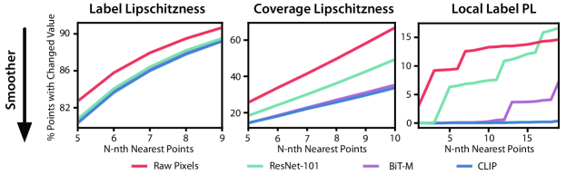
Prompting	F1-score
No Prompt	48.5
Prompt at Beginning	50.2
Prompt at End	52.2

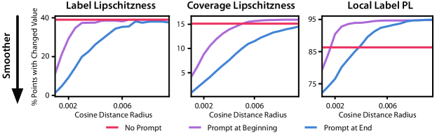
Figure 3: Top: Liger performance and smoothness measurements of CLIP, BiT-M, ResNet-101, and raw pixels as embeddings for Basketball. Bottom: Liger performance and smoothness measurements of no prompting, prompting at beginning, and prompting at end in GPT-3 for Spouse.

Figure 3 reports two additional measurements of smoothness on Basketball and Spouse—coverage Lipschitzness and local label probabilistic Lipschitzness (see Section 4 for the formal definitions). Trends match label Lipschitzness.

To measure label Lipschitzness, the property that $|\Pr(y=1|x)-\Pr(y=1|x^{\prime})|\leq K_{y}\rho(f(x),f(x^{\prime}))$, we observe that

$$|\Pr(y=1|x)-\Pr(y=1|x^{\prime})| =|\mathbb{E}\left[\mathbbm{1}\left\{y=1|x\right\}-\mathbb{E}\left[\mathbbm{1}\left\{y=1|x^{\prime}\right\}\right]\right]$$

$$\leq\mathbb{E}\left[|\mathbbm{1}\left\{y=1|x\right\}-\mathbbm{1}\left\{y=1|x^{\prime}\right\}|\right]$$

$$=\mathbb{E}\left[\mathbbm{1}\left\{y\neq y^{\prime}\right\}\right]=\Pr(y\neq y^{\prime})$$

by Jensen’s inequality. Therefore, we estimate $\Pr(y=y^{\prime})$ on data as an upper bound on label Lipschitzness. We do this by computing the average percentage of points in some local region (defined either by a radius or by nearest neighbors) around a given point where the label is different from that of the given point.

For source Lipschitzness, the sources in practice are unimodal and hence $K_{\lambda}=0$.

For coverage Lipschitzness, we note that $|\Pr(\lambda_{i}\neq 0|x)-\Pr(\lambda_{i}\neq 0|x^{\prime})|\leq\Pr(\mathbbm{1}\left\{\lambda_{i}(x)\neq 0\right\}!=\mathbbm{1}\left\{\lambda_{i}(x)\neq 0\right\})$, so we estimate this probability on data as an upper bound. This is done by computing the average percentage of points that abstain in some local region around a point that has coverage, and vice versa. We average over all sources.

Finally, for local label probabilistic Lipschitzness, we follow Definition 2. For each point in the support of $\lambda_{i}$, we search if there exists a nearby point within radius $r$ (or $k$-th nearest neighbor) such that this nearby point is not in the support and has a label differerent from that of the given point. We compute the percentage of points in the support that satisfy this property. We average over all sources.

To read $K_{y},K_{\lambda,0},M$ from Figure 3, they can each be viewed as the slope of the linear function that upper bounds the smoothness curve. Note that for the curves that appear flat (i.e. no prompt), these constants are very large, as there is an initial sharp increase in the percentage of points with changed value.

F.3 Synthetic Experiments

We evaluate Liger on synthetic data to confirm our insights about 1) how generalization error for $\hat{\Pr}(y|\bm{\lambda},x)$ demonstrates a bias-variance tradeoff depending on the number of partitions, and 2) how additional lift depends on setting the threshold radius based on the original weak source’s accuracy and the embedding’s probabilistic Lipschitzness.

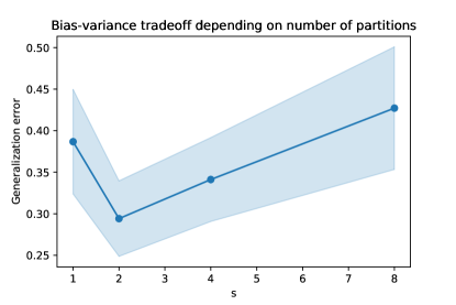
Figure 4: The bias-variance tradeoff in the generalization error based on $s$, the number of partitions used in our approach. When too few partitions are used, the accuracy estimates are not fine-grained and do not sufficiently approximate the true conditional distribution $\Pr(y,\bm{\lambda}|x)$, resulting in large bias. When too many partitions are used, the variance increases due to sampling error on individual partitions.

First, we conduct a synthetic experiment to understand how the number of partitions $s$ controls the bias-variance tradeoff in generalization error of $\hat{\Pr}(y|\bm{\lambda},x)$ (Theorem 1. We generate two sets of canonical parameters and use them in (1) to generate $(y,\bm{\lambda})$ from two different distributions, $\mathcal{P}_{1}$ and $\mathcal{P}_{2}$ over an embedding space. We generate $1000$ points each for $\mathcal{P}_{1}$ and $\mathcal{P}_{2}$ to form datasets $\mathcal{D}_{1}$ and $\mathcal{D}_{2}$, which are then concatenated to form a dataset $\mathcal{D}$ of $2000$ points. We first run Algorithm 1 with $s=1$, which means that we estimate only one set of parameters over $\mathcal{D}$ despite the dataset consisting of two different conditional distributions. We then set $s=2$ and estimate the parameters of $\mathcal{P}_{1}$ and $\mathcal{P}_{2}$ separately over $1000$ points each. Finally, we set $s=4$ and $s=8$ by dividing each of $\mathcal{D}_{1}$ and $\mathcal{D}_{2}$ into $2$ subsets of $500$ points and $4$ subsets of $250$ points, respectively. For each of these, we compute the average cross-entropy loss (over $s$) of our label model. Figure 4 plots how the generalization error changes with the number of partitions $s$. We plot the mean and $95\%$ confidence interval over ten random initializations of canonical parameters and datasets drawn according to them. It demonstrates a bias-variance tradeoff: when $s=1$, we estimate one set of parameters over the entire dataset rather than the two true sets of parameters, and this approach hence does not capture the distinctions in input space among the source accuracies. As a result, a low $s$ results in high bias, contributing to large generalization error. On the other hand, when $s=4$ or $8$, our approach is correctly estimating $\mathcal{D}_{1}$ and $\mathcal{D}_{2}$ separately but is using much less data to do so. This approach has higher sampling error, which worsens variance and contributes to large generalization error.

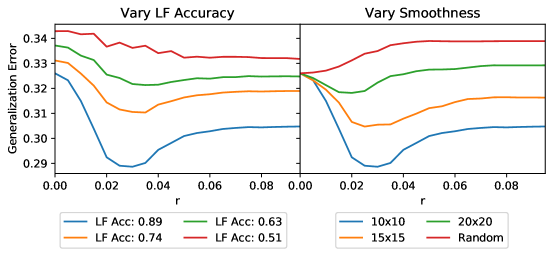
Figure 5: Reduction in generalization error from extending labeling functions of varying accuracies (left), and on embedding spaces of varying smoothness (right). LF refers to a weak source’s labeling function.

Next, we conduct a synthetic experiment to understand how setting the threshold radius of the extended weak source controls improvement in generalization error as a function of the original average source accuracy and the probabilistic Lipschitzness of the FM embedding (Theorem 2). Suppose for simplicity that $s=1$ and that $\Pr(y,\bm{\lambda})$ is modeled the same way as $\Pr(y,\bm{\lambda}|x)$ in (1). This assumption reduces to previous weak supervision settings but allows us to isolate the effect of extending a source. We create an embedding space over $10000$ uniformly sampled points in $[0,1]^{2}$ with a fixed class balance $\Pr(y)$ and $m=3$ labeling functions, where only $\lambda_{1}$ is extended. To understand the impact of a labeling function’s accuracy, we fix a task distribution by assigning $Y$ labels in a $10\times 10$ “checkerboard” pattern and run our algorithm on four versions of $\lambda_{1}$ with varying average accuracies, keeping $\lambda_{1}$’s support consistent. In Figure 5 (left), we extend $\lambda_{1}$ based on $r$ for each of the four versions of the labeling function. This confirms that extending a highly accurate labeling function results in greater generalization lift. To understand the impact of Lipschitzness of the task distribution, we produce four distributions of $Y$ over the embedding space, three of which follow a checkerboard clustering pattern (such that more divisions mean less smoothness), and one that spatially distributes the values of $Y$ at random. For both experiments, we run our approach with threshold radius varying from $0$ to $0.1$ in increments of $0.005$. In Figure 5 (right), each curve represents performance of the same high average accuracy labeling function $(a_{1}=0.89$) over embeddings of varying Lipschitzness. This confirms that the greatest improvement due to an extension occurs for the smoothest embedding. Lastly, both of these graphs illustrate the tradeoff in setting a threshold radius, confirming the theoretical insight that this quantity must be chosen carefully to ensure lift from using $\bar{\lambda}_{1}$ over $\lambda_{1}$.

References

• [1] Weather sentiment: Dataset in crowdflower. https://data.world/crowdflower/weather-sentiment.
• [2] Guillaume Alain and Yoshua Bengio. Understanding intermediate layers using linear classifier probes. arXiv preprint arXiv:1610.01644, 2016.
• [3] Túlio C Alberto, Johannes V Lochter, and Tiago A Almeida. Tubespam: Comment spam filtering on youtube. In 2015 IEEE 14th International Conference on Machine Learning and Applications (ICMLA), 2015.
• [4] Stephen H Bach, Daniel Rodriguez, Yintao Liu, Chong Luo, Haidong Shao, Cassandra Xia, Souvik Sen, Alex Ratner, Braden Hancock, Houman Alborzi, et al. Snorkel drybell: A case study in deploying weak supervision at industrial scale. In Proceedings of the 2019 International Conference on Management of Data, 2019.
• [5] Avrim Blum and Tom Mitchell. Combining labeled and unlabeled data with co-training. In Proceedings of the eleventh annual conference on Computational learning theory. ACM, 1998.
• [6] Benedikt Boecking and Artur Dubrawski. Pairwise feedback for data programming. In Proceedings of NeurIPS 2019 Workshop on Learning with Rich Experience (LIRE), December 2019.
• [7] Rishi Bommasani, Drew A. Hudson, Ehsan Adeli, et al. On the opportunities and risks of foundation models. arXiv preprint arXiv:2108.07258, 2021.
• [8] Tom Brown, Benjamin Mann, Nick Ryder, Melanie Subbiah, Jared D Kaplan, Prafulla Dhariwal, Arvind Neelakantan, Pranav Shyam, Girish Sastry, Amanda Askell, et al. Language models are few-shot learners. Advances in neural information processing systems, 2020.
• [9] Fabian Caba Heilbron, Victor Escorcia, Bernard Ghanem, and Juan Carlos Niebles. Activitynet: A large-scale video benchmark for human activity understanding. In Proceedings of the IEEE Conference on Computer Vision and Pattern Recognition, 2015.
• [10] Salva Rühling Cachay, Benedikt Boecking, and Artur Dubrawski. End-to-end weak supervision. In Advances in Neural Information Processing Systems, 2021.
• [11] Mayee Chen, Benjamin Cohen-Wang, Stephen Mussmann, Frederic Sala, and Christopher Re. Comparing the value of labeled and unlabeled data in method-of-moments latent variable estimation. In Proceedings of The 24th International Conference on Artificial Intelligence and Statistics, 2021.
• [12] Ting Chen, Simon Kornblith, Mohammad Norouzi, and Geoffrey Hinton. A simple framework for contrastive learning of visual representations. In International conference on machine learning. PMLR, 2020.
• [13] David Corney, Dyaa Albakour, Miguel Martinez-Alvarez, and Samir Moussa. What do a million news articles look like? In NewsIR@ECIR, 2016.
• [14] Jacob Devlin, Ming-Wei Chang, Kenton Lee, and Kristina Toutanova. Bert: Pre-training of deep bidirectional transformers for language understanding. arXiv preprint arXiv:1810.04805, 2018.
• [15] Jacob Devlin, Ming-Wei Chang, Kenton Lee, and Kristina Toutanova. BERT: Pre-training of deep bidirectional transformers for language understanding. In Proceedings of the 2019 Conference of the Association for Computational Linguistics, 2019.
• [16] Daniel Y. Fu, Mayee F. Chen, Frederic Sala, Sarah M. Hooper, Kayvon Fatahalian, and Christopher Ré. Fast and three-rious: Speeding up weak supervision with triplet methods. In Proceedings of the 37th International Conference on Machine Learning, 2020.
• [17] Daniel Y. Fu, Will Crichton, James Hong, Xinwei Yao, Haotian Zhang, Anh Truong, Avanika Narayan, Maneesh Agrawala, Christopher Ré, and Kayvon Fatahalian. Rekall: Specifying video events using compositions of spatiotemporal labels. arXiv preprint arXiv:1910.02993, 2019.
• [18] Sonal Gupta and Christopher Manning. Improved pattern learning for bootstrapped entity extraction. In Proceedings of the Eighteenth Conference on Computational Natural Language Learning, 2014.
• [19] Kaiming He, Haoqi Fan, Yuxin Wu, Saining Xie, and Ross Girshick. Momentum contrast for unsupervised visual representation learning. arXiv preprint arXiv:1911.05722, 2019.
• [20] James Hong, Will Crichton, Haotian Zhang, Daniel Y Fu, Jacob Ritchie, Jeremy Barenholtz, Ben Hannel, Xinwei Yao, Michaela Murray, Geraldine Moriba, et al. Analysis of faces in a decade of us cable tv news. In Proceedings of the 27th ACM SIGKDD Conference on Knowledge Discovery & Data Mining, 2021.
• [21] Neil Houlsby, Andrei Giurgiu, Stanislaw Jastrzebski, Bruna Morrone, Quentin De Laroussilhe, Andrea Gesmundo, Mona Attariyan, and Sylvain Gelly. Parameter-efficient transfer learning for nlp. In International Conference on Machine Learning. PMLR, 2019.
• [22] Ahmet Iscen, Giorgos Tolias, Yannis Avrithis, and Ondrej Chum. Label propagation for deep semi-supervised learning. In Proceedings of the IEEE Conference on Computer Vision and Pattern Recognition, pages 5070–5079, 2019.
• [23] Urvashi Khandelwal, Omer Levy, Dan Jurafsky, Luke Zettlemoyer, and Mike Lewis. Generalization through memorization: Nearest neighbor language models. In International Conference on Learning Representations, 2019.
• [24] Ashish Khetan, Zachary C. Lipton, and Anima Anandkumar. Learning from noisy singly-labeled data. In International Conference on Learning Representations, 2018.
• [25] Alexander Kolesnikov, Lucas Beyer, Xiaohua Zhai, Joan Puigcerver, Jessica Yung, Sylvain Gelly, and Neil Houlsby. Big transfer (bit): General visual representation learning. In ECCV, 2020.
• [26] Hunter Lang, Aravindan Vijayaraghavan, and David Sontag. Training subset selection for weak supervision. arXiv preprint arXiv:2206.02914, 2022.
• [27] Brian Lester, Rami Al-Rfou, and Noah Constant. The power of scale for parameter-efficient prompt tuning. In Proceedings of the 2021 Conference on Empirical Methods in Natural Language Processing, 2021.
• [28] Percy Liang, Michael I Jordan, and Dan Klein. Learning from measurements in exponential families. In Proceedings of the 26th annual international conference on machine learning. ACM, 2009.
• [29] Gideon S Mann and Andrew McCallum. Generalized expectation criteria for semi-supervised learning with weakly labeled data. Journal of machine learning research, 2010.
• [30] Arvind Neelakantan, Tao Xu, Raul Puri, Alec Radford, Jesse Michael Han, Jerry Tworek, Qiming Yuan, Nikolas Tezak, Jong Wook Kim, Chris Hallacy, et al. Text and code embeddings by contrastive pre-training. arXiv preprint arXiv:2201.10005, 2022.
• [31] Nicolas Papernot and Patrick McDaniel. Deep k-nearest neighbors: Towards confident, interpretable and robust deep learning. arXiv preprint arXiv:1803.04765, 2018.
• [32] Alec Radford, Jong Wook Kim, Chris Hallacy, Aditya Ramesh, Gabriel Goh, Sandhini Agarwal, Girish Sastry, Amanda Askell, Pamela Mishkin, Jack Clark, et al. Learning transferable visual models from natural language supervision. In International Conference on Machine Learning, 2021.
• [33] Alec Radford, Jeffrey Wu, Rewon Child, David Luan, Dario Amodei, and Ilya Sutskever. Language models are unsupervised multitask learners. OpenAI Blog, 2019.
• [34] Aditya Ramesh, Mikhail Pavlov, Gabriel Goh, Scott Gray, Chelsea Voss, Alec Radford, Mark Chen, and Ilya Sutskever. Zero-shot text-to-image generation. In International Conference on Machine Learning, 2021.
• [35] Alexander Ratner, Stephen H. Bach, Henry Ehrenberg, Jason Fries, Sen Wu, and Christopher Ré. Snorkel: Rapid training data creation with weak supervision. In Proceedings of the 44th International Conference on Very Large Data Bases (VLDB), Rio de Janeiro, Brazil, 2018.
• [36] Alexander Ratner, Braden Hancock, Jared Dunnmon, Frederic Sala, Shreyash Pandey, and Christopher Ré. Training complex models with multi-task weak supervision. In Proceedings of the AAAI Conference on Artificial Intelligence, Jul 2019.
• [37] Olga Russakovsky, Jia Deng, Hao Su, Jonathan Krause, Sanjeev Satheesh, Sean Ma, Zhiheng Huang, Andrej Karpathy, Aditya Khosla, Michael Bernstein, Alexander C. Berg, and Li Fei-Fei. ImageNet Large Scale Visual Recognition Challenge. IJCV, 2015.
• [38] Esteban Safranchik, Shiying Luo, and Stephen H Bach. Weakly supervised sequence tagging from noisy rules. In Thirty-Fourth AAAI Conference on Artificial Intelligence, 2020.
• [39] Frederic Sala, Paroma Varma, Jason Fries, Daniel Y. Fu, Shiori Sagawa, Saelig Khattar, Ashwini Ramamoorthy, Ke Xiao, Kayvon Fatahalian, James Priest, and Christopher Ré. Multi-resolution weak supervision for sequential data. In Advances in Neural Information Processing Systems 32, 2019.
• [40] Ying Sheng, Nguyen Ha Vo, James B. Wendt, Sandeep Tata, and Marc Najork. Migrating a privacy-safe information extraction system to a software 2.0 design. In Proceedings of the 10th Annual Conference on Innovative Data Systems Research, 2020.
• [41] Jake Snell, Kevin Swersky, and Richard Zemel. Prototypical networks for few-shot learning. In Advances in neural information processing systems, pages 4077–4087, 2017.
• [42] Shingo Takamatsu, Issei Sato, and Hiroshi Nakagawa. Reducing wrong labels in distant supervision for relation extraction. In Proceedings of the 50th Annual Meeting of the Association for Computational Linguistics: Long Papers-Volume 1. Association for Computational Linguistics, 2012.
• [43] Ruth Urner and Shai Ben-David. Probabilistic lipschitzness a niceness assumption for deterministic labels. In Learning Faster from Easy Data-Workshop@NIPS, 2013.
• [44] Paroma Varma, Frederic Sala, Ann He, Alexander Ratner, and Christopher Re. Learning dependency structures for weak supervision models. In Proceedings of the 36th International Conference on Machine Learning, 2019.
• [45] Shuohang Wang, Yang Liu, Yichong Xu, Chenguang Zhu, and Michael Zeng. Want to reduce labeling cost? GPT-3 can help. In Findings of the Association for Computational Linguistics: EMNLP 2021, pages 4195–4205, Punta Cana, Dominican Republic, November 2021. Association for Computational Linguistics.
• [46] Eric Zhan, Stephan Zheng, Yisong Yue, Long Sha, and Patrick Lucey. Generating multi-agent trajectories using programmatic weak supervision. In 7th International Conference on Learning Representations, ICLR, 2019.
• [47] Jieyu Zhang, Yue Yu, Yinghao Li, Yujing Wang, Yaming Yang, Mao Yang, and Alexander Ratner. Wrench: A comprehensive benchmark for weak supervision. In Thirty-fifth Conference on Neural Information Processing Systems Datasets and Benchmarks Track (Round 2), 2021.