Spin-induced scalarization and magnetic fields

Abstract

In the presence of certain non-minimal couplings between a scalar field and the Gauss-Bonnet curvature invariant, Kerr black holes can scalarize, as long as they are spinning fast enough. This provides a distinctive violation of the Kerr hypothesis, occurring only for some high spin range. In this paper we assess if strong magnetic fields, that may exist in the vicinity of astrophysical black holes, could facilitate this distinctive effect, by bringing down the spin threshold for scalarization. This inquiry is motivated by the fact that self-gravitating magnetic fields, by themselves, can also promote “spin-induced” scalarization. Nonetheless, we show that in the vicinity of the horizon the effect of the magnetic field $B$ on a black hole of mass $M$, up to $BM\lesssim 1$, works against spin-induced scalarization, requiring a larger dimensionless spin $j$ from the black hole. A geometric interpretation for this result is suggested, in terms of the effects of rotation $vs.$ magnetic fields on the horizon geometry.

I Introduction

The prospect of testing the Kerr hypothesis is now more realistic than ever. Are all black holes (BHs) in the astrophysical mass range ($\sim$ 1 to $10^{10}$ $M_{\odot}$), and for all spins really well described by the Kerr metric Kerr (1963)? The unprecedented access to strong gravity data, both through gravitational waves Abbott et al. (2016a, b, 2017a, 2017b, 2020, 2021) and from electromagnetic observations Abuter et al. (2020); Akiyama et al. (2019) will provide hints, or even clear answers, about this central question in strong gravity.

Amongst the Kerr hypothesis violating models, a sub-class still accommodates the Kerr solution of vacuum General Relativity (GR), but questions the universality of the hypothesis. Such models typically introduce new scales; these define a mass/spin range in which BHs can become non-Kerr, whereas Kerr BHs remain as the solution of the model in a complementary range.

A concrete illustration of this sub-class of models occurs via the mechanism of spontaneous scalarization. Originally proposed in scalar-tensor theories and for neutron stars Damour and Esposito-Farese (1993), the spontaneous scalarization of vacuum GR BHs occurs in extended scalar-tensor models, wherein a real scalar field with a canonical kinetic term, requiring no mass or self-interactions, minimally couples to the Gauss-Bonnet (GB) quadratic curvature invariant, via a coupling $\eta f(\phi)$, where $\eta$ is a coupling constant and $f(\phi)>0$ a coupling function. We are then led to consider electrovacuum GR augmented by such a scalar field and such a GB curvature correction: an Einstein-Maxwell-scalar-GB (EMsGB) model, $cf.$ action (1) below.

Depending on the sign of the coupling function, $\eta$, the scalarization has different triggers. For $\eta>0$ Schwarzschild BHs with mass $M$ scalarize, as long as $M/\sqrt{\eta}$ is small enough Silva et al. (2018); Doneva and Yazadjiev (2018a); Antoniou et al. (2018). Adding spin to the Schwarzschild BH actually quenches the effects of the scalarization Cunha et al. (2019); Collodel et al. (2020), albeit alleviating slightly the constraint on $M/\sqrt{\eta}$. In this case scalarization, which is due to a tachyonic instability, is promoted by spacetime regions wherein the GB curvature invariant is (sufficiently) positive. Following Herdeiro et al. (2021a) we call this GB⁺ scalarization.

For $\eta<0$, on the other hand, the tachyonic instability is promoted by spacetime regions where the GB curvature invariant is negative, hereafter dubbed GB^- scalarization. For vacuum GR BHs - $i.e.$ the Kerr family - this occurs for dimensionless spin $j>0.5$. Since the negative GB patches occur in the strong gravity region neighbouring the horizon, they trigger scalarization immediately as they appear. Thus Kerr BHs with $j>0.5$ undergo scalarization in these models, which was dubbed “spin-induced” scalarization Dima et al. (2020). Spin-induced scalarization can thus be regarded as a concrete example of GB^- scalarization. The corresponding scalarized BHs were constructed in Herdeiro et al. (2021b); Berti et al. (2021).

GB^- scalarization can also be triggered by other sources rather than BH spin. Of particular interest for us is the case of self-gravitating magnetic fields. In electrovacuum GR, these are described by the Melvin magnetic Universe Melvin (1964). It is known that such universes have regions with a negative GB invariant Brihaye et al. (2021) and can thus promote GB^- scalarization. One may then ask if the presence of a strong magnetic field in the vicinity of a spinning BH may facilitate GB^- (aka, in this context, spin-induced) scalarization, promoting it for $j<0.5$. The goal of this paper is to answer this question, showing that this is not the case.

Astrophysical BHs are thought to be neutrally charged, due to, $e.g.$ quantum discharge Gibbons (1975) and electron-positron pair production Blandford and Znajek (1977). The inclusion of magnetic fields in BH environments is, nonetheless, well motivated. There is in fact observational evidence of astrophysical magnetic fields; elongated sources present in radio-relics Kierdorf et al. (2017) – diffuse radio sources in galaxy clusters Kempner et al. (2003) – are an example. Furthermore, there are known observations supporting the existence of BHs immersed in magnetic backgrounds, as the case of the presence of the magnetar SGR J$1745-29$ in the vicinity of Sagittarius A^∗ Mori et al. (2013); Kennea et al. (2013); Eatough et al. (2013); Olausen and Kaspi (2014), or the strong magnetic fields in the proximity of the event horizon of M87^∗ Akiyama et al. (2021).

In this work, we investigate the effects on GB^- scalarization due to magnetic fields around spinning BH spacetimes, in the EMsGB model. Our strategy will be to consider spinning BHs in Melvin Universes in electrovacuum, investigating the impact of the magnetic field on the regions where the GB invariant becomes negative. Although Melvin Universes are irrealistic to describe globally astrophysical BHs, due to the non-trivial asymptotics, one may argue that in the vicinity of the BH, where the relevant physics that we are investigating is developing, they capture, approximately, the appropriate physics in the case of poloidal magnetic fields.

This paper is organized as follows. In Sec. II the EMsGB model is described and its relevant equations are shown. In Sec. III we review the relevant electrovacuum GR solutions describing a BH immersed in magnetic environments. The main analysis and results of this paper are presented in Sec. IV where we show how and when the necessary condition for ${\rm GB}^{-}$ scalarization can be satisfied in magnetized BH spacetimes. Finally, conclusions are provided in Sec.V.

II Theoretical setup

The action of the EMsGB model is

$$\frac{1}{16\pi}\int d^{4}x\sqrt{-g}\left[R-F_{\mu\nu}F^{\mu\nu}-\frac{1}{2}\left(\nabla\phi\right)^{2}+\frac{\eta}{4}\mathfrak{f}(\phi)\mathcal{R}_{\rm GB}\right]$$ (1)

where $F_{\mu\nu}$ is the usual Faraday tensor, defined by means of the derivatives of the electromagnetic 4-potential $F_{\mu\nu}=\nabla_{\mu}A_{\nu}-\nabla_{\nu}A_{\mu}$; $\eta$ is the dimensionful coupling constant of the theory and $\mathfrak{f}\left(\phi\right)>0$ is a generic coupling function between the scalar field and the GB invariant $\mathcal{R}_{\rm GB}$, that is given by

$$\mathcal{R}_{\rm GB}\equiv R^{2}-4R_{\mu\nu}R^{\mu\nu}+R_{\mu\nu\alpha\beta}R^{\mu\nu\alpha\beta}\,,$$ (2)

with $R\left(R_{\mu\nu}\right)$ being the Ricci scalar (tensor) and $R_{\mu\nu\alpha\beta}$ the Riemann tensor. If not specified otherwise we use geometrized units in which $G=1=c$. Varying the action with respect to the dynamical fields one gets the coupled EMsGB system of equations,

$$\square\phi =-\frac{\eta}{4}\frac{\partial\mathfrak{f}\left(\phi\right)}{\partial\phi}\mathcal{R}_{\rm GB}\,,$$ (3)

$$\nabla_{\mu}F^{\mu\nu} =0\,,$$ (4)

$$R_{\mu\nu}-\frac{1}{2}g_{\mu\nu}R =T_{\mu\nu}^{\left(F\right)}+\frac{1}{2}T_{\mu\nu}^{\left(\Phi\right)}-\frac{1}{8}\eta\,T_{\mu\nu}^{\left(\mathcal{R}_{\rm GB}\right)}\,,$$ (5)

where

$$T_{\mu\nu}^{\left(\phi\right)} =\partial_{\mu}\phi\partial_{\nu}\phi-\frac{1}{2}g_{\mu\nu}\partial_{\alpha}\phi\partial^{\alpha}\phi\,,$$ (6)

$$T_{\mu\nu}^{\left(F\right)} =2F_{\mu\alpha}F_{\nu}^{\,\,\alpha}-\frac{1}{2}F_{\alpha\beta}F^{\alpha\beta}g_{\mu\nu}\,,$$ (7)

$$T_{\mu\nu}^{\left(\mathcal{R}_{\rm GB}\right)} =16R^{\alpha}_{(\mu}\mathcal{C}_{\nu)\beta}+8\mathcal{C}^{\alpha\beta}\left(R_{\mu\alpha\nu\beta}-g_{\mu\nu}R_{\alpha\beta}\right)$$

$$\quad\,-8\mathcal{C}G_{\mu\nu}-4R\mathcal{C}_{\mu\nu}\,,$$ (8)

with

$$\mathcal{C}_{\mu\nu}=\nabla_{\mu}\nabla_{\nu}\mathfrak{f}\left(\phi\right)=\mathfrak{f}^{\prime}\nabla_{\mu}\nabla_{\nu}\phi+\mathfrak{f}^{\prime\prime}\nabla_{\mu}\phi\nabla_{\nu}\phi\,,$$ (9)

$\mathcal{C}=g^{\alpha\beta}\mathcal{C}_{\alpha\beta}$, “prime” denotes derivative with respect to the argument and parentheses in the subscripts indicate symmetrization.

We shall be interested in models for which

$$\frac{\partial\mathfrak{f}}{\partial\phi}\left(\phi=0\right)=0\ ,$$ (10)

such that $\phi=0$ together with any electrovacuum GR solution, is a solution of this model. Moreover, if $\eta<0$ and

$$\frac{\partial^{2}\mathfrak{f}}{\partial\phi^{2}}\left(\phi=0\right)>0\ ,$$ (11)

tachyonic perturbations exist in regions where $\mathcal{R}_{\rm GB}<0$. This is the trigger of GB^- scalarization. The simplest GB coupling function obeying these conditions, which is also the small $\phi$ approximation of a generic analytic coupling function obeying these conditions, is a quadratic function:

$$\mathfrak{f}\left(\phi\right)=\phi^{2}/2\,.$$ (12)

Indeed, in linear perturbation theory, Eq. (3), together with Eq. (12), takes the simple form,

$$\left(\square-\mu^{2}_{\rm eff}\right)\phi=0\,,$$ (13)

where

$$\mu^{2}_{\rm eff}=-\frac{\eta}{4}\mathcal{R}_{\rm GB}\,.$$ (14)

When Eq. (14) takes negative values, the scalar field acquires a tachyonic mass. If there exists a region in which this condition is met, then a tachyonic instability potentially occurs Hod (2020). A simple calculation shows that for Kerr BH this happens if $j>0.5$ Dima et al. (2020). This triggers spin-induced (or GB^-) scalarization.

III Magnetized solutions

Under the condition (10), the system (3)-(5) admits a consistent truncation corresponding to the Einstein-Maxwell (EM) theory, together with $\phi=0$. Thus electrovacuum GR solutions and a trivial scalar field are admissible solutions of the full set of equations of motion. We now describe the EM solutions describing BHs in magnetic Universes.

The non-singular Melvin Universe Melvin (1964) is an exact solution of EM theory that represents a cylindrically symmetric, non-singular, non-asymptotically flat, clump of self-gravitating magnetic flux lines in equilibrium. It is given by

$$ds^{2}=\Lambda^{2}\left(-dt^{2}+d\rho^{2}+dz^{2}\right)+\Lambda^{-2}\rho^{2}d\varphi^{2}\,,$$ (15)

written in cylindrical coordinates ($t,\rho,z,\varphi$). The function $\Lambda$ introduces the strength of the magnetic field $B$, which is the only parameter describing the solution, and it only depends on the radial cylindrical coordinate:

$$\Lambda=1+\frac{1}{4}B^{2}\rho^{2}\,.$$ (16)

Many properties of this magnetic Universe and generalizations thereof have been studied over the years - see $e.g$ Gibbons and Herdeiro (2001); Tseytlin (1995); Bambi et al. (2015); Garfinkle and Glass (2011); Kastor and Traschen (2021); Gutperle and Strominger (2001); Costa et al. (2001); Junior et al. (2021a, b).

It is possible to add a neutral BH, with horizon mass $M$, inside the Melvin magnetic Universe described by Eq. (15). Remarkably, an exact 2-parameter solution to such problem exists, which reduces to the Schwarzschild spacetime for $B=0$, and to the Melvin magnetic Universe for $M=0$. In usual spherical polar coordinates ($t,r,\theta,\varphi$), the metric of such a Schwarzschild-Melvin BH spacetime takes the simple form,

$$ds^{2}=\Lambda^{2}(-fdt^{2}+f^{-1}dr^{2}+r^{2}d\theta^{2})+\Lambda^{-2}r^{2}\sin^{2}\theta d\varphi^{2}\,,$$ (17)

where $f=1-2M/r$, with $M$ representing the mass of the spacetime Radu (2002) and $\Lambda$ is now given by

$$\Lambda=1+\frac{1}{4}B^{2}r^{2}\sin^{2}\theta\,.$$ (18)

Further increasing the complexity, it is also possible to add a charge parameter $Q$ to the previous BH in the Melvin magnetic Universe Ernst (1976). An exact 3-parameter solution to such problem exists, which reduces to the Reissner-Nordström (RN) solution for $B=0$, to the previous Schwarzschild-Melvin spacetime for $Q=0$ and to the Melvin magnetic Universe for $M=0=Q$ Ernst (1976). The metric of such RN-Melvin BH is given by

$$ds^{2} =\lvert\Lambda\rvert^{2}(-\tilde{f}dt^{2}+\tilde{f}^{-1}dr^{2}+r^{2}d\theta^{2})$$

$$\quad\,+\lvert\Lambda\rvert^{-1}r^{2}\sin^{2}\theta\left(d\varphi-\tilde{\omega}dt\right)^{2}\,,$$ (19)

where $\tilde{f}=1-2M/r+Q^{2}/r^{2}$, with $Q$ being the electric charge of the BH and

$$\Lambda =1+\left(1/4\right)B^{2}\left(r^{2}\sin^{2}+Q^{2}\cos^{2}\theta\right)-iBQ\cos\theta\,,$$ (20)

$$\tilde{\omega} =-2BQr^{-1}+B^{3}Qr+\left(1/2\right)B^{3}Q^{3}r^{-1}$$

$$\quad\,-\left(1/2\right)B^{3}Qr^{-1}\left(r^{2}-2Mr+Q^{2}\right)\sin^{2}\theta+{\rm cst}\,.$$ (21)

The novel feature of the RN-Melvin spacetime is that, due to the non-trivial Poynting vector, resulting from the existence of an electric charge inside a magnetic field, the spacetime becomes stationary, rather than static, despite the $B=0$ limit being static. Loosely speaking, a RN BH in a Melvin Universe starts to spin. See, $e.g.$ Santos and Herdeiro (2021) for the full solution, including the gauge field.

It is also possible to add a Kerr, or Kerr-Newman (KN) BH inside the Melvin magnetic Universe, as long as the symmetry axes are aligned. Such solution was first analysed in a linear setup by Wald Wald (1974). Soon after, the fully non-linear rotating BH solution containing back-reacting magnetic fields was determined in the seminal works of Ernst Ernst (1976), and Ernst and Wild Ernst and Wild (1976). Generalizations and extensions of Ref. Ernst (1976) have been attained (see Budinova et al. (2000); Bičák et al. (2007) for detailed overviews and Gibbons et al. (2014); Astorino et al. (2016); Booth et al. (2015); Astorino (2015, 2017) for details on their thermodynamic properties).

The full metric of a KN-Melvin BH is displayed in detail in Ref. Gibbons et al. (2013), where it has been obtained from magnetizing a seed KN BH through solution-generating techniques, developed by Harrison Harrison (1968). The resulting spacetime is an axially symmetric geometry that depends on the $\left\{r,\theta\right\}$ spacetime components. Furthermore, in general, it depends on the parameters of the seed KN BH considered before the magnetization procedure, $i.e.$ $\left\{M,J,q\right\}$ and on the magnetic field parameter $B$ introduced by the procedure. The (rather) lengthy geometry of a KN-Melvin BH it is given explicitly in Appendix B of Ref. Gibbons et al. (2013). For simplicity, we discuss here only its main properties without displaying all its components,

$$ds^{2} =H\left[-fdt^{2}+R^{2}\left(\frac{dr^{2}}{\Delta}+d\theta^{2}\right)\right]$$

$$\quad\,+\frac{\Sigma\sin^{2}\theta}{HR^{2}}\left(d\varphi-\omega dt\right)^{2}\,,$$ (22)

$$A_{\mu} =\left(\Phi_{0}-\omega\Phi_{3},0,0,\Phi_{3}\right)\,,$$ (23)

where

$$R^{2} =r^{2}+a^{2}\cos^{2}\theta\,$$

$$\Delta =\left(r^{2}+a^{2}\right)-2Mr+q^{2}\,,$$

$$\Sigma =\left(r^{2}+a^{2}\right)^{2}-a^{2}\Delta\sin^{2}\theta\,,$$

$$f =R^{2}\Delta\Sigma^{-1}\,,$$ (24)

where $a$ is defined through the usual KN BH angular momentum ($a\equiv J/M$) and $H,\omega,\Phi_{0},\Phi_{3}$ are all complicated functions of $\left(r,\theta\right)$ and $\left(M,a,q,B\right)$, given, respectively, in Eqs. (B.5), (B.8), (B.15) and (B.17) of Gibbons et al. (2013). To ensure the validity of our findings, we have verified that the metric and vector potential in Eqs. (III)-(23) satisfy the Einstein-Maxwell system and that correctly tend to the KN geometry when $B=0$.

The KN-Melvin geometry has for a long time been thought to tend asymptotically to the Melvin Universe. Instead, only relatively recently Gibbons et al. (2013), it has been shown that this is the case only if

$$q=-aMB\,.$$ (25)

The condition in Eq. (25) ensures that the ergoregion surrounding the KN-Melvin BH does not extend to spatial infinity, and we are going to restrict to such case in the following analysis of the KN-Melvin, that we call Case I.

Despite the asymptotic property that distinguishes it, Case I has the caveat that the seed BH (in the magnetization procedure) is already electrically charged and one may object that this is not the ideal to try to describe an astrophysical system wherein the BH is expected to have negligible electric charge. Thus, we also consider the Kerr-Melvin solution as Case II in which the seed BH has no electric charge, in which case $q=0$ and condition (25) is not imposed. As we shall see below, the main conclusions will be common to both Case I and Case II.

In preparation for the next section, let us specify the horizons’ positions in Eq. (III). As usual, they are located at the roots of $1/g_{rr}$. Following the notation of Gibbons et al. (2013), and restricting to Case I, one can find that

$$r_{\pm}=\left(1\pm\tilde{\varepsilon}\right)M\,,$$ (26)

where $\tilde{\varepsilon}^{2}=1-\varepsilon^{2}$, and $\varepsilon$ is defined through,

$$\varepsilon\equiv\frac{a}{M}\sqrt{1+B^{2}M^{2}}\ ,\qquad{\rm with}\ \ \ 0\leqslant\varepsilon\leqslant 1\,.$$ (27)

From Eq. (27) it is clear that if $BM\neq 0$, since $0\leqslant j=a/M\leqslant 1$, KN BH with a sufficiently large value of $j$ cannot support external magnetic fields without developing naked singularities, hence they are non-physical. For Case II instead, the event horizon location does not differ from the well-known Kerr case.

IV Scalarization and magnetized spacetimes

In the previous section we have set the stage to analyse Case I and Case II of KN-Melvin spacetimes. Now, let us analyse the necessary condition that triggers the scalarization instability.

As mentioned earlier, the effect of a self-gravitating magnetic field, per se, could support the GB^- instability. In a Schwarzschild-Melvin BH spacetime, near the horizon the GB invariant has the form,

$$\mathcal{R}_{\rm GB}\left(r\sim 2M\right)=\left({4M^{4}\left(\left(BM\sin\theta\right)^{2}+1\right)^{8}}\right)^{-1}\times$$

$$\bigg{[}3\left[\left(BM\sin\theta\right)^{8}-2\left(BM\sin\theta\right)^{4}+\left(\left(BM\right)^{4}\sin^{2}\left(2\theta\right)-1\right)^{2}\right]$$

$$\quad\;+24\cos^{2}\theta\left(\left(BM\right)^{8}\sin^{6}\theta-\left(BM\right)^{6}\sin^{4}\theta+\left(BM\right)^{2}\right)$$

$$\quad\;+16\left(BM\right)^{4}\cos^{4}\theta\left(1-6\left(BM\right)^{2}\sin^{2}\theta\right)\bigg{]}\,.$$ (28)

Thus, there exists a range of angles $\theta$ such that $\mathcal{R}_{\rm GB}$ assumes negative values whenever,

$$BM>0.971\,.$$ (29)

Therefore, for sufficiently large $BM$ the necessary condition for scalarization (near the BH) is obeyed. For the Kerr BH the onset of the instability coincides with the emergence of a negative GB spacetime region (near the horizon). Thus the necessary condition for GB^- scalarization is also sufficient. Assuming a similar scenario in the presence of the magnetic field, the above calculation provides us with an estimate for the onset of ${\rm GB}^{-}$ scalarization in static spacetimes; restoring physical units, we obtain,

$$B\simeq 2\times 10^{13}\,{\rm G}\left(\frac{4\times 10^{6}M_{\odot}}{M}\right)\,,$$ (30)

where we normalized to the mass of Sagittarius A^∗. The above number above is relatively high, but still within the regime of the highest magnetic fields ever measured Olausen and Kaspi (2014).

For what concerns KN-Melvin BHs, a similar analysis can be done. However, given the size of Eq. (III), it is impractical to show the full form of $\mathcal{R}_{\rm GB}$ here. Therefore, in Fig. 1 we display the regions where $\mathcal{R}_{\rm GB}$ becomes negative for at least one value of $\theta$, in a $\left\{BM,j\equiv J/M^{2}\right\}$ phase-space, for both Case I (left) and Case II (right).

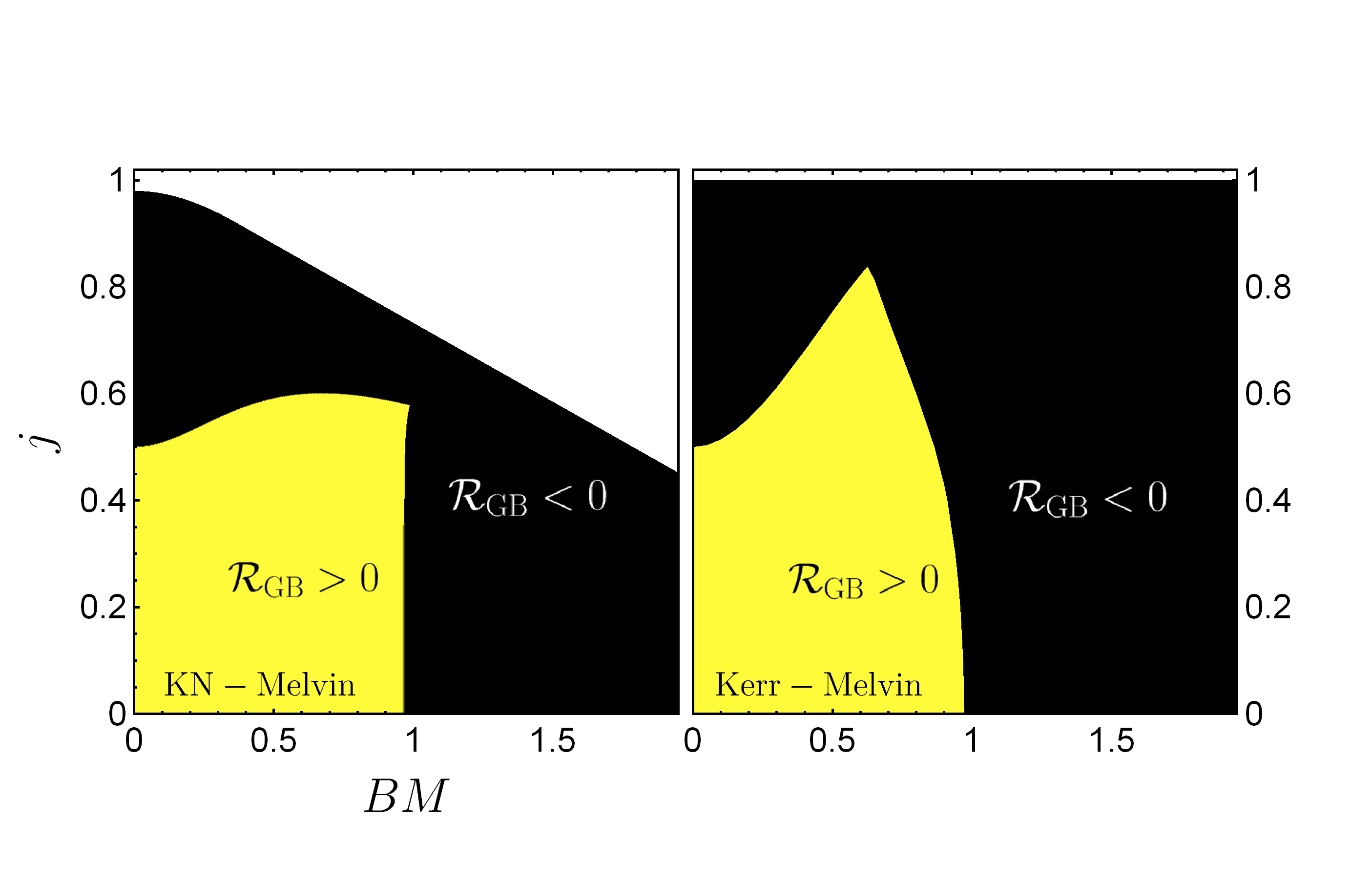
Figure 1: Analysis of the sign of the GB invariant on the BH horizon for Case I (left panel) and Case II (right panel). The yellow region represents the domain in the $\left\{BM,j\right\}$ phase-space, where the GB invariant takes positive values for any azimuthal angle $\theta$ at the BH horizon. For black regions, on the other hand, there is at least one value of $\theta$ such that $\mathcal{R}_{\rm GB}$ takes negative values. In the left panel, no KN-Melvin BHs are allowed in the top white region of the phase-space. That is due to the requirement of the existence of an event horizon for a KN-Melvin BH, $cf.$ eq. (27).

In the limit where $j\rightarrow 0$, we get the expected threshold for Schwarzschild-Melvin BHs (see Eq. (IV)). Conversely, for small $B$, the threshold to have a negative $\mathcal{R}_{\rm GB}$ near the horizon is obtained for $j\geqslant 0.5$, as expected. However, starting from $BM=0,\,j=0.5$ and increasing the magnetic field, the necessary condition to have unstable static scalar perturbations is satisfied for larger values of $j$, compared to the Kerr BH limit. This perhaps surprising result shows that the effect of adding an external magnetic field to a Kerr BH is not making the scalarization process easier to happen, instead, it leads to GR solutions that are more stable than their non-magnetized counterparts, regardless of the case considered. A similar result is evident also considering slowly-rotating BHs in a neighborhood of the scalarization threshold of Schwarzschild-Melvin BH. Ultimately, Fig. 1 indicates that rotation and magnetic fields possess different and somehow opposing roles near the horizon, although they may both trigger the instability of KN-Melvin spacetimes separately. These results can be straightforwardly generalized to bosonic fields with non-zero spins.

An important remark is in order concerning physical quantities. The mass and angular momentum parameters in Fig. 1 refers to the seed Kerr (or KN) BH ones. A definition of mass and angular momentum in spacetime with non-flat asymptotics quantities – through Komar integrals, for instance – may be difficult to obtain. Yet it has been shown Astorino et al. (2016) that in the case of KN-Melvin BHs, it is possible to use the so-called canonical integrability method Barnich and Brandt (2002); Barnich (2003); Barnich and Compere (2008) to obtain the physical quantities for such spacetimes. Following Ref. Astorino et al. (2016), we have checked that, using the physical BH parameters, the qualitative behaviour seen is similar to that in the left panel of Fig. 1; $i.e.$ it is consistent with using the seed parameters.

IV.1 A geometrical interpretation

As previously stated, the necessary condition to undergo tachyonic instability concerns the 4-dimensional $\mathcal{R}_{\rm GB}$ invariant. However, let us try to interpret the results of Fig. 1 inspecting the horizon (2D) geometry of the KN-Melvin geometry.

Previous studies have shown that both rotation and the inclusion of magnetic fields deform the geometry of the BH external horizon Smarr (1973); Wild and Kerns (1980); Kulkarni and Dadhich (1986); Costa et al. (2009); Gibbons et al. (2009); Junior et al. (2021a). Concretely, the effect of rotation turns the Kerr horizon into an oblate spheroid (compared to the spherical Schwarzschild horizon), perpendicularly to the angular momentum of the rotating BH ($z-$axis). The larger the rotation the more oblate becomes the horizon shape. In order to visualize the BH horizon, one might embed it isometrically in Euclidean 3-dimensional space. Notably, for Kerr BHs, such procedure is possible only for relatively slow BHs (precisely, up to $a=\sqrt{3}/2M$).

Likewise, the horizon structure of a Schwarzschild-Melvin BH is deformed in comparison to the static BH case. However, conversely to the Kerr case, the horizon geometry is deformed in the same direction as the external magnetic field, making it a prolate spheroid. As expected, a larger $BM$ corresponds to a more deformed horizon structure. In order to visualize the horizon structure of KN-Melvin BHs, we followed the work of Smarr Smarr (1973), but including an external magnetic field. Our results are shown in Fig. 2: the inclusion of magnetic fields counter-balance the effects of rotation, yielding a more spherical horizon shape to spinning and magnetized spacetimes. This provides some insight on how the rotation and magnetic field have a conflicting geometric effect, once a KN BH is placed in the external magnetic field.

Figure 2: BH horizon isometric embeddings in Euclidean 3-dimensional space ($x-z$ sections) for different values of $\left\{BM,j\right\}$. As rotation increases, the horizon becomes oblate (perpendicularly to the axis of rotation). Increasing $B$ instead elongates the horizon along the $z-$direction (prolate). In the case where both rotating and magnetic fields are present, the structure resembles the static case.

V Conclusions

A paradigmatic mechanism that leads to new field configurations is given by “spontaneous scalarization”. This process has been discovered in the framework of scalar-tensor theories Damour and Esposito-Farese (1993), where a scalar field, coupled to gravity, triggers a tachyonic instability, leading to stars with non-trivial scalar charges. These compact stars are said to be scalarized Damour and Esposito-Farese (1992). A similar scalarization mechanism might also happen in vacuum BH spacetimes, when non-trivial couplings between a scalar and (higher-order) curvatures are present Silva et al. (2018); Doneva and Yazadjiev (2018a); Witek et al. (2019); Silva et al. (2019); Minamitsuji and Ikeda (2019a); Doneva et al. (2019); Fernandes et al. (2019); Minamitsuji and Ikeda (2019b); Cunha et al. (2019); Andreou et al. (2019); Ikeda et al. (2019); Annulli (2021). In these theories, scalarized BHs differ from the Kerr family because some of the assumption of the above-mentioned no-hair theorems cease to be valid.

Recent works in the context of Einstein-scalar-Gauss-Bonnet theory have shown that both static and fastly spinning BHs might suffer from tachyonic instabilities Silva et al. (2018); Doneva and Yazadjiev (2018a); Dima et al. (2020), depending on the sign of the GB curvature invariant ($\mathcal{R}_{\rm GB}$). Further details on the properties of rotating and non-rotating scalarized BHs in EsGB have been obtained, among others, in Refs. Blázquez-Salcedo et al. (2018); Collodel et al. (2020); Berti et al. (2021); Pierini and Gualtieri (2021). ${\rm GB}^{-}$ scalarization is not a unique feature of rotating solutions, as recently shown by Ref. Herdeiro et al. (2021a) for charged BH in EMsGB theory. In fact, even object solely formed by magnetic fields, as the Melvin Universe Melvin (1964), might lead to magnetic-induced scalarization Brihaye et al. (2021).

Magnetic fields are ubiquitous in nature. Their impact on BHs, and particles around them, can be crucial in the current GW astronomy era. There are in fact known stars which encompass magnetic fields up to $10^{16}{\rm G}$ Olausen and Kaspi (2014). The interaction of such magnetars and BHs might lead to unexpected and intriguing new phenomena. Simultaneously, it is fundamental as well to enlarge our predictive power, searching for extra BH charges coming from modification of GR. Hence, in the context of EMsGB theories, in this paper we have shown that astrophysical BHs tend to be more stable, once magnetic fields are added to Kerr spacetimes. The two effects of rotation and magnetic field are therefore substantially different in the near horizon region of KN-Melvin BHs, at least up to $BM\sim 1$.

A thorough analysis of scalar perturbations in such theory might be possible. Practically this means solving for static scalar perturbations around a KN-Melvin BH. This study would provide the exact values for the onset of the instability in the $BM$ and $j$ phase-space. However, going through this path raises important issues. In fact, as previously mentioned, a cutoff in the magnetic field would be needed in order to ensure asymptotic flatness, and this procedure introduces ambiguities. Furthermore, the results exhibited in Fig. 1 clearly show that adding a magnetic field is not enhancing the scalarization process of KN BH thus making the result in this paper clear: spin-induced scalarization is not facilitated by magnetic fields, at least poloidal ones that can be approximately described, near the horizon, by the Melvin magnetic Universe, as long as $BM\lesssim 1$.

Acknowledgements

We thank Haroldo Lima Junior for important feedback. This work is supported by the Center for Research and Development in Mathematics and Applications (CIDMA) through the Portuguese Foundation for Science and Technology (FCT - Fundação para a Ciência e a Tecnologia), references UIDB/04106/2020, UIDP/04106/2020. LA is supported by the University of Aveiro through a PostDoc research grant, reference BIPD/UI97/9854/2021. We acknowledge support from the projects PTDC/FIS-OUT/28407/2017, CERN/FISPAR/0027/2019 and PTDC/FIS-AST/3041/2020. This work has further been supported by the European Union’s Horizon 2020 research and innovation (RISE) programme H2020-MSCA-RISE-2017 Grant No. FunFiCO-777740.

References

- Kerr (1963) R.P. Kerr, Phys. Rev. Lett. 11, 237 (1963).
- Abbott et al. (2016a) B.P. Abbott et al. (Virgo, LIGO Scientific), Phys. Rev. Lett. 116, 061102 (2016a), arXiv:1602.03837.
- Abbott et al. (2016b) B.P. Abbott et al. (Virgo, LIGO Scientific), Phys. Rev. Lett. 116, 241103 (2016b), arXiv:1606.04855.
- Abbott et al. (2017a) B.P. Abbott et al. (VIRGO, LIGO Scientific), Phys. Rev. Lett. 118, 221101 (2017a), [Erratum: Phys.Rev.Lett. 121, 129901 (2018)], arXiv:1706.01812.
- Abbott et al. (2017b) B. Abbott et al. (LIGO Scientific, Virgo), Phys. Rev. Lett. 119, 141101 (2017b), arXiv:1709.09660.
- Abbott et al. (2020) R. Abbott et al. (LIGO Scientific, Virgo), Phys. Rev. Lett. 125, 101102 (2020), arXiv:2009.01075.
- Abbott et al. (2021) R. Abbott et al. (LIGO Scientific, VIRGO), (2021), arXiv:2108.01045.
- Abuter et al. (2020) R. Abuter et al. (GRAVITY), Astron. Astrophys. 636, L5 (2020), arXiv:2004.07187.
- Akiyama et al. (2019) K. Akiyama et al. (Event Horizon Telescope), Astrophys. J. Lett. 875, L1 (2019), arXiv:1906.11238.
- Damour and Esposito-Farese (1993) T. Damour and G. Esposito-Farese, Phys. Rev. Lett. 70, 2220 (1993).
- Silva et al. (2018) H.O. Silva, J. Sakstein, L. Gualtieri, T.P. Sotiriou, and E. Berti, Phys. Rev. Lett. 120, 131104 (2018), arXiv:1711.02080.
- Doneva and Yazadjiev (2018a) D.D. Doneva and S.S. Yazadjiev, Phys. Rev. Lett. 120, 131103 (2018a), arXiv:1711.01187.
- Antoniou et al. (2018) G. Antoniou, A. Bakopoulos, and P. Kanti, Phys. Rev. Lett. 120, 131102 (2018), arXiv:1711.03390.
- Cunha et al. (2019) P.V. Cunha, C.A. Herdeiro, and E. Radu, Phys. Rev. Lett. 123, 011101 (2019), arXiv:1904.09997.
- Collodel et al. (2020) L.G. Collodel, B. Kleihaus, J. Kunz, and E. Berti, Class. Quant. Grav. 37, 075018 (2020), arXiv:1912.05382.
- Herdeiro et al. (2021a) C.A.R. Herdeiro, A.M. Pombo, and E. Radu, Universe 7, 483 (2021a), arXiv:2111.06442.
- Dima et al. (2020) A. Dima, E. Barausse, N. Franchini, and T.P. Sotiriou, Phys. Rev. Lett. 125, 231101 (2020), arXiv:2006.03095.
- Herdeiro et al. (2021b) C.A.R. Herdeiro, E. Radu, H.O. Silva, T.P. Sotiriou, and N. Yunes, Phys. Rev. Lett. 126, 011103 (2021b), arXiv:2009.03904.
- Berti et al. (2021) E. Berti, L.G. Collodel, B. Kleihaus, and J. Kunz, Phys. Rev. Lett. 126, 011104 (2021), arXiv:2009.03905.
- Melvin (1964) M.A. Melvin, Phys. Lett. 8, 65 (1964).
- Brihaye et al. (2021) Y. Brihaye, R. Capobianco, and B. Hartmann, Phys. Rev. D 103, 124020 (2021), arXiv:2103.09307.
- Gibbons (1975) G.W. Gibbons, Commun. Math. Phys. 44, 245 (1975).
- Blandford and Znajek (1977) R.D. Blandford and R.L. Znajek, Mon. Not. Roy. Astron. Soc. 179, 433 (1977).
- Kierdorf et al. (2017) M. Kierdorf, R. Beck, M. Hoeft, U. Klein, R.J. van Weeren, W.R. Forman, and C. Jones, A&A 600, A18 (2017), arXiv:1612.01764.
- Kempner et al. (2003) J.C. Kempner, E.L. Blanton, T.E. Clarke, T.A. Ensslin, M. Johnston-Hollitt, and L. Rudnick, in The Riddle of Cooling Flows in Galaxies and Clusters of Galaxies (2003) arXiv:astro-ph/0310263.
- Mori et al. (2013) K. Mori et al., Astrophys. J. Lett. 770, L23 (2013), arXiv:1305.1945.
- Kennea et al. (2013) J.A. Kennea et al., Astrophys. J. Lett. 770, L24 (2013), arXiv:1305.2128.
- Eatough et al. (2013) R.P. Eatough et al., Nature 501, 391 (2013), arXiv:1308.3147.
- Olausen and Kaspi (2014) S.A. Olausen and V.M. Kaspi, Astrophys. J. Suppl. 212, 6 (2014), arXiv:1309.4167.
- Akiyama et al. (2021) K. Akiyama et al. (Event Horizon Telescope), Astrophys. J. Lett. 910, L13 (2021), arXiv:2105.01173.
- Hod (2020) S. Hod, Phys. Rev. D 102, 084060 (2020), arXiv:2006.09399.
- Gibbons and Herdeiro (2001) G.W. Gibbons and C.A.R. Herdeiro, Class. Quant. Grav. 18, 1677 (2001), arXiv:hep-th/0101229.
- Tseytlin (1995) A.A. Tseytlin, Phys. Lett. B 346, 55 (1995), arXiv:hep-th/9411198.
- Bambi et al. (2015) C. Bambi, G.J. Olmo, and D. Rubiera-Garcia, Phys. Rev. D 91, 104010 (2015), arXiv:1504.01827.
- Garfinkle and Glass (2011) D. Garfinkle and E.N. Glass, Class. Quant. Grav. 28, 215012 (2011), arXiv:1109.1535.
- Kastor and Traschen (2021) D. Kastor and J. Traschen, Class. Quant. Grav. 38, 045016 (2021), arXiv:2009.14771.
- Gutperle and Strominger (2001) M. Gutperle and A. Strominger, JHEP 06, 035 (2001), arXiv:hep-th/0104136.
- Costa et al. (2001) M.S. Costa, C.A.R. Herdeiro, and L. Cornalba, Nucl. Phys. B 619, 155 (2001), arXiv:hep-th/0105023.
- Junior et al. (2021a) H.C.D.L. Junior, P.V.P. Cunha, C.A.R. Herdeiro, and L.C.B. Crispino, Phys. Rev. D 104, 044018 (2021a), arXiv:2104.09577.
- Junior et al. (2021b) H.C.D.L. Junior, J.Z. Yang, L.C.B. Crispino, P.V.P. Cunha, and C.A.R. Herdeiro, (2021b), arXiv:2112.10802.
- Radu (2002) E. Radu, Mod. Phys. Lett. A 17, 2277 (2002), arXiv:gr-qc/0211035.
- Ernst (1976) F.J. Ernst, J. Math. Phys. 17, 54 (1976).
- Santos and Herdeiro (2021) N.M. Santos and C.A.R. Herdeiro, Phys. Lett. B 815, 136142 (2021), arXiv:2102.04989.
- Wald (1974) R.M. Wald, Phys. Rev. D 10, 1680 (1974).
- Ernst and Wild (1976) F.J. Ernst and W.J. Wild, Journal of Mathematical Physics 17, 182 (1976), https://doi.org/10.1063/1.522875.
- Budinova et al. (2000) Z. Budinova, M. Dovciak, V. Karas, and A. Lanza, (2000), arXiv:astro-ph/0005216.
- Bičák et al. (2007) J. Bičák, V. Karas, and T. Ledvinka, IAU Symp. 238, 139 (2007), arXiv:astro-ph/0610841.
- Gibbons et al. (2014) G.W. Gibbons, Y. Pang, and C.N. Pope, Phys. Rev. D 89, 044029 (2014), arXiv:1310.3286.
- Astorino et al. (2016) M. Astorino, G. Compère, R. Oliveri, and N. Vandevoorde, Phys. Rev. D 94, 024019 (2016), arXiv:1602.08110.
- Booth et al. (2015) I. Booth, M. Hunt, A. Palomo-Lozano, and H.K. Kunduri, Class. Quant. Grav. 32, 235025 (2015), arXiv:1502.07388.
- Astorino (2015) M. Astorino, Phys. Lett. B 751, 96 (2015), arXiv:1508.01583.
- Astorino (2017) M. Astorino, Phys. Rev. D 95, 064007 (2017), arXiv:1612.04387.
- Gibbons et al. (2013) G.W. Gibbons, A.H. Mujtaba, and C.N. Pope, Class. Quant. Grav. 30, 125008 (2013), arXiv:1301.3927.
- Harrison (1968) B.K. Harrison, Journal of Mathematical Physics 9, 1744 (1968), https://doi.org/10.1063/1.1664508.
- Hiscock (1981) W.A. Hiscock, J. Math. Phys. 22, 1828 (1981).
- Barnich and Brandt (2002) G. Barnich and F. Brandt, Nucl. Phys. B 633, 3 (2002), arXiv:hep-th/0111246.
- Barnich (2003) G. Barnich, Class. Quant. Grav. 20, 3685 (2003), arXiv:hep-th/0301039.
- Barnich and Compere (2008) G. Barnich and G. Compere, J. Math. Phys. 49, 042901 (2008), arXiv:0708.2378.
- Smarr (1973) L. Smarr, Phys. Rev. D 7, 289 (1973).
- Wild and Kerns (1980) W.J. Wild and R.M. Kerns, Phys. Rev. D 21, 332 (1980).
- Kulkarni and Dadhich (1986) R. Kulkarni and N. Dadhich, Phys. Rev. D 33, 2780 (1986).
- Costa et al. (2009) M.S. Costa, C.A.R. Herdeiro, and C. Rebelo, Phys. Rev. D 79, 123508 (2009), arXiv:0903.0264.
- Gibbons et al. (2009) G.W. Gibbons, C.A.R. Herdeiro, and C. Rebelo, Phys. Rev. D 80, 044014 (2009), arXiv:0906.2768.
- Damour and Esposito-Farese (1992) T. Damour and G. Esposito-Farese, Class. Quant. Grav. 9, 2093 (1992).
- Ramazanoğlu (2017) F.M. Ramazanoğlu, Phys. Rev. D 96, 064009 (2017), arXiv:1706.01056.
- Doneva and Yazadjiev (2018b) D.D. Doneva and S.S. Yazadjiev, JCAP 04, 011 (2018b), arXiv:1712.03715.
- Annulli et al. (2019) L. Annulli, V. Cardoso, and L. Gualtieri, Phys. Rev. D 99, 044038 (2019), arXiv:1901.02461.
- Kase et al. (2020) R. Kase, M. Minamitsuji, and S. Tsujikawa, Phys. Rev. D 102, 024067 (2020), arXiv:2001.10701.
- Ramazanoğlu (2019) F.M. Ramazanoğlu, Phys. Rev. D 99, 084015 (2019), arXiv:1901.10009.
- Ramazanoğlu (2018a) F.M. Ramazanoğlu, Phys. Rev. D 97, 024008 (2018a), [Erratum: Phys.Rev.D 99, 069905 (2019)], arXiv:1710.00863.
- Ramazanoğlu (2018b) F.M. Ramazanoğlu, Phys. Rev. D 98, 044011 (2018b), [Erratum: Phys.Rev.D 100, 029903 (2019)], arXiv:1804.00594.
- Minamitsuji (2020) M. Minamitsuji, Phys. Rev. D 102, 044048 (2020), arXiv:2008.12758.
- Blázquez-Salcedo et al. (2020) J.L. Blázquez-Salcedo, C.A.R. Herdeiro, J. Kunz, A.M. Pombo, and E. Radu, Phys. Lett. B 806, 135493 (2020), arXiv:2002.00963.
- Herdeiro et al. (2021c) C.A.R. Herdeiro, T. Ikeda, M. Minamitsuji, T. Nakamura, and E. Radu, Phys. Rev. D 103, 044019 (2021c), arXiv:2009.06971.
- Witek et al. (2019) H. Witek, L. Gualtieri, P. Pani, and T.P. Sotiriou, Phys. Rev. D 99, 064035 (2019), arXiv:1810.05177.
- Silva et al. (2019) H.O. Silva, C.F. Macedo, T.P. Sotiriou, L. Gualtieri, J. Sakstein, and E. Berti, Phys. Rev. D 99, 064011 (2019), arXiv:1812.05590.
- Minamitsuji and Ikeda (2019a) M. Minamitsuji and T. Ikeda, Phys. Rev. D 99, 044017 (2019a), arXiv:1812.03551.
- Doneva et al. (2019) D.D. Doneva, K.V. Staykov, and S.S. Yazadjiev, Phys. Rev. D 99, 104045 (2019), arXiv:1903.08119.
- Fernandes et al. (2019) P.G. Fernandes, C.A. Herdeiro, A.M. Pombo, E. Radu, and N. Sanchis-Gual, Class. Quant. Grav. 36, 134002 (2019), [Erratum: Class.Quant.Grav. 37, 049501 (2020)], arXiv:1902.05079.
- Minamitsuji and Ikeda (2019b) M. Minamitsuji and T. Ikeda, Phys. Rev. D 99, 104069 (2019b), arXiv:1904.06572.
- Andreou et al. (2019) N. Andreou, N. Franchini, G. Ventagli, and T.P. Sotiriou, Phys. Rev. D 99, 124022 (2019), [Erratum: Phys.Rev.D 101, 109903 (2020)], arXiv:1904.06365.
- Ikeda et al. (2019) T. Ikeda, T. Nakamura, and M. Minamitsuji, Phys. Rev. D 100, 104014 (2019), arXiv:1908.09394.
- Annulli (2021) L. Annulli, Phys. Rev. D 104, 124028 (2021), arXiv:2105.08728.
- Blázquez-Salcedo et al. (2018) J.L. Blázquez-Salcedo, D.D. Doneva, J. Kunz, and S.S. Yazadjiev, Phys. Rev. D 98, 084011 (2018), arXiv:1805.05755.
- Pierini and Gualtieri (2021) L. Pierini and L. Gualtieri, Phys. Rev. D 103, 124017 (2021), arXiv:2103.09870.