A Representation Separation Perspective to
Correspondences-free Unsupervised
3D Point Cloud Registration

Abstract

3D point cloud registration in remote sensing field has been greatly advanced by deep learning based methods, where the rigid transformation is either directly regressed from the two point clouds (correspondences-free approaches) or computed from the learned correspondences (correspondences-based approaches). Existing correspondences-free methods generally learn the holistic representation of the entire point cloud, which is fragile for partial and noisy point clouds. In this paper, we propose a correspondences-free unsupervised point cloud registration (UPCR) method from the representation separation perspective. First, we model the input point cloud as a combination of pose-invariant representation and pose-related representation. Second, the pose-related representation is used to learn the relative pose w.r.t. a “latent canonical shape” for the source and target point clouds respectively. Third, the rigid transformation is obtained from the above two learned relative poses. Our method not only filters out the disturbance in pose-invariant representation but also is robust to partial-to-partial point clouds or noise. Experiments on benchmark datasets demonstrate that our unsupervised method achieves comparable if not better performance than state-of-the-art supervised registration methods.

I Introduction

RECENTLY, with the widespread application of LiDAR, point cloud has become an important data source for 3D remote sensing, which presents rich 3D spatial information efficiently [10, 27]. Meanwhile, to obtain a larger perceptive field and ensure the integrity of the objects in point cloud data, 3D point cloud registration has been widely investigated. The 3D point cloud registration task aims to estimate a rigid motion to align two 3D point clouds, which is a key component in many applications ranging from remote object recognition and segmentation [29, 13], simultaneous localization and mapping (SLAM) [8], to autonomous driving [22], etc. Most of the current 3D point cloud registration methods are built upon correspondences, devoting to minimizing the registration error between correspondences [14, 9, 6, 28]. These methods are usually solved through two steps: correspondences building and transformation estimation. However, these correspondences-based methods, whether hand-crafted or learning-based, often suffer from a fatal drawback because they cannot handle outliers well.

As an alternative, the correspondences-free methods solve the rigid motion by comparing the holistic representations of the two point clouds. In the seminal work PointNetLK [1], PointNet [15] is used as the global feature extractor, and a modified LK [12] algorithm is designed for motion estimation. PCRNet [19] inherits this framework and solves the rigid motion through regression. Note that these supervised methods rely on extensive registration label data. Feature-metric [11] is another correspondences-free method, which can be trained in a semi-unsupervised or unsupervised manner. This method devotes to designing feature extractors from the reconstruction perspective but does not exhibit sufficient robustness.

Essentially, these correspondences-free methods [1, 19, 11] can be understood as solving the relative pose consuming the difference in global representations of the source and target point clouds. However, this operation is inaccurate and unreasonable, especially for partial-to-partial cases, which are common in the remote sensing field. Intuitively, the global representation of a point cloud can be viewed as a combination of the pose-related part (i.e., rotation and translation) and the pose-invariant part (e.g., shape, geometry structure, etc.). Thus, using the global representation to regress the final relative pose is problematic. To deal with cases such as partial-view and outliers, which are pose-invariant, the resulting network has to work as a filter due to the asymmetry of the inputs and outputs, thus leading to inaccurate performance.

To solve this problem, we propose a correspondences-free unsupervised 3D point cloud registration (UPCR) method to learn the relative pose only from the pose-related part rather than from the global representation. Specifically, UPCR consists of three steps. First, we separate the input point cloud to a pose-invariant representation and a pose-related representation. Second, the pose-related representation is used to learn a relative pose w.r.t. a “latent canonical shape” for the source and target point clouds correspondingly. Finally, the 3D rigid transformation is obtained from the above two learned relative poses. In this way, the disturbance in pose-invariant representation is filtered out, which enables the high robustness of our method to partial point cloud and outliers. We train our model in an unsupervised learning manner. Experiments on benchmark datasets demonstrate that our unsupervised method achieves comparable if not better performance than supervised 3D point cloud registration methods.

Our main contributions can be summarized as follows: 1) We present a correspondences-free unsupervised point cloud registration method from the representation separation perspective; 2) We design a representation separation module to decouple the pose-related representation from the global representation; 3) Experimental results on benchmark datasets validate the superiority and robustness of our method.

II Proposed Approach

Given the source and the target point clouds $\mathbf{X}\in\mathbb{R}^{3\times N_{\mathbf{X}}}$, $\mathbf{Y}\in\mathbb{R}^{3\times N_{\mathbf{Y}}}$, the 3D registration problem aims at estimating the relative pose to achieve the best alignment, which can be modeled by a rotation matrix $\mathbf{R}\in SO(3)$ and a translation vector $\mathbf{t}\in\mathbb{R}^{3}$. We tackle this problem from a novel representation separation perspective. Specifically, we model the input point clouds as a combination of pose-invariant and pose-related representations. As the pose-invariant part does not provide motion estimation cues, we solve the relative pose only from the pose-related representation. The whole objective is formulated as:

$$\mathop{\min}\limits_{\{\mathbf{T}_{\mathbf{X}},\mathbf{T}_{\mathbf{Y}}\}}\psi({\mathbf{R}_{\mathbf{X}}}^{\mathrm{-1}}(\mathbf{X}-\mathbf{t}_{\mathbf{X}}),{\mathbf{R}_{\mathbf{Y}}}^{\mathrm{-1}}(\mathbf{Y}-\mathbf{t}_{\mathbf{Y}})),\vspace{-4pt}$$ (1)

where $\mathbf{T_{X}}=[\mathbf{R_{X}}|\mathbf{t_{X}}]$ and $\mathbf{T_{Y}}=[\mathbf{R_{Y}}|\mathbf{t_{Y}}]$ denote the relative poses learned only from the pose-related parts w.r.t. “latent canonical shape” $\mathbf{X}_{\mathbf{c}}$, $\mathbf{Y}_{\mathbf{c}}$, i.e. $\mathbf{X}=\mathbf{R}_{\mathbf{X}}\mathbf{X}_{\mathbf{c}}+\mathbf{t}_{\mathbf{X}}$, $\mathbf{Y}=\mathbf{R}_{\mathbf{Y}}\mathbf{Y}_{\mathbf{c}}+\mathbf{t}_{\mathbf{Y}}$. Note that $\mathbf{X}_{\mathbf{c}}={\mathbf{R}_{\mathbf{X}}}^{\mathrm{-1}}(\mathbf{X}-\mathbf{t}_{\mathbf{X}})$ and $\mathbf{Y}_{\mathbf{c}}={\mathbf{R}_{\mathbf{Y}}}^{\mathrm{-1}}(\mathbf{Y}-\mathbf{t}_{\mathbf{Y}})$ are defined as the “latent canonical shape” with a “canonical pose”, which are obtained by recovering the learned relative poses from the given shapes. Compared with setting a certain pose as the canonical pose artificially [21], our canonical pose is learned in a data-driven manner. $\psi(\cdot,\cdot)$ is a metric function, which measures the difference of the input two canonical shapes. In this paper, we first summarize the pose-invariant representations of source and target denoted as $\Gamma_{\nu}^{\mathbf{X}}$, $\Gamma_{\nu}^{\mathbf{Y}}$, and the global representations as $\Gamma_{\mathbf{G}}^{\mathbf{X}}$, $\Gamma_{\mathbf{G}}^{\mathbf{Y}}$. Then a special subtraction is designed to solve the pose-related representations as $\Gamma_{\mu}^{\mathbf{X}}$, $\Gamma_{\mu}^{\mathbf{Y}}$ to regress respective relative pose $\mathbf{T_{X}}$, $\mathbf{T_{Y}}$ by subtracting pose-invariant representation from the global representation respectively. This special subtraction is introduced in detail below imitating the relative entropy.

II-A Representation Separation for Registration

Since we are modeling the point cloud as a combination of the pose-invariant part and the pose-related part, a natural idea is to remove the pose-invariant part from the global representation and what remains will be the pose-related part.

Global Representation. The global representation summarizes all information from the spatial coordinates of 3D points. Under the deep learning framework, many global representation extraction networks are proposed as standard modules [4, 5, 7]. A pioneering work PointNet [15] pools an arbitrary number of orderless points into a global descriptor. PointNet cannot summarize the local structure, while PointNet++ [16] alleviates this problem by a hierarchical structure. It is worth mentioning that DGCNN [25] encodes the local geometric characteristics by graph neural network (GNN) and achieves superior performance. Thus, we employ the GNN as our global representation extractor.

Considering a point cloud $\mathbf{X}$, GNN constructs a K-nearest neighbor (KNN) graph, applies a non-linearity to the edge values, and performs vertex-wise aggregation (max-pooling) in each layer for point features, i.e.,

$${\mathbf{F}^{\ell}(\boldsymbol{x}_{i})}\!=\!f\!\left({\left\{{h_{\theta}^{\ell}\left({\mathbf{F}^{{\ell}-1}(\boldsymbol{x}_{i})},{\mathbf{F}^{{\ell}-1}(\boldsymbol{x}_{ij})}\right)|\!\ \forall{\boldsymbol{x}_{ij}}\!\in\!{\mathbb{N}({\boldsymbol{x}_{i}})}}\right\}}\right)\!,\!$$ (2)

where $\mathbf{F}^{\ell}(\boldsymbol{x}_{i})$ is the feature of point $\boldsymbol{x}_{i}$ in the $\ell$-th layer GNN, and $h_{\theta}^{\ell}(\cdot)$ is a multi-layer perceptron (MLP) function parameterized by $\theta$. $f(\cdot)$ represents the symmetry function max-pooling, and $\mathbb{N}({\boldsymbol{x}_{i}})$ denotes the KNN neighbors of point ${\boldsymbol{x}_{i}}$, i.e. ${\boldsymbol{x}_{ij}}$ is the $j$-th neighbor point, $j\in[1,K]$, $K$ is pre-defined. As a result, the global representation can be obtained by the max-pooling acting on all point features, $\Gamma_{\mathbf{G}}^{\mathbf{X}}=f(\{\mathbf{F}^{\ell}(\boldsymbol{x}_{i})|i=1,\dots,N_{\mathbf{X}}\})\in\mathbb{R}^{1\times m}$, $m$ is the pre-defined representation vector dimension. Similarly, $\Gamma_{\mathbf{G}}^{\mathbf{Y}}=f(\{\mathbf{F}^{\ell}(\boldsymbol{y}_{i})|i=1,\dots,N_{\mathbf{Y}}\})\in\mathbb{R}^{1\times m}$.

Pose-Invariant Part Representation. We extract the pose-invariant part representation of one point cloud via pose invariant feature. There are usually two methods to obtain invariant features, i.e., data augmentation and pose-invariant network. Data augmentation is easy to implement, but it is time-consuming. Thus, we adopt the second strategy to design a concise but effective feature called distance-based feature.

Considering a point cloud $\mathbf{X}$, whose center is denoted as ${\boldsymbol{o}}$, the distance-based point feature ${\phi}$ is designed as

$${\phi}\left({{{\boldsymbol{x}}_{ij}}}\right)\!=\!\left[{D\left({{{\boldsymbol{x}}_{ij}},\boldsymbol{o}}\right),D\left({{{\boldsymbol{x}}_{ij}},{{\boldsymbol{x}}_{i}}}\right),D\left({\boldsymbol{o},{{\boldsymbol{x}}_{i}}}\right)}\right],\vspace{-4pt}$$ (3)

where ${\boldsymbol{x}}_{ij}\!\in\!\mathbb{N}({\mathbf{x}}_{i})$ is a neighbor point as mentioned above. Function $D(\cdot,\cdot)$ calculates the Euclidean distance between two 3D points. $[\cdot,\cdot,\cdot]$ combines these three input elements to a point feature with 3 dimensions. Hence, ${\phi(\mathbf{x}_{ij})}$ maintains invariance to arbitrary rigid transformations. Then, using all neighbor points yields the pose-invariant feature of point ${\boldsymbol{x}}_{i}$,

$$\Phi^{0}({\boldsymbol{x}}_{i})=f(\{h_{\alpha}(\phi({\boldsymbol{x}}_{ij}))\ |\ \forall{{\boldsymbol{x}}_{ij}}\in\mathbb{N}({\boldsymbol{x}}_{i})\}),\vspace{-4pt}$$ (4)

where $h_{\alpha}$ is a MLP network parameterized by $\alpha$. According to Eq. (2), a GNN network is applied to purify the pose-invariant representation as: $\Gamma_{\nu}^{\mathbf{X}}=f(\{\Phi^{\ell}(\boldsymbol{x}_{i})|i=1,\dots,N_{\mathbf{X}}\})\in\mathbb{R}^{1\times m}$. Note that the dimension of pose-invariant part representation is same as the global representation. Similarly, $\Gamma_{\nu}^{\mathbf{Y}}=f(\{\Phi^{\ell}(\boldsymbol{y}_{i})|i=1,\dots,N_{\mathbf{Y}}\})\in\mathbb{R}^{1\times m}$. Notably, while our distance-based feature characterizes pose-invariant feature, other pose-invariant feature can also play the same role within our pipeline. In Sec. III, we also report the performance of merging other advanced pose-invariant features including PFH [18], SPFH [17] into our UPCR method. We find that, these more informative pose-invariant feature can generate more accurate registration results. And designed distance-based features helps to achieve advanced time-efficiency and registration performance simultaneously.

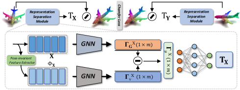
Figure 1: Our UPCR network architecture. Given the source and target point clouds, the graph neural network is applied on the original point coordinates and the distance-based features to encode the global representation and pose-invariant part representation, respectively. Then, the pose-related part representation is produced by the representation separation module. Finally, we use it to regress their respective relative poses w.r.t. the same “latent canonical shape”. And the final rigid transformation is obtained from these two learned poses.

Pose-Related Part Representation. Our core idea is to estimate the rigid motion by learning relative poses w.r.t. a “latent canonical shape” for source and target point clouds from pose-related part representations, which is more reasonable and accurate. To model this pose-related part representation, we propose to “subtract” pose-invariant part from global representation. Then, a natural question is, how to formulate this special subtraction. A straightforward approach is to learn it through neural networks. However, this operation is uninterpretable and difficult to converge. In the following, we design a novel and elegant “representation subtraction”.

Considering that the relative entropy often works as a “distance” between distributions, we formulate our subtraction analogously. Specifically, we first construct the probability distribution of the global representation and the pose-invariant representation, i.e. $\mathbf{q}=\text{softmax}(\Gamma_{\mathbf{G}})$, $\mathbf{p}=\text{softmax}(\Gamma_{\nu})$. Then, we formulate the pose-related part representation as:

$$\Gamma_{\mu}=[\mathbf{p}_{1}\log({\mathbf{p}_{1}}/{\mathbf{q}_{1}}),\mathbf{p}_{2}\log({\mathbf{p}_{2}}/{\mathbf{q}_{2}}),...,\mathbf{p}_{m}\log({\mathbf{p}_{m}}/{\mathbf{q}_{m}})],$$ (5)

where the subscript is the dimension index.

Then, we regress both rotations and translations from the pose-related representations. The Euler angle ${\Omega}\in\mathbb{R}^{3}$ is used to represent the rotation, which is compact and facilitates accurate regression. Afterwards, the relative poses $\mathbf{T}_{\mathbf{X}}$, $\mathbf{T}_{\mathbf{Y}}$ w.r.t. the same “latent canonical shape”, which can be decoded as,

$$\left\{{\begin{aligned} {\Omega}_{\mathbf{X}},\mathbf{t}_{\mathbf{X}}&=h_{\beta}(\Gamma_{\mu}^{\mathbf{X}}),\ \mathbf{R}_{\mathbf{X}}=\mathcal{T}({\Omega}_{\mathbf{X}})\\ {\Omega}_{\mathbf{Y}},\mathbf{t}_{\mathbf{Y}}&=h_{\beta}(\Gamma_{\mu}^{\mathbf{Y}}),\ \mathbf{R}_{\mathbf{Y}}=\mathcal{T}({\Omega}_{\mathbf{Y}})\end{aligned}}\right.,\vspace{-0.2cm}$$ (6)

where $h_{\beta}$ is the MLP parameterized by $\beta$, $\mathcal{T}(\cdot)$ is the function that transforms Euler angle to rotation matrix. We obtain the final rigid transformation as ${\mathbf{R}}=\mathbf{R}_{\mathbf{Y}}{\mathbf{R}_{\mathbf{X}}}^{\mathrm{T}}$, ${\mathbf{t}}=\mathbf{t}_{\mathbf{Y}}-\mathbf{R}{\mathbf{t}_{\mathbf{X}}}$.

II-B Unsupervised Loss

Next, in our representation separation framework, we can transform the source and target point clouds into the canonical coordinate by $\mathbf{T}_{\mathbf{X}}$ and $\mathbf{T}_{\mathbf{Y}}$ respectively, i.e., $\mathbf{X}_{\mathbf{c}}={\mathbf{R}_{\mathbf{X}}}^{\mathrm{T}}(\mathbf{X}-\mathbf{t}_{\mathbf{X}})$, $\mathbf{Y}_{\mathbf{c}}={\mathbf{R}_{\mathbf{Y}}}^{\mathrm{T}}(\mathbf{Y}-\mathbf{t}_{\mathbf{Y}})$. Note that the latent canonical shapes $\mathbf{X}_{\mathbf{c}}$ and $\mathbf{Y}_{\mathbf{c}}$ should be consistent. Here, we use the Chamfer distance to measure the discrepancy between $\mathbf{X}_{\mathbf{c}}$ and $\mathbf{Y}_{\mathbf{c}}$. In this case, any ground truth is not involved. In other words, an unsupervised loss is constructed as,

$$Loss(\mathbf{X}_{\mathbf{c}},\mathbf{Y}_{\mathbf{c}})=\frac{1}{N_{\mathbf{X}}} \sum\limits_{\boldsymbol{x}\in\mathbf{X}_{\mathbf{c}}}\min\limits_{\boldsymbol{y}\in\mathbf{Y}_{\mathbf{c}}}\|\boldsymbol{x}-\boldsymbol{y}\|_{2}^{2}$$ (7)

$$+\frac{1}{N_{\mathbf{Y}}}\sum\limits_{\boldsymbol{y}\in\mathbf{Y}_{\mathbf{c}}}\min\limits_{\boldsymbol{x}\in\mathbf{X}_{\mathbf{c}}}\|\boldsymbol{x}-\boldsymbol{y}\|_{2}^{2}.$$

III Experiments

Implementation Details. We use GNN as the point cloud representation extractor, where $K=24$ of KNN experimentally. The dimension $m=512$. The number of layers $\ell=5$. We train our network for 500 epochs with an initial learning rate of $1e^{-3}$. As our method is unsupervised, we fine-tune the model for 200 epochs with an initial learning rate of $1e^{-4}$ on the test split. We use the Adam optimizer and the experiment is performed in PyTorch 1.0.0 with a batch size of 26.

Dataset and Evaluation Metric. For synthetic dataset ModelNet40 [26], following [23, 24], the rotation and translation along each axis between the source and target are in $[0^{\circ},45^{\circ}]$, $[-0.5,0.5]$. For real dataset 7Scenes [20], following [11], the rotation is initialized in $[0^{\circ},60^{\circ}]$ and the translation is initialized in $[0,1.0]$ along one randomly selected axis. Root mean square error (RMSE) and mean absolute error (MAE) in Euler angle and translation vector, and mean error in $SE(3)$ [3] are used as evaluation metrics, notated as RMSE(R), MAE(R), RMSE(t), MAE(t), and ME(T) respectively.

III-A Evaluation on ModelNet40

Following [23, 24], three experiment settings are applied here: 1) Unseen Point Clouds (UPC): All point clouds are divided into training and test sets with the official setting. 2) Unseen Categories (UC): The first 20 categories in ModelNet40 are used for training and the rest for test. 3) Noisy Data (ND): Random Gaussian noise (i.e. $\mathcal{N}(0,0.01)$, and the sampled noise out of the range of $[-0.05,0.05]$ will be clipped) is added to the UPC setting.

Consistent Point Clouds. Following [23], the input point clouds are consistent here. Two versions of PRNet have been evaluated, i.e., PRNet selects half points as the key points [24] and PRNet* selects all points as the key points. Besides using distance-based feature notated as UPCR w/ Dis, we also test our method using SPFH [17], PFH [18] as pose-invariant feature notated as UPCR w/ SPFH and UPCR w/ PFH respectively. From Table I, for UPC, in all unsupervised methods, UPCR achieves the best performance. Meanwhile, our unsupervised method even obtains better performance under many metrics than supervised methods. Especially, UPCR outperforms the correspondences-free method, PointNetLK by a large margin. For UC, in all unsupervised methods, UPCR significantly outperforms all baselines. Our method achieves higher accuracy under most metrics than those supervised methods. For ND, UPCR is superior to DCP-v2 but inferior to PRNet and PRNet* under RMSE(R) while achieving the best results under other metrics. Then, in all UPCR pipelines, UPCR w/ PFH achieves the most accurate results due to the informative pose-invariant feature.

TABLE I: Evaluation in the consistent point clouds. Note: “✓” indicates the unsupervised method.

Methods		RMSE(R)$\ \downarrow$			MAE(R)$\ \downarrow$			RMSE(t) ($\times 10^{-2}$)$\ \downarrow$			MAE(t) ($\times 10^{-2}$)$\ \downarrow$			ME(T)$\ \downarrow$
		UPC	UC	ND	UPC	UC	ND	UPC	UC	ND	UPC	UC	ND	UPC	UC	ND
PointNetLK[1]		13.751	15.901	15.692	3.893	4.032	3.992	1.990	2.612	2.396	0.445	0.621	0.564	15.217	16.937	16.716
DCP-v2[23]		1.094	3.256	8.417	0.752	2.102	5.685	0.172	0.632	0.117	0.463	2.337	2.337	1.774	4.647	10.140
PRNet[24]		1.722	3.060	3.218	0.665	1.326	1.446	0.637	1.010	0.465	0.759	0.838	0.838	2.579	4.172	5.021
PRNet*[24]		2.090	3.720	3.292	0.894	1.543	1.449	1.098	1.313	1.077	0.815	0.996	0.815	2.765	4.113	4.974
ICP[2]	✓	12.282	12.707	11.971	4.613	5.075	4.497	4.774	4.853	4.832	0.228	0.236	0.234	16.719	16.911	13.276
FGR[30]	✓	20.054	21.323	18.359	7.146	8.077	6.367	4.412	4.578	3.910	1.642	0.181	1.449	24.126	25.037	22.452
ICP+PFH[18]	✓	7.713	10.287	8.751	1.143	2.017	2.376	1.143	1.798	1.004	0.115	0.107	0.193	8.872	12.035	11.284
ICP+SPFH[17]	✓	8.039	10.977	9.082	1.437	2.391	2.753	1.797	1.848	2.034	0.202	0.194	0.223	9.986	14.425	14.028
UPCR w/ Dis	✓	2.774	3.212	5.420	0.623	1.053	1.432	0.023	0.201	0.151	0.005	0.061	0.105	3.524	3.986	6.107
UPCR w/ SPFH	✓	2.563	3.091	4.975	0.584	0.921	1.224	0.020	0.188	0.134	0.004	0.052	0.100	3.233	3.569	5.547
UPCR w/ PFH	✓	2.373	3.011	4.624	0.514	0.823	1.043	0.018	0.156	0.112	0.004	0.040	0.087	3.011	3.164	4.927

Partial-to-Partial. Our method is robust to outliers because the disturbance in the pose-invariant part has been filtered out. Following the common protocol of PRNet [24], we simulate partial scans of $\mathbf{X}$ and $\mathbf{Y}$ by randomly placing a point in 3D space and selecting its 768 nearest neighbors from the consistent point clouds respectively, where there are 1024 points in each original consistent point cloud. The performance is reported in Table II. For UPC, our UPCR achieves the best performance in all unsupervised methods. Besides, we obtain comparable or better results compared with the state-of-the-art PRNet. For UC, UPCR achieves the best performance under all metrics, even outperforms PRNet. For ND, our method achieves the best performance under most evaluation metrics over all unsupervised and supervised methods. These results verify the robustness of our method to partial-to-partial cases. Besides, UPCR w/ PFH achieves the best performance among all UPCR pipelines because PFH feature is more informative.

TABLE II: Evaluation in the partial-to-partial setting.

Methods		RMSE(R)$\ \downarrow$			MAE(R)$\ \downarrow$			RMSE(t)$\ \downarrow$			MAE(t)$\ \downarrow$			ME(T)$\ \downarrow$
		UPC	UC	ND	UPC	UC	ND	UPC	UC	ND	UPC	UC	ND	UPC	UC	ND
PointNetLK[1]		16.735	22.943	19.939	7.550	9.655	9.076	0.045	0.061	0.057	0.025	0.033	0.032	18.264	23.417	21.547
DCP-v2[23]		6.709	9.769	6.883	4.448	6.954	4.534	0.027	0.034	0.028	0.020	0.025	0.021	7.847	10.527	7.912
PRNet[24]		3.199	4.986	4.323	1.454	2.329	2.051	0.016	0.021	0.017	0.010	0.015	0.012	4.428	5.746	5.013
ICP[2]	✓	33.683	34.894	35.067	25.045	25.455	25.564	0.293	0.293	0.294	0.250	0.251	0.250	36.745	38.294	40.012
FGR[30]	✓	11.238	9.932	27.635	2.832	1.952	13.794	0.030	0.038	0.070	0.008	0.007	0.039	13.243	12.476	30.127
ICP+PFH[18]	✓	14.389	10.743	27.976	3.578	4.217	14.278	0.147	0.172	0.144	0.108	0.117	0.193	17.013	12.896	30.104
ICP+SPFH[17]	✓	18.647	24.312	29.904	4.015	4.993	15.673	0.190	0.201	0.159	0.207	0.198	0.214	20.778	27.746	32.368
UPCR w/ Dis	✓	3.901	3.713	5.522	1.518	1.138	1.702	0.009	0.008	0.020	0.004	0.002	0.010	4.542	4.879	6.748
UPCR w/ SPFH	✓	3.728	3.387	5.217	1.274	1.008	1.468	0.008	0.008	0.016	0.004	0.002	0.008	4.034	4.374	6.038
UPCR w/ PFH	✓	3.271	3.014	4.876	1.012	0.971	1.195	0.008	0.007	0.011	0.003	0.002	0.008	3.512	4.014	5.429

III-B Evaluation on 7Scenes

In Table V, we evaluate our UPCR on 7Scenes [20], which is a remote scene RGB-D data including Heads, Office, Chess, Fire, Pumpkin, Redkitchen, Stairs scenes. We use the 3D point cloud information only. Since the real scene data is very challenging, state-of-the-art supervised point cloud registration methods, such as DCP-v2 and PRNet fail to estimate the transformation. For UPCR, we provide the model trained on ModelNet40, fine-tuned on Heads, fine-tuned on the corresponding test scene respectively. Results are consistent: 1) The model trained on ModelNet40 shows poor performance on scene data but is still better than baselines. 2) Models fine-tuned on Heads and corresponding test scenes show accurate and very similar performance, i.e. the model fine-tuned on one scene can obtain accurate results on other scenes.

III-C Ablation Study

1. Rotation Solver. There are several rotation representations, including rotation matrix, 6D expression [31], quaternion, Euler angle, etc., which are compared in Table III. The Euler angle representation achieves the best performance. We reckon this is because the network can converge more easily to achieve better results in a more compact representation.

TABLE III: Performance of UPCR w/ Dis method in different rotation representation solvers on consistent point clouds under UPC.

Methods	Variables	RMSE(R)	MAE(R)	RMSE(t)($\times 10^{-2}$)	MAE(t)($\times 10^{-2}$)	ME(T)
Rotation Matrix	9	34.894	25.455	0.293	0.025	37.976
6D expression	6	7.972	3.810	0.076	0.036	10.286
Quaternion	4	3.502	0.524	0.038	0.005	4.743
Euler Angle	3	2.774	0.623	0.023	0.005	3.524

2. Performance vs. Outliers Ratios. Fig. 2 shows the performance degeneration as outliers ratio increases. Compared to PRNet, our unsupervised UPCR w/ Dis method has comparable rotation estimation and better translation estimation results. Totally speaking, when outliers ratio increases, our method is more robust than these supervised methods.

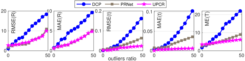
Figure 2: Performance decreases as the outliers ratio (%) increases.

3. Completeness of Pose-Invariant Feature. We can observe that UPCR with more informative pose-invariant features, e.g. SPFH, PFH achieves better performance than using distance-based feature since SPFH and PFH represent the pose-invariant part more completely. Here, to verified this conclusion further, we employ seven pose-invariant features, i.e. distance-based feature, PPF [5], SPFH [17], PFH [18], distance-based + PPF, distance-based + SPFH and distance-based + PPF + SPFH to extract the pose-invariant representation variants, respectively. Then, the global representation, and the seven pose-related representations returned by “subtracting” these variants are used to perform an ablation experiment.

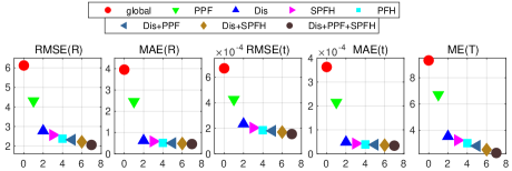
Figure 3: Incremental experiment of pose-invariant feature.

From Fig. 3, regressing pose via the entire point cloud underperforms purified pose-related part representation. The performance of using distance-based + PPF + SPFH is better than using one or two of them. Based on these observations, we conclude that our distance-based feature cannot represent the pose-invariant part completely, and some pose-invariant information still exists in pose-related representation obtained via designed entropy subtraction. Moreover, more informative pose-invariant feature, which results in more purified pose-related representation, helps obtain better registration performance. Although our distance-based feature underperforms several typical features, it has achieved comparable or better performance than the state-of-the-art supervised methods.

4. Time Complexity. We report the average inference time of each input sample with 1024 points on GTX 1080 Ti in Table IV. Our UPCR w/ Dis achieves advanced time-efficiency due to the simple distance-based feature. UPCR w/ PFH shows poor time-efficiency due to the complex feature extraction.

TABLE IV: Inference time on point cloud with 1024 points.

Methods	PointNetLK	DCP	PRNet	PRNet*	UPCR w/ Dis	UPCR w/ SPFH	UCPR w/ PFH
Time(ms)	66.32	10.98	45.48	47.22	9.71	2140.53	8134.34

TABLE V: Evaluation on 7Scenes. ModelNet40 indicates that the model is trained on ModelNet40, Heads means that the model is fine-tuned on Heads, test scene means that the model is fine-tuned on the corresponding test scene.

Methods	Heads			Office			Chess			Fire			Pumpkin			Redkitchen			Stairs
	RMSE(R)	MAE(R)	ME(T)	RMSE(R)	MAE(R)	ME(T)	RMSE(R)	MAE(R)	ME(T)	RMSE(R)	MAE(R)	ME(T)	RMSE(R)	MAE(R)	ME(T)	RMSE(R)	MAE(R)	ME(T)	RMSE(R)	MAE(R)	ME(T)
DCP-v2[23]	79.448	53.914	87.646	77.268	49.594	85.476	71.298	52.921	80.374	75.264	50.924	83.714	70.853	44.758	77.983	79.023	51.043	86.142	75.849	53.269	84.347
PRNet[24]	75.719	49.808	84.276	72.164	48.623	78.146	65.972	47.026	71.419	70.215	43.267	77.842	66.473	42.125	73.982	74.285	45.681	80.276	70.364	47.231	77.451
UPCR w/ Dis(ModelNet40)	23.614	17.823	25.946	18.503	14.308	21.047	20.693	16.232	22.384	19.735	15.467	22.046	20.266	15.738	23.451	19.651	15.254	21.137	22.195	17.477	24.156
UPCR w/ Dis(Heads)	1.424	0.913	2.184	0.997	0.689	1.478	2.576	1.678	3.947	1.093	0.682	2.024	1.161	0.818	2.454	0.967	0.641	1.989	1.291	0.866	3.014
UPCR w/ Dis(test scene)	1.422	0.910	2.220	0.998	0.690	1.466	2.577	1.679	3.920	1.093	0.681	2.019	1.164	0.834	2.462	0.953	0.653	2.011	1.227	0.894	2.917
1-22[2.2pt/1.2pt] UPCR w/ SPFH(ModelNet40)	20.141	15.436	23.778	17.498	13.411	19.766	18.455	14.112	19.978	16.433	13.477	18.479	18.472	14.010	20.147	17.496	14.788	19.022	18.452	15.787	20.196
UPCR w/ SPFH(Heads)	1.221	0.900	2.102	0.879	0.654	1.244	2.334	1.433	3.748	1.007	0.641	1.997	1.024	0.776	2.101	0.756	0.502	1.701	1.204	0.745	2.456
UPCR w/ SPFH(test scene)	1.207	0.801	2.003	0.842	0.614	1.213	2.374	1.441	3.696	1.004	0.593	1.867	0.944	0.798	2.114	0.806	0.602	1.879	1.007	0.787	2.532
1-22[2.2pt/1.2pt] UPCR w/ PFH(ModelNet40)	19.011	14.217	20.179	17.244	13.207	19.463	18.017	13.877	19.062	16.014	13.038	17.844	18.027	13.545	19.233	16.314	14.022	18.131	17.032	13.977	17.936
UPCR w/ PFH(Heads)	1.200	0.900	2.004	0.843	0.642	1.204	2.301	1.377	3.644	1.007	0.601	1.827	1.001	0.731	1.927	0.711	0.422	1.535	1.007	0.745	2.421
UPCR w/ PFH(test scene)	1.113	0.724	1.775	0.802	0.543	1.007	2.075	1.214	3.499	1.004	0.544	1.752	0.902	0.756	2.021	0.788	0.566	1.789	1.001	0.746	2.455
	RMSE(t)	MAE(t)	ME(T)	RMSE(t)	MAE(t)	ME(T)	RMSE(t)	MAE(t)	ME(T)	RMSE(t)	MAE(t)	ME(T)	RMSE(t)	MAE(t)	ME(T)	RMSE(t)	MAE(t)	ME(T)	RMSE(t)	MAE(t)	ME(T)
DCP-v2[23]	0.185	0.123	-	0.176	0.105	-	0.192	0.116	-	0.201	0.114	-	0.193	0.113	-	0.179	0.122	-	0.202	0.137	-
PRNet[24]	0.080	0.054	-	0.077	0.062	-	0.093	0.071	-	0.088	0.063	-	0.079	0.068	-	0.083	0.065	-	0.079	0.059	-
UPCR w/ Dis(ModelNet40)	0.044	0.031	-	0.048	0.032	-	0.051	0.038	-	0.047	0.035	-	0.061	0.045	-	0.048	0.036	-	0.054	0.041	-
UPCR w/ Dis(Heads)	0.026	0.018	-	0.023	0.018	-	0.030	0.021	-	0.019	0.014	-	0.029	0.019	-	0.020	0.014	-	0.023	0.015	-
UPCR w/ Dis(test scene)	0.025	0.020	-	0.021	0.015	-	0.033	0.027	-	0.022	0.017	-	0.024	0.021	-	0.022	0.013	-	0.021	0.012	-
1-22[2.2pt/1.2pt] UPCR w/ SPFH(ModelNet40)	0.032	0.027	-	0.040	0.026	-	0.041	0.032	-	0.042	0.030	-	0.055	0.041	-	0.042	0.032	-	0.047	0.036	-
UPCR w/ SPFH(Heads)	0.023	0.016	-	0.021	0.017	-	0.027	0.018	-	0.017	0.011	-	0.021	0.015	-	0.017	0.011	-	0.019	0.012	-
UPCR w/ SPFH(test scene)	0.023	0.017	-	0.020	0.015	-	0.030	0.025	-	0.019	0.015	-	0.020	0.020	-	0.020	0.011	-	0.018	0.010	-
1-22[2.2pt/1.2pt] UPCR w/ PFH(ModelNet40)	0.030	0.024	-	0.035	0.025	-	0.037	0.030	-	0.034	0.030	-	0.050	0.040	-	0.042	0.030	-	0.043	0.034	-
UPCR w/ PFH(Heads)	0.023	0.015	-	0.020	0.017	-	0.025	0.018	-	0.016	0.010	-	0.020	0.015	-	0.016	0.010	-	0.019	0.011	-
UPCR w/ PFH(test scene)	0.022	0.016	-	0.018	0.015	-	0.027	0.022	-	0.017	0.015	-	0.018	0.017	-	0.019	0.010	-	0.018	0.010	-

IV Conclusion

In this paper, we have proposed a correspondence-free unsupervised 3D point cloud registration method from the representation separation perspective. Our proposed method not only filters out the disturbance in pose-invariant representation but also is robust to partial-to-partial or noisy point clouds. Experiments on benchmark datasets demonstrate the superiority and robustness of our unsupervised 3D point cloud registration method, which achieves comparable if not better performance than the state-of-the-art supervised methods.

References

- [1] Y. Aoki, H. Goforth, R. A. Srivatsan, and S. Lucey, “Pointnetlk: Robust & efficient point cloud registration using pointnet,” in Proceedings of the IEEE Conference on Computer Vision and Pattern Recognition, 2019, pp. 7163–7172.
- [2] P. J. Besl and N. D. McKay, “A method for registration of 3-d shapes,” IEEE Transactions on Pattern Analysis & Machine Intelligence, vol. 14, no. 2, pp. 239–256, 1992.
- [3] R. Brégier, F. Devernay, L. Leyrit, and J. L. Crowley, “Defining the pose of any 3d rigid object and an associated distance,” International Journal of Computer Vision, vol. 126, no. 6, pp. 571–596, 2018.
- [4] H. Cao, R. Zhan, Y. Ma, C. Ma, and J. Zhang, “Lfnet: Local rotation invariant coordinate frame for robust point cloud analysis,” IEEE Signal Processing Letters, vol. 28, pp. 209–213, 2021.
- [5] H. Deng, T. Birdal, and S. Ilic, “Ppf-foldnet: Unsupervised learning of rotation invariant 3d local descriptors,” in Proceedings of the European Conference on Computer Vision, 2018, pp. 620–638.
- [6] H. Deng, T. Birdal, and S. Ilic, “3d local features for direct pairwise registration,” in Proceedings of the IEEE Conference on Computer Vision and Pattern Recognition, 2019, pp. 3244–3253.
- [7] S. Deng and Q. Dong, “Ga-net: Global attention network for point cloud semantic segmentation,” IEEE Signal Processing Letters, vol. 28, pp. 1300–1304, 2021.
- [8] L. Ding and C. Feng, “Deepmapping: Unsupervised map estimation from multiple point clouds,” in Proceedings of the IEEE Conference on Computer Vision and Pattern Recognition, 2019, pp. 8650–8659.
- [9] Z. Gojcic, C. Zhou, J. D. Wegner, and A. Wieser, “The perfect match: 3d point cloud matching with smoothed densities,” in Proceedings of the IEEE Conference on Computer Vision and Pattern Recognition, 2019, pp. 5545–5554.
- [10] R. Huang, D. Hong, Y. Xu, W. Yao, and U. Stilla, “Multi-scale local context embedding for lidar point cloud classification,” IEEE Geosci. Remote. Sens. Lett., vol. 17, no. 4, pp. 721–725, 2020.
- [11] X. Huang, G. Mei, and J. Zhang, “Feature-metric registration: A fast semi-supervised approach for robust point cloud registration without correspondences,” in Proceedings of the IEEE Conference on Computer Vision and Pattern Recognition, 2020, pp. 11 363–11 371.
- [12] B. D. Lucas and T. Kanade, “An iterative image registration technique with an application to stereo vision,” in Proceedings of the International Joint Conference on Artificial Intelligence, 1981, pp. 674–679.
- [13] H. Luo, Q. Zheng, C. Wang, and W. Guo, “Boundary-aware and semiautomatic segmentation of 3-d object in point clouds,” IEEE Geosci. Remote. Sens. Lett., vol. 18, no. 5, pp. 910–914, 2021.
- [14] G. D. Pais, S. Ramalingam, V. M. Govindu, J. C. Nascimento, R. Chellappa, and P. Miraldo, “3dregnet: A deep neural network for 3d point registration,” in Proceedings of the IEEE Conference on Computer Vision and Pattern Recognition, 2020, pp. 7191–7201.
- [15] C. R. Qi, H. Su, K. Mo, and L. J. Guibas, “Pointnet: Deep learning on point sets for 3d classification and segmentation,” in Proceedings of the IEEE Conference on Computer Vision and Pattern Recognition, 2017, pp. 652–660.
- [16] C. R. Qi, L. Yi, H. Su, and L. J. Guibas, “Pointnet++: Deep hierarchical feature learning on point sets in a metric space,” in Proceedings of the Advances in Neural Information Processing Systems, 2017, pp. 5099–5108.
- [17] R. B. Rusu, N. Blodow, and M. Beetz, “Fast point feature histograms (fpfh) for 3d registration,” in Proceedings of the IEEE International Conference on Robotics and Automation, 2009, pp. 3212–3217.
- [18] R. B. Rusu, N. Blodow, Z. C. Marton, and M. Beetz, “Aligning point cloud views using persistent feature histograms,” in Proceedings of the International Conference on Intelligent Robots and Systems. IEEE, 2008, pp. 3384–3391.
- [19] V. Sarode, X. Li, H. Goforth, Y. Aoki, A. Dhagat, R. A. Srivatsan, S. Lucey, and H. Choset, “One framework to register them all: Pointnet encoding for point cloud alignment,” arXiv:1912.05766, 2019.
- [20] J. Shotton, B. Glocker, C. Zach, S. Izadi, A. Criminisi, and A. W. Fitzgibbon, “Scene coordinate regression forests for camera relocalization in rgb-d images,” in Proceedings of the IEEE Conference on Computer Vision and Pattern Recognition, 2013, pp. 2930–2937.
- [21] W. Sun, A. Tagliasacchi, B. Deng, S. Sabour, S. Yazdani, G. Hinton, and K. M. Yi, “Canonical capsules: Unsupervised capsules in canonical pose,” arXiv:2012.04718, 2020.
- [22] G. Wan, X. Yang, R. Cai, H. Li, Y. Zhou, H. Wang, and S. Song, “Robust and precise vehicle localization based on multi-sensor fusion in diverse city scenes,” in Proceedings of the IEEE International Conference on Robotics and Automation, 2018, pp. 4670–4677.
- [23] Y. Wang and J. M. Solomon, “Deep closest point: Learning representations for point cloud registration,” in Proceedings of the IEEE International Conference on Computer Vision, 2019, pp. 3523–3532.
- [24] Y. Wang and J. M. Solomon, “Prnet: Self-supervised learning for partial-to-partial registration,” in Proceedings of the Advances in Neural Information Processing Systems, 2019, pp. 8814–8826.
- [25] Y. Wang, Y. Sun, Z. Liu, S. E. Sarma, M. M. Bronstein, and J. M. Solomon, “Dynamic graph cnn for learning on point clouds,” ACM Transactions on Graphics, vol. 38, no. 5, pp. 1–12, 2019.
- [26] Z. Wu, S. Song, A. Khosla, F. Yu, L. Zhang, X. Tang, and J. Xiao, “3d shapenets: A deep representation for volumetric shapes,” in Proceedings of the IEEE Conference on Computer Vision and Pattern Recognition, 2015, pp. 1912–1920.
- [27] W. Y. Yan, A. Shaker, and N. El-Ashmawy, “Urban land cover classification using airborne lidar data: A review,” Remote Sens. Environ., vol. 158, pp. 295–310, 2015.
- [28] W. Yuan, B. Eckart, K. Kim, V. Jampani, D. Fox, and J. Kautz, “Deepgmr: Learning latent gaussian mixture models for registration,” in Proceedings of the European Conference on Computer Vision, 2020, pp. 733–750.
- [29] C. Zhao, H. Guo, J. Lu, D. Yu, D. Li, and X. Chen, “ALS point cloud classification with small training data set based on transfer learning,” IEEE Geosci. Remote. Sens. Lett., vol. 17, no. 8, pp. 1406–1410, 2020.
- [30] Q.-Y. Zhou, J. Park, and V. Koltun, “Fast global registration,” in Proceedings of the European Conference on Computer Vision, 2016, pp. 766–782.
- [31] Y. Zhou, C. Barnes, J. Lu, J. Yang, and H. Li, “On the continuity of rotation representations in neural networks,” in Proceedings of the IEEE Conference on Computer Vision and Pattern Recognition, 2019, pp. 5745–5753.