Stability analysis of hybrid systems with higher order transverse discontinuity mapping

Abstract

This article generalizes the implementation of higher order corrections to state transition matrices during instantaneous reversals in hybrid dynamical systems impacting a discontinuity boundary transversally. A closed form expression for saltation terms in systems possessing a degree of smoothness zero is derived. The difference in flight times of two closely initiated trajectories in state space to the impacting surface has been estimated up to $\mathcal{O}(2)$. A comparison of the times of impact estimated with the first order approximation reveals that higher order corrections lead to a significant improvement of estimates. Next, two new algorithms to estimate the Lyapunov spectrum and Floquet multipliers for piecewise-smooth systems have been presented using the derived second order corrections. Stability analyses are subsequently carried out using the proposed framework for two representative cases i.e., of a hard impact oscillator and a pair impact oscillator. It is established that the obtained Floquet multipliers and Lyapunov spectrum accurately predict the stability of the dynamical states, as validated by their corresponding bifurcation diagrams.

1 Introduction

Floquet analysis for the study of piece-wise smooth dynamical systems requires introduction of state transitions at impacting conditions nayfeh2008applied . This is done with the help of linearized saltation matrices. These matrices can be obtained by retaining only the first order terms of the Taylor expansion of the state at the instant of impact. Such an analysis is helpful in the quantisation of stability in the infinitesimally close local neighborhood quite well. However, if the observation is to be made in a wider region in the local neighbourhood or if the periodicity of the steady state is respectively high, then the errors in the prediction of the resetting state post interaction with the discontinuity boundary by only retaining the first order terms could be largely erroneous. As the intensity of this perturbation grows, the errors in the prediction of the perturbed saltating trajectory while only the first order terms are retained could be significant, rendering the analysis inadequate. This could also consequently lead to incorrect predictions of the stability state. This is the problem this work attempts to resolve with a generalized framework containing higher order terms. A formal description of the above mentioned terms alongwith some contextual remarks have been provided below.

Piecewise-smooth (PWS) systems refer to continuous or discrete time dynamical systems where the state space is compartmentalised into subspaces by instantaneous changes in dynamics. These abrupt transitions occur in time scales much lesser than the time scales of the dynamics of the system and are thus represented by discontinuous boundaries. A sub-class of such systems is hybrid dynamical systems, where the transitions at the barriers are governed by re-initialization rules of state van2000introduction . The dynamics of the vector field within each subspace obeys different functional formsbernardo2008piecewise . Such systems often show rich phenomenological behaviour which is not typical of smooth dynamical systems di2010discontinuity ; chin1994grazing ; jiang2017grazing ; pavlovskaia2004two ; simpson2020nordmark . These behaviours include the occurrence of discontinuity induced bifurcations (DIBs), that occur due to the interaction of the trajectories with the boundary. This phenomenon is known as a border collision and leads to occurrences like grazing, sticking, sliding and period adding cascades piiroinen2004chaos ; oestreich1996bifurcation ; oestreich1997analytical ; popp1999numerical ; shaw1983periodically ; fredriksson2000normal ; rounak2020bifurcations . Parametric investigations of DIBs have revealed an unconventional route to chaos i.e., via grazing.

Stability analyses of such PWS systems yield insights into the implications of occurrence of border collisions on the system dynamics. Measures like Lyapunov exponents (LE) oseledec1968multiplicative ; pesin1977characteristic ; benettin1980lyapunov1 ; bennetin1980lyapunov2 , measures of entropy benettin1976kolmogorov ; termonia1984kolmogorov and Floquet multipliers floquet1883linear ; nayfeh2008applied have been devised to qualitatively predict the asymptotic stability of smooth dynamical systems. However, when the dynamics is piecewise-smooth, these stability analyses need to account for the switch in dynamics at instants of border collisions. Then the fundamental solution matrix describing the attractor comprises of multiplication of exponential matrices corresponding to the evolution through the smooth part of the subsystems and saltation matrices corresponding to the transitions through switching conditions, multiplied in the sequence of their occurrence. This was addressed by Coleman et al. coleman1997motions and later taken up by Leine et al. in his work on obtaining the invariants of the fundamental solution matrix (FSM) for the Hill’s equation leine2012non . Serveta et al. studied the stability of impact oscillators by implementing contact models between the oscillator and a movable barrier interacting with it. Similar methods, especially applicable for stability analysis of PWS hybrid systems, exist in the literature lamba1994scaling ; mandal2013automated .

Numerical methods to acquire the LE spectrum by evaluating Jacobians from the functional form of the governing equations or by reconstruction of state space from time histories do exist for smooth systems rosenstein1993practical ; wolf1985determining . However, this is not straightforward for a nonsmooth system as the Jacobian matrix of such systems is ill conditioned, resulting in large and unacceptable errors in the computational estimation of LEs. De Souza et al. de2004calculation proposed an algorithm to compute the LE spectrum for impacting systems by analytically reducing the state equations to a transcendental map. In this formulation, the eigenvalues of this map represent the LE spectrum. Jin et al. jin2006method obtained the LE spectrum for an impacting system by studying the dynamics on a suitable Poincaré section, where the Jacobian matrix near border collision was evaluated. The work by Stefanski stefanski2000estimation proposed computing the state difference vector between the dynamics of a pair of coupled PWS systems and deduced its synchronization state to compute the largest Lyapunov exponent. Following this work, Stefanski stefanski2003estimation proposed a perturbative approach to estimate the dominant LE of two closely spaced PWS system when one of the systems is perturbed. This method is suitable for systems that possess discontinuities as well as time delays. Recently, Stefanski stefanski2005evaluation presented a method wherein the LE spectrum is computed for nonsmooth systems by circumventing discontinuities. This has been done by considering the value of the function at the previous time-step and continuing integration of the perturbed trajectory until it encounters a discontinuity. Balcerzak et al. balcerzak2020determining presented a method to compute LEs applicable to continuous-time dynamical systems as well as discrete maps by estimating the Jacobi matrix at the instant of border collision. A method based on the scalar product of a system’s perturbation and its derivative also exists dabrowski2012estimation . Müller (muller1995calculation ) proposed an algorithm to evaluate the LE spectrum for a generalised dynamical system with discontinuities using a linearized approximation of the transitions at the instant of discontinuities. Li et al. li2018chaotic presented a method to analytically derive the LE of a nonsmooth dynamical system by evaluating the transfer matrix before, after and during the instant of a border collision at a discontinuous boundary.

Looking at the existing literature, it appears that the investigations of PWS systems fundamentally rely on the linearization of the system at the instants of border collision. This necessitates the investigation of dynamics at border collision with higher order corrections. Yin et al. yin2018higher studied bifurcations of an impact oscillator at near-grazing dynamics using higher order zero-time discontinuity mapping (ZDM). The trajectories that undergo transverse interactions, modeled via transverse discontinuity mapping (TDM), however, is a more generalized case, which has not been studied. Here, the trajectories undergo border collision with non-zero velocities. In such a case, two closely spaced trajectories might exponentially diverge on interaction with a barrier budd1995effect . At some parameter value, the time difference between two consecutive border collision might be large, as a consequence of which the separation between two closely spaced trajectories will grow in time. This effect becomes more pronounced when the underlying dynamics for the chosen parameter is chaotic. The assumption of linearization in the neighbourhood of an impact might fail, especially when the separation becomes larger than the radius of convergence of the respective linearizationacary2009higher . Moreover, there exists a time difference between the instant of border collision for two perturbed trajectories in the state space. However, TDM defined by the saltation matrix at the instant of border collision relies on a linearized derivation of this time difference bernardo2008piecewise .

This paper derives this time difference between perturbed trajectories at the instant of border collision with higher order corrections. The proposed corrections to the time difference accounts for the functional form of the driving force for a PWS system executing border collision transversally. This implementation offers significant improvement over the results obtained using the corresponding linearization theory. TDM governed by a linearized saltation matrix defines a map or a reset condition for trajectories executing transverse border collisions. Typically PWS systems undergo several border collisions before attaining a steady state. Therefore, errors in the linearized TDM will accumulate every time a mapping occurs, ultimately leading to an incorrect prediction of the steady state. A TDM of the perturbed trajectory with higher order terms when a hybrid system undergoes a border collision is thus proposed. This method is implemented to accurately map the trajectories of a hybrid system to the same subspace at the instant of border collision. The growth or decay in evolution of disturbances in initially perturbed trajectories is quantified using the LE spectra. The proposed methodology to evaluate the LE spectra does not require any prior knowledge of the analytical solution at the instant of border collision as seen in the case for transcendental maps. Subsequent to the proposed TDM for a generalized PWS system, algorithms to compute saltation matrix with higher order corrections are proposed. To demonstrate the efficacy of the method, Floquet analysis has been carried out. The obtained results are compared with the corresponding bifurcation diagram for verification. The algorithms presented in this paper can be used as a benchmark tool to study the long time dynamics of the steady state for an arbitrary PWS systems where the exact analytical solution near the discontinuity boundary is not known. This work can be generalized to hybrid dynamical systems with higher dimensions, multiple barriers exhibiting exceedingly complex dynamics. The strength of this approach has been demonstrated with the use of representative examples of the simplest hybrid dynamical systems.

This article is structured as follows. In Sec. 2 a discrete mapping of state transitions at the instant of border collision for a hybrid system is derived. This mapping takes into account the second order terms in expansions. Section 3 introduces two hybrid oscillators with 1 and 2 discontinuity boundaries respectively and presents their stability analysis. A comparison of the results obtained from $\mathcal{O}(1)$ and $\mathcal{O}(2)$ approximations is discussed. Section 4 extends the implementation of the derived TDM shown in Sec. 2 to numerically obtain the Lyapunov spectrum. Section 5 describes the algorithm to evaluate saltation matrices using the proposed TDM, followed by an eigenvalue analysis of the obtained monodromy matrix. The stability of the aforementioned dynamical systems is analysed by obtaining the corresponding Floquet multipliers. The results are corroborated with the respective bifurcation diagrams. Section 6 summarises the principal outcomes of this study.

2 Mathematical formulation

The generalized form of a dynamical system represented by states $\vec{x}(t)$, where $\vec{x}\in\mathbb{R}^{n}$, and its corresponding variational form can be written in the state space formulation as Eq. (1)

$$\frac{d\vec{x}}{dt} =\vec{F}(\vec{x}),$$ (1)

$$\frac{d\vec{y}}{dt} =(\vec{\nabla}\vec{F}(\vec{x}))^{T}\cdot\vec{y}$$

where $\vec{y}$ is a perturbation to the system $\vec{x}$. The variational form that governs the dynamics of nearby perturbed trajectories is generally derived with a linearized approximation. However, for PWS systems, different perturbed trajectories reach the discontinuity boundary at different instants of time; see Fig. 1. The difference in the flight times can lead to estimation of erroneous trajectories after an implementation of a linearized TDM at the instant of border collision. This carries significance when the separation between trajectories is greater than the radius of convergence of $\vec{F}(\vec{x})$. To obtain the evolution of perturbed trajectories near border collision, taking higher order terms into consideration is thus necessary.

The evolution of two closely spaced trajectories is depicted in the simplistic case of a 2-dimensional state space; see Fig. 1. Two closely spaced points $\vec{x}_{p}$ and $\vec{\hat{x}}$ are initiated at the Poincaré section $\Sigma_{1}$ where they start evolving from the same instant. $\vec{\hat{x}}$ represents a perturbed trajectory from $\vec{x}_{p}$, i.e. $\vec{\hat{x}}=\vec{x}_{p}+\vec{y}$, where $\vec{y}$ is a infinitesimal perturbation provided to the original system at the beginning of its evolution, denoted by Eq. (1). After evolving in time, at $t=t_{0}$, the orbit $\vec{x}_{p}$ impacts the hard surface, $\Sigma_{2}$ at $\vec{x}_{i}$. At this instant, when the path described by $\vec{x}$ impacts the surface $\Sigma_{2}=\{\vec{x}\in\mathbb{R}^{n}:H(\vec{x})=0\}$ , the trajectory gets mapped to $\vec{R}(\vec{x}_{i})$. Here, $\vec{R}(\vec{x})$ represents a restitutive law governing the state of the trajectory at impact whereas $H(\vec{x})=0$ models the impacting condition. The reset map $\vec{R}$ is a typical example of a nonsmooth event that arises in systems exhibiting switchings. Applying the map $\vec{R}(\vec{x}_{0})$ to the perturbed trajectory $\vec{\hat{x}}(t_{0})=\vec{x}_{0}$ at the instant of impact $t_{0}$ will result in an incorrect prediction of state, as it does not lie on the impacting surface $\Sigma_{2}$ at that instant. Thus the difference in the flight times of the two paths $\vec{x}_{i}$ and $\vec{x}_{0}$ is to be taken into account. The corresponding expression for the flight time is described below. In case of absence of the barrier, if the perturbed trajectory was initiated at $\vec{x}_{4}$, it would take the same flight time to arrive at $\Sigma_{2}$ as the perturbed trajectory at $\vec{x}_{0}$ would take to reach $\Sigma_{2}$ at $\vec{x}_{2}$. The mapping of the perturbed path $\vec{x}_{0}$ to $\vec{x}_{4}$ at the instant of border collision of the actual trajectory is shown in Fig. 1. This discrete mapping accounts for the state transition at impact and is expressed in terms of a saltation matrix in the linearized form. The corresponding equation governing the saltation matrix incorporating higher order terms is presented next.

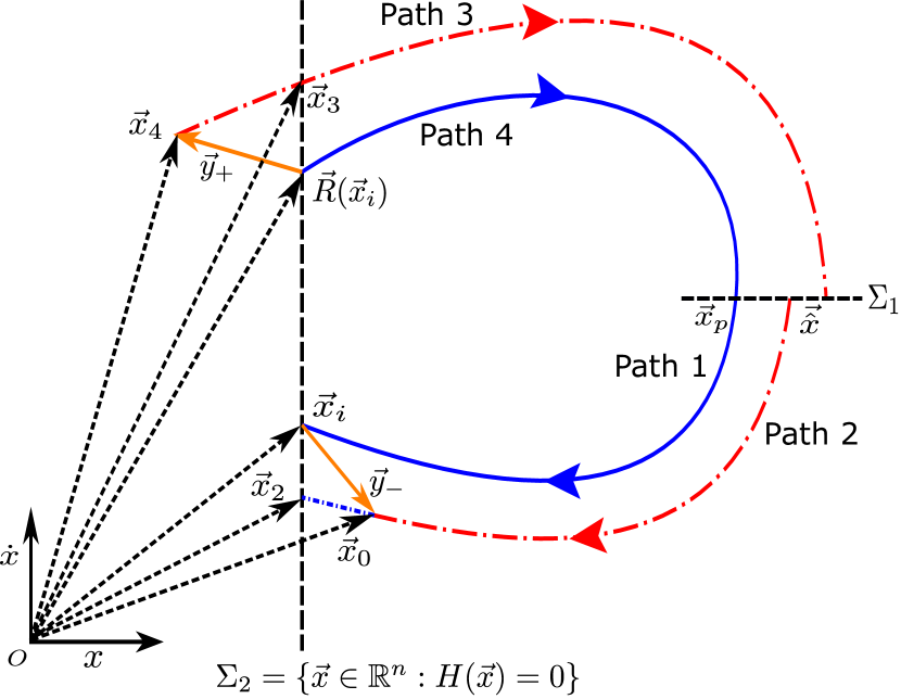
Figure 1: A schematic of the phase portrait of two nearby trajectories exhibiting border collision at $\Sigma_{2}$. The blue line shows the actual trajectory. The red dashed line denotes the perturbed trajectory. The black dashed line $\Sigma_{1}$ denotes the Poincaré section from which both the trajectories are initiated and $\Sigma_{2}$ denotes the discontinuity boundary. The amber line denotes the perturbation vector.

If $t_{0}$ represents the instant of impact of the actual trajectory, a Taylor expansion of $\vec{x}(t)$ about $t=t_{0}$ and $\vec{F}(\vec{x})$ about $\vec{x}=\vec{x}_{0}$ up to $\mathcal{O}(2)$ gives

$$\vec{x}(t)=\vec{x}(t_{0}) +\Delta t\ \vec{F}(\vec{x}_{0})$$ (2)

$$\quad+\frac{1}{2}\Delta t^{2}\ \vec{\nabla}\vec{F}(\vec{x}(t_{0}))^{T}\cdot\vec{F}(\vec{x}(t_{0}))$$

$$\qquad+\mathcal{O}(3)$$

$$\vec{F}(\vec{x})=\vec{F}(\vec{x}_{0}) +\vec{\nabla}\vec{F}(\vec{x}_{0})^{T}\cdot\vec{\Delta x}$$ (3)

$$\quad+\frac{1}{2}\begin{bmatrix}\vec{\Delta x}^{T}\cdot H_{1}\cdot\vec{\Delta x}\\ \vec{\Delta x}^{T}\cdot H_{2}\cdot\vec{\Delta x}\\ \end{bmatrix}$$

$$\qquad+\mathcal{O}(3)$$

Here, $H_{i}$s denote the Hessian matrices of each component $f_{i}(\vec{x})$ of $\vec{F}(\vec{x})$ i.e., $H_{i}$ defined as the Jacobian of $\vec{\nabla}f_{i}(\vec{x})$ or $\vec{\nabla}(\vec{\nabla}f_{i}(\vec{x}))^{T}$. Let $\delta$ be the time taken for the perturbed trajectory $\vec{\hat{x}}$ to reach impact surface $\Sigma_{2}$ from $\vec{x}(t_{0})=\vec{x}_{0}$ to $\vec{x}(t_{0}+\delta)=\vec{x}_{2}$. Therefore, $\vec{x}_{2}$ is approximated by taking a Taylor expansion of $\vec{\hat{x}}$ along path 2 about $t=t_{0}$ (i.e., $\vec{x}(t_{0})=\vec{x}_{0})$ evaluated at $t=t_{0}+\delta$ up to $\mathcal{O}(2)$ giving

$$\vec{x}_{2}=\vec{x}_{0}+\delta\ \vec{F}(\vec{x}_{0}) +\frac{1}{2}\delta^{2}\ \vec{\nabla}\vec{F}(\vec{x}_{0})^{T}\cdot\vec{F}(\vec{x}_{0})$$ (4)

$$\quad+\mathcal{O}(3)$$

$\vec{F}(\vec{x}_{0})$ in Eq. (4) is approximated by a Taylor expansion of $\vec{F}(\vec{x})$ along path 1 about $\vec{x}_{i}$ and evaluated at $\vec{x}=\vec{x}_{0}$. Retaining terms up to $\mathcal{O}(2)$, $\vec{x}_{2}$ becomes,

$$\vec{x}_{2}=\vec{x}_{0} +\delta\ [\vec{F}(\vec{x}_{i})+\vec{\nabla}\vec{F}(\vec{x}_{i})^{T}\cdot\vec{y}_{-}]$$

$$+\frac{1}{2}\delta^{2}\ \vec{\nabla}\vec{F}(\vec{x}_{i})^{T}\cdot\vec{F}(\vec{x}_{i})+\mathcal{O}(3)$$ (5)

where $\vec{y}_{-}$ is the perturbed vector at the instant of impact (i.e. $\vec{x}_{0}=\vec{x}_{i}+\vec{y}_{-}$). Then, the equation for the impacting surface $H(\vec{x})$ expanded about the state at impact $\vec{x}_{i}$ up to $\mathcal{O}(2)$ and evaluated at $\vec{x}=\vec{x}_{2}$ is given by

$$H(\vec{x}_{2})=\ H(\vec{x}_{i})+\vec{\nabla}H(\vec{x}_{i})^{T}\cdot(\vec{x}_{2}-\vec{x}_{i})$$ (6)

$$\quad+\frac{1}{2}(\vec{x}_{2}-\vec{x}_{i})^{T}\cdot\vec{\nabla}(\vec{\nabla}H)^{T}\cdot(\vec{x}_{2}-\vec{x}_{i})$$

$$\qquad+\mathcal{O}(3)$$

Using Eq. (2) in Eq. (6) and $H(\vec{x}_{i})=H(\vec{x}_{2})=0$ (since $\vec{x}_{i}$ and $\vec{x}_{2}$ lie on the impacting surface $\Sigma_{2}$), the time difference in border collision between two closely spaced trajectories, i.e. $\delta$ can be solved up to $\mathcal{O}(2)$. The result is a quadratic equation in $\delta$ given by Eq. (7).

$$\delta^{2}\Big{(} \vec{\nabla}H(\vec{x}_{i})^{T}\cdot\vec{\nabla}\vec{F}(\vec{x}_{i})^{T}\cdot\vec{F}(\vec{x})+\vec{F}(\vec{x}_{i})^{T}\cdot\vec{\nabla}(\vec{\nabla}H(\vec{x}_{i}))^{T}\cdot\vec{F}(\vec{x}_{i})\Big{)}+\delta\Big{(}2\vec{\nabla}H(\vec{x}_{i})^{T}\cdot\vec{F}(\vec{x}_{i})$$ (7)

$$+2\vec{\nabla}H(\vec{x}_{i})^{T}\cdot\vec{\nabla}\vec{F}(\vec{x}_{i})^{T}\cdot\vec{y}+\vec{y}^{T}\cdot\vec{\nabla}(\vec{\nabla}H(\vec{x}_{i}))^{T}\cdot\vec{F}(\vec{x}_{i})+\vec{F}(\vec{x}_{i})^{T}\cdot\vec{\nabla}(\vec{\nabla}H(\vec{x}_{i}))^{T}\cdot\vec{y}\Big{)}$$

$$\quad+\vec{y}^{T}\cdot\vec{\nabla}(\vec{\nabla}H(\vec{x}_{i}))^{T}\cdot\vec{y}+2\vec{\nabla}H(\vec{x}_{i})^{T}\cdot\vec{y}+\mathcal{O}(3)=0$$

The mapping of $\vec{x}_{0}$ to $\vec{x}_{4}$ at the instant of border collision must satisfy $\vec{x}_{4}(t_{0}+\delta)=\vec{x}_{3}$ where $\vec{x}_{3}=\vec{R}(\vec{x}_{2})$; see Fig. 1. This ensures that any perturbed trajectory initiated at $\vec{\hat{x}}(t)$ is correctly mapped on the impact surface $\Sigma_{2}$ to $\vec{x}_{3}$ at time $t_{0}+\delta$. This is a parallel occurrence to the instance when the system at $\vec{x}_{i}$ impacts $\Sigma_{2}$ at $t=t_{0}$. The functional form of $\vec{x}_{4}$ is approximated by expanding $\vec{x}_{3}$ along path 3 about $t=0$. Thus in the absence of $\Sigma_{2}$, $\vec{x}_{4}$ would naturally evolve to $\vec{x}_{3}$ after time $\delta$. Thus $\vec{x}_{4}$ is obtained by expanding and evaluating $\vec{x}_{3}$ backwards in time $t=-\delta$, i.e.,

$$\vec{x}_{4}=\vec{x}_{3}-\delta\ \vec{F}(\vec{x}_{3}) +\frac{1}{2}\delta^{2}\ \vec{\nabla}\vec{F}(\vec{x}_{3})^{T}\cdot\vec{F}(\vec{x}_{3})$$ (8)

$$\quad+\mathcal{O}(3)$$

where $\vec{x}_{3}=\vec{R}(\vec{x}_{2})$. Expanding $\vec{R}(\vec{x})$ about $\vec{x}_{i}$ gives

$$\vec{R}(\vec{x})=\vec{R}(\vec{x}_{i}) +\vec{\nabla}\vec{R}(\vec{x}_{i})^{T}\cdot\vec{\Delta x}$$ (9)

$$\quad+\frac{1}{2}\begin{bmatrix}\vec{\Delta x}^{T}\cdot\tilde{H}_{1}\cdot\vec{\Delta x}\\ \vec{\Delta x}^{T}\cdot\tilde{H}_{2}\cdot\vec{\Delta x}\\ \end{bmatrix}$$

$$\qquad+\mathcal{O}(3)$$

where $\vec{\Delta x}=\vec{x}-\vec{x}_{i}$ and $\tilde{H}_{i}$ are the Hessian matrices of each component $r_{i}(\vec{x})$ of $\vec{R}(\vec{x})$. These Hessian matrices are defined as the Jacobian of $\vec{\nabla}r_{i}(\vec{x})$ or $\vec{\nabla}(\vec{\nabla}r_{i}(\vec{x}))^{T}$. An approximation of $\vec{R}(\vec{x}_{2})$ using Eq. (2) up to $\mathcal{O}(2)$ results in the following expression; see Eq. (10).

$$\vec{R}(\vec{x}_{2})=\ \vec{R}(\vec{x}_{i})+\vec{\nabla}\vec{R}(\vec{x}_{i})^{T}\cdot\Big{(}\vec{y}_{-}+\delta\vec{F}(\vec{x}_{i})$$ (10)

$$+\delta\vec{\nabla}\vec{F}(\vec{x}_{i})^{T}\cdot\vec{y}_{-}+\frac{1}{2}\delta^{2}\vec{\nabla}\vec{F}(\vec{x}_{i})^{T}\cdot\vec{F}(\vec{x}_{i})\Big{)}$$

$$\quad+\frac{1}{2}\begin{bmatrix}[\vec{y}_{-}+\delta\vec{F}(\vec{x}_{i})]^{T}\cdot\vec{\nabla}(\vec{\nabla}r_{1})^{T}\cdot[\vec{y}_{-}+\delta\vec{F}(\vec{x}_{i})]\\ [\vec{y}_{-}+\delta\vec{F}(\vec{x}_{i})]^{T}\cdot\vec{\nabla}(\vec{\nabla}r_{2})^{T}\cdot[\vec{y}_{-}+\delta\vec{F}(\vec{x}_{i})]\end{bmatrix}$$

$$\qquad+\mathcal{O}(3)$$

where $r_{1}$ and $r_{2}$ are the components of the map $\vec{R}(\vec{x})$. Terms up to $\mathcal{O}(2)$ is taken in $\vec{\Delta x}=\vec{x}_{2}-\vec{x}_{i}$. One can then evaluate $\vec{F}(\vec{x}_{3})$ as mentioned in Eq. (8) as an expansion of $\vec{F}(\vec{x})$ along path 4 about $\vec{R}(\vec{x}_{i})$. Taking terms upto $\mathcal{O}(1)$ in $\vec{F}(\vec{x})$ yields

$$\vec{F}(\vec{x}_{3}) =\vec{F}(\vec{R}(\vec{x}_{i}))$$ (11)

$$\quad+\vec{\nabla}\vec{F}(\vec{R}(\vec{x}_{i}))^{T}\cdot\Big{(}\vec{\nabla}\vec{R}(\vec{x}_{i})^{T}\cdot\vec{y}_{-}$$

$$\qquad+\delta\ \vec{\nabla}\vec{R}(\vec{x}_{i})^{T}\cdot\vec{F}(\vec{x}_{i})\Big{)}+\mathcal{O}(2)$$

Now, substituting the expressions for $\vec{R}(\vec{x}_{2})$, $\vec{F}(\vec{x}_{3})$ in Eq. (8), the mapping of the perturbed trajectory initiated at $\vec{x}_{0}$ to $\vec{x}_{4}$ at the instant of border collision up to $\mathcal{O}(2)$ can be analytically found. The resultant mapping is given by the following expression in Eq. (12).

$$\vec{x}_{4}=\vec{R}(\vec{x}_{i}) +\vec{\nabla}\vec{R}(\vec{x}_{i})^{T}\cdot\vec{y}_{-}+\delta\vec{\nabla}\vec{R}(\vec{x}_{i})^{T}\cdot\vec{F}(\vec{x}_{i})-\delta\vec{F}(\vec{R}(\vec{x}_{i}))+\delta\vec{\nabla}\vec{R}(\vec{x}_{i})^{T}\cdot\vec{\nabla}\vec{F}(\vec{x}_{i})^{T}\cdot\vec{y}_{-}$$ (12)

$$+\frac{1}{2}\delta^{2}\vec{\nabla}\vec{R}(\vec{x}_{i})^{T}\cdot\vec{\nabla}\vec{F}(\vec{x}_{i})^{T}\cdot\vec{F}(\vec{x}_{i})-\delta\vec{\nabla}\vec{F}(\vec{R}(\vec{x}_{i}))^{T}\cdot\vec{\nabla}\vec{R}(\vec{x}_{i})^{T}\cdot\vec{y}_{-}$$

$$\quad-\delta^{2}\vec{\nabla}\vec{F}(\vec{R}(\vec{x}_{i}))^{T}\cdot\vec{\nabla}\vec{R}(\vec{x}_{i})^{T}\cdot\vec{F}(\vec{x}_{i})+\frac{1}{2}\delta^{2}\vec{\nabla}\vec{F}(\vec{R}(\vec{x}_{i}))^{T}\cdot\vec{F}(\vec{R}(\vec{x}_{i}))$$

$$\qquad+\frac{1}{2}\begin{bmatrix}[\vec{y}_{-}+\delta\vec{F}(\vec{x}_{i})]^{T}\cdot\vec{\nabla}(\vec{\nabla}r_{1})^{T}\cdot[\vec{y}_{-}+\delta\vec{F}(\vec{x}_{i})]\\ [\vec{y}_{-}+\delta\vec{F}(\vec{x}_{i})]^{T}\cdot\vec{\nabla}(\vec{\nabla}r_{2})^{T}\cdot[\vec{y}_{-}+\delta\vec{F}(\vec{x}_{i})]\end{bmatrix}+\mathcal{O}(3)$$

Defining $\vec{y}_{-}$ and $\vec{y}_{+}$ as the variational vector between path 1 and path 2 before and after impact, we have $\vec{x}_{4}-\vec{R}(\vec{x}_{i})=\vec{y}_{+}$ and $\vec{x}_{0}-\vec{x}_{i}=\vec{y}_{-}$. The proposed higher order correction maps $\vec{x}_{i}$ to $\vec{R}(\vec{x}_{i})$, $\vec{x}_{0}$ to $\vec{x}_{4}$ and $\vec{y}_{-}$ to $\vec{y}_{+}$ with greater accuracy.

To obtain the aforementioned $\mathcal{O}(1)$ mapping, i.e. the well-known saltation matrix at the instant of impact, only the 1st order terms in the Eq. (7) can be retained. This simplification leads to the following expression in $\delta$

$$\delta=-\frac{\vec{\nabla}H(\vec{x}_{i})^{T}\cdot\vec{y}_{-}}{\vec{\nabla}H(\vec{x}_{i})^{T}\cdot\vec{F}(\vec{x}_{i})}$$ (13)

This system was analytically formulated in fredriksson2000normal . A substitution of Eq. (13) in Eq. (12) and retention of terms up to $\mathcal{O}(1)$ yields

$$\vec{x}_{4} =\vec{R}(\vec{x}_{i})+\vec{\nabla}\vec{R}(\vec{x}_{i})^{T}\cdot\vec{y}_{-}$$ (14)

$$+\frac{\Big{(}\vec{F}(\vec{R}(\vec{x}_{i}))-\vec{\nabla}\vec{R}(\vec{x}_{i})^{T}\cdot\vec{F}(\vec{x}_{i})\Big{)}}{\vec{\nabla}H(\vec{x}_{i})^{T}\cdot\vec{F}(\vec{x}_{i})}\vec{\nabla}H(\vec{x}_{i})^{T}\cdot\vec{y}_{-}$$

One can define a state transition matrix (STM) $S$ that governs the mapping of $\vec{y}_{-}$ to $\vec{y}_{+}$. This STM can be expressed succinctly as Eq. (15)

$$\vec{y}_{+}=S\cdot\vec{y}_{-}$$ (15)

On substituting the above expression in Eq. (14) and the relation between $\vec{x}_{4}$ and $\vec{R}(\vec{x}_{i})$, one can obtain the expression for this state transition matrix, also known as the saltation matrix (see chapter 1 awrejcewicz2003bifurcation ), as

$$S= \vec{\nabla}\vec{R}(\vec{x}_{i})^{T}$$ (16)

$$+\frac{\Big{(}\vec{F}(\vec{R}(\vec{x}_{i}))-\vec{\nabla}\vec{R}(\vec{x}_{i})^{T}\cdot\vec{F}(\vec{x}_{i})\Big{)}}{\vec{\nabla}H(\vec{x}_{i})^{T}\cdot\vec{F}(\vec{x}_{i})}\vec{\nabla}H(\vec{x}_{i})^{T}$$

A numerical implementation to evaluate the saltation matrix using the obtained higher order approximation is discussed next.

3 Piecewise-smooth hybrid systems

In the present section, the derived Eq. (7) and Eq. (12) have been implemented to perform stability analysis of vibro-impacting oscillators with hard stops. Two representative cases possessing single and multiple barriers respectively have been considered. The corresponding Floquet multipliers and Lyapunov characteristic exponents are obtained taking into consideration the $\mathcal{O}(2)$ terms. The obtained values are validated with respective bifurcation diagrams.

3.1 Impact oscillator

Figure 2 represents an undamped classical harmonic oscillator with unit mass $m$ and unit stiffness $k$ subjected to an external harmonic forcing of frequency $\omega$. The corresponding governing equation is described in Eq. (17).

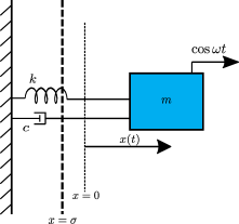
Figure 2: Periodically forced linear oscillator with barrier placed at $x=\sigma$.

$$\ddot{x}+x=\cos{\omega t},$$ (17)

if, $$x(t_{-})=\sigma\mathchar 24635\relax\;\ \dot{x}(t_{+})=-r\dot{x}(t_{-})$$

The undeformable impacting barrier de2004calculation is placed at $x(t_{0})=\sigma$. At the instant of impact $t=t_{0}$, the oscillator undergoes an instantaneous reversal of velocity which is modelled as $\dot{x}(t_{+})=-r\,\dot{x}(t_{-})$ where $t_{+}$ and $t_{-}$ are the instants before and after collision and $r$ depicts the coefficient of restitution. The dynamics of a perturbed trajectory can be expressed in the state-space form and evaluated using Eqs. (7),(12). The accuracy of the nonsmooth mapping of first order is compared with that of the second order. The baseline of the exact values are taken to be the data obtained by numerically integrating two closely spaced trajectories. The integration is performed in Mathematica using its inbuilt ODE solver i.e., NDSolve. For event detection i.e., when $x(t_{-})=\sigma$, Mathematica’s event detection routine is implemented. The results are numerically accurate up to the $15^{th}$ decimal place. The expressions in Eqs. (18) correspond to the approximation in the flight times of the perturbed trajectory to $\Sigma_{2}$ after the primary trajectory has impacted this surface. The entity $\delta_{1}$ in Eq. (18) depicts the linearized expression of Eq. (7), i.e., Eq. (13). The variables $\delta_{2}$ and $\delta_{3}$ in Eq. (18) are obtained from Eq. (7) by expanding the discriminant upto $\mathcal{O}(1)$ and $\mathcal{O}(2)$ respectively. Meanwhile, $\delta_{4}$ is numerically obtained from Eq. (7) considering only the positive root in $\delta$.

$$\delta_{1} =-\frac{y_{1}}{v_{-}},$$ (18a)

$$\delta_{2} =-\frac{y_{1}}{v_{-}+y_{2}},$$ (18b)

$$\delta_{3} =-\frac{y_{1}}{v_{-}+y_{2}}-\frac{(-\sigma+\cos{\omega t_{0}})y_{1}^{2}}{2(v_{-}+y_{2})^{3}},$$ (18c)

$$\delta_{4} =-\frac{v_{-}+y_{2}}{-\sigma+\cos{\omega t_{0}}}$$ (18d)

$$\qquad-\frac{v_{-}+y_{2}}{-\sigma+\cos{\omega t_{0}}}\sqrt{1-2\frac{(-\sigma+\cos{\omega t_{0}})y_{1}}{(v_{-}+y_{2})^{2}}}$$

$y_{i}$ are the components of the perturbed trajectory when Eq. (17) is expressed in the state-space form, i.e. Eq. (1). To demonstrate the accuracy of the proposed higher order corrections to the TDM, the flow of two trajectories, in the phase-space, separated by a perturbation of norm $\lVert\vec{y}\rVert=1$ is shown in Fig. 3. Investigation of trajectories separated by a norm of unit magnitude is necessary. This is because the fundamental solution matrix, which evolves in time to produce state transition matrices, is constructed by considering a unit sphere of perturbed vectors. This ensures that the initial fundamental solution matrix is an identity matrix. The trajectory shown in blue which corresponds to $\omega=2.0$, $\sigma=0.0$ and $r=0.8$ starts from an initial condition after $1000$ impacts to eliminate any transient effects. The perturbed trajectory shown in red evolves obeying the Jacobian of the respective dynamical system. At the instant of impact at $t=t_{0}$, the perturbed trajectory gets mapped in accordance with the defined $\mathcal{O}(1)$ and $\mathcal{O}(2)$ TDM. In principle, from the instant of impact to the instant when $t=t_{0}+\delta$, the perturbed trajectory, if accurately mapped should lie on the discontinuity boundary defined by $H(\vec{x})=0$. In Fig. 3(a) the trajectories at the instant of impact after the application of TDM is shown pictorially when mapped using $\mathcal{O}(1)$ time difference and TDM (i.e., Eq. (13) and Eq. (16)). Fig. 3(b) corresponds to the trajectories after the application of TDM, a time $\delta$ later, i.e., when $t=t_{0}+\delta$. As evident, the mapped perturbed vector does not lie on the discontinuity boundary. Similarly, in Figs. 3(c) - (d) and Figs. 3(e) - (f), the trajectories after impact corresponding to $\mathcal{O}(1)$ time difference, $\mathcal{O}(2)$ TDM (i.e., Eq. (13) and Eq. (12)) and $\mathcal{O}(2)$ time difference, $\mathcal{O}(1)$ TDM (i.e., Eq. (7) and Eq. (16)) is shown respectively. The perturbed trajectory reaches the discontinuity boundary after $t=t_{0}+\delta$ using $\mathcal{O}(2)$ TDM as it should. Thus, it is evident that implementation of the higher order time difference and $\mathcal{O}(2)$ TDM does provide an accurate mapping of perturbed trajectories at the instant of border collision. In Fig. 4, the percentage error in the time estimate $\delta_{i}$s with relation to the numerically computed time is shown. The percent error has been calculated by numerically integrating two closely separated trajectories executing border collision in the state space defined by Eq. (17). Results indicate that the prediction of the flight time $\delta$ using higher order terms is significant in comparison to $\mathcal{O}(1)$. This is because the flight time prediction using $\mathcal{O}(2)$ i.e., $\delta_{4}$ in Eqs. (18), takes into account the functional form of the driving force of the respective PWS system.

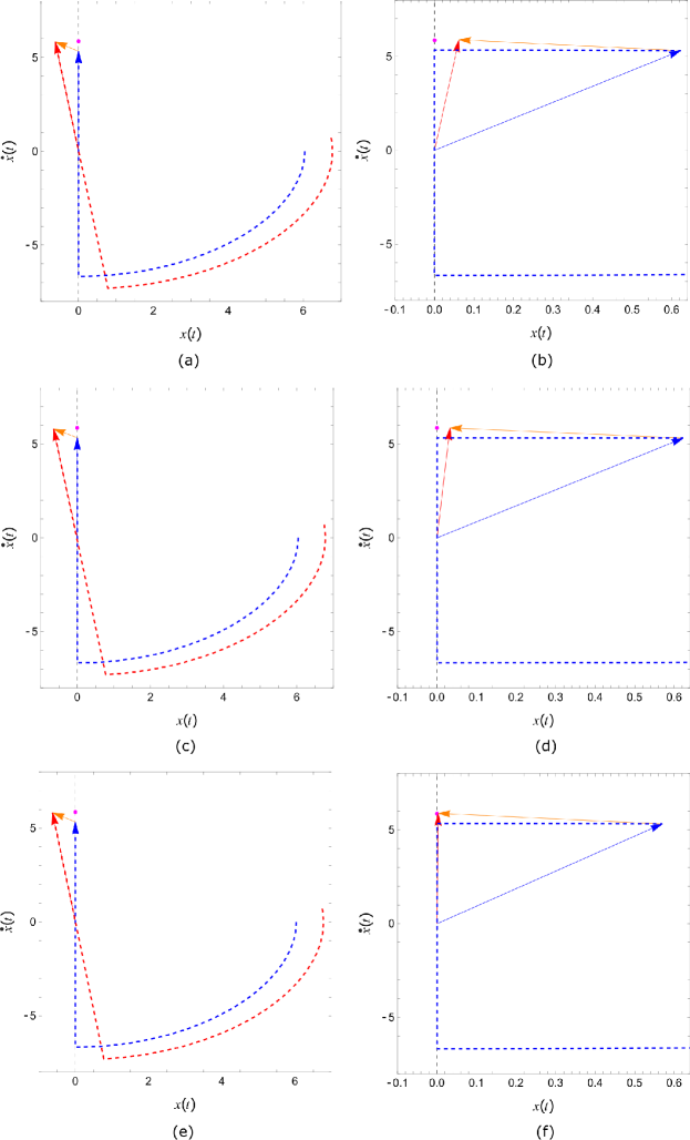
Figure 3: Two trajectories in the phase-space, shown in blue and red dashed lines, separated by a perturbation $\lVert\vec{y}\rVert=1.0$. The magenta colored point is the exact numerical value of where $\vec{x}$ should get mapped to after $t=t_{0}+\delta$. The discontinuity boundary $H(\vec{x})=x-\sigma=0$ is shown as a black dashed line. (a)Trajectories at instant of impact $t=t_{0}$ with $\vec{y}$ mapped using $\mathcal{O}(1)$ saltation terms; see Eq. (16). (b)Trajectories at $t=t_{0}+\delta_{1}$ evaluated using $\mathcal{O}(1)$, i.e., Eq. (13). (c)Trajectories at instant of impact $t=t_{0}$ with $\vec{y}$ mapped using $\mathcal{O}(2)$ Eq. (12) (d)Trajectories at $t=t_{0}+\delta_{1}$ evaluated using $\mathcal{O}(1)$, i.e., Eq. (13) (e)Trajectories at instant of impact $t=t_{0}$ with $\vec{y}$ mapped using $\mathcal{O}(1)$ Eq. (16) (f)Trajectories at $t=t_{0}+\delta_{4}$ evaluated retaining $\mathcal{O}(2)$ terms, i.e., Eq. (7).

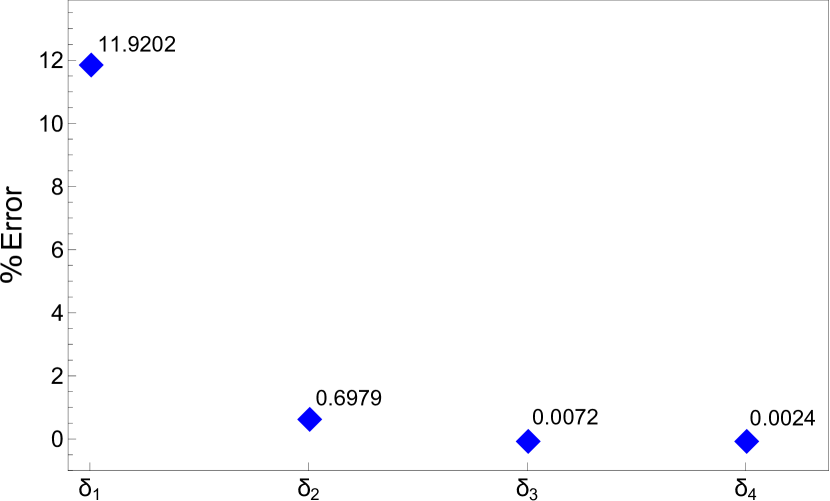
Figure 4: Percent errors in prediction of flight time i.e., $\delta_{i}$s as defined in Eq. (18), in comparison to the numerically obtained flight times. The computations are carried out for forcing frequency, $\omega=2.0$ with barrier at $\sigma=0.0$ and $r=0.8$. The initial separation between trajectories is $\lVert\vec{y}\rVert=0.1$.

In Fig. 5, the error percent in the state variable $\dot{x}$ of a perturbed trajectory getting mapped in state space when the primary trajectory undergoes border collision is shown. $\mathcal{O}(1)$ and $\mathcal{O}(2)$ refers to the mapping of the perturbed trajectory obtained using the linearized saltation matrix presented in Eq. (16) versus the proposed mapping with higher order corrections as defined in Eq. (12). The percent errors are evaluated using combinations of the flight time expressions for $\delta$ as described in Eq. (18) with the orders of mapping of $\vec{x}_{4}$. The numerical values obtained indicate that the error is the least and almost negligible when a combination of $\delta_{4}$ and $\vec{x}_{4}$ from Eq. (12) is used. Thus the proposed higher order corrections significantly improve the analytical estimates when the trajectories at the instant of border collision undergo instantaneous reversals.

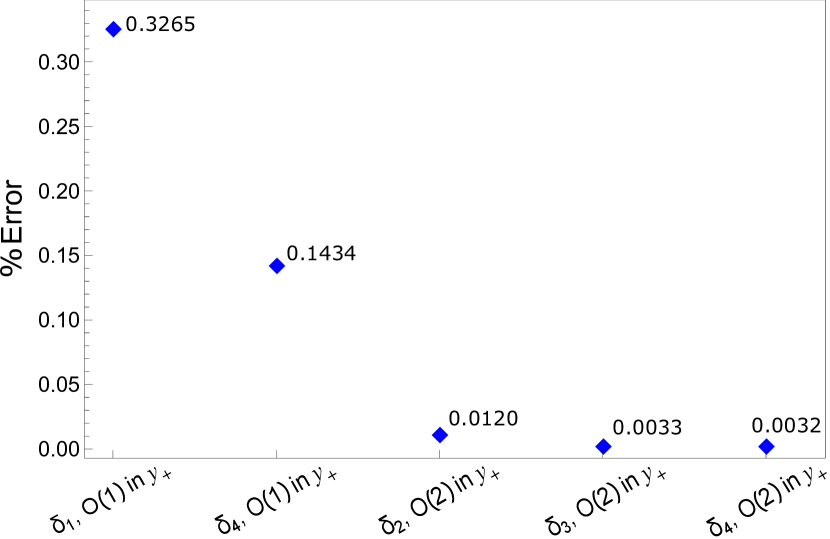
Figure 5: Comparison of errors in predicted $\vec{y}_{+}$ for different combinations of $\delta_{i}$s and $\mathcal{O}(1)$, $\mathcal{O}(2)$ mapping of $\vec{y}_{+}$ with respect to the numerical obtained exact values. Results are shown for $\omega=2.0$, $r=0.8$ and $\sigma=0.0$. Initial separation between trajectories is $\lVert\vec{y}\rVert=0.1$.

In general, PWS systems attains steady state after multiple border collisions. Therefore, errors encountered at every instant of border collision will accumulate after multiple interactions of the trajectory with a discontinuity boundary. This ultimately leads to an incorrect prediction of the steady state. Moreover, for the evaluation of the monodromy matrix numerically, the initial fundamental solution matrix is an identity matrix. This geometrically can be represented by an initial orthogonal set of perturbed vectors lying on a hypersphere of unit radius. The initial trajectories would thus be separated by perturbed vectors on unit norm. In this regime, the evaluation of the state transition matrix using a linearized approach could lead to incorrect TDM of the perturbed vectors. Therefore, in Fig. 6, a comparison of errors in $\dot{x}$ of a perturbed trajectory, introduced at an instant of border collision when $\vec{y}_{+}$ is mapped in accordance to a linearized TDM and with the proposed higher order corrections with varying separation between two adjacent trajectories is shown. The linearized mapping is given by $\delta_{1}$ in Eq. (18) and $S$ in Eq. (16) whereas the $\mathcal{O}(2)$ correction is given by $\delta_{4}$ in Eq. (18) and Eq. (12). The percent error is plotted for varying initial separation between the perturbed trajectory and the primary trajectory of the PWS system at the instant of border collision. Results indicate that the errors introduced in the prediction of the state using the derived TDM is almost nonexistent and therefore can accurately predict the long time dynamics of a PWS systems attaining steady state after multiple border collisions.

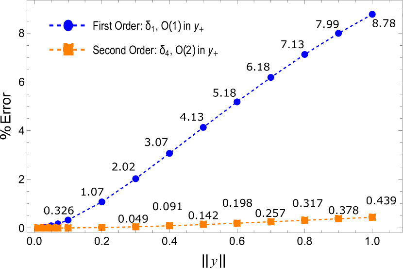
Figure 6: Comparison of percent error in $\dot{x}$ at the instant of border collision when $\vec{y}_{+}$ is mapped using $\mathcal{O}(1)$ vs $\mathcal{O}(2)$ TDM by varying separation between trajectories $\|\vec{y}\|$. Results are shown for $\omega=2.0$, $r=0.8$ and $\sigma=0.0$.

3.2 Pair impact oscillator

For the second representative PWS system, a mechanical oscillator executing border collision with two rigid undeformable barrier is modelled by a pair impact oscillator han1995chaotic ; see Fig. 7. This setup consists of a point mass object placed on a cart executing periodic motion. $x(t)$ and $y(t)$ describes the displacement of the object with respect to the stationary and cart’s frame of reference while $e(t)=\alpha\sin{\omega t}$ describes the periodic motion of the cart excited externally with frequency $\omega$. Hence, we have a relation $x(t)=y(t)+e(t)$ and Eq. (19) describes the dynamics of the point mass object.

$$\ddot{y} =\alpha\omega^{2}\sin{\omega t},$$ (19)

$$\text{if,}\ y(t_{-}) =\pm\frac{\nu}{2}\mathchar 24635\relax\;\ \dot{y}(t_{+})=-r\dot{y}(t_{-})$$

The width of the cart is expressed by $\nu$. Naturally, the motion of this point mass object will be obstructed at either walls of the cart when $y(t_{-})=\pm\frac{\nu}{2}$. Similarly, an instantaneous velocity reversal occurs and is defined in Eq. (19) where $t_{-}$ and $t_{+}$ denote the instant before and after impact. As defined for the impact oscillator, $r$ represents a coefficient of restitution.

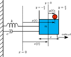
Figure 7: Point mass object placed on a cart excited by harmonic forcing. Impact occurs when $y=\pm\nu/2$.

An implementation of the derived TDM algorithmically to demonstrate the efficiency of higher order corrections is necessary. Therefore, in the succeeding section, the stability analyses for the impact and pair-impact oscillator by investigating the Lyapunov spectrum is presented. Since these representative systems are piece-wise continuous, the derived second order mapping using Eq. (7) and Eq. (12) is implemented. An algorithm to calculate the LE spectrum using the proposed framework is introduced. This methodology is applicable to any generalized PWS hybrid system interacting with a discontinuity transversally. The proposed algorithm integrates any arbitrary PWS system expressed in the state space form and does not require any prior knowledge of the systems analytical solution near the discontinuity boundary.

4 Lyapunov exponents

This section presents the stability analysis of the impact and pair-impact oscillator defined in section 3. The variational equation for each of the representative PWS system is integrated with fixed initial conditions and varying external forcing conditions. When each of these systems encounter a border collision, the perturbed vectors are mapped in the state space using the higher order corrections; see Eqs. (7),(12). To study the accuracy of this method, a stability analysis is carried out by investigating the Lyapunov spectrum. The results are validated by the corresponding stroboscopic bifurcation diagrams. Here, the amplitude of the oscillators at steady state are observed when the forcing frequency is the bifurcation parameter. The Lyapunov characteristic exponent (LE) of a dynamical system measures the exponential divergence of two closely spaced trajectories. For a dynamical system of order $\mathbb{R}^{n}$, the exponential divergence along the $i^{th}$ orthogonal eigenvector is defined as strogatz2018nonlinear

$$\lambda_{i}=\frac{1}{\tau N}\Sigma_{n=1}^{N}\log{\Big{(}\frac{r_{n}}{r_{0}}\Big{)}}.$$ (20)

The $i^{th}$ LE in Eq. (20) is evaluated by measuring the growth of the variation after every time period $\tau=2\pi/\omega$ i.e., in a stroboscopic fashion. Since the parent system is of order $\mathbb{R}^{n}$, there are $n$ independent solutions of the corresponding variational form. Therefore, any arbitrary solution can be decomposed along these $n$ eigenvectors. To measure the $i^{th}$ LE along an eigenvector, a QR decomposition (QRD) is carried out using the Gram-Schmidt process. The process yields $n$ orthogonal perturbed vectors. These orthogonal vectors can be encapsulated in a hypersphere of dimension $n$. The growth or decay of this hypersphere along the trajectory over time is an indicator of the stability of the dynamical system. LE along eigendirection is calculated by numerically integrating each of these orthogonal vectors and measuring the change in magnitude of these vectors after a time interval of $\tau$. $r_{0}$ and $r_{n}$ in Eq. (20) are the initial and final magnitudes of the perturbed vector after elapsed time $\tau$. However, for chaotic systems, the perturbed vectors might quickly diverge from the actual trajectory and the linearized variational form might not be able to capture the actual dynamics of the perturbed trajectory. Therefore, the initial perturbed hypersphere is kept small in its radius centered on the trajectory by using a scaling factor $r_{0}$ in Eq. (20). Furthermore, to obtain accurate values of LE, $\lambda_{i}$ in Eq. (20) has been averaged out over several computations and it is ensured that the actual trajectory is on the invariant set by disregarding the transient cycles of oscillations. The algorithm presented describes the necessary steps in the implementation of this method; see Algorithm 1.

Algorithm 1 Lyapunov exponent for PWS systems using TDM

1. Initialize: $\vec{x}(0)$ ensuring $H(\vec{x}\geq 0)$

2. Initialize: $\omega$ or $\alpha$ $\ignorespaces\triangleright$ Bifurcation parameter

3. Initialize: $\vec{y}_{i}(0)$ for $i\leq n$ using QRD

4. Rescale: $\vec{y}_{i}(0)\leftarrow r_{0}*\vec{y}_{i}(0)$

5. Initialize: $n_{max}$ $\ignorespaces\triangleright$ Maximum allowable impacts

while count $\leq n_{max}$ do

     Integrate: $\dot{\vec{x}}=\vec{F}(\vec{x})$

     if $H(\vec{x})=0$ then $\ignorespaces\triangleright$ Occurrence of border collision

         Evaluate: $\delta$, $\vec{R}(\vec{x})$ and $\vec{y}_{+}$

         Reset Map: $\vec{x}\leftarrow\vec{R}(\vec{x})$

         Reinitialize: $\vec{y}_{i}\leftarrow\vec{y}_{i,+}$ $\ignorespaces\triangleright$ Implement TDM

     end if

     if $\big{(}t\%\frac{2\pi}{\omega}\big{)}=0$ then

         

         if count $\geq n_{max}/2$ then

              Store: $r_{i}\leftarrow\frac{1}{r_{0}}\|\vec{y}_{i}\|$

         end if

         Reinitialize: $\vec{y}_{i}\leftarrow r_{0}*\text{QRD of }\vec{y}_{i}$

     end if

end while

6: Evaluate: $\log_{e}r_{i}$ $\ignorespaces\triangleright$ Store all $log_{e}r_{i}$

7: LE${}_{i}\leftarrow\frac{\omega}{2\pi}*\text{Partial sum of }\log_{e}r_{i}$

8: $\lambda_{i}\leftarrow\langle\text{LE}_{i}\rangle$ $\ignorespaces\triangleright$ Mean of all LEs

4.1 Impact oscillator

The hybrid impact oscillator described in Eq. (17) is investigated for its stability. The external frequency, $\omega$ is taken to be the bifurcation parameter. The exponential divergence between perturbed trajectories is calculated every cycles of $2\pi/\omega$. At first, a hypersphere of radius $r_{0}=0.001$ is initialised. After one cycle of evolution, a QRD and re-scaling in $r_{0}$ is carried out. Figures 8(a) and 8(b) show the phase portraits and the LE spectrum respectively for $\omega=1.0$. Similar plots for $\omega=1.1$ with $r=0.8$ have been presented in Fig. 9. For $\omega=1.0$, the oscillator has a period-2 limit cycle while for $\omega=1.1$, the dynamics in the state space is chaotic. The periodicity of an impact oscillator is computed here as the number of times the trajectory crosses the Poincaré section $\dot{x}=0$, provided $\ddot{x}>0$. The LE spectrum is plotted against the strobe count $\bar{n}$. The largest LE is observed to be positive for $\omega=1.1$. The LEs have been calculated by integrating Eqs. (17) using NDSolve along with the inbuilt event detection functionality in Mathematica. At the instant of impact when $H(\vec{x})=0$, the perturbed trajectory is mapped according to Eqs. (7) and (12) using $\vec{y}_{+}=\vec{x}_{4}-\vec{R}(\vec{x}_{i})$. For the hard barriered vibro-impact oscillator, these expressions are shown in Eq. (21).

$$\delta =-\frac{v_{-}+y_{2}}{-\sigma+\cos{\omega t_{0}}}-\frac{v_{-}+y_{2}}{-\sigma+\cos{\omega t_{0}}}\sqrt{1-2\frac{(-\sigma+\cos{\omega t_{0}})y_{1}}{(v_{-}+y_{2})^{2}}},$$ (21a)

$$\vec{y}_{+} =\begin{bmatrix}y_{1}+\delta v_{-}(1+r)+\delta y_{2}(1-r^{2})+\frac{\delta^{2}}{2}(-\sigma+\cos{\omega t})(1-r)-\delta^{2}r^{2}(-\sigma+\cos{\omega t})\\ -ry_{2}-\delta(-\sigma+\cos{\omega t})(1+r)+\delta y_{1}(1+r)+\delta^{2}(1+r)(v_{-}+\frac{1}{2}\omega\sin{\omega t})\end{bmatrix}$$ (21b)

where $y_{i}$ are the components of the perturbed vector and $v_{-}$ is the velocity, $\dot{x}$ at the instant of impact, $t_{0}$.

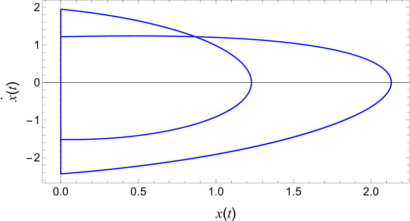
(a)

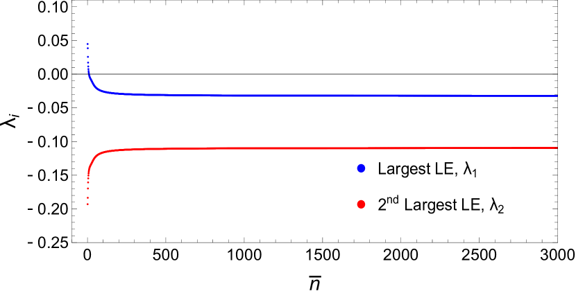
(b)

Figure 8: (a) Phase portrait of the impact oscillator exhibiting period 2 oscillations. (b) The corresponding LE spectrum depicting the presence of a stable orbit. Here, $\omega=1.0$ and $r=0.8$.

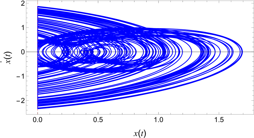
(a)

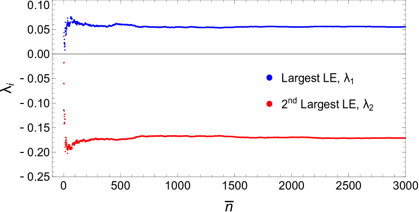
(b)

Figure 9: (a) Phase portrait of an impact oscillator when $\omega=1.1$ and $r=0.8$. (b) The corresponding LE spectrum showing the presence of an unstable orbit.

Fig. 10(a) shows a bifurcation plot of oscillator amplitude plotted against the non-autonomous harmonic frequency $\omega$. The amplitude of the impact oscillator is observed when the condition $\dot{x}=0$ is satisfied at every $\omega$. The integration is performed for a total of $6000$ impacts and amplitudes for the first $3000$ impacts have been discarded to eliminate any transient effects. Fig. 10(b) shows the LE spectrum plotted against $\omega$. It is observed that the LE spectrum is in agreement with the bifurcation plot. Here, the positive values of LE corresponds to chaotic trajectories and the LLE becomes zero at the parameter of occurrence of a period doubling. Dashed vertical lines have been shown in figure for an easy comparison between the bifurcation figure and the corresponding LEs to highlight some of the aperiodic chaotic solutions. Similarly, Fig. 11 and Fig. 12 depict the bifurcation diagrams and the corresponding LE spectrum for $\omega$ ranging between $0.35\leq\omega\leq 1.3$ and $2.5\leq\omega\leq 3.5$ respectively. It is thus verified that the calculated LE spectrums depict the actual underlying behaviour of the steady states.

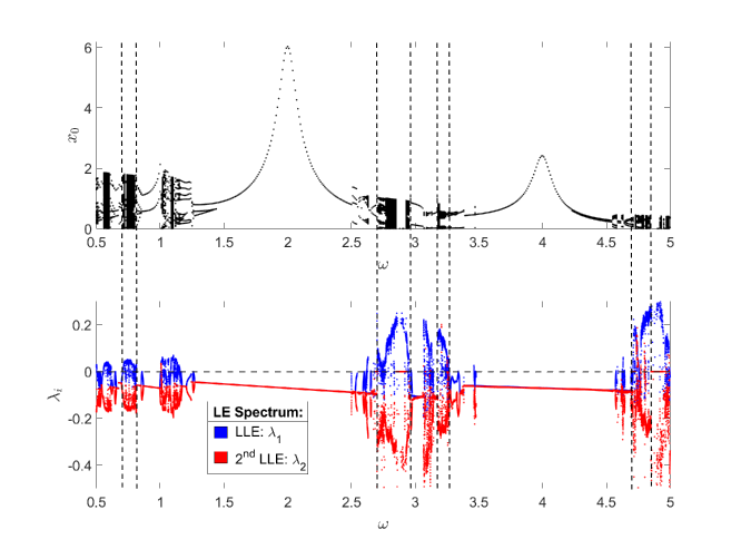
Figure 10: (a) Amplitude $x_{0}$ of the impact oscillator at steady state, i.e., after disregarding 6000 impacts, when $\dot{x}=0$. (b) The corresponding LE spectrum for $0.5\leq\omega\leq 5.0$ and $r=0.8$.

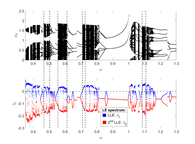
Figure 11: (a) Amplitude $x_{0}$ of the impact oscillator after 6000 impacts when $\dot{x}=0$. (b) LE spectrum for $0.35\leq\omega\leq 1.3$ and $r=0.8$.

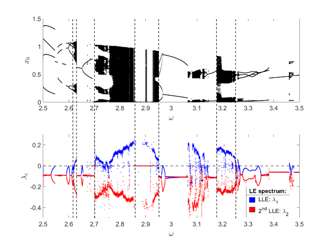
Figure 12: (a) Amplitude $x_{0}$ of the impact oscillator at steady state when $\dot{x}=0$, after 6000 impacts. (b) The corresponding LE spectrum. Here, $2.5\leq\omega\leq 3.5$ and $r=0.8$.

4.2 Pair impact oscillator

Along similar lines, the stability analysis of the pair-impact oscillator described in Sec. 3 is carried out. The cart is assumed to have a width of $\nu=2.0$ and oscillates with a frequency of $\omega=1.0$. The point mass object moves freely on this cart unless it impacts the cart wall at $\nu=\pm\nu/2$. At this instant of impact there is a instantaneous reversal of velocity with a coefficient of restitution $r=0.7$ as defined in Eq. (19). Figures 13 and 14 show the state space trajectories and both the LEs for two values of amplitude $\alpha=1.0$ and $\alpha=1.5$. For $\alpha=1.0$, the orbit is stable with negative LEs while $\alpha=1.5$ results in a chaotic orbit for which the largest LE is positive. For this system, the mapped entities can be analytically expressed as Eq. (22). Here, $y_{i}$ are the components of the perturbed vector and as before $v_{-}$ is the velocity $\dot{x}=0$ at instant of impact, $t_{0}$.

$$\delta =-\frac{v_{-}+y_{2}}{\alpha\omega^{2}\sin{\omega t}}-\frac{v_{-}+y_{2}}{\alpha\omega^{2}\sin{\omega t}}\sqrt{1-2\frac{(\alpha\omega^{2}\sin{\omega t})y_{1}}{(v_{-}+y_{2})^{2}}},$$ (22a)

$$\vec{y}_{+} =\begin{bmatrix}y_{1}+\delta v_{-}(1+r)+\delta y_{2}(1-r^{2})+\frac{\delta^{2}}{2}\alpha\omega^{2}\sin{\omega t}(1-r)-\delta^{2}r^{2}\alpha\omega^{2}\sin{\omega t}\\ -ry_{2}-\delta\alpha\omega^{2}\sin{\omega t}(1+r)-\frac{\delta^{2}}{2}\alpha\omega^{3}\cos{\omega t}(1+r).\end{bmatrix}$$ (22b)

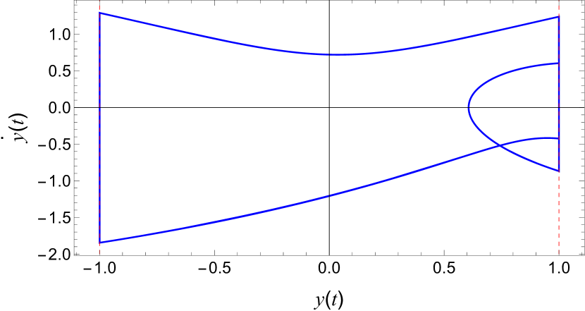
(a)

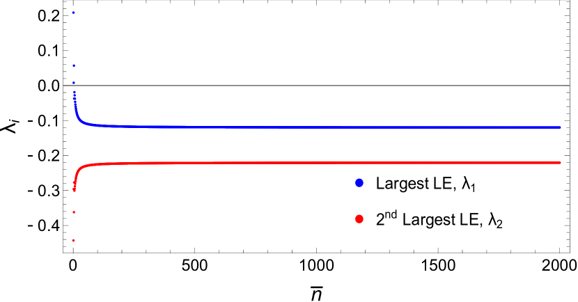
(b)

Figure 13: (a) Phase portrait for a pair impact oscillator describing the dynamics of the point mass. The red dashed lines denote the presence of un-deformable surfaces $\Sigma_{2a}:(y=\nu/2)$ and $\Sigma_{2b}:(y=-\nu/2)$ (b) The corresponding LE spectrum showing a stable orbit when $\alpha=1.0$ with $\omega=1.0$ and $r=0.8$

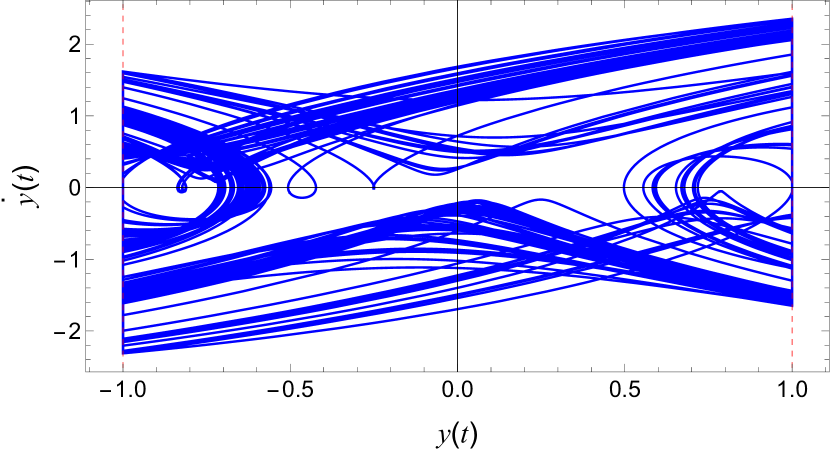
(a)

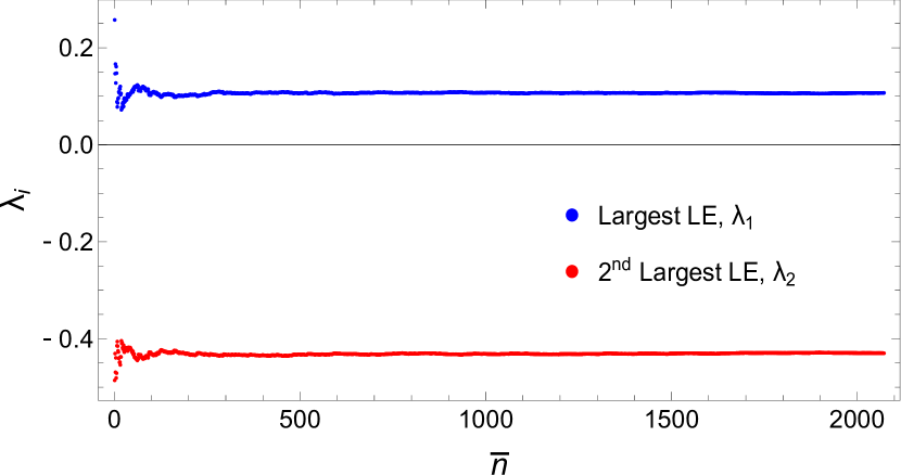
(b)

Figure 14: (a) Parametric plot of $y(t)$ vs $\dot{y}(t)$ in phase space for pair impact oscillator. The red dashed lines denote impacting barriers placed at $\Sigma_{2a}:(y=\nu/2)$ and $\Sigma_{2b}:(y=-\nu/2)$. (b) The corresponding LE spectrum showing the presence of an orbit with positive exponential divergence when $\alpha=1.5$ with $\omega=1.0$ and $r=0.8$.

Now, Fig. 15(a) shows a bifurcation plot where the impact velocity at steady state is plotted against the corresponding oscillation amplitude $\alpha$. For the bifurcation diagram, the velocity of the point mass object $\dot{y}$ is stored at the instant of impact when $y=\pm\nu/2$ for varying $\alpha$. The bifurcation parameter $\alpha$ ranges from $0.5$ to $2.0$. In Fig. 15(b), the LE spectrum against $\alpha$ is shown by integrating for $6000$ impacts. The LEs for the first $3000$ impacts has been discarded in the computations. Positive values of LLEs indicate that the underlying orbit is chaotic for the corresponding oscillation amplitude, $\alpha$.

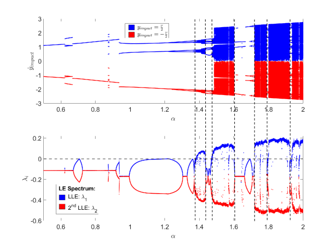
Figure 15: (a) Velocity $\dot{y}$ of steady state pair impact oscillator at instants of impact, i.e., $y=\pm\nu/2$, presented as a function of the forcing amplitude $\alpha$. The first 6000 impacts have been discarded. (b) The corresponding LE spectrum. Here, $0.5\leq\alpha\leq 2.0$, $\omega=1.0$ and $r=0.7$.

5 Floquet multipliers

This section presents an investigation of the stability of attractors in hybrid systems using an eigenvalue analysis on the STM over the stable orbit, also described as the monodromy matrix. According to Floquet theory floquet1883linear , eigenvalues of the monodromy matrix determine the stability of a limit cycle. This analysis is applicable to periodically repetitive dynamics where the Jacobian is periodic. The eigenvalues or characteristic multipliers nayfeh2008applied determine the behaviour in the local linear neighbourhood of steady states in the state space. However for PWS dynamical systems, the monodromy matrix cannot be directly evaluated by integrating the variational form with initial conditions corresponding to an orthogonal basis. This is due to the presence of discrete jumps occurring in the state space near the discontinuity boundaries. A direct implementation of the same leads to incorrect prediction of the state. In order to obtain the correct monodromy matrix, a saltation matrix that defines the state transition between the jumps is to be evaluated. In most studies, the saltation matrix is calculated using the form described in Eq. (16). Retaining $\mathcal{O}(2)$ terms leads to difficulty in writing the saltation terms in the form of a matrix. This is because the perturbed vector $\vec{y}_{+}$ gets mapped according to Eq. (12). A linear transformation between $\vec{y}_{+}$ and $\vec{y}_{-}$ cannot be written in a closed analytical form. To circumvent this representational issue, one can evaluate the saltation in matrix form via a numerical approach, as described below.

For a $n^{th}$ order dynamical system $\vec{x}\in\mathbb{R}^{n}$, the variational equation, whose evolution is governed by terms in the Jacobian (see Eq. (1)), is numerically integrated. The initial conditions are chosen along $n$ orthogonal vectors and the perturbations are represented by $\vec{y}_{i}$. These vectors are expressed in the form of a matrix as

$$\mathbf{Y}_{n\times n}(t) =[\vec{y}_{1}\ \vec{y}_{2}\ \vec{y}_{3}\ldots\vec{y}_{n}],$$ (23)

$$\mathbf{Y}_{n\times n}(0) =\mathbb{I}_{n\times n}$$

The variational equation coupled to the system is integrated up to the instant of impact of the actual trajectory $\vec{x}$. Here, the vectors before and after impact, given by $\mathbf{Y}_{-,impact}$ and $\mathbf{Y}_{+,impact}$ can be expressed as

$$\mathbf{Y}_{+,impact} =\begin{bmatrix}y^{(1)}_{+,1}&\ldots&y^{(1)}_{+,n}\\ \vdots&\ddots&\vdots\\ y^{(n)}_{+,1}&\ldots&y^{(n)}_{+,n}\end{bmatrix}_{n\times n},$$ (24a)

$$\mathbf{Y}_{-,impact} =\begin{bmatrix}y^{(1)}_{-,1}&\ldots&y^{(1)}_{-,n}\\ \vdots&\ddots&\vdots\\ y^{(n)}_{-,1}&\ldots&y^{(n)}_{-,n}\end{bmatrix}_{n\times n}$$ (24b)

where $\vec{y}^{(i)}_{j}$ is the $i^{th}$ component of $j^{th}$ vector. A state transition matrix between perturbed vectors $\vec{y}_{+}$ and $\vec{y}_{-}$ at the instant of impact can be expressed as

$$\mathbf{Y}_{+,impact}=\mathbf{S}_{2}\cdot\mathbf{Y}_{-,impact}$$ (25)

Here, $\mathbf{S}_{2}$ is defined as the saltation matrix for a dynamical system. The subscript 2 denotes the evaluation of the variational form upto $\mathcal{O}(2)$, which is the entity of interest. Alternatively, this saltation matrix can be expressed as

$$\mathbf{S}_{2}=\mathbf{Y}_{+,impact}\cdot\mathbf{Y}_{-,impact}^{-1}$$ (26)

The RHS of Eq. 26 can now be numerically evaluated. Floquet theory states that eigenvalues of the monodromy matrix provide a representation of the local stability of periodic solutions. The theory however is applicable to dynamical systems where the Jacobian matrix has constants as entries or is periodic in time, ensuring that its entries are constant on any lower dimensional section taken along the limit cycle. The two impact oscillators under investigation are non-autonomous, with an external forcing period of $2\pi/\omega$. The periodicity of the underlying attractor is numerically determined by integrating the system until it undergoes $2000$ impacts per impacting surface. The duration between the recurrence of state $\vec{x}$ across a well defined Poincaré section post transience yields the time period of oscillations. Once the time period is calculated, the next step is to evaluate the monodromy matrix, which in this case is decomposed into product of STMs sandwiched between the numerically obtained saltation matrices. The product is taken in the order of occurrence of events, making it essential to evaluate the flight times between impacts as well as the instances of impact. To effectively demonstrate this, a period 2 limit cycle is considered; see Fig. 16.

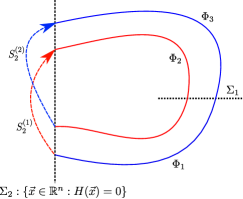
Figure 16: The schematic of a period $2$ limit cycle undergoing two instances of instantaneous reversals at the instants of border collision with $\Sigma_{2}$, depicted as black dashed line. The red solid line corresponds to flow governed by the STM $\Phi_{2}$, the red dashed line corresponds to state transition at the instant of first border collision (using numerically obtained Saltation matrix $S_{2}^{(1)}$), the blue solid line corresponds to flow governed by STM $\Phi_{1}$, the blue dashed line corresponds to state transition at the instant of second impact (using numerically obtained Saltation matrix $S_{2}^{(2)}$).

Here, $\mathbf{\Phi}_{1}$, $\mathbf{\Phi}_{2}$ and $\mathbf{\Phi}_{3}$ are the state transition matrices obtained from the variational equations depicting the transitions from - (1) the Poincaré section $\Sigma_{1}$ to the first encounter with impact surface $\Sigma_{2}$, (2) mapped $\vec{y}_{+}$ to second encounter with $\Sigma_{2}$, (3) mapped $\vec{y}_{+}$ after second encounter with $\Sigma_{2}$ to $\Sigma_{1}$ respectively, eventually completing a limit cycle with time period $T$. $\mathbf{S}^{(1)}_{2}$ and $\mathbf{S}^{(2)}_{2}$ are the saltation matrices, the closed form expressions for which can be obtained from Eq. (26). These saltation terms map the perturbed vectors using Eq. (12) at the instant of impact. Therefore, the monodromy matrix $\mathbf{\Phi}$ for this limit cycle with period $T$, is a resultant of the matrix multiplication given by Eq. (27)

$$\mathbf{\Phi}(T)=\mathbf{\Phi}_{3}\cdot\mathbf{S}^{(2)}_{2}\cdot\mathbf{\Phi}_{2}\cdot\mathbf{S}^{(1)}_{2}\cdot\mathbf{\Phi}_{1},$$ (27)

where the order of matrix dot product is important and the state transition matrices satisfy $\mathbf{\Phi}_{1}(0)=\mathbf{\Phi}_{2}(0)=\mathbf{\Phi}_{3}(0)=\textit{I}_{n\times n}$. For a hybrid dynamical system starting from an arbitrary Poincaré section $\Sigma_{1}$ and executing $n$ impacts with the boundary $\Sigma_{2}$ and converging to an underlying attractor with period $T$, the monodromy matrix thus takes the form

$$\mathbf{\Phi}(T)=\mathbf{\Phi}_{n}\cdot\prod_{i=1}^{n-1}\mathbf{S}_{2}^{i}\cdot\mathbf{\Phi}_{i}$$ (28)

where, $\mathbf{\Phi}_{i}$ is the STM from the Poincaré section $\Sigma_{1}$ to the discontinuous boundary $\Sigma_{2}$. $S^{i}_{2}$ is the saltation matrix evaluated up to $\mathcal{O}(2)$ using Eq. (26) and $\mathbf{\Phi}_{n}$ is the final STM that takes the perturbed trajectory back to the $\Sigma_{1}$ within one time period $T$. In order to evaluate the saltation matrix $S_{2}$ numerically, the initial conditions for the set of orthogonal perturbed vectors in Eq. (23) are chosen as a hypersphere of radius $r_{0}$. A small number is assigned to $r_{0}$ to ensure the perturbations obey the dynamics in the local linear neighbourhood, governed by the Jacobian; see Eqs. (23). Hence, two STMs $\mathbf{Y}_{1}$ and $\mathbf{Y}_{2}$ is defined in Eq. (29) where $\mathbf{Y}_{1}$ evaluates the saltation matrix and $\mathbf{Y}_{2}$ is the STM which maps the perturbed vectors at the instant of border collision.

$$\mathbf{Y}_{1}(0) =r_{0}\textit{I}_{n\times n}\text{, for evaluation of }S_{2}^{i},$$ (29)

$$\mathbf{Y}_{2}(0) =\textit{I}_{n\times n}\text{, for evaluation of }\Phi_{i}$$

The eigenvalues of the monodromy matrix, also known as the Floquet multipliers, are numerically obtained by solving Eq. (28). For a dynamical system of $\mathbb{R}^{n}$, complex conjugate pairs of eigenvalues exist for oscillatory solutions. The magnitude of the eigenvalues is an indicator of the stability of the orbit under consideration. Periodic trajectories yield eigenvalues that lie within the unit circle in the Argand plane. Eigenvalues with magnitude greater than unity denote that perturbed trajectories from the periodic orbit diverges. For aperiodic solutions corresponding to exponentially diverging trajectories, the Floquet multipliers has been calculated from the monodromy matrix for a default time period of $100$s i.e., $\Phi(T=100)$. An algorithmic description for obtaining these Floquet multipliers is provided; see Algorithm 2.

Algorithm 2 Floquet multipliers from monodromy matrix $\mathbf{\phi}$

1. Initialize: $\vec{x}(0)$ ensuring $H(\vec{x})\geq 0$

2. Initialize $\omega$ or $\alpha$ $\ignorespaces\triangleright$ Bifurcation parameter

3. Initialize: $\mathbf{\Phi}=\textit{I}_{n\times n}$, T$=100$, count $=0$

4. Initialize: $n_{max}$ $\ignorespaces\triangleright$ Maximum allowable impacts

while count $\leq$ $n_{max}$ do

     Integrate: $\dot{\vec{x}}=\vec{F}(\vec{x})$

     if $H(\vec{x})=0$ then $\ignorespaces\triangleright$ Occurrence of border collision

         Reset Map: $\vec{x}\leftarrow\vec{R}(\vec{x})$

     end if

     if $\dot{x}=0$ $\&\&$ count $\geq n_{max}/2$ then

         Store $x$, $t$ for evaluation of time period $T$

         $T=\{t\in\mathbb{R}^{1}:x(t+\tilde{n}T)=x(t),\tilde{n}\in\mathbb{I}\}$

     end if

     if count $=$ $n_{max}$ - 100 then $\ignorespaces\triangleright$ Remove transients

         Store: $\vec{x}_{init}$ $\leftarrow\vec{x}(t)$ and $t_{init}\leftarrow t$

     end if

end while

Initialize: $\vec{x}\leftarrow\vec{x}_{init}$ at $t_{init}$ $\ignorespaces\triangleright$ Begin at steady state

Initialize: $r_{0}\ll 1$

Initialize: $\mathbf{Y}_{1}(0)=r_{0}\textit{I}_{n\times n}$ $\ignorespaces\triangleright$ Evaluation of $\mathbf{S}_{2}$

Initialize: $\mathbf{Y}_{2}(0)=\textit{I}_{n\times n}$ $\ignorespaces\triangleright$ Evaluation of $\mathbf{\Phi}_{i}$

while $t_{init}\leq t\leq(t_{init}+T)$ do $\ignorespaces\triangleright$ Integrate over period $T$

     Integrate: $\dot{\vec{x}}=\vec{F}(\vec{x})$

     Integrate: $\dot{\mathbf{Y}_{1}}=(\nabla\vec{F})^{T}\cdot\mathbf{Y}_{1}$

     Integrate: $\dot{\mathbf{Y}_{2}}=(\nabla\vec{F})^{T}\cdot\mathbf{Y}_{2}$

     if $H(\vec{x})=0$ then $\ignorespaces\triangleright$ Occurrence of border collision

         $\mathbf{\Phi}_{i}\leftarrow\mathbf{Y}_{2}$

         $\mathbf{\Phi}\leftarrow\mathbf{\Phi}_{i}\cdot\mathbf{\Phi}$

         Evaluate $\delta$ and $\vec{y}_{+}$ from $\vec{x}_{4}$ for all $\vec{y}_{i}$ $\ignorespaces\triangleright$ TDM

         Evaluate $\mathbf{Y}_{+,impact}$ from $\vec{y}_{+}$

         Define $\mathbf{Y}_{-\text{, impact}}\leftarrow\mathbf{Y}_{1}$

         Evaluate $\mathbf{S}_{2}\leftarrow\mathbf{Y}_{+,impact}\cdot\mathbf{Y}_{-,impact}^{-1}$ $\ignorespaces\triangleright$ saltation matrix

         $\mathbf{\Phi}\leftarrow\mathbf{S}_{2}\cdot\mathbf{\Phi}$

         Reset Map: $\vec{x}\leftarrow\vec{R}(\vec{x})$

         Reinitialize: $\mathbf{Y}_{1}\leftarrow r_{0}\textit{I}_{n\times n}$

         Reinitialize: $\mathbf{Y}_{2}\leftarrow\textit{I}_{n\times n}$

     end if

end while

5. $\mathbf{\Phi}\leftarrow\mathbf{Y}_{2}\cdot\mathbf{\Phi}$ $\ignorespaces\triangleright$ Evaluate monodromy matrix

6. Evaluate eigenvalues of $\mathbf{\Phi}$ to get Floquet multipliers

5.1 Impact oscillator

In this section, the stability analysis of the impact oscillator (see Eq. (17)) is presented. The period of the underlying attractor is evaluated by integrating the system for $2000$ impacts and observing the recurring times of return state $x$ lying on the orbit at section $\dot{\vec{x}}=0$. For the chosen bifurcation parameter $\omega$, the impact oscillator is expressed in the state space form (see Eq. (1)) and is integrated for one period. At the instant of border collision, the saltation matrix $\mathbf{S}_{2}$ (see Eq. (26)) is numerically calculated using TDM defined by Eq. (21) for the impact oscillator. The monodromy matrix is evaluated using Eq. (28) followed by an eigenvalue analysis to determine the stability of the respective limit cycle for a given parameter $\omega$. In Fig. 17, the eigenvalues of $\mathbf{\Phi}(T)$ is shown in the complex plane for external frequency $\omega$ of $1.0$ and $1.1$ respectively.

Figure 17: Floquet multipliers for the impact oscillator showing eigenvalues of a stable and an unstable periodic solution corresponding to $\omega=1.0$ and $\omega=1.1$ in red and blue respectively. The dashed orange circle of unit radius encloses eigenvalues corresponding to stable periodic solutions.

It is observed that the eigenvalues corresponding to $\omega=1.0$ in Fig. 17 are within the unit circle $z=e^{i\theta}$. Therefore it is inferred that the respective limit cycle is stable. This inference is also backed by the phase portrait and the Lyapunov spectrum presented in Fig. 8. However, one of the eigenvalues for $\omega=1.1$ is outside the unit circle and thus the perturbations grow along an eigendirection leading to divergence in trajectories. The underlying chaotic behaviour can be observed in Fig. 9. It is evident that the respective trajectory in the state space is aperiodic while the largest Lyapunov exponent is positive. In Fig. 18(b), the magnitude of both the Floquet multipliers against $\omega$ driving the impact oscillator is shown. A bifurcation diagram of the impact oscillator’s amplitude at steady state against $\omega$ is shown in Fig. 18(a) for reference. Dashed vertical lines have been shown in figure for an easy comparison between the bifurcation figure and the corresponding LEs to highlight some of the aperiodic chaotic solutions The bifurcation parameter $\omega$ ranges from $0.5\leq\omega\leq 5.0$ and the dashed horizontal line in Fig. 18(b) separates the stable region from trajectories which diverge from the periodic limit cycle under investigation. Eigenvalues with norm greater than one correspond to divergent trajectories while those below the dashed line of $\|\rho\|=1$ correspond to stable trajectories for the respective $\omega$. Fig. 19 depicts the real and imaginary part of the Floquet multipliers in the complex plane against $\omega$. The blue cylinder of radius $1$ in figure depicts the stable region. All points within the cylinder represent the occurrence of stable limit cycles while the scattered points lying outside this cylinder with $\|\rho\|\geq 1$ corresponds to diverging trajectories in the state space. Eigenvalues corresponding to unstable trajectories have large values than unity, since in such cases, the trajectories near the periodic limit cycle exponentially diverge. Thus, for visual representation, the eigenvalues corresponding to unstable limit cycles have been scaled down to populate the plot within the defined range; see Figs. 18(b), 19.

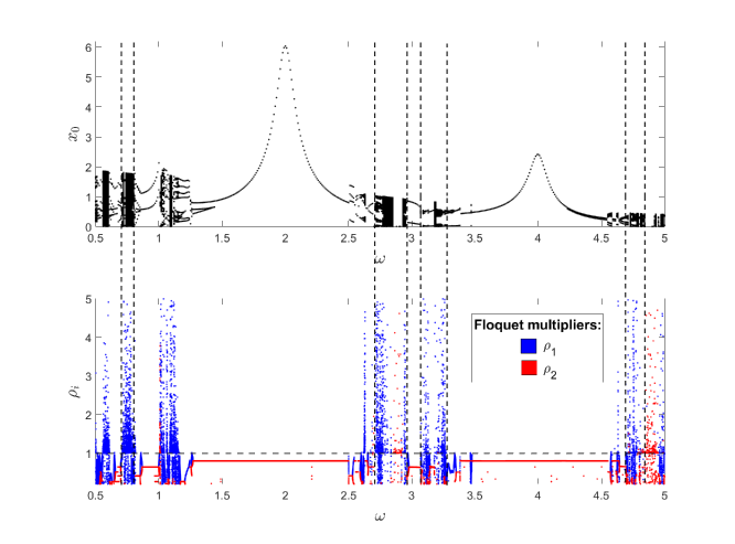
Figure 18: (a) Amplitude $x_{0}$ of the impact oscillator at steady state when $\dot{x}=0$. Here, 6000 impacts have been plotted. (b) The corresponding Floquet multipliers for $0.5\leq\omega\leq 5.0$. Here, $r=0.8$.

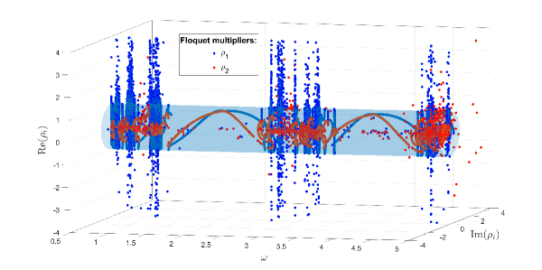
Figure 19: A three dimensional representation of Floquet multipliers of the impact oscillator in the complex plane against the frequency of the harmonic excitation $0.5\leq\omega\leq 5.0$ for $r=0.8$. The blue cylinder of unit radius is the region enclosing Floquet multipliers corresponding to stable periodic solutions.

5.2 Pair impact oscillator

Similarly, the stability analysis of the pair impact oscillator described by Eqs. (19) is discussed in this section. The system is numerically integrated for $4000$ impacts since there are two impacting surfaces $\Sigma_{2}$ at $\pm\nu/2$. The bifurcation parameter is the amplitude $\alpha$ of the external periodic force which drives the cart with frequency $\omega=1.0$. The time period of a periodic limit cycle for a given value of $\alpha$ is evaluated numerically from the recurring time when $\vec{y}$ (see Eq. (19)) intersects the Poincaré section $\vec{y}=0$. The saltation matrix is calculated using the TDM defined in Eq. (22) at the instant of border collisions with either impacting surfaces. The monodromy matrix is evaluated numerically from the deduced STMs and saltation matrices as defined in Eq. (28). The eigenvalues of the obtained monodromy matrix $\mathbf{\Phi}$ are obtained for a given value of $\alpha$, which is then used to deduce the stability of the attractors of the pair impact oscillator.

In Fig. 20, the Floquet multipliers of the pair impact oscillator for forcing amplitude of values $1.0$ and $1.5$ respectively is shown. The eigenvalues for $\alpha=1.0$ is within the unit circle, implying the oscillator is stable, also backed by the observations from the phase-portrait and the respective Lyapunov spectrum; see Fig. 13. However, one of the eigenvalues for $\alpha=1.5$ is outside the unit circle and the corresponding limit cycle shows a diverging trajectory. This is also seen in Fig. 14 where the state space is chaotic and the largest Lyapunov exponent is positive.

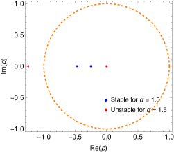
Figure 20: Floquet multipliers for the pair impact oscillator showing eigenvalues of a stable and an unstable periodic solution corresponding to $\alpha=1.0$ and $\alpha=1.5$, in blue and red respectively. The dashed orange circle is of unit radius.

In Fig. 21(b), the magnitude of Floquet multipliers for the pair impact oscillator against the bifurcation parameter $\alpha$ is shown. A bifurcation diagram of the velocity $\dot{\vec{y}}$ at the instant of impact is shown against $\alpha$ for reference in Fig. 21(a). The dashed line where $\|\rho\|=1$ separates the stable periodic limit cycles from the unstable diverging trajectories. $\|\rho\|\geq 1$, in accordance with the Floquet theory, corresponds to values of $\alpha$ for which trajectories near the periodic limit cycle diverges. Figure 22 shows the real and imaginary parts of the Floquet multiplier $\rho_{i}$ for different values of $\alpha$. Eigenvalues that lie outside the cylinder with unit radius correspond to diverging trajectories for the respective $\alpha$. Such eigenvalues with $\|\rho\|>>1$ have been scaled down for representation as described previously.

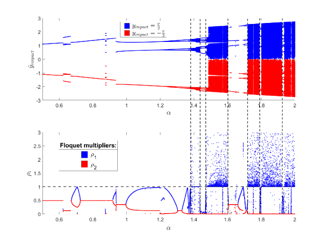
Figure 21: (a) Velocity $\dot{y}$ of the steady state pair impact oscillator at instant of impact, i.e., $y=\pm\nu/2$. The initial 6000 impacts have been disregarded in the computations. (b) The corresponding Floquet multipliers of pair impact oscillator for $0.5\leq\alpha\leq 2.0$, $\omega=1.0$ and $r=0.7$.

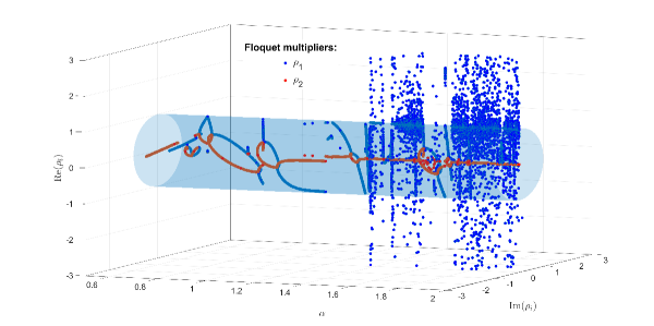
Figure 22: Floquet multipliers of the pair impact oscillator in the complex plane for $0.5\leq\alpha\leq 2.0$, $\omega=1.0$ and $r=0.7$. The blue cylinder of unit radius is the region enclosing Floquet multipliers corresponding to stable periodic solutions for the respective $\alpha$.

6 Conclusion

The stability of PWS systems encountering border collision with immovable barrier is investigated. The following points summarise the key insights presented in this manuscript.

1. For an arbitrary hybrid dynamical system of order $\mathbb{R}^{n}$, a TDM with higher order corrections has been presented. For perturbed trajectories in the vicinity of an invariant set, the expression of the dynamics at the discontinuity boundary has been derived in a closed form. The proposed expression is a higher order extension of the expression present in literature. The proposed closed form expression with higher order corrections to flight times of the perturbed trajectories at the instant of border collision yields better analytical estimates as it incorporates the functional form of the driving force of the respective PWS system. This explicit dependence on the driving force is absent in a linearized approximation. Results implementing the proposed TDM also show improvement over the linearized theory when separation between trajectories is significant.

2. Stability of two representative PWS systems with single and multiple undeformable barriers is investigated. A numerical implementation using higher order TDM to evaluate the LE spectra is demonstrated. The method does not require any prior knowledge of the analytical solution at the instant of border collision, unlike the analytical form for transcendental maps. With the driving force frequency as the bifurcation parameter, bifurcation diagrams are obtained. To corroborate the findings of the underlying attractor from the bifurcation diagram, Lyapunov spectrum has been calculated using the higher order closed form mapping. The Lyapunov spectrum, evaluated at every parameter, is observed to be consistent with the results obtained from the bifurcation analysis. It was observed that the impact oscillators that exhibit the phenomenon of chaos in their state space possess positive largest Lyapunov exponents.

3. A numerical approach to obtain the state transition matrix or saltation matrix at the discontinuity boundary with higher order corrections is proposed. The monodromy matrix for the aforementioned representative systems were obtained by evaluating the STMs and saltation matrices at the instant of border collision. An eigenvalue analysis on the monodromy matrix has been carried out to obtain the respective Floquet multipliers. The observations from the Floquet multipliers and the bifurcation diagram show remarkable correspondence.

Declarations

The authors acknowledge the support of UCD Energy Institute, University College Dublin, Ireland; Science Foundation Ireland, Grant/Award Number: RC2302_2; SIRMA (Strengthening Infrastructure Risk Management in the Atlantic Area) Project, Grant/Award Number: EAPA_826/2018; IReL

Conflict of interest

The authors declare that they have no conflict of interest.

Availability of data

Not applicable.

Availability of code

All codes implemented in this paper is available upon request from the corresponding author.

References

- \bibcommenthead
- (1) Nayfeh, A.H., Balachandran, B.: Applied Nonlinear Dynamics: Analytical, Computational, and Experimental Methods. John Wiley & Sons, ??? (2008)
- (2) Van Der Schaft, A.J., Schumacher, J.M.: An Introduction to Hybrid Dynamical Systems vol. 251. Springer, ??? (2000)
- (3) Bernardo, M., Budd, C., Champneys, A.R., Kowalczyk, P.: Piecewise-smooth Dynamical Systems: Theory and Applications vol. 163. Springer, ??? (2008)
- (4) Di Bernardo, M., Hogan, S.: Discontinuity-induced bifurcations of piecewise smooth dynamical systems. Philosophical Transactions of the Royal Society A: Mathematical, Physical and Engineering Sciences 368(1930), 4915–4935 (2010)
- (5) Chin, W., Ott, E., Nusse, H.E., Grebogi, C.: Grazing bifurcations in impact oscillators. Physical Review E 50(6), 4427 (1994)
- (6) Jiang, H., Chong, A.S., Ueda, Y., Wiercigroch, M.: Grazing-induced bifurcations in impact oscillators with elastic and rigid constraints. International Journal of Mechanical Sciences 127, 204–214 (2017)
- (7) Pavlovskaia, E., Wiercigroch, M., Grebogi, C.: Two-dimensional map for impact oscillator with drift. Physical Review E 70(3), 036201 (2004)
- (8) Simpson, D.J., Avrutin, V., Banerjee, S.: Nordmark map and the problem of large-amplitude chaos in impact oscillators. Physical Review E 102(2), 022211 (2020)
- (9) Piiroinen, P.T., Virgin, L.N., Champneys, A.R.: Chaos and period-adding; experimental and numerical verification of the grazing bifurcation. Journal of Nonlinear Science 14(4), 383–404 (2004)
- (10) Oestreich, M., Hinrichs, N., Popp, K.: Bifurcation and stability analysis for a non-smooth friction oscillator. Archive of Applied Mechanics 66(5), 301–314 (1996)
- (11) Oestreich, M., Hinrichs, N., Popp, K., Budd, C.: Analytical and experimental investigation of an impact oscillator. In: International Design Engineering Technical Conferences and Computers and Information in Engineering Conference, vol. 80425, pp. 01–15008 (1997). American Society of Mechanical Engineers
- (12) Popp, K., Oestreich, M., Hinrichs, N.: Numerical and experimental investigation of nonsmooth mechanical systems. In: IUTAM Symposium on New Applications of Nonlinear and Chaotic Dynamics in Mechanics, pp. 293–302 (1999). Springer
- (13) Shaw, S.W., Holmes, P.: A periodically forced piecewise linear oscillator. Journal of sound and vibration 90(1), 129–155 (1983)
- (14) Fredriksson, M.H., Nordmark, A.B.: On normal form calculations in impact oscillators. Proceedings of the Royal Society of London. Series A: Mathematical, Physical and Engineering Sciences 456(1994), 315–329 (2000)
- (15) Rounak, A., Gupta, S.: Bifurcations in a pre-stressed, harmonically excited, vibro-impact oscillator at subharmonic resonances. International Journal of Bifurcation and Chaos 30(08), 2050111 (2020)
- (16) Oseledec, V.I.: A multiplicative ergodic theorem. liapunov characteristic number for dynamical systems. Trans. Moscow Math. Soc. 19, 197–231 (1968)
- (17) Pesin, Y.B.: Characteristic lyapunov exponents and smooth ergodic theory. Russian Mathematical Surveys 32(4), 55 (1977)
- (18) Benettin, G., Galgani, L., Giorgilli, A., Strelcyn, J.-M.: Lyapunov characteristic exponents for smooth dynamical systems and for hamiltonian systems; a method for computing all of them. part 1: Theory. Meccanica 15(1), 9–20 (1980)
- (19) Bennetin, G., Galgani, L., Giorgilli, A., Strelcyn, J.-M.: Lyapunov characteristic exponents for smooth dynamical systems and for hamiltonian systems: A method for computing all of them. part 2: Numerical application. Meccanica 15(1), 21–30 (1980)
- (20) Benettin, G., Galgani, L., Strelcyn, J.-M.: Kolmogorov entropy and numerical experiments. Physical Review A 14(6), 2338 (1976)
- (21) Termonia, Y.: Kolmogorov entropy from a time series. Physical Review A 29(3), 1612 (1984)
- (22) Floquet, G.: On linear differential equations with periodic coefficients. In: Annales Scientifiques de l’École Normale Supérieure, vol. 12, pp. 47–88 (1883)
- (23) Coleman, M.J., Chatterjee, A., Ruina, A.: Motions of a rimless spoked wheel: a simple three-dimensional system with impacts. Dynamics and stability of systems 12(3), 139–159 (1997)
- (24) Leine, R.: Non-smooth stability analysis of the parametrically excited impact oscillator. International Journal of Non-Linear Mechanics 47(9), 1020–1032 (2012)
- (25) Lamba, H., Budd, C.: Scaling of lyapunov exponents at nonsmooth bifurcations. Physical Review E 50(1), 84 (1994)
- (26) Mandal, K., Chakraborty, C., Abusorrah, A., Al-Hindawi, M., Al-Turki, Y., Banerjee, S.: An automated algorithm for stability analysis of hybrid dynamical systems. The European Physical Journal Special Topics 222(3), 757–768 (2013)
- (27) Rosenstein, M.T., Collins, J.J., De Luca, C.J.: A practical method for calculating largest lyapunov exponents from small data sets. Physica D: Nonlinear Phenomena 65(1-2), 117–134 (1993)
- (28) Wolf, A., Swift, J.B., Swinney, H.L., Vastano, J.A.: Determining lyapunov exponents from a time series. Physica D: nonlinear phenomena 16(3), 285–317 (1985)
- (29) De Souza, S.L., Caldas, I.L.: Calculation of lyapunov exponents in systems with impacts. Chaos, Solitons & Fractals 19(3), 569–579 (2004)
- (30) Jin, L., Lu, Q.-S., Twizell, E.: A method for calculating the spectrum of lyapunov exponents by local maps in non-smooth impact-vibrating systems. Journal of sound and Vibration 298(4-5), 1019–1033 (2006)
- (31) Stefanski, A.: Estimation of the largest lyapunov exponent in systems with impacts. Chaos, Solitons & Fractals 11(15), 2443–2451 (2000)
- (32) Stefański, A., Kapitaniak, T.: Estimation of the dominant lyapunov exponent of non-smooth systems on the basis of maps synchronization. Chaos, Solitons & Fractals 15(2), 233–244 (2003)
- (33) Stefanski, A., Dabrowski, A., Kapitaniak, T.: Evaluation of the largest lyapunov exponent in dynamical systems with time delay. Chaos, Solitons & Fractals 23(5), 1651–1659 (2005)
- (34) Balcerzak, M., Dabrowski, A., Blazejczyk–Okolewska, B., Stefanski, A.: Determining lyapunov exponents of non-smooth systems: Perturbation vectors approach. Mechanical Systems and Signal Processing 141, 106734 (2020)
- (35) Dabrowski, A.: Estimation of the largest lyapunov exponent from the perturbation vector and its derivative dot product. Nonlinear Dynamics 67(1), 283–291 (2012)
- (36) Müller, P.C.: Calculation of lyapunov exponents for dynamic systems with discontinuities. Chaos, Solitons & Fractals 5(9), 1671–1681 (1995)
- (37) Li, T., Lamarque, C.-H., Seguy, S., Berlioz, A.: Chaotic characteristic of a linear oscillator coupled with vibro-impact nonlinear energy sink. Nonlinear Dynamics 91(4), 2319–2330 (2018)
- (38) Yin, S., Wen, G., Xu, H., Wu, X.: Higher order zero time discontinuity mapping for analysis of degenerate grazing bifurcations of impacting oscillators. Journal of Sound and Vibration 437, 209–222 (2018)
- (39) Budd, C., Dux, F., Cliffe, A.: The effect of frequency and clearance variations on single-degree-of-freedom impact oscillators. Journal of sound and vibration 184(3), 475–502 (1995)
- (40) Acary, V.: Higher order schemes for nonsmooth mechanical systems. In: 12th Seminar” NUMDIFF” on Numerical Solution of Differential and Differential-Algebraic Equations (2009)
- (41) Awrejcewicz, J., Lamarque, C.-H.: Bifurcation and Chaos in Nonsmooth Mechanical Systems vol. 45. World Scientific, ??? (2003)
- (42) Han, R., Luo, A., Deng, W.: Chaotic motion of a horizontal impact pair. Journal of Sound and Vibration 181(2), 231–250 (1995)
- (43) Strogatz, S.H.: Nonlinear Dynamics and Chaos: with Applications to Physics, Biology, Chemistry, and Engineering. CRC press, ??? (2018)