The U.S. Naval Observatory VLBI Spectroscopic Catalog

Remington O. Sexton U.S. Naval Observatory, 3450 Massachusetts Ave NW, Washington, DC 20392-5420, USA Department of Physics and Astronomy, George Mason University, 4400 University Dr, Fairfax, VA 22030-4444, USA Nathan J. Secrest U.S. Naval Observatory, 3450 Massachusetts Ave NW, Washington, DC 20392-5420, USA Megan C. Johnson U.S. Naval Observatory, 3450 Massachusetts Ave NW, Washington, DC 20392-5420, USA Bryan N. Dorland U.S. Naval Observatory, 3450 Massachusetts Ave NW, Washington, DC 20392-5420, USA

Abstract

Despite their importance for astrometry and navigation, the active galactic nuclei (AGNs) that comprise the International Celestial Reference Frame (ICRF) are relatively poorly understood, with key information such as their spectroscopic redshifts, AGN spectral type, and emission/absorption line properties generally missing from the literature. Using updated, publicly available, state-of-the-art spectroscopic fitting code optimized for the spectra of AGNs from low to high redshift, we present a catalog of emission line and spectral continuum parameters for 1,014 unique ICRF3 objects with single-fiber spectra from the Sloan Digital Sky Survey DR16. We additionally present black hole virial mass scaling relationships that use H $\alpha$ -, H $\beta$ -, Mg II-, and C IV-based line widths, all consistent with each other, which can be used in studies of radio-loud objects across a wide range of redshifts, and we use these scaling relationships to provide derived properties such as black hole masses and bolometric luminosities for the catalog. We briefly comment on these properties for the ICRF objects, as well as their overall spectroscopic characteristics.

^†^†facilities: VLBA, SDSS^†^†software: Astropy (Astropy Collaboration et al., 2013, 2018), topcat (Taylor, 2005), badass (Sexton et al., 2021), aips

1 Introduction

Since its adoption more than two decades ago, efforts to build the International Celestial Reference Frame (ICRF; Ma et al., 1998) have led to cataloging the celestial coordinates of thousands of compact extragalactic radio sources across the sky, which are powered by active galactic nuclei (AGNs). Decades of very long baseline interferometry (VLBI) observations and careful selection of sources for the ICRF has resulted in an unprecedented increase in accuracy and precision in the fields of deep space and terrestrial navigation, geodesy, and studies of various astrophysical phenomena.

The adoption of a reference frame based on extragalactic sources was first mandated by the International Astronomical Union (IAU) in 1991. This reference frame, based on extragalactic radio observations using dual-frequency 2.3 and 8.4 GHz (S/X band) VLBI, was recommended to the IAU as the realization of the International Celestial Reference System (ICRS; Arias et al., 1995), and is defined using a set of sources carefully selected for precision and uniformity across the sky. The IAU formally adopted the ICRF as part of the ICRS to replace the stellar-based Fifth Fundamental Catalog of Stars (FK5; Fricke et al., 1988) on 1 January 1998.

With the advent of the National Radio Astronomy Observatory’s Very Long Baseline Array (VLBA; Napier et al., 1994), astrometric measurements of quasars became very efficient, resulting in a more-than five-fold increase in the number of VLBI sources by the mid 2000s, prompting the production of the second realization of the ICRF. ICRF2 (Fey et al., 2015) was constructed at S/X bands using a total of 3,414 objects, 295 of which are classified as “defining sources” and set the quasi-inertial barycenter frame of reference. These defining sources were selected to have the optimal astrometric precision and minimal source structure.

The current ICRF, ICRF3, incorporates additional VLBI observations, and accounts for the galactocentric acceleration of the solar system (Titov et al., 2011), greatly improving accuracy. ICRF3 has 4,536 sources at S/X, with 303 defining sources chosen to prioritize isotropy, and includes 824 objects observed at 24 GHz (K band) and 678 objects observed with dual-frequency 8.4 and 32 GHz (X/Ka band), making ICRF3 the first multi-frequency celestial reference frame.

Despite their foundational importance to astronomy and geodesy, relatively little is known about the intrinsic properties of the sources that make up the ICRF, such as black hole (BH) masses, bolometric luminosities, Eddington ratios, host galaxy types, and stellar masses, other than properties derived directly from radio observations. Many sources exhibit significant source structure at VLBI resolution, likely caused by the presence of relativistic jets commonly found in radio-selected AGNs and quasars (Blandford et al., 2019). Positional offsets between the VLBI radio and optical positions of ICRF sources, initially detected prior to Gaia by multiple groups (da Silva Neto et al., 2002; Assafin et al., 2013; Orosz & Frey, 2013; Zacharias & Zacharias, 2014), have been a subject of ongoing study (Mignard et al., 2016; Kovalev et al., 2017; Petrov & Kovalev, 2017; Makarov et al., 2019), and observing programs to understand the astrophysical nature of these offsets are underway (Zacharias et al., 2020). To date, there is evidence that suggests that off-center optical AGN jets are a significant contributor to observed radio-optical offsets (Petrov et al., 2019; Plavin et al., 2019).

Moreover, AGNs and quasars can be some of the most persistently variable objects in the universe (e.g., Ulrich et al., 1997), and exhibit an enormous range of morphologies and spectral energy distributions that change with time. In principle, reference frame objects that exhibit positional stability over one epoch may change significantly in the next epoch, so cataloging objects for the ICRF is not a “one and done” process: objects must be physically characterized and monitored if the ICRF is to become a truly multi-wavelength CRF that is stable and accurate across epochs. It is therefore necessary to have an in-depth understanding of the astrophysical properties of these objects, so as to minimize the impact of the peculiarities of AGNs on the accuracy of the ICRF. Understanding the relevant physics of AGNs and their environments is one of the guiding principles of the Fundamental Reference Frame AGN Monitoring Experiment (FRAMEx: Dorland et al., 2020; Fischer et al., 2021; Fernandez et al., 2022).

While there have been systematic programs to concatenate catalog photometry and redshifts of nearly all ICRF objects (e.g., Malkin, 2018), relatively few ICRF objects have been spectroscopically characterized (e.g., Titov et al., 2017), and efforts have mainly focused on determination of redshift (e.g., Titov & Malkin, 2009). Optical spectra contain an abundant amount of information regarding the physical processes powering AGNs and quasars. Most notable are the presence of permitted Balmer emission features broadened by the bulk motions of gas orbiting the BH, from which we can estimate BH mass (Peterson, 2004), and the apparent flux ratio of permitted emission lines of a particular ionized species can give a direct measure of the line-of-sight (LOS) AGN obscuration. Additionally, the narrow forbidden emission lines of AGNs and quasars can exhibit line profile asymmetries indicative of ionized gas outflows (Nelson & Whittle, 1996), which can provide insight into how the AGN may be interacting with its host galaxy. Properties of the host galaxy can also be inferred from the presence of stellar absorption features to estimate stellar kinematics (Greene & Ho, 2006). Most, if not all, of these intrinsic properties are unknown for ICRF sources but can be estimated via spectroscopy.

In this work, we produce a catalog of spectral properties for ICRF3 sources with spectra available from the Sloan Digital Sky Survey (SDSS) Data Release 16 (DR16; Blanton et al., 2017), and provide value-added properties such as BH masses and bolometric luminosities. In producing this catalog, we have additionally derived new BH virial mass scaling relationships that will be of value for work on radio-loud AGNs, and we have updated the spectral-fitting code of Sexton et al. (2021) to handle high-redshift and radio loud objects. In Section 2 we describe the SDSS DR16 spectroscopic data used in this work. Section 3 provides a detailed description of the spectral code updates, fitting algorithm, strategy, model implementation, and quality metrics used for our sample. Section 4 details the calculation of derived properties such as luminosities, broad emission line widths, and BH mass, as well as the relevant relations between these quantities. We briefly discuss the general spectroscopic properties of ICRF3 objects in Section 5. Finally, in Section 6 we describe the structure, proper usage, caveats, and availability of the catalog for the astronomical community.

Where distances are employed, we use a flat $\Lambda{\textrm{CDM}}$ cosmology with $H_{0}=70$ km s^-1 Mpc^-1 and $\Omega_{\mathrm{m}}=0.3$ . Specific ICRF3 sources are referenced by their IERS designation.

2 Data

Optical spectra for ICRF3 sources were obtained from the SDSS DR16 (Blanton et al., 2017), given its large availability of calibrated AGN and quasar spectra and large wavelength and sky coverage. The original SDSS spectroscopic survey (York et al., 2000) employed spectral fiber apertures with $3\arcsec$ diameter and an observed wavelength coverage from 3800Å to 9200Å. The Baryon Oscillation Spectroscopic Survey (BOSS; Dawson et al., 2013) and extended BOSS (eBOSS; Dawson et al., 2016) introduced in SDSS-III (Eisenstein et al., 2011), employed a $2\arcsec$ diameter fiber with a slightly larger wavelength coverage from 3650Å to 10,400Å. While the main SDSS, BOSS, and eBOSS programs focus primarily on extragalactic sources and avoid the galactic disk, the Sloan Extension for Galactic Understanding and Exploration (SEGUE; Yanny et al., 2009) program probes the Milky way disk and halo stars to obtain stellar parameters, and occasionally observes background extragalactic sources. All SDSS spectra are logarithmically re-binned (Tonry & Davis, 1979) such that each pixel corresponds to a constant velocity of $\sim 69$ km s^-1 in the observed frame.

We cross-matched 4,536 ICRF3 source coordinates with the specObj-dr16.fits table, using a $1\farcs 5$ match tolerance, resulting in 1,559 matches, of which 11 spectra contained no data and were removed from the sample. Of the remaining 1,548 spectra, 534 are repeat observations of the unique set of 1,014 sources, which will be the subject of a future multi-epoch study. To ensure that the best version of each duplicate spectrum was fit, we prioritized available wavelength coverage, which favored BOSS spectra over SDSS spectra.

The sample of unique ICRF3 sources consists of 1,014 SDSS spectra from both the SDSS and BOSS spectrographs, and were observed in various programs including the original SDSS (355), BOSS (383), eBOSS (263), SEGUE1 (7), and SEGUE2 (6).

These individual survey programs cover an area of sky of approximately 14,555 square degrees, predominantly in the northern hemisphere and largely avoiding the Galactic plane, whereas the ICRF3 spans the full sky by design. The area surveyed by the SDSS therefore allows only $\sim 1600$ ICRF3 objects, or $35\%$ of all ICRF3 objects, to be potentially observed within the SDSS footprint. The 1,014 available spectra therefore amounts to $63\%$ of observable ICRF3 sources, or $22\%$ of all ICRF3 sources, with SDSS. The limiting magnitude for our sample is $i_{\rm{PSF}}=20.6$ , which is consistent with the $i_{\rm{PSF}}=20.2$ limiting magnitude for quasar target selection for the SDSS spectrograph. Objects observed using the more-sensitive BOSS spectrograph are limited to $i_{\rm{PSF}}=22.1$ .

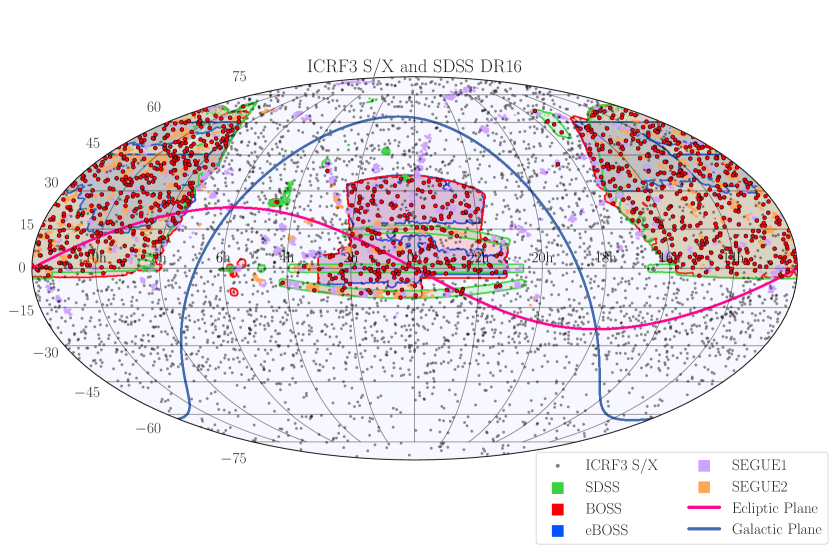
Figure 1 shows the Mollweide projection of all 4,536 S/X sources from ICRF3 from Charlot et al. (2020) with the sky coverage of various SDSS programs from which ICRF3 spectra are obtained. Of the 1,014 unique ICRF3 sources, 58 (5.7%) are defining sources and the remaining 956 objects (94.3%) are densifying sources.

Visual inspection of all objects with the specObj ZWARNING flag set to $>0$ (indicating a potential issue in the pipeline redshift determination) revealed 121 sources with no visible emission or absorption line features from which a redshift could be determined and therefore cannot be fit. These featureless objects are flagged as “featureless” in the catalog.

Twenty-two spectra with $\texttt{ZWARNING}>0$ were determined to have redshifts suitable for fitting purposes. Additionally, seven spectra were determined to have incorrect redshifts, which were corrected using visual inspection using any visible emission or absorption features. Finally, one spectrum (IERS 1048+470) appears to be contaminated by an foreground star in SDSS imaging, producing a unidentifiable spectrum from which no redshift could be determined.

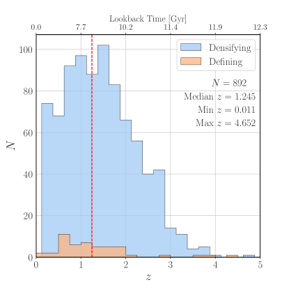
The final sample consists of 892 unique ICRF3 spectra with accurate redshift determinations suitable for fitting (19.7%). This consists of 48 (5.4%) defining and 844 (94.6%) densifying sources with a median redshift of 1.245. Figure 2 shows the redshift distribution of the final fitted sample.

Refer to caption — Figure 1: The Mollweide projection of all 4,536 S/X ICRF3 sources from Charlot et al. (2020). Outlined regions correspond to various SDSS programs from which SDSS spectra of ICRF3 sources are obtained. The 1,014 ICRF3 sources with available spectra are shown as red points.

3 Methods

3.1 Spectral Fitting

The fitting of all spectra is performed using the Bayesian AGN Decomposition Analysis for SDSS Spectra (BADASS¹¹1https://github.com/remingtonsexton/BADASS3; Sexton et al., 2021) software, which is written in Python and specifically designed for fitting AGNs and quasars. The BADASS software has been recently upgraded to allow for the fitting and analysis of high-redshift spectra specific to the needs of the ICRF3 spectroscopic sample, and we provide a brief description of these relevant upgrades.

The original release of BADASS was designed for rest-frame optical SDSS spectra, specifically to model the regions spanning 3500 Å to 7000 Å, and was limited by the available coverage of empirical stellar templates libraries used to simultaneously model the stellar line-of-sight velocity distribution (LOSVD). In order to be able to model the spectra of ICRF3 objects, the majority of which have a $z>1$ , significant modifications and additions to the fitting model were made. These include models for the Balmer pseudo-continuum (Grandi, 1982; Wills et al., 1985) as well as an empirical UV iron template (Vestergaard & Wilkes, 2001), both of which are discussed in further detail in Section 3.3. Additional line profile shapes such as pseudo-Voigt and Gauss-Hermite were added for increased flexibility in modelling broad emission line profiles typically seen in Mg II and C IV. The largest structural change to the algorithm was a complete overhaul of the BADASS framework to allow for easy customization emission lines and the addition of optional soft and hard constraints on emission line parameters. A complete description of all new additions and features to BADASS will be provided in a future manuscript.

The BADASS fitting algorithm relies on the same Bayesian principles outlined in Sexton et al. (2021), with posterior sampling performed using the affine-invariant Markov-Chain Monte Carlo (MCMC) sampler emcee (Foreman-Mackey et al., 2019). A preliminary maximum-likelihood fit to the data is performed to obtain initial parameter values using a normal (Gaussian) likelihood distribution. Flat priors with liberal bounds are initialized for all fitted parameters. A final fit to the data is performed using MCMC to obtain robust uncertainty estimates on all parameters. We do not utilize the built-in autocorrelation analysis functionality of BADASS, since the majority of our parameters are those of emission lines, which nominally converge in under 1000 iterations depending on their signal-to-noise (S/N). We instead perform a maximum of 2500 iterations of MCMC sampling with 100 walkers per parameter and use the final 1000 iterations (1500 burn-in) for the posterior distributions, from which the median (50^th percentile) of the distribution is considered the best-fit values to our parameters, and the 16^th and 84^th percentiles of the distributions are used as the lower- and upper-bound $1\sigma$ uncertainties on each parameter.

Prior to fitting, BADASS performs preliminary data preparation on SDSS spectra, which includes the correction for Galactic extinction. Conversion to rest frame is performed using the redshift determined by the SDSS pipeline except in the seven cases where the redshift was determined to be incorrect, for which we determined the correct redshift using visual inspection. We used the extinction map of Schlafly & Finkbeiner (2011) and corrected using a Cardelli et al. (1989) extinction law assuming an $R_{V}=3.1$ . BADASS does not fit and subtract off any spectral components as a preliminary step to measuring other components such as emission lines, and instead fits all components simultaneously in order to properly constrain their relative contributions and covariances.

In the following subsections, we describe the fitting strategy implemented to fit the ICRF3 spectra, with particular attention given to regions that are important for deriving virial BH masses from broad emission line features and continuum luminosities.

3.2 Fitting Regions

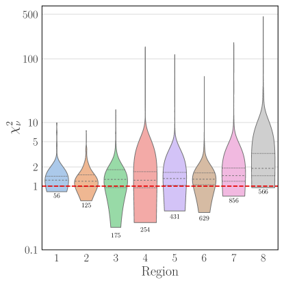
To facilitate the detailed fitting of all ICRF3 spectra, we divide each spectrum into eight fitting regions that span the entire optical and near-UV wavelength coverage of the SDSS and BOSS. The availability of these regions in each spectrum is dependent on the redshift of each object, and therefore not all spectra have data in each region. A description of these fitting regions and their wavelength ranges is shown in Table 1.

Fitting regions are chosen based on available spectral features as a means to limit the number of free parameters in the fit to reduce computation time. Fitting regions, as opposed to full-spectrum fitting, also reduces the chance that a poorly fit region of the spectrum not described by our model (such as poorly subtracted skylines) adversely affects the overall fit. We make an exception for the fitting of continuum quantities (described in Section 3.3), since continuum components (such as power-law, Balmer, and host galaxy continuum) can span multiple regions, and thus we use the entire available spectrum to properly constrain their respective parameters.

To avoid excessive noise at the edges of SDSS spectra, we require that the spectrum have a minimum of 100 Å overlap in a given region for that region to be fit, and require that any fit emission lines are at least 100 Å from the edges of a given spectrum. The model components, such as emission lines, Fe II templates, UV iron, etc., that are fit in each region is determined automatically by BADASS, based on available wavelength coverage and a predefined line list given in Table 5. We do not set a minimum S/N requirement to fit any emission lines. Instead, the detection confidence of all lines is determined after fitting by performing a two-tailed hypothesis test of the likelihood distributions, which takes into account the spectral noise. The number of detections of each line with a confidence $\geq 95\%$ is also given in Table 5.

Table 1: Fitting regions used for the USNO VLBI Spectroscopic Catalog

Region	Range (Å)	$N$
1	$>8000$	56
2	$6800-8000$	125
3	$6200-6800$	175
4	$5500-6200$	254
5	$4400-5500$	431
6	$3500-4400$	629
7	$2000-3500$	856
8	$<2000$	566

Note. — Column 1: Region number. Column 2: rest-frame wavelength range spanned by region. Column 3: number of objects $N$ with at least 100 Å of data in the corresponding region.

3.3 Continuum Modelling

Since the ICRF3 sample contains various types of objects, each with varying contributions from the host galaxy and/or the AGN depending on the spectral type, we do not limit the fitting of continuum quantities to the regions described in Table 1. While smaller fitting regions are useful for detailed fitting of features such as emission lines, the host galaxy and AGN continuum require the full available wavelength range in order to constrain their relative contributions to the overall spectrum. This is especially crucial for Seyfert 1 (Sy 1) type objects, for which there are varying contributions from both the host galaxy and AGN.

In order to limit the number of free fit parameters introduced by including emission lines, we utilize the automated emission and absorption masking feature built into BADASS, which implements an iterative moving median filter to identify features of considerable variance to mask from the fit. The masking of features only removes these pixels from contributing to the Gaussian log-likelihood calculated during the fit. The model components included in the continuum fit for all objects with determined redshifts ( $N=892$ ) are a composite host galaxy template, power-law continuum, Balmer pseudo-continuum, optical broad and narrow Fe II template, and UV iron template.

The composite host galaxy template consists of three single stellar population (SSP) models from the E-MILES SSP library (Vazdekis et al., 2016) of ages 0.1, 1.0, and 10.0 Gyr. The relative contributions of the individual models are determined using a non-negative least squares minimization during the fitting process. The velocity shift and dispersion are free parameters in the host galaxy model.

The AGN contribution of the continuum is assumed to be the sum of contributions from a power-law continuum and a Balmer pseudo-continuum (Grandi, 1982; Wills et al., 1985), the latter modeled using similar methods to Dietrich et al. (2002) and Calderone et al. (2017). The exact relative contributions of each the power-law and Balmer continua are difficult to constrain despite using the full available spectral range in the fit, as the only defining feature of the Balmer pseudo-continuum is the Balmer edge at 3640Å, which can be obscured by strong optical Fe II emission. The amplitude, width, velocity offset, and ratio between the higher-order Balmer lines and the blackbody component of the Balmer pseudo-continuum are allowed to be free parameters in the fit to the Balmer continuum, while the temperature and optical depth at the Balmer edge are fixed following Dietrich et al. (2002) since these parameters are often degenerate.

Broad and narrow optical Fe II emission was modeled using the template from Véron-Cetty et al. (2004), which covers the spectral range from 3400Å to 7200Å. Iron emission in the near UV is modeled using the “B” template from Vestergaard & Wilkes (2001), covering the spectral range from 1250Å to 3090Å. To account for any iron emission in the gap between the optical and UV templates, two broad lines were added between 3100Å and 3400Å for the sole purpose of improving the overall fit to the region. Amplitude, velocity offset, and width are free parameters for both the optical and UV templates. Both the optical and UV iron templates are based on the spectrum of I Zw 1, which is a limitation in our ability to accurately model iron emission.

Figure 3 shows two example continuum fits that represent the extremes of spectral types encountered in the ICRF3 sample, namely (a) quasars or Sy 1 objects, and (b) host-dominated Seyfert 2 (Sy 2) objects. Note that the primary purpose of these fits is to properly model the AGN component (power-law $+$ Balmer continuum) of the spectrum in order to accurately obtain continuum luminosities and estimate virial BH mass. Additionally, we use the continuum fits to estimate power-law slope ( $\alpha_{\lambda}$ ) and “Eigenvector 1” parameters inferred from principal component analysis-based studies Boroson & Green (1992). Other continuum quantities such as the stellar LOSVD are measured from individual regions.

Figure 3: Examples of the full-spectrum continuum fitting performed to constrain large-scale parameters such as the host/stellar and AGN fractions, and power-law index (

\alpha_{\lambda}

). Prominent emission features that appear in the residuals are labeled. (a) Example continuum fit typical of Sy 1 and quasar-type objects (IERS 0043+246), exhibiting strong power-law and Balmer continuum, and weaker host/stellar contributions. (b) Example continuum fit of a typical Sy 2 (IERS 0026-015) exhibiting a strong host/stellar and weaker AGN power-law contributions.

3.4 Emission & Absorption Line Modelling

Emission lines listed in Table 5 that are not in boldface are modeled as simple Gaussians characterized by an amplitude, FWHM, and velocity. Lines of the same ion within a given region are tied in width and velocity in order to decrease the number of free parameters and constrain their respective fits. Special consideration is given to lines of more importance (boldface text in Table 5), such as Baldwin-Phillips-Terlevich (BPT; Baldwin et al., 1981) and broad lines, require more careful treatment to properly model their profiles, and we discuss these cases in the subsequent sections.

Narrow emission line features are parametrically distinguished from broad emission lines by the allowed parameter spaces of the FWHM and velocity offset. The allowed parameter spaces for individual narrow emission lines is [0,800] ( km s^-1) for FWHM and [-1000,1000] ( km s^-1) for velocity offset. For individual broad emission lines, these intervals are [500,15000] ( km s^-1) and [-2000,2000] ( km s^-1) for width and velocity offset, respectively. Outflow components, such as those used to model ionized gas outflows in [O III], have allowed parameter spaces [0,5000] ( km s^-1) and [-1000,1000] ( km s^-1) for width and velocity offset, respectively. Emission lines with fit parameters close (within $\sim 1\sigma$ ) to the limits of these parameter spaces should be used with caution.

For lines that require multiple components, such as broad lines and lines with ionized gas outflows, integrated quantities such as flux, luminosity, equivalent width, dispersion, and velocity must be re-derived using the full model consisting of the sum of individual emission line components. Since the parameter chains of multiple components belonging to a single emission line are necessarily correlated, the MCMC chains must be used to reconstruct the line profile for each iteration of the fit. This yields new distributions of parameters from which multi-component best-fit values and uncertainties can be obtained. Expressions for flux, luminosity, equivalent width, and FWHM are derived in the usual way. The expression adopted for the integrated flux-weighted velocity and velocity dispersion reported for all emission lines is given by

v=\frac{\int x~{}f_{x}~{}dx}{\int~{}f_{x}~{}dx}

(1)

\sigma^{2}=\frac{\int x^{2}~{}f_{x}~{}dx}{\int~{}f_{x}~{}dx}-v^{2}

(2)

where $f_{x}$ is the normalized flux density at each pixel $x$ expressed in units of velocity (Section 2). The distributions for the majority of parameters are typically close to Gaussian, and uncertainties reported for all parameters are the averaged 16th and 84th percentiles of each distribution.

3.4.1 Ionized Gas Outflows

The presence of asymmetric and kinematically broadened forbidden (narrow) line profiles, indicative of ionized gas outflows (Heckman, 1980; Nelson & Whittle, 1996), are commonplace within the ICRF3 sample. Asymmetric narrow-line profiles are most apparent in the H $\beta$ /[O III] and [O I]/[N II]/H $\alpha$ /[S II] line groups, but can occasionally appear in [Ne V] in higher- $z$ spectra. To model these cases, we take advantage of the built-in outflow fitting capabilities for which BADASS was originally designed.

To determine if any of the aforementioned lines show evidence of asymmetry or broadening, we utilize the line detection capabilities of BADASS to obtain a probability that a two-component fit to the line performs significantly better than a single-component fit. This is most-easily performed with the [O III] $\lambda 5007$ line because it is relatively unaffected by broad H $\beta$ .

If an object that shows at least 50% confidence that an outflow is detected is fit with a two-component model, comprised of a narrow “core” and broader “outflow” component, BADASS constrains the width of the core components to be narrower than the outflow component by default. BADASS also ties the respective widths and velocities of the core and outflow components for all lines for which the multi-component model is applied. These constraints are justified by the limited resolution and S/N of SDSS spectra. For the vast majority of cases, a double component model achieves a satisfactory fit. A much smaller fraction of objects cannot be accurately modeled using a double component and show extreme outflow profiles, and are therefore fit with up to four components to accurately model the line profiles until a satisfactory fit is achieved.

Reported catalog quantities, such as velocity, dispersion, flux, etc., for all multi-component lines reflect the sum of the individual line components. A more detailed study of the kinematics of ionized gas outflows in the ICRF3 sample will be left for a future investigation.

3.4.2 Broad Emission Lines

For the majority of the sample, a pseudo-Voigt profile adequately describes the broad line emission profile in ICRF3 type 1 objects. Normally, the implementation of a true Voigt profile requires the convolution of a Gaussian and Lorentzian function. To reduce the computational resources required for convolution, BADASS implements a pseudo-Voigt profile as the linear combination of a Gaussian and Lorentzian functions. This allows us to simply model broad lines that may exhibit extended wings such as in narrow-line Sy 1 (NLS1) galaxies (Leighly, 1999; Véron-Cetty et al., 2001; Berton et al., 2020), or more relevantly, radio-loud quasars that may exhibit similar extended wings (Sulentic, 1989; Boroson & Green, 1992; Brotherton, 1996). The pseudo-Voigt profile requires only one additional free parameter, a “shape” variable, that determines how close the profile is to either Gaussian or Lorentzian. Since the extended wings of the Lorentzian profile can extend to infinity, introducing increased bias in the measurement of the flux-weighted velocity and velocity dispersion, BADASS truncates the pseudo-Voigt function to zero below the median noise level during the fitting process, setting an effective limit on the extent of the profile wings.

For a fraction of cases in which the symmetric pseudo-Voigt profile does not satisfactorily fit a broad emission line, BADASS instead implements either a 4- or 6-moment Gauss-Hermite profile, or a multi-component (up to 3) Gaussian broad line profile, until a satisfactory fit is achieved. We purposefully choose not to implement Gauss-Hermite profiles for all broad lines because Gauss-Hermite parameterization is not strictly unimodal nor positive-definite, and the systematics involving such possibly ill-behaved functions are not well understood in the context of broad emission line studies, despite their frequent use in the literature. For example, we find that Gauss-Hermite profiles alone cannot adequately model the peaks attributed to the narrow component of broad lines, especially in broad C IV, as shown in Figure 4h. Gauss-Hermite profiles are also prone to fit excess emission in the wings of the profile which can be attributed to optical or UV iron in type 1 AGNs. For these reasons, the use of Gauss-Hermite profiles are used only on a case-by-case basis when the quality of the fit can be visually assessed.

For both H $\alpha$ and H $\beta$ , the broad component is modeled separately from the narrow component, and reported catalog measurements are for the broad components alone. Narrow line velocities and widths for these regions (3 and 5) are tied in order to help constrain the fits for narrow H $\beta$ and H $\alpha$ , which are obscured by broad lines. Example fits of the H $\alpha$ and H $\beta$ broad lines are shown in Figures 4c and 4e, respectively.

Regions 7 and 8, which respectively host the Mg II and C IV lines, can show a significant number of metal absorption features, which can bias the fitting of broad lines if the two coincide. To avoid this, BADASS uses a moving median filter of various bandwidths to determine the location of possible metal absorption lines and attempts to interpolate over them using a simple linear interpolation. We find this technique only marginally better than masking, since in some cases, masking leads to poor constraints on the fits of narrow line components if the mask covers a number of pixels comparable to the narrow line width, which occurs frequently in C IV emission.

Following previous studies that performed fitting of the broad Mg II line (Shen et al., 2011; Woo et al., 2018; Le et al., 2020), we treat the Mg II emission line as a single feature. Although the Mg II feature is actually a doublet, the limited spectral resolution of SDSS coupled with the velocity broadening of the complex prevents us from modeling the narrow line component as an independent kinematic component. We find that the best method for fitting broad Mg II is to implement a multi-component (up to 2) pseudo-Voigt fit with an additional single Gaussian narrow line component, similar to the methods of Shen et al. (2011). Other more recent studies (Woo et al., 2018; Le et al., 2020) used 6^th-order Gauss-Hermite profiles to fit broad Mg II, however we found that this parameterization can result in unexpected or multi-modal behavior in the wings of the profile, which can be affected by UV iron emission either side of Mg II. To prevent the possibility of over-fitting or inadvertently fitting UV iron emission, we only fit two broad line components if it is justified by the residuals of the fit. Figure 4g shows an example of a fit to Region 7 which includes the Mg II line.

Finally, broad C IV is fit in a similar way to H $\beta$ and H $\alpha$ , with a single pseudo-Voigt broad and narrow component. Again, we found that a single broad pseudo-Voigt profile with a single Gaussian narrow line profile is favorable to a single Gauss-Hermite profile, for reasons that the Gauss-Hermite model does not model the narrower peaks of some C IV profiles. Park et al. (2017) similarly fit a 6^th-order Gauss-Hermite with an additional Gaussian to account for the narrower peaks of some C IV profiles. Figure 4h shows an example fit of Region 8, which contains the C IV line. Due to the combined effects of metal absorption, UV iron contamination, and neighboring broad lines, C IV remains the most problematic line for fitting.

3.4.3 Stellar Absorption Features

For Regions 1 through 6, the stellar continuum is modeled using 50 template stars of various stellar type from the Indo-US Library of Coudé Feed Stellar spectra (Valdes et al., 2004). BADASS utilizes the penalized pixel-fitting algorithm (pPXF; Cappellari, 2017) to determine the best-fitting linear combination of stellar templates, convolved with a Gauss-Hermite series, to model the LOSVD. Stellar kinematics are reported for objects with spectral coverage that includes the Ca K+H ( $\sim 3950$ Å), Mg Ib ( $\sim 5175$ Å), and CaT ( $\sim 8545$ Å) features, as is commonly found in the literature.

Despite the fact that the majority (59%) of the ICRF3 objects are quasars, in which the host stellar continuum is too diluted by the AGN to be properly modeled (Greene & Ho, 2006), we nonetheless perform a full fit of the LOSVD in Regions 1 through 6 to ensure that the general shape of the stellar continuum is modeled accurately, if present. For quasars, the host component is typically suppressed to zero or negligible levels. In Sy 1 objects, there is enough host contribution that the general shape of the host stellar continuum can be constrained by the data, even if individual absorption features are not resolved and the LOSVD is unconstrained. The fit to the LOSVD is only well-constrained in Sy 2 objects, where the continuum is dominated by the host.

At wavelengths below 3500Å (Regions 7 and 8) we can no longer utilize stellar templates due to the limited wavelength range of the Indo-US stellar library (3460Å to 9464Å). We instead use the E-MILES SSP templates (Vazdekis et al., 2016), which extend down to 1680Å. For the vast majority of objects with coverage at wavelengths $\lambda_{\rm{rest}}<3500$ Å, which are typically higher- $z$ type 1 objects with strong power-law contributions, the host galaxy contribution is small, or in the case of quasars, the host galaxy contribution is zero. The catalog includes the relative contribution of the AGN component at 4000Å and 7000Å, which can serve as an indication of the relative strength of the host galaxy contribution.

Figure 4: Example fits to regions in the order defined in Table 1. (a) Region 1 (IERS 1645+365); (b) Region 2 (IERS 1509+054); (c) Region 3 (IERS 1330+022); (d) Region 4 (IERS 2305+187); (e) Region 5 (IERS 1415+385); (f) Region 6 (IERS 0037+011); (g) Region 7 (IERS 0043+246); (h) Region 8 (IERS 0955+476)

Figure 4: (continued)

3.5 Fit Quality & Validation

We quantify the quality of our fits in each region using the standard definition of the reduced chi-squared statistic $\chi_{\nu}^{2}$ . The boxplot distributions of $\chi_{\nu}^{2}$ for each region is shown in Figure 5.

The median $\chi_{\nu}^{2}$ value for all fits to all regions is 1.28, however the median value and scatter of $\chi_{\nu}^{2}$ can vary significantly by region for specific reasons. For instance, the reduced scatter for $\chi_{\nu}^{2}<1$ in Regions 1 and 2 can be attributed to type 2 objects with relatively high S/N and spectra well-described by the stellar template fitted to that region. However, for Regions 3 – 6, the stellar continuum becomes increasingly diluted by the AGN, which can cause the stellar template fitting algorithm to inadvertently confuse stellar absorption features with noise, resulting in over-fitting of the continuum and a $\chi_{\nu}^{2}<1$ . The number of objects with $\chi_{\nu}^{2}<1$ decreases again for Regions 7 and 8 where the stellar template fitting algorithm is turned off (due to the wavelength coverage limits of the chosen stellar template library).

For objects with $\chi_{\nu}^{2}>1$ , we see a linear increase in the number of outliers with number of objects in each region; however, we do see a significant shift in the median $\chi_{\nu}^{2}$ values in Regions 7 and 8, likely due to the increased number of metal absorption features in the near-UV and their imperfect interpolation by our algorithm. This effect is especially strong for region 8 where metal lines can be extremely broad ( $>500$ km s^-1) and strong. In general, the quality of the fit to each region is very good, with $\sim 95\%$ of fits within one standard deviation of $\chi_{\nu}^{2}=1$ .

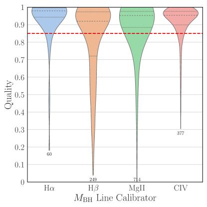
For broad lines used to estimate virial BH mass, we provide a $\chi_{\nu}^{2}$ statistic as well as a quality metric analogous to $R^{2}$ , which is used to asses how well the emission line model explains line flux variance that is not attributable to noise. Figure 6 shows violin plots of the distributions of the quality metric for each BH mass line calibrator. We consider a quality of 0.85 excellent for the use of calibration purposes for the relations derived in Sections 4.1, 4.2, and 4.3. Fits to broad H $\alpha$ are generally good, with 90% of cases with quality metrics $\geq 0.85$ . This is juxtaposed by a much lower number of fits with quality metrics $\geq 0.85$ for H $\beta$ , for which only 63% meet the criterion. Factors such as stellar continuum, Fe II contamination, and asymmetries that can be attributed to ionized gas outflows all contribute to the non-trivialities of fitting broad H $\beta$ , and we surmise that these factors play a role in a significantly lower fit quality. The fits to Mg II and C IV are comparatively better, with 80% and 86% of fits with quality metrics $\geq 0.85$ , respectively. This could be attributed to the fact that features in Regions 7 and 8, which contain Mg II and C IV, are generally more broad, and the continuum more featureless, allowing one to achieve a better quality fit by our metric, albeit with larger parameter uncertainties.

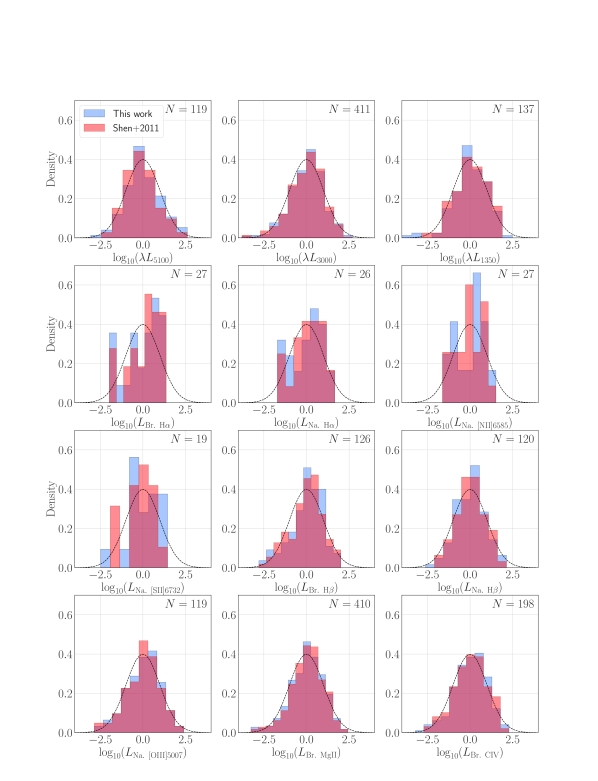
To validate our fitting results, we compare common fitted parameters against previously published catalogs of similar objects. The Shen et al. (2011) QSO catalog includes 38 parameters comparable to our catalog measurements for 506 broad line (QSO and Sy 1) objects in our sample (63%). Considering the differences in fitting models (e.g., line profile shapes, stellar/host continuum, multiple line components, etc.), we do expect some systematic offset in the distribution of parameter values. We report that the vast majority of systematic offsets in parameters between catalogs are significantly less than their respective scatter ( $<1\sigma$ on average), and once corrected for these offsets, more than 85% of variance between parameter distributions can be accounted for on average. Figure 7 shows the error-normalized distributions of select parameters between the two catalogs.

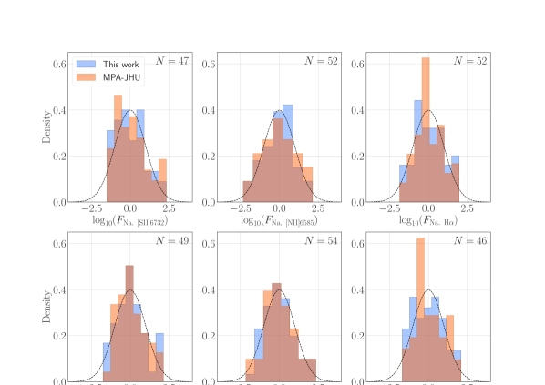
For the 92 objects in our catalog that are classified as Sy 2, we compare our parameter values to the SDSS DR8 MPA-JHU catalog of galaxy emission lines²²2http://www.mpa-garching.mpg.de/SDSS/, from which there are 55 object matches (60%) and 12 directly comparable parameters. We prefer the MPA-JHU catalog over the more-recent Portsmouth catalog (Thomas et al., 2013), although the general quality of the two catalogs similar in regards to emission line parameters. For Sy 2 types, we report that the systematic offsets between the MPA-JHU and our catalog is also significantly less than the scatter, and 91% of the variance in the parameter distributions is accounted for. A comparison of the error-normalized distributions of select parameters between our catalog and the MPA-JHU catalog is shown in Figure 8.

Given the excellent agreement between $\sim 63\%$ of our catalog with previously published catalogs, we conclude that our fitting method and results are sufficiently validated.

4 Derived Properties

Whereas the previous section detailed our method for fitting the continuum and line features of the ICRF3 objects, in this section we produce value-added properties derived from these fits. Our analysis includes quantities of relevance to virial BH mass estimation, including proxies of AGN luminosity, broad line width, and BH mass calibration between different estimators, and compare these to those in the literature.

4.1 AGN Luminosity

First, we investigate typical proxies of AGN luminosity, including those luminosities measured directly from the AGN component of the spectral continuum, as well as luminosities from the broad line profile of relevant estimators. Ideally, one would obtain an accurate estimate of the AGN luminosity from high-resolution imaging and performing surface-brightness decomposition of the AGN PSF from the host galaxy (Canalizo et al., 2012; Bentz & Manne-Nicholas, 2018; Sexton et al., 2019), and then use the $R_{\rm{BLR}}-L_{\rm{AGN}}$ relation from Bentz et al. (2013) to obtain a proxy for the broad line region size. However, a strong correlation between continuum and broad line luminosities and BH mass makes estimating AGN luminosity directly from single-epoch spectra a viable alternative, provided that the host stellar component of the continuum can be accurately subtracted from the AGN continuum component.

When possible, we prefer the continuum over the broad line luminosity, since the modelling of the continuum using the full spectrum is well-constrained, and not subject to uncertainties introduced by the shape of the broad line profile. Black hole masses estimated using the H $\alpha$ or H $\beta$ width estimator use the continuum luminosity at 5100Å, the Mg II width estimator uses the continuum luminosity at 3000Å, and C IV width estimator uses the continuum luminosity at 1350Å. When the continuum luminosity is not available for the respective broad line width estimator, we use the broad line luminosity as a proxy for the continuum luminosity to estimate BH mass.

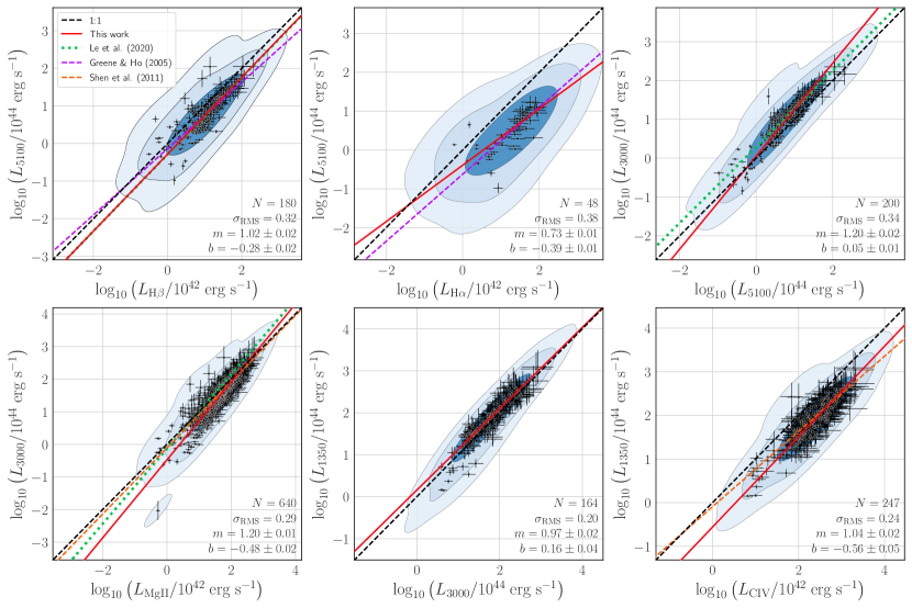
To verify that our measurements are valid proxies for AGN luminosity, we measure the log-linear relationship between various luminosity estimators and compare them to those found in the literature. We perform linear regression using maximum likelihood techniques, taking into account uncertainties in both variables, and estimate uncertainties in the slope and intercept using the affine-invariant Markov chain Monte Carlo (MCMC) sampler emcee (Foreman-Mackey et al., 2019). Figure 9 shows the kernel density estimation (KDE) distributions and fits to the various luminosity relations under consideration, as well as comparison fits from literature. The results of these fits are provided in Table 2.

In general, the intrinsic AGN continuum and broad emission line luminosities are strongly correlated, which is very important as BH virial mass estimation relies on accurate measurement of the intrinsic AGN continuum luminosity. Of these correlated luminosities, the relationship between H $\alpha$ and $\lambda L_{\rm{5100}}$ has the shallowest slope and greatest intrinsic RMS scatter; however, our relation agrees well with that of Greene & Ho (2005), which has a slope of 0.86. Relations with Mg II and C IV are also in good agreement with those from Shen et al. (2011) and Le et al. (2020).

From these relations, we can surmise that the relationships between broad line and continuum luminosities for exclusively radio-loud objects, such as those in the ICRF3 sample, appear to be statistically indistinguishable from the same relations for samples that may contain both radio-loud and/or radio-quiet objects. Previous studies (Boroson & Green, 1992; Brotherton, 1996) using correlation analysis and principal component analysis found significant differences between radio-loud and radio-quiet objects in equivalent widths of [O III], H $\beta$ , and Fe II, however continuum or broad line luminosities were not among these significant differences.

Table 2: Results of log-linear fits to various continuum and broad line luminosity relations, as shown in Figure 9.

Y	X	$m$	$b$	$\sigma_{\rm{RMS}}$
$\lambda L_{5100}$	$L_{\rm{H}\beta}$	$1.02\pm 0.02$	$-0.28\pm 0.02$	$0.32$
$\lambda L_{5100}$	$L_{\rm{H}\alpha}$	$0.73\pm 0.01$	$-0.39\pm 0.01$	$0.38$
$\lambda L_{3000}$	$\lambda L_{5100}$	$1.20\pm 0.02$	$0.05\pm 0.01$	$0.34$
$\lambda L_{3000}$	$\lambda L_{\rm{MgII}}$	$1.20\pm 0.01$	$-0.48\pm 0.02$	$0.29$
$\lambda L_{1350}$	$\lambda L_{3000}$	$0.97\pm 0.02$	$0.16\pm 0.04$	$0.20$
$\lambda L_{1350}$	$\lambda L_{\rm{CIV}}$	$1.04\pm 0.02$	$-0.56\pm 0.05$	$0.24$

Note. — Column 1: dependent variable. Column 2: independent variable. Column 3: best fit slope. Column 4: best fit $y$ -intercept. Column 5: Intrinsic RMS scatter (dex). Column 6: number of objects included in fit.

4.2 Broad Line Width

As with luminosity, we investigate the relations between width calibrators used in the calculation of BH mass to ensure the consistency and validity of our measurements. Figure 10 shows the various relationships between broad line width calibrators for dispersion and FWHM. Results of the fits to these relationships are provided in Table 3. We find that there is good agreement between different broad lines and their respective dispersions or FWHMs, on average.

We recover a comparable slope to Greene & Ho (2005) and Schlafly & Finkbeiner (2011) when comparing the FWHMs of H $\beta$ and H $\alpha$ , with the dispersions showing a similar slope, indicating that the ratio of the widths $\rm{FWHM}/\sigma$ converges to a constant value as expected by design of the symmetric line profile (pseudo-Voigt) chosen for this catalog.

When comparing the Mg II and H $\beta$ widths, we find a mean offset of $+0.13$ dex for $\sigma_{\rm{MgII}}$ relative to $\sigma_{\rm{H}\beta}$ , whereas the mean offset for FWHM is only $-0.03$ dex. We suspect that the excess dispersion relative to H $\beta$ is due to the fact that strong UV iron contamination in the wings of the line profile can bias the dispersion to larger values, and in part that Mg II is a doublet. Excess UV iron emission can push the pseudo-Voigt profile towards a Lorentzian shape with extended symmetric wings, biasing the dispersions toward higher values while leaving the FWHM unaffected. By comparison, the relation from Le et al. (2020) for both dispersion and FWHM have a negative offset by a comparable amount, while our offset for FWHM is closer to unity and more comparable to those of Shen et al. (2011). For Mg II, the difference in BH mass by choice of width estimator ( $\sigma$ versus FWHM) is 0.1 dex, with dispersion resulting in lower BH mass on average.

The C IV line profile is fit in a similar way to the Mg II profile, by considering the full line profile instead of decomposing the line into separate narrow and broad kinematic components. We fit a single broad pseudo-Voigt profile with a single narrow Gaussian profile. There appears to be a dichotomy of profile shapes for C IV, which differ by the presence of a peaked narrow component and thus requiring the single narrow Gaussian component in the model. We suspect that the difference in line profile shape is caused by truncation of the line profile due to narrow and broad metal absorption features typically observed in rest frame near-UV spectra. The C IV line is fit within Region 8, which is defined as $\lambda_{\rm{rest}}<2000$ Å, which is necessary to constrain an apparently weaker UV iron continuum, as well as other broad emission line features in the region.

We again observe a positive offset of 0.28 dex in dispersion when comparing C IV to Mg II, compared to an only 0.09 dex for FWHM, as shown in Figure 10. We suspect this is also caused by the biasing of the pseudo-Voigt line profile towards a Lorentzian shape, which increases the value of dispersion due to excess flux in the wings of the profile, despite the noise floor truncation we employ in the calculating of dispersion. It is uncertain if a multi-Gaussian (Shen et al., 2011) or Gauss-Hermite (Park et al., 2017) model would yield different results, since both implementations could allow for excess flux in the wings of the profile to be included in the model unless otherwise constrained. The difference in choice of width calibrator ( $\sigma$ versus FWHM) for the C IV is 0.17 dex, with dispersion resulting in a lower BH mass than FWHM on average.

Broad C IV is particularly difficult to obtain consistently reliable fits due to the prevalence of narrow and/or broad metal absorption features in the near-UV. We use an iterative moving median filter, which varies in size, to detect and interpolate over $3\sigma$ negative outliers. This method has a high success rate for narrow ( $<100$ km s^-1) features but fails to fully mask broader features ( $>1000$ km s^-1) which cover much larger portions of the fitting region. Shen et al. (2011) used a similar 20-pixel moving boxcar method to detect and mask absorption features at the $3\sigma$ level. We find that interpolation is preferable to masking, since the size of the mask is often such that a significant portion of the C IV line is masked, causing the fit to be unconstrained within the mask, whereas interpolation preserves these pixels as constraints for the fit. However, this method is only marginally better for cases in which large absorption features affect the C IV line profile, since we cannot fully reconstruct the original line shape from either method. The affect of strong absorption features on the C IV line profile can truncate the full amplitude of the line and bias the quantities derived from the model such as width, flux, and equivalent width. A larger study of the systematics regarding the fitting of C IV is necessary to address these modelling issues.

In summary, it would appear that when comparing across different line estimators (H $\alpha$ , H $\beta$ , Mg II, C IV), the FWHM width estimator is more consistent; that is, the FWHM measurements of different lines scale closer to unity. Lines such as Mg II and C IV, which can experience varying amounts of UV iron contamination, make choice of line profile shape non-trivial, and can lead to biased estimates in velocity dispersion. While dispersion has been considered the width estimator of choice for BH studies, in part due to the decreased scatter as shown in Figure 10, it is possible that FWHM may be a better and unbiased estimator of width across different line estimators. A systematic study of the relationship between line profile shapes across different line estimators is necessary to determine which model implementation is ideal for large samples.

Table 3: Results of log-linear fits to various broad line width relations, as shown in Figure 10.

Y	X	$m$	$b$	$\sigma_{\rm{RMS}}$
$\sigma_{\rm{H}\beta}$	$\sigma_{\rm{H}\alpha}$	$1.10\pm 0.01$	$-0.05\pm 0.01$	$0.15$
$\sigma_{\rm{MgII}}$	$\sigma_{\rm{H}\beta}$	$0.65\pm 0.01$	$0.18\pm 0.00$	$0.09$
$\sigma_{\rm{CIV}}$	$\sigma_{\rm{MgII}}$	$1.14\pm 0.02$	$0.21\pm 0.01$	$0.15$
$\rm{FWHM}_{\rm{H}\beta}$	$\rm{FWHM}_{\rm{H}\alpha}$	$0.89\pm 0.01$	$0.09\pm 0.01$	$0.19$
$\rm{FWHM}_{\rm{MgII}}$	$\rm{FWHM}_{\rm{H}\beta}$	$0.79\pm 0.01$	$0.11\pm 0.01$	$0.09$
$\rm{FWHM}_{\rm{CIV}}$	$\rm{FWHM}_{\rm{MgII}}$	$1.33\pm 0.03$	$0.14\pm 0.02$	$0.22$

4.3 Black Hole Mass

Estimates of BH mass are inferred from the size and kinematics of gas assumed to be virialized within the gravitational potential of the BH (Peterson, 2004), given by the equation

M_{\rm{BH}}=f\frac{\Delta V^{2}R_{\rm{BLR}}}{G}

(3)

where $f$ is the virial coefficient, $\Delta V$ is the gas velocity dispersion, $R_{\rm{BLR}}$ is the effective radius of the broad line region, and $G=5.124~{}\rm{km}^{2}~{}\rm{s}^{-2}~{}\rm{ld}~{}\rm{M}_{\odot}^{-1}$ is the gravitational constant in the relevant units. The virial coefficient $f$ is used to scale single-epoch BH estimates such that they are consistent with those of well-determined reverberation-mapped and quiescent galaxies using the broad H $\beta$ emission line. The gas velocity $\Delta V$ is estimated via the gas dispersion or FWHM of broad emission lines. The radius of the broad line region $R_{\rm{BLR}}$ is empirically determined from a strong correlation with the AGN luminosity at 5100 Å from Bentz et al. (2013), given by

	$\displaystyle\log_{10}\left(\frac{R_{\rm{BLR}}}{\rm{ld}}\right)$	$\displaystyle=(1.527\pm 0.031)+(0.533\pm 0.035)$
		$\displaystyle\times\log_{10}\left(\frac{\lambda L_{5100}}{10^{44}\rm{~{}erg~{}s}^{-1}}\right)$		(4)

Woo et al. (2015) determined the virial factor by re-calibrating the reverberation-mapped and quiescent galaxies, finding $\log_{10}(f)=0.05\pm 0.12$ and $\log_{10}(f)=0.65\pm 0.12$ for dispersion- and FWHM-based BH masses, respectively.

We use the above relations and values to determine BH mass for H $\beta$ line for both the dispersion and FWHM width estimators, and use H $\beta$ as the baseline for determining the appropriate calibration for H $\alpha$ and Mg II. We then use the Mg II BH mass to calibrate C IV BH masses.

The redshift range spanned by ICRF3 objects, as well as the available wavelength coverage in SDSS, ensures that the number and type of available broad lines and continuum luminosities required for single-epoch virial BH mass estimation varies from object to object. As a result, it is necessary to re-derive BH mass calibrators for Mg II and C IV in order to ensure that BH masses are self-consistent for all objects in the catalog. We note that while these calibrations have been performed in the literature in the past, calibrations of these estimators have not been performed for a sample of exclusively radio-loud objects.

The functional form of the BH mass estimator we adopt is given by

	$\displaystyle\log_{10}\left(\frac{M_{\rm{BH}}}{\rm{M}_{\odot}}\right)=~{}$	$\displaystyle\alpha+\beta\log_{10}\left(\frac{\Delta V}{10^{3}\rm{\;km\;s}^{-1}}\right)$		(5)
		$\displaystyle+\gamma\log_{10}\left(\frac{\lambda L_{\lambda}}{10^{44}\rm{\;erg\;s}^{-1}}\right)$		(6)

where $\Delta V$ is estimated using either the broad line dispersion ( $\sigma$ ) or FWHM, and $\lambda L_{\lambda}$ is the monochromatic luminosity of the AGN measured from the AGN continuum (power-law component) of the best-fit model. The coefficients $\beta=2.0$ and $\gamma=0.5$ were fixed constants in the calculation of $\alpha$ for both the H $\alpha$ , Mg II, and C IV calibrations.

If instead the integrated luminosity of the broad line is used to as a proxy for the monochromatic AGN luminosity, the functional form of the BH mass estimator used to estimate $\alpha$ becomes:

	$\displaystyle\log_{10}\left(\frac{M_{\rm{BH}}}{\rm{M}_{\odot}}\right)=~{}$	$\displaystyle\alpha+\beta\log_{10}\left(\frac{\Delta V}{10^{3}\rm{\;km\;s}^{-1}}\right)+$
		$\displaystyle\gamma\log_{10}\left(\frac{L_{\rm{br.}}}{10^{42}\rm{\;erg\;s}^{-1}}\right)$		(7)

where $L_{\rm{br.}}$ is the integrated broad line luminosity, and the luminosity scaling factor becomes $10^{42}$ erg s^-1, following the conventions frequently used in the literature. We calibrate H $\alpha$ and Mg II BH masses using H $\beta$ BH masses to determine the best fitting $\alpha$ . Due to the wavelength range of the SDSS, we cannot use H $\beta$ to determine the calibration for C IV, and therefore Mg II is used for the calibration of C IV instead, with uncertainties for these calibrations propagated appropriately.

The results of the calibrations for H $\alpha$ , Mg II, and C IV are provided in Table 4. Objects used for calibrations are those with line detections of at least 95% and quality flags of at least 0.85 to ensure that poor quality fits do not adversely bias the calibration. The dispersion width calibrator consistently results in the lowest scatter in each resulting calibration, while the FWHM width calibrator consistently produces the most amount of scatter. The scatter is largest at $\sim 0.36$ dex for the C IV, likely due to increased scatter in both FWHM and dispersion, combined with the stronger dependence on width in Equations 6 and 7. The resulting values of $\alpha$ in Table 4 are used to calculate BH mass for H $\alpha$ , Mg II, and C IV.

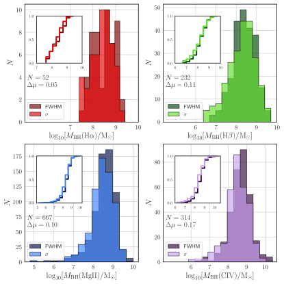
Considering the availability of the four broad line BH estimators for each spectrum, there are a total of 795 objects with unique BH masses, of which 467 (59%) have at least two estimates of BH mass from available broad lines. The BH mass distributions for H $\alpha$ , H $\beta$ , Mg II, and C IV calibrators, for both dispersion and FWHM-based BH mass, are shown in Figure 11. Average uncertainty for H $\beta$ masses derived from empirical relations is 0.46 dex, based on the scatter derived from the calibration of the virial factor from Woo et al. (2015) as well as uncertainties in the measurements of width and luminosity. Average uncertainties for H $\alpha$ , Mg II, and C IV are $\sim 0.51$ dex for dispersion and $\sim 0.55$ for FWHM.

We find that dispersion systematically overestimates BH mass relative to masses estimated using FWHM, with the largest differences found in C IV, with a mean offset of $+0.17$ dex. The H $\beta$ and Mg II BH masses show nearly identical mean offsets at $+0.11$ dex, and H $\alpha$ shows the least difference at $+0.05$ dex. We suspect that the difference in BH mass estimated with dispersion is due to the bias towards a Lorentzian profile of our pseudo-Voigt implementation, caused by optical Fe II and UV iron emission in the regions including H $\beta$ , Mg II, and C IV. Optical Fe II emission generally extends up to 7000Å; however, the relative intensities of Fe II for our model (Véron-Cetty et al., 2004) are significantly weaker than they are near H $\beta$ .

Table 4: Calibration of H

\alpha

, Mg II, and C IV BH mass for the ICRF3 sample.

$\Delta V$	$L_{\lambda}$	$\alpha$	$\mu_{\rm{offset}}$	$\sigma_{\rm{RMS}}$
			(dex)	(dex)
$\sigma_{\rm{H}\alpha}$	$\lambda L_{\rm{5100}}$	$7.46\pm 0.07$	$0.00$	$0.25$
$\sigma_{\rm{H}\alpha}$	$L_{\rm{H}\alpha}$	$7.06\pm 0.07$	$+0.03$	$0.26$
$\rm{FWHM}_{\rm{H}\alpha}$	$\lambda L_{\rm{5100}}$	$6.91\pm 0.07$	$-0.03$	$0.31$
$\rm{FWHM}_{\rm{H}\alpha}$	$L_{\rm{H}\alpha}$	$6.50\pm 0.07$	$-0.06$	$0.31$
$\sigma_{\rm{MgII}}$	$\lambda L_{\rm{3000}}$	$7.20\pm 0.04$	$-0.03$	$0.27$
$\sigma_{\rm{MgII}}$	$L_{\rm{MgII}}$	$7.07\pm 0.04$	$-0.01$	$0.32$
$\rm{FWHM}_{\rm{MgII}}$	$\lambda L_{\rm{3000}}$	$6.83\pm 0.04$	$+0.01$	$0.32$
$\rm{FWHM}_{\rm{MgII}}$	$L_{\rm{MgII}}$	$6.69\pm 0.04$	$-0.02$	$0.36$
$\sigma_{\rm{CIV}}$	$\lambda L_{\rm{1350}}$	$6.60\pm 0.06$	$-0.03$	$0.26$
$\sigma_{\rm{CIV}}$	$L_{\rm{CIV}}$	$6.39\pm 0.06$	$-0.03$	$0.30$
$\rm{FWHM}_{\rm{CIV}}$	$\lambda L_{\rm{1350}}$	$6.63\pm 0.06$	$-0.13$	$0.36$
$\rm{FWHM}_{\rm{CIV}}$	$L_{\rm{CIV}}$	$6.42\pm 0.06$	$-0.16$	$0.35$

Note. — Column 1: velocity calibrator. Column 2: luminosity calibrator. Column 3: best-fit $\alpha$ . Column 4: mean offset of residuals from unity. Column 5: Intrinsic RMS scatter.

5 General Properties of ICRF3 Objects

5.1 AGN Spectral Type

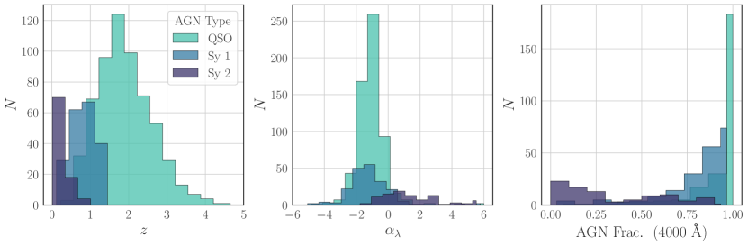
We classify each ICRF3 object in our sample by its AGN spectral type, of which there are four that can be distinguished by general spectroscopic characteristics. These four AGN spectral types are “QSO”, “Sy 1”, “Sy 2”, and “featureless”, and are provided in the catalog for each object by the “AGN_TYPE” column.

The vast majority ( $N=602$ ) of ICRF3 objects are quasars (QSOs), which are typically at the highest redshifts in the sample. Quasars are typically distinguished by their luminosities, which are comparatively higher than those of Sy 1 objects. The AGN power-law continuum, parameterized by index $\alpha_{\lambda}$ , is nearly identical between Sy 1 objects and QSOs; QSOs in our sample have a mean $\alpha_{\lambda}=-1.58$ , while Sy 1 objects have a mean $\alpha_{\lambda}=-1.56$ . To further distinguish these two classes, we consider the fraction of the total continuum at 4000Å attributed solely to the AGN continuum. For our sample, we classify an object as a QSO if the continuum fraction at 4000 Å is consistent with unity, within its $1\sigma$ uncertainty, that is, there is no detectable host galaxy component in the spectrum at 4000 Å. The distributions of QSOs with redshift, $\alpha_{\lambda}$ , and AGN flux fraction at 4000 Å is shown in Figure 12.

Sy 1 objects ( $N=198$ ) occupy an intermediate space in redshift between QSOs and type 2 objects, and are therefore distinguished by a strong AGN fraction at 4000Å and strong host galaxy fractions at 7000Å. The majority of Sy 1 objects have AGN continuum fractions at 4000Å greater than 50%.

Finally, Sy 2 objects ( $N=92$ ), which have host galaxy contributions that dominate the entire optical spectrum, presumably due to obscuration of the AGN, occupy the lowest redshifts in the ICRF3 sample. The shape of the AGN power-law continuum for Sy 2 objects is closer to flat with a mean $\alpha_{\lambda}=1.01$ . The AGN fraction at 4000Å is negligible or is is consistent with zero, and the lack of dilution from an AGN continuum coupled with lower redshifts can allow for accurate recovery of the stellar LOSVD due to higher S/N.

A fourth class of 122 objects, for which the only spectral feature is a featureless power-law continuum, we classify as “featureless” in the catalog. The lack of any spectral features, coupled with the fact that these are radio-loud objects, may indicate that these are AGNs with featureless radio continua beamed into the LOS. Because they have no distinguishing emission or absorption line features, we cannot determine the redshifts of these objects. We do however provide values and uncertainties for the power-law continuum slope for these objects to characterize the general shape of the spectrum.

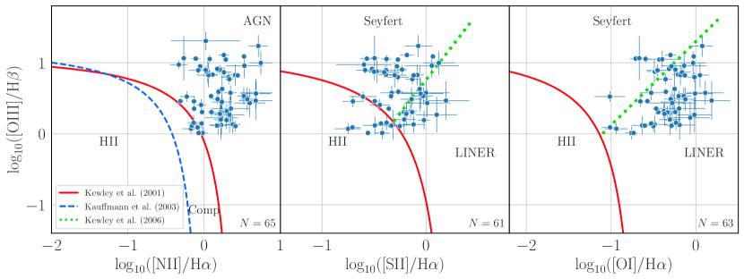
5.2 BPT Diagrams of Type 2 Objects

While we have assumed that accretion onto a SMBH is the primary engine powering radio-loud emission in ICRF3 objects, it is not obvious from the spectra of Sy 2 objects that this is the case, due to a lack of distinguishing AGN features such as broad lines or a steep power-law continuum. We can further classify Sy 2 objects in our sample using BPT diagrams (Baldwin et al., 1981) to determine if other radiative mechanisms contribute to the optical emission we observe.

Figure 13 shows the three BPT diagrams for objects classified as Sy 2 in our sample. The H $\alpha$ BPT diagram (left panel of Figure 13) classifies the majority of our objects as AGNs, with only a handful of objects in the composite category and none in the star-forming H II region category. The [S II] and [O I] BPT diagrams (middle and right panels of Figure 13, respectively) show slightly differing distributions, with a handful of objects classified as H II or low-ionization nuclear emission-line region (LINER) types for [S II], and the majority as LINER for [O I]. However, given the relative strengths of [S II] and [O I] compared to H $\alpha$ , these BPT classifications are likely less reliable compared to the H $\alpha$ BPT diagram. Nevertheless, all three BPT diagrams show clear preference toward larger flux ratios inconsistent with H II regions. We therefore conclude that the Sy 2 classified objects within our sample are likely obscured AGNs.

Finally, while it is possible that the emission from type 1 objects may not be completely dominated by the emission from the AGN, as in the case of Sy 1 types, we do not attempt to classify Sy 1 or QSOs based on BPT classification, as the presence of broad line emission can result in poor constraints on the fitting of narrow H $\alpha$ and H $\beta$ , resulting in large uncertainties in line ratios and/or questionable results.

5.3 BH Mass & Accretion Rate

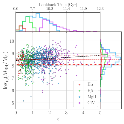
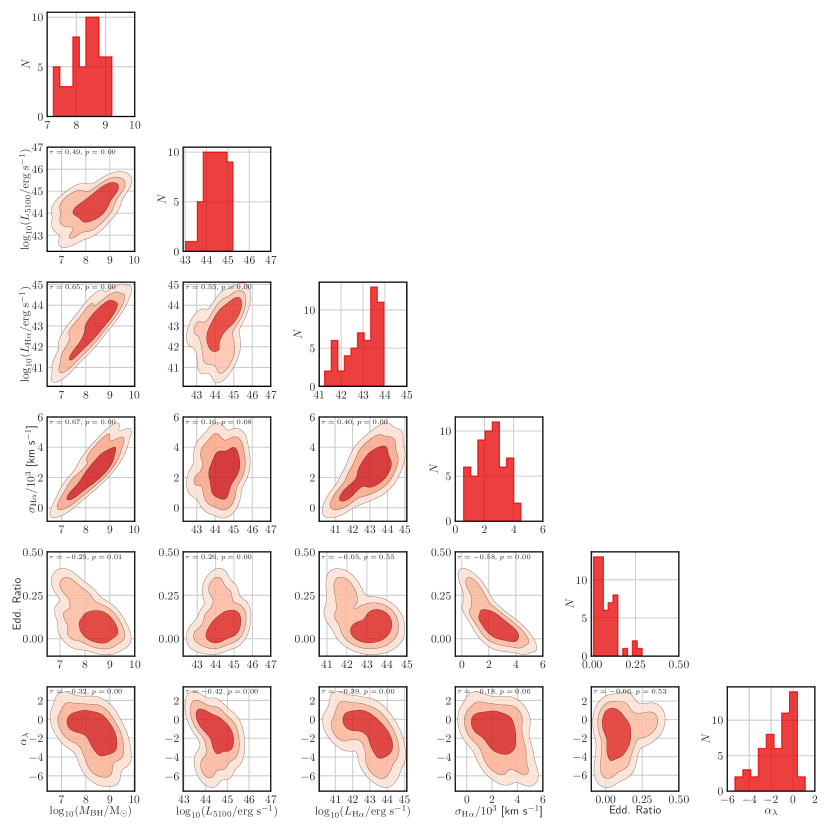
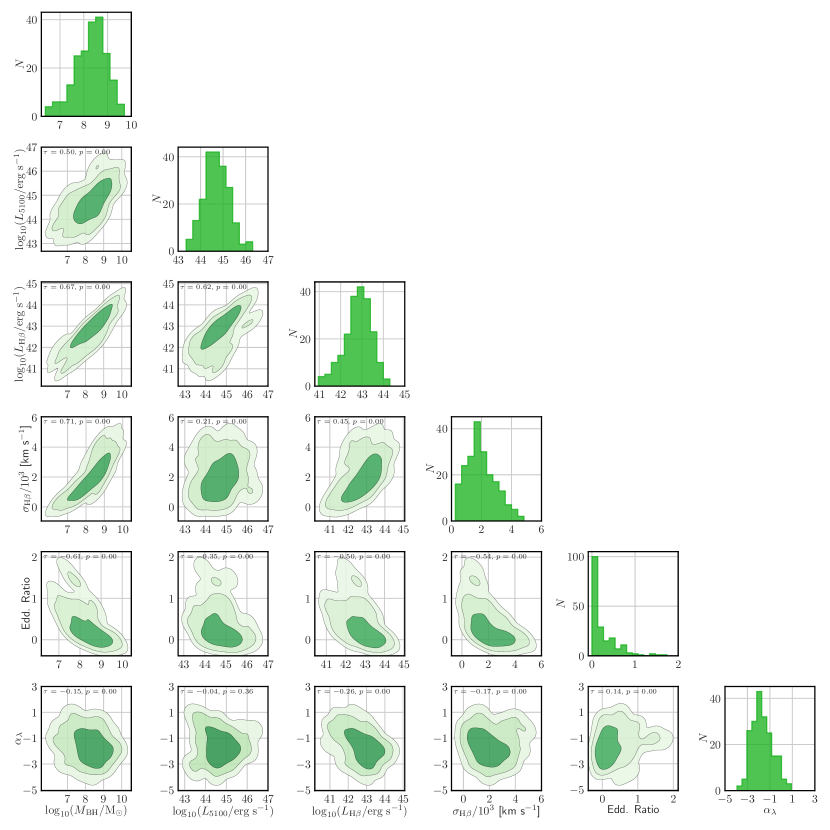
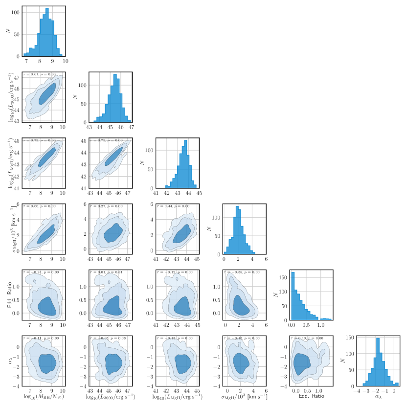
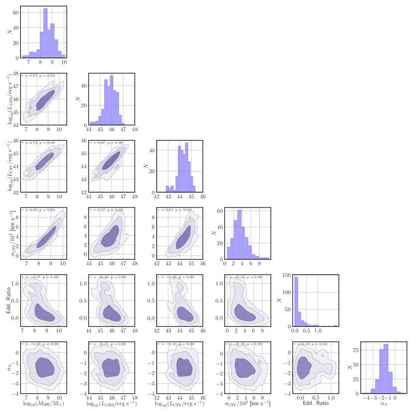
We plot the distribution of BH mass for all line calibrators as a function of cosmic time in Figure 14. The BH masses as a function of $z$ have a slope of $0.08\pm 0.03$ , significant at the $2.7\sigma$ level. The relation is dominated by a total scatter of $\sigma_{\rm{RMS}}=0.68$ dex and and intrinsic scatter of $\sigma_{\rm{intr}}=0.30$ dex. Despite the fact that our objects are radio selected, the number of spectra from which we can accurately measure BH mass is greatest for those at $z>1$ , and we are likely sampling from the highest-luminosity– and therefore highest-mass –objects in the BH mass distribution at high $z$ (Lauer et al., 2007; Shen et al., 2008). Notwithstanding any effects of optical selection bias, the distribution of BH masses at all $z$ is generally flat over the last 12.3 Gyr, with a median value of $8.48$ in $\log_{10}(M_{\rm{BH}}/\rm{M}_{\odot})$ and median absolute deviation of $0.38$ dex. The median BH mass range for the ICRF3 sample agrees with other studies that have found that BH masses in radio-loud AGNs are typically more massive than those in radio-quiet AGNs (Franceschini et al., 1998; McLure et al., 1999; McLure & Dunlop, 2000). Similar studies of radio-loud quasars have found strong anti-correlations between radio loudness and BH mass, showing that a majority of radio-loud quasars have $M_{\rm{BH}}>10^{8}~{}\rm{M}_{\odot}$ (Laor, 2000; Gu et al., 2001), while other studies have found that radio-loud quasars have a larger distribution of BH mass (Ho, 2002). Our results appear to agree with the latter claim that BH mass can have a broad distribution across a wide range of redshifts regardless of estimator used, but we have made no attempt to correct for the effect of optical selection bias. A comprehensive study on the differences between radio-loud and radio-quiet objects with larger statistical samples that control for BH mass are needed to disentangle the apparent anti-correlation between BH mass and radio-loudness, but this is beyond the scope of this work.

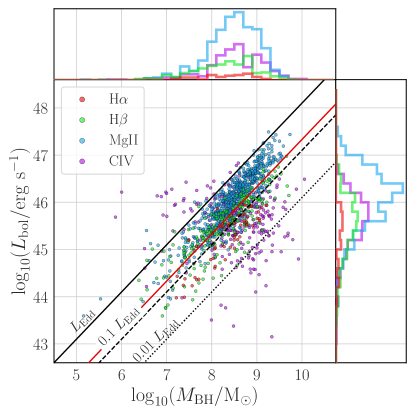
In Figure 15 we plot bolometric luminosities as a function of BH mass to assess the distribution of Eddington radio for the ICRF3 sample. Bolometric luminosities are estimated using the relations derived by Runnoe et al. (2012a, b), who found that the monochromatic bolometric corrections between radio-loud and radio-quiet objects are consistent with 95% confidence. Instead of using luminosities measured directly from the spectral continuum, we use emission line luminosities following Wu et al. (2004), who suggested that the presence of strong optical jets in radio-loud quasars can significantly boost apparent AGN luminosity as estimated from the optical continuum. The luminosity of the broad line emission used to estimate BH mass may be a more direct estimate of the intrinsic AGN accretion luminosity than that measured from the continuum, the latter of which has contributions from many components (e.g, Fe II, UV iron, Balmer pseudo-continuum, jet emission, and stellar emission). Indeed, we observe slightly larger scatter in bolometric luminosities when using the optical continuum luminosities, and there is a tighter correlation observed between $M_{\rm{BH}}$ and line luminosities (also see Figures 16 - 19) than with continuum luminosities. We note, however, that estimates of $M_{\rm{BH}}$ have a greater dependence on line width than continuum luminosity, and the line widths and line luminosities are strongly correlated.

We find a similar result to Shen (2013), which is a general stratification of Eddington ratio with line calibrator, likely due to luminosity-dependent selection effects with increased redshift. The H $\alpha$ line calibrator typically provides the lowest Eddington ratios at $\sim 0.1~{}L_{\rm{Edd}}$ , and rises toward $L_{\rm{Edd}}$ in sequence with H $\beta$ , Mg II, and C IV. The median accretion rate for the entire sample is $\sim 17\%$ , however with considerable scatter. The C IV line shows the greatest scatter, likely due to the fitting peculiarities mentioned in Section 4.2. We note that estimates of bolometric luminosity have considerable uncertainties, and that these first-order monochromatic bolometric corrections should be used with caution. A complete modelling of the full spectral energy distribution for ICRF3 targets is necessary to acquire more accurate estimates of the bolometric luminosity and accretion rate, which we will perform in a future study.

In Figures 16 - 19 we plot the covariance matrices for all BH mass estimators and relevant parameters. Among the strongest of these correlations with BH mass are continuum luminosity, line luminosity, line width, and Eddington ratio, with Kendall’s $\tau\sim 0.5$ across all estimators. Other correlations, such as those with power-law slope $\alpha_{\lambda}$ , are significantly weaker.

6 Catalog Structure

We summarize the structure of the catalog. There exist two version of the USNO VLBI Spectroscopic Catalog: (1) a shorter form that provides all parameters and derived quantities pertaining to BH masses, BPT diagrams, luminosities, Eddington ratios, and lines listed in boldface in Table 5, and (2) a longer form that includes all quantities included in the shorter table with additional parameters for all emission lines. Individual column numbers, names, data types, and descriptions for the short table are given in Table 6.

There are a few caveats of note when using this catalog:

1.

The cosmology adopted for this work ( $H_{0}=70$ km s^-1 Mpc^-1, $\Omega_{\mathrm{m}}=0.3$ ) is used for reported continuum and emission line luminosities, and hence affects derived values of $M_{\rm{BH}}$ , bolometric luminosities, and Eddington ratios.
2.

Uncertainties for BH mass include uncertainties from width and luminosity estimators, as well as uncertainties derived from their respective calibrations. Since all BH mass calibrations rely on reverberation-mapped and dynamical masses derived using H $\beta$ , the minimum uncertainty on all reported BH masses is 0.44 dex.
3.

Quantities such as bolometric luminosity and Eddington ratio have significant uncertainties that can be attributed to the uncertainties attributed to using monochromatic bolometric corrections as opposed to modeling the full spectral energy distribution, so should be used with caution.
4.

Stellar kinematics, while reported for all objects whose ranges coincide with the Ca K+H, Mg Ib, and Ca T regions, should only be trusted for Sy 2 objects for which there is little to no AGN dilution of the continuum. These objects can be queried using the AGN_TYPE column.
5.

Caution should be taken when using lines with best-fit parameters close to the hard limits imposed on the fits (Section 3.4).

7 Summary

We have produced the first dedicated catalog of emission line properties of ICRF3 objects, such as emission line fluxes, stellar kinematics, AGN spectral types, and black hole masses. This catalog will aid in building a more complete physical understanding of the radio-loud AGNs that comprise the ICRF, aiding in the further development and refinement of the celestial reference frame.

Development and refinement of the ICRF is a continuous and indefinite process, and outstanding issues exist with the effort to make the ICRF wavelength-independent, such as the presence of discrepancies between the optical (i.e., Gaia) and radio VLBI source positions. These issues are likely to be in large part astrophysical in nature, motivating efforts to physically characterize the objects that comprise the ICRF. Reliable spectroscopic redshifts, radio loudness, jet orientation angle, and perhaps even the relative accretion rate may prove to be important considerations in source selection and weighting for a multi-wavelength ICRF. This catalog provides an important reference for such work.

In producing this catalog, we have additionally derived black hole virial mass scaling relations using C IV, Mg II, and H $\beta$ that are self-consistent, which will be useful to studies of radio-loud AGNs that span a large range in redshifts.

This catalog was produced using state-of-the-art Bayesian spectral fitting code that simultaneously fits all spectral parameters and performs posterior sampling using Markov chains. This code is, written in Python, has been updated since the last release (Sexton et al., 2021) to handle moderate-to-high redshift AGNs, and is a powerful tool for the AGN community.³³3https://github.com/remingtonsexton/BADASS3

Finally, we note that this will be a living catalog, with updates and additions to occur as archival data from other facilities is incorporated and new data becomes available. Where available, data spanning multiple epochs will be analyzed and time domain behavior noted. These updates and additions will be announced in brief publications or research notes.

We thank Valeri Makarov and Jeffery Munn for their helpful and insightful comments in the review of this catalog and manuscript. This research was funded primarily by USNO to support its ongoing research into reference frame objects. This research made use of Astropy,⁴⁴4http://www.astropy.org

a community-developed core Python package for Astronomy (Astropy Collaboration et al., 2013, 2018), as well as topcat (Taylor, 2005). Funding for the Sloan Digital Sky Survey IV has been provided by the Alfred P. Sloan Foundation, the U.S. Department of Energy Office of Science, and the Participating Institutions. SDSS acknowledges support and resources from the Center for High-Performance Computing at the University of Utah. The SDSS web site is www.sdss.org. SDSS is managed by the Astrophysical Research Consortium for the Participating Institutions of the SDSS Collaboration including the Brazilian Participation Group, the Carnegie Institution for Science, Carnegie Mellon University, Center for Astrophysics — Harvard & Smithsonian (CfA), the Chilean Participation Group, the French Participation Group, Instituto de Astrofísica de Canarias, The Johns Hopkins University, Kavli Institute for the Physics and Mathematics of the Universe (IPMU) / University of Tokyo, the Korean Participation Group, Lawrence Berkeley National Laboratory, Leibniz Institut für Astrophysik Potsdam (AIP), Max-Planck-Institut für Astronomie (MPIA Heidelberg), Max-Planck-Institut für Astrophysik (MPA Garching), Max-Planck-Institut für Extraterrestrische Physik (MPE), National Astronomical Observatories of China, New Mexico State University, New York University, University of Notre Dame, Observatório Nacional / MCTI, The Ohio State University, Pennsylvania State University, Shanghai Astronomical Observatory, United Kingdom Participation Group, Universidad Nacional Autónoma de México, University of Arizona, University of Colorado Boulder, University of Oxford, University of Portsmouth, University of Utah, University of Virginia, University of Washington, University of Wisconsin, Vanderbilt University, and Yale University.

References

Arias et al. (1995) Arias, E. F., Charlot, P., Feissel, M., & Lestrade, J. F. 1995, A&A, 303, 604
Assafin et al. (2013) Assafin, M., Vieira-Martins, R., Andrei, A. H., Camargo, J. I. B., & da Silva Neto, D. N. 2013, MNRAS, 430, 2797, doi: 10.1093/mnras/stt081
Astropy Collaboration et al. (2013) Astropy Collaboration, Robitaille, T. P., Tollerud, E. J., et al. 2013, A&A, 558, A33, doi: 10.1051/0004-6361/201322068
Astropy Collaboration et al. (2018) Astropy Collaboration, Price-Whelan, A. M., Sipőcz, B. M., et al. 2018, AJ, 156, 123, doi: 10.3847/1538-3881/aabc4f
Baldwin et al. (1981) Baldwin, J. A., Phillips, M. M., & Terlevich, R. 1981, PASP, 93, 5, doi: 10.1086/130766
Bentz & Manne-Nicholas (2018) Bentz, M. C., & Manne-Nicholas, E. 2018, ApJ, 864, 146, doi: 10.3847/1538-4357/aad808
Bentz et al. (2013) Bentz, M. C., Denney, K. D., Grier, C. J., et al. 2013, ApJ, 767, 149, doi: 10.1088/0004-637X/767/2/149
Berton et al. (2020) Berton, M., Järvelä, E., Crepaldi, L., et al. 2020, A&A, 636, A64, doi: 10.1051/0004-6361/202037793
Blandford et al. (2019) Blandford, R., Meier, D., & Readhead, A. 2019, ARA&A, 57, 467, doi: 10.1146/annurev-astro-081817-051948
Blanton et al. (2017) Blanton, M. R., Bershady, M. A., Abolfathi, B., et al. 2017, AJ, 154, 28, doi: 10.3847/1538-3881/aa7567
Boroson & Green (1992) Boroson, T. A., & Green, R. F. 1992, ApJS, 80, 109, doi: 10.1086/191661
Brotherton (1996) Brotherton, M. S. 1996, ApJS, 102, 1, doi: 10.1086/192249
Calderone et al. (2017) Calderone, G., Nicastro, L., Ghisellini, G., et al. 2017, MNRAS, 472, 4051, doi: 10.1093/mnras/stx2239
Canalizo et al. (2012) Canalizo, G., Wold, M., Hiner, K. D., et al. 2012, ApJ, 760, 38, doi: 10.1088/0004-637X/760/1/38
Cappellari (2017) Cappellari, M. 2017, MNRAS, 466, 798, doi: 10.1093/mnras/stw3020
Cardelli et al. (1989) Cardelli, J. A., Clayton, G. C., & Mathis, J. S. 1989, ApJ, 345, 245, doi: 10.1086/167900
Charlot et al. (2020) Charlot, P., Jacobs, C. S., Gordon, D., et al. 2020, A&A, 644, A159, doi: 10.1051/0004-6361/202038368
da Silva Neto et al. (2002) da Silva Neto, D. N., Andrei, A. H., Vieira Martins, R., & Assafin, M. 2002, AJ, 124, 612, doi: 10.1086/341163
Dawson et al. (2013) Dawson, K. S., Schlegel, D. J., Ahn, C. P., et al. 2013, AJ, 145, 10, doi: 10.1088/0004-6256/145/1/10
Dawson et al. (2016) Dawson, K. S., Kneib, J.-P., Percival, W. J., et al. 2016, AJ, 151, 44, doi: 10.3847/0004-6256/151/2/44
Dietrich et al. (2002) Dietrich, M., Appenzeller, I., Vestergaard, M., & Wagner, S. J. 2002, ApJ, 564, 581, doi: 10.1086/324337
Dorland et al. (2020) Dorland, B., Secrest, N., Johnson, M., et al. 2020, in Astrometry, Earth Rotation, and Reference Systems in the GAIA era, ed. C. Bizouard, 165–171. https://arxiv.org/abs/2009.02169
Eisenstein et al. (2011) Eisenstein, D. J., Weinberg, D. H., Agol, E., et al. 2011, AJ, 142, 72, doi: 10.1088/0004-6256/142/3/72
Fernandez et al. (2022) Fernandez, L. C., Secrest, N. J., Johnson, M. C., et al. 2022, arXiv e-prints, arXiv:2201.05152. https://arxiv.org/abs/2201.05152
Fey et al. (2015) Fey, A. L., Gordon, D., Jacobs, C. S., et al. 2015, AJ, 150, 58, doi: 10.1088/0004-6256/150/2/58
Fischer et al. (2021) Fischer, T. C., Secrest, N. J., Johnson, M. C., et al. 2021, ApJ, 906, 88, doi: 10.3847/1538-4357/abca3c
Foreman-Mackey et al. (2019) Foreman-Mackey, D., Farr, W., Sinha, M., et al. 2019, The Journal of Open Source Software, 4, 1864, doi: 10.21105/joss.01864
Franceschini et al. (1998) Franceschini, A., Vercellone, S., & Fabian, A. C. 1998, MNRAS, 297, 817, doi: 10.1046/j.1365-8711.1998.01534.x
Fricke et al. (1988) Fricke, W., Schwan, H., Lederle, T., et al. 1988, Veroeffentlichungen des Astronomischen Rechen-Instituts Heidelberg, 32, 1
Grandi (1982) Grandi, S. A. 1982, ApJ, 255, 25, doi: 10.1086/159799
Greene & Ho (2005) Greene, J. E., & Ho, L. C. 2005, ApJ, 630, 122, doi: 10.1086/431897
Greene & Ho (2006) —. 2006, ApJ, 641, 117, doi: 10.1086/500353
Gu et al. (2001) Gu, M., Cao, X., & Jiang, D. R. 2001, MNRAS, 327, 1111, doi: 10.1046/j.1365-8711.2001.04795.x
Heckman (1980) Heckman, T. M. 1980, A&A, 500, 187
Ho (2002) Ho, L. C. 2002, ApJ, 564, 120, doi: 10.1086/324399
Kauffmann et al. (2003) Kauffmann, G., Heckman, T. M., Tremonti, C., et al. 2003, MNRAS, 346, 1055, doi: 10.1111/j.1365-2966.2003.07154.x
Kewley et al. (2001) Kewley, L. J., Dopita, M. A., Sutherland, R. S., Heisler, C. A., & Trevena, J. 2001, ApJ, 556, 121, doi: 10.1086/321545
Kewley et al. (2006) Kewley, L. J., Groves, B., Kauffmann, G., & Heckman, T. 2006, MNRAS, 372, 961, doi: 10.1111/j.1365-2966.2006.10859.x
Kovalev et al. (2017) Kovalev, Y. Y., Petrov, L., & Plavin, A. V. 2017, A&A, 598, L1, doi: 10.1051/0004-6361/201630031
Laor (2000) Laor, A. 2000, ApJ, 543, L111, doi: 10.1086/317280
Lauer et al. (2007) Lauer, T. R., Tremaine, S., Richstone, D., & Faber, S. M. 2007, ApJ, 670, 249, doi: 10.1086/522083
Le et al. (2020) Le, H. A. N., Woo, J.-H., & Xue, Y. 2020, ApJ, 901, 35, doi: 10.3847/1538-4357/abada0
Leighly (1999) Leighly, K. M. 1999, ApJS, 125, 297, doi: 10.1086/313277
Ma et al. (1998) Ma, C., Arias, E. F., Eubanks, T. M., et al. 1998, AJ, 116, 516, doi: 10.1086/300408
Makarov et al. (2019) Makarov, V. V., Berghea, C. T., Frouard, J., Fey, A., & Schmitt, H. R. 2019, ApJ, 873, 132, doi: 10.3847/1538-4357/aafa1c
Malkin (2018) Malkin, Z. 2018, ApJS, 239, 20, doi: 10.3847/1538-4365/aae777
McLure & Dunlop (2000) McLure, R. J., & Dunlop, J. S. 2000, MNRAS, 317, 249, doi: 10.1046/j.1365-8711.2000.03509.x
McLure et al. (1999) McLure, R. J., Kukula, M. J., Dunlop, J. S., et al. 1999, MNRAS, 308, 377, doi: 10.1046/j.1365-8711.1999.02676.x
Mignard et al. (2016) Mignard, F., Klioner, S., Lindegren, L., et al. 2016, A&A, 595, A5, doi: 10.1051/0004-6361/201629534
Napier et al. (1994) Napier, P. J., Bagri, D. S., Clark, B. G., et al. 1994, IEEE Proceedings, 82, 658, doi: 10.1109/5.284733
Nelson & Whittle (1996) Nelson, C. H., & Whittle, M. 1996, ApJ, 465, 96, doi: 10.1086/177405
Orosz & Frey (2013) Orosz, G., & Frey, S. 2013, A&A, 553, A13, doi: 10.1051/0004-6361/201321279
Park et al. (2017) Park, D., Barth, A. J., Woo, J.-H., et al. 2017, ApJ, 839, 93, doi: 10.3847/1538-4357/aa6a53
Peterson (2004) Peterson, B. M. 2004, in The Interplay Among Black Holes, Stars and ISM in Galactic Nuclei, ed. T. Storchi-Bergmann, L. C. Ho, & H. R. Schmitt, Vol. 222, 15–20, doi: 10.1017/S1743921304001358
Petrov & Kovalev (2017) Petrov, L., & Kovalev, Y. Y. 2017, MNRAS, 467, L71, doi: 10.1093/mnrasl/slx001
Petrov et al. (2019) Petrov, L., Kovalev, Y. Y., & Plavin, A. V. 2019, MNRAS, 482, 3023, doi: 10.1093/mnras/sty2807
Plavin et al. (2019) Plavin, A. V., Kovalev, Y. Y., Pushkarev, A. B., & Lobanov, A. P. 2019, MNRAS, 485, 1822, doi: 10.1093/mnras/stz504
Runnoe et al. (2012a) Runnoe, J. C., Brotherton, M. S., & Shang, Z. 2012a, MNRAS, 422, 478, doi: 10.1111/j.1365-2966.2012.20620.x
Runnoe et al. (2012b) —. 2012b, MNRAS, 427, 1800, doi: 10.1111/j.1365-2966.2012.21878.x
Schlafly & Finkbeiner (2011) Schlafly, E. F., & Finkbeiner, D. P. 2011, ApJ, 737, 103, doi: 10.1088/0004-637X/737/2/103
Sexton et al. (2019) Sexton, R. O., Canalizo, G., Hiner, K. D., et al. 2019, ApJ, 878, 101, doi: 10.3847/1538-4357/ab21d5
Sexton et al. (2021) Sexton, R. O., Matzko, W., Darden, N., Canalizo, G., & Gorjian, V. 2021, MNRAS, 500, 2871, doi: 10.1093/mnras/staa3278
Shen (2013) Shen, Y. 2013, Bulletin of the Astronomical Society of India, 41, 61. https://arxiv.org/abs/1302.2643
Shen et al. (2008) Shen, Y., Greene, J. E., Strauss, M. A., Richards, G. T., & Schneider, D. P. 2008, ApJ, 680, 169, doi: 10.1086/587475
Shen et al. (2011) Shen, Y., Richards, G. T., Strauss, M. A., et al. 2011, ApJS, 194, 45, doi: 10.1088/0067-0049/194/2/45
Sulentic (1989) Sulentic, J. W. 1989, ApJ, 343, 54, doi: 10.1086/167684
Taylor (2005) Taylor, M. B. 2005, Astronomical Society of the Pacific Conference Series, Vol. 347, TOPCAT & STIL: Starlink Table/VOTable Processing Software (Astronomical Society of the Pacific), 29
Thomas et al. (2013) Thomas, D., Steele, O., Maraston, C., et al. 2013, MNRAS, 431, 1383, doi: 10.1093/mnras/stt261
Titov et al. (2011) Titov, O., Lambert, S. B., & Gontier, A. M. 2011, A&A, 529, A91, doi: 10.1051/0004-6361/201015718
Titov & Malkin (2009) Titov, O., & Malkin, Z. 2009, A&A, 506, 1477, doi: 10.1051/0004-6361/200912369
Titov et al. (2017) Titov, O., Pursimo, T., Johnston, H. M., et al. 2017, AJ, 153, 157, doi: 10.3847/1538-3881/aa61fd
Tonry & Davis (1979) Tonry, J., & Davis, M. 1979, AJ, 84, 1511, doi: 10.1086/112569
Ulrich et al. (1997) Ulrich, M.-H., Maraschi, L., & Urry, C. M. 1997, ARA&A, 35, 445, doi: 10.1146/annurev.astro.35.1.445
Valdes et al. (2004) Valdes, F., Gupta, R., Rose, J. A., Singh, H. P., & Bell, D. J. 2004, ApJS, 152, 251, doi: 10.1086/386343
Vazdekis et al. (2016) Vazdekis, A., Koleva, M., Ricciardelli, E., Röck, B., & Falcón-Barroso, J. 2016, MNRAS, 463, 3409, doi: 10.1093/mnras/stw2231
Véron-Cetty et al. (2004) Véron-Cetty, M. P., Joly, M., & Véron, P. 2004, A&A, 417, 515, doi: 10.1051/0004-6361:20035714
Véron-Cetty et al. (2001) Véron-Cetty, M. P., Véron, P., & Gonçalves, A. C. 2001, A&A, 372, 730, doi: 10.1051/0004-6361:20010489
Vestergaard & Wilkes (2001) Vestergaard, M., & Wilkes, B. J. 2001, ApJS, 134, 1, doi: 10.1086/320357
Wills et al. (1985) Wills, B. J., Netzer, H., & Wills, D. 1985, ApJ, 288, 94, doi: 10.1086/162767
Woo et al. (2018) Woo, J.-H., Le, H. A. N., Karouzos, M., et al. 2018, ApJ, 859, 138, doi: 10.3847/1538-4357/aabf3e
Woo & Park (2011) Woo, J. H., & Park, D. 2011, in Narrow-Line Seyfert 1 Galaxies and their Place in the Universe, ed. L. Foschini, M. Colpi, L. Gallo, D. Grupe, S. Komossa, K. Leighly, & S. Mathur, 39
Woo et al. (2015) Woo, J.-H., Yoon, Y., Park, S., Park, D., & Kim, S. C. 2015, ApJ, 801, 38, doi: 10.1088/0004-637X/801/1/38
Wu et al. (2004) Wu, X. B., Wang, R., Kong, M. Z., Liu, F. K., & Han, J. L. 2004, A&A, 424, 793, doi: 10.1051/0004-6361:20035845
Yanny et al. (2009) Yanny, B., Rockosi, C., Newberg, H. J., et al. 2009, AJ, 137, 4377, doi: 10.1088/0004-6256/137/5/4377
York et al. (2000) York, D. G., Adelman, J., Anderson, John E., J., et al. 2000, AJ, 120, 1579, doi: 10.1086/301513
Zacharias et al. (2020) Zacharias, N., Finch, C., Dorland, B., Secrest, N., & Johnson, M. 2020, in Astrometry, Earth Rotation, and Reference Systems in the GAIA era, ed. C. Bizouard, 179–182
Zacharias & Zacharias (2014) Zacharias, N., & Zacharias, M. I. 2014, AJ, 147, 95, doi: 10.1088/0004-6256/147/5/95

Appendix A Emission Lines

Table 5 shows the full list of emission lines fit for all objects in the full USNO VLBI Spectroscopic Catalog.

\startlongtable

Table 5: Fitted Emission Lines in the USNO VLBI Spectroscopic Catalog

Region	Ion	$\lambda$ [Å]	$N_{95\%}$
1	[S III]	9068.600	3
	[Fe II]	8891.910	3
	[Fe II]	8616.950	0
	O I	8446.359	2
	He II	8236.790	3
2	[Fe XI]	7891.800	1
	[Ni III]	7889.900	0
	[O II]	7330.730	2
	[O II]	7319.990	3
	[Ar III]	7135.790	14
	He I	7065.196	4
3	[S II]	6732.668	76
	[S II]	6718.294	86
	[N II]	6585.278	44
	Na. H $\alpha$	6564.632	58
	Br. H $\alpha$	6564.632	82
	[N II]	6549.859	37
	[Fe X]	6374.510	1
	[O I]	6365.535	2
	[O I]	6302.046	89
4	[Fe VII]	6087.000	15
	He I	5875.624	60
	[Fe VII]	5720.700	11
	[Fe VI]	5677.000	1
	[Fe VI]	5637.600	1
5	[O III]	5008.240	308
	[O III]	4960.295	243
	Na. H $\beta$	4862.691	196
	Br. H $\beta$	4862.691	206
	He II	4687.021	42
	He I	4471.479	1
6	[O III]	4364.436	29
	Na. H $\gamma$	4341.691	73
	Br. H $\gamma$	4341.691	83
	Na. H $\delta$	4102.900	99
	Br. H $\delta$	4102.900	118
	[Ne III]	3968.593	202
	He I	3888.647	97
	[Ne III]	3869.857	256
	[O II]^a^ablended emission lines share identical probabilities.	3729.875	294
	[O II]^a^ablended emission lines share identical probabilities.	3727.092	294
7	[Ne V]	3426.863	149
	[Ne V]	3346.783	54
	He II	3203.100	14
	O III	3132.794	50
	Mg II]	2799.117	675
	C II]	2326.000	11
8	C III]	1908.734	486
	Al III	1857.400	113
	O III]	1665.850	66
	He II	1640.400	55
	C IV	1549.480	364
	C II	1335.310	63
	O I	1305.530	96
	N V	1240.810	161
	Ly $\alpha$	1215.240	164
	O VI	1033.820	11

Note. — Columns 1: Region number. Column 2: Emission line. Column 3: Reference rest wavelength used during fit. Column 4: Number of detections at the 95% confidence level. Emission lines in boldface font are included in the short catalog.

Appendix B Catalog Structure

\centerwidetable

Table 6: USNO VLBI Spectroscopic “Short” Catalog Column Descriptions

Number	Format	Column Name	Description
ICRF3/SDSS metadata
1	IERS	STRING	IERS designation
2	ICRF	STRING	ICRF3 designation
3	DEFINING	BOOL	ICRF3 defining source?
4	ICRF_RA	STRING	ICRF3 right ascension [HH:SS:SS.S]
5	ICRF_DEC	STRING	ICRF3 declination [DD:MM:SS.S]
6	SDSS_RA	FLOAT64	SDSS right ascension [degrees]
7	SDSS_DEC	FLOAT64	SDSS declination [degrees]
8	Z_SDSS	FLOAT64	SDSS redshift used for fit
9	PLATE	INT64	SDSS plate number
10	MJD	INT64	SDSS observation MJD
11	FIBERID	INT64	SDSS object fiber ID
12	RUN2D	STRING	SDSS 2D reduction run number
13	AGN_TYPE	STRING	AGN Type (“QSO”, “Sy 1”, “Sy 2”, or “featureless”)
14	CLASS	STRING	SDSS SpecObj class
15	SUBCLASS	STRING	SDSS SpecObj subclass
16	SN_MEDIAN_R	FLOAT64	SDSS median signal-to-noise
17	WAVE_MIN	FLOAT64	minimum rest-frame spectral wavelength [ $\rm{\AA}$ ]
18	WAVE_MAX	FLOAT64	maximum rest-frame spectral wavelength [ $\rm{\AA}$ ]
19	SURVEY	STRING	SDSS observation survey
20	INSTRUMENT	STRING	SDSS observation instrument
21	PROGRAM_NAME	STRING	SDSS program name
BH mass estimates
22	LOG_MBH_H_ALPHA_DISP	FLOAT64	Virial BH mass based on H $\alpha$ dispersion [ $\log_{10}(M_{\rm{BH}}/M_{\odot})$ ]
23	LOG_MBH_H_ALPHA_DISP_ERR	FLOAT64	Uncertainty virial in BH mass based on H $\alpha$ dispersion
24	LOG_MBH_H_ALPHA_FWHM	FLOAT64	Virial BH mass based on H $\alpha$ FWHM [ $\log_{10}(M_{\rm{BH}}/M_{\odot})$ ]
25	LOG_MBH_H_ALPHA_FWHM_ERR	FLOAT64	Uncertainty virial in BH mass based on H $\alpha$ FWHM
26	MBH_H_ALPHA_FLAG	INT64	Quality flag for H $\alpha$ BH mass
27	LOG_MBH_H_BETA_DISP	FLOAT64	Virial BH mass based on H $\beta$ dispersion [ $\log_{10}(M_{\rm{BH}}/M_{\odot})$ ]
28	LOG_MBH_H_BETA_DISP_ERR	FLOAT64	Uncertainty in virial BH mass based on H $\beta$ dispersion
29	LOG_MBH_H_BETA_FWHM	FLOAT64	Virial BH mass based on H $\beta$ FWHM [ $\log_{10}(M_{\rm{BH}}/M_{\odot})$ ]
30	LOG_MBH_H_BETA_FWHM_ERR	FLOAT64	Uncertainty in virial BH mass based on H $\beta$ FWHM
31	MBH_H_BETA_FLAG	INT64	Quality flag for H $\beta$ BH mass
32	LOG_MBH_MGII_DISP	FLOAT64	Virial BH mass based on Mg II dispersion [ $\log_{10}(M_{\rm{BH}}/M_{\odot})$ ]
33	LOG_MBH_MGII_DISP_ERR	FLOAT64	Uncertainty in virial BH mass based on Mg II dispersion
34	LOG_MBH_MGII_FWHM	FLOAT64	Virial BH mass based on Mg II FWHM [ $\log_{10}(M_{\rm{BH}}/M_{\odot})$ ]
35	LOG_MBH_MGII_FWHM_ERR	FLOAT64	Uncertainty in virial BH mass based on Mg II FWHM
36	MBH_MGII_FLAG	INT64	Quality flag for Mg II BH mass
37	LOG_MBH_CIV_DISP	FLOAT64	Virial BH mass based on C IV dispersion [ $\log_{10}(M_{\rm{BH}}/M_{\odot})$ ]
38	LOG_MBH_CIV_DISP_ERR	FLOAT64	Uncertainty in virial BH mass based on C IV dispersion
39	LOG_MBH_CIV_FWHM	FLOAT64	Virial BH mass based on C IV FWHM [ $\log_{10}(M_{\rm{BH}}/M_{\odot})$ ]
40	LOG_MBH_CIV_FWHM_ERR	FLOAT64	Uncertainty in virial BH mass based on C IV FWHM
41	MBH_CIV_FLAG	INT64	Quality flag for C IV BH mass
Continuum measurements
42	ALPHA	FLOAT64	Power-law index (slope) of the AGN continuum $\alpha_{\lambda}$
43	ALPHA_ERR	FLOAT64	Uncertainty in $\alpha_{\lambda}$
44	AGN_FRAC_4000	FLOAT64	AGN fraction of the continuum at 4000 $\rm{\AA}$
45	AGN_FRAC_4000_ERR	FLOAT64	Uncertainty in the AGN fraction at 4000 $\rm{\AA}$
46	AGN_FRAC_7000	FLOAT64	AGN fraction of the continuum at 7000 $\rm{\AA}$
47	AGN_FRAC_7000_ERR	FLOAT64	Uncertainty in the AGN fraction at 7000 $\rm{\AA}$
48	LOG_L_CONT_AGN_5100	FLOAT64	Monochromatic AGN luminosity at 5100 $\rm{\AA}$ [ $\log_{10}(L/\rm{erg\;s}^{-1})$ ]
49	LOG_L_CONT_AGN_5100_ERR	FLOAT64	Uncertainty in the monochromatic AGN luminosity at 5100 $\rm{\AA}$
50	LOG_L_CONT_AGN_3000	FLOAT64	Monochromatic AGN luminosity at 3000 $\rm{\AA}$ [ $\log_{10}(L/\rm{erg\;s}^{-1})$ ]
51	LOG_L_CONT_AGN_3000_ERR	FLOAT64	Uncertainty in the monochromatic AGN luminosity at 3000 $\rm{\AA}$
52	LOG_L_CONT_AGN_1350	FLOAT64	Monochromatic AGN luminosity at 1350 $\rm{\AA}$ [ $\log_{10}(L/\rm{erg\;s}^{-1})$ ]
53	LOG_L_CONT_AGN_1350_ERR	FLOAT64	Uncertainty in the monochromatic AGN luminosity at 1350 $\rm{\AA}$
Eddington luminosities & ratios
54	LOG_L_BOL_H_ALPHA	FLOAT64	Bolometric AGN luminosity at 5100 $\rm{\AA}$ for H $\alpha$ [ $\log_{10}(L/\rm{erg\;s}^{-1})$ ]
55	LOG_L_BOL_H_ALPHA_ERR	FLOAT64	Uncertainty in the bolometric AGN luminosity at 5100 $\rm{\AA}$ for H $\alpha$
56	LOG_L_BOL_H_BETA	FLOAT64	Bolometric AGN luminosity at 5100 $\rm{\AA}$ for H $\beta$ [ $\log_{10}(L/\rm{erg\;s}^{-1})$ ]
57	LOG_L_BOL_H_BETA_ERR	FLOAT64	Uncertainty in the bolometric AGN luminosity at 5100 $\rm{\AA}$ for H $\beta$
58	LOG_L_BOL_MGII	FLOAT64	Bolometric AGN luminosity at 3000 $\rm{\AA}$ for Mg II [ $\log_{10}(L/\rm{erg\;s}^{-1})$ ]
59	LOG_L_BOL_MGII_ERR	FLOAT64	Uncertainty in the bolometric AGN luminosity at 3000 $\rm{\AA}$ for Mg II
60	LOG_L_BOL_CIV	FLOAT64	Bolometric AGN luminosity at 1350 $\rm{\AA}$ for C IV [ $\log_{10}(L/\rm{erg\;s}^{-1})$ ]
61	LOG_L_BOL_CIV_ERR	FLOAT64	Uncertainty in the bolometric AGN luminosity at 1350 $\rm{\AA}$ for C IV
Eddington luminosities & ratios
62	LOG_L_EDD_H_ALPHA	FLOAT64	Eddington luminosity estimated from $M_{\rm{BH}}(\rm{H}\alpha)$ [ $\log_{10}(L/\rm{erg\;s}^{-1})$ ]
63	LOG_L_EDD_H_ALPHA_ERR	FLOAT64	Uncertainty in the Eddington luminosity estimated from $M_{\rm{BH}}(\rm{H}\alpha)$
64	LOG_L_EDD_H_BETA	FLOAT64	Eddington luminosity estimated from $M_{\rm{BH}}(\rm{H}\beta)$ [ $\log_{10}(L/\rm{erg\;s}^{-1})$ ]
65	LOG_L_EDD_H_BETA_ERR	FLOAT64	Uncertainty in the Eddington luminosity estimated from $M_{\rm{BH}}(\rm{H}\beta)$
66	LOG_L_EDD_MGII	FLOAT64	Eddington luminosity estimated from $M_{\rm{BH}}(\textrm{{Mg~{}II}})$ [ $\log_{10}(L/\rm{erg\;s}^{-1})$ ]
67	LOG_L_EDD_MGII_ERR	FLOAT64	Uncertainty in the Eddington luminosity estimated from $M_{\rm{BH}}(\textrm{{Mg~{}II}})$
68	LOG_L_EDD_CIV	FLOAT64	Eddington luminosity estimated from $M_{\rm{BH}}(\textrm{{C~{}IV}})$ [ $\log_{10}(L/\rm{erg\;s}^{-1})$ ]
69	LOG_L_EDD_CIV_ERR	FLOAT64	Uncertainty in the Eddington luminosity estimated from $M_{\rm{BH}}(\textrm{{C~{}IV}})$
70	EDD_RATIO_H_ALPHA	FLOAT64	Eddington Ratio estimated at 5100 $\rm{\AA}$ and $M_{\rm{BH}}(\rm{H}\alpha)$ ; $R_{\rm{Edd,H}\alpha}$
71	EDD_RATIO_H_ALPHA_ERR	FLOAT64	Uncertainty in $R_{\rm{Edd,H}\alpha}$
72	EDD_RATIO_H_BETA	FLOAT64	Eddington Ratio estimated at 5100 $\rm{\AA}$ and $M_{\rm{BH}}(\rm{H}\beta)$ ; $R_{\rm{Edd,H}\beta}$
73	EDD_RATIO_H_BETA_ERR	FLOAT64	Uncertainty in $R_{\rm{Edd,H}\beta}$
74	EDD_RATIO_MGII	FLOAT64	Eddington Ratio estimated at 3000 $\rm{\AA}$ and $M_{\rm{BH}}(\textrm{{Mg~{}II}})$ ; $R_{\rm{Edd,MgII}}$
75	EDD_RATIO_MGII_ERR	FLOAT64	Uncertainty in $R_{\rm{Edd,MgII}}$
76	EDD_RATIO_CIV	FLOAT64	Eddington Ratio estimated at 1350 $\rm{\AA}$ and $M_{\rm{BH}}(\textrm{{C~{}IV}})$ ; $R_{\rm{Edd,CIV}}$
77	EDD_RATIO_CIV_ERR	FLOAT64	Uncertainty in $R_{\rm{Edd,CIV}}$
Eigenvector 1 quantities
78	OPT_FEII_EW	FLOAT64	Equivalent width of optical Fe II from 4434 $\rm{\AA}$ to 4684 $\rm{\AA}$ ; EW_FeII [ $\rm{\AA}$ ]
79	OPT_FEII_EW_ERR	FLOAT64	Uncertainty in EW_FeII [ $\rm{\AA}$ ]
80	R_FEII	FLOAT64	Ratio of equivalent widths of Fe II to braod H $\beta$ ; $R(\textrm{{Fe~{}II}})$
81	R_FEII_ERR	FLOAT64	Uncertainty in $R(\textrm{{Fe~{}II}})$
82	R_5007	FLOAT64	Ratio of equivalent widths of [O III] $\lambda 5007$ to braod H $\beta$ ; $R(\lambda 5007)$
83	R_5007_ERR	FLOAT64	Uncertainty in $R(\lambda 5007)$
84	R_4686	FLOAT64	Ratio of equivalent widths of He II $\lambda 4686$ to braod H $\beta$ ; $R(\lambda 4686)$
85	R_4686_ERR	FLOAT64	Uncertainty in $R(\lambda 4686)$
Stellar kinematics
86	STEL_VEL_CAT	FLOAT64	Stellar velocity measured from Ca T absorption [km s^-1]
87	STEL_VEL_CAT_ERR	FLOAT64	Uncertainty in the Ca T stellar velocity
88	STEL_DISP_CAT	FLOAT64	Stellar dispersion measured from Ca T absorption [km s^-1]
89	STEL_DISP_CAT_ERR	FLOAT64	Uncertainty in the Ca T stellar dispersion
90	STEL_VEL_MG1B	FLOAT64	Stellar velocity measured from the Mg Ib absorption [km s^-1]
91	STEL_VEL_MG1B_ERR	FLOAT64	Uncertainty in Mg Ib stellar velocity
92	STEL_DISP_MG1B	FLOAT64	Stellar dispersion measured from Mg Ib absorption [km s^-1]
93	STEL_DISP_MG1B_ERR	FLOAT64	Uncertainty in Mg Ib stellar dispersion
94	STEL_VEL_CAKH	FLOAT64	Stellar velocity measured from Ca H+K absorption [km s^-1]
95	STEL_VEL_CAKH_ERR	FLOAT64	Uncertainty in Ca H+K stellar velocity
96	STEL_DISP_CAKH	FLOAT64	Stellar dispersion measured from Ca H+K absorption [km s^-1]
97	STEL_DISP_CAKH_ERR	FLOAT64	Uncertainty in Ca H+K stellar dispersion
98	NA_OIII_5007_CORE_DISP	FLOAT64	Core [O III] $\lambda 5007$ dispersion as a proxy for $\sigma_{*}$ [km s^-1]
99	NA_OIII_5007_CORE_DISP_ERR	FLOAT64	Uncertainty in the core [O III] $\lambda 5007$ dispersion
Emission line measurements
100	NA_SII_6732_DISP	FLOAT64	Dispersion of narrow [S II] $\lambda 6732$ [km s^-1]
101	NA_SII_6732_DISP_ERR	FLOAT64	Uncertainty in narrow [S II] $\lambda 6732$ dispersion
102	NA_SII_6732_FWHM	FLOAT64	FWHM of narrow [S II] $\lambda 6732$ [km s^-1]
103	NA_SII_6732_FWHM_ERR	FLOAT64	Uncertainty in narrow [S II] $\lambda 6732$ FWHM
104	NA_SII_6732_VOFF	FLOAT64	Velocity of narrow [S II] $\lambda 6732$ [km s^-1]
105	NA_SII_6732_VOFF_ERR	FLOAT64	Uncertainty in narrow [S II] $\lambda 6732$ velocity
106	NA_SII_6732_EW	FLOAT64	Equivalent width of narrow [S II] $\lambda 6732$ [ $\rm{\AA}$ ]
107	NA_SII_6732_EW_ERR	FLOAT64	Uncertainty in narrow [S II] $\lambda 6732$ equivalent width
108	NA_SII_6732_LOG_FLUX	FLOAT64	Flux of narrow [S II] $\lambda 6732$ [ $\log_{10}(F/\rm{erg\;cm}^{-2}\;\rm{s}^{-1})$ ]
109	NA_SII_6732_LOG_FLUX_ERR	FLOAT64	Uncertainty in narrow [S II] $\lambda 6732$ flux
110	NA_SII_6732_LOG_LUM	FLOAT64	Luminosity of narrow [S II] $\lambda 6732$ [ $\log_{10}(L/\rm{erg\;s}^{-1})$ ]
111	NA_SII_6732_LOG_LUM_ERR	FLOAT64	Uncertainty in narrow [S II] $\lambda 6732$ luminosity
112	NA_SII_6732_PROB	FLOAT64	Detection probability of narrow [S II] $\lambda 6732$
113	NA_NII_6585_DISP	FLOAT64	Dispersion of narrow [N II] $\lambda 6585$ [km s^-1]
114	NA_NII_6585_DISP_ERR	FLOAT64	Uncertainty in narrow [N II] $\lambda 6585$ dispersion
115	NA_NII_6585_FWHM	FLOAT64	FWHM of narrow [N II] $\lambda 6585$ [km s^-1]
116	NA_NII_6585_FWHM_ERR	FLOAT64	Uncertainty in narrow [N II] $\lambda 6585$ FWHM
117	NA_NII_6585_VOFF	FLOAT64	Velocity of narrow [N II] $\lambda 6585$ [km s^-1]
118	NA_NII_6585_VOFF_ERR	FLOAT64	Uncertainty in narrow [N II] $\lambda 6585$ velocity
119	NA_NII_6585_EW	FLOAT64	Equivalent width of narrow [N II] $\lambda 6585$ [ $\rm{\AA}$ ]
120	NA_NII_6585_EW_ERR	FLOAT64	Uncertainty in narrow [N II] $\lambda 6585$ equivalent width
121	NA_NII_6585_LOG_FLUX	FLOAT64	Flux of narrow [N II] $\lambda 6585$ [ $\log_{10}(F/\rm{erg\;cm}^{-2}\;\rm{s}^{-1})$ ]
122	NA_NII_6585_LOG_FLUX_ERR	FLOAT64	Uncertainty in narrow [N II] $\lambda 6585$ flux
123	NA_NII_6585_LOG_LUM	FLOAT64	Luminosity of narrow [N II] $\lambda 6585$ [ $\log_{10}(L/\rm{erg\;s}^{-1})$ ]
124	NA_NII_6585_LOG_LUM_ERR	FLOAT64	Uncertainty in narrow [N II] $\lambda 6585$ luminosity
125	NA_NII_6585_PROB	FLOAT64	Detection probability of narrow [N II] $\lambda 6585$
126	NA_H_ALPHA_DISP	FLOAT64	Dispersion of narrow H $\alpha$ [km s^-1]
127	NA_H_ALPHA_DISP_ERR	FLOAT64	Uncertainty in narrow H $\alpha$ dispersion
128	NA_H_ALPHA_FWHM	FLOAT64	FWHM of narrow H $\alpha$ [km s^-1]
129	NA_H_ALPHA_FWHM_ERR	FLOAT64	Uncertainty in narrow H $\alpha$ FWHM
130	NA_H_ALPHA_VOFF	FLOAT64	Velocity of narrow H $\alpha$ [km s^-1]
131	NA_H_ALPHA_VOFF_ERR	FLOAT64	Uncertainty in narrow H $\alpha$ velocity
132	NA_H_ALPHA_EW	FLOAT64	Equivalent width of narrow H $\alpha$ [ $\rm{\AA}$ ]
133	NA_H_ALPHA_EW_ERR	FLOAT64	Uncertainty in narrow H $\alpha$ equivalent width
134	NA_H_ALPHA_LOG_FLUX	FLOAT64	Flux of narrow H $\alpha$ [ $\log_{10}(F/\rm{erg\;cm}^{-2}\;\rm{s}^{-1})$ ]
135	NA_H_ALPHA_LOG_FLUX_ERR	FLOAT64	Uncertainty in narrow H $\alpha$ flux
136	NA_H_ALPHA_LOG_LUM	FLOAT64	Luminosity of narrow H $\alpha$ [ $\log_{10}(L/\rm{erg\;s}^{-1})$ ]
137	NA_H_ALPHA_LOG_LUM_ERR	FLOAT64	Uncertainty in narrow H $\alpha$ luminosity
138	NA_H_ALPHA_PROB	FLOAT64	Detection probability of narrow H $\alpha$
139	BR_H_ALPHA_DISP	FLOAT64	Dispersion of broad H $\alpha$ [km s^-1]
140	BR_H_ALPHA_DISP_ERR	FLOAT64	Uncertainty in broad H $\alpha$ dispersion
141	BR_H_ALPHA_FWHM	FLOAT64	FWHM of broad H $\alpha$ [km s^-1]
142	BR_H_ALPHA_FWHM_ERR	FLOAT64	Uncertainty in broad H $\alpha$ FWHM
143	BR_H_ALPHA_VOFF	FLOAT64	Velocity of broad H $\alpha$ [km s^-1]
144	BR_H_ALPHA_VOFF_ERR	FLOAT64	Uncertainty in broad H $\alpha$ velocity
145	BR_H_ALPHA_EW	FLOAT64	Equivalent width of broad H $\alpha$ [ $\rm{\AA}$ ]
146	BR_H_ALPHA_EW_ERR	FLOAT64	Uncertainty in broad H $\alpha$ equivalent width
147	BR_H_ALPHA_LOG_FLUX	FLOAT64	Flux of broad H $\alpha$ [ $\log_{10}(F/\rm{erg\;cm}^{-2}\;\rm{s}^{-1})$ ]
148	BR_H_ALPHA_LOG_FLUX_ERR	FLOAT64	Uncertainty in broad H $\alpha$ flux
149	BR_H_ALPHA_LOG_LUM	FLOAT64	Luminosity of broad H $\alpha$ [ $\log_{10}(L/\rm{erg\;s}^{-1})$ ]
150	BR_H_ALPHA_LOG_LUM_ERR	FLOAT64	Uncertainty in broad H $\alpha$ luminosity
151	BR_H_ALPHA_PROB	FLOAT64	broad H $\alpha$ detection probability
152	BR_H_ALPHA_QUALITY	FLOAT64	broad H $\alpha$ fit quality
153	BR_H_ALPHA_RCHI2	FLOAT64	broad H $\alpha$ reduced $\chi^{2}$ of fit
154	NA_OI_6302_DISP	FLOAT64	Dispersion of narrow [O I] $\lambda 6302$ [km s^-1]
155	NA_OI_6302_DISP_ERR	FLOAT64	Uncertainty in narrow [O I] $\lambda 6302$ dispersion
156	NA_OI_6302_FWHM	FLOAT64	FWHM of narrow [O I] $\lambda 6302$ [km s^-1]
157	NA_OI_6302_FWHM_ERR	FLOAT64	Uncertainty in narrow [O I] $\lambda 6302$ FWHM
158	NA_OI_6302_VOFF	FLOAT64	Velocity of narrow [O I] $\lambda 6302$ [km s^-1]
159	NA_OI_6302_VOFF_ERR	FLOAT64	Uncertainty in narrow [O I] $\lambda 6302$ velocity
160	NA_OI_6302_EW	FLOAT64	Equivalent width of narrow [O I] $\lambda 6302$ [ $\rm{\AA}$ ]
161	NA_OI_6302_EW_ERR	FLOAT64	Uncertainty in narrow [O I] $\lambda 6302$ equivalent width
162	NA_OI_6302_LOG_FLUX	FLOAT64	Flux of narrow [O I] $\lambda 6302$ [ $\log_{10}(F/\rm{erg\;cm}^{-2}\;\rm{s}^{-1})$ ]
163	NA_OI_6302_LOG_FLUX_ERR	FLOAT64	Uncertainty in narrow [O I] $\lambda 6302$ flux
164	NA_OI_6302_LOG_LUM	FLOAT64	Luminosity of narrow [O I] $\lambda 6302$ [ $\log_{10}(L/\rm{erg\;s}^{-1})$ ]
165	NA_OI_6302_LOG_LUM_ERR	FLOAT64	Uncertainty in narrow [O I] $\lambda 6302$ luminosity
166	NA_OI_6302_PROB	FLOAT64	Detection probability of narrow [O I] $\lambda 6302$
167	NA_OIII_5007_DISP	FLOAT64	Dispersion of narrow [O III] $\lambda 5007$ [km s^-1]
168	NA_OIII_5007_DISP_ERR	FLOAT64	Uncertainty in narrow [O III] $\lambda 5007$ dispersion
169	NA_OIII_5007_FWHM	FLOAT64	FWHM of narrow [O III] $\lambda 5007$ [km s^-1]
170	NA_OIII_5007_FWHM_ERR	FLOAT64	Uncertainty in narrow [O III] $\lambda 5007$ FWHM
171	NA_OIII_5007_VOFF	FLOAT64	Velocity of narrow [O III] $\lambda 5007$ [km s^-1]
172	NA_OIII_5007_VOFF_ERR	FLOAT64	Uncertainty in narrow [O III] $\lambda 5007$ velocity
173	NA_OIII_5007_EW	FLOAT64	Equivalent width of narrow [O III] $\lambda 5007$ [ $\rm{\AA}$ ]
174	NA_OIII_5007_EW_ERR	FLOAT64	Uncertainty in narrow [O III] $\lambda 5007$ equivalent width
175	NA_OIII_5007_LOG_FLUX	FLOAT64	Flux of narrow [O III] $\lambda 5007$ [ $\log_{10}(F/\rm{erg\;cm}^{-2}\;\rm{s}^{-1})$ ]
176	NA_OIII_5007_LOG_FLUX_ERR	FLOAT64	Uncertainty in narrow [O III] $\lambda 5007$ flux
177	NA_OIII_5007_LOG_LUM	FLOAT64	Luminosity of narrow [O III] $\lambda 5007$ [ $\log_{10}(L/\rm{erg\;s}^{-1})$ ]
178	NA_OIII_5007_LOG_LUM_ERR	FLOAT64	Uncertainty in narrow [O III] $\lambda 5007$ luminosity
179	NA_OIII_5007_PROB	FLOAT64	Detection probability of narrow [O III] $\lambda 5007$
180	NA_H_BETA_DISP	FLOAT64	Dispersion of narrow H $\beta$ [km s^-1]
181	NA_H_BETA_DISP_ERR	FLOAT64	Uncertainty in narrow H $\beta$ dispersion
182	NA_H_BETA_FWHM	FLOAT64	FWHM of narrow H $\beta$ [km s^-1]
183	NA_H_BETA_FWHM_ERR	FLOAT64	Uncertainty in narrow H $\beta$ FWHM
184	NA_H_BETA_VOFF	FLOAT64	Velocity of narrow H $\beta$ [km s^-1]
185	NA_H_BETA_VOFF_ERR	FLOAT64	Uncertainty in narrow H $\beta$ velocity
186	NA_H_BETA_EW	FLOAT64	Equivalent width of narrow H $\beta$ [ $\rm{\AA}$ ]
187	NA_H_BETA_EW_ERR	FLOAT64	Uncertainty in narrow H $\beta$ equivalent width
188	NA_H_BETA_LOG_FLUX	FLOAT64	Flux of narrow H $\beta$ [ $\log_{10}(F/\rm{erg\;cm}^{-2}\;\rm{s}^{-1})$ ]
189	NA_H_BETA_LOG_FLUX_ERR	FLOAT64	Uncertainty in narrow H $\beta$ flux
190	NA_H_BETA_LOG_LUM	FLOAT64	Luminosity of narrow H $\beta$ [ $\log_{10}(L/\rm{erg\;s}^{-1})$ ]
191	NA_H_BETA_LOG_LUM_ERR	FLOAT64	Uncertainty in narrow H $\beta$ luminosity
192	NA_H_BETA_PROB	FLOAT64	Detection probability of narrow H $\beta$
193	BR_H_BETA_DISP	FLOAT64	Dispersion of broad H $\beta$ [km s^-1]
194	BR_H_BETA_DISP_ERR	FLOAT64	Uncertainty in broad H $\beta$ dispersion
195	BR_H_BETA_FWHM	FLOAT64	FWHM of broad H $\beta$ [km s^-1]
196	BR_H_BETA_FWHM_ERR	FLOAT64	Uncertainty in broad H $\beta$ FWHM
197	BR_H_BETA_VOFF	FLOAT64	Velocity of broad H $\beta$ [km s^-1]
198	BR_H_BETA_VOFF_ERR	FLOAT64	Uncertainty in broad H $\beta$ velocity
199	BR_H_BETA_EW	FLOAT64	Equivalent width of broad H $\beta$ [ $\rm{\AA}$ ]
200	BR_H_BETA_EW_ERR	FLOAT64	Uncertainty in broad H $\beta$ equivalent width
201	BR_H_BETA_LOG_FLUX	FLOAT64	Flux of broad H $\beta$ [ $\log_{10}(F/\rm{erg\;cm}^{-2}\;\rm{s}^{-1})$ ]
202	BR_H_BETA_LOG_FLUX_ERR	FLOAT64	Uncertainty in broad H $\beta$ flux
203	BR_H_BETA_LOG_LUM	FLOAT64	Luminosity of broad H $\beta$ [ $\log_{10}(L/\rm{erg\;s}^{-1})$ ]
204	BR_H_BETA_LOG_LUM_ERR	FLOAT64	Uncertainty in broad H $\beta$ luminosity
205	BR_H_BETA_PROB	FLOAT64	broad H $\beta$ detection probability
206	BR_H_BETA_QUALITY	FLOAT64	broad H $\beta$ fit quality
207	BR_H_BETA_RCHI2	FLOAT64	broad H $\beta$ reduced $\chi^{2}$ of fit
208	BR_MGII_2799_DISP	FLOAT64	Dispersion of Mg II $\lambda 2799$ [km s^-1]
209	BR_MGII_2799_DISP_ERR	FLOAT64	Uncertainty in Mg II $\lambda 2799$ dispersion
210	BR_MGII_2799_FWHM	FLOAT64	FWHM of Mg II $\lambda 2799$ [km s^-1]
211	BR_MGII_2799_FWHM_ERR	FLOAT64	Uncertainty in Mg II $\lambda 2799$ FWHM
212	BR_MGII_2799_VOFF	FLOAT64	Velocity of Mg II $\lambda 2799$ [km s^-1]
213	BR_MGII_2799_VOFF_ERR	FLOAT64	Uncertainty in Mg II $\lambda 2799$ velocity
214	BR_MGII_2799_EW	FLOAT64	Equivalent width of Mg II $\lambda 2799$ [ $\rm{\AA}$ ]
215	BR_MGII_2799_EW_ERR	FLOAT64	Uncertainty in Mg II $\lambda 2799$ equivalent width
216	BR_MGII_2799_LOG_FLUX	FLOAT64	Flux of Mg II $\lambda 2799$ [ $\log_{10}(F/\rm{erg\;cm}^{-2}\;\rm{s}^{-1})$ ]
217	BR_MGII_2799_LOG_FLUX_ERR	FLOAT64	Uncertainty in Mg II $\lambda 2799$ flux
218	BR_MGII_2799_LOG_LUM	FLOAT64	Luminosity of Mg II $\lambda 2799$ [ $\log_{10}(L/\rm{erg\;s}^{-1})$ ]
219	BR_MGII_2799_LOG_LUM_ERR	FLOAT64	Uncertainty in Mg II $\lambda 2799$ luminosity
220	BR_MGII_2799_PROB	FLOAT64	Mg II $\lambda 2799$ detection probability
221	BR_MGII_2799_QUALITY	FLOAT64	Mg II $\lambda 2799$ fit quality
222	BR_MGII_2799_RCHI2	FLOAT64	Mg II $\lambda 2799$ reduced $\chi^{2}$ of fit
223	BR_CIV_1549_DISP	FLOAT64	Dispersion of C IV $\lambda 1549$ [km s^-1]
224	BR_CIV_1549_DISP_ERR	FLOAT64	Uncertainty in C IV $\lambda 1549$ dispersion
225	BR_CIV_1549_FWHM	FLOAT64	FWHM of C IV $\lambda 1549$ [km s^-1]
226	BR_CIV_1549_FWHM_ERR	FLOAT64	Uncertainty in C IV $\lambda 1549$ FWHM
227	BR_CIV_1549_VOFF	FLOAT64	Velocity of C IV $\lambda 1549$ [km s^-1]
228	BR_CIV_1549_VOFF_ERR	FLOAT64	Uncertainty in C IV $\lambda 1549$ velocity
229	BR_CIV_1549_EW	FLOAT64	Equivalent width of C IV $\lambda 1549$ [ $\rm{\AA}$ ]
230	BR_CIV_1549_EW_ERR	FLOAT64	Uncertainty in C IV $\lambda 1549$ equivalent width
231	BR_CIV_1549_LOG_FLUX	FLOAT64	Flux of C IV $\lambda 1549$ [ $\log_{10}(F/\rm{erg\;cm}^{-2}\;\rm{s}^{-1})$ ]
232	BR_CIV_1549_LOG_FLUX_ERR	FLOAT64	Uncertainty in C IV $\lambda 1549$ flux
233	BR_CIV_1549_LOG_LUM	FLOAT64	Luminosity of C IV $\lambda 1549$ [ $\log_{10}(L/\rm{erg\;s}^{-1})$ ]
234	BR_CIV_1549_LOG_LUM_ERR	FLOAT64	Uncertainty in C IV $\lambda 1549$ luminosity
235	BR_CIV_1549_PROB	FLOAT64	C IV $\lambda 1549$ detection probability
236	BR_CIV_1549_QUALITY	FLOAT64	C IV $\lambda 1549$ fit quality
237	BR_CIV_1549_RCHI2	FLOAT64	C IV $\lambda 1549$ reduced $\chi^{2}$ of fit

Note. — This table will be made available via the VizieR (https://vizier.u-strasbg.fr/viz-bin/VizieR-2) and https://crf.usno.navy.mil. The supplementary “long” table of all fitted emission lines and parameters not included in the “short” table will be made available via https://crf.usno.navy.mil.