Theory of Halo Nuclei

Abstract

Halo nuclei are characterized by a few weakly bound halo nucleons and a more tightly bound core. This separation of scales can be exploited in a few-body description of halo nuclei, since the detailed structure of the core is not resolved by the halo nucleons. We present an introduction to the effective (field) theory for low-energy properties of halo nuclei. The focus is on halos with S-wave interactions for which universal properties are most pronounced. The special role of the unitary limit is illustrated using the example of multineutron systems and the Efimov effect as a universal binding mechanism for halo nuclei. Connections to ultracold atoms and hadron physics are highlighted and extensions to higher partial waves, Coulomb forces and nuclear reactions are briefly touched upon.

1 Introduction

The emergence of cluster degrees of freedom is an intriguing aspect of atomic nuclei. Certain dripline nuclei form halo states which consist of a tightly bound core and a few halo nucleons that are only weakly bound to the core (Zhukov et al., 1993; Hansen et al., 1995; Jonson, 2004; Riisager, 2013). This separation of scales leads to universal properties, which are independent of the details of the core (Jensen et al., 2004; Braaten and Hammer, 2006; Hammer et al., 2017). These properties are most pronounced in neutron halos as they are not affected by the long-range Coulomb repulsion between charged particles. Neutron halos were discovered in the 1980s at radioactive beam facilities and are characterized by an unusually large interaction radius (Tanihata, 2016), which is directly connected to the small separation energy of the halo neutrons (Hansen and Jonson, 1987).

The deuteron is the simplest halo nucleus, consisting of a halo neutron and a simple proton core. Although there are no emergent cluster degrees of freedom, it displays the universal features of a halo. In particular, its wave function extends far beyond the range of the nuclear force and its root mean square charge radius is about three times as large as the size of the proton core. But most halos have a more complex core, for example the one-neutron halos ¹¹Be or ¹⁹C (Jonson, 2004). Halo nuclei with two valence nucleons exhibit three-body dynamics. The case in which the corresponding one-nucleon halo is beyond the dripline is particularly interesting. In such Borromean three-body systems none of the two-body subsystems is bound, in analogy to the Borromean rings.

The most carefully studied Borromean two-neutron halo nuclei are ⁶He and ¹¹Li (Zhukov et al., 1993). In the case of ⁶He, the emergent core is a ⁴He nucleus. The two-neutron separation energy of ⁶He is about 1 MeV, and thus small compared to the binding and excitation energies of the ⁴He core which are about 28 and 20 MeV, respectively.

The separation of scales in halo nuclei can formally be exploited using effective field theory (EFT). For a pedagogical introduction to EFT see, e.g., Kaplan (1995, 2005). EFT provides a general framework to calculate the low-energy behavior of a physical system in an expansion of short-distance over large-distance scales. The underlying principle is that short-distance physics is not resolved at low energies and may be included implicitly in low-energy constants, while long-distance physics must be treated explicitly. The whole procedure is reminiscent of the multipole expansion in classical electrodynamics.

Since the relevant energy scales in halo nuclei are so small, even the pion exchange interaction between nucleons and/or nuclear clusters is not resolved. Thus halos can be described by an EFT that contains only short-range contact interactions, similar to the pionless EFT description of light nuclei. See, e.g., Bedaque and van Kolck (2002); Epelbaum et al. (2009); Hammer et al. (2020) for reviews. For the dynamics of the halo nucleons, the substructure of the core can also be considered short-distance physics, although low-lying excited states of the core sometimes have to be included explicitly. One assumes the core to be structureless and treats the nucleus as a few-body system of the core and the valence nucleons. Corrections from the core structure appear at higher orders in the EFT expansion, and can be accounted for in perturbation theory. The philosophy of Halo EFT is similar to that of cluster models of nuclei (Hafstad and Teller, 1938; Ikeda et al., 1968; Horiuchi and Ikeda, 1986; Freer, 2007). But EFT organizes different cluster-model effects into a controlled expansion based on the scale separation, thereby facilitating the quantification of theory uncertainties. A new facet compared to few-nucleon systems is the appearance of resonant interactions in higher partial waves between the clusters. This happens, e.g., in the neutron-alpha system which is relevant for ⁶He and leads to a much richer structure of the EFT (Bertulani et al., 2002; Bedaque et al., 2003a). However, there are many halo nuclei where S-wave interactions are dominant.

While a field theoretical formalism is advantageous, in particular, when considering electromagnetic processes and external currents, it is not strictly necessary. In order to make this introductory chapter accessible to a wide audience of physicists, we thus use a quantum mechanical framework, keeping the acronym Halo EFT for convenience. For an in-depth review of Halo EFT and its applications in the field theoretical framework as well as a complete bibliography of previous work, we refer the reader to the review by Hammer et al. (2017).

To motivate the Halo EFT approach, we consider a two-body system with resonant S-wave interactions. The scattering of the core and halo nucleons at sufficiently low energy is then determined by their S-wave scattering length $a$. We consider distinguishable particles of equal mass $m$ and degenerate pair scattering lengths $a$ for simplicity. If $a$ is much larger than the range of the interaction $R$, the system shows universal properties (Efimov, 1971, 1979; Braaten and Hammer, 2006). The simplest example is the existence of a shallow two-body bound state or dimer with binding energy and mean square separation

$$B_{2}=\frac{1}{ma^{2}}\qquad\mbox{ and }\qquad\langle r^{2}\rangle=a^{2}/2\,,$$ (1)

if $a$ is large and positive. (We use natural units with $\hslash=c=1$ throughout this chapter.) The leading corrections to these universal expressions are of relative order $R/a$ and can be calculated systematically. The deuteron binding energy is described by Eq. (1) to within 35% accuracy; this improves to 12% accuracy if the leading range correction is included.

If a third particle is added the two-particle S-wave scattering length no longer determines the low-energy properties of the system. Observables such as the binding energy of three-body bound states and low-energy scattering phase shifts are markedly affected by short-distance physics in the three-body system (Efimov, 1971; Bedaque et al., 1999b, a). This additional dynamics can be characterized by a single three-body parameter, $\kappa_{*}$. All low-energy observables in the three-body system are functions of $a$ and $\kappa_{*}$—to leading order in $R/a$. Moreover, the Efimov effect (Efimov, 1970) generates the universal spectrum of three-body bound states illustrated in Fig. 1

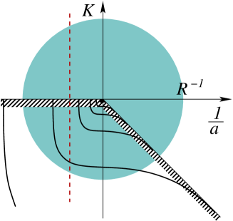
Figure 1: Illustration of the Efimov spectrum: The energy variable $K={\rm sgn}(E)\sqrt{m|E|}$ is shown as a function of the inverse scattering length $1/a$. The shaded circular region exhibits the window of universality. The solid lines indicate the Efimov states, while the hashed areas give the scattering thresholds and the dashed vertical line illustrates an exemplary system with fixed scattering length.

in the two-dimensional plane spanned by the momentum variable $K={\rm sgn}(E)\sqrt{m|E|}$ and the inverse scattering length $1/a$. The shaded circular area of radius $R^{-1}$ indicates the window of universality where range corrections are small. The solid lines indicate the Efimov states while the hashed areas give the scattering thresholds below which the bound states can exist. The dashed vertical line illustrates an exemplary system with a fixed scattering length. In the unitary limit $1/a=0$, the spectrum in Fig. 1 reduces to

$$B_{3}=e^{-2\pi n/s_{0}}\,\frac{\kappa_{*}^{2}}{m}\,,$$ (2)

where $s_{0}=1.00624...$ and the index $n$ labels the three-body states.

The spectra in Eq. (2) and Fig. 1 are invariant under discrete scaling transformations by the factor $\lambda_{0}=e^{\pi/s_{0}}$: where $n$ is any integer. This discrete scaling symmetry holds for all three-body observables. It can be seen explicitly in the analytical expression for the Phillips line at leading order,

$$a_{pd}/a=1.46-2.15\tan[s_{0}\ln(a\kappa_{*})+1.06]\,,$$ (3)

a correlation between the particle-dimer scattering length $a_{pd}$ and the three-body binding momentum $\kappa_{*}$. This universal correlation was originally observed in neutron-deuteron scattering calculations (Phillips, 1968). The manifestation of discrete scale invariance in observables is often referred to as Efimov physics.

When a fourth particle is added, no new parameters are needed for renormalization at leading order (Platter et al., 2004). As a consequence, in the universal regime all four-body observables are also governed by the discrete scaling symmetry and can be characterized by $a$ and $\kappa_{*}$. A similar behavior holds for higher-body observables. In ultracold atoms, these properties have now been experimentally verified for up to five particles. See Naidon and Endo (2017); Greene et al. (2017); Hammer et al. (2020) for recent reviews.

The universality of resonant interactions provides the guiding principle for the construction of Halo EFT. Thus the description of halos (and light nuclei, see König et al. (2017)) can be organized in an expansion around the unitary limit. The breakdown scale $M_{\rm core}$ of this approach is set by the lowest momentum degree of freedom not explicitly included in the theory. The EFT exploits the appearance of a large scattering length $a\gg 1/M_{\rm core}$, independent of the mechanism generating it. In addition to nuclear halo states, examples include ultracold atoms close to a Feshbach resonance and hadronic molecules in particle physics (Braaten and Hammer, 2007; Hammer and Platter, 2010; Naidon and Endo, 2017; Guo et al., 2018). The typical momentum scale of the theory is $M_{\rm halo}\sim 1/a\sim K$, which for the systems under consideration here is usually of order tens of MeV. Meanwhile, the Halo EFT breakdown scale, $M_{\rm\rm core}$, varies between 50 and 150 MeV, depending on the system. The expansion is then in powers of $M_{\rm halo}/M_{\rm core}$, and for a calculation to order $b$ the omitted short-range physics should affect the EFT’s answer by a fractional amount of order $(M_{\rm halo}/M_{\rm core})^{b+1}$, as long as we consider a process at a momentum of order $M_{\rm halo}$. For momenta of the order of the breakdown scale $M_{\rm core}$ the EFT expansion diverges: the omitted short-range physics is resolved and has to be treated explicitly. For many applications, the discussion of uncertainties based on such estimates is sufficient. However, a more sophisticated implementation of this prescription that employs Bayesian statistics to update the size of the error bar based on the convergence of the perturbative series is possible (Furnstahl et al., 2015).

The direct observation of the discrete scaling symmetry in the level spectra or reactions of halo nuclei would be a smoking gun for Efimov physics (Amorim et al., 1997; Jensen et al., 2004; Macchiavelli, 2015), but the contribution of higher partial waves and partial-wave mixing complicate the situation. While Halo EFT naturally accommodates resonant interactions in higher partial waves (Bertulani et al., 2002; Bedaque et al., 2003a), there is no Efimov effect in this case (Nishida, 2012; Braaten et al., 2012). Moreover, universality for resonant P-wave interactions is weaker, as two parameters, the P-wave scattering volume and effective range, are required already at leading order in the two-body system. In higher partial waves this pattern gets progressively worse (Bertulani et al., 2002; Harada et al., 2009). Nevertheless, universality still provides powerful constraints for the structure and dynamics of halo nuclei (Hammer et al., 2017).

The fact that the halo nucleons and the core are treated as distinguishable particles in Halo EFT means that the halo nucleons are not antisymmetrized with nucleons in the core—the latter are not active degrees of freedom in the EFT. This clearly introduces an error. However, the contribution of a hypothetical configuration where a nucleon from the core and from the halo are exchanged to observables is governed by the overlap of the wave functions of the core and the halo. Since the ranges of the core and halo wave functions are $1/M_{\rm core}$ and $1/M_{\rm halo}$, respectively, the size of the contribution is governed by the standard Halo EFT expansion in $M_{\rm halo}/M_{\rm core}$. Therefore, the impact of anti-symmetrization on observables is controlled by the Halo EFT expansion and can be incorporated together with that of other short-distance effects. In a single-nucleon halo, these effects enter through the low-energy constants of the nucleon-core interaction which is fitted to experimental data or ab initio input. In a two-nucleon halo, they also enter through a short-range three-body force. This can be understood as follows: the full anti-symmetrization of the wave function in a theory with active core nucleons will result in additional nodes of the halo wave function since some nucleons must be in excited states to obey the Pauli principle. In a cluster model, these additional nodes are generated by including deep unphysical bound states (ghost states) of the core and the halo, see, e.g., Baye and Descouvemont (1985). In Halo EFT such deep unphysical states are not included explicitly. The manifestation of the corresponding physics in Halo EFT can be understood by assuming that the unphysical states have been integrated out of the theory. This generates a short-range three-body force between the core and the two halo nucleons (or modifies an already existing three-body force in the theory).

Finally, we note that Halo EFT is not meant to replace ab initio approaches to halo nuclei, instead it complements ab initio approaches by providing universal relations between different halo observables. Thus it presents a unified framework for the description of different halo nuclei and their properties. On the one hand, these universal relations can be combined with inputs from ab initio theories or experiments to predict halo properties. On the other hand, they can be used to test calculations and/or measurements of different observables for their consistency.

The chapter is organized as follows. We start by writing down the effective potential of Halo EFT. This is followed by a discussion of two- and three-body halo systems with some applications. Finally, we review universality in multi-neutron systems and provide pointers to further reading on topics that have been omitted due to space constraints, including alternative approaches to halo nuclei.

2 Effective potential

In order to describe halo nuclei in a non-relativistic EFT framework, it is important to establish formulae for observables in halos that are generally suitable for all systems under consideration, and then apply these expressions to specific cases. Here, we focus on one- and two-neutron halos with S-wave interactions between the core and the valence neutrons.

We introduce an effective potential $V^{eff}$ to describe a general S-wave halo consisting of a core ($c$) with spin ${j_{c}}$ and mass $m_{c}$ and one or two valence neutrons ($n$) with spin $1/2$ and mass $m_{n}$. $V^{eff}$ is written as a sum of $N$-body potentials,

$$V^{eff}=V^{eff}_{2}+V^{eff}_{3}+\ldots\,,$$ (4)

where the dots stand for higher-body terms not needed here. The two-body S-wave neutron-neutron ($nn$) and neutron-core ($nc$) short-range interactions are represented by contact terms. The two valence neutrons interact in the spin-singlet state, which has a large negative scattering length. The neutron and the core couple into states with total spin ${s}$, whose values can be ${s}_{-}=|{j_{c}}-1/2|$ and ${s}_{+}={j_{c}}+1/2$, denoted by $nc(-)$ and $nc(+)$, respectively. In the case of a spinless core, the $nc$ interaction forms only one state with ${s}=1/2$. Due to Galilei invariance, the interaction does not depend on the center-of-mass momentum. Thus we write the two-body interaction containing both the $nn$ and $nc$ contact interactions as

$$\langle\bm{k}^{\prime}|V^{eff}_{2}|\bm{k}\rangle = \sum_{x=nn,nc(\pm)}\mathscr{P}_{x}\left(C_{0,x}+C_{2,x}(\bm{k}^{\prime 2}+\bm{k})^{2}/2+\ldots\right)\,,$$ (5)

where $C_{0,x}$, $C_{2,x}$ are coupling constants and $\mathscr{P}_{x}$ are projection operators on the corresponding two-body channels $x=nn,nc(\pm)$. Moreover, $\bm{k}$ and $\bm{k}^{\prime}$ are the relative momenta in the incoming and outgoing channels while the dots represent higher-order momentum-dependent interaction terms. A neutron halo can be formed if one of the $nc$ spin channels, $nc(+)$ or $nc(-)$, has a scattering length that is much larger than the range of the interaction. Then the Efimov scenario from the previous subsection applies.

The three-body effective potential $V^{eff}_{3}$ does not contribute in a one-neutron halo nucleus but, in our Halo EFT description of a two-neutron halo nucleus, arises from the requirement that the three-body problem be properly renormalized (Bedaque et al., 1999b, a). For simplicity, we write $V^{eff}_{3}$ using a projection operator for a specific $n$-$nc$-channel. In an S-wave $2n$ halo system whose ground state has spin $J$, $V^{eff}_{3}$ can be represented by a three-body potential coupling an $nc$ channel and a neutron $n$,

$$\langle\bm{p}^{\prime}\bm{q}^{\prime}|V^{eff}_{3}|\bm{p},\bm{q}\rangle=D_{0}\,\mathscr{P}_{n-nc(J)}+\ldots\,,$$ (6)

where $\mathscr{P}_{n-nc(J)}$ is the projection operator for the $n$-$nc$-channel with spin $J$, $D_{0}$ is the three-body coupling constant, and $\bm{p}{(^{\prime})}$, $\bm{q}{(^{\prime})}$ are Jacobi momenta. Based on the effective potential $V^{eff}$, one can calculate low-energy halo observables. The accuracy of the calculation can be progressively improved via the systematic expansion in $M_{\rm halo}/M_{\rm core}$ by adding higher order terms in $V^{eff}$. In the following we use a shorthand notation, denoting calculations done at leading, next-to-leading, and order $b$ in this expansion as LO, NLO, and N^bLO.

3 Two-body halos

The two-body amplitude in a given channel $x=nn,\,nc(\pm)$ is obtained by solving the Lippmann-Schwinger equation for the effective potential,

$$\langle\bm{k}^{\prime}|t_{x}(E)|\bm{k}\rangle = \langle\bm{k}^{\prime}|V^{eff}_{2}|\bm{k}\rangle+2\mu_{x}\int\frac{d^{3}\bm{q}}{(2\pi)^{3}}\frac{\langle\bm{k}^{\prime}|V^{eff}_{2}|\bm{q}\rangle\langle\bm{q}|t_{x}(E)|\bm{k}\rangle}{k^{2}-q^{2}+i\epsilon}\,,$$ (7)

where $E=k^{2}/(2\mu_{x})$ with $k=|\bm{k}|$ is the total kinetic energy in the center-of-mass frame. The momenta $\bm{k}^{\prime}$ and $\bm{q}$ are off-shell. Note that only the part of $V^{eff}_{2}$ acting in the channel of interest, $x$, contributes. The reduced masses are $\mu_{nn}=m_{n}/2$ and $\mu_{nc(\pm)}=Am_{n}/(A+1)$, where $A\equiv m_{c}/m_{n}$ denotes the core-neutron mass ratio.

Inserting the leading order potential we obtain

$$\langle\bm{k}^{\prime}|t_{x}(E)|\bm{k}\rangle = C_{0,x}+2\mu_{x}C_{0,x}\int\frac{d^{3}\bm{q}}{(2\pi)^{3}}\frac{\langle\bm{q}|t_{0,x}(E)|\bm{k}\rangle}{k^{2}-q^{2}+i\epsilon}\,.$$ (8)

This integral equation is depicted diagrammatically in Fig. 2.

Figure 2: Integral equation for the two-body amplitude (1st line) and perturbative solution (2nd line). The effective potential is represented by the filled circle, while the blob indicates the scattering amplitude.

Perturbation theory in $C_{0,x}$ leads to a geometric series which can be summed up to obtain the exact nonperturbative solution:

$$\langle\bm{k}^{\prime}|t_{x}(E)|\bm{k}\rangle = C_{0,x}+C_{0,x}IC_{0,x}+C_{0,x}IC_{0,x}IC_{0,x}+\ldots=[1/C_{0,x}-I]^{-1}\,,$$ (9)

where

$$I = 2\mu_{x}\int\frac{d^{3}\bm{q}}{(2\pi)^{3}}[k^{2}-q^{2}+i\epsilon]^{-1}\,.$$ (10)

The Integral $I$ is formally divergent and needs to regularized. This can, e.g., be done by cutting the integral off at high momenta, using dimensional regularization with power-law divergence subtraction (PDS) (Kaplan et al., 1998), or an arbitrary regularization scheme (van Kolck, 1999). For simplicity, we apply a sharp momentum cutoff $\Lambda\gg k$ on the absolute value of $\bm{q}$ and obtain:

$$I = -\frac{\mu_{x}}{2\pi}\left(ik+\frac{2}{\pi}\Lambda+\mathscr{O}(k^{2}/\Lambda)\right)\,,$$ (11)

where the terms of $\mathscr{O}(k^{2}/\Lambda)$ can be dropped.

The resulting amplitude has the same structure as the effective range expansion (ERE) of the two-body S-wave scattering amplitude in the channel $x$,

$$\langle\bm{k}^{\prime}|t_{x}(E)|\bm{k}\rangle=\frac{2\pi}{\mu_{x}}\left[\frac{1}{a_{x}}+ik\right]^{-1}\,,$$ (12)

with terms of $\mathcal{O}(k^{2})$ being omitted. Moreover, $|\bm{k}|=|\bm{k}^{\prime}|=k=\sqrt{2\mu_{x}E}$ in Eq. (12) is the on-shell relative momentum of the two particles in the center-of-mass frame. $a_{x}$ indicates the large S-wave scattering length in the channel $x$, which is related to the low-momentum scale by $a_{x}\sim 1/M_{\rm halo}$. For typical momenta $k\sim M_{\rm halo}$, higher-order corrections are suppressed by $M_{\rm halo}/M_{\rm core}$.

We use Eq. (12) as a renormalization condition to determine the running coupling $C_{x}(\Lambda)$ and obtain

$$C_{0,x}(\Lambda) = \frac{2\pi}{\mu_{x}}\left[\frac{1}{a_{x}}-\frac{2}{\pi}\Lambda\right]^{-1}\,.$$ (13)

Note also that the unitary term $ik$ does not require regularization, since it arises from on-shell intermediate states in Eq. (8).

The momentum-dependent $C_{2,x}$ term from Eq. (5) can be included by writing $C_{0,x}+C_{2,x}(\bm{k}^{\prime 2}+\bm{k})^{2}/2$ as a two-term separable potential (see, e.g., Beane et al. (1998) for details). Solving the corresponding Lippman-Schwinger equation, we obtain the scattering amplitude with effective range term $r_{x}$,

$$\langle\bm{k}^{\prime}|t_{x}(E)|\bm{k}\rangle=\frac{2\pi}{\mu_{x}}\left[\frac{1}{a_{x}}-\frac{r_{x}}{2}k^{2}+ik\right]^{-1}\,.$$ (14)

Note, however, that the Wigner causality bound limits the range of cutoffs $\Lambda$ that can be used if one wants to reproduce a positive effective range, $r_{x}>0$ (Phillips and Cohen, 1997; Hammer and Lee, 2010).

For our application to S-wave halo nuclei, which exhibit shallow bound or virtual states, we are interested in the case of a large scattering length, $|a_{x}|\gg|r_{x}|$ in the channel $x$. The scattering amplitude $t_{x}$ can then be expanded around the low-energy pole at $k=i\gamma_{x}$, where $\gamma_{x}$ is the binding momentum of the two-body S-wave bound state ($\gamma_{x}>0$) or virtual state ($\gamma_{x}<0$). At the level of accuracy of Eq. (14), the binding momentum is related to the scattering length $a_{x}$ and the effective range $r_{x}$ by

$$\frac{1}{a_{x}}=\gamma_{x}-\frac{r_{x}}{2}\gamma_{x}^{2}\,.$$ (15)

Therefore, physics of scale $k\sim|\gamma_{x}|$ is enhanced due to the pole structure of the scattering amplitude. The EFT is constructed based on a systematic expansion in $\gamma_{x}r_{x}$ or $r_{x}/a_{x}$. In the zero-range limit ($r_{x}=0$) or in the unitary limit ($a_{x}\rightarrow\pm\infty$), we have $\gamma_{x}=1/a_{x}$: the leading order of the EFT expansion in Eq. (15) then becomes exact.

Near the pole, the scattering amplitude, Eq. (14), can be expanded about the pole at $E=-\gamma_{x}^{2}/(2\mu_{x})$:

$$\langle\bm{k}^{\prime}|t_{x}(E)|\bm{k}\rangle=\frac{Z_{x}}{E+\gamma_{x}^{2}/(2\mu_{x})}+{\rm regular}\,,$$ (16)

with the residue of the pole

$$Z_{x}=\lim_{E\to-\gamma_{x}^{2}/(2\mu_{x})}\;\left(E+\frac{\gamma_{x}^{2}}{2\mu_{x}}\right)\,t_{x}(E)=\frac{\pi}{\mu_{x}^{2}}\frac{2\gamma_{x}}{1-\gamma_{x}r_{x}}\,.$$ (17)

In a bound two-body system, the residue $Z_{x}$ is connected to the asymptotic normalization coefficient (ANC) $A_{x}$ of the bound-state wave function. Near the bound state pole, the full Green’s function has the general form

$$\langle\bm{k}^{\prime}|\frac{1}{E-H}|\bm{k}\rangle=\frac{\psi_{x}(\bm{k}^{{}^{\prime}})\psi_{x}^{*}(\bm{k})}{E+\gamma_{x}^{2}/(2\mu_{x})}+{\rm regular}\,,$$ (18)

where $\psi_{x}(\bm{k})$ is the asymptotic wave function for the S-wave bound state in the channel $x$, whose co-ordinate space representation is

$$\psi_{x}(\bm{r})=A_{x}Y_{00}({\hat{r}})\frac{\exp(-\gamma_{x}r)}{r}\,,$$ (19)

with the ANC $A_{x}$ and $Y_{00}({\hat{r}})=1/\sqrt{4\pi}$ a spherical harmonic. To relate $A_{x}$ to $Z_{x}$, we write the full Green’s function in terms of the free Green’s function $1/(E-H_{0})$ and $t_{x}(E)$ as

$$\frac{1}{E-H}=\frac{1}{E-H_{0}}+\frac{1}{E-H_{0}}t_{x}(E)\frac{1}{E-H_{0}}\,.$$ (20)

Any bound-state pole can only come from the second piece on the right-hand side of Eq. (20). Going to the momentum representation and using the expression for $\langle\bm{k}^{\prime}|t_{x}(E)|\bm{k}\rangle$ near the pole from Eq. (16) together with Eqs. (18, 19), we obtain the relation

$$A_{x}=\frac{\mu_{x}}{\sqrt{\pi}}\sqrt{Z_{x}}=\sqrt{\frac{2\gamma_{x}}{1-\gamma_{x}r_{x}}}\,.$$ (21)

Therefore, one can use the ANC $A_{x}$ and the binding momentum $\gamma_{x}$ to determine the EFT parameters $C_{0,x}$ and $C_{2,x}$, instead of fixing them from the scattering parameters $a_{x}$ and $r_{x}$. At LO, $A_{x}=\sqrt{2\gamma_{x}}$ is determined by the binding momentum. At NLO, the effect of a finite effective range enters and produces an ANC ratio different from one:

$$A_{x}/A_{x,LO}=\left(1-\gamma_{x}r_{x}\right)^{-1/2}\,.$$ (22)

Note that $A_{x}/A_{x,LO}>1$ if $\gamma_{x}>0$ (i.e. the two-body system $x$ is bound) and $r_{x}>0$. The extent to which this ratio deviates from one then indicates the importance of range effects.

Although $A_{x}$ is not an observable that is directly measured in scattering experiments, it can be extracted from such data by an analytic continuation of the scattering amplitude to negative energies. There $t_{x}$ has the pole structure

$$\langle\bm{k}^{\prime}|t_{x}(E)|\bm{k}\rangle=\frac{2\pi}{\mu_{x}}\frac{A^{2}_{x}/A^{2}_{x,LO}}{\gamma_{x}+ik}+\rm{regular}\,.$$ (23)

As compared to the ERE, which is an expansion in powers of $r_{x}/a_{x}$ around $k=0$, this parameterization in terms of an ANC, dubbed the z-parameterization by Phillips et al. (2000), is a more convenient choice for bound-state calculations. Using this parameterization, the pole at $k=i\gamma_{x}$ is exactly reproduced at each order, and the residue of the scattering amplitude, $A^{2}_{x}/A^{2}_{x,LO}$, is expanded into a LO piece $=1$ and an NLO piece $=(A^{2}_{x}/A^{2}_{x,LO}-1)$. N²LO and higher corrections to the ANC are then zero by definition. The $z$-parameterization of the scattering amplitude is accurate at relative order $(M_{\rm halo}/M_{\rm core})^{2}$, beyond which the shape parameter enters at $\mathcal{O}(k^{4})$.

Here we illustrate the utility of the $z$-parameterization in the calculation of the matter form factor of one-neutron halos, i.e., we now choose $x=nc$. The neutron-core form factor is the Fourier transform of the coordinate-space probability density distribution:

$$F_{nc}(|\bm{q}|)=\int d^{3}r|\psi_{nc}(\bm{r})|^{2}\exp(i\bm{q}\cdot\bm{r})\,.$$ (24)

At LO, we use the zero-range two-body wave function by inserting $A_{x,LO}=\sqrt{2\gamma_{x}}$ in Eq. (19) and obtain

$$F_{nc}^{(LO)}(|\bm{q}|)=\frac{2\gamma_{nc}}{|\bm{q}|}\arctan\left(\frac{|\bm{q}|}{2\gamma_{nc}}\right)\,.$$ (25)

The form factor $F_{nc}^{(NLO)}$ is calculated from Eq. (24) using the full ANC, $A_{nc}$, with an additional insertion of a constant piece that ensures the matter form factor is properly normalized (Phillips et al., 2000; Chen et al., 1999), i.e., $F_{nc}(0)=1$. Consequently, the NLO correction to $F_{nc}$ is

$$F_{nc}^{(NLO)}(|\bm{q}|)=-(A^{2}_{nc}/A^{2}_{nc,LO}-1)\left[1-\frac{2\gamma_{nc}}{|\bm{q}|}\arctan\left(\frac{|\bm{q}|}{2\gamma_{nc}}\right)\right]\,.$$ (26)

Since the low-momentum expansion of the form factor in the one-neutron halo is related to the mean squared distance between the neutron and the core $\langle r_{nc}^{2}\rangle$ via

$$F_{nc}(|\bm{q}|)=1-\frac{1}{6}\langle r^{2}\rangle_{nc}\bm{q}^{2}+\mathcal{O}(\bm{q}^{4})\,,$$ (27)

we obtain $\langle r^{2}\rangle_{nc}$ by calculating the first-order derivative of $F_{nc}$ with respect to $q^{2}$ at zero. $\langle r^{2}\rangle_{nc}^{1/2}$ at NLO is then

$$\langle r^{2}\rangle_{nc}^{1/2}=\frac{A_{nc}/A_{nc,LO}}{\sqrt{2}\gamma_{nc}}\,,$$ (28)

which reproduces the LO result, Eq. (1).

With the neutron-core radius in hand we can calculate the matter radius, which is defined, in the point-nucleon limit, as the average distance-squared from all nucleons in a halo nucleus to the center of mass (Tanihata et al., 2013):

$$\langle r_{m}^{2}\rangle_{1n\rm-halo}=\frac{A}{(A+1)}\langle r_{m}^{2}\rangle_{\rm core}+\frac{A}{(A+1)^{2}}\langle r^{2}\rangle_{nc}\,,$$ (29)

where the first term is the correction from the matter radius of the core.

A more formal method of keeping the normalization $F_{nc}(0)=1$ involves imposing gauge invariance of the Lagrangian in the presence of an external gauge field. For a discussion of external gauge fields as well as the form factors of bound states with higher angular momenta, we refer the reader to Hammer and Phillips (2011); Braun et al. (2019).

3.1 Applications 1: bound S-wave neutron halos

As an application, we consider some examples of one-neutron S-wave halos, whose properties are listed in Table 1. We use $S_{1n}\equiv\textrm{sgn}(\gamma_{nc})\gamma_{nc}^{2}/(2\mu_{nc})$ to denote the neutron-core separation energy in a one-neutron halo, with $S_{1n}>0$ ($<0$) corresponding to a bound (virtual) S-wave state.

	2H	11Be	15C	19C
Experiment
$J^{P}$	$1^{+}$	$1/2^{+}$	$1/2^{+}$	$1/2^{+}$
$S_{1n}$ [MeV]	2.224573(2)	0.50164(25)	1.2181(8)	0.58(9)
$E^{*}_{c}$ [MeV]	293	3.36803(3)	6.0938(2)	1.62(2)
$\langle r^{2}\rangle_{nc}^{1/2}$ [fm]	3.936(12)	6.05(23)	4.15(50)	6.6(5)
	3.95014(156)	5.7(4)	7.2(4.0)	6.8(7)
		5.77(16)	4.5(5)	5.8(3)
Halo EFT
$M_{\rm halo}/M_{\rm core}$	0.33	0.39	0.45	0.6
$r_{nc}/a_{nc}$	0.32	0.38	0.43	0.33
$A_{nc}/A_{nc,LO}$	1.295	1.44	1.63	1.3
$r_{nc}$ [fm]	1.7436(19)	3.5	2.67	2.6
$\langle r^{2}\rangle_{nc,{\rm theo}}^{1/2}$ [fm]	3.954	6.85	4.93	5.72

Table 1: Properties of S-wave one-neutron halos. One-neutron separation energy $S_{1n}$ taken from AME2012 (Audi et al., 2012; Wang et al., 2012), while lowest core excitation energies $E^{*}_{c}$ for $A>1$ halos are from the TUNL database (Ajzenberg-Selove, 1987; Tilley et al., 2004; Ajzenberg-Selove, 1991). $M_{\rm halo}$ and $M_{\rm core}$ are estimated using $S_{1n}$ and $E^{*}_{c}$ except for the deuteron (see text). Different experimental values of $\langle r^{2}\rangle_{nc}^{1/2}$ are given (errors in parentheses). For a discussion of theoretical uncertainties, see main text. Compilation taken from (Hammer et al., 2017) where also a complete list of references can be found.

The deuteron has a spin-triplet ground state ($J^{P}=1^{+}$), which is dominated by an S-wave component. The deuteron binding energy as determined by the 2012 Atomic Mass Evaluation (AME2012) (Audi et al., 2012; Wang et al., 2012) is $S_{1n}=2.224573(2)$ MeV. In the language of Halo EFT, the low scale here is $M_{\rm halo}\sim\gamma_{nc}=\sqrt{m_{n}S_{1n}}=45.7$ MeV. An estimate of the high scale is obtained from the exchange of pions among nucleons, $M_{\rm core}\sim M_{\pi}$. Well below the pion mass, nuclear potentials can be considered as short ranged by integrating out the pion degrees of freedom. Such a pionless EFT calculation of the deuteron is then based on the expansion parameter $M_{\rm halo}/M_{\rm core}\approx 1/3$. The low energy physics of the deuteron can also be related to $np$ scattering data. In the S-wave spin-triplet channel, the scattering parameters $a_{{}^{3}S_{1}}=5.4112(15)$ fm and $r_{{}^{3}S_{1}}=1.7436(19)$ fm are determined from an analysis of $np$ elastic scattering data (Hackenburg, 2006). Their values indicate that the effective range is of expected size ($r_{{}^{3}S_{1}}\sim 1/M_{\rm core}\sim 1/M_{\pi}$) while the scattering length is large, i.e., $a_{{}^{3}S_{1}}\sim 1/M_{\rm halo}$, leading to an expansion parameter consistent with the estimate from bound state properties above.

Using Eq. (21) we obtain the ANC for the deuteron S-wave wave function to be $A_{{}^{3}S_{1}}=1.295$ (Phillips et al., 2000). The deuteron structure radius in the point-nucleon limit, equivalent to $\langle r^{2}\rangle_{np}^{1/2}/2$, follows from Eq. (28) as $1.977$ fm, which overlaps with the value extracted from elastic electron-deuteron scattering (Herrmann and Rosenfelder, 1998) and agrees with calculations based on realistic nucleon-nucleon potentials (Friar et al., 1997).

Another example of a one-neutron halo is ¹⁹C, whose ground state was determined from the Coulomb dissociation spectrum (Nakamura et al., 1999) to be $J^{P}=1/2^{+}$, with a separation energy $S_{1n}=0.53(13)$ MeV between the ¹⁸C core ($J^{P}=0^{+}$) and the last neutron. This result is consistent with $S_{1n}=0.65(15)$ MeV from one-neutron knock out reactions (Maddalena et al., 2001), and $S_{1n}=0.58(9)$ MeV in AME2012. The first excitation energy of ¹⁸C is $E^{*}_{c}=1.62(2)$ MeV (Ajzenberg-Selove, 1987). These values suggest a separation of low and high scales by $M_{\rm halo}/M_{\rm core}\sim\sqrt{S_{1n}/E^{*}_{c}}\approx 0.6$. Acharya and Phillips (2013) performed an EFT analysis on the ¹⁹C Coulomb dissociation data (Nakamura et al., 1999, 2003). They extracted $A_{nc}/A_{nc,LO}=1.31$, together with $S_{1n}=0.575(55)(20)$ MeV—the latter in agreement with the extraction by Nakamura et al. (1999) and AME2012. These correspond to ERE parameters $a_{nc}=7.75(35)(30)$ fm and $r_{nc}=2.6^{+0.6}_{-0.9}\pm 0.1$ fm, where the first error indicates the statistical uncertainty from the fit to data and the second one quantifies the systematic N³LO EFT uncertainties, which are estimated to be of relative size $(r_{nc}/a_{nc})^{3}$. In fact, the ratio $r_{nc}/a_{nc}=0.33$ suggests that the EFT may converge faster than the naive dimensional estimate, $M_{\rm halo}/M_{\rm core}\approx 0.6$.

The above results for ¹⁹C imply an S-wave binding momentum $\gamma_{nc}=32.0$ MeV. This, together with the extracted ANC, yields the neutron-core distance from Eq. (28) to be $\langle r^{2}\rangle_{nc}^{1/2}=5.72$ fm, which agrees with values deduced by the E1 sum rule of Coulomb dissociation (Nakamura et al., 1999) and extracted from the charge-changing cross section (Kanungo et al., 2016) measurements (see Table 1).

Other examples of one-neutron halos are ¹¹Be and ¹⁵C. Their ground states both have spin-parity quantum numbers $J^{P}=1/2^{+}$, with one valence neutron attached to the ¹⁰Be and ¹⁴C cores ($J^{P}=0^{+}$). The one-neutron separation energies $S_{1n}$ of ¹¹Be and ¹⁵C are given in the atomic mass evaluation AME2012; while the first excitation energies of the cores $E_{c}^{*}$ are obtained from the TUNL data base (Tilley et al., 2004; Ajzenberg-Selove, 1991), cf. Table 1.

Based on naive dimensional analysis the EFT expansion parameter in ¹¹Be is $M_{\rm halo}/M_{\rm core}\sim\sqrt{S_{1n}/E^{*}_{c}}=0.39$. The ANC in the ¹¹Be ground state was obtained in an ab initio calculation that used the No-Core Shell Model with Continuum approach as $A_{nc}/A_{nc,LO}=1.44$ (Calci et al., 2016). This corresponds to $r_{nc}=3.5$ fm, which yields $r_{nc}/a_{nc}=0.38$ in ¹¹Be, in agreement with the expansion parameter inferred from $\sqrt{S_{1n}/E^{*}_{c}}$.

EFT calculations for ¹⁵C were performed in (Rupak et al., 2012; Fernando et al., 2015). By fitting the Halo EFT neutron capture cross section to experiment (Nakamura et al., 2009), they determined the ANC ratio $A_{nc}/A_{nc,LO}=1.63$, or equivalently, an effective range $r_{nc}=2.67$ fm. Their calculation suggested an unnaturally scale for the effective range, with $r_{nc}\sim 1/M_{\rm halo}$, implying that the z-parameterization, $A_{nc}^{2}/A_{nc,LO}^{2}-1$, becomes non-perturbative in this system. Using the ANC extracted in (Rupak et al., 2012), we obtain $r_{nc}/a_{nc}=0.43$, which, despite the somewhat large effective range, is still consistent with $M_{\rm halo}/M_{\rm core}\approx 0.45$.

3.2 Applications 2: unbound S-wave neutron halos

Halo-like features also exist in unbound systems, if such systems display a large negative scattering length. In the $np$ spin singlet state, the ERE parameters $a_{{}^{1}S_{0}(np)}=-23.7148(43)$ fm and $r_{{}^{1}S_{0}(np)}=2.750(18)$ fm are determined from at analysis of low-energy $np$ elastic-scattering data (Hackenburg, 2006). The $nn$ singlet state is also unbound, with a scattering length $a_{{}^{1}S_{0}(nn)}=-18.6(5)$ fm and $r_{{}^{1}S_{0}(nn)}=2.83(11)$ fm obtained from the neutron time-of-flight spectrum in radiative pion capture on the deuteron (Chen et al., 2008). It should be noted, however, that there is a systematic and significant difference between the extracted values of $a_{{}^{1}S_{0}(nn)}$ from neutron-induced deuteron breakup reactions measured by two different collaborations with different experimental setups (Gardestig, 2009). A Halo EFT analysis of the reaction ⁶He$(p,p\alpha)nn$ in inverse kinematics at high energies may help to resolve this discrepancy (Göbel et al., 2021). Further below we will also discuss some universal features of unbound multineutron systems based on the fact that $r_{{}^{1}S_{0}}/a_{{}^{1}S_{0}}$ is a small parameter (Hammer and Son, 2021).

¹¹Li, whose ground state has spin-parity $J^{P}=3/2^{-}$ was one of the first halo nuclei (Tanihata et al., 1985) beyond the few-nucleon systems to be discovered. ¹¹Li is a Borromean two-neutron halo, where the neutron-core is unbound. Here we focus on the separation of scales in ¹⁰Li and refer to later sections for properties of ¹¹Li. The ground state of the ⁹Li core has $J^{P}=3/2^{-}$ and a first excitation energy $E^{*}_{c}=2.691(5)$ MeV (Tilley et al., 2004), which sets $M_{\rm core}$. The scale $M_{\rm halo}$ is associated with the ¹⁰Li ground state, which can be interpreted as an unbound S-wave neutron-core virtual state ($J^{P}=1^{-}$ or $2^{-}$) with $S_{1n}=-25(15)$ keV (Tilley et al., 2004). The EFT expansion parameter for ¹⁰Li is estimated as $M_{\rm halo}/M_{\rm core}\sim\sqrt{|S_{1n}|/E^{*}_{c}}\approx 0.1$. A proton removal reaction experiment (Smith et al., 2015) observed two resonance states of ¹⁰Li at energies $E_{2,1+}=110(40)$ keV and $E_{2,2+}=500(100)$ keV above the neutron-core threshold. These are expected to be P-wave states. As such they enter at higher orders in the EFT compared to the S-wave virtual state, whose large scattering length promotes it to LO.

²¹C is another unbound neutron-core system (Langevin et al., 1985). The ratio between the one-neutron separation energies of ²¹C and ²⁰C from AME2012 provides a valid expansion parameter $\mathrel{\hbox to0.0pt{\lower 4.0pt\hbox{\hskip 1.0pt$\sim$}\hss}\raise 1.0pt\hbox{$<$}}0.18$. The neighboring isotope ²²C has recently been identified as a weakly-bound two-neutron halo and is the dripline nucleus of carbon isotopes. A Glauber-model analysis of the reaction cross section of ²²C on a hydrogen target (Tanaka et al., 2010) and a measurement of the two-neutron removal reaction on ²²C (Kobayashi et al., 2012) suggest that $n-^{20}$C is preferentially in $1/2^{+}$ configuration. The two-neutron halo structure of ²²C implies that ²¹C occupies an S-wave virtual state near the unitary limit. However, a recent study of the $n-^{21}$C decay spectrum via one-proton removal from the ²²N beam (Mosby et al., 2013) implies that the $n-^{20}$C scattering length is not large, $|a_{nc}|<2.8$ fm (or equivalently $S_{1n}<-2.8$ MeV). Therefore, further studies on the properties of ²¹C are needed.

4 Three-body halos

Here we consider two-neutron halos as a neutron-neutron-core three-body system. We use the Jacobi momentum plane-wave state $|\boldsymbol{p},\boldsymbol{q}\rangle_{i}$ to represent the kinematics of the three-body system in the center-of-mass frame. The index $i$ indicates that these momenta are defined in the two-body fragmentation channel $(i,jk)$, in which particle $i$ is the spectator and $(jk)$ the interacting pair. Based on this definition, $\boldsymbol{p}$ represents the relative momentum in the pair $(jk)$; while $\boldsymbol{q}$ denotes the relative momentum between the spectator $i$ and the $(jk)$ pair. The plane-wave states are normalized as (Glöckle, 1983):

$${}_{i}\langle\bm{p}\bm{q}|\bm{p}^{\prime}\bm{q}^{\prime}\rangle_{i}=(2\pi)^{6}\delta^{(3)}(\bm{p}-\bm{p}^{\prime})\delta^{(3)}(\bm{q}-\bm{q}^{\prime})\,.$$ (30)

The Jacobi momenta are related to the momenta in the direct product of three single-particle states $|\bm{k}_{1},\bm{k}_{2},\bm{k}_{3}\rangle$ in the center-of-mass frame (i.e., $\bm{k}_{1}+\bm{k}_{2}+\bm{k}_{3}=0$) by

$$\langle\bm{k}_{1},\bm{k}_{2},\bm{k}_{3}|\bm{p}\bm{q}\rangle_{i} = (2\pi)^{6}\delta^{(3)}\left(\bm{p}_{i}-\mu_{jk}\left[\frac{\bm{k}_{j}}{m_{j}}-\frac{\bm{k}_{k}}{m_{k}}\right]\right)\,$$ (31)

$$\qquad\times\delta^{(3)}\left(\bm{q}_{i}-\mu_{i(jk)}\left[\frac{\bm{k}_{i}}{m_{i}}-\frac{\bm{k}_{j}+\bm{k}_{k}}{M_{jk}}\right]\right)\,,$$

where $M_{jk}=m_{j}+m_{k}$, $\mu_{jk}=m_{j}m_{k}/M_{jk}$, and $\mu_{i(jk)}=m_{i}M_{jk}/(m_{i}+M_{jk})$ are mass parameters.

To discuss the spin and parity of a halo nucleus, we introduce the partial-wave-decomposed representation. The relative orbital angular momentum and the spin of the pair $(jk)$ are defined as $l_{i}$ and $s_{i}$. They are coupled to form the total angular momentum $j_{i}$ in the pair. We also define the spin of the spectator $i$ as $\sigma_{i}$, the relative orbital angular momentum between the spectator $i$ and the pair $(jk)$ as $\lambda_{i}$, and the corresponding total angular momentum as $I_{i}$. The overall orbital angular momentum, spin and total angular momentum of the three-body system are denoted by $L_{i}$, $S_{i}$ and $J$. We then have:

$$\bm{L}_{i}= \bm{l}_{i}+\bm{\lambda}_{i}\,,\quad\bm{S}_{i}=\bm{s}_{i}+\bm{\sigma}_{i}\,,\quad\bm{J}=\bm{L}_{i}+\bm{S}_{i}=\bm{j}_{i}+\bm{I}_{i}\,.$$ (32)

Knowing the spin and orbital-angular-momentum quantum numbers, we can construct three-body eigenstates with respect to the spin and orbital-angular-momentum operators. Note that $J$ is a conserved quantum number, which is independent of the choice of partition representations given in Eq. (32). We decompose the Jacobi momenta with respect to these spin and orbital- and total-angular-momentum quantum numbers by (Glöckle, 1983)

$$\left|p,q;\Omega_{i}\right\rangle_{i}=\sum\limits_{L_{i}S_{i}}\sqrt{\widehat{j}_{i}\widehat{I}_{i}\widehat{L}_{i}\widehat{S}_{i}}\,\left\{\begin{array}[]{ccc}l_{i}&s_{i}&j_{i}\\ \lambda_{i}&\sigma_{i}&I_{i}\\ L_{i}&S_{i}&J\end{array}\right\}\,\left|p,q;(l_{i},\lambda_{i})L_{i}\,;\left(s_{i},\sigma_{i}\right)S_{i}\,;(L_{i}S_{i})J\right\rangle_{i}\,,$$ (33)

where $\widehat{j}_{i}$ denotes $2{j}_{i}+1$ (the same holds for $\widehat{I}_{i}$, $\widehat{L}_{i}$ and $\widehat{S}_{i}$), $p\equiv|\bm{p}|$, and $q\equiv|\bm{q}|$. The collective symbol $\Omega_{i}$ represents all conserved spin, orbital- and total-angular-momentum quantum numbers in the partition $(i,jk)$.

In this chapter, we focus on S-wave two-neutron halos, where $l_{i}=\lambda_{i}=L_{i}=0$ and the values of the total angular momenta are equal to their corresponding spins. Therefore, one can use the spins alone to represent the decomposed plane-wave state in S-wave $2n$ halos as $|p,q;(s_{i},\sigma_{i})S\rangle_{i}$, where the three-body total spin $S$ is the same in different partitions. In the $(c,nn)$ partition, $S=\sigma_{c}$ since the two-neutron pair is spin singlet ($s_{c}=0$). Therefore, in the $(n,nc)$ partition, the neutron-core pair with spin $s_{n}=|\sigma_{c}\pm 1/2|$ couples with the second neutron with spin $\sigma_{n}=1/2$ to form the three-body total spin $S=\sigma_{c}$.

Moreover, we assume that the neutron-core states with $s_{n}=|\sigma_{c}\pm 1/2|$ are degenerate and have equal scattering lengths. Under this assumption, the three-body formalism in S-wave halos with a spin-zero core becomes general for an arbitrary S-wave two-neutron halo with spin $\sigma_{c}$. We use the Faddeev formalism (Faddeev, 1961; Glöckle, 1983; Afnan and Thomas, 1977) and decompose the three-body wave function into components. In Halo EFT, $2n$-halo nuclei are described by the transition amplitudes, $\mathcal{A}_{c}$ and $\mathcal{A}_{n}$, connecting the spectator and the interacting pair to the three-body bound state. $\mathcal{A}_{c}$ and $\mathcal{A}_{n}$ are represented by functions of the Jacobi momentum $\bm{q}$ between the spectator and the pair, and are the solution of coupled-channel homogeneous integral equations (Canham and Hammer, 2008; Acharya et al., 2013) which are illustrated with Feynman diagrams in Fig. 3.

Figure 3: The integral equations for the transition amplitudes $\mathcal{A}_{c}$ (shaded circle) and $\mathcal{A}_{n}$ (empty circle). The solid (dashed) lines represent neutrons (core), while the double (thick solid) lines represent $nn$ ($nc$) scattering amplitudes, respectively. The last piece represents the contribution from the $nnc$ three-body force.

At leading order, one can take $r_{x}\rightarrow 0$ for $x=nn,nc$ and obtains (Hammer et al., 2017),

$$\mathcal{A}_{c}(\bm{q}) = 2\int\frac{d^{3}q}{4\pi^{2}}\,G_{0}^{n}\left(\pi_{2}(\bm{q}^{\prime},\bm{q}),q;B_{3}\right)\,\tau_{nc}(q^{\prime};B_{3})\,\mathcal{A}_{n}(\bm{q}^{\prime})\,,$$

$$\mathcal{A}_{n}(\bm{q}) = \int\frac{d^{3}q^{\prime}}{4\pi^{2}}\,G_{0}^{n}\left(\pi_{2}(\bm{q},\bm{q}^{\prime}),q^{\prime};B_{3}\right)\,\tau_{nn}(q^{\prime};B_{3})\,\mathcal{A}_{c}(\bm{q}^{\prime})$$ (34)

$$+\int\frac{d^{3}q^{\prime}}{4\pi^{2}}\,\left[G_{0}^{c}\left(\pi_{3}(\bm{q}^{\prime},\bm{q}),q;B_{3}\right)+\frac{H(\Lambda)}{\Lambda^{2}}\right]\,\tau_{nc}(q^{\prime};B_{3})\,\mathcal{A}_{n}(\bm{q}^{\prime})\,,$$

where $G_{0}^{c}$ and $G_{0}^{n}$ are the three-body Green’s functions expressed in two different partitions:

$$G_{0}^{c}(p,q;B_{3}) = \left(m_{n}B_{3}+\frac{A+1}{2A}p^{2}+\frac{A+2}{2(A+1)}q^{2}\right)^{-1}\,,$$

$$G_{0}^{n}(p,q;B_{3}) = \left(m_{n}B_{3}+p^{2}+\frac{A+2}{4A}q^{2}\right)^{-1}\,.$$ (35)

The momentum variables $\bm{\pi}_{1}$, $\bm{\pi}_{2}$ and $\bm{\pi}_{3}$ are defined as

$$\bm{\pi}_{1}(\bm{q},\bm{q}^{\prime})=\bm{q}+A\bm{q}^{\prime}/(A+1)\,,$$

$$\bm{\pi}_{2}(\bm{q},\bm{q}^{\prime})=\bm{q}+\bm{q}^{\prime}/2\,,$$

$$\bm{\pi}_{3}(\bm{q},\bm{q}^{\prime})=\bm{q}+\bm{q}^{\prime}/(A+1)\,.$$ (36)

Moreover, the functions $\tau_{x}(q;B_{3})$ with $x=nn,nc$ in the three-body integral equations (34) are rescaled two-body scattering amplitudes from Eq. (12),

$$\tau_{nn}(q;B_{3}) = \frac{2}{-\gamma_{nn}+\sqrt{m_{n}B_{3}+\frac{A+2}{4A}q^{2}}}\,,$$

$$\tau_{nc}(q;B_{3}) = \frac{(A+1)/A}{-\gamma_{nc}+\sqrt{\frac{A}{A+1}\left(2m_{n}B_{3}+\frac{A+2}{A+1}q^{2}\right)}}\,,$$ (37)

while $H(\Lambda)$ is a dimensionless three-body force parameter that emerges from including the three-body interaction $D_{0}\propto m_{n}C_{0,nc}^{2}H(\Lambda)/\Lambda^{2}$ from Eq. (6). Note that our amplitudes $\mathcal{A}_{c}$ and $\mathcal{A}_{n}$ correspond to the amplitudes $\tilde{\mathcal{A}}_{c}$ and $\tilde{\mathcal{A}}_{n}$ in (Hammer et al., 2017).

By projecting the three-body transition amplitudes to S-waves, we simplify the integral equations to the expressions given in (Canham and Hammer, 2008; Acharya et al., 2013)

$$\mathcal{A}_{c}(q) = \frac{2}{\pi}\int^{\Lambda}_{0}dq^{\prime}\,q^{\prime 2}K^{n}(q^{\prime},q;B_{3})\,\tau_{nc}(q^{\prime};B_{3})\,\mathcal{A}_{n}(q^{\prime})\,,$$

$$\mathcal{A}_{n}(q) = \frac{1}{\pi}\int^{\Lambda}_{0}dq^{\prime}\,q^{\prime 2}K^{n}(q,q^{\prime};B_{3})\,\tau_{nn}(q^{\prime};B_{3})\,\mathcal{A}_{c}(q^{\prime})$$ (38)

$$+\frac{1}{\pi}\int^{\Lambda}_{0}dq^{\prime}\,q^{\prime 2}\left[K^{c}(q^{\prime},q;B_{3})+\frac{H(\Lambda)}{\Lambda^{2}}\right]\,\tau_{nc}(q^{\prime};B_{3})\,\mathcal{A}_{n}(q^{\prime})\,,$$

where a sharp momentum cutoff $\Lambda$ has been applied as a regulator. This ensures that the integral equations (38) have a unique solution. The kernel functions are

$$K^{n}(q,q^{\prime};B_{3}) = \frac{1}{2}\int_{-1}^{1}d(\hat{\bm{q}}\cdot\hat{\bm{q}}^{\prime})G_{0}^{n}\left(\pi_{2}(\bm{q},\bm{q}^{\prime}),q^{\prime};B_{3}\right)=-\frac{1}{qq^{\prime}}\textrm{Q}_{0}(z_{nc})\,,$$

$$K^{c}(q,q^{\prime};B_{3}) = \frac{1}{2}\int_{-1}^{1}d(\hat{\bm{q}}\cdot\hat{\bm{q}}^{\prime})G_{0}^{c}\left(\pi_{3}(\bm{q},\bm{q}^{\prime}),q^{\prime};B_{3}\right)=-\frac{A}{qq^{\prime}}\textrm{Q}_{0}(z_{nn})\,,$$ (39)

with $\textrm{Q}_{l}$ the Legendre function of the second kind, which is related to the Legendre polynomial $P_{l}$ by $\textrm{Q}_{l}(z)\equiv\frac{1}{2}\int^{1}_{-1}dx\,P_{l}(x)/(z-x)$. The arguments $z_{nn}$ and $z_{nc}$ of $\textrm{Q}_{0}$ in Eqs. (39) are defined as

$$z_{nc} = -\frac{1}{qq^{\prime}}\left(m_{n}B_{3}+q^{2}+\frac{A+1}{2A}q^{\prime 2}\right)\,,$$

$$z_{nn} = -\frac{A}{qq^{\prime}}\left(m_{n}B_{3}+\frac{A+1}{2A}(q^{2}+q^{\prime 2})\right)\,.$$ (40)

For bound states $B_{3}>0$, so $z_{nc},z_{nn}<-1$ and no singularity of $\textrm{Q}_{0}$ is encountered. The superscript $y=n,c$ in the kernel functions $K^{y}$ indicates the particle exchanged in the one-particle exchange interaction, see Fig. 3.

To solve the coupled integral equations, we look for an energy $E=-B_{3}$ where the eigenvalue of the integral-equation kernel is one. To keep low-energy observables invariant under changes of the regulator $\Lambda$ the parameter $H(\Lambda)$ is tuned so that one three-body observable, such as the binding energy $B_{3}$, is kept fixed as $\Lambda$ is varied. In two-neutron halos with three pairs resonantly interacting in S-waves, the resulting asymptotic running of $H$ is characterized by a limit cycle (Wilson, 1971; Albeverio et al., 1981; Bedaque et al., 1999b, a; Barford and Birse, 2005; Mohr et al., 2006). In particular, the discrete scale invariance of this problem in the ultra-violet results in $H(\Lambda)$ being a log-periodic function of $\Lambda$.The numerical results for various $A$ are well described by (Hammer et al., 2017)

$$H(\Lambda)=c_{A}\frac{\sin\left(s_{0}\log(\Lambda/\Lambda_{*})+\arctan(s_{0})+d_{A}\right)}{\sin\left(s_{0}\log(\Lambda/\Lambda_{*})-\arctan(s_{0})\right)}+e_{A}\,.$$ (41)

Here $c_{A}$, $d_{A}$, and $e_{A}$ are constants that depend on the core/neutron mass ratio $A$, with $d_{A}=e_{A}=0$ when $A=1$. The renormalization parameter $\Lambda_{*}$ is determined by an observable in a given two-neutron halo. It is proportional to the binding momentum in the unitary limit, $\kappa_{*}$, modulo factors of the limit cycle period $\exp(\pi/s_{0})$. Here, $s_{0}$ is a solution of a transcendental equation (Nielsen et al., 2001; Braaten and Hammer, 2006):

$$\cosh^{2}\left(\frac{\pi s_{0}}{2}\right)-\cosh\left(\frac{\pi s_{0}}{2}\right)\frac{2\sinh(\theta_{1}s_{0})}{s_{0}\sin(2\theta_{1})}-\frac{8\sinh^{2}(\theta_{2}s_{0})}{s_{0}^{2}\sin^{2}(2\theta_{2})}=0\,,$$ (42)

where $\theta_{1}=\arcsin(1/(1+A))$, $\theta_{2}=\arcsin\sqrt{A/(2+2A)}$. Eq. (41) was first derived in systems of three equal-mass particles (Bedaque et al., 1999b, a), where $s_{0}=1.00624$ is obtained from Eq. (42). This corresponds to a discrete scaling factor $\exp(\pi/s_{0})=22.694$ and reveals the presence of the Efimov effect (Efimov, 1971). The log-periodicity of $H(\Lambda)$ persists when the core and neutron masses are not equal. The running of $H(\Lambda)$, shown in Fig. 4, clearly indicates that the limit-cycle behavior is present for values of $A>1$. The numerical results shown there are from (Hammer et al., 2017) and were obtained for the unitary limit, $\gamma_{nn}=\gamma_{nc}=0$, and $B_{3}=1$ MeV. In general, the log periodicity persists also for finite binding momenta if $\Lambda\gg\gamma_{nn},\gamma_{nc}$.

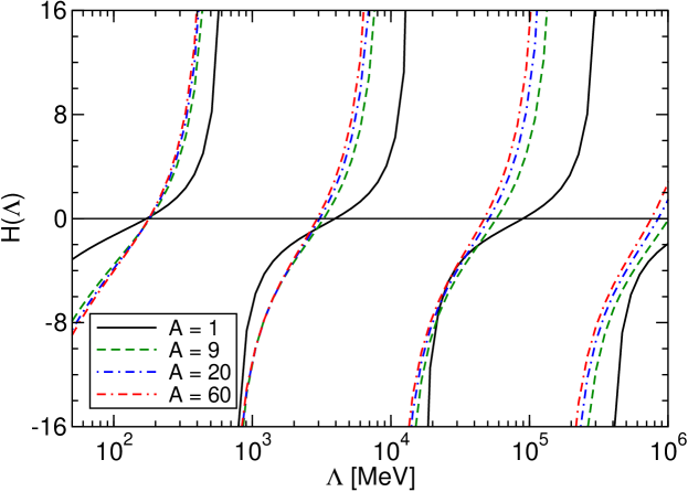
Figure 4: (Color online) The running of $H(\Lambda)$ as a function of the cutoff $\Lambda$ for systems with $A=1$ (solid), $A=9$ (dashed), $A=20$ (dash-dotted), and $A=60$ (dash-dash-dotted). Numerical results are from (Hammer et al., 2017) and obtained for $\gamma_{nn},\gamma_{nc}=0$ and $B_{3}=1$ MeV.

The full three-body wave function $\Psi$ can then be obtained by connecting the three-body transition amplitudes with external one-body propagators and two-body scattering amplitues. The wave function can be represented in two different Jacobi partitions labeled by the spectator $n$ or $c$. In S-wave two-neutron halos, we obtain (Canham and Hammer, 2008; Acharya et al., 2013)

$$\Psi_{n}(p,q) = G_{0}^{c}(p,q;B_{3})\Big{[}\tau_{nc}(q;B_{3})\mathcal{A}_{n}(q)$$ (43)

$$+\frac{1}{2}\int_{-1}^{1}d\left(\hat{\bm{p}}\cdot\hat{\bm{q}}\right)\tau_{nc}(\pi_{3}(\bm{p},-\bm{q});B_{3})\mathcal{A}_{n}(\pi_{3}(\bm{p},-\bm{q}))$$

$$+\frac{1}{2}\int_{-1}^{1}d\left(\hat{\bm{p}}\cdot\hat{\bm{q}}\right)\tau_{nn}(\pi_{1}(\bm{p},-\bm{q});B_{3})\mathcal{A}_{c}(\pi_{1}(\bm{p},-\bm{q}))\Big{]}\,,$$

and with the core as a spectator:

$$\Psi_{c}(p,q) = G_{0}^{n}(p,q;B_{3})\Big{[}\tau_{nn}(q;B_{3})\mathcal{A}_{c}(q)$$ (44)

$$+\int_{-1}^{1}d\left(\hat{\bm{p}}\cdot\hat{\bm{q}}\right)\tau_{nc}(\pi_{2}(\bm{p},-\bm{q});B_{3})\mathcal{A}_{n}(\pi_{2}(\bm{p},-\bm{q}))\big{]}\,.$$

With the wave function, we can calculate the one-body matter-density form factors of an S-wave $2n$ halo. They are defined as

$$F_{y}(|\bm{k}|)=\int d^{3}p\int d^{3}q\,\Psi_{y}(p,q)~{}\Psi_{y}(p,|\bm{q}-\bm{k}|)\,,$$ (45)

with $y=n,c$ depending on the Jacobi partitions. For normalized wave functions $F_{y}(0)=1$ holds automatically. The mean-square distance between the valence neutron and the center of mass of the neutron-core pair, $\langle r^{2}\rangle_{n-nc}$, can be extracted from the form factor $F_{n}$ via

$$F_{n}(|\bm{k}|)=1-\frac{1}{6}\bm{k}^{2}\langle r^{2}\rangle_{n-nc}+\ldots\,,$$ (46)

and the mean-square distance between the core and the center of mass of the two-neutron pair, $\langle r^{2}\rangle_{c-nn}$, is determined by

$$F_{c}(|\bm{k}|)=1-\frac{1}{6}\bm{k}^{2}\langle r^{2}\rangle_{c-nn}+\ldots.$$ (47)

The geometry of the neutron-neutron-core three-body system then leads to the following formula for the total matter radius of a $2n$ halo:

$$\langle r_{m}^{2}\rangle_{2n\rm-halo}=\frac{2(A+1)^{2}}{(A+2)^{3}}\langle r^{2}\rangle_{n-nc}+\frac{4A}{(A+2)^{3}}\langle r^{2}\rangle_{c-nn}+\frac{A}{A+2}\langle r_{m}^{2}\rangle_{\rm core},$$ (48)

where the last term is the correction from the finite matter radius of the core.

4.1 Applications 3: Efimov states and matter radii

In the zero-range limit, long-distance observables in three-body systems are correlated by few-body universality. One example is the Efimov effect discussed in the introduction, which is characterized by discrete scale invariance in the three-body system. In Eq. (41), the running of the three-body coupling, which is a log-periodic function of the ultraviolet cutoff, is characterized by a limit cycle with a period $\exp(\pi/s_{0})$. As a consequence of the limit cycle, the three-body S-wave bound states in the unitary limit display a geometric progression. The ratio of three-body binding energies in two consecutive states is given by $\exp(2\pi/s_{0})$.

Discrete scale invariance has been observed in experiments on ultracold atomic gases, where the atom-atom scattering length is tuned using a magnetic field in the vicinity of a Feshbach resonance. Near the unitary limit, the scattering lengths associated with threshold features in atom-dimer collisions and three-atom recombination are also correlated through the scaling factor $\exp(\pi/s_{0})$, see Braaten and Hammer (2006); Naidon and Endo (2017) for reviews.

In an S-wave $2n$ halo nucleus, $a_{nn}$ and $a_{nc}$ are large but finite, and the three-body binding energy is characterized by the two-neutron separation energy, i.e., $S_{2n}=B_{3}$. In such systems, the number of possible Efimov-like halo states is determined by the two ratios $E_{nn}/S_{2n}$ and $S_{1n}/S_{2n}$, where $E_{nn}=-\gamma_{nn}^{2}/m_{n}$ is the neutron-neutron virtual energy. Amorim et al. (1997) suggested to use a universal function of the ratios $E_{nn}/S_{2n}$ and $S_{1n}/S_{2n}$ to explore possible Efimov states in halo nuclei, and carried out this study in a zero-range three-body model (see also Yamashita et al. (2008)). Following this approach, Canham and Hammer (2008) applied EFT to explore the Efimov scenario in S-wave $2n$ halos. They tuned the three-body coupling $H(\Lambda)$ so that there was an excited state of the two-neutron halo at threshold, i.e. $B_{3}^{*}=\max\{0,E_{nn},S_{1n}\}$. The $S_{2n}$ of the two-neutron halo is then predicted as all LO two-body and three-body EFT couplings are fixed. At this value of $S_{2n}$, LO Halo EFT predicts the existence of an Efimov excited state at threshold in the halo system. This, in turn, defines a contour in the $(S_{1n}/S_{2n})$ versus $(E_{nn}/S_{2n})$ plane:

$$g^{(LO)}\left(\frac{E_{nn}}{S_{2n}},\frac{S_{1n}}{S_{2n}};A\right)=1.$$ (49)

Inside the contour the three-body bound state is deep enough, or the two-body $nc$ system is close enough to unitarity, for an Efimov state to appear in the two-neutron halo. This region is depicted in Fig. 5, and is in good agreement with an analogous study in a zero-range model (Frederico et al., 2012).

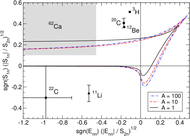
Figure 5: The contour plot in $\textrm{sgn}(E_{nn})\sqrt{|E_{nn}|/S_{2n}}$ versus $\textrm{sgn}(S_{1n})\sqrt{|S_{1n}|/S_{2n}}$ for the ground-state $2n$ halos with core-neutron mass ratios $A=1,10,100$. The hypothetical bound dineutron regime with $E_{nn}>0$ is also included in the theoretical calculation to complete the contour.

The curves depend on the core-neutron mass ratio $A$, but for different values of $A$ quickly converge to an $A$-independent contour when $A$ increases. The specific cases of ³H, ¹¹Li, ¹²Be, ^20,22C and ⁶²Ca are indicated by mapping their experimental data from AME2012 (Audi et al., 2012; Wang et al., 2012) onto this two-dimensional plane (Hammer et al., 2017). Note that Canham and Hammer (2008) originally came to a different conclusion regarding ²⁰C since they relied on older data for $S_{1n}$.

The correlation between bound and excited-state energies is just one example of the way in which universality imposes relations between different three-body observables. The point matter radius $\langle r_{m}^{2}\rangle_{\rm pt}$ of a ground-state two-neutron halo, defined by subtracting the core-size contribution from the radius of the halo in Eq. (48), is also determined by a universal function of $S_{1n}$ and $S_{2n}$ at LO:

$$\langle r_{m}^{2}\rangle_{\rm pt}\equiv\langle r_{m}^{2}\rangle_{2n\rm-halo}-\frac{A}{A+2}\langle r_{m}^{2}\rangle_{\rm core}=\frac{1}{m_{n}S_{2n}}f^{(LO)}\left(\frac{E_{nn}}{S_{2n}},\frac{S_{1n}}{S_{2n}};A\right).$$ (50)

Such correlations have been investigated using EFT for different S-wave two-neutron halos (Canham and Hammer, 2008; Acharya et al., 2013; Hagen et al., 2013).

²²C is a Borromean two-neutron halo. The matter radius of ²²C was determined in the reaction cross section measurement on a proton target to be $\langle r_{m}^{2}\rangle^{1/2}_{2n\rm-halo}=5.4(9)$ fm (Tanaka et al., 2010). A more recent interaction cross-section measurement on a carbon target obtained a more precise result of $\langle r_{m}^{2}\rangle^{1/2}_{2n\rm-halo}=3.44(8)$ fm (Togano et al., 2016), suggesting a smaller halo configuration in ²²C. The $2n$ separation energy of ²²C is not yet directly constrained by experiment. In order to obtain an indirect constraint, Acharya et al. (2013) performed an Halo EFT calculation of the correlations among $\langle r_{m}^{2}\rangle^{1/2}_{2n\rm-halo}$, $S_{1n}$, and $S_{2n}$ of ²²C. Using the value for $\langle r_{m}^{2}\rangle^{1/2}_{2n\rm-halo}$ from Tanaka et al. (2010) known at the time, they predicted an upper bound on $S_{2n}$ of $0.1$ MeV. Hammer et al. (2017) updated this analysis using the more precise value for $\langle r_{m}^{2}\rangle^{1/2}_{2n\rm-halo}$ by Togano et al. (2016) and obtained an upper limit of $S_{2n}\leq 0.4$ MeV in ²²C, suggesting a more deeply bound system.

⁶²Ca, highlighted in Fig. 5 in grey, is predicted to be a $2n$ halo nucleus, but to date has not been observed experimentally. Hagen et al. (2013) extracted the $n$-⁶⁰Ca scattering parameters from the $n$–⁶⁰Ca S-wave scattering phase shift, obtained in an ab initio coupled-cluster calculation based on chiral two- and three-nucleon interactions. The calculation indicated a large scattering length $a_{nc}=54(1)$ fm and an effective range $r_{nc}=9.0(2)$ fm for the $n$-⁶⁰Ca system, where the error is estimated based on the spread of the coupled-cluster calculations at two small harmonic oscillator frequencies. This would make ⁶¹Ca a very shallow ($S_{1n}\approx 7$ keV) one-neutron halo. Using $a_{mc}$ and $r_{nc}$ as input parameters, they performed a Halo EFT analysis on ⁶²Ca as a $n$-$n$-⁶⁰Ca two-neutron halo and searched for possible signatures of Efimov states. The expansion parameter in this system is estimated to be $M_{\rm halo}/M_{\rm core}\sim r_{nc}/a_{nc}=1/6$. They analyzed the LO Halo EFT correlation between the $n$-⁶¹Ca scattering length and the two-neutron separation energy $S_{2n}$ of the ground state of ⁶²Ca. Their conclusion was that for $S_{2n}=230$ keV an excited state of ⁶²Ca appears at the $n$-⁶¹Ca threshold. Thus for $S_{2n}\geq 230$ keV, ⁶²Ca will have an excited bound state of Efimovian character. If confirmed in experiment, this would make ⁶²C the first $2n$ halo with an Efimov excited state and allow for a test of the predicted scaling relation.

4.2 Range corrections in three-body halos

Beyond the leading-order prediction, universal physics in two-neutron halos is affected by the finite effective range which enters EFT calculations at next-to-leading order. There are various approaches to include effective range effects.

The partial resummation technique was developed for studies of range effects for the triton (Bedaque et al., 2003b) and adopted by Canham and Hammer (2010) to investigate range corrections in two-neutron halos. This formalism iterates both the LO and NLO parts of the two-body scattering amplitudes in the three-body integral equations, and thus includes some higher-order range corrections above NLO. These higher-order corrections are small and well-behaved if the cutoff $\Lambda$ is kept below or close to $M_{\rm core}$. See Bedaque et al. (2003b); Platter and Phillips (2006); Ji and Phillips (2013) for detailed discussions of this issue.

An alternative, fully perturbative, EFT calculation of range corrections was recently carried out for two-neutron halos at NLO by Vanasse (2017a). This implemented his rigorous method developed for calculating perturbative range insertions up to N³LO in the three-nucleon system (Vanasse, 2013; Margaryan et al., 2016; Vanasse, 2017b). Results for charge and matter form factors and radii in two neutron halos were obtained with good accuracy. See Vanasse (2017a, b) for a detailed discussion of this approach.

$\langle r_{m}^{2}\rangle_{\rm pt}$ [fm2]	11Li	14Be	22C
EFTLO	$5.76\pm 2.13$	$1.23\pm 0.96$	$8.99^{+\infty}_{-5.01}$
EFTNLO	$6.16\pm 0.84$	$1.40\pm 0.85$	$9.28^{+\infty}_{-5.17}$
expt	$5.34\pm 0.15$	$4.24\pm 2.42$	$21.1\pm 9.7$
		$2.90\pm 2.25$	$3.81^{+0.82}_{-0.71}$

Table 2: The point matter radius, Eq. (50), from EFT predictions by Vanasse (2017a) at LO and NLO. and from experiments. The experimental results for ¹¹Li and ¹⁴Be are from (Ozawa et al., 2001a) while the experimental results for ²²C are from (Ozawa et al., 2001b; Tanaka et al., 2010) (upper row) and  (Togano et al., 2016) (lower row). Compilation taken from (Hammer et al., 2017).

The matter radii in two-neutron halos were calculated to LO in Halo EFT by Canham and Hammer (2008). Using partial resummation, they also predicted the average neutron-core and neutron-neutron distances in the neutron-neutron-core configuration at NLO accuracy (Canham and Hammer, 2010). Vanasse (2017a) calculated the point matter radii, Eq. (50), at NLO accuracy in the perturbative approach. His results are fully consistent with the previous calculations by Canham and Hammer (2008, 2010). In Table 2, we quote Vanasse’s results at LO and NLO and compare with experimental values for ¹¹Li, ¹⁴Be, and ²²C. Note that the NLO numbers were obtained by estimating $r_{nc}\sim 1/M_{\pi}\approx 1.4$ fm. Errors were then determined as $(r_{nc}\sqrt{2m_{n}S_{2n}})^{j}$, where $j=1$ ($j=2$) for the LO (NLO) results shown in the first (second) column.

5 Multi-neutron systems

Due to the large S-wave neutron-neutron scattering length $a_{{}^{1}S_{0}(nn)}=-18.6(5)$ fm and natural effective range $r_{{}^{1}S_{0}(nn)}=2.83(11)$ fm (Chen et al., 2008), which scale as $1/M_{\rm halo}$ and $1/M_{\rm core}$, respectively, multi-neutron systems also show universal halo features. Because $a_{{}^{1}S_{0}(nn)}$ is negative, the dineutron system is unbound as was already discussed above in the context of two-body halos. Here we focus on the universal properties of systems of three and more neutrons. The expansion parameter $M_{\rm halo}/M_{\rm core}\approx 1/7$ is rather favorable in this case. Moreover, three-body interactions are highly suppressed because two of the neutrons have to be in the same spin state and the Pauli principle forbids momentum-independent contact interactions. As a consequence, multi-neutron systems exhibit a higher degree of universality and only two-body information is required as input in the first few orders.

The search for multi-neutron resonances and bound states has a long history (Kezerashvili, 2016). The interest in these systems was revived when experimental evidence for a four-neutron resonance was presented by Kisamori et al. (2016). More recently, Faestermann et al. (2022) reported indications for a bound tetraneutron and various further experimental efforts are under way. An overview of the theoretical and experimental situation can be found in (Marqués and Carbonell, 2021). See also Dietz et al. (2021) for a discussion of the status of three-neutron resonances.

Here, we focus on the universal properties of multi-neutron systems determined by the ERE parameters $a_{{}^{1}S_{0}(nn)}$ and $r_{{}^{1}S_{0}(nn)}$. No further resonant enhancement is assumed. Hammer and Son (2021) showed that such multi-neutron systems display an approximate non-relativistic conformal symmetry or Schrödinger symmetry (Hagen, 1972; Mehen et al., 2000) if their center-of-mass energy $E_{cm}$ is in the range

$$0.1\mbox{ {M}eV}\approx\frac{1}{m_{n}(a_{{}^{1}S_{0}(nn)})^{2}}\ll E_{cm}\ll\frac{1}{m_{n}(r_{{}^{1}S_{0}(nn)})^{2}}\approx 5\mbox{ {M}eV}\,,$$ (51)

and elucidated the consequences of this symmetry for multineutron systems. For neutrons in this energy range, one can safely set $1/a_{{}^{1}S_{0}(nn)}=0$ and $r_{{}^{1}S_{0}(nn)}=0$ at LO in the EFT description, such that no dimensionful interaction parameters are left and the theory is scale invariant. The multi-neutron systems can then be described by a field $\mathcal{U}$ in a non-relativistic conformal field theory (CFT) (Nishida and Son, 2007). In addition to the usual Galilei transformations, the CFT is also invariant under scale transformations

$$\bm{x}\to e^{\lambda}\bm{x},\qquad t\to e^{2\lambda}t\,,$$ (52)

and special conformal transformations

$$\bm{x}\to\frac{\bm{x}}{1+\xi t}\,,\qquad t\to\frac{t}{1+\xi t}\,,$$ (53)

of the space-time variables $\bm{x}$ and $t$, where $\lambda$ and $\xi$ are real parameters.

The full Green’s function of a field $\mathcal{U}$ in CFT is strongly constrained by the conformal symmetry. Up to an overall constant, it depends only on the mass of the field $M_{\mathcal{U}}$ and the scaling dimension $\Delta$, which determines the behavior of the field under scale transformations. Hammer and Son (2021) used this property to derive a general expression for the energy spectra of multi-neutron systems created in high-energy nuclear reactions in terms of $\Delta$. Consider a nuclear reaction of two nuclei $A_{1}$ and $A_{2}$, which produces a few final-state neutrons and a recoil particle $B$,

$$A_{1}+A_{2}\to B+\underbrace{n+n+\cdots}_{N~{}\text{neutrons}}\,.$$ (54)

The number of final-state neutrons $N$ can be $2,3,4,\ldots$. The energy scale of the primary nuclear reaction that produces the neutrons is assumed to be large compared to $E_{cm}$, such that the corresponding matrix element factorizes into two parts: one describing the primary production process which creates the multi-neutron system in a point and one corresponding to the final-state interaction of the neutrons. In the case of two neutrons this provides the basis for the Watson-Migdal approach to final-state interactions (Watson, 1952; Migdal, 1955).

Consider first an experiment where only the energy of the recoil particle $B$ is measured. The inclusive differential cross section as function of the recoil energy $E$ of particle $B$, $d\sigma/dE$, is continuous and vanishes at some maximum recoil energy $E_{0}$. Near the end point, where the neutrons satisfy Eq. (51), it has the general form

$$\frac{d\sigma}{dE}\sim(E_{0}-E)^{\Delta-\frac{5}{2}}\,.$$ (55)

If the low-energy spectrum $P(E_{cm})$ of the multineutron system in its center-of-mass itself is measured, it takes the form

$$P(E_{cm})\sim(E_{cm})^{\Delta-\frac{5}{2}}\,.$$ (56)

Thus the energy spectra for $E_{cm}$ in the kinematical range given by Eq. (51) follow a universal power law that is determined by the scaling dimension of the $N$-neutron system. For very small energies $\sqrt{m_{n}E_{cm}}\ll 1/a_{{}^{1}S_{0}(nn)}$, the neutrons show free particle behavior. The transition to the conformal window can be calculated in pionless EFT.

The scaling dimension $\Delta$ for a free neutron is $3/2$, for $N$ free neutrons it is $3N/2$. For a system of interacting neutrons $\Delta$ can be obtained from a field theory calculation (cf. Braaten and Hammer (2021)) or from the energy of the corresponding few-neutron system in the unitary limit placed in a harmonic potential with unit oscillator frequency (Nishida and Son, 2007). This so-called operator state correspondence leads to an nontrivial connection between the few-body physics of spin-1/2 fermions at unitarity and the physics of nuclear reactions. Namely, the spectrum of spin-1/2 fermions at unitarity in a harmonic trap determines the behavior of the processes involving emission of neutrons in a certain kinematic regime. The lowest scaling dimensions for some $N$-neutron systems are collected in Table 3.

$N$	$S$	$L$	$\Delta$
2	0	0	2
3	1/2	0	4.66622
3	1/2	1	4.27272
4	0	0	5.07(1)
5	1/2	1	7.6(1)
6	0	0	8.67(3)

Table 3: Scaling dimensions $\Delta$ for $N$-neutron systems with spin $S$ and orbital angular momentum $L$ in the unitary limit. Numbers taken from (Nishida and Son, 2007).

Hammer and Son (2021) demonstrated that the two- and three-neutron spectra of state-of-the-art calculations for the reactions ⁶He$(p,p\alpha)2n$ (Göbel et al., 2021), ³H$(\pi^{-},\gamma)3n$ (Golak et al., 2018), and ³H$(\mu^{-},\nu_{\mu})3n$ (Golak et al., 2016) exhibit the universal power law behavior. Moreover, the power law is consistent with the experimental photon spectrum near the kinematical end point for radiative capture of stopped pions on tritium measured by Miller et al. (1980). A stringent test of the prediction, Eq. (56), may become possible in current experiments searching for tetraneutron resonances which will produce precise four-neutron spectra at low energies.

6 Further reading

In this chapter, we have provided an introduction to the description of two and three-body halo systems using Halo EFT. Due to space constraints, the focus has been on systems dominated by S-wave neutron-core interactions and their universal structural properties.

Halo EFT and universality has a much wider range of applications, including systems with higher partial wave interactions and/or strangeness, proton halos and systems with Coulomb repulsion, as well as electroweak currents and reactions. For a detailed discussion of these issues, we refer the reader to the reviews by Rupak (2016); Hammer et al. (2017, 2020). An application of Halo EFT to describe nuclear reactions was recently developed by Capel et al. (2018); Moschini et al. (2019); Capel et al. (2021).

For the description of the properties and reactions of halo nuclei using similar and complementary methods, we refer the reader to the excellent reviews on this topic Zhukov et al. (1993); Nielsen et al. (2001); Jensen et al. (2004); Ogata and Bertulani (2010); Baye and Capel (2012); Pfutzner et al. (2012); Frederico et al. (2012); Canto et al. (2015); Moro (2019).

We thank Chen Ji and Daniel R. Phillips for a fruitful collaboration that led to this chapter and Chen Ji for comments on the manuscript. This work was supported in part by the Deutsche Forschungsgemeinschaft (DFG, German Research Foundation) – Projektnummer 279384907 – SFB 1245 and by the German Federal Ministry of Education and Research (BMBF) (Grant No. 05P21RDFNB).

References

- Acharya et al. (2013) Acharya, B., C. Ji, and D. R. Phillips (2013), Phys. Lett. B 723, 196.
- Acharya and Phillips (2013) Acharya, B., and D. R. Phillips (2013), Nucl. Phys. A 913, 103.
- Afnan and Thomas (1977) Afnan, I. R., and A. W. Thomas (1977), Top. Curr. Phys. 2, 1.
- Ajzenberg-Selove (1987) Ajzenberg-Selove, F. (1987), Nucl. Phys. A 475, 1.
- Ajzenberg-Selove (1991) Ajzenberg-Selove, F. (1991), Nucl. Phys. A 523, 1.
- Albeverio et al. (1981) Albeverio, S., R. Hoegh-Krohn, and T. T. Wu (1981), Phys. Lett. A 83, 105.
- Amorim et al. (1997) Amorim, A. E. A., T. Frederico, and L. Tomio (1997), Phys. Rev. C 56, R2378.
- Audi et al. (2012) Audi, G., M. Wang, A. Wapstra, F. Kondev, M. MacCormick, X. Xu, and B. Pfeiffer (2012), Chinese Physics C 36, 1287.
- Barford and Birse (2005) Barford, T., and M. C. Birse (2005), J. Phys. A 38, 697.
- Baye and Capel (2012) Baye, D., and P. Capel (2012), Lect. Notes Phys. 848, 121.
- Baye and Descouvemont (1985) Baye, D., and P. Descouvemont (1985), Annals Phys. (NY) 165, 115.
- Beane et al. (1998) Beane, S. R., T. D. Cohen, and D. R. Phillips (1998), Nucl. Phys. A 632, 445.
- Bedaque et al. (1999a) Bedaque, P. F., H.-W. Hammer, and U. van Kolck (1999a), Phys. Rev. Lett. 82, 463.
- Bedaque et al. (1999b) Bedaque, P. F., H.-W. Hammer, and U. van Kolck (1999b), Nucl. Phys. A 646, 444.
- Bedaque et al. (2003a) Bedaque, P. F., H.-W. Hammer, and U. van Kolck (2003a), Phys. Lett. B 569, 159.
- Bedaque and van Kolck (2002) Bedaque, P. F., and U. van Kolck (2002), Ann. Rev. Nucl. Part. Sci. 52, 339.
- Bedaque et al. (2003b) Bedaque, P. F., G. Rupak, H. W. Griesshammer, and H.-W. Hammer (2003b), Nucl. Phys. A 714, 589.
- Bertulani et al. (2002) Bertulani, C. A., H.-W. Hammer, and U. Van Kolck (2002), Nucl. Phys. A 712, 37.
- Braaten et al. (2012) Braaten, E., P. Hagen, H.-W. Hammer, and L. Platter (2012), Phys. Rev. A 86, 012711.
- Braaten and Hammer (2006) Braaten, E., and H.-W. Hammer (2006), Phys. Rept. 428, 259.
- Braaten and Hammer (2007) Braaten, E., and H.-W. Hammer (2007), Annals Phys. 322, 120.
- Braaten and Hammer (2021) Braaten, E., and H.-W. Hammer (2021), Phys. Rev. Lett. (in press) arXiv:2107.02831 [hep-ph] .
- Braun et al. (2019) Braun, J., W. Elkamhawy, R. Roth, and H.-W. Hammer (2019), J. Phys. G 46, 115101.
- Calci et al. (2016) Calci, A., P. Navrátil, R. Roth, J. Dohet-Eraly, S. Quaglioni, and G. Hupin (2016), Phys. Rev. Lett. 117, 242501.
- Canham and Hammer (2008) Canham, D. L., and H.-W. Hammer (2008), Eur. Phys. J. A 37, 367.
- Canham and Hammer (2010) Canham, D. L., and H.-W. Hammer (2010), Nucl. Phys. A 836, 275.
- Canto et al. (2015) Canto, L. F., P. R. S. Gomes, R. Donangelo, J. Lubian, and M. S. Hussein (2015), Phys. Rept. 596, 1.
- Capel et al. (2018) Capel, P., D. R. Phillips, and H.-W. Hammer (2018), Phys. Rev. C 98, 034610.
- Capel et al. (2021) Capel, P., D. R. Phillips, and H.-W. Hammer (2021), Phys. Lett. B 825, 136847.
- Chen et al. (1999) Chen, J.-W., G. Rupak, and M. J. Savage (1999), Nucl. Phys. A 653, 386.
- Chen et al. (2008) Chen, Q., et al. (2008), Phys. Rev. C 77, 054002.
- Dietz et al. (2021) Dietz, S., H.-W. Hammer, S. König, and A. Schwenk (2021), arXiv:2109.11356 [nucl-th] .
- Efimov (1970) Efimov, V. (1970), Phys. Lett. B 33, 563.
- Efimov (1971) Efimov, V. (1971), Sov. J. Nucl. Phys. 12, 589.
- Efimov (1979) Efimov, V. (1979), Sov. J. Nucl. Phys. 29, 546.
- Epelbaum et al. (2009) Epelbaum, E., H.-W. Hammer, and U.-G. Meißner (2009), Rev. Mod. Phys. 81, 1773.
- Faddeev (1961) Faddeev, L. D. (1961), Sov. Phys. JETP 12, 1014, [Zh. Eksp. Teor. Fiz. 39, 1459 (1960)].
- Faestermann et al. (2022) Faestermann, T., A. Bergmaier, R. Gernhäuser, D. Koll, and M. Mahgoub (2022), Phys. Lett. B 824, 136799.
- Fernando et al. (2015) Fernando, L., A. Vaghani, and G. Rupak (2015), arXiv:1511.04054 [nucl-th] .
- Frederico et al. (2012) Frederico, T., A. Delfino, L. Tomio, and M. T. Yamashita (2012), Prog. Part. Nucl. Phys. 67, 939.
- Freer (2007) Freer, M. (2007), Rep. Prog. Phys. 70, 2149.
- Friar et al. (1997) Friar, J. L., J. Martorell, and D. W. L. Sprung (1997), Phys. Rev. A 56, 4579.
- Furnstahl et al. (2015) Furnstahl, R. J., N. Klco, D. R. Phillips, and S. Wesolowski (2015), Phys. Rev. C 92, 024005.
- Gardestig (2009) Gardestig, A. (2009), J. Phys. G 36, 053001.
- Glöckle (1983) Glöckle, W. (1983), The Quantum Mechanical Few-Body Problem (Springer, Berlin, Heidelberg).
- Göbel et al. (2021) Göbel, M., T. Aumann, C. A. Bertulani, T. Frederico, H.-W. Hammer, and D. R. Phillips (2021), Phys. Rev. C 104, 024001.
- Golak et al. (2018) Golak, J., R. Skibiński, K. Topolnicki, H. Witała, A. Grassi, H. Kamada, A. Nogga, and L. E. Marcucci (2018), Phys. Rev. C 98, 054001.
- Golak et al. (2016) Golak, J., R. Skibiński, H. Witała, K. Topolnicki, H. Kamada, A. Nogga, and L. E. Marcucci (2016), Phys. Rev. C 94, 034002.
- Greene et al. (2017) Greene, C. H., P. Giannakeas, and J. Perez-Rios (2017), Rev. Mod. Phys. 89, 035006.
- Guo et al. (2018) Guo, F.-K., C. Hanhart, U.-G. Meißner, Q. Wang, Q. Zhao, and B.-S. Zou (2018), Rev. Mod. Phys. 90, 015004.
- Hackenburg (2006) Hackenburg, R. W. (2006), Phys. Rev. C 73, 044002.
- Hafstad and Teller (1938) Hafstad, L. R., and E. Teller (1938), Phys. Rev. 54, 681.
- Hagen (1972) Hagen, C. R. (1972), Phys. Rev. D 5, 377.
- Hagen et al. (2013) Hagen, G., P. Hagen, H.-W. Hammer, and L. Platter (2013), Phys. Rev. Lett. 111, 132501.
- Hammer et al. (2017) Hammer, H.-W., C. Ji, and D. R. Phillips (2017), J. Phys. G 44, 103002.
- Hammer et al. (2020) Hammer, H.-W., S. König, and U. van Kolck (2020), Rev. Mod. Phys. 92, 025004.
- Hammer and Lee (2010) Hammer, H.-W., and D. Lee (2010), Annals Phys. 325, 2212.
- Hammer and Phillips (2011) Hammer, H.-W., and D. R. Phillips (2011), Nucl. Phys. A 865, 17.
- Hammer and Platter (2010) Hammer, H.-W., and L. Platter (2010), Ann. Rev. Nucl. Part. Sci. 60, 207.
- Hammer and Son (2021) Hammer, H.-W., and D. T. Son (2021), Proc. Nat. Acad. Sci. 118, e2108716118.
- Hansen et al. (1995) Hansen, P. G., A. S. Jensen, and B. Jonson (1995), Ann. Rev. Nucl. Part. Sci. 45, 591.
- Hansen and Jonson (1987) Hansen, P. G., and B. Jonson (1987), Europhys. Lett. 4, 409.
- Harada et al. (2009) Harada, K., H. Kubo, and A. Ninomiya (2009), Int. J. Mod. Phys. A 24, 3191.
- Herrmann and Rosenfelder (1998) Herrmann, T., and R. Rosenfelder (1998), Eur. Phys. J. A 2, 28.
- Horiuchi and Ikeda (1986) Horiuchi, H., and K. Ikeda (1986), Int. Rev. Nucl. Phys. 4, 1.
- Ikeda et al. (1968) Ikeda, K., N. Takigawa, and H. Horiuchi (1968), Prog. Theo. Phys. Supp. E68, 464.
- Jensen et al. (2004) Jensen, A. S., K. Riisager, D. V. Fedorov, and E. Garrido (2004), Rev. Mod. Phys. 76, 215.
- Ji and Phillips (2013) Ji, C., and D. R. Phillips (2013), Few Body Syst. 54, 2317.
- Jonson (2004) Jonson, B. (2004), Physics Reports 389, 1 .
- Kanungo et al. (2016) Kanungo, R., et al. (2016), Phys. Rev. Lett. 117, 102501.
- Kaplan (1995) Kaplan, D. B. (1995), in 7th Summer School in Nuclear Physics Symmetries, arXiv:nucl-th/9506035 .
- Kaplan (2005) Kaplan, D. B. (2005), arXiv:nucl-th/0510023 .
- Kaplan et al. (1998) Kaplan, D. B., M. J. Savage, and M. B. Wise (1998), Phys. Lett. B 424, 390.
- Kezerashvili (2016) Kezerashvili, R. Y. (2016), in 6th International Conference on Fission and Properties of Neutron Rich Nuclei, arXiv:1608.00169 [nucl-th] .
- Kisamori et al. (2016) Kisamori, K., S. Shimoura, H. Miya, S. Michimasa, S. Ota, M. Assie, H. Baba, T. Baba, D. Beaumel, M. Dozono, et al. (2016), Phys. Rev. Lett. 116, 052501.
- Kobayashi et al. (2012) Kobayashi, N., et al. (2012), Phys. Rev. C 86, 054604.
- van Kolck (1999) van Kolck, U. (1999), Nucl. Phys. A 645, 273.
- König et al. (2017) König, S., H. W. Grießhammer, H.-W. Hammer, and U. van Kolck (2017), Phys. Rev. Lett. 118, 202501.
- Langevin et al. (1985) Langevin, M., et al. (1985), Phys. Lett. B 150, 71.
- Macchiavelli (2015) Macchiavelli, A. O. (2015), Proceedings, Critical Stability 2014: Santos, Brazil, October 12-17, 2014, Few Body Syst. 56, 773.
- Maddalena et al. (2001) Maddalena, V., et al. (2001), Phys. Rev. C 63, 024613.
- Margaryan et al. (2016) Margaryan, A., R. P. Springer, and J. Vanasse (2016), Phys. Rev. C 93 (5), 054001.
- Marqués and Carbonell (2021) Marqués, F. M., and J. Carbonell (2021), Eur. Phys. J. A 57, 105.
- Mehen et al. (2000) Mehen, T., I. W. Stewart, and M. B. Wise (2000), Phys. Lett. B 474, 145.
- Migdal (1955) Migdal, A. B. (1955), Sov. Phys. JETP 1, 2.
- Miller et al. (1980) Miller, J. P., et al. (1980), Nucl. Phys. A 343, 347.
- Mohr et al. (2006) Mohr, R. F., R. J. Furnstahl, R. J. Perry, K. G. Wilson, and H.-W. Hammer (2006), Annals Phys. 321, 225.
- Moro (2019) Moro, A. M. (2019), Proc. Int. Sch. Phys. Fermi 201, 129.
- Mosby et al. (2013) Mosby, S., et al. (2013), Nucl. Phys. A 909, 69.
- Moschini et al. (2019) Moschini, L., J. Yang, and P. Capel (2019), Phys. Rev. C 100, 044615.
- Naidon and Endo (2017) Naidon, P., and S. Endo (2017), Rept. Prog. Phys. 80, 056001.
- Nakamura et al. (1999) Nakamura, T., et al. (1999), Phys. Rev. Lett. 83, 1112.
- Nakamura et al. (2003) Nakamura, T., et al. (2003), Physics of unstable nuclei. Proceedings, International Symposium, ISPUN’02, Halong Bay, Vietnam, November 20-25, 2002, Nucl. Phys. A 722, C301.
- Nakamura et al. (2009) Nakamura, T., et al. (2009), Phys. Rev. C 79, 035805.
- Nielsen et al. (2001) Nielsen, E., D. Fedorov, A. Jensen, and E. Garrido (2001), Phys. Rep. 347, 373 .
- Nishida (2012) Nishida, Y. (2012), Phys. Rev. A 86, 012710.
- Nishida and Son (2007) Nishida, Y., and D. T. Son (2007), Phys. Rev. D 76, 086004.
- Ogata and Bertulani (2010) Ogata, K., and C. A. Bertulani (2010), Prog. Theor. Phys. 123, 701.
- Ozawa et al. (2001a) Ozawa, A., T. Suzuki, and I. Tanihata (2001a), Nucl. Phys. A 693, 32.
- Ozawa et al. (2001b) Ozawa, A., et al. (2001b), Nucl. Phys. A 691, 599.
- Pfutzner et al. (2012) Pfutzner, M., M. Karny, L. V. Grigorenko, and K. Riisager (2012), Rev. Mod. Phys. 84, 567.
- Phillips (1968) Phillips, A. (1968), Nucl. Phys. A 107, 209.
- Phillips and Cohen (1997) Phillips, D. R., and T. D. Cohen (1997), Phys. Lett. B 390, 7.
- Phillips et al. (2000) Phillips, D. R., G. Rupak, and M. J. Savage (2000), Phys. Lett. B 473, 209.
- Platter et al. (2004) Platter, L., H.-W. Hammer, and U.-G. Meißner (2004), Phys. Rev. A 70, 052101.
- Platter and Phillips (2006) Platter, L., and D. R. Phillips (2006), Few Body Syst. 40, 35.
- Riisager (2013) Riisager, K. (2013), Phys. Scripta T152, 014001.
- Rupak (2016) Rupak, G. (2016), Int. J. Mod. Phys. E 25, 1641004.
- Rupak et al. (2012) Rupak, G., L. Fernando, and A. Vaghani (2012), Phys. Rev. C 86, 044608.
- Smith et al. (2015) Smith, J. K., et al. (2015), Nucl. Phys. A 940, 235.
- Tanaka et al. (2010) Tanaka, K., et al. (2010), Phys. Rev. Lett. 104, 062701.
- Tanihata (2016) Tanihata, I. (2016), Eur. Phys. J. Plus 131, 90.
- Tanihata et al. (2013) Tanihata, I., H. Savajols, and R. Kanungo (2013), Prog. Part. Nucl. Phys. 68, 215.
- Tanihata et al. (1985) Tanihata, I., et al. (1985), Phys. Rev. Lett. 55, 2676.
- Tilley et al. (2004) Tilley, D. R., et al. (2004), Nucl. Phys. A 745, 155.
- Togano et al. (2016) Togano, Y., et al. (2016), Phys. Lett. B 761, 412.
- Vanasse (2013) Vanasse, J. (2013), Phys. Rev. C 88, 044001.
- Vanasse (2017a) Vanasse, J. (2017a), Phys. Rev. C 95, 024318.
- Vanasse (2017b) Vanasse, J. (2017b), Phys. Rev. C 95, 024002.
- Wang et al. (2012) Wang, M., G. Audi, A. Wapstra, F. Kondev, M. MacCormick, X. Xu, and B. Pfeiffer (2012), Chinese Physics C 36, 1603.
- Watson (1952) Watson, K. M. (1952), Phys. Rev. 88, 1163.
- Wilson (1971) Wilson, K. G. (1971), Phys. Rev. D 3, 1818.
- Yamashita et al. (2008) Yamashita, M. T., T. Frederico, and L. Tomio (2008), Phys. Lett. B 660, 339.
- Zhukov et al. (1993) Zhukov, M. V., B. V. Danilin, D. V. Fedorov, J. M. Bang, I. J. Thompson, and J. S. Vaagen (1993), Phys. Rept. 231, 151.