Inner and Outer Approximations of Star-Convex Semialgebraic Sets

Abstract

We consider the problem of approximating a semialgebraic set with a sublevel-set of a polynomial function. In this setting, it is standard to seek a minimum volume outer approximation and/or maximum volume inner approximation. As there is no known relationship between the coefficients of an arbitrary polynomial and the volume of its sublevel sets, previous works have proposed heuristics based on the determinant and trace objectives commonly used in ellipsoidal fitting. For the case of star-convex semialgebraic sets, we propose a novel objective which yields both an outer and an inner approximation while minimizing the ratio of their respective volumes. This objective is scale-invariant and easily interpreted. Numerical examples demonstrate that the approximations obtained are often tighter than those returned by existing heuristics. We also provide methods for establishing the star-convexity of a semialgebraic set by finding inner and outer approximations of its kernel.

I INTRODUCTION

Consider a compact, semialgebraic set $\mathcal{X}\subset\mathbb{R}^{n}$ given by the intersection of the 1-sublevel sets of $m$ polynomial functions $g_{i}(x)\in\mathbb{R}[x]$:

$$\mathcal{X}=\{x\,|\,g_{i}(x)\leq 1,\,i\in[m]\}.$$ (1)

Semialgebraic sets arise naturally in many control applications. The set of coefficients for which a polynomial is Schur or Hurwitz stable is given by a semialgebraic set. For Hurwitz stability, the polynomial inequalities can be derived from the Routh array. These sets are often complicated and cumbersome to analyze. As such, it is common to seek simpler representations which closely approximate the set but are more amenable to further analysis [1]. Examples of “simple” representations include hyperrectangles and ellipsoids.

A number of publications have explored the use of sum-of-squares (SOS) optimization for approximating a semialgebraic set with a simpler representation [1, 2, 3, 4, 5, 6, 7, 8]. The most common parameterization is to seek a SOS polynomial whose 1-sublevel set $\mathcal{F}=\{x\,|\,f(x)\leq 1\}$ provides either an inner ($\mathcal{F}\subseteq\mathcal{X}$) or outer ($\mathcal{F}\supseteq\mathcal{X}$) approximation of the set $\mathcal{X}$.

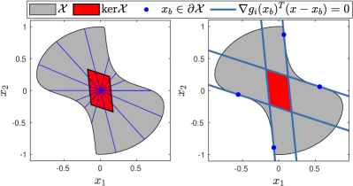
Figure 1: The kernel is the convex set of points $p\in\mathcal{X}$ such that the line segment $\overline{pq}\subseteq\mathcal{X}$ for any $q\in\mathcal{X}$ (left). It is given by the intersection of all linearized active constraints $g_{i}(x_{b})=1$ defining $\partial\mathcal{X}$ (right).

In this formulation, an open question is the choice of the objective function. For outer (resp. inner) approximations, a natural objective is to minimize (resp. maximize) the volume of the 1-sublevel set. For an ellipsoid $\mathcal{E}=\{x\,|\,x^{T}Ax+b^{T}x+c\leq 1\}$ where $A\succeq 0$, the volume is proportional to $\textup{det}A^{-1}$. Using the logarithmic transform, ellipsoidal volume minimization can be posed as the convex objective $-\textup{logdet}A$ [2]. More generally, in the case of homogeneous polynomials it is possible to find the minimum volume outer approximation by solving a hierarchy of semidefinite programs [9].

Ellipsoids and homogeneous polynomials are not ideal candidates for approximating asymmetric shapes due to their inherent symmetry. General polynomials offer a more flexible basis for approximating sets. The caveat is that we lack expressions for computing the volume of the 1-sublevel set as a function of the polynomial coefficients. The most common approach is to mimic the determinant ([2, 4]) or trace [1] objectives used in ellipsoidal fitting. These objectives often yield qualitatively good approximations. However, they have no explicit relationship to the volume beyond upper bounding it in some cases [1]. Thus it is difficult to infer the quality of an approximation from the objective value attained.

I-A Contributions

This paper makes the following contributions:

• We propose and justify an algorithm based on SOS optimization for jointly finding an inner and outer approximation of a semialgebraic set. The algorithm minimizes the volume of the outer approximation relative to the volume of the inner approximation. This objective is easily interpreted and scale-invariant.

• We provide numerical examples showing that our algorithm tends to yield better approximations than existing methods when applied to star-convex sets.

• We provide algorithms for finding inner and outer approximations of the kernel of a star-convex set as shown in Figure 1.

The paper is organized as follows. Section II defines the problem we address and reviews the notion of star-convexity. Section III surveys existing volume heuristics for SOS-based set approximation. Section IV proposes a new volume heuristic for finding outer and inner approximations. Section V provides methods for approximating the kernel of a star-convex set. Section VI provides numerical examples. Section VII concludes the paper.

I-B Notation

Let $i\in[k]\mathrel{\mathop{\mathchar 58\relax}}=\{1,\ldots,k\}$. Let $\mathbb{Z}^{+}$ denote the set of positive integers. Let $S^{n-1}\mathrel{\mathop{\mathchar 58\relax}}=\{x\in\mathbb{R}^{n}\,|\,\|x\|=1\}$. The notation $P\succeq 0$ indicates that the symmetric matrix $P$ is positive semidefinite (PSD). Given a compact set $\mathcal{X}\subset\mathbb{R}^{n}$, its volume (formally, Lebesgue measure) is denoted $\textup{vol }\mathcal{X}\mathrel{\mathop{\mathchar 58\relax}}=\int_{\mathcal{X}}dx$. Let $\sigma_{\mathcal{X}}(c)\mathrel{\mathop{\mathchar 58\relax}}=\underset{x\in\mathcal{X}}{\textup{max}}\,c^{T}x$ denote the support function of $\mathcal{X}$ where $c\in S^{n-1}$. Given sets $\mathcal{A},\mathcal{B}\subseteq\mathbb{R}^{n}$ the (bi-directional) Hausdorff distance is $d_{H}(\mathcal{A},\mathcal{B})\mathrel{\mathop{\mathchar 58\relax}}=\textup{max}(h(\mathcal{A},\mathcal{B}),h(\mathcal{B},\mathcal{A}))$ where $h(\mathcal{A},\mathcal{B})\mathrel{\mathop{\mathchar 58\relax}}=\underset{a\in\mathcal{A}}{\textup{max}}\,\underset{b\in\mathcal{B}}{\textup{min}}\,\|a-b\|_{2}$.

The $\alpha$-sublevel set of a function $f(x)\mathrel{\mathop{\mathchar 58\relax}}\mathbb{R}^{n}\rightarrow\mathbb{R}$ is $\{x\in\mathbb{R}^{n}\,|\,f(x)\leq\alpha\}$. For $x\in\mathbb{R}^{n}$, let $\mathbb{R}[x]$ denote the set of polynomials in $x$ with real coefficients. Let $\mathbb{R}_{d}[x]$ denote the set of all polynomials in $\mathbb{R}[x]$ of degree less than or equal to $d$. A polynomial $p(x)\in\mathbb{R}[x]$ is a SOS polynomial if there exists polynomials $q_{i}(x)\in\mathbb{R}[x],i\in[j]$ such that $p(x)=q_{1}^{2}(x)+\ldots+q_{j}^{2}(x)$. We use $\Sigma[x]$ to denote the set of SOS polynomials in $x$. A polynomial of degree $2d$ is a SOS polynomial if and only if there exists $P\succeq 0$ (the Gram matrix) such that $p(x)=z(x)^{T}Pz(x)$ where $z(x)$ is the vector of all monomials of $x$ up to degree $d$ [10]. Letting $m\mathrel{\mathop{\mathchar 58\relax}}=\binom{n+d}{d}$ denote the length of $z(x)$, we have that $P\in\mathbb{R}^{m\times m}$. To minimize notational clutter, we will sometimes list a polynomial $f(x)$ as a decision variable. It is implied that a degree is specified and matrix $P$ is introduced as a decision variable such that $f(x)=z(x)^{T}Pz(x)$.

II Problem Statement

Definition 1 (Star-Convex Set [11]).

A set $\mathcal{S}\subseteq\mathbb{R}^{n}$ is star-convex if it has a non-empty kernel. The kernel is

$$\textup{ker}\;\mathcal{S}\mathrel{\mathop{\mathchar 58\relax}}=\{x\,|\,tx+(1-t)y\in\mathcal{S}\,\forall\,t\in[0,1],y\in\mathcal{S}\}.$$ (2)

The kernel is the set of points in $\mathcal{S}$ from which one can “see” all of $\mathcal{S}$ as shown in Figure 1. It is easily shown that the kernel is convex. If $\mathcal{S}$ is convex then $\textup{ker}\,\mathcal{S}=\mathcal{S}$.

We will be interested in approximating the set (1) for the case in which it is star-convex with respect to the origin.

Problem 1 (Star-Convex Set Approximation).

Given a compact, semialgebraic set $\mathcal{X}$ with $0\in\textup{int}\mathcal{X}\cap\textup{ker}\mathcal{X}$ and $d\in\mathbb{Z}^{+}$ find a polynomial $f_{o}(x)\in\mathbb{R}_{2d}[x]$ ($f_{i}(x)\in\mathbb{R}_{2d}[x]$) whose 1-sublevel set $\mathcal{F}_{o}$ ($\mathcal{F}_{i}$) is of minimum (maximum) volume and is an outer (inner) approximation of $\mathcal{X}$:

$$\underset{f_{o}(x)\in\mathbb{R}_{2d}[x]}{\textup{min}}\textup{ vol }\mathcal{F}_{o}\textup{ s.t. }\mathcal{X}\subseteq\mathcal{F}_{o}$$

$$\left(\underset{f_{i}(x)\in\mathbb{R}_{2d}[x]}{\textup{max}}\textup{ vol }\mathcal{F}_{i}\textup{ s.t. }\mathcal{F}_{i}\subseteq\mathcal{X}\right).$$

To establish star-convexity of $\mathcal{X}$, we seek polytopic approximations of its kernel.

Problem 2 (Kernel Approximation).

Given a semialgebraic set $\mathcal{X}\subset\mathbb{R}^{n}$ find a polytope $\mathcal{K}_{o}$ ($\mathcal{K}_{i}$) of minimum (maximum) volume that is an outer (inner) approximation of $\textup{ker}\mathcal{X}$:

$$\textup{min vol }\mathcal{K}_{o}\textup{ s.t. }\textup{ker}\mathcal{X}\subseteq\mathcal{K}_{o}$$

$$\left(\textup{max vol }\mathcal{K}_{i}\textup{ s.t. }\mathcal{K}_{i}\subseteq\textup{ker}\mathcal{X}\right).$$

III Existing Volume Heuristics for Set Approximation

We review existing heuristics for approximating semialgebraic set $\mathcal{X}$ using SOS optimization. Each of these methods finds an even-degree polynomial $f(x)=z(x)^{T}Pz(x)$. The variations between the methods largely relate to the objective applied to Gram matrix $P$. For general polynomials, there is no known relationship between $P$ and the volume of the sublevel sets. Thus the following objectives are all heuristics in some sense.

III-A Determinant Maximization $(-\textup{det}P)$

In [2], the authors propose maximizing the determinant of the Hessian $\nabla^{2}f(x)$ of SOS polynomials. If $f$ is a polynomial of degree 2, this reduces to the ellipsoidal objective $-\textup{det}A$ for $\mathcal{E}=\{x\,|\,x^{T}Ax+b^{T}x+c\leq 1\},A\succeq 0$. As the Hessian must be PSD, the outer approximation is convex. This makes it ill-suited to approximating non-convex shapes.

In [4], the authors propose performing determinant maximization directly on the Gram matrix $P$. The Hessian is no longer required to be PSD. This allows non-convex outer approximations to be found.

III-B Inverse Trace Minimization $(\textup{tr}P^{-1})$

The determinant maximization objective minimizes the product of the eigenvalues of $P^{-1}$. In [4], the authors propose an alternative heuristic of minimizing the sum of the eigenvalues of $P^{-1}$. This requires an additional matrix variable $V$ and constraint $V\succeq P^{-1}$. Using the Schur complement this can be written as a block matrix constraint involving $V$ and $P$ (vice $P^{-1}$). The objective $\textup{min tr}V$ then indirectly minimizes the sum of the eigenvalues of $P^{-1}$.

III-C $l_{1}$ Minimization

In [1] the authors propose minimizing the $l_{1}$ norm of a polynomial evaluated over a bounding box $\mathcal{B}\supseteq\mathcal{X}$. This approach was first introduced in [12] for approximating the volume of semialgebraic sets. Using hyperrectangles as bounding boxes, one can integrate the polynomial over $\mathcal{B}$. The resulting objective $l_{1}(f(x))\mathrel{\mathop{\mathchar 58\relax}}=\int_{\mathcal{B}}f(x)\,dx$ is linear in terms of $P$. The outer approximation consists of the intersection of the 1-superlevel set of $f(x)$ and $\mathcal{B}$:

$$\mathcal{X}\subseteq(\mathcal{B}\cap\{x\,|\,f(x)\geq 1\}).$$ (3)

This differs from other objectives which do not rely on bounding boxes as part of the set approximation. In this setting, $f(x)$ is approximating the indicator function of $\mathcal{X}$ over a compact set $\mathcal{B}$. Convergence of $f(x)$ to the true indicator function in the limit (as degree $d\rightarrow\infty$) can be shown by leveraging the Stone-Weierstrass theorem. The asymptotic rate of convergence is at least $O(1/\textup{log log }d)$ [13]. Inner approximations can be found by outer approximating the complement of $\mathcal{X}$.

IV Inner and Outer Approximations of Star-Convex Sets

We propose a new volume heuristic for solving Problem 1. Our heuristic is inspired by the following two lemmas.

Lemma 1.

Let $\mathcal{X},\mathcal{F}$ be compact sets in $\mathbb{R}^{n}$ such that $\mathcal{F}\subseteq\mathcal{X}$. Let $0\in\textup{int }\mathcal{F}$. Then there exists a scaling $s\geq 1$ such that $\mathcal{X}\subseteq s\mathcal{F}$.

Lemma 2.

Let $\mathcal{X}\subset\mathbb{R}^{n}$. Let $s\mathcal{X}=\{sx\,|\,x\in\mathcal{X}\}$ denote the scaled set where $s\geq 0$. Then $\textup{vol }s\mathcal{X}=s^{n}\cdot\textup{vol}\mathcal{X}$.

Thus given an inner approximation $\mathcal{F}$, we can obtain an outer approximation $s\mathcal{F}$ for some $s\geq 1$ with relation

$$\frac{\textup{vol }s\mathcal{F}}{\textup{vol }\mathcal{F}}=s^{n}.$$ (4)

By minimizing $s$ we minimize the ratio of the outer approximation volume to the inner approximation volume. Figure 2 visualizes this intuitive heuristic for approximating a set.

We seek a polynomial $f\mathrel{\mathop{\mathchar 58\relax}}\mathbb{R}^{n}\rightarrow\mathbb{R}$ whose 1-sublevel set $\mathcal{F}=\{x\,|\,f(x)\leq 1\}$ is an inner approximation of $\mathcal{X}$. We turn this into a condition involving the complement of $\mathcal{X}$:

$$\mathcal{F}\subseteq\mathcal{X}\iff f(x)>1\,\forall\,x\in\mathcal{X}^{\mathsf{c}}.$$ (5)

Optimization methods require non-strict inequalities. We approximate the strict inequality by introducing a small constant $\epsilon>0$ and working with the closure of the complement of $\mathcal{X}$. Define the following:

$$\bar{\mathcal{X}}=\underset{i\in[m]}{\bigcup}\{x\,|\,g_{i}(x)\geq 1\}.$$ (6)

We then use the following approximation of (5):

$$\mathcal{F}\subset\textup{int}\mathcal{X}\Leftarrow f(x)\geq 1+\epsilon\;\forall\,x\in\bar{\mathcal{X}}.$$ (7)

Next, we scale the set $\mathcal{F}$ by a scaling variable $s>1$ to obtain an outer approximation:

$$s\mathcal{F}\supseteq\mathcal{X}\iff f(\tfrac{x}{s})\leq 1\,\forall\,x\in\mathcal{X}.$$ (8)

Combining the above we arrive at the following: —s— f(x), ss f(x)≥1+ϵ  ∀  x ∈¯X, f(xs) ≤1   ∀  x ∈X.

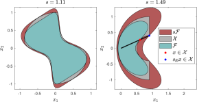
Figure 2: 4th-order approximations of star-convex set (left) and non-star-convex set (right) found by minimizing scaling term $s$. The non-star-convex set has a lower bound $s_{lb}>1$ on the achievable approximation scaling $s$.

Remark 1.

Our scaling heuristic is applicable to approximating any compact set containing the origin in its interior. However, it is best suited to approximating star-convex sets in which $0\in\textup{int}\mathcal{X}\cap\textup{ker}\,\mathcal{X}$ as visualized in Figure 2. Otherwise there exists a lower bound $s_{lb}$ such that $1<s_{lb}\leq s$ in (2).

Lemma 3.

Let $\mathcal{X}$ and $\mathcal{F}$ be compact sets in $\mathbb{R}^{n}$. Let $\mathcal{F}\subseteq\mathcal{X}\subseteq s^{\star}\mathcal{F}$ for some $s^{\star}>1$. Let $0\in\textup{int }\mathcal{F}$. Let $x,sx\in\mathcal{X}$ and $tx\not\in\mathcal{X}\,\forall\,t\in(1,s)$ for some $s>1,x\neq 0$. Then $s^{\star}\geq s$.

Proof.

See appendix.∎

We let $s_{lb}$ denote the greatest lower bound given by Lemma 3. This imposes a minimum volume ratio between the inner and outer approximation. Figure 2 (right) visualizes this result. The set is not star-convex and therefore $0\not\in\textup{ker}\mathcal{X}$. The black line segment connecting the origin to point $s_{lb}x$ is not contained in $\mathcal{X}$. This point imposes a lower bound on $s$, preventing the inner and outer approximations from coming closer together.

We introduce SOS polynomials $\lambda_{i}(x),\mu_{i}(x),i\in[m]$ and replace the set-containment conditions in (2) with SOS conditions. If $s$ is left as a decision variable, we would have bilinear terms involving the coefficients of $f(x)$ and $s$. Instead we perform a bisection over $s$, solving a feasibility problem at each iteration as given by (1). Algorithm 1 details the bisection method.

Optimization Problem: FindApprox($s,g_{i}$) —s— f(x), λ_i(x), μ_i(x)0 f(x) - (1+ϵ) - λ_i(x)(g_i(x)-1)∈Σ[x] , i ∈[m], 1-f(xs) - ∑_i=1^m μ_i(x)(1-g_i(x))∈Σ[x] , λ_i(x), μ_i(x)∈Σ[x] ,           i ∈[m].

Algorithm 1 Inner and Outer Approximation of $\mathcal{X}$

0:  $\mathcal{X}=\{x\in\mathbb{R}^{n}\,|\,g_{i}(x)\leq 1,i\in[m]\}$, $s_{tol}>0$

0:  $\mathcal{F},s\mathcal{F}\textup{ s.t. }\mathcal{F}\subseteq\mathcal{X}\subseteq s\mathcal{F}$

  $s_{ub}\leftarrow 1+s_{tol},s_{lb}\leftarrow 1$

  while FindApprox($s_{ub},g_{i})=\textup{Infeasible}$ do

     $s_{lb}\leftarrow s_{ub}$

     $s_{ub}\leftarrow 2s_{ub}$

  while $s_{ub}-s_{lb}>s_{tol}$ do

     $s_{try}\leftarrow 0.5(s_{ub}+s_{lb})$

     if FindApprox($s_{try},g_{i})=\textup{Infeasible}$ then

        $s_{lb}\leftarrow s_{try}$

     else

        $s_{ub}\leftarrow s_{try}$

  return  FindApprox($s_{ub},g_{i})$

Remark 2.

The objective is scale-invariant. Let solution $(f^{*}(x),s^{*})$ define an outer and inner approximation of $\mathcal{X}$. Scale $\mathcal{X}$ by $\alpha>0$, replacing constraints $g_{i}(x)$ with $g_{i}(\frac{x}{\alpha})$. Then the solution pair $(f^{*}(\tfrac{x}{\alpha}),s^{*})$ defines the new approximation, where the objective value remains unchanged. The objective is not translation-invariant however. For example, assume we approximate a star-convex set exactly with $(f^{\star}(x),s^{\star}=1)$. Translate $\mathcal{X}$ by $t\in\mathcal{X}\setminus\textup{ker}\mathcal{X}$, replacing $g_{i}(x)$ with $g_{i}(x-t)$. Then $0\not\in\textup{ker}\mathcal{X}$ and $s^{\star}>1$ for any approximation by Lemma 3.

Remark 3.

If $\mathcal{F}$ is convex we can relate the scaling $s$ to the Hausdorff distance between the approximations.

Lemma 4.

Let $\mathcal{F}\subset\mathbb{R}^{n}$ be a convex, compact set and $s\geq 1$. Then the following holds:

$$d_{H}(s\mathcal{F},\mathcal{F})=(s-1)\cdot\underset{x\in\mathcal{F}}{\textup{max}}\|x\|_{2}.$$ (9)

Proof.

See appendix.∎

V Sampling-Based Approximations of the Kernel

Algorithm 1 assumed the set $\mathcal{X}$ contained the origin in its kernel. If this does not hold, but there exists a point $x^{\star}\in\textup{ker}\mathcal{X}\cap\textup{int}\mathcal{X}$ we can apply Algorithm 1 to the translated set $\{x-x^{*}\,|\,x\in\mathcal{X}\}$. As our objective is not invariant with respect to translation, it is useful to approximate the kernel to establish possible choices for $x^{\star}$. In this section we provide algorithms for finding polytopic approximations of $\textup{ker}\,\mathcal{X}$.

It will be convenient to represent the boundary of $\mathcal{X}$ in terms of the inequality that is active. Define the following:

$$\partial\mathcal{X}_{i}=\{x\,|\,g_{i}(x)=1,g_{j}(x)\leq 1,j\in[m]\setminus i\}.$$ (10)

The boundary of $\mathcal{X}$ is given by the union

$$\partial\mathcal{X}=\bigcup_{i\in[m]}\partial\mathcal{X}_{i}.$$ (11)

Lemma 5.

Let $\mathcal{X}$ be a semialgebraic set as defined in (1). Let $\nabla g_{i}(x_{b})\neq 0\,\forall\,x_{b}\in\partial\mathcal{X}_{i},i\in[m]$. The kernel of $\mathcal{X}$ is given by the following semialgebraic set:

$$\textup{ker}\mathcal{X}=\{x_{k}\,|\,\nabla g_{i}(x_{b})^{T}(x_{k}-x_{b})\leq 0\,\forall\,x_{b}\in\partial\mathcal{X}_{i},i\in[m]\}.$$

Proof.

See appendix.∎

Remark.

From Lemma 5 we see that the kernel of $\mathcal{X}$ is defined by cutting-planes tangent to the active constraint $g_{i}(x_{b})=1,x_{b}\in\partial\mathcal{X}$ as shown in Figure 1.

Remark.

Lemma 5 assumes the gradient of an active constraint is non-zero. While restrictive, we note that this assumption is typically satisfied in sets of practical interest.

We provide sampling-based algorithms for finding outer and inner approximations of this set. If the outer approximation is empty, this is sufficient to conclude that the set $\mathcal{X}$ is not star-convex. Conversely, if the inner approximation is not empty this is sufficient to establish that $\mathcal{X}$ is star-convex. In the case that the outer approximation is not empty and the inner approximation is empty we cannot conclude anything about the star-convexity of the set.

V-A Outer Approximation

We assume the existence of an oracle $\text{Sample}(\partial\mathcal{X})$ which allows us to randomly sample points $x_{b}\in\partial\mathcal{X}$ and identify the set of active constraints $\mathcal{I}=\{i\,|\,i\subseteq[m],g_{i}(x_{b})=1\}$. From Lemma 5, each sample defines a cutting plane satisfied by $\textup{ker}\mathcal{X}$. We collect these constraints to form an outer approximation $\mathcal{K}_{o}\supseteq\textup{ker}\mathcal{X}$. If at any point, $\mathcal{K}_{o}=\emptyset$ (which can be determined using Farkas’ Lemma) we terminate as this implies $\textup{ker}\mathcal{X}=\emptyset$. Algorithm 2 summarizes the method.

Algorithm 2 Outer Approximation of $\textup{ker}\mathcal{X}$

0:  $\mathcal{X}=\{x\in\mathbb{R}^{n}\,|\,g_{i}(x)\leq 1,i\in[m]\}$, $n_{s}\geq 1$

0:  Outer Approximation $\mathcal{K}_{o}\supseteq\textup{ker}\mathcal{X}$

  $\mathcal{K}_{o}\leftarrow\mathbb{R}^{n}$

  for $j=1$ to $n_{s}$ do

     $x_{b},\mathcal{I}\leftarrow\text{Sample}(\partial\mathcal{X})$

     $\mathcal{K}_{o}\leftarrow\mathcal{K}_{o}\bigcap\{x\,|\,\nabla g_{i}^{T}(x_{b})(x-x_{b})\leq 0,i\in\mathcal{I}\}$

     if ($\mathcal{K}_{o}=\emptyset$) then

        return  $\mathcal{K}_{o}$

  return  $\mathcal{K}_{o}$

V-B Inner Approximation

Consider finding a point $x_{k}\in\textup{ker}\mathbf{\mathcal{X}}$ that maximizes a linear cost $c^{T}x_{k}$ where $c\in S^{n-1}$ (i.e. the support function of $\textup{ker}\mathbf{\mathcal{X}}$). From Lemma 5, the resulting convex optimization problem requires set containment constraints: —s— x_kc^Tx_k -∇g_i(x)^T(x_k - x) ≥0   ∀  x ∈∂X_i,   i ∈[m].

We replace the set containment conditions with SOS conditions using Putinar’s Positivstellensatz [14].
Optimization Problem: FindSupport$(c,g_{i})$ —s— x_k, λ_j^(i)(x)c^Tx_k -​∇g_i(x)^T(x_k ​ - x) ​ - ​ ∑j=1m λj(i)(x)(1 ​- ​ gj(x))∈Σ[x] ,  i ∈[m] λ_j^(i)(x)∈Σ[x] ,       i ∈[m], j ∈[m] ∖i.

For a given direction $c\in S^{n-1}$ this program lower bounds the support function of $\textup{ker}\mathcal{X}$. The lower bound monotonically increases with $\textup{deg}(\lambda_{j}^{(i)})$. If the problem is feasible, the maximizing argument $x_{k}$ belongs to $\textup{ker}\mathcal{X}$ and therefore $\mathcal{X}$ is star-convex. If infeasible we cannot make any conclusions about the star-convexity of $\mathcal{X}$. By solving for random directions $c_{i}\in S^{n-1},i\in[n_{s}]$ the convex hull of points $x_{k}$ provides an inner approximation of the kernel as given by Algorithm 3.

Algorithm 3 Inner Approximation of $\textup{ker}\mathcal{X}$

0:  $\mathcal{X}\!=\!\{x\!\in\!\mathbb{R}^{n}|g_{i}(x)\!\leq\!1,i\!\in\![m]\}$,​ $\{c_{i}\}\!\subset\!S^{n-1},i\!\in\![n_{s}]$

0:  Inner Approximation $\mathcal{K}_{i}\subseteq\textup{ker}\mathcal{X}$

  $\mathcal{K}_{i}\leftarrow\emptyset$

  for $j=1$ to $n_{s}$ do

     $x_{k}\leftarrow\textup{FindSupport}(c_{j},g_{i})$

     if $\textup{FindSupport}(c_{j},g_{i})$ = Infeasible then

        return  $\mathcal{K}_{i}=\emptyset$

     $\mathcal{K}_{i}\leftarrow\textup{conv}(\mathcal{K}_{i},x_{k})$

  return  $\mathcal{K}_{i}$

V-C Kernel of Unions and Intersections

Given sets $\mathcal{A},\mathcal{B}\subseteq\mathbb{R}^{n}$ and their kernels, we can find inner approximations of the kernel of their intersection and union using the following lemma.

Lemma 6.

Let $\mathcal{A},\mathcal{B}\subseteq\mathbb{R}^{n}$. Then the following holds:

$$\textup{ker}(\mathcal{A}\cap\mathcal{B}) \supseteq\textup{ker}\mathcal{A}\cap\textup{ker}\mathcal{B}$$ (12)

$$\textup{ker}(\mathcal{A}\cup\mathcal{B}) \supseteq\textup{ker}\mathcal{A}\cap\textup{ker}\mathcal{B}.$$ (13)

Proof.

See appendix.∎

Thus if $\mathcal{A},\mathcal{B}$ are star-convex and have kernels that intersect, their union and intersection is also star-convex. This is useful for establishing star-convexity without resorting to numerical algorithms.

VI Examples

We evaluate Algorithm 1 on various examples and compare the results to the existing heuristics reviewed in Section III. We focus our comparison on outer approximations as more heuristics apply to this case. We use percent error as our metric, calculated as $100\times\frac{\textup{vol}\mathcal{F}_{o}-\textup{vol}\mathcal{X}}{\textup{vol}\mathcal{X}}$ where $\mathcal{F}_{o}$ is the outer approximation of $\mathcal{X}$. We first consider approximating two examples from the literature with polynomials of increasing degree. In all instances, our algorithm yielded the tightest outer approximation as shown in Figure 3. Next we consider 100 randomly generated convex polytopes in $\mathbb{R}^{2}$. In the majority of cases, our heuristic yielded the tightest outer approximation as shown in Table I. Lastly, we approximate a set that is not star-convex. Our heuristic degrades with increasing lower bound $s_{lb}$ as suggested by Lemma 3.

VI-A Polynomial matrix inequality [3]

$$\mathcal{X}=\{x\in\mathbb{R}^{2}\,|\,\begin{bmatrix}1-16x_{1}x_{2}&x_{1}\\ x_{1}&1-x_{1}^{2}-x_{2}^{2}\end{bmatrix}\succeq 0\}.$$

Using Algorithms 2 and 3 we find the kernel ($\mathcal{K}_{o}=\mathcal{K}_{i}=\textup{conv}\{\pm(-0.1752,0.3335),\pm(0.1268,0.2213)\}$) as shown in Figure 1. Figure 2 (left) shows the 4th-order approximation obtained with Algorithm 1. Figure 3 shows the percent error as we increase the degree. Although each objective value (not shown) decreases monotonically with increasing degree, the percent error occasionally increases. This demonstrates the heuristic nature of the objectives for minimizing volume.

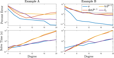
Figure 3: Approximation percent error and solve times for examples A and B. Solve times shown for objective $s$ are for one $\textup{FindApprox}(s,g_{i})$ iteration.

VI-B Discrete-time stabilizability region [3],[1]

$$\mathcal{X}=\{x\in\mathbb{R}^{2}\,|\,1+2x_{2}\geq 0,2-4x_{1}-3x_{2} \geq 0,$$

$$10-28x_{1}-5x_{2}-24x_{1}x_{2}-18x_{2}^{2} \geq 0,$$

$$1-x_{2}-8x_{1}^{2}-2x_{1}x_{2}-x_{2}^{2}-8x_{1}^{2}x_{2}-6x_{1}x_{2}^{2} \geq 0\}.$$

The set contains the origin in its kernel. Figure 3 shows the percent error for increasing degree. Figure 4 shows the 6th-order approximations obtained with each objective. For the $l_{1}$ approximation we also show the bounding box from [1].

VI-C Convex Polytopes

We generate 100 random convex polytopes in $\mathbb{R}^{2}$ with their Chebyshev center at the origin. We find outer approximations using the different objectives. Table I lists the number of times each objective obtained the smallest percent error relative to the other objectives for a given polytope.

TABLE I: Instances In Which Objective Obtained Smallest Error

Deg.	# Trials	$s$	$-\textup{det}P$	$\textup{tr}P^{-1}$	$l_{1}$
4	100	73	13	0	14
6	100	98	0	0	2

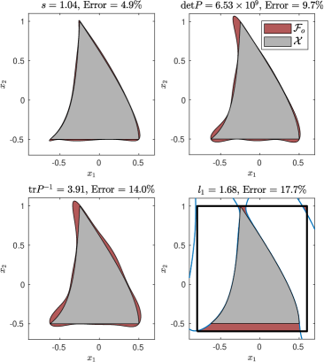
Figure 4: 6th-order outer approximations of example B

VI-D Non-Star-Convex Set

$$\mathcal{X}=\{x\in\mathbb{R}^{2}\,|\,r^{2}\leq(x_{1}-c)^{2}+x_{2}^{2}\leq 1,x_{1}\leq c\}.$$

Let $0<r<c<1$ so the origin is in the interior of the set. Figure 2 shows the set for the case in which $c=0.9$ and $r=0.4$. Points $(c,\pm r)\in\partial\mathcal{X}$ yield cutting planes $x_{2}\geq r$ and $x_{2}\leq-r$ such that $\textup{ker}\mathcal{X}=\emptyset$. Table II gives the outer approximation error for $c=0.9$ and varying $r$. For the scaling objective, we also report the objective value $s^{\star}$ and its lower bound $s_{lb}$. As $s_{lb}$ increases the percent error increases, confirming our heuristic is best suited to star-convex sets.

TABLE II: Percent Error of Outer Approximations of Example E

r	Degree	$s(s^{\star}/s_{lb})$	$-\textup{det}P$	$\textup{tr}P^{-1}$
0.1	4	12.0 (1.096 / 1.025)	13.0	11.8
0.2	4	13.6 (1.104 / 1.104)	16.1	14.0
0.3	4	35.1 (1.250 / 1.250)	18.5	17.8
0.4	4	81.7 (1.492 / 1.492)	17.3	22.9

VI-E Solver Performance

Figure 3 shows the solve times for the various objectives on a logarithmic scale. Applied to a matrix $P\in\mathbb{R}^{m\times m}$, the $-\textup{det}P$ and $\textup{tr}P^{-1}$ objectives introduce a PSD matrix $H\in\mathbb{R}^{2m\times 2m}$ due to reformulations involving the exponential cone [15] and Schur complement [4] respectively. In contrast, the scaling $(s)$ and $l_{1}$ objectives work directly with $P$, yielding smaller semidefinite programs. The $l_{1}$ objective has the best computational performance. Due to the use of bisection, the total solve time for the scaling objective is an integer multiple of the time shown in Figure 3. Accounting for this, the scaling objective still remains competitive with the $-\textup{det}P$ and $\textup{tr}P^{-1}$ objectives.

VI-F Implementation Details

YALMIP [16] and MOSEK [15] were used to solve the SOS programs. Volumes of non-star-convex sets were approximated by evaluating the indicator function over a discrete grid. Volumes of star-convex sets were approximated using numerical integration in polar coordinates.

VII CONCLUSIONS

An algorithm for finding approximations of semialgebraic sets using sum-of-squares optimization was proposed. The algorithm relies on a novel objective which minimizes the scaling necessary to transform an inner approximation into an outer approximation of the set. Numerical examples demonstrated this objective often finds tighter approximations compared to existing heuristics when applied to star-convex sets. Applied to non-star-convex sets, our proposed heuristic performs poorly. A promising direction to address this is through star-convex decompositions [17]. We leave this exploring this option for future work.

References

- [1] F. Dabbene, D. Henrion, and C. M. Lagoa, “Simple approximations of semialgebraic sets and their applications to control,” Automatica, vol. 78, pp. 110–118, 2017.
- [2] A. Magnani, S. Lall, and S. Boyd, “Tractable fitting with convex polynomials via sum-of-squares,” in Proceedings of the 44th IEEE Conference on Decision and Control, pp. 1672–1677, 2005.
- [3] D. Henrion and J.-B. Lasserre, “Inner approximations for polynomial matrix inequalities and robust stability regions,” IEEE Transactions on Automatic Control, vol. 57, no. 6, pp. 1456–1467, 2012.
- [4] A. A. Ahmadi, G. Hall, A. Makadia, and V. Sindhwani, “Geometry of 3d environments and sum of squares polynomials,” in Robotics: Science and Systems, 2017.
- [5] V. Cerone, D. Piga, and D. Regruto, “Polytopic outer approximations of semialgebraic sets,” in 2012 IEEE 51st IEEE Conference on Decision and Control (CDC), pp. 7793–7798, 2012.
- [6] J. Guthrie and E. Mallada, “Outer approximations of minkowski operations on complex sets via sum-of-squares optimization,” in 2021 American Control Conference (ACC), pp. 2367–2373, 2021.
- [7] J. Guthrie, M. Kobilarov, and E. Mallada, “Closed-form minkowski sum approximations for efficient optimization-based collision avoidance,” in 2022 American Control Conference (ACC), 2022.
- [8] M. Jones and M. M. Peet, “Using sos for optimal semialgebraic representation of sets: Finding minimal representations of limit cycles, chaotic attractors and unions,” in 2019 American Control Conference (ACC), pp. 2084–2091, 2019.
- [9] J.-B. Lasserre, “A generalization of löwner-john’s ellipsoid theorem,” Mathematical Programming, vol. 152, 08 2014.
- [10] P. Parrilo, Structured semidefinite programs and semialgebraic geometry methods in robustness and optimization. PhD thesis, California Institute of Technology, 2000.
- [11] H. Brunn, “Über kerneigebiete,” Math. Ann., vol. 93, p. 436–440, 1913.
- [12] D. Henrion, J.-B. Lasserre, and C. Savorgnan, “Approximate volume and integration for basic semialgebraic sets,” SIAM Review, vol. 51, pp. 722–743, 11 2009.
- [13] M. Korda and D. Henrion, “Convergence rates of moment-sum-of-squares hierarchies for volume approximation of semialgebraic sets,” Optimization Letters, vol. 12, pp. 435–442, 2018.
- [14] M. Putinar, “Positive polynomials on compact semi-algebraic sets,” Indiana University Mathematics Journal, vol. 42, no. 3, pp. 969–984, 1993.
- [15] M. ApS, The MOSEK optimization toolbox for MATLAB manual. Version 8.1., 2017.
- [16] J. Lofberg, “Yalmip : a toolbox for modeling and optimization in matlab,” in 2004 IEEE International Conference on Robotics and Automation (IEEE Cat. No.04CH37508), pp. 284–289, Sep. 2004.
- [17] N. Delanoue, L. Jaulin, and B. Cottenceau, “Using interval arithmetic to prove that a set is path-connected,” Theoretical Computer Science, vol. 351, pp. 119–128, 2006.