On the characteristic polynomial of an effective Hamiltonian

Abstract

The characteristic polynomial of the effective Hamiltonian for a general model has been discussed. It is found that, compared with the associated energy eigenvalues, this characteristic polynomial generally has better analytical properties and larger convergence radius when being expanded in powers of the interaction parameter, and hence is more suitable for a perturbation calculation. A form of effective Hamiltonian which has the same singularities (branch points) as such characteristic polynomial has also been constructed.

1 Introduction

Many quantum interaction models, such as the Hubbard model and nuclear-shell model, involve states with different energy scales. If one is only interested in some special states, say, the lower-energy-scale states, the full Hilbert space of the model can be partitioned into two disjoint subspaces: the so-called $P$- and $Q$-spaces, which are spanned by the states we are interested and uninterested in respectively. For a full Hamiltonian $H(\lambda)$ with an interaction parameter $\lambda$, an effective elimination of the states we are uninterested in, via rigorous perturbation treatment or canonical transformation, etc., can yield a dimension-reduced equivalent Hamiltonian which only acts on the $P$-space or the remaining states, the so-called effective Hamiltonian $H_{\mathrm{eff}}(\lambda)$ (For recent and historical references of this, see Refs. [1, 2, 3, 4, 5, 6, 7]).

The obtained $H_{\mathrm{eff}}(\lambda)$ generally is complicated and always in an infinite series form of the interaction parameter $\lambda$, from which the further solving process for interesting physical quantities such as the energy eigenvalues is still nontrivial. On the other hand, the convergence problem of such series-form of $H_{\mathrm{eff}}(\lambda)$ itself is difficult to discuss [1, 2]. Especially, the effective Hamiltonian can be derived by several ways, e.g., by block-diagonalization of $H(\lambda)$ via similarity transformation, Rayleigh-Schrödinger or Brillouin-Wigner Perturbation. Different derivation procedures usually lead to different series-forms of $H_{\mathrm{eff}}(\lambda)$, which can be energy-dependent or energy-independent, Hermitian or Non-Hermitian [4, 5]. Mathematically, even for the same problem, there are infinitely many $H_{\mathrm{eff}}(\lambda)$ which are similar matrices to each other [8, 9]. This makes the theory of effective Hamiltonian lack unity in some sense.

It is interesting whether the effective Hamiltonian can be discussed in a more unified and efficient way. Here we want to study $H_{\mathrm{eff}}(\lambda)$ from another point of view, i.e., via discussing its characteristic polynomial $\det[E-H_{\mathrm{eff}}(\lambda)]$. One consideration of our discussion is that though the effective Hamiltonian can be in different Matrix forms similar to each other, the characteristic polynomial is unique. This may enable us to study some essential properties of the effective Hamiltonian itself, rather than those only associated with its some particular form. Additionally, we will find that the characteristic polynomial itself has some very important characteristics, such as that it always has less singularities in the complex plane of $\lambda$ than the $P$-space energy eigenvalues, which would allow us to perform a more effective perturbation treatment even when the detailed form of $H_{\mathrm{eff}}(\lambda)$ is unknown.

2 Formulation

We consider a system of dimension $\tilde{N}=N+M$, of which the model space can be decoupled into two subspaces: a $P$-space spanned by $N$ states of interesting and a $Q$-space spanned by the other $M$ states. The Hamiltonian can be written as

$$H(\lambda)=H_{0}+\lambda H_{I},$$ (1)

where $H_{0}$ and $H_{I}$ both are Hermitian:

$$H_{0}=\sum_{n=1}^{N}\epsilon_{n}^{{}_{P}}|\psi^{{}_{P}}_{n}\rangle\langle\psi^{{}_{P}}_{n}|+\sum_{n=1}^{M}\epsilon_{n}^{{}_{Q}}|\psi^{{}_{Q}}_{n}\rangle\langle\psi^{{}_{Q}}_{n}|,$$

$$H_{I}=\sum_{n,m}h^{\!{}_{P}}_{mn}|\psi^{{}_{P}}_{n}\rangle\langle\psi^{{}_{P}}_{m}|+\sum_{n,m}h^{\!{}_{Q}}_{mn}|\psi^{{}_{Q}}_{n}\rangle\langle\psi^{{}_{Q}}_{m}|+\sum_{n,m}\left[h^{\!{}_{P\!Q}}_{mn}|\psi^{{}_{P}}_{n}\rangle\langle\psi^{{}_{Q}}_{m}|+\text{h.c}\right],$$

Without losing generality, we assume that the unperturbed energies of $P$- and $Q$-space states all are non-degenerate, i.e., $\epsilon_{1}^{{}_{P}}\neq\epsilon_{2}^{{}_{P}}$, $\epsilon_{1}^{{}_{P}}\neq\epsilon_{1}^{{}_{Q}}$, etc. For small $\lambda$, the eigenvalues of $P$-space states, $E_{1}^{{}_{P}}(\lambda),E_{2}^{{}_{P}}(\lambda),\cdots,E_{N}^{{}_{P}}(\lambda)$ can be expanded as

$$E_{1}^{{}_{P}}=\epsilon_{1}^{{}_{P}}+\lambda h^{\!{}_{P}}_{11}+\lambda^{2}\left(\sum_{n\neq 1}\frac{|h^{\!{}_{P}}_{1n}|^{2}}{\epsilon_{1}^{{}_{P}}-\epsilon_{n}^{{}_{P}}}+\sum_{n}\frac{|h^{\!{}_{P\!Q}}_{1n}|^{2}}{\epsilon_{1}^{{}_{P}}-\epsilon_{n}^{{}_{Q}}}\right)+\cdots$$ (2.1)

$$E_{2}^{{}_{P}}=\epsilon_{2}^{{}_{P}}+\lambda h^{\!{}_{P}}_{22}+\lambda^{2}\left(\sum_{n\neq 2}\frac{|h^{\!{}_{P}}_{2n}|^{2}}{\epsilon_{2}^{{}_{P}}-\epsilon_{n}^{{}_{P}}}+\sum_{n}\frac{|h^{\!{}_{P\!Q}}_{2n}|^{2}}{\epsilon_{2}^{{}_{P}}-\epsilon_{n}^{{}_{Q}}}\right)+\cdots$$ (2.2)

$$\quad\cdots\cdots$$

$$E_{N}^{{}_{P}}=\epsilon_{N}^{{}_{P}}+\lambda h^{\!{}_{P}}_{N\!N}+\lambda^{2}\left(\sum_{n\neq N}\frac{|h^{\!{}_{P}}_{Nn}|^{2}}{\epsilon_{N}^{{}_{P}}-\epsilon_{n}^{{}_{P}}}+\sum_{n}\frac{|h^{\!{}_{P\!Q}}_{Nn}|^{2}}{\epsilon_{N}^{{}_{P}}-\epsilon_{n}^{{}_{Q}}}\right)+\cdots.$$ (2.N)

Similar expressions can also be written out for the eigenvalues of $Q$-space states $E_{1}^{{}_{Q}}(\lambda),E_{2}^{{}_{Q}}(\lambda),\cdots,E_{M}^{{}_{Q}}(\lambda)$. These expansion series always break down when $\lambda$ is adequately large. This is due to the fact that the $E_{n}^{{}_{P}}(\lambda)$ and $E_{m}^{{}_{Q}}(\lambda)$, as functions of $\lambda$, generally have singularities in the complex plane of $\lambda$. The convergence radius of the expansion series is determined by the module of the singularity closest to the origin, for each $E_{n}^{{}_{P}}(\lambda)$ or $E_{m}^{{}_{Q}}(\lambda)$. Mathematically, since $E_{n}^{{}_{P}}$ and $E_{m}^{{}_{Q}}$ are solutions of the algebraic equation $\det[E-H(\lambda)]=0$, the only singularities are branch points [10, 11, 12]. Here,

$$\det[E-H(\lambda)]=\prod_{n=1}^{N}[E-E_{n}^{{}_{P}}(\lambda)]\prod_{m=1}^{M}[E-E_{m}^{{}_{Q}}(\lambda)]\\ =E^{\tilde{N}}+p_{1}(\lambda)E^{\tilde{N}-1}+\cdots+p_{\tilde{N}-1}(\lambda)E+p_{\tilde{N}}(\lambda),$$ (3)

with the coefficients $p_{n}(\lambda)$ being polynomials of $\lambda$.

As is well-known, these branch points are characterized by “level-crossing”, where two (or more) eigenvalues, accompanying their eigenfunctions, coincide. Level-crossings can occur between two $P$-space states ($PP$-crossing), two $Q$-space states ($QQ$-crossing), or one $P$-space state and one $Q$-space state ($PQ$-crossing). Hence, if some $\lambda$ in the complex plane is a branch point of eigenvalue $E_{n}^{{}_{P(Q)}}(\lambda)$, it must also be a branch point of at least one other eigenvalue. For each $E_{n}^{{}_{P}}(\lambda)$ or $E_{m}^{{}_{Q}}(\lambda)$, the branch-point set can be denoted by $\{\lambda^{{}_{P}}_{n,l_{n}},\lambda^{{}_{PQ}}_{n,l^{\prime}_{n}}\}$ or $\{\lambda^{{}_{Q}}_{m,l_{m}},\lambda^{{}_{QP}}_{m,l^{\prime}_{m}}\}$ respectively, with the $\lambda^{{}_{P(Q)}}_{i,l_{i}}$ or $\lambda^{{}_{PQ(QP)}}_{i,l^{\prime}_{i}}$ representing the branch points due to the level-crossing of $E_{i}^{{}_{P(Q)}}(\lambda)$ with the other $E_{j}^{{}_{P(Q)}}(\lambda)$ or $E_{j}^{{}_{Q(P)}}(\lambda)$ respectively, which are numbered by $l_{i}(l^{\prime}_{i})=1,2,\cdots$. For example, if $E_{1}^{{}_{P}}(\lambda)$ only has five branch points, three due to $PP$-crossing and two due to $PQ$-crossing, we have $\{\lambda^{{}_{P}}_{1,l_{1}},\lambda^{{}_{PQ}}_{1,l^{\prime}_{1}}\}=\{\lambda^{{}_{P}}_{1,1},\lambda^{{}_{P}}_{1,2},\lambda^{{}_{P}}_{1,3},\lambda^{{}_{PQ}}_{1,1},\lambda^{{}_{PQ}}_{1,2}\}$.

Then, the convergence radius of the $E_{n}^{{}_{P}}$-series is determined by $r_{n}^{{}_{P}}=\min_{l_{n},l^{\prime}_{n}}\{|\lambda^{{}_{P}}_{n,l_{n}}|,|\lambda^{{}_{PQ}}_{n,l^{\prime}_{n}}|\}$. We can further introduce a common convergence radius for these $E_{n}^{{}_{P}}$-series,

$$\bar{r}^{{}_{P}}=\min_{n}\{r_{n}^{{}_{P}}\}=\min_{l_{1},l^{\prime}_{1},\cdots,l_{N},l^{\prime}_{N}}\{\lambda^{{}_{P}}_{1,l_{1}},\lambda^{{}_{PQ}}_{1,l^{\prime}_{1}},\cdots,\lambda^{{}_{P}}_{N,l_{N}},\lambda^{{}_{PQ}}_{N,l^{\prime}_{N}}\}.$$ (4)

Obviously, $\bar{r}^{{}_{P}}$ specifies the maximum $|\lambda|$ for which all the $E_{n}^{{}_{P}}$-series converge.

Mathematically, if some branch points, say these due to $PP$-crossing, can be removed, enlarged convergence radii may be obtained for the perturbation calculation of $E_{n}^{{}_{P}}$. Our strategy is to use the characteristic polynomial of $H_{\mathrm{eff}}(\lambda)$,

$$\det[E-H_{\mathrm{eff}}(\lambda)]=\prod_{n=1}^{N}[E-E_{n}^{{}_{P}}(\lambda)]=E^{N}-P_{1}(\lambda)E^{N-1}\\ +\cdots+(-1)^{N-1}P_{N-1}(\lambda)E+(-1)^{N}P_{N}(\lambda),$$ (5)

where the coefficients are symmetric polynomials of $P$-space eigenvalues,

$$P_{1}(\lambda)=E_{1}^{{}_{P}}(\lambda)+E_{2}^{{}_{P}}(\lambda)+\cdots+E_{N}^{{}_{P}}(\lambda),$$ (6.1)

$$P_{2}(\lambda)=\sum_{1\leq j_{1}<j_{2}\leq N}E_{j_{1}}^{{}_{P}}(\lambda)E_{j_{2}}^{{}_{P}}(\lambda),$$ (6.2)

$$\quad\cdots\cdots$$

$$P\!_{N}(\lambda)=E_{1}^{{}_{P}}(\lambda)E_{2}^{{}_{P}}(\lambda)\cdots E_{N}^{{}_{P}}(\lambda).$$ (6.N)

Unlike what in Eq. (3), since the detailed form of $H_{\mathrm{eff}}(\lambda)$ has not been specified, the coefficients $P_{n}(\lambda)$ in Eq. (5) is unknown; however, we can calculate them using Eqs. (6.1)–(6.N), i.e., by their relationship with $E_{n}^{{}_{P}}(\lambda)$, since $E_{n}^{{}_{P}}(\lambda)$ can be calculated via the perturbation expansion as shown above. We first discuss the availability of such calculation for $P_{n}(\lambda)$.

Noting that both $\det[E-H_{\mathrm{eff}}(\lambda)]$ and $P_{n}(\lambda)$ are unchanged under the exchange of any two $P$-space eigenvalues, say, $E_{i}^{{}_{P}}(\lambda)$ and $E_{j}^{{}_{P}}(\lambda)$, one can expect that the $PP$-crossing of $P$-space eigenvalues would not cause branch points for them. This can be demonstrated in more detail as follows. For any finite $\lambda$-region we want to discuss, Eq. (3) can be further written as

$$\prod_{n=1}^{N}[E-E_{n}^{{}_{P}}(\lambda)]=\frac{\det[E-H(\lambda)]}{\prod_{m=1}^{M}[E-E_{m}^{{}_{Q}}(\lambda)]},$$ (7)

where $E$ is viewed as a constant and takes its value large enough, say, outside the Gerschgorin disks of the $E_{m}^{{}_{Q}}(\lambda)$, to ensure a nonzero denominator of the right-hand side of the equation. One should note that the left-hand side of this equation just has the form of $\det[E-H_{\mathrm{eff}}(\lambda)]$.

Although $E_{n}^{{}_{P}}(\lambda)$ and $E_{m}^{{}_{Q}}(\lambda)$ each may have several branch points in the complex plane of $\lambda$, the true branch points $\lambda_{c}$ of the right or left side of Eq. (7) can only be the those which are the common branch points of the both sides. Noting that here $\det[E-H(\lambda)]$, as shown in Eq. (3), has no branch point in the complex plane of $\lambda$, the only common branch points certainly are these due to the $PQ$-crossing of $E_{n}^{{}_{P}}(\lambda)$ and $E_{m}^{{}_{Q}}(\lambda)$, which constitute a set $S_{PQ}\equiv\{\lambda^{{}_{PQ}}_{1,l_{1}},\lambda^{{}_{PQ}}_{2,l_{2}},\cdots,\lambda^{{}_{PQ}}_{N,l_{N}}\}$, with the serial numbers $l_{n}=1,2,\cdots$ as above. Namely, unlike in the case of $E_{n}^{{}_{P}}(\lambda)$ and $E_{m}^{{}_{Q}}(\lambda)$, the $PP$- or $QQ$-crossing does not cause any branch points for $\prod_{n=1}^{N}[E-E_{n}^{{}_{P}}(\lambda)]$ (i.e., $\det[E-H_{\mathrm{eff}}(\lambda)]$) and $\prod_{m=1}^{M}[E-E_{m}^{{}_{Q}}(\lambda)]$.

Hence, the characteristic polynomial $\det[E-H_{\mathrm{eff}}(\lambda)]$, as a function of $\lambda$, is “more analytical” than $E_{n}^{{}_{P}}(\lambda)$, and more suitable for a perturbation calculation.

To illustrate this more simply, we can first discuss the case of $N=2$:

$$\det[E-H_{\mathrm{eff}}(\lambda)]=E^{2}-P_{1}(\lambda)E+P_{2}(\lambda),$$ (8)

for which, the set of the only branch points becomes $S_{PQ}=\{\lambda^{{}_{PQ}}_{1,l_{1}},\lambda^{{}_{PQ}}_{2,l_{2}}\}$.

The branch-point set of $P_{1}(\lambda)$ and $P_{2}(\lambda)$ must be the same as $S_{PQ}$. Namely, unlike $E^{{}_{P}}_{1}(\lambda)$ and $E^{{}_{P}}_{2}(\lambda)$, $P_{1}(\lambda)$ and $P_{2}(\lambda)$ also do not have branch points due to the $PP$-crossing.

Therefore, unlike $E^{{}_{P}}_{1}(\lambda)$- or $E^{{}_{P}}_{2}(\lambda)$-series, the expansions

$$P_{1}(\lambda) =E_{1}^{{}_{P}}(\lambda)+E_{2}^{{}_{P}}(\lambda)$$

$$=\epsilon_{1}^{{}_{P}}+\epsilon_{2}^{{}_{P}}+\lambda(h^{\!{}_{P}}_{11}+h^{\!{}_{P}}_{22})+\lambda^{2}\sum_{i=1,2}\sum_{n}\frac{|h^{\!{}_{P\!Q}}_{in}|^{2}}{\epsilon_{i}^{{}_{P}}-\epsilon_{n}^{{}_{Q}}}+\cdots,$$

$$P_{2}(\lambda) =E_{1}^{{}_{P}}(\lambda)E_{2}^{{}_{P}}(\lambda)=\epsilon_{1}^{{}_{P}}\epsilon_{2}^{{}_{P}}+\lambda\left(\epsilon^{{}_{P}}_{1}h^{{}_{P}}_{22}+\epsilon^{{}_{P}}_{2}h^{{}_{P}}_{11}\right)$$

$$\quad+\lambda^{2}\Big{[}h^{{}_{P}}_{11}h^{{}_{P}}_{22}-|h^{\!{}_{P}}_{12}|^{2}+\sum_{n}\Big{(}\frac{\epsilon^{{}_{P}}_{1}|h^{\!{}_{P\!Q}}_{2n}|^{2}}{\epsilon_{2}^{{}_{P}}-\epsilon_{n}^{{}_{Q}}}+\frac{\epsilon^{{}_{P}}_{2}|h^{\!{}_{P\!Q}}_{1n}|^{2}}{\epsilon_{1}^{{}_{P}}-\epsilon_{n}^{{}_{Q}}}\Big{)}\Big{]}+\cdots,$$

only become divergent for $|\lambda|\geq r^{{}_{P}}$, where $r^{{}_{P}}=\min_{l_{1},l_{2}}\{|\lambda^{{}_{PQ}}_{1,l_{1}}|,|\lambda^{{}_{PQ}}_{2,l_{2}}|\}$. The characteristic polynomial in Eq. (8) is further obtained and then the eigenvalues can be solved from $\det[E-H_{\mathrm{eff}}(\lambda)]=0$ as

$$E_{1,2}^{{}_{P}}(\lambda)=\frac{P_{1}(\lambda)\pm\sqrt{P_{1}(\lambda)^{2}-4P_{2}(\lambda)}}{2}.$$ (9)

Such procedure can be directly extended to a general case of $N$. Similar to the case of $N=2$, we can use the $\lambda$-expansion of $E^{{}_{P}}_{n}(\lambda)$ in Eqs. (2.1)–(2.N) to calculate $P_{n}(\lambda)$ via Eqs. (6.1)– (6.N). Also, since the branch-point set of these $P_{n}(\lambda)$ is the same as that of $\det[E-H_{\mathrm{eff}}(\lambda)]$, the convergence radius of the obtained expansions can be generally determined as

$$r^{{}_{P}}=\min_{l_{1},l_{2},\cdots,l_{N}}\{|\lambda^{{}_{PQ}}_{1,l_{1}}|,|\lambda^{{}_{PQ}}_{2,l_{2}}|,\cdots,|\lambda^{{}_{PQ}}_{N,l_{N}}|\}.$$ (10)

Once the expansion of $P_{n}(\lambda)$ has been obtained, the detailed form of $\det[E-H_{\mathrm{eff}}(\lambda)]$ can be calculated with Eq. (5). Then the $P$-space eigenvalues $E^{{}_{P}}_{n}(\lambda)$ can be solved just from

$$E^{N}-P_{1}(\lambda)E^{N-1}+\cdots+(-1)^{N-1}P_{N-1}(\lambda)E+(-1)^{N}P_{N}(\lambda)=0.$$ (11)

Obviously, for $N<5$, Eq. (11) can be solved analytically; while for $N\geq 5$, numerical methods can be employed.

Although such procedure is still a perturbative one, we can calculate $E_{n}^{{}_{P}}(\lambda)$ for $|\lambda|<r^{{}_{P}}$ in principle. Comparing Eqs. (4) and (10), we have $r^{{}_{P}}\geq\bar{r}^{{}_{P}}$. Actually, for cases that an effective Hamiltonian can be well-defined [1], the $P$- and $Q$-space eigenvalues are always “well-separated”: the $PQ$-crossing of eigenvalues only occurs when $|\lambda|$ becomes relatively large, compared with the $PP$-crossing, i.e., $r^{{}_{P}}>\bar{r}^{{}_{P}}$ or even $r^{{}_{P}}\gg\bar{r}^{{}_{P}}$; then, one can expect that with our procedure, $E_{n}^{{}_{P}}(\lambda)$ can be calculated for a larger $\lambda$-region, even far beyond the applicable scope of a direct perturbation calculation.

Additionally, $\det[E-H_{\mathrm{eff}}(\lambda)]$ also can be calculated directly with $H_{\mathrm{eff}}(\lambda)$. Certainly, this requires the the specific form of $H_{\mathrm{eff}}(\lambda)$. However, due to the uniqueness of characteristic polynomial, any expanded form of $H_{\mathrm{eff}}(\lambda)$, regardless of the convergence radius, can be used to calculate the coefficients $P_{n}(\lambda)$ and hence $\det[E-H_{\mathrm{eff}}(\lambda)]$ uniquely in powers of $\lambda$.

3 Simple example

As a simple example, we consider a case of $N=2$ and $M=1$. Due to the small dimension, it is convenient to write $H(\lambda)$ in a matrix form, which we specify as

$$H(\lambda)=\begin{bmatrix}\epsilon_{1}^{{}_{Q}}&0&0\\ 0&\epsilon_{2}^{{}_{P}}&0\\ 0&0&\epsilon_{1}^{{}_{P}}\end{bmatrix}+\lambda\begin{bmatrix}0&h^{\!{}_{Q\!P}}_{12}&0\\ h^{\!{}_{P\!Q}}_{21}&0&h^{\!{}_{P}}_{21}\\ 0&h^{\!{}_{P}}_{12}&0\end{bmatrix},$$ (12)

where we can take $\epsilon_{1}^{{}_{Q}}=2$, $\epsilon_{1}^{{}_{Q}}=1$, $\epsilon_{2}^{{}_{Q}}=1.1$ and $h^{\!{}_{P\!Q}}_{12}=h^{\!{}_{P\!Q}}_{21}=h^{\!{}_{P}}_{21}=h^{\!{}_{P}}_{12}=1$ (in arbitrary energy unit).

One purpose for us to value these quantities in this way is that in a perturbation expansion, the case of nearly-degenerate $\epsilon_{2}^{{}_{P}}$ and $\epsilon_{1}^{{}_{P}}$ is very important, since terms such as those containing “$\frac{1}{\epsilon_{2}^{{}_{P}}-\epsilon_{1}^{{}_{P}}}$” would become very large and cause divergence. Such kind of divergence problem due to the quasi-degenerate unperturbed energies is well-known, especially for the multireference perturbation theory (MRPT) in studying multiconfigurational quantum-chemical systems, and is often called the “intruder state problem” (ISP) [13, 14, 15, 16, 17]. As for our study of $H_{\mathrm{eff}}(\lambda)$, unperturbed energies $\epsilon_{n}^{{}_{P}}$ are always apart from $\epsilon_{m}^{{}_{Q}}$ far enough, and hence the ISP can occur mainly due to the quasi-degenerate $\epsilon_{n}^{{}_{P}}$, or terms containing factors such as “$\frac{1}{\epsilon_{2}^{{}_{P}}-\epsilon_{1}^{{}_{P}}}$”, which we can call the ISP terms.

This simple model can be analytically solved, and actually, a similar model has been extensively discussed in previous studies [18, 19]. To the order of $10^{-6}$, the branch points due to the $PP$-crossing of $E_{1}^{{}_{P}}(\lambda)$ and $E_{2}^{{}_{P}}(\lambda)$ are $\lambda=\pm 0.051392i$, and that due to the $PQ$-crossing of $E_{1}^{{}_{P}}(\lambda)$ and $E_{2}^{{}_{P}}(\lambda)$ with $E_{1}^{{}_{Q}}(\lambda)$ are $\lambda=-0.238116\pm 0.502871i$ and $0.238116\pm 0.502871i$ respectively. Then, the convergence radius of the $E_{1}^{{}_{P}}(\lambda)$- and $E_{2}^{{}_{P}}(\lambda)$-series is $r_{1}^{{}_{P}}=r_{2}^{{}_{P}}\approx 0.051392$, while that for the valid calculation using the characteristic polynomial is $r^{{}_{P}}\approx 0.556397$.

We have calculated $E_{1}^{{}_{P}}(\lambda)$ and $E_{2}^{{}_{P}}(\lambda)$ via our characteristic polynomial respectively for cases in which only terms through 2nd, 4th or 6th order are retained in the $\lambda$-expansion of coefficients $P_{1}(\lambda)$ and $P_{2}(\lambda)$. The results are shown in Fig. 1, and with increasing order, the obvious deviation from the exact value of $E_{1}^{{}_{P}}(\lambda)$ and $E_{2}^{{}_{P}}(\lambda)$ does tend to occur at $\lambda=r^{{}_{P}}$. As a comparison, we have also shown the result of $E_{1}^{{}_{P}}(\lambda)$ and $E_{2}^{{}_{P}}(\lambda)$ by the usual perturbation theory, i.e., via retaining terms in Eqs. (2.1) and (2.2) through 2nd, 4th and 6th respectively; with increasing order, the obvious deviation from the exact value tends to occur at $\lambda=r_{1}^{{}_{P}}=r_{2}^{{}_{P}}=\bar{r}^{{}_{P}}$, as expected.

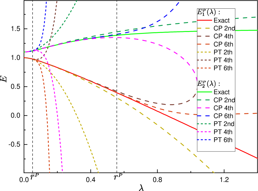
Figure 1: Results of $E_{1}^{{}_{P}}(\lambda)$ and $E_{2}^{{}_{P}}(\lambda)$ calculated respectively by characteristic polynomial (CP) for different-order (2nd, 4th and 6th) $\lambda$-expansion of coefficients, and by different-order (2nd, 4th and 6th) perturbation theory (PT), for the example model. Also shown is the exact value of $E_{1}^{{}_{P}}(\lambda)$ and $E_{2}^{{}_{P}}(\lambda)$. The position of $\lambda=\bar{r}^{{}_{P}}$ and $r^{{}_{P}}$ has been marked by vertical dash lines.

An interesting thing should be noted is that in our calculation of the characteristic polynomial, ISP terms always cancel in the coefficients $P_{1}(\lambda)$ and $P_{2}(\lambda)$, no matter for 2nd, 4th or 6th order $\lambda$-expansion, leading to a final result being free from the ISP.

Furthermore, as far as our simple example ($N=2$) is concerned, the branch points of $E_{1}^{{}_{P}}(\lambda)$ and $E_{2}^{{}_{P}}(\lambda)$ lying nearest to the origin can be alternatively determined by $P_{1}(\lambda)^{2}-4P_{2}(\lambda)=0$, i.e., by the condition for $E_{1}^{{}_{P}}(\lambda)=E_{2}^{{}_{P}}(\lambda)$ from Eq. (9). When we retain terms in $P_{1}(\lambda)$ and $P_{2}(\lambda)$ to the order of $\lambda^{2}$, $\lambda^{4}$, $\lambda^{6}$, such branch points are obtained as $\pm 0.0513922i$, $\pm 0.0513924i$, $\pm 0.0513922i$, respectively, of which the difference is vanish small. These values are in good agreement with the exact one $\pm 0.051392i$ obtained above.

4 Discussion

One advantage of using characteristic polynomial is its uniqueness. There are infinitely many similar matrices that can be chosen as $H_{\mathrm{eff}}(\lambda)$; of which, the convergence radii for $\lambda$-expansion obviously can be different, but all should not exceed that of the characteristic-polynomial coefficients $P_{n}(\lambda)$, i.e., $r^{{}_{P}}$. Mathematically, the most convergent form of $H_{\mathrm{eff}}(\lambda)$ can be obtained via the least action of the unitary transformation to block diagonalize $H(\lambda)$, i.e., via changing $H(\lambda)$ as little as possible to bring it into a block diagonal form [9]. Such “least action” condition generally is hard to be satisfied. Hence, one may expect that it is difficult to construct an $H_{\mathrm{eff}}(\lambda)$ which has the same convergence radius for $\lambda$-expansion as $r^{{}_{P}}$. Actually, it has been shown that the convergence radii of $\lambda$-series expansion for those $H_{\mathrm{eff}}(\lambda)$ constructed by methods such as Rayleigh-Schrödinger or Brillouin-Wigner perturbation are mainly determined by the smallest module of the so-called “exceptional points” in the complex plane of $\lambda$ [1, 20], where some $P$- and $Q$-state eigenvalues, say $E_{1}^{{}_{P}}(\lambda)$ and $E_{1}^{{}_{Q}}(\lambda)$, coincide. These points should be distinguished from the branch points, since they become the same only if the associated eigenfunctions also coincide [10, 20]. Obviously, each branch point must also be an exceptional point, but the reverse is not necessarily true. This means that for those $H_{\mathrm{eff}}(\lambda)$, the convergence radius of $\lambda$-expansion indeed cannot exceed $r^{{}_{P}}$.

It is interesting whether there exists some unified way to construct $H_{\mathrm{eff}}(\lambda)$ so that its convergence radius for $\lambda$-expansion is always equal to $r^{{}_{P}}$. The answer is yes. In fact, we can construct an effective Hamiltonian directly using the characteristic-polynomial coefficients $P_{n}(\lambda)$ as follows

$$\bar{H}_{\mathrm{eff}}(\lambda)=\begin{bmatrix}\bar{P}_{1}(\lambda)&\bar{P}_{2}(\lambda)&\cdots&\bar{P}_{N-1}(\lambda)&\bar{P}_{N}(\lambda)\\ 1&0&\cdots&0&0\\ 0&1&\cdots&0&0\\ \vdots&\vdots&\ddots&\vdots&\vdots\\ 0&0&\cdots&1&0\end{bmatrix},$$ (13)

where $\bar{P}_{n}(\lambda)\equiv(-1)^{n+1}P_{n}(\lambda)$. One can easily verify that the characteristic polynomial of $\bar{H}_{\mathrm{eff}}(\lambda)$ is just in the same form shown in Eq. (5) [21, 22], and hence it indeed can be viewed an effective Hamiltonian. Obviously, due to its relationship with $P_{n}(\lambda)$, $\bar{H}_{\mathrm{eff}}(\lambda)$ must have a convergence radius same as $r^{{}_{P}}$ for $\lambda$-expansion.

Another point we want to discuss is whether our calculation of $P_{n}(\lambda)$ and $\det[E-H_{\mathrm{eff}}(\lambda)]$ can apply to the case with degenerate or nearly-degenerate $\epsilon_{n}^{{}_{P}}$. In the simple example above, we have already mentioned that in finite-order calculation of $P_{n}(\lambda)$, ISP terms tend to cancel. It is interesting whether this cancellation still occurs when the order is very large or even tends to infinity, since as shown in Eqs (2.1)–(2.N), the $E^{{}_{P}}_{n}(\lambda)$-series used to calculate $P_{n}(\lambda)$ always have such terms .

We note that, due to the uniqueness of characteristic polynomial, if one can construct any effective Hamiltonian $H_{\mathrm{eff}}(\lambda)$ which can be expanded in powers of $\lambda$ without the appearance of ISP terms, regardless of the convergence radius, the complete cancellation of these terms in the $\lambda$-expansion of $\det[E-H_{\mathrm{eff}}(\lambda)]$ or $P_{n}(\lambda)$ can be proved.

Actually, the expanded form of $H_{\mathrm{eff}}(\lambda)$ constructed in usual ways always does not have ISP terms, at least when the first few orders of $\lambda$-expansion are retained [1, 2, 3, 4, 5, 6, 7]. A form of $H_{\mathrm{eff}}(\lambda)$ which does not have any ISP terms for all orders of $\lambda$-expansion is constructed in the Appendix.

Then, we find that ISP terms indeed are canceled completely in the $\lambda$-expansion of $\det[E-H_{\mathrm{eff}}(\lambda)]$ or $P_{n}(\lambda)$. This means that although non-degenerate unperturbed energies have been assumed for $P$-space states, our discussion is free from the ISP, and can directly apply to the cases with these energies being nearly-degenerate or degenerate. Hence, our discussion of the characteristic polynomial of $H_{\mathrm{eff}}(\lambda)$ may find its potential use in MRPT in quantum chemistry or other effective-Hamiltonian problems.

5 Conclusion

In conclusion, we have discussed the properties of the characteristic polynomial of $H_{\mathrm{eff}}(\lambda)$ for a general model Hamiltonian. Unlike $P$-space energy eigenvalues, $\det[E-H_{\mathrm{eff}}(\lambda)]$ and the coefficients $P_{n}(\lambda)$ do not have the branch points due to the $PP$-crossing, and hence are more suitable for a perturbation calculation. We can calculate $P_{n}(\lambda)$, and hence $\det[E-H_{\mathrm{eff}}(\lambda)]$ in a perturbative way, which can be further used to solve for the eigenvalues $E^{{}_{P}}_{n}(\lambda)$. Such procedure generally possesses a larger convergence radius for $\lambda$ expansion, comparing with the direct perturbation calculation of $E^{{}_{P}}_{n}(\lambda)$. An effective Hamiltonian $\bar{H}_{\mathrm{eff}}(\lambda)$, which has the same branch points and convergence radius for $\lambda$ expansion as our characteristic polynomial, has also been constructed.

The uniqueness of $\det[E-H_{\mathrm{eff}}(\lambda)]$ also brings convenience to our discussion. We find that our procedure is free from the ISP which arises when the unperturbed energies of $P$-space states become nearly-degenerate or degenerate, as frequently encountered in cases such as the MRPT study of multiconfigurational quantum-chemical systems. Due to this advantage, one can expect that our treatment of $\det[E-H_{\mathrm{eff}}(\lambda)]$ may find more potential use in the future study of effective-Hamiltonian problems.

Appendix A Constructing an effective Hamiltonian without the appearance of ISP terms

To construct an effective Hamiltonian without any ISP terms for our $H(\lambda)$, we follow the procedure in Refs. [2, 23, 24]. We can denote the eigenstate associated with $E_{n}^{{}_{P}}(\lambda)$ by $\left|\Psi_{n}\right\rangle$, i.e.,

$$H(\lambda)\left|\Psi_{n}\right\rangle=E_{n}^{{}_{P}}(\lambda)\left|\Psi_{n}\right\rangle,\quad n=1,\ldots,N.$$

We let $\hat{P}\equiv\sum_{n}|\psi^{{}_{P}}_{n}\rangle\langle\psi^{{}_{P}}_{n}|$ and introduce

$$|\Psi^{{}_{P}}_{n}\rangle\equiv\hat{P}\left|\Psi_{n}\right\rangle,$$

where $|\Psi^{{}_{P}}_{n}\rangle$ is required to be normalized, but $\left|\Psi_{n}\right\rangle$ is not. One can further introduce the so-called wave operator $\hat{\Omega}$ by requiring that,

$$|\Psi_{n}\rangle=\hat{\Omega}\left|\Psi^{{}_{P}}_{n}\right\rangle.$$

It has been shown that $\hat{\Omega}\hat{P}=\hat{\Omega}$ and $\hat{P}\hat{\Omega}=\hat{P}$, from which we have

$$\langle\psi^{{}_{P}}_{m}|\hat{\Omega}|\psi^{{}_{P}}_{n}\rangle=\langle\psi^{{}_{P}}_{m}|\hat{P}\hat{\Omega}|\psi^{{}_{P}}_{n}\rangle=\langle\psi^{{}_{P}}_{m}|\hat{P}|\psi^{{}_{P}}_{n}\rangle=\delta_{n,m},$$ (14)

$$\langle\psi^{{}_{P(Q)}}_{m}|\hat{\Omega}|\psi^{{}_{Q}}_{n}\rangle=\langle\psi^{{}_{P(Q)}}_{m}|\hat{\Omega}\hat{P}|\psi^{{}_{Q}}_{n}\rangle=0.$$ (15)

An effective Hamiltonian can then be constructed as

$$H_{\mathrm{eff}}(\lambda)=\hat{P}H_{0}\hat{P}+\lambda\hat{P}H_{I}\hat{\Omega}\\ =\hat{P}H_{0}\hat{P}+\lambda\hat{P}H_{I}(\hat{\Omega}^{(0)}+\hat{\Omega}^{(1)}+\hat{\Omega}^{(2)}+\cdots)$$ (16)

where $\hat{\Omega}$ has be expanded in powers of $\lambda$ as $\hat{\Omega}=\hat{\Omega}^{(0)}+\hat{\Omega}^{(1)}+\hat{\Omega}^{(2)}+\cdots$, with $\Omega^{(k)}$ standing for the $k$th order term. Obviously, $\hat{\Omega}^{(0)}=\hat{P}$.

One can further derive an equation for $\hat{\Omega}$,

$$\left[\hat{\Omega},H_{0}\right]=\lambda H_{I}\hat{\Omega}-\lambda\hat{\Omega}\hat{P}H_{I}\hat{\Omega},$$

with which an iterative formula for $\hat{\Omega}^{(k)}$ can be derived:

$$\left[\hat{\Omega}^{(k)},H_{0}\right]=\hat{A}_{k}\equiv\lambda H_{I}\hat{\Omega}^{(k-1)}-\lambda\sum_{j=0}^{k-1}\hat{\Omega}^{(j)}\hat{P}H_{I}\hat{\Omega}^{(k-j-1)},$$ (17)

where $k=1,2,\cdots$.

We can calculate $\hat{\Omega}^{(k)}$ in the bases of $\{|\psi^{{}_{P}}_{n}\rangle,|\psi^{{}_{Q}}_{m}\rangle\}$. Due to Eqs. (14) and (15), the nonzero matrix elements of $\hat{\Omega}^{(k)}$ ($n\geq 1$) can only be those such as $\langle\psi^{{}_{Q}}_{m}|\hat{\Omega}^{(k)}|\psi^{{}_{P}}_{n}\rangle$.

Now, we show that ISP terms, i.e., these containing “$\frac{1}{\epsilon_{n_{1}}^{{}_{P}}-\epsilon_{n_{2}}^{{}_{P}}}$”, would not appear in the $H_{\mathrm{eff}}(\lambda)$ constructed above. Actually, all our procedure till now can be found in Refs. [2, 23, 24]. Noting that $\langle\psi^{{}_{Q}}_{m}|[\hat{\Omega}^{(k)},H_{0}]|\psi^{{}_{P}}_{n}\rangle=(\epsilon_{n}^{{}_{P}}-\epsilon_{m}^{{}_{Q}})\langle\psi^{{}_{Q}}_{m}|\hat{\Omega}^{(k)}|\psi^{{}_{P}}_{n}\rangle$, we have

$$\langle\psi^{{}_{Q}}_{m}|\hat{\Omega}^{(k)}|\psi^{{}_{P}}_{n}\rangle=\frac{\langle\psi^{{}_{Q}}_{m}|\hat{A}_{k}|\psi^{{}_{P}}_{n}\rangle}{\epsilon_{n}^{{}_{P}}-\epsilon_{m}^{{}_{Q}}},$$

from which, it follows that if $\langle\psi^{{}_{Q}}_{m}|\hat{A}_{k}|\psi^{{}_{P}}_{n}\rangle$, or equivalently, the matrix elements of $\hat{\Omega}^{(j)}$, ($j=0,1,\cdots,k-1$), do not contain any ISP terms, neither does $\langle\psi^{{}_{Q}}_{n}|\hat{\Omega}^{(k)}|\psi^{{}_{P}}_{m}\rangle$.

Noting that ISP terms do not appear in $\hat{\Omega}^{(0)}=\hat{P}$, we conclude that $\hat{\Omega}^{(1)}$, and hence $\hat{\Omega}^{(2)},\hat{\Omega}^{(3)},\cdots$, all would not have any ISP terms appear in their matrix elements. Hence, when being expanded in powers of $\lambda$, the $H_{\mathrm{eff}}(\lambda)$ given by Eq. (16) indeed is an effective Hamiltonian without any ISP terms.

References

[1] T. H. Schucan and H. A. Weidenmüller, Ann. Phys. 73 (1972) 108; 76 (1973) 483.
[2] K. Takayanagi, Ann. Phys. 364 (2016) 200; 415 (2020) 168119.
[3] E. Magesan and J. M. Gambetta, Phys. Rev. A 101 (2020) 052308.
[4] P.J. Ellis and E. Osnes, Rev. Mod. Phys. 49 (1977) 777.
[5] K. Suzuki, Prog. Theor. Phys. 68 (1982) 246.
[6] J. R. Schrieffer and P. A. Wolff, Phys. Rev. 149 (1966) 491.
[7] A. H. MacDonald, S. M. Girvin and D. Yoshioka, 37 (1988) 9753.
[8] C. E. Soliverez, Phys. Rev. A 24 (1981) 4.
[9] L. S. Cederbaum, J. Schirmer and H-D. Meyer, J. Phys. A: Math. Gen. 22 (1989) 2427.
[10] A. R. Forsyth, Theory of Functions of a Complex Variable, Cambridge University, Cambridge,
1893.
[11] K. Knopp, Theory of Functions II, Dover, New York, 1947.
[12] L.V. Ahlfors, Complex Analysis, McGraw-Hill, New York,
1966.
[13] Y. -K. Choe, H. A. Witek, J. P. Finley and K. Hirao, J. Chem. Phys. 114 (2001) 3913.
[14] H. A. Witek, Y. -K. Choe, J. P. Finley and K. Hirao, J. Comput. Chem. 23 (2002) 957.
[15] F. A. Evangelista, J. Chem. Phys. 149 (2018) 030901.
[16] F. Pawłowski, J. Olsen and P. Jørgensen, J. Chem. Phys. 150 (2019) 134111.
[17] Y. Guo, K. Sivalingam and F. Neese, J. Chem. Phys. 154 (2021) 214111.
[18] W. D. Heiss and W.-H. Steeb, J. Math. Phys. 32 (1991) 3003.
[19] W.-H. Steeb and W. D. Heiss, Phys. Lett. A 152 (1991) 339; Phys. Scr. 47 (1993) 321.
[20] T. Kato, Perturbation Theory of Linear Operators, Springer,
New York, 1966.
[21] W. H. Press, S. A. Teukolsky, W. T. Vetterling, B. P. Flannery, Numerical Recipes
in Fortran 77, Cambridge University Press, New York, 1992.
[22] L. W. Johnson, and R. D. Riess, Numerical Analysis, MA: Addison-Wesley, Reading, 1982.
[23] I. Lindgren, J. Phys. B: At. Mol. Phys. 7 (1974) 2441.
[24] I. Lindgren, J. Morrison, Atomic Many-Body Theory, Springer, Berlin,
1986.