A mean-field game of market-making against strategic traders

Abstract

We design a market-making model à la Avellaneda and Stoikov in which the market-takers act strategically, in the sense that they design their trading strategy based on an exogenous trading signal. The market-maker chooses her quotes based on the average market-takers’ behaviour, modelled through a mean-field interaction. We derive, up to the resolution of a coupled HJB–Fokker–Planck system, the optimal controls of the market-maker and the representative market-taker. This approach is flexible enough to incorporate different behaviours for the market-takers and takes into account the impact of their strategies on the price process.

Keywords: market-making, algorithmic trading, mean-field games

1 Introduction

On financial markets, a market-maker is usually defined as a liquidity provider. In a nutshell, it is a market participant who provides bid and ask (i.e. buy and sell) prices on one or several assets. The market-maker makes profit by earning the price difference between her buy and sell orders, called the bid–ask spread. She faces the following optimisation problem: being rarely executed at a very high spread, or being often executed at a very low spread. In the first case, the marked-to-market gain will be high, and conversely in the second case. On most of the order-driven markets, such as equities, the market-making activity is provided by a small number of high-frequency trading firms which are the counterpart of the vast majority of the transactions, see for example Megarbane, Saliba, Lehalle, and Rosenbaum [42]. They quote almost continuously bid and ask prices at the best limits, and their strategies are mostly based on either their superior proprietary technology, or on arbitrage strategies on cross-listed securities based on microstructure signals, see for instance Baldacci and Manziuk [3]. On quote-driven markets, such as for many fixed income products and single stock options, the liquidity-takers, who have a fair price in mind, first request a price for a given transaction size of the asset to a market-maker, often called dealer. The dealer answers by providing a price for the corresponding size, which is then accepted or rejected by the client. It is common that, similarly to order-driven markets, a small number of dealers provide the vast majority of liquidity to a large set of clients. On some specific products, such as options on single stocks, there can even be a monopolistic situation where there is a single liquidity provider.

The optimal market-making problem has been the subject of a vast academic literature. Seminal references are Grossman and Miller [29], and Ho and Stoll [33]. In particular, the authors of [33] studied the behaviour of a market-maker confronting a stochastic demand, using stochastic control theory. This framework has inspired the well-known model of Avellaneda and Stoikov [2], which was designed to be applicable to order-driven market at the high-frequency scale. However, due to the continuous nature of the market-maker’s spreads, and the assumption that the underlying asset is a diffusion process, this model turned out to also be suitable for quote-driven markets, such as corporate bonds markets. By providing a rigorous analysis of the stochastic control problem of [2], Guéant, Lehalle, and Fernandez-Tapia [31] showed, in the case of a CARA utility function, that the market-maker’s problem boiled down to a system of linear ordinary differential equations. More recent contributions to the market-making literature can be found in the works of Cartea, Jaimungal, and Penalva [19], Cartea and Jaimungal [18], or Cartea, Donnelly, and Jaimungal [20, 21], who enriched the initial model by introducing $\displaystyle\alpha$ signals, ambiguity aversion, competition with other agents… In all these articles, the authors consider a risk-adjusted expectation instead of a CARA utility function, which leads to the same optimal quotes with a suitable transformation of the intensity functions, see Manziuk [41]. More recently, multi-asset market-making has been addressed through reinforcement learning, see Guéant and Manziuk [30], and dimensionality reduction techniques, see Bergault and Guéant [10], Bergault, Evangelista, Guéant, and Vieira [11], or Baldacci, Bergault, and Guéant [5] for the special case of option market-making. All these models are well-suited for OTC markets and for order-driven markets in the case of small tick assets, but are not straightforwardly applicable to design market-making strategies on order books with a large tick size, where the control process lies in a discrete tick grid. One of the main contributions to this literature is Guilbaud and Pham [32], where the authors build a model where a market-maker can send both limit and market orders on the order book of a single asset. In a similar vein, the model with uncertainty zones introduced by Robert and Rosenbaum [43] to reproduce accurately the high-frequency behaviour of an asset, has been incorporated into a market-making model, see Baldacci, Bergault, Derchu, and Rosenbaum [4].

A striking feature of all the aforementioned models is that the market-takers are systematically assumed to be passive, in the sense that they only respond to a quote proposed by the market-maker through the intensity of a point process. The case of market-making with competitive agents has rarely been addressed in the literature. The reason is that accounting for multiple agents leads to high dimensional problems with complicated interactions, and typically renders the analysis intractable using standard numerical methods in stochastic optimal control. In the context of optimal trading, interactions between a large number of agents have been modelled through the use of mean-field games. This is one possible solution to model more complex market interactions, because of its tractability compared to multi-agent models. The classical optimal execution problem à la Almgren and Chriss [1] is thus addressed by controlling McKean–Vlasov equations in Cardaliaguet and Lehalle [13]: the trader faces uncertainty with respect to price changes because of his actions but also has to deal with price changes due to other similar market participants, impacting the prices permanently and acting strategically. Therefore, the distribution of the controls appears inside the drift of the asset’s price process. In Huang, Jaimungal, and Nourian [38], the authors extend the previous work on optimal trading using a major–minor mean-field game framework, where a major agent is liquidating a large portion of shares, and a large number of minor agents trade along with the major agent. Mean-field games have also been applied by Casgrain and Jaimungal [22, 23] to the case of heterogeneous traders who aim at performing optimal execution. All these models have in common that the mean-field interaction is through the drift of the asset’s price process. Moreover, in the case of major–minor optimal trading in Huang, Jaimungal, and Nourian [38], both the major and the minor agents are traders who only differ by their influence on the market. As stated previously, there is no strategic market-takers in the extensions of Avellaneda and Stoikov [2] due to the difficulties in modelling the interactions between the market-maker and several market-takers. Having a very granular model will lead to a high-dimensional stochastic control problems, intractable with standard numerical methods. Therefore, we propose in this paper to employ a major–minor mean-field game where the market-maker plays the role of the major player, whereas the strategic market-takers are modelled through a mean-field of minor agents.

We emphasise that many recent papers also make use of the theory of mean-field games with a major player, introduced and studied deeply by Buckdahn, Li, and Peng [12], Cardaliaguet, Cirant, and Porretta [14], Carmona and Wang [15, 16], Carmona and Zhu [17], and Lasry and Lions [39]. As in standard mean-field games and optimal control theory, linear–quadratic problems are of particular interest in the presence of a major player facing a mean-field of minor agents as they generally boil down to a system of ODEs of the Riccati type, that can sometimes be solved explicitly. Those problems have been studied in particular in Huang [35, 36], Huang, Wang, and Wu [34], Huang and Nguyen [37], but also in Firoozi and Caines [27, 26] and Firoozi, Jaimungal, and Caines [28].

Coming back to the present paper, our main goal is to address the problem of a market-maker providing the vast majority of the liquidity on an underlying asset. The market-maker faces a very high number of traders, or market-takers, with possibly different behaviours such as momentum or mean reverting strategies. Each market-taker acts strategically in the sense that they send request to the market-maker with a fair price in mind, which results from their own optimisation, depending on their inventory and their trading signal. The market-maker proposes quotes based on her inventory process, and the behaviour of her counterparts, which are aggregated through a mean-field game. The problem thus takes the form of a mean-field game with controlled jumps: the intensities of the order arrivals of all market participants are averaged through a single point process, and the market-maker increases her execution rate if her quote is close to the fair price resulting from the mean-field equilibrium of the minor players. Based on the mean-field equilibrium between the traders, the market-maker computes the average fair price of the mean-field. If the fair bid price of the minor players is higher than her ask quote, for instance, the intensity of arrival orders at the ask for the market-maker will decrease and conversely. We characterise completely the problem by a system of Fokker–Planck equations for the mean-field game associated to the minor players, and a (decoupled) HJB equation for the major player, which can be efficiently solved via classic numerical methods on grids. Up to the resolution of these PDEs, we derive the optimal strategies of both the representative market-taker, and the market-maker. To the best of our knowledge, this is the first work on optimal market-making taking into account the strategic behaviour of market-takers. We believe that the use of mean-field games to represent the interaction between market-maker and market-takers can lead to substantial improvement of the usual optimal market-making models, without increasing drastically the numerical complexity. The numerical results with a set of reasonable market parameters exhibit some interesting features. The probability distribution of the market-takers’ inventory shifts with the exogenous trading signal and the market-maker’s strategy is adjusted with respect to this flow. Even with an empty inventory, the market-takers prefer to have a non-zero signal as it will allow them to make more profit over the trading horizon: the worst-case for a market-taker is a flat signal. Moreover, when market-takers have a very volatile signal, the distribution of inventories remains symmetric around $\displaystyle 0$ but with two ‘bumps’ representing their incapacity to react rapidly to a change of signal. These results enable to enhance the seminal work of Avellaneda and Stoikov [2] in the sense that the behaviour of market-takers is not fixed as a function of the quotes of the market-maker only, but as a function of their own view on the price process as well as their current inventory. This is of particular importance as it leads to a more accurate estimation of the PnL of the strategy of the market-maker. Moreover, our model also provides the optimal strategy of an informed market-taker, which is absent in Avellaneda and Stoikov [2].

The article is constructed as follows: in Section 2, we introduce informally an $\displaystyle N$-player version of the model, which justifies the presentation in Section 3 of the mean-field probabilistic framework. In Section 4, we solve those problems in the case of Markovian controls, while Section 5 is devoted to the numerical results.

Notations: Let $\displaystyle\mathbb{N}^{\star}$ be the set of all positive integers. For any $\displaystyle(\ell,c)\in\mathbb{N}^{\star}\times\mathbb{N}^{\star}$, $\displaystyle\mathcal{M}_{\ell,c}(\mathbb{R})$ will denote the space of $\displaystyle\ell\times c$ matrices with real entries. Elements of the matrix $\displaystyle M\in\mathcal{M}_{\ell,c}(\mathbb{R})$ are denoted by $\displaystyle(M^{i,j})_{(i,j)\in\{1,\dots,\ell\}\times\{1,\dots,c\}}$ and the transpose of $\displaystyle M$ is denoted by $\displaystyle M^{\top}$. We identify $\displaystyle\mathcal{M}_{\ell,1}$ with $\displaystyle\mathbb{R}^{\ell}$. When $\displaystyle\ell=c$, we let $\displaystyle\mathcal{M}_{\ell}(\mathbb{R}):=\mathcal{M}_{\ell,\ell}(\mathbb{R})$. For any $\displaystyle x\in\mathcal{M}_{\ell,c}(\mathbb{R})$, and for any $\displaystyle j\in\{1,\dots,c\}$, $\displaystyle x^{j}\in\mathbb{R}^{\ell}$ is the $\displaystyle j$-th column of $\displaystyle M$. Moreover, for any $\displaystyle x\in\mathcal{M}_{\ell,c}(\mathbb{R})$ and any $\displaystyle j\in\{1,\dots,c\}$, $\displaystyle x^{-j}\in\mathcal{M}_{\ell,c-1}(\mathbb{R})$ denotes the matrix $\displaystyle x$ without the $\displaystyle j$-th column. For a pair $\displaystyle(x^{0},x)\in\mathbb{R}^{\ell}\times\mathcal{M}_{\ell,c}(\mathbb{R})$, we denote by $\displaystyle x^{-0}$ the matrix $\displaystyle x^{-0}:=x$. For any $\displaystyle x\in\mathcal{M}_{\ell,c}(\mathbb{R})$ and $\displaystyle y\in\mathbb{R}^{\ell}$, we also define for $\displaystyle i\in\{1,\dots,\ell\}$, $\displaystyle y\otimes_{i}x\in\mathcal{M}_{\ell,c+1}(\mathbb{R})$ as the matrix whose first $\displaystyle i-1$ columns are equal to the first $\displaystyle i-1$ columns of $\displaystyle x$, such that for $\displaystyle j\in\{i+1,\dots,c+1\}$, its $\displaystyle j$-th column is equal to the $\displaystyle(j-1)$-th column of $\displaystyle x$, and whose $\displaystyle i$-th column is equal to $\displaystyle y$. We extend naturally this definition to $\displaystyle\mathcal{M}_{\ell,c}(\mathbb{R})$-valued processes. For $\displaystyle(a,b)\in\mathbb{R}^{2}$ with $\displaystyle a\leq b$, we denote $\displaystyle\llbracket a,b\rrbracket:=[a,b]\cap\mathbb{Z}$. For a generic finite-dimensional Euclidean space $\displaystyle E$, a generic filtered probability space $\displaystyle({\cal A},{\cal G},\mathbb{G},\Pi)$, we let $\displaystyle\mathbb{L}^{0}(E,\mathbb{G})$ be the space of $\displaystyle E$-valued, $\displaystyle\mathbb{G}$-predictable processes.

2 Some motivation: one market-maker facing several market-takers

In this section, we provide motivations for the use of mean-field games to model the interaction between a market-maker and a large number of informed market-takers. We first begin by describing the problem of $\displaystyle N$ market-takers facing one market-maker. Since the purpose of this section is purely motivational, we adopt a heuristic approach in the presentation, and avoid properly defining the weak formulation of the problem, which we reserve to the mean-field version in Section 3.1.

2.1 Framework

We consider a trading horizon $\displaystyle T>0$ and a filtered probability space $\displaystyle\big{(}\Omega,\mathcal{F},\mathbb{F}:=(\mathcal{F}_{t})_{t\in[0,T]},\mathbb{P}\big{)}$ under which all the stochastic processes are defined. We set some positive integer $\displaystyle N\in\mathbb{N}^{\star}$, corresponding to the number of informed market-takers acting on a market consisting of a single asset whose price process is denoted by $\displaystyle S.$ This quantity, whose definition will be detailed later, can be thought as the mid-price of the asset which can be impacted by the trading activity of the market-takers.

We consider a market whose functioning is as follows: for any $\displaystyle i\in\{1,\dots,N\}$, at time $\displaystyle t\in[0,T]$, the $\displaystyle i$-th trader has a fair buy or sell price in mind, around the mid-price $\displaystyle S_{t}$, meaning that he is ready to buy or sell the asset at time $\displaystyle t$ at prices respectively given by

$$P^{b}(S_{t},\delta^{i,b}_{t}):=S_{t}-\delta^{i,b}_{t},\;\text{\rm and}\;P^{a}(S_{t},\delta_{t}^{i,a}):=S_{t}+\delta^{i,a}_{t},$$

where for $\displaystyle i\in\{1,\dots,N\}$, $\displaystyle\big{(}\delta^{i,b},\delta^{i,a}\big{)}$ are what we call the control processes of the $\displaystyle i$-th trader. The $\displaystyle i$-th trader can trade with any participant of the market. His number of filled bid and ask orders are modelled by counting processes $\displaystyle N^{i,b}$ and $\displaystyle N^{i,a}$, with intensities respectively given by $\displaystyle\lambda^{i,b,\delta^{i}}:=\Lambda^{m}(\delta^{i,b})$ and $\displaystyle\lambda^{i,a,\delta^{i}}:=\Lambda^{m}(\delta^{i,a})$, where

$$\displaystyle\Lambda^{m}(x):=A^{m}\exp\bigg{(}-\frac{k^{m}}{\sigma}x\bigg{)},\;x\in\mathbb{R}.$$ (2.1)

The form of the intensities deserves several comments, which hold for any $\displaystyle i\in\{1,\dots,N\}$

• the coefficient $\displaystyle A^{m}>0$ is the average number of transactions by unit of time when the $\displaystyle i$-th market-takers’ fair price is identically equal to the mid-price;

• the coefficient $\displaystyle k^{m}>0$ represents the sensitivity of the intensity to the mid-to-bid and ask-to-mid quotes proposed by the $\displaystyle i$-th market-taker. More precisely, the market-taker trades frequently at the bid (resp. at the ask) when his mid-to-bid (resp. ask-to-mid) price is relatively small;

• the intensities are decreasing functions of the volatility of the asset $\displaystyle\sigma>0$, defined below, meaning that a high volatility induces a lower number of trades and conversely, see for example Dayri and Rosenbaum [24], Madhavan, Richardson, and Roomans [40], or Wyart, Bouchaud, Kockelkoren, Potters, and Vettorazzo [44].

At any time $\displaystyle t\in[0,T]$, the market-maker, who does not know the fair prices of the market-takers, proposes quotes around the mid-price $\displaystyle S_{t}$ at which she is ready to buy or sell the asset to the $\displaystyle i$-th trader. For $\displaystyle t\in[0,T]$, these prices are

$$\displaystyle P^{b}(S_{t},\delta_{t}^{0,b}):=S_{t}-\delta_{t}^{0,b},\;\text{\rm and}\;P^{a}(S_{t},\delta_{t}^{0,a}):=S_{t}+\delta_{t}^{0,a},\;t\in[0,T],$$

where $\displaystyle(\delta^{0,b},\delta^{0,a})$ are what we call the control processes of the market-maker. The set of admissible controls for the $\displaystyle N+1$ players is defined as

$$\displaystyle\mathcal{A}_{N}=\Big{\{}(\delta^{0},\delta^{-0})=\big{(}(\delta^{0,b},\delta^{0,a}),(\delta^{i,b},\delta^{i,a})_{i\in\{1,\dots,N\}}\big{)}\in\mathbb{L}^{0}\big{(}{\cal M}_{2,N+1}(\mathbb{R}),\mathbb{F}\big{)}:(\delta^{0},\delta^{-0})\;\text{\rm bounded by}\;\delta_{\infty}\Big{\}},$$

for a given $\displaystyle\delta_{\infty}>0$. The optimisation problem of the $\displaystyle i$-th market-taker is a function of the spread vector $\displaystyle\delta^{-i}$ quoted by the $\displaystyle N-1$ other market-takers and the spread $\displaystyle\delta^{0}$ of the market-maker. Hence, each market-taker will maximise his PnL given the actions of the other market-takers to obtain his so-called best-reaction function. We define the set of admissible controls of the $\displaystyle i$-th player given controls $\displaystyle\delta^{0}$ and $\displaystyle\delta^{-i}$ chosen by the other market participants by

$$\displaystyle\mathcal{A}_{N}^{i}(\delta^{0},\delta^{-i}):=\Big{\{}\delta\in\mathbb{L}^{0}\big{(}\mathcal{M}_{2,1}(\mathbb{R}),\mathbb{F}\big{)}:(\delta^{0},\delta\otimes_{i}\delta^{-i})\in\mathcal{A}_{N}\Big{\}},$$

and the set of admissible controls of the market-maker given a control $\displaystyle\delta^{-0}$ played by other market participants

$$\displaystyle\mathcal{A}_{N}^{0}(\delta^{-0})=\Big{\{}\delta\in\mathbb{L}^{0}\big{(}\mathcal{M}_{2,1}(\mathbb{R}),\mathbb{F}\big{)}:(\delta,\delta^{-0})\in\mathcal{A}_{N}\Big{\}}.$$

The number of transactions at the bid and at the ask for the market-maker is modelled by two processes $\displaystyle N^{0,b}$ and $\displaystyle N^{0,a}$, with intensity processes $\displaystyle\lambda^{0,b,\delta}$ and $\displaystyle\lambda^{0,a,\delta}$, respectively given by

$$\lambda^{0,b,\delta}_{t}:=\Lambda\bigg{(}\frac{1}{N}\sum_{i=1}^{N}\delta_{t}^{i,a},\delta_{t}^{0,b}\bigg{)},\;\text{and}\;\lambda^{0,a,\delta}_{t}:=\Lambda\bigg{(}\frac{1}{N}\sum_{i=1}^{N}\delta_{t}^{i,b},\delta_{t}^{0,a}\bigg{)},\;\forall t\in[0,T],$$

where

$$\displaystyle\Lambda(x,y):=A\exp\bigg{(}-\frac{k}{\sigma}(x+y)\bigg{)},\;(x,y)\in\mathbb{R}^{2},$$ (2.2)

for positive constants $\displaystyle A$ and $\displaystyle k$. Hence, these intensities depend on the difference between the average fair price of the market-takers on the one hand, and the price proposed by the market-maker on the other hand: for instance, if the average fair price at which market-makers are ready to sell the asset is very large compared to the price at which the market-maker is ready to buy, the market-maker will not trade often. In a framework where all the processes $\displaystyle(\delta^{i,b},\delta^{i,a})$ are constant equal to zero, that is for all $\displaystyle t\in[0,T],\delta_{t}^{i,a}=\delta_{t}^{i,b}=0$, the market-takers are considered as ‘passive’, and we recover the classical optimal market-making framework of Avellaneda and Stoikov [2], Cartea, Jaimungal, and Penalva [19], and Guéant, Lehalle, and Fernandez-Tapia [31].

The dynamics of the price process $\displaystyle S$ under which the market-maker and the $\displaystyle N$ market-takers compute the marked-to-market value of their inventory is defined as

$$\displaystyle\mathrm{d}S_{t}=\sigma\mathrm{d}W_{t}+\frac{\kappa}{N}\sum_{i=1}^{N}\big{(}\mathrm{d}N^{i,b}_{t}-\mathrm{d}N^{i,a}_{t}\big{)},$$ (2.3)

where $\displaystyle\kappa$ and $\displaystyle\sigma$ are positive constants, $\displaystyle W$ is a one-dimensional Brownian motion, independent of $\displaystyle N^{0,b}$ and $\displaystyle N^{0,a}$. This equation deserves several comments

• $\displaystyle\sigma W$ represents the diffusion part of the asset’s price, independent from the trading activity;

• the asset price is impacted by the average behaviour of the market-takers, through the so-called permanent market impact effect: when, on average, market-takers buy (resp. sell) the asset at a high rate, its price increases (resp. decreases).

Finally, we assume that each market-taker reacts to a specific signal on the price, modelled for the $\displaystyle i$-th market-taker, for any $\displaystyle i\in\{1,\dots,N\}$, by a process $\displaystyle b^{i}$, verifying

$$b^{i}_{t}:=N_{t}^{i,+}-N_{t}^{i,-},\;t\in[0,T],$$

where $\displaystyle N^{i,+}$ and $\displaystyle N^{i,-}$ are Poisson processes of intensities $\displaystyle\bar{\lambda}^{+}$ and $\displaystyle\bar{\lambda}^{-}$, independent of $\displaystyle(W,N^{0,b},N^{0,a},N^{i,b},N^{i,a})$. This signal process corresponds to the belief of the $\displaystyle i$-th market-taker concerning the drift of the asset, which can be modified by the information he acquires over time.

2.2 The problem of the market-maker

The cash process $\displaystyle X^{0}$ of the market-maker is naturally defined as follows

$$\displaystyle X^{0}_{t}:=X^{0}_{0}+\int_{0}^{t}P^{a}(S_{s},\delta_{s}^{0,a})\mathrm{d}N^{0,a}_{s}-\int_{0}^{t}P^{b}(S_{s},\delta_{s}^{0,b})\mathrm{d}N^{0,b}_{s},\;t\in[0,T],$$

with $\displaystyle X^{0}_{0}\in\mathbb{R}$ given. Her inventory process $\displaystyle q^{0}$ is given by

$$\displaystyle\mathrm{d}q^{0}_{t}:=\mathrm{d}N^{0,b}_{t}-\mathrm{d}N^{0,a}_{t},$$

with $\displaystyle q^{0}_{0}\in\mathbb{Z}$ given. For any $\displaystyle(\delta^{0},\delta^{-0})\in\mathcal{A}_{N}$, we define a probability measure $\displaystyle\mathbb{P}^{\delta^{0},\delta^{-0}}$ under which

• for all $\displaystyle i\in\{1,\ldots,N\}$, $\displaystyle N^{i,b}$ and $\displaystyle N^{i,a}$ are point processes of intensity $\displaystyle\Lambda^{m}(\delta^{i,a})$ and $\displaystyle\Lambda^{m}(\delta^{i,a})$, respectively;

• $\displaystyle N^{0,b}$ and $\displaystyle N^{0,a}$ are point processes of intensity $\displaystyle\Lambda\bigg{(}\frac{1}{N}\sum_{i=1}^{N}\delta^{i,a},\delta^{0,b}\bigg{)}$ and $\displaystyle\Lambda\bigg{(}\frac{1}{N}\sum_{i=1}^{N}\delta^{i,b},\delta^{0,a}\bigg{)}$, respectively;

• $\displaystyle W$ is a one-dimensional Brownian motion, independent from $\displaystyle(N^{i,b},N^{i,a})_{i\in\{1,\ldots,N\}}$;

• the price process $\displaystyle S$ has dynamics (2.3);

• all the processes $\displaystyle N^{i,+}$ and $\displaystyle N^{i,-}$ have the same respective intensities $\displaystyle\bar{\lambda}^{+}$ and $\displaystyle\bar{\lambda}^{-}$.

We denote by $\displaystyle\mathbb{E}^{\delta^{0},\delta^{-0}}$ the expectation under the probability measure $\displaystyle\mathbb{P}^{\delta^{0},\delta^{-0}}$. The market-maker wishes to maximise the sum of her cash process and the marked-to-market value of her inventory $\displaystyle q^{0}S$, while keeping the inventory process close to zero during the trading period. Therefore, she wants to solve

$$\displaystyle V^{0}(\delta^{-0}):=\sup_{\delta^{0}\in\mathcal{A}_{N}^{0}(\delta^{-0})}\mathbb{E}^{\delta^{0},\delta^{-0}}\bigg{[}X^{0}_{T}+q^{0}_{T}S_{T}-\phi\sigma^{2}\int_{0}^{T}(q^{0}_{t})^{2}\mathrm{d}t\bigg{]},$$ (2.4)

where $\displaystyle\phi>0$ is the risk-aversion parameter of the market-maker.

The quadratic penalty aims at penalising the quadratic variation of the term

$$\displaystyle X^{0}_{T}+q^{0}_{T}S_{T}=X^{0}_{0}+q^{0}_{0}S_{0} \displaystyle+\int_{0}^{T}\delta^{0,a}_{t}\mathrm{d}N^{0,a}_{t}+\int_{0}^{T}\delta^{0,b}_{t}\mathrm{d}N^{0,b}_{t}+\int_{0}^{T}q^{0}_{t}\frac{\kappa}{N}\sum_{i=1}^{N}\big{(}\mathrm{d}N^{i,b}_{t}-\mathrm{d}N^{i,a}_{t}\big{)}+\int_{0}^{T}\sigma q^{0}_{t}\mathrm{d}W_{t}.$$

Using this expression, Equation 2.4 actually boils down to

$$\displaystyle V^{0}(\delta^{-0}) \displaystyle=\sup_{\delta^{0}\in\mathcal{A}_{N}^{0}(\delta^{-0})}\mathbb{E}^{\delta^{0},\delta^{-0}}\Bigg{[}\int_{0}^{T}\bigg{(}\delta^{0,a}_{t}\Lambda\bigg{(}\frac{1}{N}\sum_{i=1}^{N}\delta_{t}^{i,b},\delta_{t}^{0,a}\bigg{)}+\delta^{0,b}_{t}\Lambda\bigg{(}\frac{1}{N}\sum_{i=1}^{N}\delta_{t}^{i,a},\delta_{t}^{0,b}\bigg{)}$$ (2.5)

$$\displaystyle\qquad\qquad\qquad\qquad\qquad+q^{0}_{t}\frac{\kappa}{N}\sum_{i=1}^{N}\big{(}\Lambda^{m}(\delta_{t}^{i,b})-\Lambda^{m}(\delta_{t}^{i,a})\big{)}-\phi\sigma^{2}(q^{0}_{t})^{2}\bigg{)}\mathrm{d}t\Bigg{]}.$$

Notice in particular that when $\displaystyle\delta^{-0}$ is given, the only state process of this problem is $\displaystyle q^{0}$. This trick, already used in Bergault and Guéant [10], makes the problem mathematically and numerically more tractable, because the associated PDE boils down to a simple ODE.

2.3 The problem of the market-takers

Each market-taker manages his inventory process $\displaystyle q^{i}$, $\displaystyle i\in\{1,\dots,N\}$, which is defined as the difference between the number of filled bid and ask requests

$$\displaystyle q_{t}^{i}:=N_{t}^{i,b}-N_{t}^{i,a},\;\forall t\in[0,T].$$ (2.6)

We define the dynamics of the cash process of the $\displaystyle i$-th trader $\displaystyle X^{i}$ by

$$\displaystyle X^{i}_{t}:=X^{i}_{0}+\int_{0}^{t}P^{a}(S_{s},\delta_{s}^{i,a})\mathrm{d}N^{i,a}_{s}-\int_{0}^{t}P^{b}(S_{s},\delta_{s}^{i,b})\mathrm{d}N^{i,b}_{s},\;t\in[0,T].$$

The $\displaystyle i$-th market-taker observes a specific signal $\displaystyle b^{i}$, meaning that between time $\displaystyle t$ and time $\displaystyle t+\mathrm{d}t$, he expects to make an instantaneous additional gain (or loss) of $\displaystyle b^{i}_{t}q^{i}_{t}\mathrm{d}t.$ Given the quotes $\displaystyle\delta^{0}$ of the market-maker and $\displaystyle\delta^{-i}$ of the $\displaystyle N-1$ other market-takers, the $\displaystyle i$-th market-taker wants to solve

$$\displaystyle V^{i}(\delta^{0},\delta^{-i}):=\sup_{\delta^{i}\in\mathcal{A}_{N}^{i}(\delta^{0},\delta^{-i})}\mathbb{E}^{\delta^{0},\delta^{i}\otimes_{i}\delta^{-i}}\bigg{[}X_{T}^{i}+q_{T}^{i}S_{T}+\int_{0}^{T}b^{i}_{t}q^{i}_{t}\mathrm{d}t-\gamma\sigma^{2}\int_{0}^{T}(q^{i}_{t})^{2}\mathrm{d}t\bigg{]},$$ (2.7)

where $\displaystyle\gamma>0$ is the risk-aversion parameter of the traders, assumed here to be homogeneous. The market-taker wants to maximise the sum of his expected cash process and the marked-to-market value of his inventory $\displaystyle q^{i}S$. The last term is a running penalty for the risk carried by the market-taker.

As before, we can see that the problem boils down to

$$\displaystyle V^{i}(\delta^{0},\delta^{-i}) \displaystyle=\sup_{\delta^{i}\in\mathcal{A}_{N}^{i}(\delta^{0},\delta^{-i})}\mathbb{E}^{\delta^{0},\delta^{i}\otimes_{i}\delta^{-i}}\Bigg{[}\int_{0}^{T}\bigg{(}\delta^{i,a}_{t}\Lambda^{m}(\delta^{i,a}_{t})+\delta^{i,b}_{t}\Lambda^{m}(\delta^{i,b}_{t})+b^{i}_{t}q^{i}_{t}$$

$$\displaystyle\qquad\qquad\qquad\qquad\qquad\qquad\quad+q^{i}_{t}\frac{\kappa}{N}\sum_{j=1}^{N}\big{(}\Lambda^{m}(\delta_{t}^{j,b})-\Lambda^{m}(\delta_{t}^{j,a})\big{)}-\gamma\sigma^{2}\int_{0}^{T}(q^{i}_{t})^{2}\bigg{)}\mathrm{d}t\Bigg{]}.$$ (2.8)

With $\displaystyle\delta^{0}$ and $\displaystyle\delta^{-i}$ given, the only state processes of this problem are $\displaystyle q^{i}$ and $\displaystyle b^{i}$.

2.4 Limitations of the finite game model and mean-field limit

In this section, we described an agent-based model where $\displaystyle N$ market-takers trade against one market-maker. Solving this multi-agent problem boils down to the resolution of a system of Hamilton–Jacobi–Bellman equations, where the state variables are the inventory processes of the market-maker and the $\displaystyle N$ market-takers. This system of $\displaystyle N+1$ HJB equations of dimension $\displaystyle N+2$ (that is, the time, the inventories of the $\displaystyle N$ market-takers and the inventory of the market-maker) is obviously intractable in practice for a large number of market-takers.

In order to propose a tractable framework for the optimal market-making problem with strategic market-takers, we propose a mean-field game approach. The market-maker does not face $\displaystyle N$ strategic market-takers but infinitely many of them in a mean-field interaction, which can be thought as the averaged behaviour of the market-takers. In the next section, we present rigorously the mean-field limit of the $\displaystyle N$-players model, and the corresponding optimisation problems of the market-maker and the mean-field agent.

We see in (2.5) and (2.3) that the empirical distribution of the controls of the market-takers appears in both problems. Though we do not pursue rigorous proofs in that direction, a typical reasoning using propagation of chaos (see for instance Bayraktar and Chakraborty [9]) leads to conjecture that as $\displaystyle N$ goes to $\displaystyle+\infty$, the controls $\displaystyle(\delta^{i,b},\delta^{i,a})_{i\in\{1,\ldots,N\}}$ chosen by the market-takers will only intervene through their distribution, which we denote by $\displaystyle\nu$, i.e. $\displaystyle\nu=(\nu_{t})_{t\in[0,T]}$ denotes the probability flow representing the distribution of those controls on $\displaystyle\mathbb{R}^{2}$. For $\displaystyle t\in[0,T]$, we denote by $\displaystyle\nu^{b}_{t}$ and $\displaystyle\nu^{a}_{t}$ the first and second marginal laws of $\displaystyle\nu_{t}$, respectively.

Propagation of chaos also tells us that at the limit, we should expect that the point processes associated to each market-taker will become independent, so that it is reasonable to consider that the intensities of $\displaystyle N^{0,b}$ and $\displaystyle N^{0,a}$ will respectively converge towards

$$A\exp\bigg{(}-\frac{k}{\sigma}\bigg{(}\delta^{0,b}_{t}+\int_{\mathbb{R}}x\nu^{a}_{t}(\mathrm{d}x)\bigg{)}\bigg{)},\;\text{and}\;A\exp\bigg{(}-\frac{k}{\sigma}\bigg{(}\delta^{0,a}_{t}+\int_{\mathbb{R}}x\nu^{b}_{t}(\mathrm{d}x)\bigg{)}\bigg{)},\;t\in[0,T].$$

The intensities of the processes $\displaystyle N^{i,b}$ and $\displaystyle N^{i,a}$ of a given market-taker do not change, as they do not depend on the controls of the other market-takers

$$\lambda^{i,b,\delta^{i}}_{t}=A^{m}\exp\bigg{(}-\frac{k^{m}}{\sigma}\delta^{i,b}_{t}\bigg{)},\;\lambda^{i,a,\delta^{i}}_{t}=A^{m}\exp\bigg{(}-\frac{k^{m}}{\sigma}\delta^{i,a}_{t}\bigg{)},\;t\in[0,T].$$

In the next section, we rigorously introduce the mean-field version of the problem.

3 The mean-field problem

3.1 Probabilistic framework

Let $\displaystyle T>0$ be a final horizon time, $\displaystyle\Omega_{d}$ the set of piecewise constant càdlàg functions from $\displaystyle[0,T]$ into $\displaystyle\mathbb{N}$, and $\displaystyle\Omega:=\Omega_{d}^{6}$. The observable state is the canonical process $\displaystyle\chi:=\big{(}N^{b},N^{a},N^{m,b},N^{m,a},N^{+},N^{-}\big{)}$ of the space $\displaystyle\Omega$, with

$$N^{b}_{t}(\omega)=n^{b}(t),\;N^{a}_{t}(\omega)=n^{a}(t),$$

$$N^{m,b}_{t}(\omega)=n^{m,b}(t),\;N^{m,a}_{t}(\omega)=n^{m,a}(t),\;N^{+}_{t}(\omega)=n^{+}(t),\;N^{-}_{t}(\omega)=n^{-}(t),$$

for all $\displaystyle t\in[0,T]$, and $\displaystyle\omega=(n^{b},n^{a},n^{m,b},n^{m,a},n^{+},n^{-})\in\Omega.$ We introduce positive constants $\displaystyle(A,A^{m},\bar{\lambda},\tilde{q},\tilde{q}^{m},\tilde{b})$, as well as the unique probability $\displaystyle\mathbb{P}$ on $\displaystyle\Omega$ such that, under $\displaystyle\mathbb{P}$, $\displaystyle W$ is a standard Brownian motion, the two point processes $\displaystyle N^{b}$ and $\displaystyle N^{a}$ have respective intensities

$$\lambda^{b}_{t}:=A\mathds{1}_{\{N^{b}_{t-}-N^{a}_{t-}<\tilde{q}\}},\;\lambda^{a}_{t}:=A\mathds{1}_{\{N^{b}_{t-}-N^{a}_{t-}>-\tilde{q}\}},\;t\in[0,T],$$

the two point processes $\displaystyle N^{m,b}$ and $\displaystyle N^{m,a}$ have respective intensities

$$\lambda^{m,b}_{t}:=A^{m}\mathds{1}_{\{N^{m,b}_{t-}-N^{m,a}_{t-}<\tilde{q}^{m}\}},\;\lambda^{m,a}_{t}:=A^{m}\mathds{1}_{\{N^{m,b}_{t-}-N^{m,a}_{t-}>-\tilde{q}^{m}\}},\;t\in[0,T],$$

the two point processes $\displaystyle N^{+}$ and $\displaystyle N^{-}$ have respective intensities

$$\lambda^{+}_{t}=\bar{\lambda}^{+}\mathds{1}_{\{N^{+}_{t-}-N^{-}_{t-}<\tilde{b}\}},\;\lambda^{-}_{t}=\bar{\lambda}^{-}\mathds{1}_{\{N^{+}_{t-}-N^{-}_{t-}>-\tilde{b}\}},\;t\in[0,T],$$

and the processes $\displaystyle(N^{b},N^{a})$, $\displaystyle(N^{m,b},N^{m,a})$, $\displaystyle(N^{+},N^{-})$ are $\displaystyle\mathbb{P}$-independent. We denote by $\displaystyle q:=N^{b}-N^{a}$ the inventory process of the market-maker, and by $\displaystyle q^{m}:=N^{m,b}-N^{m,a}$ the inventory process of the representative market-taker. We also denote by $\displaystyle b^{m}:=N^{+}-N^{-}$ the signal observed by the representative market-taker for the asset. Finally, we denote the canonical $\displaystyle\mathbb{P}$-completed filtration generated by $\displaystyle\chi$ by $\displaystyle\mathbb{F}:=(\mathcal{F}_{t})_{t\in[0,T]}$ .

3.2 Admissible controls and changes of measure

Let us define, for a given $\displaystyle\delta_{\infty}>0$, the set of admissible controls

$$\mathcal{A}_{\infty}=\Big{\{}(\delta^{b},\delta^{a})\in\mathbb{L}^{0}(\mathbb{R}^{2},\mathbb{F}):(\delta^{b},\delta^{a})\text{ \rm bounded by}\;\delta_{\infty}\Big{\}}.$$

As explained before, the market-maker chooses the process $\displaystyle(\delta^{b},\delta^{a})\in\mathcal{A}_{\infty}$ to fix the bid and ask prices respectively given by

$$P^{b}(S_{t},\delta^{b})=S_{t}-\delta^{b}_{t},\;\text{and}\;P^{a}(S_{t},\delta^{a})=S_{t}+\delta^{a}_{t},\;t\in[0,T].$$

Similarly, the representative market-taker chooses a process denoted by $\displaystyle(\delta^{m,b},\delta^{m,a})\in\mathcal{A}_{\infty}$ to fix what he considers to be the ‘fair’ bid and ask prices

$$P^{b}(S_{t},\delta_{t}^{m,b})=S_{t}-\delta^{m,b}_{t},\;\text{and}\;P^{a}(S_{t},\delta_{t}^{m,a})=S_{t}+\delta^{m,a}_{t},\;t\in[0,T].$$

Let us denote by $\displaystyle\mathcal{P}(\mathbb{R}^{4})$ the space of probability measures on $\displaystyle\mathbb{R}^{4}$. We denote by $\displaystyle{\cal D}^{p}(\mathbb{R}^{4})$ the space of deterministic measurable functions from $\displaystyle[0,T]$ to $\displaystyle\mathcal{P}(\mathbb{R}^{4}),$ and introduce the probability flow $\displaystyle\mathcal{V}\in{\cal D}^{p}(\mathbb{R}^{4})$ representing the joint distribution of the controls of the mean-field of market-takers, their inventories, and their specific signals. For $\displaystyle t\in[0,T]$, we denote by $\displaystyle\nu^{b}_{t}$ and $\displaystyle\nu^{a}_{t}$ the first and second marginal laws of $\displaystyle\mathcal{V}_{t},$ respectively, representing the distributions of the controls at the bid and at the ask. We denote by $\displaystyle\mu_{t}$ the third marginal, representing the distribution of the inventories of the mean-field of market-takers, and we denote by $\displaystyle\beta_{t}$ the fourth marginal, representing the distribution of the signals they observe.

Let us define the following exponential operator

$$\displaystyle\bar{\mathcal{E}}_{\beta}(N)_{T}:=\exp\bigg{(}\int_{0}^{T}\log(1+\beta_{s})\mathrm{d}N_{s}-\int_{0}^{T}\beta_{s}\lambda_{s}\mathrm{d}s\bigg{)},$$

for a point process $\displaystyle N$ with intensity process $\displaystyle\lambda$ and a process $\displaystyle\beta>-1$, $\displaystyle\mathbb{P}$–a.s. We finally introduce the probability measure $\displaystyle\mathbb{P}^{\delta,\delta^{m},{\cal V}}$ given by

$$\displaystyle\frac{\mathrm{d}\mathbb{P}^{\delta,\delta^{m},{\cal V}}}{\mathrm{d}\mathbb{P}}:=\bar{\mathcal{E}}_{\beta^{\delta,\nu,b}}(N^{b})_{T}\bar{\mathcal{E}}_{\beta^{\delta,\nu,a}}(N^{a})_{T}\bar{\mathcal{E}}_{\beta^{\delta^{m},b}}(N^{m,b})_{T}\bar{\mathcal{E}}_{\beta^{\delta^{m},a}}(N^{m,a})_{T},$$ (3.1)

where for $\displaystyle j\in\{a,b\}$

$$\displaystyle\beta^{\delta,\nu,b}_{t}:=\frac{1}{A}{\Lambda}\bigg{(}\int_{\mathbb{R}}x\nu^{a}_{t}(\mathrm{d}x),\delta^{b}_{t}\bigg{)}-1,\;\beta^{\delta,\nu,a}_{t}:=\frac{1}{A}{\Lambda}\bigg{(}\int_{\mathbb{R}}x\nu^{b}_{t}(\mathrm{d}x),\delta^{a}_{t}\bigg{)}-1,\;\beta^{\delta^{m},j}_{t}:=\frac{1}{A^{m}}{\Lambda}^{m}(\delta^{m,j}_{t})-1,\;t\in[0,T].$$

We denote by $\displaystyle\mathbb{E}^{\delta,\delta^{m},{\cal V}}$ the expectation under $\displaystyle\mathbb{P}^{\delta,\delta^{m},{\cal V}}$. To sum up, under $\displaystyle\mathbb{P}^{\delta,\delta^{m},{\cal V}}$, $\displaystyle N^{b}$ and $\displaystyle N^{a}$ have respective intensities given by

$$\lambda^{b,\delta,\nu}_{t}=\mathds{1}_{\{q_{t-}<\tilde{q}\}}{\Lambda}\bigg{(}\int_{\mathbb{R}}x\nu^{a}_{t}(\mathrm{d}x),\delta^{b}_{t}\bigg{)},\;\text{and}\;\lambda^{a,\delta,\nu}_{t}=\mathds{1}_{\{q_{t-}>-\tilde{q}\}}{\Lambda}\bigg{(}\int_{\mathbb{R}}x\nu^{b}_{t}(\mathrm{d}x),\delta^{a}_{t}\bigg{)},\;t\in[0,T],$$

$\displaystyle N^{m,b}$ and $\displaystyle N^{m,a}$ have intensities $\displaystyle\lambda^{m,b}$ and $\displaystyle\lambda^{m,a}$ respectively given by

$$\lambda^{m,b,\delta^{m}}_{t}:=\mathds{1}_{\{q^{m}_{t-}<\tilde{q}^{m}\}}{\Lambda}^{m}(\delta^{m,b}_{t}),\;\text{and}\;\lambda^{m,a,\delta^{m}}_{t}:=\mathds{1}_{\{q^{m}_{t-}>-\tilde{q}^{m}\}}{\Lambda}^{m}(\delta^{m,a}_{t}),\;t\in[0,T],$$

while $\displaystyle N^{+}$ and $\displaystyle N^{-}$ still have respective intensities $\displaystyle\bar{\lambda}^{+}\mathds{1}_{\{N^{+}_{t-}-N^{-}_{t-}<\tilde{b}\}}$, and $\displaystyle\bar{\lambda}^{-}\mathds{1}_{\{N^{+}_{t-}-N^{-}_{t-}>-\tilde{b}\}},\;t\in[0,T].$

Remark 3.1.

Note that, to ease the notations, we only consider symmetric intensities $\displaystyle($same $\displaystyle\Lambda$ and $\displaystyle\Lambda^{m}$ at the bid and at the ask$\displaystyle)$ and symmetric risk limits. The generalisation to the asymmetric case, with different flows at the bid and at the ask, is of course straightforward.

3.3 Optimisation problems and definition of equilibria

Let us define the function $\displaystyle{\cal L}:\llbracket-\tilde{q}^{m},\tilde{q}^{m}\rrbracket\times\mathbb{R}^{2}\longrightarrow\mathbb{R}$ by $\displaystyle{\cal L}(y,x^{b},x^{a}):=\mathds{1}_{\{y>-\tilde{q}^{m}\}}\Lambda^{m}(x^{b})-\mathds{1}_{\{y<\tilde{q}^{m}\}}\Lambda^{m}(x^{a}).$ The inventory process $\displaystyle q$ of the market-maker has dynamics $\displaystyle\mathrm{d}q_{t}=\mathrm{d}N^{b}_{t}-\mathrm{d}N^{a}_{t},$ with $\displaystyle q_{0}\in\llbracket-\tilde{q},\tilde{q}\rrbracket$. Taking the mean-field version of (2.5), we consider the following problem for the market-maker

$$\displaystyle\begin{split}V({\cal V})&:=\sup_{\delta\in\mathcal{A}_{\infty}}\mathbb{E}^{\delta,\delta^{m},{\cal V}}\bigg{[}\int_{0}^{T}\bigg{(}\delta^{b}_{s}\mathds{1}_{\{q_{s-}<\tilde{q}\}}{\Lambda}\bigg{(}\int_{\mathbb{R}}x\nu^{a}_{s}(\mathrm{d}x),\delta^{b}_{s}\bigg{)}+\delta^{b}_{s}\mathds{1}_{\{q_{s-}>-\tilde{q}\}}{\Lambda}\bigg{(}\int_{\mathbb{R}}x\nu^{b}_{s}(\mathrm{d}x),\delta^{a}_{s}\bigg{)}\\ &\qquad\qquad\qquad\qquad\quad-\phi\sigma^{2}(q_{s})^{2}+q_{s}\kappa\int_{\mathbb{R}^{4}}{\cal L}(y,x^{b},x^{a}){\cal V}_{s}(\mathrm{d}x^{b},\mathrm{d}x^{a},\mathrm{d}y,\mathrm{d}z)\bigg{)}\mathrm{d}s\bigg{]},\end{split}$$ (3.2)

for a given probability flow $\displaystyle{\cal V}\in{\cal D}^{p}(\mathbb{R}^{4})$. We now see that $\displaystyle q$ is stil the only state variables of this problem. In particular, we observe that this problem is actually independent of $\displaystyle\delta^{m}$, as the process $\displaystyle q$ and the market impact term only depend on the average behaviour of the market-takers represented by the probability flow $\displaystyle\mathcal{V}$, but not on the behaviour of the representative market-taker alone. This is why we did not spell out any explicit dependent of $\displaystyle V$ on $\displaystyle\delta^{m}$.

Next, the inventory process $\displaystyle q^{m}$ of the market-taker has dynamics $\displaystyle\mathrm{d}q^{m}_{t}=\mathrm{d}N^{m,b}_{t}-\mathrm{d}N^{m,a}_{t},$ with $\displaystyle q^{m}_{0}\in\llbracket-\tilde{q}^{m},\tilde{q}^{m}\rrbracket$. Taking the mean-field version of problem (2.3), we consider the following problem for the representative market-taker

$$\displaystyle\begin{split}V^{m}({\cal V})&:=\sup_{\delta^{m}\in\mathcal{A}_{\infty}}\mathbb{E}^{\delta,\delta^{m},{\cal V}}\bigg{[}\int_{0}^{T}\bigg{(}\delta^{m,b}_{s}\mathds{1}_{\{q^{m}_{s-}<\tilde{q}^{m}\}}\Lambda^{m}(\delta^{m,b}_{t})+\delta^{m,a}_{s}\mathds{1}_{\{q^{m}_{s-}>-\tilde{q}^{m}\}}\Lambda^{m}(\delta^{m,a}_{t}))\\ &\qquad\qquad\qquad\qquad\qquad+b^{m}_{s}q^{m}_{s}-\gamma\sigma^{2}(q^{m}_{s})^{2}+q^{m}_{s}\kappa\int_{\mathbb{R}^{4}}{\cal L}(y,x^{b},x^{a}){\cal V}_{s}(\mathrm{d}x^{b},\mathrm{d}x^{a},\mathrm{d}y,\mathrm{d}z)\bigg{)}\mathrm{d}s\bigg{]},\end{split}$$ (3.3)

again for a given probability flow $\displaystyle{\cal V}\in{\cal D}^{p}(\mathbb{R}^{4})$. We now see that the only two state variables to this problem are $\displaystyle b^{m}$ and $\displaystyle q^{m}$. In particular, as before, we observe that, due to our choice of intensity functions, the problem of the representative market-taker does not depend on $\displaystyle\delta$. Finally, we can now define a solution to the mean-field game.

Definition 3.2.

A solution of the above game is given by a probability flow $\displaystyle{\cal V}^{\star}\in{\cal D}^{p}(\mathbb{R}^{4})$, a control $\displaystyle\delta^{\star}\in\mathcal{A}_{\infty}$, and a control $\displaystyle\delta^{m,\star}\in\mathcal{A}_{\infty}$ such that

• the control $\displaystyle\delta^{\star}$ reaches the supremum in the definition of $\displaystyle V({\cal V}^{\star});$

• the control $\displaystyle\delta^{m,\star}$ reaches the supremum in the definition of $\displaystyle{V}^{m}({\cal V}^{\star});$

• $\displaystyle{\cal V}^{\star}_{t}$ is the joint distribution of $\displaystyle\delta^{m,\star}_{t},$ $\displaystyle q^{m}_{t},$ and $\displaystyle b^{m}_{t}$ under $\displaystyle{\mathbb{P}}^{\delta^{\star},\delta^{m,\star},{\cal V}^{\star}}$ for Lebesgue–almost every $\displaystyle t\in[0,T]$.

4 A Markovian version of the MFG problem

To ease the above problem, among all equilibria, we will only study here the Markovian ones. This approach is inspired by Carmona and Wang [16]. In our case, this allows to write a numerically tractable system of PDEs.

4.1 Admissible controls and change of measure

Let us denote by $\displaystyle\mathcal{P}(\mathbb{R}^{2})$ the space of probability measures on $\displaystyle\mathbb{R}^{2}$. Let us also denote by $\displaystyle{\cal D}$ the space of deterministic measurable functions from $\displaystyle[0,T]\times[-\tilde{q},\tilde{q}]\times\mathcal{P}(\mathbb{R}^{2})$ to $\displaystyle[-\delta_{\infty},\delta_{\infty}]$, and by $\displaystyle{\cal D}^{m}$ the space of deterministic measurable functions from $\displaystyle[0,T]\times[-\tilde{b},\tilde{b}]\times[-\tilde{q}^{m},\tilde{q}^{m}]\times\mathcal{P}(\mathbb{R}^{2})$ to $\displaystyle[-\delta_{\infty},\delta_{\infty}]$. Finally, we denote by $\displaystyle{\cal D}^{p}(\mathbb{R}^{2})$ the space of deterministic measurable functions from $\displaystyle[0,T]$ to $\displaystyle\mathcal{P}(\mathbb{R}^{2}).$ We now define the set of admissible controls for the market-maker as

$$\displaystyle\bar{\mathcal{A}}_{\infty}(\Pi) \displaystyle=\Big{\{}(\delta^{b},\delta^{a})\in{\cal A}_{\infty}:\exists(\bar{\delta}^{b},\bar{\delta}^{a})\in{\cal D}^{2},\;\delta^{i}_{t}=\bar{\delta}^{b}(t,q_{t-},\Pi_{t}),\;\mathbb{P}\otimes\mathrm{d}t\text{\rm--a.e.},\;i\in\{a,b\}\Big{\}},$$

where the probability flow $\displaystyle\Pi=(\Pi_{t})_{t\in[0,T]}\in{\cal D}^{p}(\mathbb{R}^{2})$ represents the joint distribution of the inventories of the mean-field of market-takers and the signals they observe. Similarly, the admissible controls for the representative market-taker now lie in the set

$$\displaystyle\bar{\mathcal{A}}_{\infty}^{m}(\Pi) \displaystyle=\Big{\{}(\delta^{m,b},\delta^{m,a})\in{\cal A}_{\infty}:\exists(\bar{\delta}^{m,i},\bar{\delta}^{m,a})\in({\cal D}^{m})^{2},\;\delta^{m,i}_{t}=\bar{\delta}^{m,i}(t,b^{m}_{t-},q^{m}_{t-},\Pi_{t}),\;\mathbb{P}\otimes\mathrm{d}t\text{\rm--a.e.},i\in\{a,b\}\Big{\}}.$$

For a probability flow $\displaystyle\Pi$ on $\displaystyle\mathbb{R}^{2}$, considering that all the market-takers choose their controls according to a Markovian function $\displaystyle\bar{\delta}^{\text{\rm MF}}=\big{(}\bar{\delta}^{\text{\rm MF},b},\bar{\delta}^{\text{\rm MF},a}\big{)}\in({\cal D}^{m})^{2}$, the probability flow $\displaystyle{\cal V}$ on $\displaystyle\mathbb{R}^{4}$ of the distribution of the controls, the inventories and the signals of the market-takers, is entirely determined by $\displaystyle\bar{\delta}^{{\text{\rm MF}}}$ and $\displaystyle\Pi$. Hence, we will denote it $\displaystyle{\cal V}\big{(}\bar{\delta}^{{\text{\rm MF}}},\Pi\big{)}$. Under $\displaystyle{\mathbb{P}}^{\delta,\delta^{m},{\cal V}(\bar{\delta}^{{\text{\rm MF}}},\Pi)}$, $\displaystyle N^{+}$, $\displaystyle N^{-}$ have intensities $\displaystyle\bar{\lambda}^{+}\mathds{1}_{\{N^{+}_{t-}-N^{-}_{t-}<\tilde{b}\}}$, $\displaystyle\bar{\lambda}^{-}\mathds{1}_{\{N^{+}_{t-}-N^{-}_{t-}>-\tilde{b}\}}$, those of $\displaystyle N^{b}$ and $\displaystyle N^{a}$ are

$$\mathds{1}_{\{q_{t-}<\tilde{q}\}}{\Lambda}\bigg{(}\int_{\mathbb{R}^{2}}\bar{\delta}^{{\text{\rm MF}},a}(t,z,y,\Pi_{t})\Pi_{t}(\mathrm{d}y,\mathrm{d}z),\delta^{b}_{t}\bigg{)},\;\text{and}\;\mathds{1}_{\{q_{t-}>-\tilde{q}\}}{\Lambda}\bigg{(}\int_{\mathbb{R}^{2}}\bar{\delta}^{{\text{\rm MF}},b}(t,z,y,\Pi_{t})\Pi_{t}(\mathrm{d}y,\mathrm{d}z),\delta^{a}_{t}\bigg{)},\;t\in[0,T].$$

and those of $\displaystyle N^{m,b}$ and $\displaystyle N^{m,a}$ are given by $\displaystyle\lambda^{m,b,\delta^{m}}_{t}=\mathds{1}_{\{q^{m}_{t-}<\tilde{q}^{m}\}}{\Lambda}(\delta^{m,b}_{t})$ and $\displaystyle\lambda^{m,a,\delta^{m}}_{t}=\mathds{1}_{\{q^{m}_{t-}>-\tilde{q}^{m}\}}{\Lambda}(\delta^{m,a}_{t})$, $\displaystyle t\in[0,T]$.

4.2 The Markovian optimisation problems

With the same notations as before, the optimisation problem of the market-maker is now given by

$$\displaystyle\begin{split}\tilde{V}(\bar{\delta}^{{\text{\rm MF}}},\Pi)&=\sup_{\delta\in\tilde{\mathcal{A}}_{\infty}(\Pi)}{\mathbb{E}}^{\delta,\delta^{m},{\cal V}(\bar{\delta}^{{\text{\rm MF}}},\Pi)}\Bigg{[}\int_{0}^{T}\bigg{(}\delta^{b}_{s}\mathds{1}_{\{q_{s-}<\tilde{q}\}}{\Lambda}\bigg{(}\int_{\mathbb{R}^{2}}\bar{\delta}^{{\text{\rm MF}},a}(s,z,y,\Pi_{s})\Pi_{s}(\mathrm{d}y,\mathrm{d}z),\delta^{b}_{s}\bigg{)}\\ &\qquad\qquad\qquad\qquad\qquad\qquad+\delta^{a}_{s}\mathds{1}_{\{q_{s-}>-\tilde{q}\}}{\Lambda}\bigg{(}\int_{\mathbb{R}^{2}}\bar{\delta}^{{\text{\rm MF}},b}(s,z,y,\Pi_{s})\Pi_{s}(\mathrm{d}y,\mathrm{d}z),\delta^{a}_{s}\bigg{)}-\phi\sigma^{2}(q_{s})^{2}\\ &\qquad\qquad\qquad\qquad\qquad\qquad+q_{s}\kappa\int_{\mathbb{R}^{2}}{\cal L}\big{(}y,\bar{\delta}^{{\text{\rm MF}},b}(s,z,y,\Pi_{s}),\bar{\delta}^{{\text{\rm MF}},a}(s,z,y,\Pi_{s})\big{)}\Pi_{s}(\mathrm{d}y,\mathrm{d}z)\bigg{)}\mathrm{d}s\Bigg{]},\end{split}$$ (4.1)

for given $\displaystyle(\bar{\delta}^{{\text{\rm MF}}},\Pi)\in({\cal D}^{m})^{2}\times{\cal D}^{p}(\mathbb{R}^{2})$. Similarly, the optimisation problem of the representative market-taker is now

$$\displaystyle\begin{split}\tilde{V}^{m}(\bar{\delta}^{{\text{\rm MF}}},\Pi)&=\sup_{\delta^{m}\in\tilde{\mathcal{A}}_{\infty}^{m}(\Pi)}{\mathbb{E}}^{\delta,\delta^{m},{\cal V}(\bar{\delta}^{{\text{\rm MF}}},\Pi)}\Bigg{[}\int_{0}^{T}\bigg{(}\delta^{m,b}_{s}\mathds{1}_{\{q^{m}_{s-}<\tilde{q}^{m}\}}\Lambda^{m}(\delta^{m,b}_{s})+\delta^{m,a}_{s}\mathds{1}_{\{q^{m}_{s-}>-\tilde{q}^{m}\}}\Lambda^{m}(\delta^{m,a}_{s})+b^{m}_{s}q^{m}_{s}\\ &\qquad\qquad-\gamma\sigma^{2}(q^{m}_{s})^{2}+q^{m}_{s}\kappa\int_{\mathbb{R}^{2}}{\cal L}\big{(}y,\bar{\delta}^{{\text{\rm MF}},b}(s,z,y,\Pi_{s}),\bar{\delta}^{{\text{\rm MF}},a}(s,z,y,\Pi_{s})\big{)}\Pi_{s}(\mathrm{d}y,\mathrm{d}z)\bigg{)}\bigg{)}\mathrm{d}s\Bigg{]},\end{split}$$ (4.2)

for a given $\displaystyle\bar{\delta}^{{\text{\rm MF}}}\in({\cal D}^{m})^{2}$ and $\displaystyle\Pi\in{\cal D}^{p}(\mathbb{R}^{2})$. We now define a solution to the mean-field game in the Markovian case.

Definition 4.1.

A solution of the above game in the Markovian case is given by functions $\displaystyle\bar{\delta}^{\star}=(\bar{\delta}^{\star,b},\bar{\delta}^{\star,a})\in{\cal D}^{2}$, $\displaystyle\bar{\delta}^{m,\star}=(\bar{\delta}^{m,\star,b},\bar{\delta}^{m,\star,a})\in({\cal D}^{m})^{2}$, $\displaystyle\bar{\delta}^{{\text{\rm MF}},\star}=(\bar{\delta}^{{\text{\rm MF}},\star,b},\bar{\delta}^{{\text{\rm MF}},\star,a})\in({\cal D}^{m})^{2}$, and a probability flow $\displaystyle\Pi^{\star}\in{\cal D}^{p}(\mathbb{R}^{2})$, such that

• the control $\displaystyle\delta^{\star}_{t}:=\bar{\delta}^{\star}(t,q_{t-},\Pi^{\star}_{t}),\;\forall t\in[0,T]$, reaches the supremum in the definition of $\displaystyle\tilde{V}(\bar{\delta}^{{\text{\rm MF}},\star},\Pi^{\star});$

• the control $\displaystyle\delta^{m,\star}_{t}:=\bar{\delta}^{m,\star}(t,b^{m}_{t-},q^{m}_{t-},\Pi^{\star}_{t}),\;\forall t\in[0,T]$, reaches the supremum in the definition of $\displaystyle\tilde{V}^{m}(\bar{\delta}^{{\text{\rm MF}},\star},\Pi^{\star});$

• $\displaystyle\bar{\delta}^{m,\star}=\bar{\delta}^{{\text{\rm MF}},\star};$

• $\displaystyle\Pi^{\star}_{t}$ is the joint distribution of $\displaystyle q^{m}_{t}$ and $\displaystyle b^{m}_{t}$ under $\displaystyle{\mathbb{P}}^{\delta^{\star},\delta^{m,\star},{\cal V}(\bar{\delta}^{{\text{\rm MF}},\star},\Pi^{\star})}$ for Lebesgue–almost every $\displaystyle t\in[0,T]$.

Remark 4.2.

Note that there are four items in this definition of a Markovian equilibrium, unlike in Definition 3.2. This is because the probability flow $\displaystyle\mathcal{V}^{\star}$ appearing in Definition 3.2 is now characterised by the pair $\displaystyle\big{(}\bar{\delta}^{{\text{\rm MF}},\star},\Pi^{\star}\big{)}$.

4.3 The master equation

We define the function $\displaystyle H:[-\delta_{\infty},\delta_{\infty}]\times\mathbb{R}\times\mathbb{R}\longrightarrow\mathbb{R}$ as $\displaystyle H(d,z,\tilde{z})=d+\tilde{z}-z,$ and the function $\displaystyle\mathcal{H}:[0,T]\times\llbracket-\tilde{q},\tilde{q}\rrbracket\times[-\delta_{\infty},\delta_{\infty}]^{2}\times\mathbb{R}\times\mathbb{R}\times\mathbb{R}\times({\cal D}^{m})^{2}\times{\cal P}(\mathbb{R}^{2})\longrightarrow\mathbb{R}$

$$\displaystyle\mathcal{H}(t,q,d_{1},d_{2},z,\tilde{z}_{1},\tilde{z}_{2},\bar{\delta}^{{\text{\rm MF}}},\Pi_{t}) \displaystyle:=\mathds{1}_{\{q<\tilde{q}\}}{\Lambda}\bigg{(}\int_{\mathbb{R}^{2}}\bar{\delta}^{{\text{\rm MF}},a}(t,z,y,\Pi_{t})\Pi_{t}(\mathrm{d}y,\mathrm{d}z),d_{1}\bigg{)}H\big{(}d_{1},z,\tilde{z}_{1}\big{)}$$

$$\displaystyle\quad+\mathds{1}_{\{q>-\tilde{q}\}}{\Lambda}\bigg{(}\int_{\mathbb{R}^{2}}\bar{\delta}^{{\text{\rm MF}},b}(t,z,y,\Pi_{t})\Pi_{t}(\mathrm{d}y,\mathrm{d}z),d_{2}\bigg{)}H\big{(}d_{2},z,\tilde{z}_{2}\big{)}.$$ (4.3)

This function corresponds to the Hamiltonian of the market-maker’s problem: it accounts for the changes in the value function at each trade, as well as the marked-to-market gain associated with each trade. The first and second terms of the sum correspond respectively to the bid and ask side of the market-maker. We next introduce the function $\displaystyle{\cal K}:\llbracket-\tilde{b},\tilde{b}\rrbracket\times\mathbb{R}\times\mathbb{R}\times\mathbb{R}\longrightarrow\mathbb{R}$ defined by

$$\displaystyle{\cal K}(b^{m},z,\tilde{z}_{1},\tilde{z}_{2})=\mathds{1}_{\{b^{m}<\tilde{b}\}}\bar{\lambda}^{+}(\tilde{z}_{1}-z)+\mathds{1}_{\{b^{m}>-\tilde{b}\}}\bar{\lambda}^{-}(\tilde{z}_{2}-z),$$

corresponding to the infinitesimal generator of $\displaystyle b^{m}$. We define the function $\displaystyle\mathcal{H}^{m}:[0,T]\times\llbracket-\tilde{b},\tilde{b}\rrbracket\times\llbracket-\tilde{q}^{m},\tilde{q}^{m}\rrbracket\times[-\delta_{\infty},\delta_{\infty}]^{2}\times\mathbb{R}\times\mathbb{R}\times\mathbb{R}\longrightarrow\mathbb{R}$ as

$$\displaystyle\mathcal{H}^{m}(q^{m},d_{1},d_{2},z,\tilde{z}_{1},\tilde{z}_{2}) \displaystyle=\mathbf{1}_{\{q^{m}<\tilde{q}^{m}\}}\Lambda^{m}(d_{1})H(d_{1},z,\tilde{z}_{1})+\mathbf{1}_{\{q^{m}>-\tilde{q}^{m}\}}\Lambda^{m}(d_{2})H(d_{2},z,\tilde{z}_{2}).$$ (4.4)

As for the market-maker, this function corresponds to the Hamiltonian of the representative market-taker’s problem.

Given the control function $\displaystyle\bar{\delta}^{{\text{\rm MF}}}=(\bar{\delta}^{{\text{\rm MF}},b},\bar{\delta}^{{\text{\rm MF}},a})\in({\cal D}^{m})^{2}$ of the market-takers, if we denote by $\displaystyle p:[0,T]\times\llbracket-\tilde{q}^{m},\tilde{q}^{m}\rrbracket\times\llbracket-\tilde{b},\tilde{b}\rrbracket\longrightarrow\mathbb{R}$ the function such that $\displaystyle p(t,\cdot,\cdot)$ represents the probability mass function of the distribution $\displaystyle\Pi_{t}$, then $\displaystyle p$ verifies, at least formally, the following Fokker–Planck equation

$$\displaystyle\left\{\begin{aligned} &\partial_{t}p(t,q^{m},b^{m})-\mathds{1}_{\{q^{m}>-\tilde{q}^{m}\}}\Lambda^{m}\big{(}\bar{\delta}^{{\text{\rm MF}},b}(t,b^{m},q^{m}-1,p(t,\cdot,\cdot)\big{)}p(t,q^{m}-1,b^{m})-\bar{\lambda}^{+}\mathds{1}_{\{b^{m}>-\tilde{b}\}}p(t,q^{m},b^{m}-1)\\ &\quad-\bar{\lambda}^{-}\mathds{1}_{\{b^{m}<\tilde{b}\}}p(t,q^{m},b^{m}+1)-\mathds{1}_{\{q^{m}<\tilde{q}^{m}\}}\Lambda^{m}\big{(}\bar{\delta}^{{\text{\rm MF}},a}(t,b^{m},q^{m}+1,p(t,\cdot,\cdot))\big{)}p(t,q^{m}+1,b^{m})\\ &\quad+\bigg{(}\mathds{1}_{\{q^{m}<\tilde{q}^{m}\}}\Lambda^{m}\big{(}\bar{\delta}^{{\text{\rm MF}},b}(t,b^{m},q^{m},p(t,\cdot,\cdot))\big{)}+\mathds{1}_{\{q^{m}>-\tilde{q}^{m}\}}\Lambda^{m}\big{(}\bar{\delta}^{{\text{\rm MF}},a}(t,b^{m},q^{m},p(t,\cdot,\cdot))\big{)}\\ &\quad+\bar{\lambda}^{-}\mathds{1}_{\{b^{m}>-\tilde{b}\}}+\bar{\lambda}^{+}\mathds{1}_{\{b^{m}<\tilde{b}\}}\bigg{)}p(t,q^{m},b^{m})=0,\;(t,q^{m},b^{m})\in(0,T]\times\llbracket-\tilde{q}^{m},\tilde{q}^{m}\rrbracket\times\llbracket-\tilde{b},\tilde{b}\rrbracket,\\ &p(0,q^{m},b^{m})=P_{0}(q^{m},b^{m}),\;(q^{m},b^{m})\in\llbracket-\tilde{q}^{m},\tilde{q}^{m}\rrbracket\times\llbracket-\tilde{b},\tilde{b}\rrbracket,\end{aligned}\right.$$ (4.5)

where $\displaystyle P_{0}$ denotes the probability mass function of the initial inventories of the market-takers and their initial signals at time $\displaystyle 0$. Notice that the supremum in the Hamiltonian (4.3) is reached at $\displaystyle(d^{b},d^{a}):=\big{(}\bar{d}(z-\tilde{z}^{1}),\bar{d}(z-\tilde{z}^{2})\big{)},$ and the supremum in the Hamiltonian (4.4) is reached at $\displaystyle(d^{m,b},d^{m,a}):=\big{(}\bar{d}^{m}(z-\tilde{z}^{1}),\bar{d}^{m}(z-\tilde{z}^{2})\big{)},$ where $\displaystyle\bar{d}:p\in\mathbb{R}\longmapsto\sigma/k+p,$ and $\displaystyle\bar{d}^{m}:p\in\mathbb{R}\longmapsto\sigma/k^{m}+p$. Finally, we arrive to the following master equation for our problem at the equilibrium

$$\left\{\begin{aligned} 0&=\partial_{t}W(t,q)-\phi\sigma^{2}q^{2}\\ &\quad+q\kappa\int_{\mathbb{R}^{2}}{\cal L}\Big{(}y,\bar{d}^{m}\big{(}W^{m}(t,z,y)-W^{m}(t,z,y+1)\big{)},\bar{d}^{m}\big{(}W^{m}(t,z,y)-W^{m}(t,z,y-1)\big{)}\Big{)}p(t,y,z)\mathrm{d}y\mathrm{d}z\\ &\quad+\mathcal{H}\Big{(}t,q,\bar{d}\big{(}W(t,q)-W(t,q+1)\big{)},\bar{d}\big{(}W(t,q),W(t,q-1)\big{)},W(t,q),W(t,q+1),W(t,q-1),\bar{\delta}^{m},p(t,\cdot,\cdot)\Big{)},\\ 0&=\partial_{t}W^{m}(t,q^{m},b^{m})-\gamma\sigma^{2}(q^{m})^{2}+b^{m}q^{m}+{\cal K}\Big{(}b^{m},W^{m}(t,q^{m},b^{m}),W^{m}(t,q^{m},b^{m}+1),W^{m}(t,q^{m},b^{m}-1)\Big{)}\\ &\quad+q^{m}\kappa\int_{\mathbb{R}^{2}}{\cal L}\Big{(}y,\bar{d}^{m}\big{(}W^{m}(t,z,y)-W^{m}(t,z,y+1)\big{)},\bar{d}^{m}\big{(}W^{m}(t,z,y)-W^{m}(t,z,y-1)\big{)}\Big{)}p(t,y,z)\mathrm{d}y\mathrm{d}z\\ &\quad+\mathcal{H}^{m}\Big{(}q^{m},\bar{d}^{m}\big{(}W^{m}(t,q^{m},b^{m})-W^{m}(t,q^{m}+1,b^{m})\big{)},\bar{d}^{m}\big{(}W^{m}(t,q^{m},b^{m}),W^{m}(t,q^{m}-1,b^{m})\big{)},\\ &\qquad\qquad\;\;\;W^{m}(t,q^{m},b^{m}),W^{m}(t,q^{m}+1,b^{m}),W^{m}(t,q^{m}-1,b^{m})\Big{)},\\ 0&=\partial_{t}p(t,q^{m},b^{m})-\mathds{1}_{\{q^{m}>-\tilde{q}^{m}\}}\Lambda^{m}\Big{(}\bar{d}^{m}\big{(}W^{m}(t,q^{m}-1,b^{m})-W^{m}(t,q^{m},b^{m})\big{)}\Big{)}p(t,q^{m}-1,b^{m})\\ &\quad-\mathds{1}_{\{q^{m}<\tilde{q}^{m}\}}\Lambda^{m}\Big{(}\bar{d}^{m}\big{(}W^{m}(t,q^{m}+1,b^{m})-W^{m}(t,q^{m},b^{m})\big{)}\Big{)}p(t,q^{m}+1,b^{m})\\ &\quad-\bar{\lambda}^{+}\mathds{1}_{\{b^{m}>-\tilde{b}\}}p(t,q^{m},b^{m}-1)+\bar{\lambda}^{-}\mathds{1}_{\{b^{m}<\tilde{b}\}}p(t,q^{m},b^{m}+1)\\ &\quad+\bigg{(}\mathds{1}_{\{q^{m}<\tilde{q}^{m}\}}\Lambda^{m}\Big{(}\bar{d}^{m}\big{(}W^{m}(t,q^{m},b^{m})-W^{m}(t,q^{m}+1,b^{m})\big{)}\Big{)}\\ &\quad+\mathds{1}_{\{q^{m}>-\tilde{q}^{m}\}}\Lambda^{m}\Big{(}\bar{d}^{m}\big{(}W^{m}(t,q^{m},b^{m})-W^{m}(t,q^{m}-1,b^{m})\big{)}\Big{)}+\bar{\lambda}^{-}\mathds{1}_{\{b^{m}>-\tilde{b}\}}+\bar{\lambda}^{+}\mathds{1}_{\{b^{m}<\tilde{b}\}}\bigg{)}p(t,q^{m},b^{m}),\end{aligned}\right.$$ (4.6)

where $\displaystyle\bar{\delta}^{m}=\big{(}\bar{\delta}^{m,b},\bar{\delta}^{m,a}\big{)}\in({\cal D}^{m})^{2}$ is the function such that

$$\displaystyle\bar{\delta}^{m,b}(t,b^{m},q^{m},p(t,\cdot,\cdot)) \displaystyle=\bar{d}^{m}\big{(}W^{m}(t,q^{m},b^{m})-W^{m}(t,q^{m}+1,b^{m})\big{)},$$

$$\displaystyle\bar{\delta}^{m,a}(t,b^{m},q^{m},p(t,\cdot,\cdot)) \displaystyle=\bar{d}^{m}\big{(}W^{m}(t,q^{m},b^{m})-W^{m}(t,q^{m}-1,b^{m})\big{)},$$

and where $\displaystyle p$ is the flow of probability mass functions associated with $\displaystyle\Pi$, with initial and terminal conditions

$$\displaystyle p(0,q^{m},b^{m})=P_{0}(q^{m},b^{m}),\;W(T,q)=W^{m}(T,q^{m},b^{m})=0,\;\text{for $\displaystyle(b^{m},q^{m},q)\in\llbracket-\tilde{b},\tilde{b}\rrbracket\times\llbracket-\tilde{q}^{m},\tilde{q}^{m}\rrbracket\times\llbracket-\tilde{q},\tilde{q}\rrbracket$.}$$ (4.7)

4.4 Main results

The following result guarantees existence of a solution to (4.6), its proof is relegated to Appendix A. For simplicity of notations, let us introduce in what follows $\displaystyle\mathcal{B}:=\llbracket-\tilde{b},\tilde{b}\rrbracket$, $\displaystyle\mathcal{Q}^{m}:=\llbracket-\tilde{q}^{m},\tilde{q}^{m}\rrbracket$, $\displaystyle\mathcal{Q}:=\llbracket-\tilde{q},\tilde{q}\rrbracket$.

Theorem 4.3.

The master equation (4.6) with terminal conditions (4.7) admits a solution $\displaystyle\big{(}W,W^{m},p\big{)}$, where $\displaystyle W$ is $\displaystyle C^{1}$ in time and bounded on $\displaystyle[0,T]\times\mathcal{Q},$ $\displaystyle W^{m}$ is $\displaystyle C^{1}$ in time and bounded on $\displaystyle[0,T]\times\mathcal{Q}^{m}\times\mathcal{B},$ and $\displaystyle p$ is $\displaystyle C^{1}$ in time and bounded on $\displaystyle[0,T]\times\mathcal{Q}^{m}\times\mathcal{B}$.

We conclude this section with a verification theorem, whose proof can be found in Appendix B.

Theorem 4.4.

Let $\displaystyle\tilde{\Pi}\in C\big{(}[0,T],\mathcal{P}(\mathcal{Q}^{m}\times\mathcal{B})\big{)}$ be a flow of probability measures on $\displaystyle\mathcal{Q}^{m}\times\mathcal{B}$. We denote by $\displaystyle\tilde{p}$ the associated probability mass functions. Assume that the coupled Hamilton–Jacobi–Bellman equation

$$\displaystyle\left\{\begin{aligned} 0&=\partial_{t}\tilde{W}(t,q)-\phi\sigma^{2}q^{2}\\ &\quad+q\kappa\int_{\mathbb{R}^{2}}{\cal L}\Big{(}y,\bar{d}^{m}\big{(}\tilde{W}^{m}(t,z,y)-\tilde{W}^{m}(t,z,y+1)\big{)},\bar{d}^{m}\big{(}\tilde{W}^{m}(t,z,y)-\tilde{W}^{m}(t,z,y-1)\big{)}\Big{)}\tilde{p}(t,y,z)\mathrm{d}y\mathrm{d}z\\ &\quad+\mathcal{H}\Big{(}t,q,\bar{d}\big{(}\tilde{W}(t,q)-\tilde{W}(t,q+1)\big{)},\bar{d}\big{(}\tilde{W}(t,q),\tilde{W}(t,q-1)\big{)},\tilde{W}(t,q),\tilde{W}(t,q+1),\tilde{W}(t,q-1),\bar{\delta}^{m},\tilde{p}(t,\cdot,\cdot)\Big{)},\\ 0&=\partial_{t}\tilde{W}^{m}(t,q^{m},b^{m})-\gamma\sigma^{2}(q^{m})^{2}+b^{m}q^{m}+{\cal K}\Big{(}b^{m},\tilde{W}^{m}(t,q^{m},b^{m}),\tilde{W}^{m}(t,q^{m},b^{m}+1),\tilde{W}^{m}(t,q^{m},b^{m}-1)\Big{)}\\ &\quad+q^{m}\kappa\int_{\mathbb{R}^{2}}{\cal L}\Big{(}y,\bar{d}^{m}\big{(}\tilde{W}^{m}(t,z,y)-\tilde{W}^{m}(t,z,y+1)\big{)},\bar{d}^{m}\big{(}\tilde{W}^{m}(t,z,y)-\tilde{W}^{m}(t,z,y-1)\big{)}\Big{)}\tilde{p}(t,y,z)\mathrm{d}y\mathrm{d}z\\ &\quad+\mathcal{H}^{m}\Big{(}q^{m},\bar{d}^{m}\big{(}\tilde{W}^{m}(t,q^{m},b^{m})-\tilde{W}^{m}(t,q^{m}+1,b^{m})\big{)},\bar{d}^{m}\big{(}\tilde{W}^{m}(t,q^{m},b^{m}),\tilde{W}^{m}(t,q^{m}-1,b^{m})\big{)},\\ &\qquad\qquad\;\;\tilde{W}^{m}(t,q^{m},b^{m}),\tilde{W}^{m}(t,q^{m}+1,b^{m}),\tilde{W}^{m}(t,q^{m}-1,b^{m})\Big{)},\end{aligned}\right.$$

with terminal condition $\displaystyle\tilde{W}(T,.)=\tilde{W}^{m}(T,\cdot,\cdot)=0$ has a classical solution $\displaystyle(\tilde{W},\tilde{W}^{m})$ once continuously differentiable in time. We introduce the following feedback controls

$$\displaystyle\begin{split}\bar{\delta}^{\star,b}(t,q,\tilde{p}(t,\cdot,\cdot))=\frac{\sigma}{k}+\tilde{W}(t,q)-&\tilde{W}(t,q+1),\;\bar{\delta}^{\star,a}(t,q,\tilde{p}(t,\cdot,\cdot))=\frac{\sigma}{k}+\tilde{W}(t,q)-\tilde{W}(t,q-1),\\ \bar{\delta}^{m,\star,b}(t,b,q^{m},\tilde{p}(t,\cdot,\cdot)&)=\frac{\sigma}{k^{m}}+\tilde{W}^{m}(t,q^{m},b)-\tilde{W}^{m}(t,q^{m}+1,b),\\ \bar{\delta}^{m,\star,a}(t,b,q^{m},\tilde{p}(t,\cdot,\cdot)&)=\frac{\sigma}{k^{m}}+\tilde{W}^{m}(t,q^{m},b)-\tilde{W}^{m}(t,q^{m}-1,b).\end{split}$$ (4.8)

Then the functions $\displaystyle\tilde{W}$ and $\displaystyle\tilde{W}^{m}$ correspond respectively to the value functions of the market-maker and the market-takers associated with the flow of probability measures $\displaystyle\tilde{\Pi},$ in the sense that

$$\tilde{W}(0,q_{0})=\tilde{V}(\bar{\delta}^{m},\tilde{\Pi}),\;\text{\rm and}\;\tilde{W}^{m}(0,q^{m}_{0},b^{m}_{0})=\tilde{V}^{m}(\bar{\delta}^{m},\tilde{\Pi}),$$

and the controls given in closed-loop by (4.8) are optimal.

From these two results , we immediately get the following corollary, which provides us with a Markovian equilibrium.

Corollary 4.5.

Consider the solution $\displaystyle\big{(}W,W^{m},p\big{)}$ to the master equation (4.6) with terminal conditions (4.7) defined in Theorem 4.3. We introduce the associated feedback controls as in Theorem 4.4

$$\begin{split}\bar{\delta}^{\star,b}(t,q,p(t,\cdot,\cdot))=\frac{\sigma}{k}+W(t,q)-&W(t,q+1),\;\bar{\delta}^{\star,a}(t,q,p(t,\cdot,\cdot))=\frac{\sigma}{k}+W(t,q)-\tilde{W}(t,q-1),\\ \bar{\delta}^{m,\star,b}(t,b,q^{m},p(t,\cdot,\cdot)&)=\frac{\sigma}{k^{m}}+W^{m}(t,q^{m},b)-W^{m}(t,q^{m}+1,b),\\ \bar{\delta}^{m,\star,a}(t,b,q^{m},p(t,\cdot,\cdot)&)=\frac{\sigma}{k^{m}}+W^{m}(t,q^{m},b)-W^{m}(t,q^{m}-1,b).\end{split}$$ (4.9)

These feedback controls and the flow $\displaystyle\Pi\in\mathcal{D}^{p}$ constitute a Markovian equilibrium in the sense of Definition 4.1.

Remark 4.6.

Corollary 4.5 gives us an equilibrium of our mean-field game. The presence of controlled point processes in the problem makes the uniqueness of the equilibrium hard to prove, as classical techniques do not apply here. This matter is left for a future, more general work. However, the absence of numerical instability in our numerous experiments leads us to believe that the equilibrium is indeed unique.

5 Numerical results

In this section, we apply our model to the case of an asset with the characteristics in Table 1. This time horizon ensures convergence towards stationary quotes at time $\displaystyle t=0$. We consider that the asset is traded by a constant trade size of $\displaystyle 10$ assets. We solve the master equation (4.6) using three explicit Euler schemes, with a loop in order to find the fixed-point defined in Theorem 4.3.

Parameter	Value
Daily volatility	$\displaystyle\sigma=8\ \textrm{\$}\cdot\textrm{day}^{-\frac{1}{2}}$
Permanent market impact	$\displaystyle\kappa=5\cdot 10^{-5}\ \textrm{\$}$
Intensity parameters for the signals	$\displaystyle\bar{\lambda}^{+}=\bar{\lambda}^{-}=1.5\ \textrm{\$}\cdot\textrm{day}^{-2}$
Signal limit	$\displaystyle\tilde{b}=4\ \textrm{\$}\cdot\textrm{day}^{-1}$
Intensity function of the market-takers	$\displaystyle A^{m}=70\ \textrm{day}^{-1}$ and $\displaystyle k^{m}=19\ \textrm{day}^{-\frac{1}{2}}$
Intensity function of the market-maker	$\displaystyle A=100\ \textrm{day}^{-1}$ and $\displaystyle k=19\ \textrm{day}^{-\frac{1}{2}}$
Risk limits	$\displaystyle\tilde{q}=\tilde{q}^{m}=120$
Risk aversion of the market-takers	$\displaystyle\gamma=1\cdot 10^{-4}\ \textrm{\$}^{-1}$
Risk aversion of the market-maker	$\displaystyle\phi=5\cdot 10^{-4}\ \textrm{\$}^{-1}$
Time horizon	$\displaystyle T=5\ \textrm{days}$

Table 1: Value of the parameters.

5.1 Market-takers’ behaviour: probability mass function

The probability mass function $\displaystyle p$ is plotted at time $\displaystyle t=T$ in Figure 1. We then plot in Figure 2(a) the distribution of the signal $\displaystyle b^{m}$ conditionally to the value of the inventory $\displaystyle q^{m}$ (for $\displaystyle q^{m}=0$, $\displaystyle q^{m}=-80$, and $\displaystyle q^{m}=80$). As expected, the distribution is symmetric when $\displaystyle q^{m}=0$. Moreover, when the inventory is very negative, the probability of having a positive signal is almost $\displaystyle 0$ and the probability of having a negative signal is high, and conversely for a very positive inventory. We finally plot in Figure 2(b) the distribution of the inventory $\displaystyle q^{m}$ conditionally to the value of the signal $\displaystyle b^{m}($for $\displaystyle b^{m}=0$, $\displaystyle b^{m}=-2$, and $\displaystyle b^{m}=2$), and observe the same kind of expected behaviour : the distribution is symmetric when $\displaystyle b^{m}=0$, whereas all the weight is on the negative (resp. positive) values of $\displaystyle q^{m}$ when $\displaystyle b^{m}=-2$ (resp. $\displaystyle b^{m}=2$).

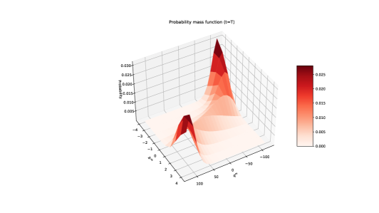
Figure 1: Joint distribution of $\displaystyle b^{m}$ and $\displaystyle q^{m}$.

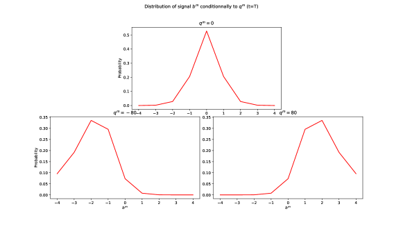
(a) Distribution of $\displaystyle b^{m}$ for a fixed $\displaystyle q^{m}$.

(b) Distribution of $\displaystyle q^{m}$ for a fixed $\displaystyle b^{m}$.

Figure 2: Conditional distributions of $\displaystyle b^{m}$ and $\displaystyle q^{m}$.

5.2 Market-takers’ behaviour: value function and optimal quotes

The value function $\displaystyle W^{m}$ is plotted at time $\displaystyle t=0$ in Figure 3. We then plot in Figure 4(a) the same value function at fixed values of $\displaystyle q^{m}$, and observe some interesting behaviours. Indeed, when $\displaystyle q^{m}=0$, the value function is symmetric but its minimum value is in $\displaystyle b^{m}=0$, meaning that even with an empty inventory, the market-taker always prefer having a positive or negative signal because this will allow him to make more profit over the time period $\displaystyle[0,T]$. This effect is even more striking in the cases $\displaystyle q^{m}=-80$ and $\displaystyle q^{m}=80$: even with an already very long or short inventory, the worst case for the market-taker is a flat signal. Indeed, when the market-taker is short, he prefers having a negative signal, but a positive signal is still better than a flat signal because he knows she can trade fast enough to become long before the signal changes. Finally, we plot in Figure 4(a) the value function at fixed values of $\displaystyle b^{m}$. The results are less surprising and match our intuition: when the signal is flat, the value function is symmetric and its maximum is in $\displaystyle 0$, because the market-taker does not have any interest in deviating from an empty position. When the signal is negative, the optimum of the value function is in the negative values for the inventory, and conversely.

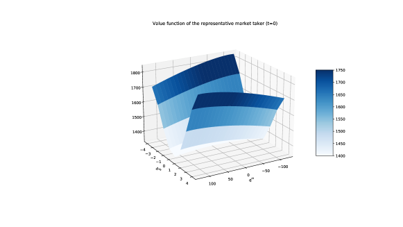
Figure 3: Value function of the representative market-taker.

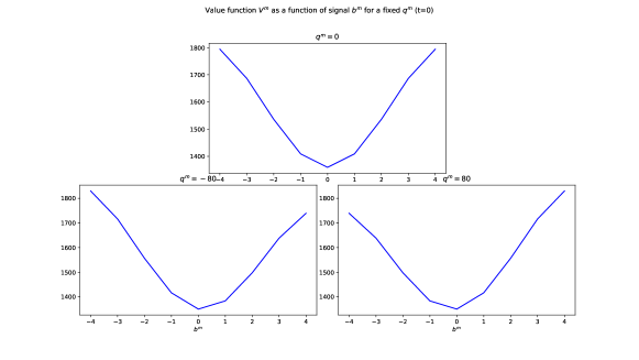
(a) For a fixed $\displaystyle q^{m}$.

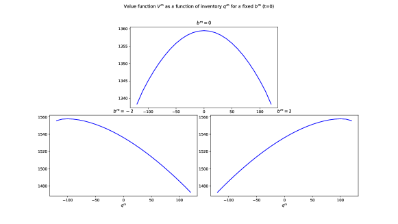
(b) For a fixed $\displaystyle b^{m}$.

Figure 4: Value function of the representative market-taker.

We plot the (stationary) optimal bid and ask quotes of the market-taker as a function of $\displaystyle q^{m}$ and $\displaystyle b^{m}$ in Figure 5. In Figure 6(a), we plot his bid quotes as a function of $\displaystyle b^{m}$ for different values of $\displaystyle q^{m}.$ We observe that when his signal is positive enough, if his inventory is non-positive, he agrees to buy the asset at a price higher than the mid price. In particular when $\displaystyle q^{m}=-80$, this is true as soon as $\displaystyle b^{m}$ is positive. Finally in Figure 6(b), we plot the optimal bid quotes as a function $\displaystyle q^{m}$ for different values of $\displaystyle b^{m}$. Again, the result is expected: when the signal is negative, the bid quotes is always high in comparison to the other cases. Conversely, for a positive signal, if his inventory is negative, the market-maker quotes a negative mid-to-bid, meaning that he agrees to buy at a price higher than the mid price.

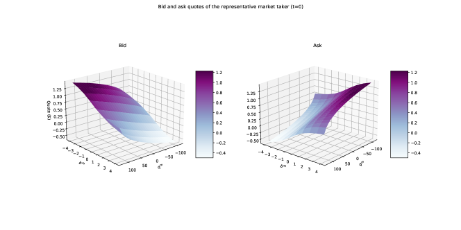
Figure 5: Optimal bid and ask quotes of the representative market-taker.

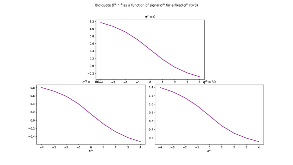
(a) For a fixed $\displaystyle q^{m}$.

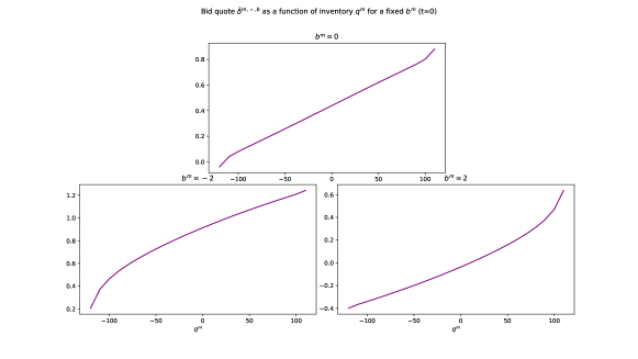
(b) For a fixed $\displaystyle b^{m}$.

Figure 6: Optimal bid quote of the representative market-taker.

5.3 Market-maker’s behaviour: value function and optimal quotes

We plot in Figure 7 the value function of the market-maker as a function of her inventory. As expected, as the market-maker is not reacting to any signal, but only make profit by providing liquidity while managing her inventory risk, the value function is symmetric with a maximum at 0. The optimal bid and ask quotes as functions of her inventory are plotted in Figure 8, with the expected behaviour: the bid quote increases with the inventory, while the ask quote decreases. The quotes of the market-maker go higher than that of the market-taker because she is more risk-averse.

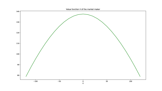
Figure 7: Value function of the market-maker.

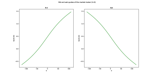
Figure 8: Optimal bid and ask quotes of the market-maker.

5.4 Impact of a more volatile signal

We now multiply by 10 the intensities $\displaystyle\lambda^{+}$and $\displaystyle\lambda^{-}$, in order to study what happens when the trading rate of the market-taker is low compared to the rate at which the signal changes.

As before, we plot in Figure 9, Figure 10(a), and Figure 10(b) the probability mass function $\displaystyle p$. We notice in particular the difference between Figure 2(b) and Figure 10(b): while the distribution of inventories is still symmetric around $\displaystyle 0$ when the signal is 0, it is now made of two ‘bumps’. This is because traders cannot react fast enough to a change of signal, so they cannot always get back to an empty inventory at the same speed as the signal goes to 0. This is also shown in Figure 10(a) in comparison with Figure 2(a): the probability that the signal is at zero when the inventory is empty is roughly 0.3 in the former case and 0.5 in the latter.

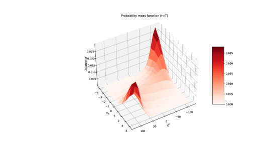
Figure 9: Joint distribution of $\displaystyle b^{m}$ and $\displaystyle q^{m}$.

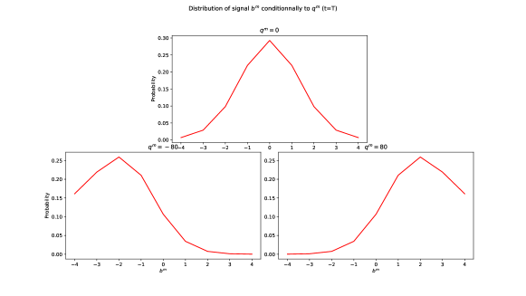
(a) Distribution of $\displaystyle b^{m}$ for a fixed $\displaystyle q^{m}$.

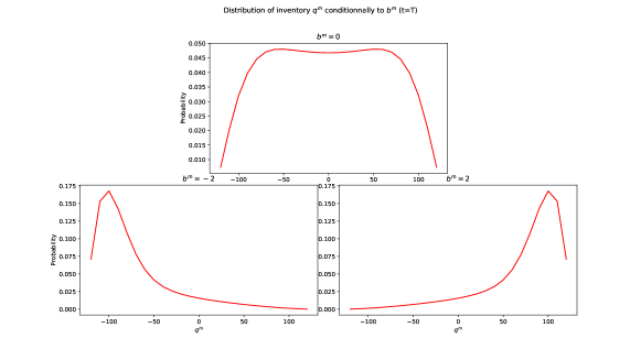
(b) Distribution of $\displaystyle q^{m}$ for a fixed $\displaystyle b^{m}$.

Figure 10: Conditional distributions of $\displaystyle b^{m}$ and $\displaystyle q^{m}$.

We now plot as above in Figure 11, Figure 12(a), and Figure 12(b) the value function $\displaystyle W^{m}$ of the market-taker at time $\displaystyle 0$ as a function of $\displaystyle q^{m}$ and $\displaystyle b^{m}$. Whereas Figure 11 and Figure 12(b) do not change much in aspect in comparison to Figure 3 and Figure 4(b), except that Figure 11 shows less difference between its highest and lowest level, due to the rapid change of the signal. Figure 12(a) is rather interesting because, unlike in Figure 4(a) the minimum of the value function when $\displaystyle q^{m}=-80$ (resp. $\displaystyle q^{m}=80$) is now reached at $\displaystyle 1$ (resp. $\displaystyle-1$) instead of $\displaystyle 0$. Unlike in the previous case, it is now less certain that the market-taker will be able to benefit from a slightly positive signal when he is short, because he cannot trade fast enough.

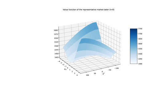
Figure 11: Value function of the representative market-taker.

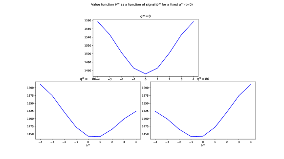
(a) For a fixed $\displaystyle q^{m}$.

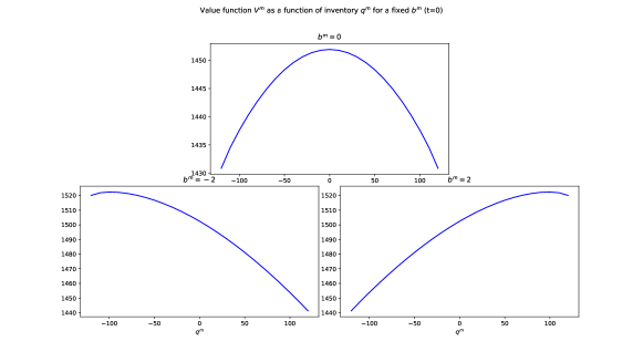
(b) For a fixed $\displaystyle b^{m}$.

Figure 12: Value function of the representative market-taker.

We then plot in Figure 13, Figure 14(a), and Figure 14(b) the optimal quotes of the representative market-taker, which are roughly at the same level as before, except for intermediate values at which the market-taker quotes more conservatively.

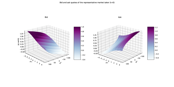
Figure 13: Optimal bid and ask quotes of the representative market-taker.

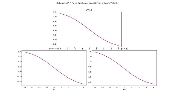
(a) For a fixed $\displaystyle q^{m}$.

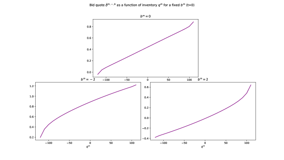
(b) For a fixed $\displaystyle b^{m}$.

Figure 14: Optimal bid quote of the representative market-taker.

We finally plot in Figure 15 the value function at time $\displaystyle 0$ of the market-maker, and in Figure 16 her optimal bid and ask quotes. While the general shape of the value function and the optimal quotes do not change much when compared to Figure 7 and Figure 8, we see that the level of the value function is significantly lower. This is due to the fact that the market-maker trades less, because market-takers are more conservatives due to the uncertainty on the signal.

Figure 15: Value function of the market-maker.

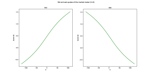
Figure 16: Optimal bid and ask quotes of the market-maker.

6 Conclusion

In this article, we tackled the problem of a market-maker on a single underlying asset facing strategical market-takers. The market-maker choses her quotes based on the behaviour of the mean-field of market-takers whose strategy is determined through an exogenous trading signal. We derive the system of HJB–Fokker–Planck equations driving this optimization problem and show existence of a solution through a fixed point argument. As the HJB equations of the market-maker and the mean-field of market-takers are decoupled, numerical resolution is simplified.

We illustrate the results of our model using a set of realistic market parameters and draw some conclusions. As expected, the probability distribution of the market-takers’ inventory shifts with the exogenous trading signal and the strategy of the market-makers are adjusted with respect to this flow of probability. Finally, a more volatile exogenous signal leads to a change in inventory distribution for the market-takers: as they cannot react fast enough to a change of signal, they are not able to get back to an empty inventory at the same speed when the signal goes to zero.

This framework can be enhanced by introducing more complex trading signals and deeper interactions between market-maker and market-takers, at the cost of an increasing numerical complexity. In particular, one could add a common noise into the signals dynamics, and make the intensity function $\displaystyle\Lambda^{m}$ of the market-takers dependent on the behaviour of the market-maker, but the problem then becomes numerically intractable, and theoretically much more complex to study.

Appendix A Proof of Theorem 4.3

We divide this proof in 4 steps. First we introduce suitable functional spaces to study these equations. Then we prove in the second step that, given a family $\displaystyle(\Pi_{t})_{t\in[0,T]}$ of probability measures on $\displaystyle\mathcal{Q}^{m}\times\mathcal{B}$, there exists a unique solution to the first two equations in (4.6). Conversely, in step 3, we prove that given two functions $\displaystyle W:[0,T]\times\mathcal{Q}\longrightarrow\mathbb{R}$ and $\displaystyle W^{m}:[0,T]\times\mathcal{Q}^{m}\times\mathcal{B}\longrightarrow\mathbb{R}$, there exists a unique solution to the last equation in (4.6). Finally, we use a fixed-point theorem to conclude.

Step 1: Functional spaces

Let us introduce the set $\displaystyle B(\mathcal{Q}^{m}\times\mathcal{B})$ of functions $\displaystyle v:\mathcal{Q}^{m}\times\mathcal{B}\longrightarrow\mathbb{R}$ that are bounded on $\displaystyle\mathcal{Q}^{m}\times\mathcal{B}$. We consider the norm $\displaystyle\|\cdot\|_{\infty}$ on $\displaystyle B(\mathcal{Q}^{m}\times\mathcal{B})$ such that for all $\displaystyle v\in B(\mathcal{Q}^{m}\times\mathcal{B}),$

$$\|v\|_{\infty}=\underset{(q^{m},b^{m})\in\mathcal{Q}^{m}\times\mathcal{B}}{\sup}|v(q^{m},b^{m})|.$$

Then $\displaystyle(B(\mathcal{Q}^{m}\times\mathcal{B}),\|\cdot\|_{\infty})$ is a Banach space. We define similarly $\displaystyle B(\mathcal{Q})$. We will also denote by $\displaystyle\bar{B}(0,1)$ the closed ball of center $\displaystyle 0$ and radius $\displaystyle 1$ in $\displaystyle B(\mathcal{Q}^{m}\times\mathcal{B})$. Note that, as $\displaystyle\mathcal{Q}^{m}\times\mathcal{B}$ is a finite set, $\displaystyle B(\mathcal{Q}^{m}\times\mathcal{B})$ has finite dimension and $\displaystyle\bar{B}(0,1)$ is compact.

Step 2: HJB equations

If we consider a continuous function $\displaystyle\tilde{p}:t\in[0,T]\longmapsto\tilde{p}_{t}\in\bar{B}(0,1)$ such that $\displaystyle\tilde{p}_{t}$ is a probability mass function on $\displaystyle\mathcal{Q}^{m}\times\mathcal{B}$, and if we denote by $\displaystyle\tilde{\Pi}$ the probability flow associated with $\displaystyle\tilde{p}$, we can then define $\displaystyle{\cal W}=\big{(}\tilde{W},\tilde{W}^{m}\big{)}$ solution to the differential equation

$$\displaystyle\partial_{t}{\cal W}(t)=F\big{(}\tilde{p}_{t},\tilde{W}(t)\big{)},\;{\cal W}(T)(q,q^{m},b^{m})=(0,0)\;\quad\forall(q,q^{m},b^{m})\in\mathcal{Q}\times\mathcal{Q}^{m}\times\mathcal{B},$$ (A.1)

where the unknown is a function $\displaystyle{\cal W}:[0,T]\longrightarrow B(\mathcal{Q})\times B(\mathcal{Q}^{m}\times\mathcal{B})$, and we denote for all $\displaystyle(q,q^{m},b^{m})\in\mathcal{Q}\times\mathcal{Q}^{m}\times\mathcal{B}$:

$${\cal W}(t)(q,q^{m},b^{m})=\big{(}\tilde{W}(t)(q),\tilde{W}^{m}(t)(q^{m},b^{m})\big{)}.$$

The function $\displaystyle F:(p,{\cal W})\in\bar{B}(0,1)\times B(\mathcal{Q})\times B(\mathcal{Q}^{m}\times\mathcal{B})\longmapsto F(p,{\cal W})\in B(\mathcal{Q})\times B(\mathcal{Q}^{m}\times\mathcal{B})$ is defined by the first two equations in Equation 4.6, i.e.

$$\displaystyle F\big{(}p,(W,W^{m})\big{)}(q,q^{m},b^{m})$$

$$\displaystyle=\bigg{(}\phi\sigma^{2}q^{2}-q\kappa\int_{\mathbb{R}^{2}}{\cal L}\Big{(}y,\bar{d}^{m}\big{(}W^{m}(t,z,y)-W^{m}(t,z,y+1)\big{)},\bar{d}^{m}\big{(}W^{m}(t,z,y)-W^{m}(t,z,y-1)\big{)}\Big{)}p(t,y,z)\mathrm{d}y\mathrm{d}z$$

$$\displaystyle\quad-\mathcal{H}\Big{(}t,q,\bar{d}\big{(}W(t,q)-W(t,q+1)\big{)},\bar{d}\big{(}W(t,q),W(t,q-1)\big{)},W(t,q),W(t,q+1),W(t,q-1),\bar{\delta}^{m},p(t,\cdot,\cdot)\Big{)},$$

$$\displaystyle\quad+\gamma\sigma^{2}(q^{m})^{2}+b^{m}q^{m}+{\cal K}\Big{(}b^{m},W^{m}(t,q^{m},b^{m}),W^{m}(t,q^{m},b^{m}+1),W^{m}(t,q^{m},b^{m}-1)\Big{)}$$

$$\displaystyle\quad-q^{m}\kappa\int_{\mathbb{R}^{2}}{\cal L}\Big{(}y,\bar{d}^{m}\big{(}W^{m}(t,z,y)-W^{m}(t,z,y+1)\big{)},\bar{d}^{m}\big{(}W^{m}(t,z,y)-W^{m}(t,z,y-1)\big{)}\Big{)}p(t,y,z)\mathrm{d}y\mathrm{d}z$$

$$\displaystyle\quad-\mathcal{H}^{m}\Big{(}q^{m},\bar{d}^{m}\big{(}W^{m}(t,q^{m},b^{m})-W^{m}(t,q^{m}+1,b^{m})\big{)},\bar{d}^{m}\big{(}W^{m}(t,q^{m},b^{m}),W^{m}(t,q^{m}-1,b^{m})\big{)},$$

$$\displaystyle\qquad\qquad W^{m}(t,q^{m},b^{m}),W^{m}(t,q^{m}+1,b^{m}),W^{m}(t,q^{m}-1,b^{m})\Big{)}\bigg{)},$$

is continuous in $\displaystyle(p,W)$, and is Lipschitz-continuous in $\displaystyle W$ because the controls are bounded (this is proved in details in Bergault and Guéant [10, Proposition 2]). Hence we know by Cauchy–Lipschitz’s theorem that for any continuous $\displaystyle\tilde{p}:t\in[0,T]\longmapsto\tilde{p}_{t}\in\bar{B}(0,1)$, there exists a unique global solution $\displaystyle\tilde{W}:[0,T]\longrightarrow B(\mathcal{Q})\times B(\mathcal{Q}^{m}\times\mathcal{B})$ to (A.1).

Step 3: Fokker–Planck equation

For a given pair of functions $\displaystyle{\cal W}=(\tilde{W},\tilde{W}^{m})$, we can write the Fokker–Planck equation in (4.6) as

$$\begin{cases}\partial_{t}p(t,\cdot,\cdot)=G(\tilde{W}^{m}(t),p(t,\cdot,\cdot)),\\ p(0,\cdot,\cdot)=P_{0},\end{cases}$$ (A.2)

where the unknown is a function $\displaystyle p:[0,T]\longrightarrow B(\mathcal{Q}^{m}\times\mathcal{B}).$ The function

$$G:(W^{m},p)\in B(\mathcal{Q}^{m}\times\mathcal{B})\times B(\mathcal{Q}^{m}\times\mathcal{B})\longmapsto G(W,p)\in B(\mathcal{Q}^{m}\times\mathcal{B}),$$

defined by the last equation in (4.6), i.e.

$$\displaystyle G\big{(}W^{m},p\big{)}(q^{m},b^{m}) \displaystyle=\mathds{1}_{\{q^{m}>-\tilde{q}^{m}\}}\Lambda^{m}\Big{(}\bar{d}^{m}\big{(}W^{m}(t,q^{m}-1,b^{m})-W^{m}(t,q^{m},b^{m})\big{)}\Big{)}p(t,q^{m}-1,b^{m})$$

$$\displaystyle\quad+\mathds{1}_{\{q^{m}<\tilde{q}^{m}\}}\Lambda^{m}\Big{(}\bar{d}^{m}\big{(}W^{m}_{(}t,q^{m}+1,b^{m})-W^{m}(t,q^{m},b^{m})\big{)}\Big{)}p(t,q^{m}+1,b^{m})$$

$$\displaystyle\quad+\bar{\lambda}^{+}\mathds{1}_{\{b^{m}>-\tilde{b}\}}p(t,q^{m},b^{m}-1)-\bar{\lambda}^{-}\mathds{1}_{\{b^{m}<\tilde{b}\}}p(t,q^{m},b^{m}+1)$$

$$\displaystyle\quad-p(t,q^{m},b^{m})\bigg{(}\mathds{1}_{\{q^{m}<\tilde{q}^{m}\}}\Lambda^{m}\Big{(}\bar{d}^{m}\big{(}W^{m}(t,q^{m},b^{m})-W^{m}(t,q^{m}+1,b^{m})\big{)}\Big{)}$$

$$\displaystyle\quad+\mathds{1}_{\{q^{m}>-\tilde{q}^{m}\}}\Lambda^{m}\Big{(}\bar{d}^{m}\big{(}W^{m}(t,q^{m},b^{m})-W^{m}(t,q^{m}-1,b^{m})\big{)}\Big{)}+\bar{\lambda}^{-}\mathds{1}_{\{b^{m}>-\tilde{b}\}}+\bar{\lambda}^{+}\mathds{1}_{\{b^{m}<\tilde{b}\}}\bigg{)},$$

is continuous in $\displaystyle(W^{m},p)$ and Lipschitz-continuous (even linear) in $\displaystyle p.$ Hence we know again from Cauchy–Lipschitz’s theorem that for any continuous $\displaystyle\tilde{W}^{m}:t\in[0,T]\longrightarrow\tilde{W}^{m}(t)\in B(\mathcal{Q}^{m}\times\mathcal{B})$, there exists a unique global solution $\displaystyle p:[0,T]\longrightarrow B(\mathcal{Q}^{m}\times\mathcal{B})$ to Equation A.2. Moreover, as (A.2) is actually a Fokker–Planck equation, we know that the solution $\displaystyle p$ verifies $\displaystyle p(t,\cdot,\cdot)\in\bar{B}(0,1)\ \forall t\in[0,T].$

Step 4: fixed-point theorem

Finally, let us define $\displaystyle X$ the set of time-dependent probability measures $\displaystyle\tilde{p}\in\mathcal{C}^{0}([0,T],\bar{B}(0,1))$ such that

$$\|\tilde{p}(t,\cdot,\cdot)-\tilde{p}(s,\cdot,\cdot)\|_{\infty}\leq L|t-s|,\;\forall\ s,t\in[0,T],$$ (A.3)

where $\displaystyle L=4\big{(}\Lambda^{m}(-\delta_{\infty})+\bar{\lambda}\big{)}.$ Note that, by Arzelà–Ascoli theorem, it is clear that $\displaystyle X$ is relatively compact for the uniform distance. If we take $\displaystyle\tilde{p}\in X$, we can associate to it the function $\displaystyle\tilde{W}$ solution to (A.1), and from the associated control we can get a new probability mass function $\displaystyle p$ solution to (A.2). Moreover, by definition of $\displaystyle L$ and of the function $\displaystyle G$ in (A.2), it is clear that $\displaystyle p$ satisfies (A.3), hence $\displaystyle p\in X$. This defines a map $\displaystyle\phi:\tilde{p}\in X\longrightarrow p=\phi(\tilde{p})\in X.$

Let us now consider $\displaystyle(\tilde{p}^{\ell})_{\ell\in\mathbb{N}}$ a sequence in $\displaystyle X$ converging uniformly to $\displaystyle\tilde{p}\in X.$ For each $\displaystyle\ell\in\mathbb{N}$, let $\displaystyle{\cal W}^{\ell}$ and $\displaystyle p^{\ell}$ be the corresponding solutions to (A.1) and (A.2), respectively. By continuity of $\displaystyle F$ and $\displaystyle G$, $\displaystyle({\cal W}^{\ell})_{\ell\in\mathbb{N}}$ will converge to the unique solution $\displaystyle{\cal W}$ to the HJB equation (A.1) associated with $\displaystyle\tilde{p},$ and in the same way $\displaystyle(p^{\ell})_{\ell\in\mathbb{N}}$ converges to the unique solution $\displaystyle p$ to the Fokker–Planck equation (A.2) associated with $\displaystyle{\cal W}$. This shows the continuity of $\displaystyle\phi$.

By Schauder’s fixed-point theorem, we conclude that $\displaystyle\phi$ has a fixed-point $\displaystyle p$, and by denoting $\displaystyle{\cal W}=(W,W^{m})$ the associated solution to (A.1), we get that $\displaystyle(W,W^{m},p)$ is solution to the master equation (4.6).

Appendix B Proof of Theorem 4.4

We fix $\displaystyle t\in[0,T)$.

Step 1: First, let us look at the problem of the market-maker. We introduce the arbitrary controls $\displaystyle(\delta^{b}_{s})_{s\in[t,T]}$ and $\displaystyle(\delta^{a}_{s})_{s\in[t,T]}$ for the market-maker, and denote by $\displaystyle(q_{s})_{s\in[t,T]}$ her inventory process starting at time $\displaystyle t$, respectively at the value $\displaystyle q\in\mathcal{Q}$, and controlled by $\displaystyle(\delta^{b}_{s})_{s\in[t,T]}$ and $\displaystyle(\delta^{a}_{s})_{s\in[t,T]}$. Then, under $\displaystyle\mathbb{P}^{\delta,\bar{\delta}^{m,\star},\mathcal{V}(\bar{\delta}^{m,\star},\tilde{\Pi})}$, we have

$$\displaystyle\tilde{W}(T,q_{T}) \displaystyle=\tilde{W}(t,q)+\int_{t}^{T}\partial_{t}\tilde{W}(s,q_{s})\mathrm{d}s+\int_{t}^{T}\big{(}\tilde{W}(s,q_{s-}+1)-\tilde{W}(s,q_{s-})\big{)}\mathrm{d}N^{b}_{s}+\int_{t}^{T}\big{(}\tilde{W}(s,q_{s-}-1)-\tilde{W}(s,q_{s-})\big{)}\mathrm{d}N^{a}_{s}$$

$$\displaystyle=\tilde{W}(t,q)+\int_{t}^{T}\partial_{t}\tilde{W}(s,q_{s})\mathrm{d}s$$

$$\displaystyle\quad+\int_{t}^{T}\big{(}\tilde{W}(s,q_{s-}+1)-\tilde{W}(s,q_{s-})\big{)}\mathds{1}_{\{q_{s-}<\tilde{q}\}}\Lambda\bigg{(}\int_{\mathbb{R}^{2}}\delta^{m,\star,a}(s,z,y,\tilde{\Pi}_{s})\tilde{\Pi}_{s}(\mathrm{d}y,\mathrm{d}z),\delta^{b}_{s}\bigg{)}\mathrm{d}s$$

$$\displaystyle\quad+\int_{t}^{T}\big{(}\tilde{W}(s,q_{s-}-1)-\tilde{W}(s,q_{s-})\big{)}\mathds{1}_{\{q_{s-}>-\tilde{q}\}}\Lambda\bigg{(}\int_{\mathbb{R}^{2}}\delta^{m,\star,b}(s,z,y,\tilde{\Pi}_{s})\tilde{\Pi}_{s}(\mathrm{d}y,\mathrm{d}z),\delta^{a}_{s}\bigg{)}\mathrm{d}s$$

$$\displaystyle\quad+\int_{t}^{T}\big{(}\tilde{W}(s,q_{s-}+1)-\tilde{W}(s,q_{s-})\big{)}\mathrm{d}\tilde{N}^{b}_{s}+\int_{t}^{T}\big{(}\tilde{W}(s,q_{s-}-1)-\tilde{W}(s,q_{s-})\big{)}\mathrm{d}\tilde{N}^{a}_{s},$$

where $\displaystyle\tilde{N}^{b}$ and $\displaystyle\tilde{N}^{a}$ are the compensated processes associated to $\displaystyle N^{b}$ and $\displaystyle N^{a}$ under $\displaystyle\mathbb{P}^{\delta,\bar{\delta}^{m,\star},\mathcal{V}(\bar{\delta}^{m,\star},\tilde{\Pi})}$. We can then write

$$\displaystyle\tilde{W}(T,q_{T}) \displaystyle=\tilde{W}(t,q)+\int_{t}^{T}\Bigg{(}\partial_{t}\tilde{W}(s,q_{s})-\phi\sigma^{2}(q_{s})^{2}$$

$$\displaystyle\quad+\Big{(}\delta^{b}_{s}+\tilde{W}(s,q_{s-}+1)-\tilde{W}(s,q_{s-})\Big{)}\mathds{1}_{\{q_{s-}<\tilde{q}\}}\Lambda\bigg{(}\int_{\mathbb{R}^{2}}\delta^{m,\star,a}(s,z,y,\tilde{\Pi}_{s})\tilde{\Pi}_{s}(\mathrm{d}y,\mathrm{d}z),\delta^{b}_{s}\bigg{)}$$

$$\displaystyle\quad+\Big{(}\delta^{a}_{s}+\tilde{W}(s,q_{s-}-1)-\tilde{W}(s,q_{s-})\Big{)}\mathds{1}_{\{q_{s-}>-\tilde{q}\}}\Lambda\bigg{(}\int_{\mathbb{R}^{2}}\delta^{m,\star,b}(s,z,y,\tilde{\Pi}_{s})\tilde{\Pi}_{s}(\mathrm{d}y,\mathrm{d}z),\delta^{a}_{s}\bigg{)}$$

$$\displaystyle\quad+q_{s}\kappa\int_{\mathbb{R}^{2}}{\cal L}\Big{(}y,\bar{d}^{m}\big{(}\tilde{W}^{m}(t,z,y)-\tilde{W}^{m}(t,z,y+1)\big{)},\bar{d}^{m}\big{(}\tilde{W}^{m}(t,z,y)-\tilde{W}^{m}(t,z,y-1)\big{)}\Big{)}\Pi_{t}(\mathrm{d}y,\mathrm{d}z)\Bigg{)}\mathrm{d}s$$

$$\displaystyle\quad+\int_{t}^{T}\Bigg{(}\phi\sigma^{2}(q_{s})^{2}-\delta^{b}_{s}\mathds{1}_{\{q_{s-}<\tilde{q}\}}\Lambda\bigg{(}\int_{\mathbb{R}^{2}}\delta^{m,\star,a}(s,z,y,\tilde{\Pi}_{s})\tilde{\Pi}_{s}(\mathrm{d}y,\mathrm{d}z),\delta^{b}_{s}\bigg{)}$$

$$\displaystyle\quad-\delta^{a}_{s}\mathds{1}_{\{q_{s-}>-\tilde{q}\}}\Lambda\bigg{(}\int_{\mathbb{R}^{2}}\delta^{m,\star,b}(s,z,y,\tilde{\Pi}_{s})\tilde{\Pi}_{s}(\mathrm{d}y,\mathrm{d}z),\delta^{a}_{s}\bigg{)}$$

$$\displaystyle\quad-q_{s}\kappa\int_{\mathbb{R}^{2}}{\cal L}\Big{(}y,\bar{d}^{m}\big{(}\tilde{W}^{m}(t,z,y)-\tilde{W}^{m}(t,z,y+1)\big{)},\bar{d}^{m}\big{(}\tilde{W}^{m}(t,z,y)-\tilde{W}^{m}(t,z,y-1)\big{)}\Big{)}\Pi_{t}(\mathrm{d}y,\mathrm{d}z)\Bigg{)}\mathrm{d}s$$

$$\displaystyle\quad+\int_{t}^{T}\big{(}\tilde{W}(s,q_{s-}+1)-\tilde{W}(s,q_{s-})\big{)}\mathrm{d}\tilde{N}^{b}_{s}+\int_{t}^{T}\big{(}\tilde{W}(s,q_{s-}-1)-\tilde{W}(s,q_{s-})\big{)}\mathrm{d}\tilde{N}^{a}_{s}.$$

From the HJB equation solved by $\displaystyle\tilde{W}$ and the associated terminal condition $\displaystyle\tilde{W}(T,.)=0$, we deduce

$$\displaystyle 0 \displaystyle\leq\tilde{W}(t,q)+\int_{t}^{T}\bigg{(}\phi\sigma^{2}(q_{s})^{2}-\delta^{b}_{s}\mathds{1}_{\{q_{s-}<\tilde{q}\}}\Lambda\bigg{(}\int_{\mathbb{R}^{2}}\delta^{m,\star,a}(s,z,y,\tilde{\Pi}_{s})\tilde{\Pi}_{s}(\mathrm{d}y,\mathrm{d}z),\delta^{b}_{s}\bigg{)}$$

$$\displaystyle\quad-\delta^{a}_{s}\mathds{1}_{\{q_{s-}>-\tilde{q}\}}\Lambda\bigg{(}\int_{\mathbb{R}^{2}}\delta^{m,\star,b}(s,z,y,\tilde{\Pi}_{s})\tilde{\Pi}_{s}(\mathrm{d}y,\mathrm{d}z),\delta^{a}_{s}\bigg{)}$$

$$\displaystyle\quad-q_{s}\kappa\int_{\mathbb{R}^{2}}{\cal L}\Big{(}y,\bar{d}^{m}\big{(}\tilde{W}^{m}(t,z,y)-\tilde{W}^{m}(t,z,y+1)\big{)},\bar{d}^{m}\big{(}\tilde{W}^{m}(t,z,y)-\tilde{W}^{m}(t,z,y-1)\big{)}\Big{)}\Pi_{t}(\mathrm{d}y,\mathrm{d}z)\bigg{)}\mathrm{d}s$$

$$\displaystyle\quad+\int_{t}^{T}\big{(}\tilde{W}(s,q_{s-}+1)-\tilde{W}(s,q_{s-})\big{)}\mathrm{d}\tilde{N}^{b}_{s}+\int_{t}^{T}\big{(}\tilde{W}(s,q_{s-}-1)-\tilde{W}(s,q_{s-})\big{)}\mathrm{d}\tilde{N}^{a}_{s}.$$

Notice that $\displaystyle\tilde{N}^{b}$ and $\displaystyle\tilde{N}^{a}$ are martingales under $\displaystyle\mathbb{P}^{\delta,\bar{\delta}^{m,\star},\mathcal{V}(\bar{\delta}^{m,\star},\tilde{\Pi})}$, since by definition of $\displaystyle\mathcal{A}_{\infty}$, their intensities are bounded. Taking expectation yields

$$\displaystyle\begin{split}\tilde{W}(t,q)&\geq\mathbb{E}^{\delta,\bar{\delta}^{m,\star},\mathcal{V}(\bar{\delta}^{m,\star},\tilde{\Pi})}\Bigg{[}\int_{t}^{T}\bigg{(}-\phi\sigma^{2}(q_{s})^{2}+\delta^{b}_{s}\mathds{1}_{\{q_{s-}<\tilde{q}\}}\Lambda\bigg{(}\int_{\mathbb{R}^{2}}\delta^{m,\star,a}(s,z,y,\tilde{\Pi}_{s})\tilde{\Pi}_{s}(\mathrm{d}y,\mathrm{d}z),\delta^{b}_{s}\bigg{)}\\ &\quad+\delta^{a}_{s}\mathds{1}_{\{q_{s-}>-\tilde{q}\}}\Lambda\bigg{(}\int_{\mathbb{R}^{2}}\delta^{m,\star,b}(s,z,y,\tilde{\Pi}_{s})\tilde{\Pi}_{s}(\mathrm{d}y,\mathrm{d}z),\delta^{a}_{s}\bigg{)}\\ &\quad+q_{s}\kappa\int_{\mathbb{R}^{2}}{\cal L}\Big{(}y,\bar{d}^{m}\big{(}\tilde{W}^{m}(t,z,y)-\tilde{W}^{m}(t,z,y+1)\big{)},\bar{d}^{m}\big{(}\tilde{W}^{m}(t,z,y)-\tilde{W}^{m}(t,z,y-1)\big{)}\Big{)}\Pi_{t}(\mathrm{d}y,\mathrm{d}z)\bigg{)}\mathrm{d}s\Bigg{]},\end{split}$$ (B.1)

with equality when the market-maker plays the controls in (4.8).

By taking the supremum in (B.1), we get that $\displaystyle\tilde{W}(0,q_{0})=\tilde{V}(\bar{\delta}^{m},\tilde{\Pi})$, and the controls given in (4.8) are optimal for the market-maker when the market-taker plays the controls given again in (4.8).

Step 2: We show by the same argument that $\displaystyle\tilde{W}^{m}(0,q^{m}_{0},b^{m}_{0})=\tilde{V}^{m}(\bar{\delta}^{m},\tilde{\Pi})$ and that the controls given in (4.8) are optimal for the market-taker when the market-maker plays his respective controls in (4.8).

References

- Almgren and Chriss [2001] R.F. Almgren and N. Chriss. Optimal execution of portfolio transactions. Journal of Risk, 3(2):5–40, 2001.
- Avellaneda and Stoikov [2008] M. Avellaneda and S. Stoikov. High-frequency trading in a limit order book. Quantitative Finance, 8(3):217–224, 2008.
- Baldacci and Manziuk [2020] B. Baldacci and I. Manziuk. Adaptive trading strategies across liquidity pools. ArXiv preprint arXiv:2008.07807, 2020.
- Baldacci et al. [2020] B. Baldacci, P. Bergault, J. Derchu, and M. Rosenbaum. On bid and ask side–specific tick sizes. ArXiv preprint arXiv:2005.14126, 2020.
- Baldacci et al. [2021a] B. Baldacci, P. Bergault, and O. Guéant. Algorithmic market making for options. Quantitative Finance, 21(1):85–97, 2021a.
- Baldacci et al. [2021b] B. Baldacci, D. Possamaï, and M. Rosenbaum. Optimal make take fees in a multi market maker environment. SIAM Journal on Financial Mathematics, 12(1):446–486, 2021b.
- Barzykin et al. [2021a] A. Barzykin, P. Bergault, and O. Guéant. Algorithmic market making in foreign exchange cash markets with hedging and market impact. ArXiv preprint arXiv:2106.06974, 2021a.
- Barzykin et al. [2021b] A. Barzykin, P. Bergault, and O. Guéant. Market making by an FX dealer: tiers, pricing ladders and hedging rates for optimal risk control. ArXiv preprint arXiv:2112.02269, 2021b.
- Bayraktar and Chakraborty [2021] E. Bayraktar and P. Chakraborty. Mean field control and finite dimensional approximation for regime-switching jump diffusions. arXiv preprint arXiv:2109.09134, 2021.
- Bergault and Guéant [2021] P. Bergault and O. Guéant. Size matters for OTC market makers: general results and dimensionality reduction techniques. Mathematical Finance, 31(1):279–322, 2021.
- Bergault et al. [2021] P. Bergault, D. Evangelista, O. Guéant, and D. Vieira. Closed-form approximations in multi-asset market making. Applied Mathematical Finance, 28(2):101–142, 2021.
- Buckdahn et al. [2014] R. Buckdahn, J. Li, and S. Peng. Nonlinear stochastic differential games involving a major player and a large number of collectively acting minor agents. SIAM Journal on Control and Optimization, 52(1):451–492, 2014.
- Cardaliaguet and Lehalle [2018] P. Cardaliaguet and C.-A. Lehalle. Mean field game of controls and an application to trade crowding. Mathematics and Financial Economics, 12(3):335–363, 2018.
- Cardaliaguet et al. [2020] P. Cardaliaguet, M. Cirant, and A. Porretta. Remarks on Nash equilibria in mean field game models with a major player. Proceedings of the American Mathematical Society, 148(10):4241–4255, 2020.
- Carmona and Wang [2016] R. Carmona and P. Wang. Finite state mean field games with major and minor players. ArXiv preprint arXiv:1610.05408, 2016.
- Carmona and Wang [2017] R. Carmona and P. Wang. An alternative approach to mean field game with major and minor players, and applications to herders impacts. Applied Mathematics & Optimization, 76(1):5–27, 2017.
- Carmona and Zhu [2016] R. Carmona and X. Zhu. A probabilistic approach to mean field games with major and minor players. The Annals of Applied Probability, 26(3):1535–1580, 2016.
- Cartea and Jaimungal [2016] Á. Cartea and S. Jaimungal. Incorporating order-flow into optimal execution. Mathematics and Financial Economics, 10(3):339–364, 2016.
- Cartea et al. [2015] Á. Cartea, S. Jaimungal, and J. Penalva. Algorithmic and high-frequency trading. Cambridge University Press, 2015.
- Cartea et al. [2017] Á. Cartea, R. Donnelly, and S. Jaimungal. Algorithmic trading with model uncertainty. SIAM Journal on Financial Mathematics, 8(1):635–671, 2017.
- Cartea et al. [2018] Á. Cartea, R. Donnelly, and S. Jaimungal. Enhancing trading strategies with order book signals. Applied Mathematical Finance, 25(1):1–35, 2018.
- Casgrain and Jaimungal [2018] P. Casgrain and S. Jaimungal. Mean field games with partial information for algorithmic trading. ArXiv preprint arXiv:1803.04094, 2018.
- Casgrain and Jaimungal [2020] P. Casgrain and S. Jaimungal. Mean-field games with differing beliefs for algorithmic trading. Mathematical Finance, 30(3):995–1034, 2020.
- Dayri and Rosenbaum [2015] K. Dayri and M. Rosenbaum. Large tick assets: implicit spread and optimal tick size. Market Microstructure and Liquidity, 1(01):1550003, 2015.
- El Euch et al. [2021] O. El Euch, T. Mastrolia, M. Rosenbaum, and N. Touzi. Optimal make-take fees for market making regulation. Mathematical Finance, to appear, 2021.
- Firoozi and Caines [2019] D. Firoozi and P.E. Caines. Belief estimation by agents in major minor LQG mean field games. In C.C. de Wit and R. Sepulchre, editors, 58th IEEE conference on decision and control, 2019, pages 1615–1622. IEEE, 2019.
- Firoozi and Caines [2021] D. Firoozi and P.E. Caines. -Nash equilibria for major–minor LQG mean field games with partial observations of all agents. IEEE Transactions on Automatic Control, 66(6):2778–2786, 2021.
- Firoozi et al. [2020] D. Firoozi, S. Jaimungal, and P.E. Caines. Convex analysis for LQG systems with applications to major–minor lqg mean-field game systems. Systems & Control Letters, 142:104734, 2020.
- Grossman and Miller [1988] S.J. Grossman and M.H. Miller. Liquidity and market structure. The Journal of Finance, 43(3):617–633, 1988.
- Guéant and Manziuk [2019] O. Guéant and I. Manziuk. Deep reinforcement learning for market making in corporate bonds: beating the curse of dimensionality. Applied Mathematical Finance, 26(5):387–452, 2019.
- Guéant et al. [2013] O. Guéant, C.-A. Lehalle, and J. Fernandez-Tapia. Dealing with the inventory risk: a solution to the market making problem. Mathematics and Financial Economics, 7(4):477–507, 2013.
- Guilbaud and Pham [2013] F. Guilbaud and H. Pham. Optimal high-frequency trading with limit and market orders. Quantitative Finance, 13(1):79–94, 2013.
- Ho and Stoll [1981] T. Ho and H.R. Stoll. Optimal dealer pricing under transactions and return uncertainty. Journal of Financial Economics, 9(1):47–73, 1981.
- Huang et al. [2016] J. Huang, S. Wang, and Z. Wu. Backward–forward linear–quadratic mean-field games with major and minor agents. Probability, Uncertainty and Quantitative Risk, 1(8):1–27, 2016.
- Huang [2010] M. Huang. Large-population LQG games involving a major player: the Nash certainty equivalence principle. SIAM Journal on Control and Optimization, 48(5):3318–3353, 2010.
- Huang [2021] M. Huang. Linear–quadratic mean field games with a major player: Nash certainty equivalence versus master equations. Communications in Information and Systems, 21(3):441–471, 2021.
- Huang and Nguyen [2019] M. Huang and S.L. Nguyen. Linear–quadratic mean field social optimization with a major player. ArXiv preprint arXiv:1904.03346, 2019.
- Huang et al. [2019] X. Huang, S. Jaimungal, and M. Nourian. Mean-field game strategies for optimal execution. Applied Mathematical Finance, 26(2):153–185, 2019.
- Lasry and Lions [2018] J.-M. Lasry and P.-L. Lions. Mean-field games with a major player. Comptes Rendus Mathématique, 356(8):886–890, 2018.
- Madhavan et al. [1997] A. Madhavan, M. Richardson, and M. Roomans. Why do security prices change? A transaction-level analysis of NYSE stocks. The Review of Financial Studies, 10(4):1035–1064, 1997.
- Manziuk [2019] I. Manziuk. Optimal control and machine learning in finance: contributions to the literature on optimal execution, market making, and exotic options. PhD thesis, Université Paris 1 Panthéon–Sorbonne, 2019.
- Megarbane et al. [2017] N. Megarbane, P. Saliba, C.-A. Lehalle, and M. Rosenbaum. The behavior of high-frequency traders under different market stress scenarios. Market Microstructure and Liquidity, 3(03n04):1850005, 2017.
- Robert and Rosenbaum [2011] C.Y. Robert and M. Rosenbaum. A new approach for the dynamics of ultra–high-frequency data: the model with uncertainty zones. Journal of Financial Econometrics, 9(2):344–366, 2011.
- Wyart et al. [2008] M. Wyart, J.-P. Bouchaud, J. Kockelkoren, M. Potters, and M. Vettorazzo. Relation between bid–ask spread, impact and volatility in order-driven markets. Quantitative Finance, 8(1):41–57, 2008.