Two-neutrino double-$\beta$ decay in the mapped interacting boson model

Abstract

A calculation of two-neutrino double-$\beta$ ($2\nu\beta\beta$) decay matrix elements within the interacting boson model (IBM) that is based on the nuclear density functional theory is presented. The constrained self-consistent mean-field (SCMF) calculation using a universal energy density functional (EDF) and a pairing interaction provides potential energy surfaces with triaxial quadrupole degrees of freedom for even-even nuclei corresponding to the initial and final states of the $2\nu\beta\beta$ decays of interest. The SCMF energy surface is then mapped onto the bosonic one, and this procedure determines the IBM Hamiltonian for the even-even nuclei. The same SCMF calculation provides the essential ingredients of the interacting boson fermion-fermion model (IBFFM) for the intermediate odd-odd nuclei and the Gamow-Teller and Fermi transition operators. The EDF-based IBM and IBFFM provide a simultaneous description of excitation spectra and electromagnetic transition rates for each nucleus, and single-$\beta$ and $\beta\beta$ decay properties. The calculated $2\nu\beta\beta$-decay nuclear matrix elements are compared with experiment and with those from earlier theoretical calculations.

I Introduction

Double-$\beta$ ($\beta\beta$) decay is a fundamental nuclear process that is expected to occur between the atomic nuclei with $(A,Z)$ and $(A,Z\pm 2)$. The process can be classified into basically two types of the decay mode according to whether or not it emits neutrinos/antineutrinos, that is, whether or not the process conserves the number of leptons. Neutrinoless $\beta\beta$ ($0\nu\beta\beta$) decay is a lepton-number-violating nuclear process that does not emit neutrinos and is allowed to occur if neutrinos have mass and are Majorana particles, i.e., they are their own antiparticles. The $0\nu\beta\beta$ decay has a number of implications for the various symmetry properties of the standard model of the electroweak interactions and, in that context, experiments have been performed at a number of facilities around the world, that are aimed at the direct observations of the decay and determination of its half-life (see, e.g., Refs. [1, 2], and references are therein). There have also been extensive theoretical investigations on the $\beta\beta$ decay, with much emphasis on the zero-neutrino modes [3, 4, 5, 6, 7, 8, 9, 10, 11]. In particular, the reliable prediction of the $0\nu\beta\beta$-decay half-life requires inputs from nuclear-structure theory through the accurate calculation of the nuclear matrix element (NME), and numerous attempts have been made for the calculation of the $0\nu\beta\beta$-decay NME from a number of theoretical approaches at various levels of sophistication (see Ref. [11] for a recent review).

Another type of the $\beta\beta$ decay is the two-neutrino $\beta\beta$ ($2\nu\beta\beta$) decay. This decay process involves two electrons (or positrons) and two electron antineutrinos (or electron neutrinos), and occurs regardless of whether or not the neutrinos are their antiparticles. Since this nuclear process conserves lepton number, it is allowed by the standard model, and indeed has been observed in a number of experiments, a recent compilation of the $2\nu\beta\beta$-decay data being provided, e.g., in Ref. [12]. Given a wealth of the experimental data, theoretical calculation of the $2\nu\beta\beta$-decay properties serves as a meaningful benchmark for a given theoretical model. Furthermore, most of the theoretical tools that are needed for calculating the $2\nu\beta\beta$-decay NME, including the model assumptions and parameters, and the calculated wave functions for the initial and final even-even nuclei can be commonly used for the prediction of the $0\nu\beta\beta$-decay NME.

In the calculations of $0\nu\beta\beta$-decay NME, on one hand, the closure approximation has been frequently used, since the virtual neutrinos exchanged in the process have momenta much larger ($\approx 100$ MeV) than the typical energy scale of nuclear excitations ($\approx 10$ MeV). In the case of the $2\nu\beta\beta$ decay, on the other hand, the neutrino momenta are about the same order of magnitude as the nuclear excitation energies, hence the closure approximation is not expected to be very good. One would then have to explicitly calculate the intermediate states of the neighboring odd-odd nuclei, and their single-$\beta$ decay matrix elements. Calculations for the $\beta\beta$ decay without using the closure approximations have been performed, e.g., within the quasiparticle random-phase approximation (QRPA) [7, 13, 14], the large-scale shell model (LSSM) [15, 16, 17, 18, 19, 20], and the interacting boson model (IBM) [21].

This paper presents a calculation of the $2\nu\beta\beta$-decay NMEs within the framework of the IBM that is based on the nuclear density functional theory. The starting point shall be a set of the constrained self-consistent mean-field (SCMF) calculations [22] using a universal EDF and a pairing interaction [22, 23, 24, 25, 26] to yield potential energy surfaces as functions of the triaxial quadrupole deformations for the even-even nuclei involved in the $\beta\beta$ decays of ⁴⁸Ca, ⁷⁶Ge, ⁸²Se, ⁹⁶Zr, ¹⁰⁰Mo, ¹¹⁰Pd, ¹¹⁶Cd, ¹²⁴Sn, ¹²⁸Te, ¹³⁰Te, ¹³⁶Xe, ¹⁵⁰Nd, and ¹⁹⁸Pt. The SCMF energy surface is then mapped onto the corresponding bosonic one, and the strength parameters of the IBM Hamiltonian for describing spectroscopic properties of the even-even nuclei are determined by this mapping procedure [27]. Here the closure approximation is not made, but the intermediate states of the odd-odd neighbors are explicitly calculated in the interacting boson-fermion-fermion model (IBFFM) [28, 29]. The essential ingredients of the IBFFM and the Gamow-Teller and Fermi transition operators are provided by the same SCMF method [30, 31]. The resulting IBM and IBFFM wave functions are then used to compute single-$\beta$ and $2\nu\beta\beta$ decay properties.

The aforementioned SCMF-to-IBM mapping procedure [27], and its extensions to odd-mass and odd-odd nuclear systems [30, 31], have so far been applied to and shown to be valid in the studies of various nuclear structure phenomena in medium-heavy and heavy nuclei in a wide range of the nuclear chart, including the shape evolution and coexistence [32, 33, 34], the onset of octupole deformation and octupole collective excitations [35, 36], the quantum phase transitions in odd-mass nuclear systems [37, 38], and the $\beta$ decays of the odd-$A$ [39] and even-$A$ [40] nuclei in the mass $A\approx 130$ region. It is then another purpose of this paper to investigate whether the EDF-based IBM and IBFFM approaches are able to give a consistent description of the spectroscopic properties of low-lying states for each relevant nucleus and single-$\beta$ and $2\nu\beta\beta$-decay matrix elements.

At this point, it is worth noting that for the last decade the IBM framework has been extensively applied to the studies of $\beta\beta$ decays [41, 42, 43, 44, 45, 46]. In these references, wave functions of the IBM Hamiltonian that gives an excellent phenomenological description of the relevant even-even nuclei were used for computing the $\beta\beta$ decay NMEs, while the $\beta\beta$-decay operators were derived from multi-nucleon systems within the generalized seniority scheme [47]. A calculation of the $2\nu\beta\beta$ decays of ¹²⁸Te and ¹³⁰Te without the closure approximation was also made within the IBM and IBFFM with the ingredients determined mostly on phenomenological grounds [21]. In Ref. [48], an isospin invariant version of the IBM that is derived from a realistic shell-model interaction has been employed to identify the importance of neutron-proton isoscalar pairing in the $0\nu\beta\beta$ decay in the ⁴⁸Ca region.

The paper is organized as follows. In Sec. II, the theoretical procedures to construct the IBM and IBFFM Hamiltonians and the $\beta\beta$-decay operators are outlined. In Sec. III, calculated excitation spectra of the even-even initial and final nuclei, and odd-odd intermediate nuclei are briefly discussed. Section IV presents the calculated single-$\beta$-decay properties between the even-even and odd-odd nuclei. In Sec. V, results for the $2\nu\beta\beta$-decay NMEs in comparison with the experimental and earlier theoretical values, and effective values of the axial vector coupling constant are shown. In the same section the sensitivity of the results to several model assumptions is investigated. Finally, Sec. VI gives a summary of the main results.

II Theoretical framework

II.1 Self-consistent mean-field calculations

The constrained SCMF calculations for the even-even nuclei are performed within the relativistic Hartree-Bogoliubov (RHB) framework [24, 25, 49] with the density-dependent point-coupling (DD-PC1) [50] functional for the particle-hole channel, and a separable pairing force of finite range [51] for the particle-particle channel. The constraints are imposed on the mass quadrupole moments, which are related to the axially-symmetric deformation $\beta$ and triaxiality $\gamma$ [52]. The constrained calculations produce the potential energy surface as a function of the $\beta$ and $\gamma$ deformations, which is denoted as $E_{\mathrm{SCMF}}(\beta,\gamma)$.

The contour plots of the SCMF $(\beta,\gamma)$-deformation energy surfaces are shown in Fig. 1. For many of the nuclei, either a nearly spherical minimum with $\beta\approx 0$, or an axially-symmetric prolate $(\beta\neq 0,\gamma=0^{\circ})$, or oblate $(\beta\neq 0,\gamma=60^{\circ})$ minimum occurs in their energy surfaces. For the mass $A\approx 100$ nuclei, the energy surfaces are notably soft especially in $\gamma$ direction, with a shallow triaxial minimum within the range $20^{\circ}<\gamma<50^{\circ}$. The softness implies that a substantial degree of shape mixing is expected to occur near the ground state. For the rare-earth nuclei ¹⁵⁰Nd and ¹⁵⁰Sm, a well-developed axially-deformed prolate deformation is suggested, with the minimum at $(\beta,\gamma)\approx(0.3,0^{\circ})$. There are also considerable differences between the topology of the energy surfaces for initial and final states of a given $2\nu\beta\beta$ decay. For instance, the energy surface for the nucleus ⁷⁶Ge exhibits a prolate deformed minimum, while the oblate ground state is predicted for the corresponding final-state nucleus ⁷⁶Se.

In addition to the DD-PC1 EDF, the same constrained RHB calculations have been carried out for a couple of cases, based on the density-dependent meson-exchange (DD-ME2) interaction [53], another representative relativistic functional. It is shown, however, that essentially no notable qualitative or quantitative difference emerges between the SCMF results obtained with the DD-PC1 and DD-ME2 EDFs.

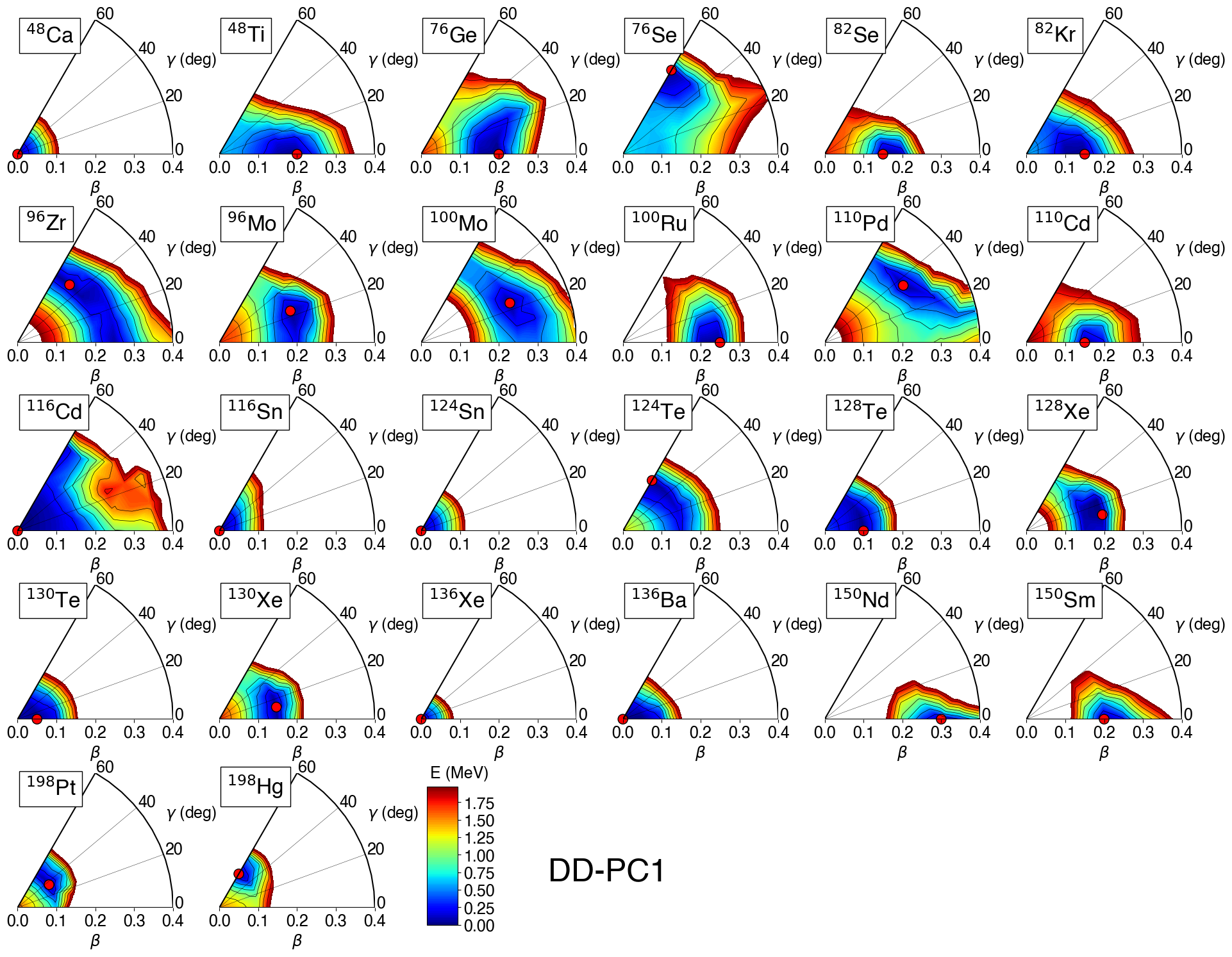
Figure 1: SCMF quadrupole triaxial $(\beta,\gamma)$ deformation energy surfaces for the initial and final even-even nuclei in the $2\nu\beta\beta$ decays under study. The energy difference between neighboring contours is 250 keV. The global minimum is identified by the solid circle.

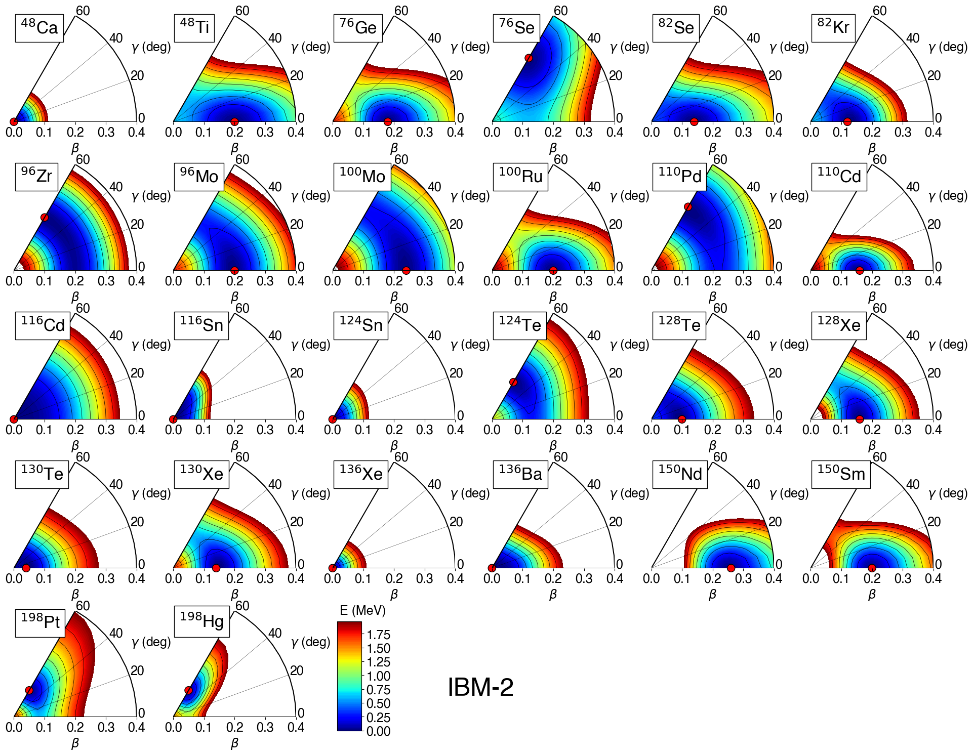
Figure 2: Same as Fig. 1, but for the IBM-2 energy surfaces.

II.2 IBM-2 for initial and final nuclei

In the present study the neutron-proton IBM (IBM-2) [47] is considered, since its connection to a microscopic picture is clearer than the original version of the model (IBM-1), which does not make a distinction between the neutron and proton degrees of freedom. The IBM-2 is built on the neutron and proton monopole ($s_{\nu}$ and $s_{\pi}$), and quadrupole ($d_{\nu}$ and $d_{\pi}$) bosons. From a microscopic point of view [54, 47], the $s_{\nu}$ ($s_{\pi}$) and $d_{\nu}$ ($d_{\pi}$) bosons are associated with the collective $S_{\nu}$ ($S_{\pi}$) and $D_{\nu}$ ($D_{\pi}$) pairs of valence neutrons (protons) with angular momenta $J=0^{+}$ and $J=2^{+}$, respectively.

The IBM-2 Hamiltonian employed in this study takes the form

$$\hat{H}_{\mathrm{B}}= \epsilon_{d}(\hat{n}_{d_{\nu}}+\hat{n}_{d_{\pi}})+\kappa\hat{Q}_{\nu}\cdot\hat{Q}_{\pi}$$

$$+\kappa_{\nu}\hat{Q}_{\nu}\cdot\hat{Q}_{\nu}+\kappa_{\pi}\hat{Q}_{\pi}\cdot\hat{Q}_{\pi}+\kappa^{\prime}\hat{L}\cdot\hat{L},$$ (1)

where in the first term, $\hat{n}_{d_{\rho}}=d^{\dagger}_{\rho}\cdot\tilde{d}_{\rho}$ ($\rho=\nu,\pi$) is the $d$-boson number operator, with $\epsilon_{d}$ the single $d$-boson energy relative to the $s$-boson one, and $\tilde{d}_{\rho\mu}=(-1)^{\mu}d_{\rho-\mu}$. The second term is the quadrupole-quadrupole interaction between neutron and proton bosons, with $\hat{Q}_{\rho}=d_{\rho}^{\dagger}s_{\rho}+s_{\rho}^{\dagger}\tilde{d}_{\rho}^{\dagger}+\chi_{\rho}(d^{\dagger}_{\rho}\times\tilde{d}_{\rho})^{(2)}$ the bosonic quadrupole operator. The third and fourth terms are the quadrupole-quadrupole interactions between identical bosons. From the microscopic considerations [54], in medium-heavy and heavy nuclei, the quadrupole-quadrupole interaction between non-identical bosons $\hat{Q}_{\nu}\cdot\hat{Q}_{\pi}$ is shown to be more important than the ones between identical bosons. In most cases, therefore, the interaction terms between identical bosons $\hat{Q}_{\rho}\cdot\hat{Q}_{\rho}$ are omitted here, but are considered only for those nuclei with $N_{\pi}=0$ or $N_{\nu}=0$. The last term in Eq. (II.2) is a rotational term with $\hat{L}=\sqrt{10}\sum_{\rho}(d^{\dagger}_{\rho}\times\tilde{d}_{\rho})^{(1)}$ being the bosonic angular momentum operator.

The geometrical structure of a given IBM-2 Hamiltonian can be formulated in terms of the boson coherent state [55, 56], which is defined by

$$\ket{\Phi}=\prod_{\rho=\nu,\pi}\left[s_{\rho}^{\dagger}+\sum_{\mu=-2}^{+2}\alpha_{\rho\mu}d_{\rho\mu}^{\dagger}\right]^{N_{\rho}}\ket{0},$$ (2)

up to a normalization factor. The amplitudes $\alpha_{\rho\mu}$ are given as $\alpha_{\rho 0}=\beta_{\rho}\cos{\gamma_{\rho}}$, $\alpha_{\rho\pm 1}=0$, and $\alpha_{\rho\pm 2}=\beta_{\rho}\sin{\gamma_{\rho}}/\sqrt{2}$, where $\beta_{\rho}$ and $\gamma_{\gamma}$ are boson analogs of the deformation variables. $\ket{0}$ represents the boson vacuum, i.e., the inert core. $N_{\nu}$ ($N_{\pi}$) is the number of neutron (proton) bosons, and is counted as half the number of valence neutron (proton) particles/holes [54, 47]. For a given even-even nucleus under study, the nearest doubly-magic nucleus is here taken as the inert core. Specifically for ⁴⁸Ca and ⁴⁸Ti, however, the nucleus ⁴⁰Ca is taken as the inert core, in order to have finite number of active bosons enough to produce energy spectra. It is assumed that the deformations for neutron and proton bosons are equal to each other, $\beta_{\nu}=\beta_{\pi}$ and $\gamma_{\nu}=\gamma_{\pi}$. It is further assumed that the fermionic and bosonic deformation variables can be related to each other in such a way that $\beta_{\nu}=\beta_{\pi}\propto\beta$ and $\gamma_{\nu}=\gamma_{\pi}\equiv\gamma$ [56, 27]. Under these assumptions, the energy surface for the boson system is given by taking the energy expectation value in the coherent state $E_{\mathrm{IBM}}(\beta,\gamma)\equiv\braket{\Phi}{\hat{H}_{\mathrm{B}}}{\Phi}/\braket{\Phi}{\Phi}$.

The IBM-2 Hamiltonian is built by following the SCMF-to-IBM mapping procedure of Ref. [27]. In this procedure, the parameters $\epsilon_{d}$, $\kappa$, $\kappa_{\nu}$, $\kappa_{\pi}$, $\chi_{\nu}$, and $\chi_{\pi}$ in the Hamiltonian (II.2) are determined, for each nucleus, so that the approximate equality

$$E_{\mathrm{IBM}}(\beta,\gamma)\approx E_{\mathrm{SCMF}}(\beta,\gamma)$$ (3)

should be satisfied in the vicinity of the global minimum. To be more specific, the IBM-2 parameters are calibrated so that the fermionic and bosonic energy surfaces become similar to each other, within the excitation energy of a few MeV with respect to the global minimum. The reason for restricting the region for the mapping (3) to that energy range is that, in the SCMF model the low-energy collective states are supposed to be dominated by the configurations in the vicinity of the global minimum, while, at higher-excitation energy corresponding to large $\beta$ deformations, noncollective (or quasiparticle) excitations come to play a role, but are not included in the present IBM-2 model space by construction. The remaining parameter $\kappa^{\prime}$ of the $\hat{L}\cdot\hat{L}$ term (II.2) is fixed separately, in such a way [57] that the cranking moment of inertia calculated in the intrinsic frame of the boson system at the global minimum should be equal to the Inglis-Belyaev [58, 59] value calculated by the constrained RHB method. In these procedures, the IBM-2 parameters are determined based only on the EDF calculations, that is, no phenomenological adjustment of the parameters to the experimental data is made. The derived IBM-2 parameters are listed in Table 9 of Appendix A.

The mapped IBM-2 energy surfaces, shown in Fig. 2, are basically similar to the SCMF ones (see Fig. 1) in the vicinity of the global minimum. There are, however, several discrepancies that are worth some remarks. First, a shallow triaxial minimum is found in the SCMF energy surfaces for ⁹⁶Zr, ⁹⁶Mo, ¹⁰⁰Mo, ¹¹⁰Pd, ¹²⁸Xe, ¹³⁰Xe, and ¹⁹⁸Pt, but not in the IBM counterparts. It was suggested in Ref. [60] that, within the IBM-2 framework the triaxial minimum could be produced by introducing a specific three-body boson term in the IBM-2 Hamiltonian. The higher-order term was also shown to play an important role to reproduce correctly the energy-level systematics of quasi-$\gamma$ bands in medium-heavy and heavy nuclei. However, the triaxial minimum suggested in most of the SCMF energy surfaces of the considered even-even nuclei is so shallow that the inclusion of the higher-order term in the boson Hamiltonian $\hat{H}_{\mathrm{B}}$ is assumed to play a minor role in the final results of the $2\nu\beta\beta$-decay NME, for which only the lowest-lying states in the yrast band are relevant. Second, in the region with larger $\beta$ deformation, the SCMF energy surface becomes steeper, while the bosonic one becomes rather flat. This reflects the fact that, while the SCMF model comprises all the constituent nucleons, the IBM-2 is built on the more restricted space consisting of the finite number of the valence $S$ and $D$ nucleon pairs only. The adopted boson Hamiltonian (II.2) might also be of a too simplified form of the most general IBM-2 Hamiltonian to reproduce the original SCMF surface very precisely.

II.3 IBFFM-2 for intermediate nuclei

To describe the intermediate odd-odd nuclei, in addition to the collective (boson) degrees of freedom, an unpaired neutron and an unpaired proton degrees of freedom, as well as the boson-fermion and fermion-fermion couplings, are considered within the neutron-proton IBFFM (IBFFM-2). The Hamiltonian of IBFFM-2 is given by

$$\hat{H}=\hat{H}_{\mathrm{B}}+\hat{H}_{\mathrm{F}}^{\nu}+\hat{H}_{\mathrm{F}}^{\pi}+\hat{V}_{\mathrm{BF}}^{\nu}+\hat{V}_{\mathrm{BF}}^{\pi}+\hat{V}_{\nu\pi},$$ (4)

where $\hat{H}_{\mathrm{B}}$ is the same IBM-2 Hamiltonian as in (II.2) that represents the bosonic even-even core, $\hat{H}_{\mathrm{F}}^{\nu}$ ($\hat{H}_{\mathrm{F}}^{\pi}$) is the single-neutron (proton) Hamiltonian, $\hat{V}_{\mathrm{BF}}^{\nu}$ ($\hat{V}_{\mathrm{BF}}^{\pi}$) represents the interaction between the odd neutron (proton) and the even-even IBM-2 core, and the last term $\hat{V}_{\nu\pi}$ is the residual neutron-proton interaction. Table 1 summarizes the intermediate odd-odd nuclei considered in this study, described as a system of the even-even core nucleus with one neutron and one proton added or subtracted, and the neighboring odd-$N$ and odd-$Z$ nuclei.

Table 1: Intermediate odd-odd nuclei, the corresponding even-even core nuclei, and the neighboring odd-$N$ and odd-$Z$ nuclei.

Odd-odd nucleus	Odd-$N$ nucleus	Odd-$Z$ nucleus
${}^{48}_{21}$Sc${}_{27}=^{46}_{20}$Ca${}_{26}+n+p$	${}^{47}_{20}$Ca27	${}^{47}_{21}$Sc26
${}^{76}_{33}$As${}_{43}=^{76}_{32}$Ge${}_{44}-n+p$	${}^{75}_{32}$Ge43	${}^{77}_{33}$As44
${}^{82}_{35}$Br${}_{47}=^{82}_{34}$Se${}_{48}-n+p$	${}^{81}_{34}$Se47	${}^{83}_{35}$Br48
${}^{96}_{41}$Nb${}_{55}=^{96}_{42}$Mo${}_{54}+n-p$	${}^{97}_{42}$Mo55	${}^{95}_{41}$Nb54
${}^{100}_{43}$Tc${}_{57}=^{100}_{44}$Ru${}_{56}+n-p$	${}^{101}_{44}$Ru57	${}^{99}_{43}$Tc56
${}^{110}_{47}$Ag${}_{63}=^{110}_{48}$Cd${}_{62}+n-p$	${}^{111}_{48}$Cd63	${}^{109}_{47}$Ag62
${}^{116}_{49}$In${}_{67}=^{118}_{50}$Sn${}_{68}-n-p$	${}^{117}_{50}$Sn67	${}^{117}_{49}$In68
${}^{124}_{51}$Sb${}_{73}=^{124}_{50}$Sn${}_{74}-n+p$	${}^{123}_{50}$Sn73	${}^{125}_{51}$Sb74
${}^{128}_{53}$I${}_{75}=^{128}_{52}$Te${}_{76}-n+p$	${}^{127}_{52}$Te75	${}^{129}_{53}$I76
${}^{130}_{53}$I${}_{77}=^{130}_{52}$Te${}_{78}-n+p$	${}^{129}_{52}$Te77	${}^{131}_{53}$I78
${}^{136}_{55}$Cs${}_{81}=^{136}_{54}$Xe${}_{82}-n+p$	${}^{135}_{54}$Xe81	${}^{137}_{55}$Cs82
${}^{150}_{61}$Pm${}_{89}=^{148}_{60}$Nd${}_{88}+n+p$	${}^{149}_{60}$Nd89	${}^{149}_{61}$Pm88
${}^{198}_{79}$Au${}_{119}=^{200}_{80}$Hg${}_{120}-n-p$	${}^{199}_{80}$Hg119	${}^{199}_{79}$Au120

The single-nucleon Hamiltonian $\hat{H}_{\mathrm{F}}^{\rho}$ takes the form

$$\hat{H}_{\mathrm{F}}^{\rho}=-\sum_{j_{\rho}}\epsilon_{j_{\rho}}\sqrt{2j_{\rho}+1}(a_{j_{\rho}}^{\dagger}\times\tilde{a}_{j_{\rho}})^{(0)}\equiv\sum_{j_{\rho}}\epsilon_{j_{\rho}}\hat{n}_{j_{\rho}},$$ (5)

where $\epsilon_{j_{\rho}}$ stands for the single-particle energy of the odd neutron or proton orbital $j_{\rho}$, with $\rho=\nu$ or $\pi$. $a_{j_{\rho}}^{(\dagger)}$ represents a particle annihilation (or creation) operator, with $\tilde{a}_{j_{\rho}}$ defined by $\tilde{a}_{j_{\rho}m_{\rho}}=(-1)^{j_{\rho}-m_{\rho}}a_{j_{\rho}-m_{\rho}}$. The operator $\hat{n}_{j_{\rho}}$ stands for the number operator for the unpaired particle.

The boson-fermion interaction $\hat{V}_{\mathrm{BF}}^{\rho}$ here has a specific form

$$\hat{V}_{\mathrm{BF}}^{\rho}=\Gamma_{\rho}\hat{V}_{\mathrm{dyn}}^{\rho}+\Lambda_{\rho}\hat{V}_{\mathrm{exc}}^{\rho}+A_{\rho}\hat{V}_{\mathrm{mon}}^{\rho}.$$ (6)

The first, second, and third terms are dynamical quadrupole, exchange, and monopole interactions, respectively, and are given as

$$\hat{V}_{\mathrm{dyn}}^{\rho}=\sum_{j_{\rho}j_{\rho}^{\prime}}\gamma_{j_{\rho}j_{\rho}^{\prime}}(a^{\dagger}_{j_{\rho}}\times{a}_{j_{\rho}^{\prime}})^{(2)}\cdot\hat{Q}_{\rho^{\prime}},$$ (7)

$$\hat{V}^{\rho}_{\mathrm{exc}}=-\left(s_{\rho^{\prime}}^{\dagger}\times\tilde{d}_{\rho^{\prime}}\right)^{(2)}\cdot\sum_{j_{\rho}j_{\rho}^{\prime}j_{\rho}^{\prime\prime}}\sqrt{\frac{10}{N_{\rho}(2j_{\rho}+1)}}\beta_{j_{\rho}j_{\rho}^{\prime}}\beta_{j_{\rho}^{\prime\prime}j_{\rho}}$$

$${\quad}\times:\left((d_{\rho}^{\dagger}\times\tilde{a}_{j_{\rho}^{\prime\prime}})^{(j_{\rho})}\times(a_{j_{\rho}^{\prime}}^{\dagger}\times\tilde{s}_{\rho})^{(j_{\rho}^{\prime})}\right)^{(2)}:+(H.c.),$$ (8)

$$\hat{V}_{\mathrm{mon}}^{\rho}=\hat{n}_{d_{\rho}}\hat{n}_{\rho}.$$ (9)

Here the factors $\gamma_{j_{\rho}j_{\rho}^{\prime}}=(u_{j_{\rho}}u_{j_{\rho}^{\prime}}-v_{j_{\rho}}v_{j_{\rho}^{\prime}})Q_{j_{\rho}j_{\rho}^{\prime}}$, and $\beta_{j_{\rho}j_{\rho}^{\prime}}=(u_{j_{\rho}}v_{j_{\rho}^{\prime}}+v_{j_{\rho}}u_{j_{\rho}^{\prime}})Q_{j_{\rho}j_{\rho}^{\prime}}$, with $Q_{j_{\rho}j_{\rho}^{\prime}}=\braket{\ell_{\rho}\frac{1}{2}j_{\rho}}{Y^{(2)}}{\ell^{\prime}_{\rho}\frac{1}{2}j_{\rho}^{\prime}}$ the matrix element of the fermion quadrupole operator in the single-particle basis. $\hat{Q}_{\rho^{\prime}}$ in (7) is the same boson quadrupole operator as in the boson Hamiltonian (II.2). The notation $:(\cdots):$ in (II.3) means normal ordering.

The choice of the boson-fermion interactions $\hat{V}_{\mathrm{BF}}^{\rho}$ of the specific forms (7), (II.3), and (9) follows the earlier microscopic considerations, based on the generalized seniority scheme [61, 29], that the dynamical and exchange terms are dominated by the interactions between unlike particles, while the monopole term between like particles. In addition, within this scheme the single-particle energy $\epsilon_{j_{\rho}}$ in Eq. (5) is replaced with the quasiparticle energy denoted by $\tilde{\epsilon}_{j_{\rho}}$.

Special attention is paid to the treatment of those nuclei with $N_{\nu}=0$ and/or $N_{\pi}=0$. If the boson core has $N_{\nu}=0$ and $N_{\pi}\neq 0$ ($N_{\pi}=0$ and $N_{\nu}\neq 0$) bosons, and the odd particle is a neutron (proton), then any like-particle interaction such as the monopole interaction of the form (9) vanishes, and only the dynamical term (7) is considered. There is also no exchange interaction in this case, as it includes like-particle couplings [see the second line of Eq. (II.3)]. If, on the other hand, the boson core has $N_{\nu}\neq 0$ and $N_{\pi}=0$ ($N_{\pi}\neq 0$ and $N_{\nu}=0$) bosons, and the odd particle is a neutron (proton), then there is no unlike particle coupling and the dynamical and exchange terms in Eqs. (7) and (II.3) are replaced with the like-particle interactions of the forms

$$\hat{V}^{\rho}_{\mathrm{dyn}}= \sum_{j_{\rho}j_{\rho}^{\prime}}\gamma_{j_{\rho}j_{\rho}^{\prime}}(a^{\dagger}_{j_{\rho}}\times{a}_{j_{\rho}^{\prime}})^{(2)}\cdot\hat{Q}_{\rho},$$ (10)

$$\hat{V}^{\rho}_{\mathrm{exc}}= -\sum_{j_{\rho}j_{\rho}^{\prime}j_{\rho}^{\prime\prime}}2\sqrt{\frac{5}{2j_{\rho}^{\prime\prime}+1}}\beta_{j_{\rho}j_{\rho}^{\prime\prime}}\beta_{j_{\rho}^{\prime}j_{\rho}^{\prime\prime}}$$

$$\times:\left((d_{\rho}^{\dagger}\times\tilde{a}_{j_{\rho}})^{(j_{\rho}^{\prime\prime})}\times(a^{\dagger}_{j_{\rho}^{\prime}}\times\tilde{d}_{\rho})^{(j_{\rho}^{\prime\prime})}\right)^{(0)}:.$$ (11)

As for the residual neutron-proton interaction $\hat{V}_{\nu\pi}$ in (4), the following form [62] is used:

$$\hat{V}_{\nu\pi} =4\pi\left[{v_{\mathrm{d}}}+v_{\mathrm{ssd}}{\bm{\sigma}}_{\nu}\cdot{\bm{\sigma}}_{\pi}\right]\delta(\bm{r})\delta(\bm{r}_{\nu}-r_{0})\delta(\bm{r}_{\pi}-r_{0})$$

$$-\frac{1}{\sqrt{3}}v_{\mathrm{ss}}{\bm{\sigma}}_{\nu}\cdot{\bm{\sigma}}_{\pi}+v_{\mathrm{t}}\left[\frac{3({\bm{\sigma}}_{\nu}\cdot{\bf r})({\bm{\sigma}}_{\pi}\cdot{\bf r})}{r^{2}}-{\bm{\sigma}}_{\nu}\cdot{\bm{\sigma}}_{\pi}\right],$$ (12)

where the first term comprises delta and spin-spin delta interactions, and the second, and third terms denote spin-spin, and tensor interactions, respectively. $v_{\mathrm{d}}$, $v_{\mathrm{ssd}}$, $v_{\mathrm{ss}}$, and $v_{\mathrm{t}}$ are parameters, while $\bm{r}=\bm{r}_{\nu}-\bm{r}_{\pi}$ and $r_{0}=1.2A^{1/3}$ fm.

With the IBM-2 Hamiltonian determined by the procedure described in the previous section, the full IBFFM-2 Hamiltonian (4) is constructed by following the procedures developed in Refs. [30, 31]:

1. The quasiparticle energies $\tilde{\epsilon}_{j_{\rho}}$ and occupation probabilities $v^{2}_{j_{\rho}}$ of the odd nucleons are calculated self-consistently by the RHB method constrained to zero deformation $\beta=0$. These quantities are then input to the single-nucleon Hamiltonian $\hat{H}_{\mathrm{F}}^{\rho}$ (5) and the boson-fermion interactions $\hat{V}_{\mathrm{BF}}^{\rho}$, defined in Eqs. (6), (7), (II.3), (10), and (II.3). The single-particle energies $\epsilon_{j_{\rho}}$ and the $v^{2}_{j_{\rho}}$ values are shown in Tables 10, 11, 12, and 13 of Appendix B.

2. The strength parameters $\Gamma_{\rho}$, $\Lambda_{\rho}$, and $A_{\rho}$ are determined so as to reproduce the experimental data on the low-energy excitation spectra of neighboring odd-$N$ and odd-$Z$ nuclei within the neutron-proton interacting boson-fermion model (IBFM-2) [63, 61, 29], separately for positive- and negative-parity states. The relevant odd-mass nuclei, based on which the boson-fermion interaction strengths for the IBFFM-2 Hamiltonian are determined, are summarized in Table 1.

3. The parameters for the residual interaction $\hat{V}_{\nu\pi}$, i.e., $v_{\mathrm{d}}$, $v_{\mathrm{ssd}}$, $v_{\mathrm{ss}}$, and $v_{\mathrm{t}}$, are determined to reproduce excitation spectra of low-lying positive-parity states for each odd-odd nucleus. The spin-spin term in Eq. (II.3) is found to make a minor contribution to the low-lying states, hence is neglected. The adopted strength parameters for the interaction term $\hat{V}_{\nu\pi}$, as well as the ones for $\hat{V}_{\mathrm{BF}}^{\rho}$, are listed in Table 16 of Appendix C.

The IBFFM-2 Hamiltonian thus determined is diagonalized using the computer program TWBOS [64] in the basis $\ket{\left[(L_{\nu}L_{\pi})^{(L)}(j_{\nu}j_{\pi})^{(J)}\right]^{(I)}}$, where $L_{\nu}$ ($L_{\pi}$) and $L$ are angular momentum for neutron (proton) boson system, and the total angular momentum of the even-even boson core, respectively. $I$ stands for the total angular momentum of the coupled system.

II.4 $2\nu\beta\beta$ decay within the IBM

To a good approximation, the $2\nu\beta\beta$-decay half-life $\tau_{1/2}^{(2\nu)}$ can be expressed by the factorized form (see, e.g., [6])

$$\left[\tau_{1/2}^{(2\nu)}\right]^{-1}=G_{2\nu}|M_{2\nu}|^{2}$$ (13)

where $G_{2\nu}$ is the phase-space factor in year^-1 for the $0^{+}\to 0^{+}$ $2\nu\beta\beta$ decay, and $M_{2\nu}$ represents the NME given by

$$M_{2\nu}=g_{\mathrm{A}}^{2}\cdot{m_{e}c^{2}}\left[M^{\mathrm{GT}}_{2\nu}-\left(\frac{g_{\mathrm{V}}}{g_{\mathrm{A}}}\right)^{2}M^{\mathrm{F}}_{2\nu}\right],$$ (14)

with $g_{\mathrm{V}}=1$ and $g_{\mathrm{A}}=1.269$ the vector and axial vector coupling constants, respectively. $M^{\mathrm{GT}}_{2\nu}$ and $M^{\mathrm{F}}_{2\nu}$ are Gamow-Teller (GT) and Fermi (F) matrix elements, respectively, and are given by

$$M^{\mathrm{GT}}_{2\nu}=\sum_{N}\frac{\braket{0^{+}_{F}}{t^{+}\sigma}{1^{+}_{N}}\braket{1^{+}_{N}}{t^{+}\sigma}{0^{+}_{1,I}}}{E_{N}-E_{I}+\frac{1}{2}(Q_{\beta\beta}+2m_{e}c^{2})}$$ (15)

$$M^{\mathrm{F}}_{2\nu}=\sum_{N}\frac{\braket{0^{+}_{F}}{t^{+}}{0^{+}_{N}}\braket{0^{+}_{N}}{t^{+}}{0^{+}_{1,I}}}{E_{N}-E_{I}+\frac{1}{2}(Q_{\beta\beta}+2m_{e}c^{2})},$$ (16)

where $t^{\pm}$ represents the isospin raising or lowering operator, $\bm{\sigma}$ is the spin operator, $Q_{\beta\beta}$ is the $\beta\beta$ decay $Q$ value, and $E_{I}$ ($E_{N}$) stands for the energy of the initial (intermediate) state. The sums in Eqs. (15) and (16) are taken over all the intermediate states $1^{+}_{N}$ and $0^{+}_{N}$ with the excitation energies $E_{x}$ below 10 MeV. The validity of this energy cutoff is discussed in Sec. V.5.3. The IBFFM-2 code used in this calculation generates, but is limited to, a maximum of $N=200$ eigenvalues for a given angular momentum $I$.

The boson images of the Fermi ($t^{\pm}$) and Gamow-Teller ($t^{\pm}\sigma$) transition operators, denoted respectively by $\hat{T}^{\mathrm{F}}$ and $\hat{T}^{\mathrm{GT}}$, take the forms

$$t^{\pm}\longmapsto\hat{T}^{\rm F}=\sum_{j_{\nu}j_{\pi}}\eta_{j_{\nu}j_{\pi}}^{\mathrm{F}}\left(\hat{P}_{j_{\nu}}\times\hat{P}_{j_{\pi}}\right)^{(0)},$$ (17)

$$t^{\pm}\sigma\longmapsto\hat{T}^{\rm GT}=\sum_{j_{\nu}j_{\pi}}\eta_{j_{\nu}j_{\pi}}^{\mathrm{GT}}\left(\hat{P}_{j_{\nu}}\times\hat{P}_{j_{\pi}}\right)^{(1)},$$ (18)

where the coefficients $\eta_{j_{\nu}j_{\pi}}^{\mathrm{F}}$ and $\eta_{j_{\nu}j_{\pi}}^{\mathrm{GT}}$ are, to the lowest order,

$$\eta_{j_{\nu}j_{\pi}}^{\mathrm{F}} =-\sqrt{2j_{\nu}+1}\delta_{j_{\nu}j_{\pi}},$$ (19)

$$\eta_{j_{\nu}j_{\pi}}^{\mathrm{GT}} =-\frac{1}{\sqrt{3}}\left\langle\ell_{\nu}\frac{1}{2};j_{\nu}\bigg{\|}{\bm{\sigma}}\bigg{\|}\ell_{\pi}\frac{1}{2};j_{\pi}\right\rangle\delta_{\ell_{\nu}\ell_{\pi}}.$$ (20)

$\hat{P}_{j_{\rho}}$ is here given by one of the one-particle creation operators

$$A^{\dagger}_{j_{\rho}m_{\rho}}=\zeta_{j_{\rho}}a_{{j_{\rho}}m_{\rho}}^{\dagger}+\sum_{j_{\rho}^{\prime}}\zeta_{j_{\rho}j_{\rho}^{\prime}}s^{\dagger}_{\rho}(\tilde{d}_{\rho}\times a_{j_{\rho}^{\prime}}^{\dagger})^{(j_{\rho})}_{m_{\rho}}$$ (21a)

$$B^{\dagger}_{j_{\rho}m_{\rho}}=\theta_{j_{\rho}}s^{\dagger}_{\rho}\tilde{a}_{j_{\rho}m_{\rho}}+\sum_{j_{\rho}^{\prime}}\theta_{j_{\rho}j_{\rho}^{\prime}}(d^{\dagger}_{\rho}\times\tilde{a}_{j_{\rho}^{\prime}})^{(j_{\rho})}_{m_{\rho}},$$ (21b)

and annihilation operators

$$\tilde{A}_{j_{\rho}m_{\rho}}=(-1)^{j_{\rho}-m_{\rho}}A_{j_{\rho}-m_{\rho}}$$ (21c)

$$\tilde{B}_{j_{\rho}m_{\rho}}=(-1)^{j_{\rho}-m_{\rho}}B_{j_{\rho}-m_{\rho}}.$$ (21d)

The operators in Eqs. (21a) and (21c) conserve the boson number, whereas those in Eqs. (21b) and (21d) do not. The GT (18) and Fermi (17) operators are formed as a pair of the above operators, depending on the type of the $\beta$ decay under study (i.e., $\beta^{+}$ or $\beta^{-}$) and on the particle or hole nature of bosons in the even-even IBM-2 core. It is also noted that the expressions in (21a), (21b), (21c), and (21d) are of simplified forms of the most general one-particle transfer operators in the IBFM-2 [29]. Coefficients $\zeta_{j}$, $\zeta_{jj^{\prime}}$, $\theta_{j}$, and $\theta_{jj^{\prime}}$ are determined by using the same $v_{j_{\rho}}^{2}$ values used in the IBFFM-2 calculations for the odd-odd nuclei. The expressions for these coefficients are given in Appendix D. Note that no phenomenological parameter is introduced in the formulas in (21a)–(21d).

Figure 3: Comparison of theoretical and experimental low-energy spectra of the initial and final even-even nuclei of the $2\nu\beta\beta$ decays with mass number $A=48$ (⁴⁸Ca and ⁴⁸Ti) to $A=198$ (¹⁹⁸Pt and ¹⁹⁸Hg). For each nucleus, the calculated energy spectrum is shown on the left-hand side, and the experimental one on the right. The experimental data are taken from Ref. [65].

Figure 4: Same as Fig. 3, but for the intermediate odd-odd nuclei.

III Excitation spectra

III.1 Initial and final even-even nuclei

Figure 3 shows the results for low-energy excitation spectra of the even-even initial and final nuclei, obtained by the diagonalization [66] of the mapped IBM-2 Hamiltonian. In general, the excitation spectra calculated within the mapped IBM-2 are in reasonable agreement with the experimental ones.

It is worth mentioning that the energies of the excited $0^{+}$ states are systematically overestimated. This can be explained in part by the too large quadrupole-quadrupole boson interaction strength $\kappa$ [cf. Eq. (II.2)], as compared to those values used in the standard IBM fitting calculations (see, e.g., Table XXIII of [42]). The unusually large strength parameter might also imply a certain deficiency of the underlying EDF. The present SCMF calculation within the RHB method with DD-PC1 functional generally yields a too steep valley around the global minimum. To reproduce this topology, an unexpectedly large quadrupole-quadrupole boson interaction strength has to be chosen. The same problem is encountered when other types of the relativistic and non-relativistic EDFs are used as the microscopic input to the IBM-2 (see, e.g., [67, 68]). The discrepancy in the $0^{+}_{2}$ energy levels could also be attributed to the specific form of the IBM-2 Hamiltonian. In principle, a more general IBM-2 Hamiltonian should include some other terms such as the so-called Majorana terms [54], while the boson model space needs to be extended to include some additional degrees of freedom such as the intruder states and the subsequent configuration mixing [69]. As shown in Refs. [32, 33], these extensions indeed improve the description of the excited $0^{+}$ states, but also involve more parameters. In order not to complicate the problem, this point will not be pursued further in the present paper.

The structure of ⁹⁶Zr is of particular interest. In Fig. 3, the experimental data show the high-lying $2^{+}_{1}$ state, indicating the proton $Z=40$ and neutron $N=56$ doubly subshell closure, and the presence of the low-lying $0^{+}_{2}$ level below the $2^{+}_{1}$ one, a signature of shape coexistence [70]. The present IBM-2 produces a more rotational-like spectrum for ⁹⁶Zr, giving much lower $2^{+}_{1}$ energy level than in the experimental spectrum. Note that the corresponding SCMF energy surface is soft in $\gamma$, but is rigid in $\beta$ deformations, while there is no spherical-deformed shape coexistence as suggested empirically (see Fig. 1).

The energy spectra of the doubly and semi-magic nuclei ⁴⁸Ca, ¹¹⁶Sn, ¹²⁴Sn, and ¹³⁶Xe are also not satisfactorily reproduced. This is obviously because the IBM-2 comprises the collective degrees of freedom only, and is not able to reproduce the excitation spectra of these nuclei, which are supposed to be determined mainly by non-collective (or single-particle) excitations.

The resultant IBM-2 wave functions give rise to the electromagnetic transition properties for the even-even initial and final nuclei of the $2\nu\beta\beta$ decays under investigation. The relevant results are shown in Figs. 16 and 17 of Appendix E, where some details about the results are also given.

III.2 Intermediate odd-odd nuclei

Figure 4 compares the IBFFM-2 and experimental [65, 71] energy spectra for the low-lying positive-parity states of the intermediate odd-odd nuclei. The agreement between the calculated and experimental spectra is generally good. Especially the fact that the correct ground-state spin is obtained for most of the odd-odd nuclei is satisfactory, since for the calculation of $2\nu\beta\beta$ decay, the excitation energies and wave functions of the $1^{+}$ and $0^{+}$ states are particularly important. For all the odd-odd nuclei except for ⁷⁶As, the $0^{+}$ states are, in general, predicted to be higher in energy than the $1^{+}$ states, with the lowest $0^{+}$ level calculated at the excitation energy $E_{x}$ higher than 0.5 MeV.

By using the resulting IBFFM-2 wave functions, the electromagnetic properties of the odd-odd nuclei, including the electric quadrupole $Q(I)$ and magnetic dipole $\mu(I)$ moments, and the $B(E2)$ and $B(M1)$ transition rates, for lowest states are readily calculated. Especially, the calculation provides a reasonable description of the observed $Q(I)$ and $\mu(I)$ moments for a majority of the considered odd-odd nuclei, when typical effective $g$ factors and boson charges for the $M1$ and $E2$ operators are used. These electromagnetic properties are useful to judge if the wave functions for the odd-odd nuclei are reliable. Nevertheless, the primary goal of this work is the calculation of $2\nu\beta\beta$ decay, hence some details about the results for the electromagnetic properties are given in Appendix E.

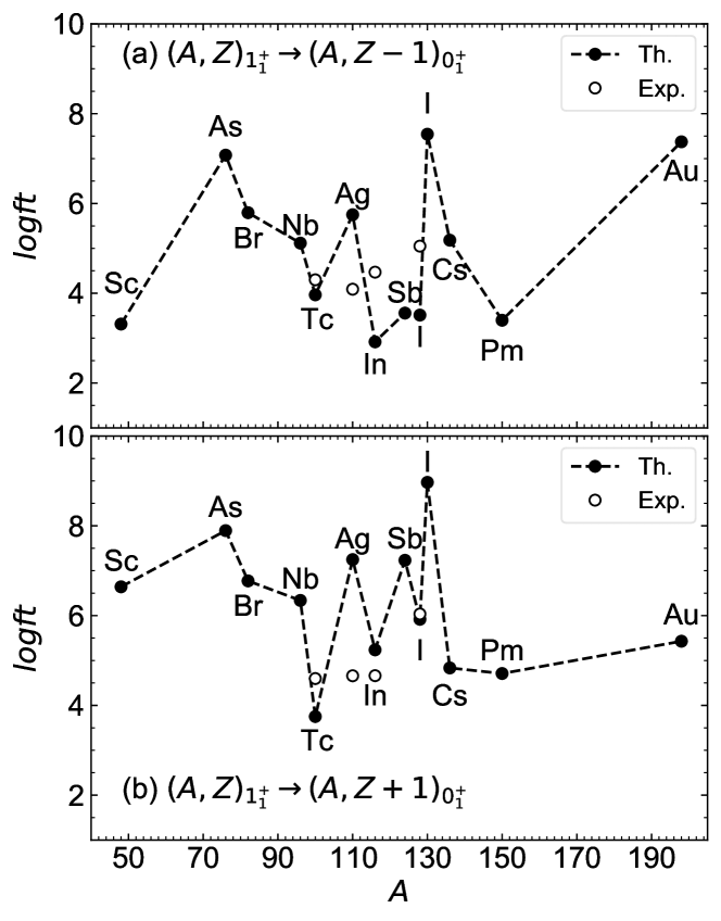
Figure 5: Calculated and experimental [65] $\log{ft}$ values for (a) electron-capture (EC) and (b) $\beta^{-}$ decays from the $1^{+}_{1}$ state of odd-odd nuclei to the ground state $0^{+}_{1}$ of initial- and final-state even-even nuclei, respectively. For the experimental data, error bars are not shown because they are smaller than the marker size.

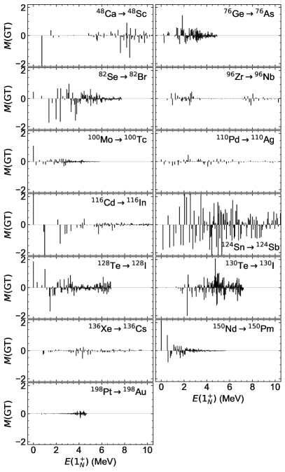
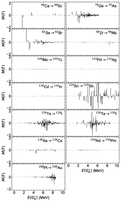
Figure 6: Gamow-Teller $M(\mathrm{GT};0^{+}_{1,I}\to 1^{+}_{N})$ and Fermi $M(\mathrm{F};0^{+}_{1,I}\to 0^{+}_{N})$ matrix elements between the initial and the $N$th intermediate states, plotted against their excitation energies $E(1^{+}_{N})$ and $E(0^{+}_{N})$ (in MeV), respectively.

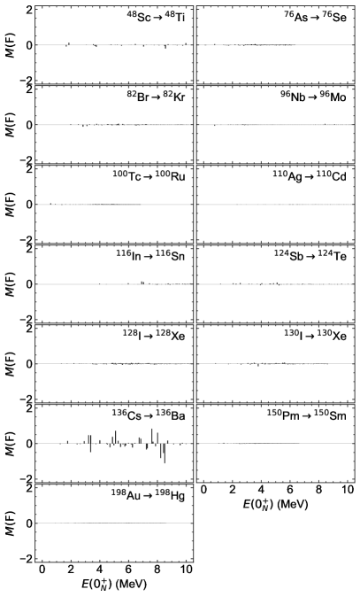
Figure 7: Same as Fig. 6, but for $M(\mathrm{GT};1^{+}_{N}\to 0^{+}_{1,F})$ and $M(\mathrm{F};0^{+}_{N}\to 0^{+}_{1,F})$ between the $N$th intermediate and the final states.

IV Single $\beta$ decay

The $ft$ value for the $\beta$ decay is given by

$$ft=\frac{K}{|M({\mathrm{F}})|^{2}+\left(\frac{g_{\mathrm{A}}}{g_{\mathrm{V}}}\right)^{2}|M({\mathrm{GT}})|^{2}}.$$ (22)

The constant $K=6163$ s, and $M({\mathrm{F}})$ and $M({\mathrm{GT}})$ are the reduced matrix elements of the Fermi $\hat{T}^{\mathrm{F}}$ (17) and Gamow-Teller $\hat{T}^{\mathrm{GT}}$ (18) operators, respectively. For the calculations of single-$\beta$ decays, the free value of the axial vector constant $g_{\mathrm{A}}=1.269$ is used, i.e., no quenching is introduced.

Figure 5 shows the $\log{ft}$ values for (a) $\beta^{+}$ or electron-capture (EC) decays, and (b) $\beta^{-}$ decays of the $1^{+}_{1}$ state of the intermediate odd-odd nuclei into the ground states $0^{+}_{1}$ of the initial and final nuclei, respectively. The obtained $\log{ft}$ values for the EC decay are typically within the range $3\lesssim\log{ft}\lesssim 7$, while the calculated values for the $\beta^{-}$ decays of most of the nuclei are larger than the ones for the EC decays, i.e., $4\lesssim\log{ft}\lesssim 9$. Both the EC and $\beta^{-}$ decay $\log{ft}$ values strongly depend on the mass number $A$.

On closer inspection, the $\log{ft}$ value for the EC decay of the state ¹¹⁶In$(1^{+}_{1})$ is underestimated by a factor of 2. For the ¹¹⁶In nucleus, the neutron-proton pair configuration $[\nu{g_{7/2}}\otimes\pi{g_{9/2}}]^{(J=1)}$ accounts for $84\,\%$ of the IBFFM-2 wave function of the $1^{+}_{1}$ state. This configuration makes a large contribution to the $\pi{g_{9/2}}\leftrightarrow\nu{g_{7/2}}$ transitions in the GT matrix elements, hence the resultant $\log{ft}$ values becomes small, particularly for the EC decay (Fig. 5(a)). The same observation applies to the single-$\beta$ decays of ¹⁰⁰Tc, in which case the predicted $1^{+}_{1}$ wave function turns out to be similar in structure to the one for ¹¹⁶In, i.e., most (86 %) of the $1^{+}_{1}$ wave function for ¹⁰⁰Tc is built on the configuration $[\nu{g_{7/2}}\otimes\pi{g_{9/2}}]^{(J=1)}$. Therefore, the resultant $\log{ft}$ values for the EC and $\beta^{-}$ decays of ¹⁰⁰Tc are relatively small. On the other hand, the $\log{ft}$ values for both the EC and $\beta^{-}$ decays of ¹¹⁰Ag are quite large, as compared to the neighboring nuclei ¹⁰⁰Tc and ¹¹⁶In, and also overestimate the experimental values. In ¹¹⁰Ag, the neutron-proton pair component $[\nu{g_{7/2}}\otimes\pi{g_{9/2}}]^{(J=1)}$ plays a less dominant role than in ¹⁰⁰Tc and ¹¹⁶In, as it constitutes 64 % of the $1^{+}_{1}$ wave function. Consequently, the coupling $\pi{g_{9/2}}\leftrightarrow\nu{g_{7/2}}$ in the GT strengths plays a much less significant role for both the EC and $\beta^{-}$ decays than in the case of the ¹¹⁶In and ¹⁰⁰Tc ones, yielding the large $\log{ft}$ values. The nature of the wave function also appears to be sensitive to the parameters for the IBFFM-2. For ¹⁰⁰Ag, particularly large strength parameter is chosen for the tensor term (see Table 16). It is also worth noticing that the $\log{ft}$ values for both the EC and $\beta^{-}$ decays of ¹³⁰I are quite large. In the corresponding IBFFM-2 wave function of the $1^{+}_{1}$ state, pair components are largely fragmented, with the dominant contributions coming from the $[\nu{s_{1/2}}\otimes\pi{g_{7/2}}]^{(J=3)}$ ($67\,\%$) and $[\nu{d_{3/2}}\otimes\pi{s_{1/2}}]^{(J=2)}$ ($14\,\%$). These configurations do not make any contribution to the GT transition, since the only allowed GT transition in the present case is the one between states with $\ell_{\nu}=\ell_{\pi}$ [see Eq. (19)]. The GT matrix element of the ¹³⁰I decay is also composed of numerous other terms with the amplitudes of small orders of magnitude, which cancel each other, leading to the large $\log{ft}$ values. Cancellations of this kind are supposed to be sensitive to the wave functions of the IBM-2 and IBFFM-2, or the adopted single-particle energies.

In Fig. 6, the distributions of the $M({\mathrm{GT}})$ and $M({\mathrm{F}})$ matrix elements between the initial and the $N$th intermediate states $1^{+}_{N}$ and $0^{+}_{N}$ are shown as functions of their excitation energies below $E_{x}=10$ MeV. In most of the considered decay chains, the $M({\mathrm{GT}};0^{+}_{1,I}\to 1^{+}_{N})$ matrix elements appear to be evenly distributed. The Fermi matrix elements $M({\mathrm{F}};0^{+}_{1,I}\to 0^{+}_{N})$ are also fragmented to a large extent, with generally smaller magnitudes than $M({\mathrm{GT}})$. In some of the decay chains, the $M({\mathrm{F}})$ values almost vanish. For the ¹⁰⁰Mo$\to^{100}$Tc decay, for instance, the only possible transition that contributes to $M({\mathrm{F}})$ is the one between the neutron and proton ${1g_{7/2}}$ orbitals. But the corresponding pair configurations $[\nu{g_{7/2}}\otimes\pi{g_{7/2}}]^{(J)}$ in the IBFFM-2 wave function of the low-lying $0^{+}$ states of ¹⁰⁰Tc are negligibly small, since the proton $1g_{7/2}$ orbital basically belongs to the next major shell to the considered fermion space and its coupling to the neutron $1g_{7/2}$ orbital is weak. (see Table 11).

Figure 7 shows the $M({\mathrm{GT}};1^{+}_{N}\to 0^{+}_{1,F})$ and $M({\mathrm{F}};0^{+}_{N}\to 0^{+}_{1,F})$ matrix elements between the $1^{+}_{N}$ and $0^{+}_{N}$ intermediate states to the final state $0^{+}_{1,F}$. Both the $M({\mathrm{GT}})$ and $M({\mathrm{F}})$ values for these decays are much smaller than in the case of the $\beta^{+}$/EC ones (see Fig. 6). It is remarkable that for the ¹⁰⁰Tc$\to^{100}$Mo and ¹⁵⁰Pm$\to^{150}$Sm $\beta^{-}$ decays, the largest $M({\mathrm{GT}})$ value is obtained at the lowest-lying $1^{+}$ intermediate state.

V $2\nu\beta\beta$ decay

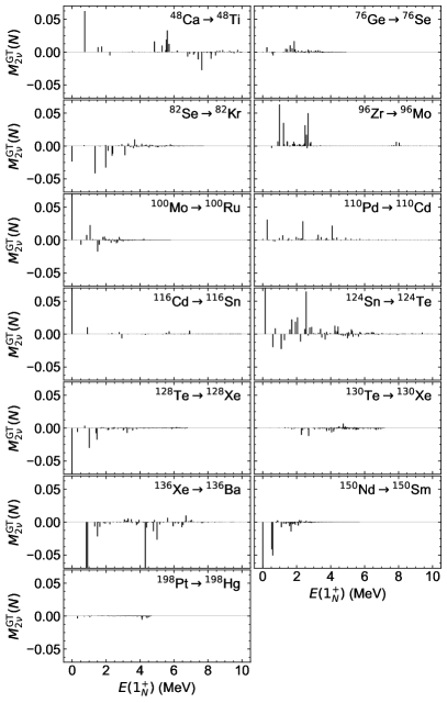
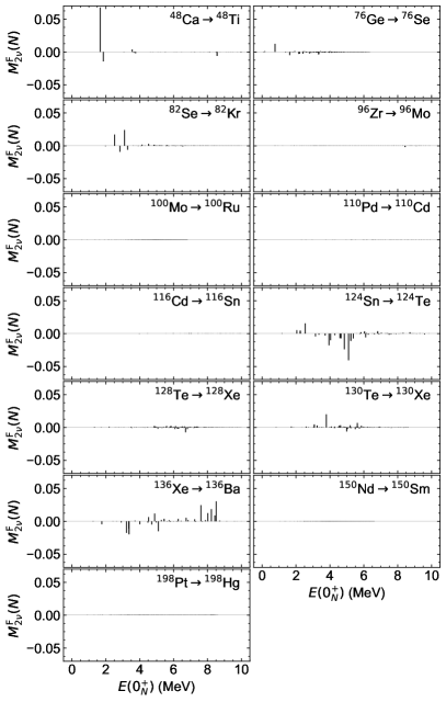
Figure 8: Gamow-Teller $M^{\mathrm{GT}}_{2\nu}(N)$ (25) (first and second columns) and Fermi $M^{\mathrm{F}}_{2\nu}(N)$ (26) (third and fourth columns) matrix elements of the $2\nu\beta\beta$ decays, plotted against $E(1^{+}_{N})$ and $E(0^{+}_{N})$, respectively.

V.1 Estimation of $Q_{\beta\beta}$ values

As shown in the formulas (15) and (16), the $Q_{\beta\beta}$ value is needed for the calculation of the $2\nu\beta\beta$-decay NME. The $Q_{\beta\beta}$ values is here calculated by using the formula

$$Q_{\beta\beta}=2(m_{n}-m_{p}-m_{e})c^{2}+E_{\mathrm{gs}}^{I}-E_{\mathrm{gs}}^{F}$$ (23)

where $m_{n}$, $m_{p}$, and $m_{e}$ are neutron, proton, and electron masses, respectively. $E_{\mathrm{gs}}^{I}$ (or $E_{\mathrm{gs}}^{F}$) stands for the ground-state energy of the IBM-2 for the initial (or final) nucleus, and is given by

$$E_{\mathrm{gs}}=E_{\mathrm{IBM}}(0^{+}_{1})+E_{0},$$ (24)

where the first term stands for the IBM-2 eigenenergy of the $0^{+}_{1}$ ground state and $E_{0}$ is a constant term that depends on nucleon numbers but does not affect excitation energies [72]. For each of the initial and final nuclei, the constant $E_{0}$ is equated to the total mean-field energy at the spherical configuration, $E_{\mathrm{SCMF}}(0,\gamma)$ (see Ref. [67] for details). One further needs the $Q$ value of the $\beta^{-}$ decay of the initial nucleus. It could also be determined by using the eigenenergies of the IBM-2 and IBFFM-2, and the total SCMF energies. However, the calculation of the $Q_{\beta}$ value of odd-odd nucleus within the present framework would be complicated, since it is strongly influenced by the combinations of a number of parameters for the IBFFM-2. In order to simplify the discussion, here the experimental $Q_{\beta}$ values taken from [65] are employed.

Table 2: Calculated and experimental $Q_{\beta\beta}$ values (in MeV) of initial even-even nuclei, denoted by $Q_{\beta\beta,\mathrm{th}}$ and $Q_{\beta\beta,\mathrm{ex}}$, respectively. The $Q_{\beta\beta,\mathrm{ex}}$ values are taken from Ref. [65]. The $Q_{\beta}$ values of the initial nuclei, adopted from the data [65], are also shown.

Nucleus	$Q_{\beta\beta,\mathrm{th}}$ (MeV)	$Q_{\beta\beta,\mathrm{ex}}$ (MeV)	$Q_{\beta}$ (MeV)
48Ca	$1.8479$	$4.2681$	$0.2790$
76Ge	$0.8831$	$2.0391$	$0.9215$
82Se	$1.6356$	$2.9979$	$0.0952$
96Zr	$4.1285$	$3.3560$	$0.1640$
100Mo	$2.8338$	$3.0344$	$0.1721$
110Pd	$2.9081$	$2.0171$	$0.8736$
116Cd	$6.1166$	$2.8135$	$0.4627$
124Sn	$-0.3795$	$2.2927$	$0.6124$
128Te	$-0.1784$	$0.8680$	$1.2518$
130Te	$1.4466$	$2.5290$	$0.4200$
136Xe	$0.0989$	$2.4579$	$0.0903$
150Nd	$3.3123$	$3.3714$	$0.0830$
198Pt	$1.2895$	$1.0503$	$0.3232$

Table 2 shows the calculated and experimental [65] $Q_{\beta\beta}$ values, denoted by $Q_{\beta\beta,\mathrm{th}}$ and $Q_{\beta\beta,\mathrm{ex}}$, respectively. The $Q_{\beta\beta,\mathrm{th}}$ values for many of the nuclei are close to the experimental ones, whereas negative $Q_{\beta\beta}$ values are obtained for ¹²⁴Sn and ¹²⁸Te. The calculation of the $Q_{\beta\beta}$ value depends on a subtle balance between the SCMF total energies for the initial and final nuclei, as well as between the eigenenergies of the IBM-2. Note that, as for ¹²⁸Te, the deformed QRPA calculation for $\beta\beta$ decay with a Skyrme interaction also obtained the negative $Q_{\beta\beta}$ value [73]. In what follows, the results obtained from both $Q_{\beta\beta,\mathrm{th}}$ and $Q_{\beta\beta,\mathrm{ex}}$ values are discussed.

V.2 GT and F matrix elements

One can study strength distributions of each terms in the sums in the $M^{\mathrm{GT}}_{2\nu}$ (15) and $M^{\mathrm{F}}_{2\nu}$ (16) matrix elements, i.e.,

$$M^{\mathrm{GT}}_{2\nu}(N)\equiv\frac{\braket{0^{+}_{F}}{t^{+}\sigma}{1^{+}_{N}}\braket{1^{+}_{N}}{t^{+}\sigma}{0^{+}_{1,I}}}{E_{N}-E_{I}+\frac{1}{2}(Q_{\beta\beta}+2m_{e}c^{2})}$$ (25)

$$M^{\mathrm{F}}_{2\nu}(N)\equiv\frac{\braket{0^{+}_{F}}{t^{+}}{0^{+}_{N}}\braket{0^{+}_{N}}{t^{+}}{0^{+}_{1,I}}}{E_{N}-E_{I}+\frac{1}{2}(Q_{\beta\beta}+2m_{e}c^{2})}.$$ (26)

The corresponding results for the ground-state-to-ground-state ($0^{+}_{1}\to 0^{+}_{1}$) transitions are shown in Fig. 8 as functions of the excitation energies of the $N$th intermediate states $1^{+}_{N}$ and $0^{+}_{N}$. In the figure, only the results that employ the theoretical $Q_{\beta\beta}$ values, i.e., $Q_{\beta\beta,\mathrm{th}}$, calculated by using the formulas (23) and (24), are considered, since there is no striking difference between the results using the $Q_{\beta\beta,\mathrm{th}}$ and $Q_{\beta\beta,\mathrm{ex}}$ values at the qualitative level.

From Fig. 8, for most of the decays, the low-lying $1^{+}$ states appear to make dominant contributions to the GT transitions. This finding more or less conforms to the single-state dominance (SSD) [74, 75] or low-lying state dominance (LLSD) [76] hypotheses. In the earlier IBFFM-2 calculation of Ref. [21], the authors found more distinct SSD nature in the GT strength distributions of the ¹²⁸Te and ¹³⁰Te $2\nu\beta\beta$ decays. One sees in Fig. 8 that the Fermi contributions are generally weak, except for the ⁴⁸Ca, ¹²⁴Sn, and ¹³⁶Xe decays, and their strength distributions do not exhibit a characteristic trend as in the case of the GT ones $M^{\mathrm{GT}}_{2\nu}$.

Table 3 gives the results for Gamow-Teller $M^{\mathrm{GT}}_{2\nu}$ and Fermi $M^{\mathrm{F}}_{2\nu}$ matrix elements for the $0^{+}_{1}\to 0^{+}_{1}$ transition and the ground-state-to-first-excited-state ($0^{+}_{1}\to 0^{+}_{2}$) transition. For the $0^{+}_{1}\to 0^{+}_{1}$ transitions, in most cases the calculated values $|M^{\mathrm{GT}}_{2\nu}(0^{+}_{1}\to 0^{+}_{1})|\approx 0.05-0.15$, while particularly large $M^{\mathrm{GT}}_{2\nu}(0^{+}_{1}\to 0^{+}_{1})$ values are obtained for the ¹⁰⁰Mo and ¹⁵⁰Nd decays. There is also no significant difference in the results for the $M^{\mathrm{GT}}_{2\nu}$ and $M^{\mathrm{F}}_{2\nu}$ matrix elements between the calculations with the $Q_{\beta\beta,\mathrm{th}}$ and $Q_{\beta\beta,\mathrm{ex}}$ values. As for the $0^{+}_{1}\to 0^{+}_{2}$ decays, on the other hand, the prediction of $M^{\mathrm{GT}}_{2\nu}$ and $M^{\mathrm{F}}_{2\nu}$ depends strongly on the choice of the $Q_{\beta\beta}$ values, particularly for the ⁴⁸Ca, ¹²⁴Sn, and ¹³⁶Xe decays. Indeed, the corresponding $Q_{\beta\beta,\mathrm{th}}$ values for these processes are quite different from the experimental ones $Q_{\beta\beta,\mathrm{ex}}$ (see Table 2). These nuclei are also all doubly or semimagic nuclei, for which the IBM framework is not considered a very good approach to give a reasonable $Q_{\beta\beta}$ value. In addition, both the calculated $M^{\mathrm{GT}}_{2\nu}$ and $M^{\mathrm{F}}_{2\nu}$ values for certain $0^{+}_{1}\to 0^{+}_{2}$ transitions, i.e., ⁴⁸Ca$\to^{48}$Ti, ⁷⁶Ge$\to^{76}$Se, and ⁸²Se$\to^{82}$Kr, are much larger in magnitude than those for the $0^{+}_{1}\to 0^{+}_{1}$ transitions, especially when the $Q_{\beta\beta,\mathrm{th}}$ values are used.

Table 3: Calculated Gamow-Teller $M^{\mathrm{GT}}_{2\nu}$ (15) and Fermi $M^{\mathrm{F}}_{2\nu}$ (16) matrix elements for the $0^{+}_{1}\to 0^{+}_{1}$ and $0^{+}_{1}\to 0^{+}_{2}$ $2\nu\beta\beta$ decays. Each matrix element is presented for the two cases in which the experimental [65] and theoretical $Q_{\beta\beta}$ values, represented by $Q_{\beta\beta,\mathrm{ex}}$ and $Q_{\beta\beta,\mathrm{th}}$, respectively, are used [see Table 2 and Eq. (24)].

Decay	$0^{+}_{1}$				$0^{+}_{2}$
	$M^{\mathrm{GT}}_{2\nu}$		$M^{\mathrm{F}}_{2\nu}$		$M^{\mathrm{GT}}_{2\nu}$		$M^{\mathrm{F}}_{2\nu}$
	$Q_{\beta\beta,\mathrm{th}}$	$Q_{\beta\beta,\mathrm{ex}}$	$Q_{\beta\beta,\mathrm{th}}$	$Q_{\beta\beta,\mathrm{ex}}$	$Q_{\beta\beta,\mathrm{th}}$	$Q_{\beta\beta,\mathrm{ex}}$	$Q_{\beta\beta,\mathrm{th}}$	$Q_{\beta\beta,\mathrm{ex}}$
48Ca$\to^{48}$Ti	$0.060$	$0.042$	$0.024$	$0.016$	$0.325$	$0.066$	$-0.142$	$-0.075$
76Ge$\to^{76}$Se	$0.040$	$0.034$	$-0.007$	$-0.007$	$0.097$	$0.078$	$-0.085$	$-0.069$
82Se$\to^{82}$Kr	$-0.060$	$-0.045$	$0.017$	$0.015$	$0.124$	$0.070$	$-0.081$	$-0.064$
96Zr$\to^{96}$Mo	$0.139$	$0.154$	$-0.001$	$-0.001$	$0.053$	$0.063$	$-0.000$	$-0.000$
100Mo$\to^{100}$Ru	$0.513$	$0.483$	$-0.000$	$-0.000$	$-0.007$	$-0.020$	$0.000$	$0.000$
110Pd$\to^{110}$Cd	$0.071$	$0.080$	$0.000$	$0.000$	$-0.052$	$-0.062$	$0.000$	$0.000$
116Cd$\to^{116}$Sn	$0.148$	$0.275$	$0.001$	$0.001$	$0.032$	$-0.037$	$-0.001$	$-0.001$
124Sn$\to^{124}$Te	$0.123$	$0.074$	$-0.054$	$-0.045$	$0.345$	$-0.066$	$0.016$	$0.012$
128Te$\to^{128}$Xe	$-0.139$	$-0.102$	$0.006$	$0.005$	$0.108$	$0.032$	$0.002$	$0.002$
130Te$\to^{130}$Xe	$-0.041$	$-0.037$	$0.025$	$0.022$	$0.043$	$0.037$	$-0.019$	$-0.017$
136Xe$\to^{136}$Ba	$-0.173$	$-0.102$	$0.028$	$0.028$	$-2.807$	$0.010$	$0.009$	$0.001$
150Nd$\to^{150}$Sm	$-0.375$	$-0.369$	$0.000$	$0.000$	$-0.414$	$-0.390$	$-0.000$	$-0.000$
198Pt$\to^{198}$Hg	$-0.016$	$-0.016$	$0.001$	$0.001$	$-0.008$	$-0.010$	$-0.000$	$-0.000$

Table 4: Ratio of the calculated $M^{\mathrm{F}}_{2\nu}$ to $M^{\mathrm{GT}}_{2\nu}$ matrix elements $\chi_{F}(0^{+})=M^{\mathrm{F}}_{2\nu}/M^{\mathrm{GT}}_{2\nu}$ for the $0^{+}_{1}\to 0^{+}_{1}$ and $0^{+}_{1}\to 0^{+}_{2}$ $2\nu\beta\beta$ decays of the even-even nuclei under investigation in the cases where the two different $Q_{\beta\beta}$ values, $Q_{\beta\beta,\mathrm{th}}$ and $Q_{\beta\beta,\mathrm{ex}}$, are used.

Nucleus	$Q_{\beta\beta,\mathrm{th}}$		$Q_{\beta\beta,\mathrm{ex}}$
	$\chi_{F}(0^{+}_{1})$	$\chi_{F}(0^{+}_{2})$	$\chi_{F}(0^{+}_{1})$	$\chi_{F}(0^{+}_{2})$
48Ca	$0.401$	$-0.435$	$0.390$	$-1.147$
76Ge	$-0.179$	$-0.874$	$-0.204$	$-0.888$
82Se	$-0.287$	$-0.650$	$-0.328$	$-0.923$
96Zr	$-0.006$	$-0.003$	$-0.005$	$-0.002$
100Mo	$-0.000$	$-0.005$	$-0.000$	$-0.002$
110Pd	$0.000$	$-0.000$	$0.000$	$-0.000$
116Cd	$0.004$	$-0.021$	$0.002$	$0.022$
124Sn	$-0.443$	$0.046$	$-0.608$	$-0.182$
128Te	$-0.040$	$0.016$	$-0.051$	$0.050$
130Te	$-0.104$	$-0.093$	$-0.601$	$-0.460$
136Xe	$-0.163$	$-0.003$	$-0.278$	$0.061$
150Nd	$-0.001$	$0.000$	$-0.001$	$0.000$
198Pt	$-0.060$	$0.036$	$-0.059$	$0.030$

As one can see in Table 3, for both the $0^{+}_{1}\to 0^{+}_{1}$ and $0^{+}_{1}\to 0^{+}_{2}$ decays, the Fermi NMEs $M^{\mathrm{F}}_{2\nu}$ are, as a whole, calculated to be smaller in magnitude than the GT ones, $M^{\mathrm{GT}}_{2\nu}$. However, for those even-even nuclei where protons and neutrons can occupy the same major shells, i.e., ⁴⁸Ca, ⁷⁶Ge, ⁸²Se, ¹²⁴Sn, ^128,130Te, and ¹³⁶Xe, the corresponding $M^{\mathrm{F}}_{2\nu}$ matrix elements are of the same order of magnitude as the $M^{\mathrm{GT}}_{2\nu}$ ones. In particular, for ⁴⁸Ca the calculated $|M^{\mathrm{F}}_{2\nu}(0^{+}_{1}\to 0^{+}_{2})|$ value is even larger than the $|M^{\mathrm{GT}}_{2\nu}(0^{+}_{1}\to 0^{+}_{2})|$ one. This finding is further corroborated by the Fermi strength distribution systematics shown in Fig. 8, in which non-negligible contributions of the Fermi transition are already apparent for the ⁴⁸Ca, ¹²⁴Sn, and ¹³⁶Xe decays.

To examine more quantitatively the contribution of the Fermi transition relative to the GT one, the ratio $\chi_{F}\equiv M^{\mathrm{F}}_{2\nu}/M^{\mathrm{GT}}_{2\nu}$ [6] is calculated for the $2\nu\beta\beta$ decays of interest. The results are listed in Table 4. If the isospin is a good symmetry quantum number, the ratio $\chi_{F}$ should be equal to zero. For the $2\nu\beta\beta$ decay mode, the Fermi matrix element should vanish, while in the $0\nu\beta\beta$ decay it is expected to be non-vanishing but also quite small. The large $M^{\mathrm{F}}_{2\nu}$ matrix element or $\chi_{F}$ ratio therefore implies that there is a spurious isospin-symmetry breaking in the wave functions of the initial and final even-even nuclei generated by the employed model. For the aforementioned even-even nuclei ⁴⁸Ca, ⁷⁶Ge, ⁸²Se, ¹²⁴Sn, ^128,130Te, and ¹³⁶Xe, the ratio $|\chi_{F}|$ is here calculated to be substantially large, which is typically $|\chi_{F}|\gtrsim 0.1$. One further observes in Table 4 that, in general, the calculation with the experimental $Q_{\beta\beta}$ values, $Q_{\beta\beta,\mathrm{ex}}$, leads to a larger degree of the isospin symmetry breaking than with the theoretical $Q_{\beta\beta}$ values, $Q_{\beta\beta,\mathrm{th}}$. A similar degree of isospin symmetry breaking to the present case was reported in the earlier IBM-2 calculations in Refs. [42, 21]. The problem was addressed in great detail in Refs. [42, 43]. In Ref. [43], in particular, a method to restore the broken isospin symmetry in the calculation of the Fermi matrix element for the $2\nu\beta\beta$ decay was proposed, that is to modify the Fermi transition operator so that the Fermi matrix element within the closure approximation should vanish.

In the present theoretical framework, provided that the Fermi transition is actually spurious, then either the Fermi contribution $M^{\mathrm{F}}_{2\nu}$ would have to be simply neglected, or some modification should be made to the Fermi transition operator of (17) in a similar spirit to Ref. [43]. The latter prescription points to an interesting question as to how the broken isospin symmetry can be treated in the mapped IBM-2 framework, but is at the same time beyond the scope of the present investigation. In the following, the Fermi matrix element is retained in the calculation of the $2\nu\beta\beta$-decay NME, while it should be kept in mind that especially for those nuclei with approximately equal proton and neutron numbers a spurious isospin symmetry breaking may be present in the large Fermi matrix element.

V.3 $2\nu\beta\beta$ NMEs

In the second and fifth columns of Table 5, the results for the $2\nu\beta\beta$ NMEs are given. In the last column, the effective NMEs denoted by $M_{2\nu}^{\mathrm{eff}}$, which are extracted from the observed $2\nu\beta\beta$-decay half-lives [12], are also shown. The calculated NMEs are typically within the range $0.05\lesssim|M_{2\nu}|\lesssim 0.3$, which are in most cases larger than the experimental values $|M_{2\nu}^{\mathrm{eff}}|$. For the $0^{+}_{1}\to 0^{+}_{1}$ decays of ¹⁰⁰Mo, and both the $0^{+}_{1}\to 0^{+}_{1}$ and $0^{+}_{1}\to 0^{+}_{2}$ decays of ¹⁵⁰Nd, the corresponding $M_{2\nu}$ are particularly large.

Table 5: Calculated $2\nu\beta\beta$-decay NMEs $M_{2\nu}$ (14) (second and fifth columns), and $M_{2\nu}^{\mathrm{(I)}}$ (third and sixth columns) and $M_{2\nu}^{\mathrm{(II)}}$ (fourth and seventh columns), quenched with the effective $g_{\mathrm{A}}$ factors $g_{\mathrm{A,eff}}^{\mathrm{(I)}}$ (28) and $g_{\mathrm{A,eff}}^{\mathrm{(II)}}$ (29), respectively. The results obtained with the theoretical and experimental $Q_{\beta\beta}$ values are compared. The effective NMEs $M_{2\nu}^{\mathrm{eff}}$ extracted from the $\tau_{1/2}^{(2\nu)}$ data [12] are shown in the eighth column.

Decay	$Q_{\beta\beta,\mathrm{th}}$			$Q_{\beta\beta,\mathrm{ex}}$			$|M_{2\nu}^{\mathrm{eff}}|$ [12]
	$|M_{2\nu}|$	$|M_{2\nu}^{\mathrm{(I)}}|$	$|M_{2\nu}^{\mathrm{(II)}}|$	$|M_{2\nu}|$	$|M_{2\nu}^{\mathrm{(I)}}|$	$|M_{2\nu}^{\mathrm{(II)}}|$
48Ca$\to^{48}$Ti	0.073	0.020	0.034	0.051	0.014	0.024	$0.035\pm 0.003$
76Ge$\to^{76}$Se	0.072	0.017	0.021	0.062	0.014	0.018	$0.106\pm 0.004$
82Se$\to^{82}$Kr	0.115	0.026	0.031	0.087	0.020	0.024	$0.085\pm 0.001$
96Zr$\to^{96}$Mo	0.225	0.048	0.048	0.249	0.053	0.054	$0.088\pm 0.004$
100Mo$\to^{100}$Ru	0.827	0.174	0.167	0.778	0.164	0.157	$0.185\pm 0.002$
100Mo$\to^{100}$Ru$(0^{+}_{2})$	0.011	0.002	0.002	0.032	0.007	0.007	$0.151\pm 0.004$
110Pd$\to^{110}$Cd	0.115	0.023	0.020	0.128	0.026	0.022
116Cd$\to^{116}$Sn	0.238	0.048	0.037	0.443	0.089	0.069	$0.108\pm 0.003$
124Sn$\to^{124}$Te	0.253	0.050	0.035	0.164	0.032	0.022
128Te$\to^{128}$Xe	0.229	0.044	0.030	0.169	0.033	0.022	$0.043\pm 0.003$
130Te$\to^{130}$Xe	0.091	0.017	0.011	0.081	0.016	0.010	$0.0293\pm 0.0009$
136Xe$\to^{136}$Ba	0.307	0.058	0.035	0.194	0.037	0.022	$0.0181\pm 0.0006$
150Nd$\to^{150}$Sm	0.604	0.111	0.055	0.594	0.109	0.054	$0.055\pm 0.003$
150Nd$\to^{150}$Sm$(0^{+}_{2})$	0.666	0.122	0.060	0.629	0.116	0.057	$0.044\pm 0.005$
198Pt$\to^{198}$Hg	0.026	0.004	0.001	0.027	0.005	0.001

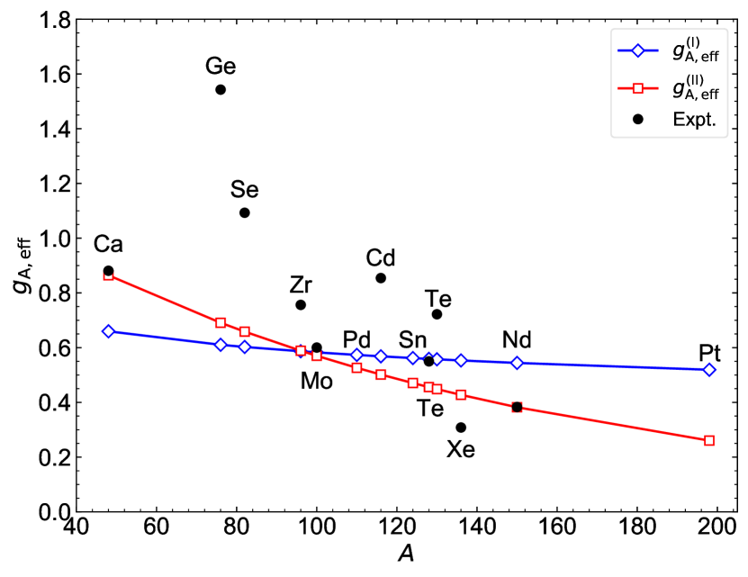
Figure 9: Effective $g_{\mathrm{A}}$ factors $g_{\mathrm{A,eff}}^{\mathrm{(I)}}=g_{\mathrm{A}}{A}^{-0.169}$ (28) (diamonds) and $g_{\mathrm{A,eff}}^{\mathrm{(II)}}=g_{\mathrm{A}}e^{-0.008A}$ (29) (squares). The solid circles denoted by “Expt.” represent $g_{\mathrm{A,eff}}$ values that would be required to reproduce the experimental NMEs $M_{2\nu}^{\mathrm{eff}}$.

To make a reasonable comparison with experiment, one can consider quenching of the obtained NME. Here it is assumed that in Eq. (14) only the $g_{\mathrm{A}}$ factor is quenched, whereas the ratio $g_{\mathrm{V}}/g_{\mathrm{A}}$, as well as $g_{\mathrm{V}}$, is not. The quenched NME can be then obtained by simply replacing the free value $g_{\mathrm{A}}$ in (14) with the effective $g_{\mathrm{A}}$ factor denoted by $g_{\mathrm{A,eff}}$, i.e.,

$$|M_{2\nu}|\rightarrow\left(\frac{g_{\mathrm{A,eff}}}{g_{\mathrm{A}}}\right)^{2}|M_{2\nu}|.$$ (27)

Also the quenching factor $q$ is given by $q=g_{\mathrm{A,eff}}/g_{\mathrm{A}}$. It is further assumed that the $g_{\mathrm{A,eff}}$ factor is a smooth function of the mass number $A$, and specifically the two parametrizations are here considered:

$$g_{\mathrm{A,eff}}^{\mathrm{(I)}}=g_{\mathrm{A}}\cdot{A}^{-a},$$ (28)

$$g_{\mathrm{A,eff}}^{\mathrm{(II)}}=g_{\mathrm{A}}\cdot{e^{-bA}}.$$ (29)

The numerical constants $a=0.169$ and $b=0.008$ are obtained by fitting to those $g_{\mathrm{A,eff}}$ values that would be required to reproduce the $M_{2\nu}^{\mathrm{eff}}(0^{+}_{1}\to 0^{+}_{1})$ values. At $A\approx 1$, both $g_{\mathrm{A,eff}}^{\mathrm{(I)}}$ and $g_{\mathrm{A,eff}}^{\mathrm{(II)}}$ reduce to the free nucleon value $g_{\mathrm{A}}=1.269$. A similar parametrization to the first choice (28) was considered in the previous IBM-2 study on the $\beta\beta$ decay [42]. The constant $a=0.169$ is also close to the one ($0.18$) used in the above reference.

The resultant $g_{\mathrm{A,eff}}^{\mathrm{(I)}}$ and $g_{\mathrm{A,eff}}^{\mathrm{(II)}}$ values are shown in Fig. 9 as functions of $A$. The $g_{\mathrm{A,eff}}^{\mathrm{(I)}}$ value only gradually changes with $A$ within the range $0.5\lesssim g_{\mathrm{A,eff}}^{\mathrm{(I)}}\lesssim 0.7$, corresponding to the quenching factor of $q\approx 0.4-0.5$. The second choice, $g_{\mathrm{A,eff}}^{\mathrm{(II)}}$, takes more or less similar values to $g_{\mathrm{A,eff}}^{\mathrm{(I)}}$ in the mass range $A\approx 100-130$, but is smaller for heavier nuclei, giving rise to a more drastic quenching than $g_{\mathrm{A,eff}}^{\mathrm{(I)}}$. For the ⁷⁶Ge and ⁸²Se decays, the present $g_{\mathrm{A,eff}}$ factors of both choices (28) and (29) are still much smaller than those that would be required to reproduce the $M_{2\nu}^{\mathrm{eff}}$ values. In fact, one sees in Table 5 that even before the quenching the corresponding $M_{2\nu}$ is smaller than the data for ⁷⁶Ge, and that is already close to the experimental value for ⁸²Se. From these observations, the present $g_{\mathrm{A,eff}}$ values for the above two particular cases might not be adequate.

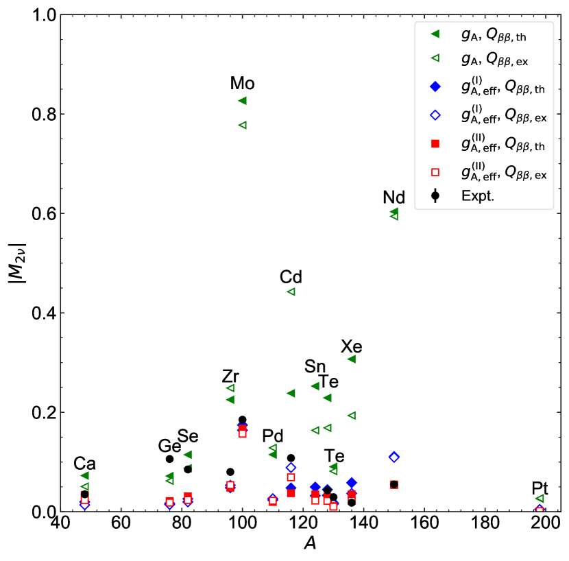
Figure 10: $0^{+}_{1}\to 0^{+}_{1}$ $2\nu\beta\beta$-decay NMEs $M_{2\nu}$ (14) (triangles), and quenched NMEs $M_{2\nu}^{\mathrm{(I)}}$ (diamonds) and $M_{2\nu}^{\mathrm{(II)}}$ (squares), using the effective $g_{\mathrm{A}}$ factors $g_{\mathrm{A,eff}}^{\mathrm{(I)}}$ and $g_{\mathrm{A,eff}}^{\mathrm{(II)}}$, respectively. The results obtained with the theoretical $Q_{\beta\beta,\mathrm{th}}$ (filled symbols) and experimental $Q_{\beta\beta,\mathrm{ex}}$ (open symbols) values are compared. The solid circles represent the experimental NMEs or $M_{2\nu}^{\mathrm{eff}}$.

In the third, fourth, sixth, and seventh columns of Table 5 listed are the values of the quenched NMEs, denoted as $M_{2\nu}^{\mathrm{(I)}}$ and $M_{2\nu}^{\mathrm{(II)}}$, obtained by using the two different choices of the effective $g_{\mathrm{A}}$ factor $g_{\mathrm{A,eff}}^{\mathrm{(I)}}$ (28) and $g_{\mathrm{A,eff}}^{\mathrm{(II)}}$ (29), respectively. The quenched NMEs, $M_{2\nu}^{\mathrm{(I)}}$ and $M_{2\nu}^{\mathrm{(II)}}$, are both close to the experimental data. In general, the second choice $g_{\mathrm{A,eff}}^{\mathrm{(II)}}$ (29) appears to give a better agreement with experiment than the first one, $g_{\mathrm{A,eff}}^{\mathrm{(I)}}$ (28). A specific comment concerns that, for the ⁷⁶Ge and ⁸²Se decays, the quenching reduces too much the NMEs and only worsens the agreement with the experimental values, as compared to the unquenched NMEs. In addition, the NME for the ¹⁰⁰Mo$\to^{100}$Ru$(0^{+}_{2})$ decay is considerably underestimated even without the quenching, irrespective of whether the $Q_{\beta\beta,\mathrm{th}}$ or $Q_{\beta\beta,\mathrm{ex}}$ values is used. This may suggest that there are some missing elements in the calculation for the final nucleus ¹⁰⁰Ru such as the intruder excitations, which may be needed to give a correct wave function for the $0^{+}_{2}$ state. For completeness, in Fig. 10 the values of the $2\nu\beta\beta$-decay NMEs for the $0^{+}_{1}\to 0^{+}_{1}$ decay, that are already listed in Table 5, are shown in comparison with the experimental values $M_{2\nu}^{\mathrm{eff}}$.

Alternatively, one can extract the $g_{\mathrm{A,eff}}$ values for the $2\nu\beta\beta$ decay from the single-$\beta$ decay data. This can be done by fitting the calculated $\beta$-decay $\log{ft}$ values to the experimental counterparts. Consider the $2\nu\beta\beta$ decay of ¹⁰⁰Mo an an illustrative example. This is an ideal case, in which the GT transitions for the single-$\beta$ and $\beta\beta$ decays of the intermediate nucleus is dominated by the transitions from the lowest $1^{+}$ state [see, Figs. 6–8]. For this decay chain, the $g_{\mathrm{A,eff}}$ values are calculated to be $g_{\mathrm{A,eff,\beta}}=0.863$ and $g_{\mathrm{A,eff,\beta}}=0.479$ for the EC and $\beta^{-}$ decays of the state ¹⁰⁰Tc$\,(1^{+}_{1})$, respectively. If their average $0.671$ is used as the effective $g_{\mathrm{A,eff}}$ for the $2\nu\beta\beta$ decay, then the corresponding NME $M_{2\nu}$ is quenched to $0.231$, in a fair agreement with the $M_{2\nu}^{\mathrm{(I)}}$ and $M_{2\nu}^{\mathrm{(II)}}$ values shown in Table 5. A similar result is obtained for the ¹²⁸Te decay. In most of the other cases, however, as one sees in Figs. 6–8 the GT matrix elements for both the single-$\beta$ and $\beta\beta$ decays are not as sharply populated at the lowest $1^{+}$ state as in the case of the ¹⁰⁰Mo$\to^{100}$Ru or ¹²⁸Te$\to^{128}$Xe ones. Furthermore, the present calculation for single-$\beta$ decays, which uses the free value for the $g_{\mathrm{A}}$ factor, generally gives larger $\log{ft}$ values for the EC processes of the intermediate nuclei. Experimental $\log{ft}$ values for the $\beta^{-}$ decay are also not available, except for ¹⁰⁰Tc, ¹¹⁰Ag, ¹¹⁶In, and ¹²⁸I. For these reasons, within the present theoretical scheme, the prescription to extract $\beta\beta$-decay $g_{\mathrm{A,eff}}$ factors from the single-$\beta$ decays is not expected to give a reasonable agreement of the $2\nu\beta\beta$ NME with experiment in a systematic way.

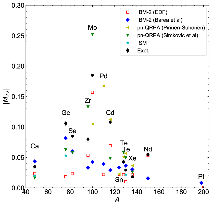
Figure 11: Calculated $2\nu\beta\beta$-decay NMEs (14) in the present study [denoted by “IBM-2 (EDF)”], obtained with the effective $g_{\mathrm{A}}$ factor $g_{\mathrm{A,eff}}^{\mathrm{(II)}}$ and with the $Q_{\beta\beta,\mathrm{ex}}$ values. The experimental NMEs ($M_{2\nu}^{\mathrm{eff}}$) and those obtained from the proton-neutron QRPA (pn-QRPA) by Šimković et al. [14] and Pirinen and Suhonen [13], from the IBM-2 by Barea et al. [43], and from the ISM by Caurier et al. [15] are also shown.

Table 6: Comparison of calculated $2\nu\beta\beta$-decay half-lives $\tau_{1/2}^{(2\nu)}$ (in year) corresponding to the free value of the $g_{\mathrm{A}}$ factor, and the effective values $g_{\mathrm{A,eff}}^{\mathrm{(I)}}$ (28) and $g_{\mathrm{A,eff}}^{\mathrm{(II)}}$ (29) factors, in two difference cases of the $Q_{\beta\beta}$ values, $Q_{\beta\beta,\mathrm{th}}$ (second to fourth columns) and $Q_{\beta\beta,\mathrm{ex}}$ (fifth to seventh columns). The experimental values taken from Ref. [12] are shown in the eighth column.

Decay	$\tau_{1/2}^{(2\nu)}$ (yr), with $Q_{\beta\beta,\mathrm{th}}$			$\tau_{1/2}^{(2\nu)}$ (yr), with $Q_{\beta\beta,\mathrm{ex}}$			Expt. [12]
	$g_{\mathrm{A}}$	$g_{\mathrm{A,eff}}^{\mathrm{(I)}}$	$g_{\mathrm{A,eff}}^{\mathrm{(II)}}$	$g_{\mathrm{A}}$	$g_{\mathrm{A,eff}}^{\mathrm{(I)}}$	$g_{\mathrm{A,eff}}^{\mathrm{(II)}}$
48Ca$\to^{48}$Ti	$1.22\times 10^{19}$	$1.67\times 10^{20}$	$5.66\times 10^{19}$	$2.50\times 10^{19}$	$3.43\times 10^{20}$	$1.16\times 10^{20}$	$5.3^{+1.2}_{-0.8}\times 10^{19}$
76Ge$\to^{76}$Se	$4.04\times 10^{21}$	$7.54\times 10^{22}$	$4.59\times 10^{22}$	$5.39\times 10^{21}$	$1.01\times 10^{23}$	$6.14\times 10^{22}$	$(1.88\pm 0.08)\times 10^{21}$
82Se$\to^{82}$Kr	$4.77\times 10^{19}$	$9.38\times 10^{20}$	$6.58\times 10^{20}$	$8.20\times 10^{19}$	$1.61\times 10^{21}$	$1.13\times 10^{21}$	$(0.87^{+0.02}_{-0.01})\times 10^{20}$
96Zr$\to^{96}$Mo	$2.89\times 10^{18}$	$6.32\times 10^{19}$	$6.24\times 10^{19}$	$2.37\times 10^{18}$	$5.19\times 10^{19}$	$5.12\times 10^{19}$	$(2.3\pm 0.2)\times 10^{19}$
100Mo$\to^{100}$Ru	$4.42\times 10^{17}$	$9.95\times 10^{18}$	$1.09\times 10^{19}$	$5.00\times 10^{17}$	$1.12\times 10^{19}$	$1.23\times 10^{19}$	$(7.06^{+0.15}_{-0.13})\times 10^{18}$
100Mo$\to^{100}$Ru$(0^{+}_{2})$	$1.29\times 10^{23}$	$2.91\times 10^{24}$	$3.17\times 10^{24}$	$1.59\times 10^{22}$	$3.57\times 10^{23}$	$3.90\times 10^{23}$	$6.7^{+0.5}_{-0.4}\times 10^{20}$
110Pd$\to^{110}$Cd	$5.51\times 10^{20}$	$1.32\times 10^{22}$	$1.86\times 10^{22}$	$4.40\times 10^{20}$	$1.06\times 10^{22}$	$1.49\times 10^{22}$
116Cd$\to^{116}$Sn	$6.37\times 10^{18}$	$1.58\times 10^{20}$	$2.61\times 10^{20}$	$1.85\times 10^{18}$	$4.59\times 10^{19}$	$7.56\times 10^{19}$	$(2.69\pm 0.09)\times 10^{19}$
124Sn$\to^{124}$Te	$2.83\times 10^{19}$	$7.37\times 10^{20}$	$1.50\times 10^{21}$	$6.76\times 10^{19}$	$1.76\times 10^{21}$	$3.57\times 10^{21}$
128Te$\to^{128}$Xe	$7.09\times 10^{22}$	$1.89\times 10^{24}$	$4.26\times 10^{24}$	$1.31\times 10^{23}$	$3.48\times 10^{24}$	$7.86\times 10^{24}$	$(2.25\pm 0.09)\times 10^{24}$
130Te$\to^{130}$Xe	$7.98\times 10^{19}$	$2.14\times 10^{21}$	$5.12\times 10^{21}$	$9.85\times 10^{19}$	$2.65\times 10^{21}$	$6.31\times 10^{21}$	$(7.91\pm 0.21)\times 10^{20}$
136Xe$\to^{136}$Ba	$7.41\times 10^{18}$	$2.05\times 10^{20}$	$5.75\times 10^{20}$	$1.86\times 10^{19}$	$5.16\times 10^{20}$	$1.45\times 10^{21}$	$(2.18\pm 0.05)\times 10^{21}$
150Nd$\to^{150}$Sm	$7.54\times 10^{16}$	$2.23\times 10^{18}$	$9.16\times 10^{18}$	$7.78\times 10^{16}$	$2.30\times 10^{18}$	$9.45\times 10^{18}$	$(9.34\pm 0.65)\times 10^{18}$
150Nd$\to^{150}$Sm$(0^{+}_{2})$	$5.21\times 10^{17}$	$1.54\times 10^{19}$	$6.33\times 10^{19}$	$5.84\times 10^{17}$	$1.73\times 10^{19}$	$7.10\times 10^{19}$	$1.2^{+0.3}_{-0.2}\times 10^{20}$
198Pt$\to^{198}$Hg	$9.59\times 10^{22}$	$3.42\times 10^{24}$	$5.43\times 10^{25}$	$8.95\times 10^{22}$	$3.20\times 10^{24}$	$5.09\times 10^{25}$

Figure 11 presents the calculated values for the $0^{+}_{1}\to 0^{+}_{1}$ $2\nu\beta\beta$ decay NMEs. Here the experimental $Q_{\beta\beta,\mathrm{ex}}$ values are used, and the effective $g_{\mathrm{A,eff}}$ factors of the second choice $g_{\mathrm{A,eff}}^{\mathrm{(II)}}$ (29) are considered. The same figure compares the results using the experimental NMEs $M_{2\nu}^{\mathrm{eff}}$ with those of the earlier theoretical predictions within the proton-neutron QRPA (pn-QRPA) calculations by Šimković et al [14] and by Pirinen and Suhonen [13], the IBM-2 calculations with closure approximation by Barea et al. [43], and the interacting shell model (ISM) by Caurier et al [15]. All the theoretical NMEs shown in Fig. 11 are obtained in the same way as those calculated here, i.e., both the GT and, if available, Fermi matrix elements are taken in the calculation of $M_{2\nu}$, which are then quenched with the effective $g_{\mathrm{A}}$ factors considered in these references. As one sees in Fig. 11, the prediction of the NMEs appears to be quite different from one theoretical approach to another most notably, for the ¹⁰⁰Mo$\,\to\,^{100}$Ru decay. For most of the considered $2\nu\beta\beta$ decays, the present mapped IBM-2 values [denoted by “IBM-2 (EDF)” in the figure] are close to some of the previous theoretical predictions. The exception is perhaps the NMEs for the ⁷⁶Ge and ⁸²Se decays, since the mapped IBM-2 results substantially deviate from the other theoretical values.

In the IBM-2 calculations of Ref. [43], the Hamiltonian parameters for the even-even nuclei were taken from the earlier IBM-2 fitting calculations, whereas the $\beta\beta$ operators were derived microscopically within the generalized seniority scheme of the Otsuka-Arima-Iachello mapping procedure [47]. In addition, the spurious isospin-symmetry breaking in the Fermi transition was effectively taken into account by the procedure mentioned in Sec. V.2. The values shown in Fig. 11 are obtained by using the dimensionless GT and Fermi matrix elements shown in Table XII of [43], dividing them by the energy denominator $\tilde{A}^{CA}_{GT}$, found in Table XV of Ref. [42], for both the GT and Fermi matrix elements, and applying the effective $g_{\mathrm{A}}$ factors $g_{\mathrm{A,eff}}=1.269A^{-0.18}$. There are some qualitative differences between the present IBM-2 calculation and the one in Ref. [43]. For instance, the mapped IBM-2 produces large NMEs for the ¹⁰⁰Mo and ⁹⁶Zr, while they are considerably small in [43]. On the other hand, the values of the NMEs obtained from the results in the above reference for ⁷⁶Ge and ⁸²Se are closer to the data, i.e., $|M_{2\nu}^{\mathrm{eff}}|=0.106\pm 0.004$ and $0.085\pm 0.001$ for ⁷⁶Ge and ⁸²Se, respectively, than the mapped IBM-2 results.

In Ref. [42], a similar mass-dependent $g_{\mathrm{A,eff}}$ factor to the one in the present calculation, $g_{\mathrm{A,eff}}=g_{\mathrm{A}}{A^{-0.12}}$, was considered for the GT matrix elements calculated within the ISM [15]. The ISM values included in Fig. 11 are here obtained by using this parametrization for $g_{\mathrm{A,eff}}$ and the same energy denominator $\tilde{A}^{CA}_{GT}$ for the closure approximation. More recently, the pair-truncated shell-model calculation on the $2\nu\beta\beta$ decays of ⁷⁶Ge and ⁸²Se [16] without the closure approximation obtained the $g_{\mathrm{A,eff}}$ factors of 1.41 and 1.66, respectively, greater than the free value.

For the NMEs within the pn-QRPA framework of Ref. [13], the GT and Fermi matrix elements listed in Table V in that reference are used, employing the effective $g_{\mathrm{A}}$ values that are determined by the “linear $g_{\mathrm{A}}$ model” for single-$\beta$ decays [13]. These QRPA values exhibit a more or less similar behaviour with the mass number $A$ to the present ones, except for the ¹¹⁰Pd decay.

A more recent pn-QRPA calculation of Ref. [14] with closure approximation used the mass-independent quenching factor $q=0.712$. In the present case, a more drastic quenching is made for the same mass region, varying from $q=0.54$ (⁷⁶Ge) to $q=0.34$ (¹³⁶Xe). The corresponding QRPA NMEs shown in Fig. 11, which are here obtained by using the GT and Fermi matrix elements reported in Table I of Ref. [14], are by roughly several factors larger than the present mapped IBM-2 results, but exhibit a similar trend with $A$.

V.4 Half-lives

The half-lives $\tau_{1/2}^{(2\nu)}$ (13) of the considered $2\nu\beta\beta$ decays are computed by using the NMEs shown in Table 5 and the phase-space factors $G_{2\nu}$ calculated by Kotila et al. [77]. Table 6 summarizes the calculated $\tau_{1/2}^{(2\nu)}$ values with different $g_{\mathrm{A,eff}}$ factors and $Q_{\beta\beta}$ values. As one can see in the fourth and seventh columns of Table 6, if the $Q_{\beta\beta,\mathrm{ex}}$ values combined with the effective $g_{\mathrm{A,eff}}$ factor $g_{\mathrm{A,eff}}^{\mathrm{(II)}}$ are adopted, a reasonable overall agreement between the predicted and experimental $\tau_{1/2}^{(2\nu)}(0^{+}_{1}\to 0^{+}_{1})$ [12] values is reached typically within one order of magnitude.

For the $0^{+}_{1}\to 0^{+}_{1}$ decays of ⁷⁶Ge and ⁸²Se, and the $0^{+}_{1}\to 0^{+}_{2}$ decay of ¹⁰⁰Mo, however, either quenching here worsens the agreement with the experimental data. Particularly for the ¹⁰⁰Mo$\to^{100}$Ru$(0^{+}_{2})$ decay, the corresponding half-life $\tau_{1/2}^{(2\nu)}$ is predicted to be by 3 to 4 orders of magnitude longer than the experimental value ($6.7^{+0.5}_{-0.4}\times 10^{20}$ yr), regardless of which of the effective $g_{\mathrm{A,eff}}$ factors, $g_{\mathrm{A,eff}}^{\mathrm{(I)}}$ and $g_{\mathrm{A,eff}}^{\mathrm{(II)}}$, is employed.

In addition, the calculated half-life for the ¹⁰⁰Mo$\to^{100}$Ru$(0^{+}_{2})$ decay is much longer than the one for the $0^{+}_{1}\to 0^{+}_{1}$ decay. Their ratio

$$\frac{\tau_{1/2}^{(2\nu)}\left[{}^{100}\mathrm{Mo}(0^{+}_{1})\to^{100}\mathrm{Ru}(0^{+}_{2})\right]}{\tau_{1/2}^{(2\nu)}\left[{}^{100}\mathrm{Mo}(0^{+}_{1})\to^{100}\mathrm{Ru}(0^{+}_{1})\right]}=31707,$$ (30)

with the experimental $Q_{\beta\beta}$ value $Q_{\beta\beta,\mathrm{ex}}=3.03$ MeV, is indeed quite large, and overestimates the observed one [12] 94.9${}^{+7.4}_{-5.9}$ by three orders of magnitude. Note also that, in Eq. (30), since the $M_{2\nu}(0^{+}_{1}\to 0^{+}_{1})$ and $M_{2\nu}(0^{+}_{1}\to 0^{+}_{2})$ matrix elements are quenched by the same effective $g_{\mathrm{A,eff}}$ values, the ratio is independent of what kind of quenching is made for the NMEs.

On the other hand, the calculated half-life of the $0^{+}_{1}\to 0^{+}_{2}$ decay of ¹⁵⁰Nd, with the NME quenched by $g_{\mathrm{A,eff}}^{\mathrm{(II)}}$ and in both cases of the $Q_{\beta\beta,\mathrm{th}}$ and $Q_{\beta\beta,\mathrm{ex}}$ values, agrees rather well with the experimental data, in comparison to the $0^{+}_{1}\to 0^{+}_{2}$ decay of ¹⁰⁰Mo. For the ¹⁵⁰Nd$\,\to\,^{150}$Sm decay, the $0^{+}_{1}\to 0^{+}_{2}$ transition is also suggested to be not as significantly slower than the $0^{+}_{1}\to 0^{+}_{1}$ one as in the case of the ¹⁰⁰Mo$\,\to\,^{100}$Ru decay. In fact, the ratio of the corresponding half-lives $\tau_{1/2}^{(2\nu)}$ is calculated be

$$\frac{\tau_{1/2}^{(2\nu)}\left[{}^{150}\mathrm{Nd}(0^{+}_{1})\to^{150}\mathrm{Sm}(0^{+}_{2})\right]}{\tau_{1/2}^{(2\nu)}\left[{}^{150}\mathrm{Nd}(0^{+}_{1})\to^{150}\mathrm{Sm}(0^{+}_{1})\right]}=7.5,$$ (31)

with the experimental $Q_{\beta\beta}$ value $Q_{\beta\beta,\mathrm{ex}}=3.37$ MeV, which is indeed much smaller than the ratio in Eq. (30), and is also in a fair agreement with the corresponding experimental value, 12.8${}^{+3.3}_{-2.3}$.

V.5 Sensitivity to model assumptions

V.5.1 Choice of the single-particle energies

In this section, the sensitivity of the calculated results to the choice of the spherical single-particle energies (SPEs) for odd particles is investigated. Here the ⁷⁶Ge$\to^{76}$Se and ⁸²Se$\to^{82}$Kr decays are taken as an example. For these two cases considerably small $M_{2\nu}$ have been obtained, and it would be meaningful to confirm if the modification of the SPEs improves the result.

Another set of calculations is then performed by employing the SPEs of the effective shell-model interaction JUN45 [78] for the neutron and proton $N,Z=28-50$ major shells, which are fine tuned to the experimental data. Their values are listed in Table 14 of Appendix B. There are notable differences between the SPEs of [78] and those obtained from the RHB calculation. First, the unique-parity orbital $1g_{9/2}$ is much lower in energy in [78] than the RHB one. Second, energy splitting between the $1f_{5/2}$ and $2p_{3/2}$ orbitals, $\Delta\epsilon\equiv\epsilon_{1f_{5/2}}-\epsilon_{2p_{3/2}}$, is approximately 0.9 MeV for both neutrons and protons in Ref. [78], which is quite different from the one in the spherical RHB calculation: $\Delta\epsilon\approx 0.05$ MeV and $-0.4$ MeV ($-0.5$ MeV and $-1.3$ MeV) for the neutron and proton orbitals of ⁷⁶As (⁸²Se), respectively.

By using the phenomenological SPEs of [78], the quasiparticle energies $\tilde{\epsilon}_{j_{\rho}}$ and the occupation probabilities $v_{j_{\rho}}^{2}$, required for $\hat{H}_{\mathrm{F}}^{\rho}$ and $\hat{V}_{\mathrm{BF}}^{\rho}$, respectively, are calculated within the BCS approximation [29], with a empirical pairing gap $\Delta=12A^{-1/2}$. The strength parameters for $\hat{V}_{\mathrm{BF}}^{\rho}$ in Table 16 are slightly changed as $A_{\nu}^{(+)}=0\to-0.2$ MeV, $\Lambda_{\pi}^{(-)}=1.6\to 0.4$ MeV, and $A_{\pi}^{(-)}=-0.8\to 0$ MeV for ⁷⁶As, and $\Lambda_{\pi}^{(-)}=0.8\to 2.1$ MeV for ⁸²Br, where the superscripts $\pm$ represent those values used for positive- or negative-parity orbitals.

Figure 12: Energy spectra of the low-lying positive-parity states of ⁷⁶As and ⁸²Br resulting from the IBFFM-2 calculations using the SPEs computed by the spherical RHB (denoted by “DD-PC1”) and the phenomenological SPEs taken from Ref. [78]. The corresponding experimental spectra are also shown for comparison.

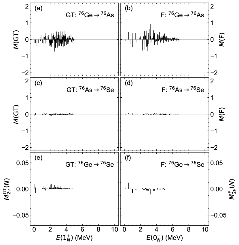
Figure 13: Gamow-Teller and Fermi strength distributions for the single-$\beta$ decays ⁷⁶Ge$\to^{76}$As (a,b) and ⁷⁶As$\to^{76}$Se (c,d), and for the $2\nu\beta\beta$ decay ⁷⁶Ge$\to^{76}$Se (e,f) as functions of the excitation energies of the $N$th intermediate states $1^{+}_{N}$ and $0^{+}_{N}$.

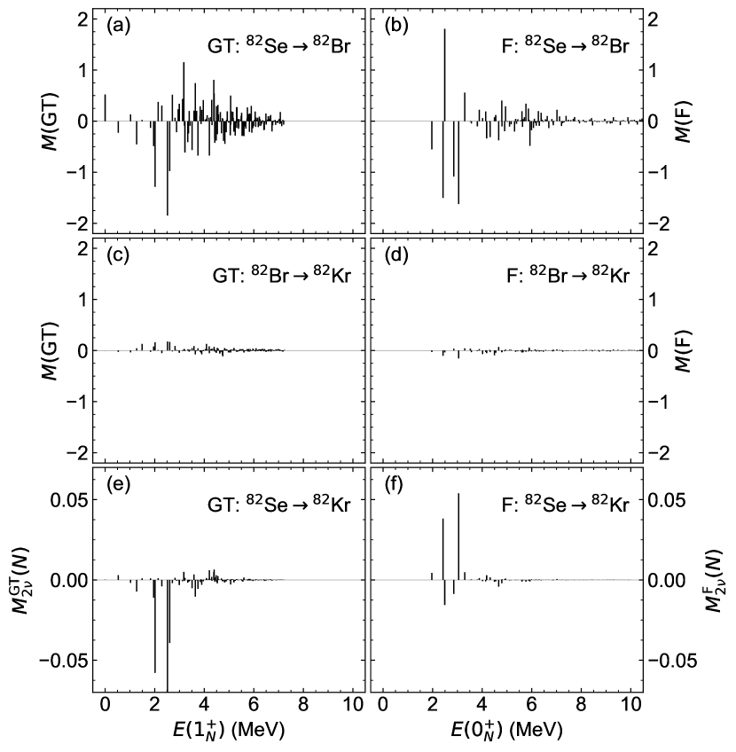
Figure 14: Same as Fig. 13, but for the single-$\beta$ decays ⁸²Se$\to^{82}$Br (a,b) and ⁸²Br$\to^{82}$Kr (c,d), and for the $2\nu\beta\beta$ decay ⁸²Se$\to^{82}$Kr (e,f).

In Fig. 12 the excitation spectra for the ⁷⁶As and ⁸²Br nuclei calculated with the phenomenological SPEs are compared with those calculated self-consistently by the spherical RHB method. It is found that the quality of the IBFFM-2 description does not drastically differ between the two sets of calculations with different SPEs, except perhaps for the energy levels of the $2^{+}_{1}$ and $0^{+}_{2}$ states. The calculated magnetic dipole moment for the ground state $\mu(1^{+}_{1})=0.388\;\mu_{N}$ for the calculation with the self-consistent SPEs (cf. Table 14) compares well with the data ($+0.559\pm 0.005\;\mu_{N}$). In the calculation with the phenomenological SPEs, the value $\mu(5^{+}_{1})=1.157\;\mu_{N}$ is obtained.

Figures 13 and 14 show the GT $M^{\mathrm{GT}}_{2\nu}$ and Fermi $M^{\mathrm{F}}_{2\nu}$ strength distributions for the single-$\beta$ decays between the even-even and odd-odd nuclei, and the contributions of the terms ${M^{\mathrm{GT}}_{2\nu}}(N)$ and $M^{\mathrm{F}}_{2\nu}(N)$ in the $2\nu\beta\beta$ decay NMEs of ⁷⁶Ge and ⁸²Se. Figures 13(a), 13(b), and 6 show that systematics of both the GT and Fermi strengths for the ⁷⁶Ge$\to^{76}$As decay are similar between the two calculations in that they are more or less evenly distributed. For the ⁸²Se$\to^{82}$Br decay, the phenomenological and RHB SPEs also give rise to similar trends, but the contributions from low-lying states to the GT and Fermi strengths are slightly larger in the former than in the latter [Figs. 14(a), 14(b), and 6]. For both the ⁷⁶As and ⁸²Br $\beta^{-}$ decays, the two calculations consistently give negligible GT and Fermi contributions [panels (c) and (d) of Figs. 13 and 14, and Fig. 7]. From panels (e) and (f) of Figs. 13 and 14, one finds that, especially for the ⁸²Se decay, contributions of the low-energy intermediate states in the calculation that employs the phenomenological SPEs are even more significant than in the corresponding results obtained by using the RHB SPEs (cf. Fig. 8).

Table 7: Gamow-Teller $M^{\mathrm{GT}}_{2\nu}$, Fermi $M^{\mathrm{F}}_{2\nu}$, and unquenched total $M_{2\nu}$ (14) NMEs for the $0^{+}_{1}\to 0^{+}_{1}$ and $0^{+}_{1}\to 0^{+}_{2}$ $2\nu\beta\beta$ decays of ⁷⁶Ge and ⁸²Se, obtained with the SPEs computed self-consistently (“DD-PC1”) and those taken from Ref. [78] (“Phen.”). Note that $Q_{\beta\beta,\mathrm{ex}}$ values are used for both calculations.

		76Ge		82Se
		DD-PC1	Phen.	DD-PC1	Phen.
$0^{+}_{1}$	$M^{\mathrm{GT}}_{2\nu}$	$0.034$	$0.069$	$-0.045$	$-0.103$
	$M^{\mathrm{F}}_{2\nu}$	$-0.007$	$-0.022$	0.015	0.037
	$|M_{2\nu}|$	0.062	0.134	0.087	0.203
$0^{+}_{2}$	$M^{\mathrm{GT}}_{2\nu}$	$0.078$	$0.118$	$0.070$	0.073
	$M^{\mathrm{F}}_{2\nu}$	$-0.069$	$-0.101$	$-0.064$	$-0.108$
	$|M_{2\nu}|$	0.194	0.292	0.177	0.225

Table 7 shows the Gamow-Teller $M^{\mathrm{GT}}_{2\nu}$, Fermi $M^{\mathrm{F}}_{2\nu}$, and (unquenched) $2\nu\beta\beta$-decay NMEs $M_{2\nu}$ of the $0^{+}_{1}\to 0^{+}_{1}$ and $0^{+}_{1}\to 0^{+}_{2}$ transitions of ⁷⁶Ge and ⁸²Se, calculated with the phenomenological SPEs of Ref. [78], and with those computed self-consistently within the spherical RHB method. The calculation with the phenomenological SPEs generally gives larger NMEs than with the RHB ones for both ⁷⁶Ge and ⁸²Se. If a typical effective $g_{\mathrm{A}}$ value, $g_{\mathrm{A,eff}}=1$, is used, then the $M_{2\nu}(0^{+}_{1}\to 0^{+}_{1})$ matrix elements for ⁷⁶Ge (⁸²Se) computed with the phenomenological SPEs are reduced to $\approx 0.083$ (0.126), which better agrees with experiment than with the SPEs provided by the RHB method.

V.5.2 Choice of the EDF

Second, NMEs are computed by using the results of the constrained Hartree-Fock-Bogoliubov (HFB) calculations based on the Gogny-D1M [79] EDF. The ¹⁹⁸Pt$\to^{198}$Hg decay is taken as an example, since the derived IBM-2 parameters for the initial and final even-even nuclei, and the SPEs for the odd-odd nucleus ¹⁹⁸Au are available from the previous mapped IBM-2 results [68, 31]. The $\tilde{\epsilon}_{j_{\rho}}$ and $v_{j_{\rho}}^{2}$ values for ¹⁹⁸Au are obtained in the same manner as described in the previous section. The SPEs obtained from the Gogny-D1M HFB calculation, as well as the $\tilde{\epsilon}_{j_{\rho}}$ and $v_{j_{\rho}}^{2}$ values computed within the BCS approximation, are found in Table 8. The strength parameters for $\hat{V}_{\mathrm{BF}}^{\rho}$, available from Ref. [31], are used here for the IBFFM-2 Hamiltonian without modification, but only the parameters for the residual neutron-proton interaction $\hat{V}_{\nu\pi}$ are changed as $v_{\mathrm{d}}=-0.30\to-0.08$ MeV, $v_{\mathrm{ssd}}=-0.033\to 0$ MeV, and $v_{\mathrm{t}}=0\to 0.1$ MeV.

The IBM-2 energy spectra for the ¹⁹⁸Pt and ¹⁹⁸Hg computed with the microscopic input from the Gogny-D1M HFB calculation are found in Figs. 4 and 5 of Ref. [68], and in Fig. 2 of Ref. [31], respectively, which can be compared with the present results shown in Fig. 3. The description of the low-energy spectra of the even-even nuclei appears to be qualitatively similar between the calculations with the Gogny-D1M and DD-PC1 EDFs. In addition, the calculated energy spectra of the low-lying positive-parity states of the intermediate nucleus ¹⁹⁸Au from the DD-PC1 and D1M EDFs are compared with each other in Fig. 15. The description of the observed spectrum appears to be better when the DD-PC1 functional is used than for the D1M one. As for the magnetic dipole moment for the ground state $\mu(5^{+}_{1})$, however, the IBFFM-2 with the D1M EDF reproduces correctly the experimental value [80], while the calculation with the DD-PC1 EDF does not (cf. Appendix E).

Figure 15: Energy spectra for the low-lying positive-parity states of ¹⁹⁸Au computed by the IBFFM-2 based on the DD-PC1 and Gogny-D1M EDFs. The corresponding experimental spectrum is also shown for comparison.

Table 8 compares the predicted $M^{\mathrm{GT}}_{2\nu}$, $M^{\mathrm{F}}_{2\nu}$, and total (unquenched) $M_{2\nu}$ matrix elements for the $0^{+}_{1}\to 0^{+}_{1}$ and $0^{+}_{1}\to 0^{+}_{2}$ decays of ¹⁹⁸Pt, that are obtained with the relativistic DD-PC1 and nonrelativistic Gogny-D1M EDFs. In both cases, the theoretical $Q_{\beta\beta}$ values, $Q_{\beta\beta,\mathrm{th}}$, are used. For the Gogny-D1M EDF, the $Q_{\beta\beta,\mathrm{th}}$ value of $Q_{\beta\beta,\mathrm{th}}=0.667$ MeV is obtained, which is about half the value for the DD-PC1 EDF, $Q_{\beta\beta,\mathrm{th}}=1.290$ MeV. As shown in Table 8, for both the $0^{+}_{1}\to 0^{+}_{1}$ and $0^{+}_{1}\to 0^{+}_{2}$ transitions, the calculation with the Gogny-D1M EDF produces $M_{2\nu}$ that is by more than a factor of 4 to 5 larger than the one with the DD-PC1 EDF. The discrepancy in the prediction of NME appears to be, to some extent, due to the difference between the SPEs provided by the two functionals. For instance, the energy splitting between the lowest neutron orbital $1h_{9/2}$ and the second lowest orbital $2f_{7/2}$ is $\Delta{\epsilon}=\epsilon_{2f_{7/2}}-\epsilon_{1h_{9/2}}\approx 0.5$ MeV for the Gogny D1M, while the energy gap is much larger for the DD-PC1, $\Delta\epsilon\approx 2.5$ MeV [see Table 15 in Appendix B]. It should be nevertheless kept in mind that several other model assumptions are made in each step of the theoretical procedure. To identify the major cause of the discrepancy between the results from different functionals, a more systematic investigation may be in order.

Table 8: Comparison of Gamow-Teller $M^{\mathrm{GT}}_{2\nu}$, Fermi $M^{\mathrm{F}}_{2\nu}$, and unquenched total $M_{2\nu}$ NMEs for the $0^{+}_{1}\to 0^{+}_{1}$ and $0^{+}_{1}\to 0^{+}_{2}$ $2\nu\beta\beta$ decays of ¹⁹⁸Pt, calculated with the DD-PC1 and Gogny-D1M EDFs. $Q_{\beta\beta,\mathrm{th}}=1.2895$ MeV and $Q_{\beta\beta,\mathrm{th}}=0.6672$ MeV are used for the DD-PC1 and Gogny-D1M EDFs, respectively.

EDF	$0^{+}_{1}$			$0^{+}_{2}$
	$M^{\mathrm{GT}}_{2\nu}$	$M^{\mathrm{F}}_{2\nu}$	$|M_{2\nu}|$	$M^{\mathrm{GT}}_{2\nu}$	$M^{\mathrm{F}}_{2\nu}$	$|M_{2\nu}|$
DD-PC1	$-0.016$	$0.001$	0.026	$-0.008$	$-0.000$	0.012
D1M	$-0.074$	$0.000$	0.120	$-0.034$	$-0.000$	0.054

V.5.3 Truncation of the intermediate state energy

Throughout this study, the fixed energy cutoff $E_{x}=10$ MeV is considered for the intermediate $1^{+}$ and $0^{+}$ states of the odd-odd nuclei included in the $2\nu\beta\beta$-decay NMEs. In most cases, both the $M^{\mathrm{GT}}_{2\nu}$ and $M^{\mathrm{F}}_{2\nu}$ matrix elements saturate, if the energy cutoff is made at $E_{x}\gtrsim 6$ MeV.

An exception is perhaps the ⁴⁸Ca decay, since as shown in Figs. 6, 7, and 8, there are sizable contributions to the GT and Fermi strengths from those states with $E_{x}\gtrsim 5$ MeV. The present IBFFM-2 calculation yields 75 $1^{+}$ and 30 $0^{+}$ states below $E_{x}=10$ MeV in the intermediate nucleus ⁴⁸Sc, but there are also more states at $E_{x}>10$ MeV. If the truncation is set to $E_{x}=20$ MeV, for instance, the resultant $M^{\mathrm{GT}}_{2\nu}$ and $M^{\mathrm{F}}_{2\nu}$ values turn out to be by $\approx 20\,\%$ smaller than those with $E_{x}=10$ MeV.

In the previous IBFFM-2 calculation by Yoshida and Iachello [21] for the $2\nu\beta\beta$ decays of ¹²⁸Te and ¹³⁰Te, the truncation was set to be a much lower energy, $E_{x}=3$ MeV. If the same energy cutoff $E_{x}=3$ MeV is applied to the present calculation for the ¹³⁰Te decay, then the GT matrix element $|M^{\mathrm{GT}}_{2\nu}|$, for instance, is reduced by a factor of 3. While the calculation in Ref. [21] obtained 100 $1^{+}$ and 50 $0^{+}$ states below $E_{x}=3$ MeV, here only 20 $1^{+}$ and 6 $0^{+}$ states are found in the same energy range. Furthermore, the GT part of the $2\nu\beta\beta$ decay NME was shown [21] to be accounted for almost solely by the lowest $1^{+}$ intermediate state. On the other hand, the corresponding GT strength is here more evenly distributed up to $E_{x}=8$ MeV (see Fig. 8). These differences between the two calculations seem to have originated from the different starting points to determine the IBM-2 and IBFFM-2 Hamiltonians. In Ref. [21], these ingredients are more or less taken from the empirical data, whereas the present calculation is largely based on the nuclear EDF.

VI Concluding remarks

The $2\nu\beta\beta$ decay has been investigated within the IBM-2 and IBFFM-2 that are based on the nuclear density functional theory. By mapping the quadrupole triaxial deformation energy surface, computed by the constrained RHB method that employs the universal functional DD-PC1 and the separable pairing interaction, onto the corresponding bosonic energy surface, the IBM-2 Hamiltonian for the even-even initial- and final-state nuclei of the considered $\beta\beta$ decays have been determined. The same EDF calculation has provided the essential ingredients of the IBFFM-2 for describing the intermediate odd-odd nuclei and the GT and Fermi transition operators.

The EDF-based IBM-2 and IBFFM-2 give reasonable descriptions of the excitation spectra and electromagnetic transition rates for the low-lying states of the relevant even-even and odd-odd nuclei. The GT and Fermi parts of the $2\nu\beta\beta$ decays are, in most cases, predicted to be dominated by the contributions from the low-lying intermediate states, the illustrative examples being the ¹⁰⁰Mo$\to^{100}$Ru, ¹¹⁶Cd$\to^{116}$Sn, ¹²⁸Te$\to^{128}$Xe, and ¹⁵⁰Nd$\to^{150}$Sm decays. Two different parametrizations for the effective values of the axial vector coupling constants $g_{\mathrm{A}}$ for $2\nu\beta\beta$ decay have been introduced: one that is modest, decreasing gradually from $g_{\mathrm{A,eff}}\approx 0.7$ to 0.5, and the other varying more drastically from $g_{\mathrm{A,eff}}\approx 0.9$ to 0.3 as functions of the mass number $A$. The resultant $2\nu\beta\beta$-decay NMEs, with these $g_{\mathrm{A,eff}}$ factors taken into account, exhibit a similar trend with $A$ to the observed ones. As shown in Fig. 11, the previous theoretical predictions on the NMEs are quite at variance with each other. For most of the $2\nu\beta\beta$-decay candidates, the present values of the NMEs more or less fall into the range of various other theoretical values. However, as compared to the experiment and majority of the earlier theoretical calculations, the present calculations have given particularly small NMEs for the ⁷⁶Ge and ⁸²Se $0^{+}_{1}\to 0^{+}_{1}$ decays even without the quenching. The prediction of the NMEs is shown to be rather sensitive to the spherical SPEs for the odd particles, and to the choice of the underlying EDF.

This paper presents a way of calculating simultaneously the low-lying states of the relevant even-even and odd-odd nuclei, and the $\beta$ and $\beta\beta$ decay NMEs, based largely on the nuclear EDF. Within this theoretical scheme, one can go further to explore the $0\nu\beta\beta$ decay. At the same time, it remains an open problem to identify major sources of uncertainties in the prediction of the NMEs within the employed theoretical scheme, whether it is the SPEs, the use of the specific form of the IBM-2 or IBFFM-2 Hamiltonian, the deficiency of the underlying EDF, or some combinations of these. As an instance, correlations between the choice of the EDF as a microscopic input and the form of the Hamiltonian or building blocks of the IBM-2 would be among the most relevant factors that significantly affect the quality of the wave functions for the initial and final states of a given decay process. While the current study has resorted to a particular type of the nuclear EDF and pairing interaction, in some cases there appear notable differences between the topology of the triaxial quadrupole potential energy surface obtained from different classes of the EDF, such as the ones in the relativistic and nonrelativistic regimes. The present form of the IBM-2 Hamiltonian does not account for some important features of the SCMF energy surfaces, including the triaxial minimum or competing mean-field minima, and a more reliable prediction of the initial- and final-state wave functions would require the inclusions of some higher-order boson terms in the Hamiltonian or the configuration mixing between normal and intruder states. The configuration mixing would be of particular importance for an accurate description of the excited $0^{+}$ states. By comparing the low-energy spectra and electromagnetic transition rates resulting from different versions of the IBM-2 calculations with different microscopic inputs, one could quantify which of these extensions or terms of the Hamiltonian are most relevant to change the spectroscopic predictions and the final results for the NMEs. These problems will be taken up and investigated in a more systematic manner elsewhere.

Appendix A Parameters for the IBM-2 Hamiltonian

Table 9: Derived strength parameters for the IBM-2 Hamiltonian $\hat{H}_{\mathrm{B}}$ for even-even nuclei.

Nucleus	$\epsilon$	$-\kappa$	$-\kappa_{\nu}$	$-\kappa_{\pi}$	$\chi_{\nu}$	$\chi_{\pi}$	$\kappa^{\prime}$
	(MeV)	(MeV)	(keV)	(keV)			(keV)
46Ca	1.50		$57$		$-1.30$
48Ca	1.50		$57$
48Ti	1.25	$0.59$			$-1.10$	$-1.10$
76Ge	0.60	0.38			$-$0.90	$-$0.50
76Se	0.84	0.22			0.90	0.50	21
82Se	0.80	0.70			$-$1.00	$-$1.00
82Kr	1.16	0.35			$-$0.40	$-$0.40
96Zr	0.80	0.35			$-$0.45	0.47	21
96Mo	0.69	0.44			$-$0.65	0.45	9.5
100Mo	0.58	0.35			$-$0.50	0.45
100Ru	0.50	0.44			$-$0.70	$-0.40$
110Pd	0.56	0.29			$-$0.30	0.47
110Cd	0.40	0.51			$-$1.10	$-$0.45	55
116Sn	1.50		$57$		0.80
116Cd	0.85	0.23			$-0.30$	0.40
118Sn	1.50		$57$		0.80
124Sn	1.50		$57$		0.80
124Te	0.51	0.48			0.44	$-$0.13
128Te	0.78	0.48			0.40	$-$0.90
128Xe	0.42	0.42			0.40	$-$0.80
130Te	0.95	0.48			0.30	$-$0.78
130Xe	0.56	0.44			0.25	$-$0.86
136Xe	1.50			$57$		$-0.80$
136Ba	1.06	0.34			$-0.28$	$-0.95$
148Nd	0.43	0.27			$-$0.78	$-$0.54
150Nd	0.21	0.24			$-$0.80	$-$0.50	$-$8
150Sm	0.10	0.21			$-$0.70	$-$0.55	9.5
198Pt	0.26	0.32			0.25	0.45
198Hg	0.60	0.47			1.00	0.90
200Hg	0.55	0.41			1.20	1.00

Table 9 lists the adopted IBM-2 parameters for the relevant even-even nuclei, determined based on the SCMF calculations. It is noted that the nuclei ⁴⁶Ca, ¹¹⁸Sn, ¹⁴⁸Nd, and ²⁰⁰Hg are not involved in the studied $\beta\beta$ decays, but are here considered only as the boson cores for the IBFFM-2 calculations (see compositions of the odd-odd nuclei in Table 1). The calculated low-energy spectra of these nuclei are in a good agreement with the experimental data to the same extent as those shown in Fig. 3. Note also that, for majority of the studied even-even nuclei, the $\hat{L}\cdot\hat{L}$ term does not play a major role, and is considered only in a few nuclei that exhibit a relatively large deformation ($\beta\gtrsim 0.15$) in the energy surface, such as ⁷⁶Se and ¹⁵⁰Nd (see Fig. 1). For the semi-magic nuclei ^46,48Ca, ^116,118,124Sn, and ¹³⁶Xe, the SCMF energy surface shows only spherical minimum, which makes it difficult to uniquely determine the Hamiltonian parameters. In these cases, therefore, common values $\epsilon_{d}=1.5$ MeV and $\kappa_{\rho}=-0.057$ MeV are used.

Appendix B Single-particle energies and occupation probabilities for the IBFFM-2

Table 10: Neutron and proton spherical single-particle energies $\epsilon_{j_{\rho}}$ (in MeV) and occupation probabilities $v^{2}_{j_{\rho}}$ obtained from the spherical RHB calculations for the odd-odd nuclei ⁴⁸Sc, ⁷⁶As, and ⁸²Br.

Nucleus		Neutron orbital					Proton orbital
		$2p_{1/2}$	$2p_{3/2}$	$1f_{5/2}$	$1f_{7/2}$	$1g_{9/2}$	$2p_{1/2}$	$2p_{3/2}$	$1f_{5/2}$	$1f_{7/2}$	$1g_{9/2}$
48Sc	$\epsilon_{j_{\rho}}$	$-3.239$	$-5.163$	$-2.233$	$-10.381$		$1.253$	$-0.759$	$0.726$	$-7.785$
	$v^{2}_{j_{\rho}}$	$0.005$	$0.011$	$0.007$	$0.865$		$0.001$	$0.002$	$0.004$	$0.129$
76As	$\epsilon_{j_{\rho}}$	$-12.071$	$-14.145$	$-14.097$		$-7.950$	$-6.422$	$-8.203$	$-8.570$		$-2.729$
	$v^{2}_{j_{\rho}}$	$0.966$	$0.985$	$0.982$		$0.316$	$0.116$	$0.411$	$0.515$		$0.017$
82Br	$\epsilon_{j_{\rho}}$	$-13.480$	$-15.487$	$-16.010$		$-9.534$	$-7.839$	$-9.462$	$-10.739$		$-4.747$
	$v^{2}_{j_{\rho}}$	$0.980$	$0.990$	$0.990$		$0.704$	$0.137$	$0.462$	$0.793$		$0.019$

Table 11: Same as Table 10, but for the ⁹⁶Nb, ¹⁰⁰Tc, ¹¹⁰Ag, and ¹¹⁶In nuclei.

Nucleus		Neutron orbital					Proton orbital
		$3s_{1/2}$	$2d_{3/2}$	$2d_{5/2}$	$1g_{7/2}$	$1h_{11/2}$	$2p_{1/2}$	$2p_{3/2}$	$1f_{5/2}$	$1g_{7/2}$	$1g_{9/2}$
96Nb	$\epsilon_{j_{\rho}}$	$-4.655$	$-4.249$	$-6.596$	$-5.645$	$-1.380$	$-9.685$	$-11.406$	$-13.164$	$0.582$	$-7.167$
	$v^{2}_{j_{\rho}}$	$0.073$	$0.068$	$0.474$	$0.211$	$0.014$	$0.864$	$0.962$	$0.981$	$0.004$	$0.150$
100Tc	$\epsilon_{j_{\rho}}$	$-5.479$	$-5.182$	$-7.489$	$-6.955$	$-2.605$	$-10.117$	$-11.839$	$-13.716$	$-0.064$	$-7.600$
	$v^{2}_{j_{\rho}}$	$0.095$	$0.092$	$0.544$	$0.381$	$0.022$	$0.909$	$0.967$	$0.980$	$0.008$	$0.336$
110Ag	$\epsilon_{j_{\rho}}$	$-7.205$	$-7.081$	$-9.274$	$-9.654$	$-5.147$	$-11.703$	$-13.384$	$-15.563$	$-2.169$	$-9.236$
	$v^{2}_{j_{\rho}}$	$0.192$	$0.184$	$0.784$	$0.841$	$0.040$	$0.963$	$0.983$	$0.989$	$0.010$	$0.710$
116In	$\epsilon_{j_{\rho}}$	$-7.912$	$-7.964$	$-10.143$	$-10.959$	$-6.368$	$-12.798$	$-14.497$	$-16.617$	$-3.362$	$-10.239$
	$v^{2}_{j_{\rho}}$	$0.437$	$0.456$	$0.911$	$0.948$	$0.102$	$0.988$	$0.994$	$0.996$	$0.005$	$0.901$

Table 12: Same as Table 10, but for the ¹²⁴Sb, ¹²⁸I, ¹³⁰I, and ¹³⁶Cs nuclei.

Nucleus		Neutron orbital					Proton orbital
		$3s_{1/2}$	$2d_{3/2}$	$2d_{5/2}$	$1g_{7/2}$	$1h_{11/2}$	$3s_{1/2}$	$2d_{3/2}$	$2d_{5/2}$	$1g_{7/2}$	$1h_{11/2}$
124Sb	$\epsilon_{j_{\rho}}$	$-8.718$	$-8.987$	$-11.180$	$-12.478$	$-7.658$	$-1.197$	$-1.957$	$-4.110$	$-5.526$	$-1.108$
	$v^{2}_{j_{\rho}}$	$0.735$	$0.785$	$0.954$	$0.972$	$0.398$	$0.002$	$0.004$	$0.015$	$0.114$	$0.004$
128I	$\epsilon_{j_{\rho}}$	$-9.362$	$-9.734$	$-11.949$	$-13.646$	$-8.606$	$-1.434$	$-2.193$	$-4.332$	$-6.087$	$-1.496$
	$v^{2}_{j_{\rho}}$	$0.763$	$0.826$	$0.961$	$0.979$	$0.537$	$0.006$	$0.012$	$0.039$	$0.339$	$0.011$
130I	$\epsilon_{j_{\rho}}$	$-9.449$	$-9.860$	$-12.088$	$-13.845$	$-8.737$	$-2.038$	$-2.834$	$-4.954$	$-6.889$	$-2.246$
	$v^{2}_{j_{\rho}}$	$0.841$	$0.885$	$0.973$	$0.984$	$0.662$	$0.005$	$0.010$	$0.033$	$0.345$	$0.010$
136Cs	$\epsilon_{j_{\rho}}$	$-10.141$	$-10.690$	$-12.865$	$-15.120$	$-9.820$	$-2.819$	$-3.676$	$-5.685$	$-8.113$	$-3.377$
	$v^{2}_{j_{\rho}}$	$0.959$	$0.975$	$0.994$	$0.997$	$0.933$	$0.006$	$0.013$	$0.039$	$0.583$	$0.014$

Table 13: Same as Table 10, but for the ¹⁵⁰Pm, and ¹⁹⁸Au nuclei.

Nucleus		Neutron orbital						Proton orbital
		$3p_{1/2}$	$3p_{3/2}$	$2f_{5/2}$	$2f_{7/2}$	$1h_{9/2}$	$1i_{13/2}$	$3s_{1/2}$	$2d_{3/2}$	$2d_{5/2}$	$1g_{7/2}$	$1h_{9/2}$	$1h_{11/2}$
150Pm	$\epsilon_{j_{\rho}}$	$-1.413$	$-2.045$	$-2.452$	$-4.585$	$-5.491$	$-2.043$	$-3.965$	$-4.782$	$-6.625$	$-9.778$	$2.366$	$-4.946$
	$v^{2}_{j_{\rho}}$	$0.012$	$0.016$	$0.033$	$0.186$	$0.499$	$0.027$	$0.030$	$0.072$	$0.376$	$0.958$	$0.004$	$0.063$
198Au	$\epsilon_{j_{\rho}}$	$-7.037$	$-7.405$	$-8.424$	$-10.687$	$-13.191$	$-8.954$	$-6.853$	$-8.421$	$-9.902$	$-14.382$	$-3.198$	$-9.213$
	$v^{2}_{j_{\rho}}$	$0.264$	$0.391$	$0.779$	$0.968$	$0.990$	$0.887$	$0.250$	$0.832$	$0.961$	$0.995$	$0.010$	$0.942$

Tables 10, 11, 12, and 13 show the employed neutron and proton spherical SPEs $\epsilon_{j_{\rho}}$ and occupation probabilities $v^{2}_{j_{\rho}}$ within the considered fermion configuration spaces for the intermediate odd-odd nuclei. They are obtained by the spherical RHB calculation with the DD-PC1 EDF constrained to zero deformation (see Ref. [30] for details). As seen in Table 10, only the configuration space for ⁴⁸Sc includes the $1f_{7/2}$ orbital for both proton and neutron, since in this case the ⁴⁰Ca nucleus is taken as the boson core, and the low-lying states of ⁴⁸Sc are assumed to be mainly composed of the proton and neutron $1f_{7/2}$ single-particle configurations. As seen in Table 11, the proton $1g_{7/2}$ orbital, which belongs to the next major shell $Z=50-82$, is included in the calculation. This gives rise to a non-vanishing contribution to the Fermi matrix element by the coupling between the neutron and proton $1g_{7/2}$ orbitals. The $\pi 1g_{7/2}$ orbital is included in order to see to what extent the Fermi transition, arising in that way, contributes to the final result on the $M_{2\nu}$ matrix element. For the same reason, the proton single-particle spaces for ¹⁵⁰Pm and ¹⁹⁸Au include the $1h_{9/2}$ orbital, which basically comes from the next major oscillator shell $82<Z<126$.

Table 14: Phenomenological single-particle energies $\epsilon_{j_{\rho}}$ (in MeV) that are taken from Ref. [78] (denoted by “Phen.”), and the quasiparticle energies $\tilde{\epsilon}_{j_{\rho}}$ (in MeV) and occupation probabilities $v^{2}_{j_{\rho}}$ obtained from the BCS calculation for ⁷⁶As and ⁸²Br. The corresponding quantities computed self-consistently by the spherical RHB method are also shown for comparison. See the main text in Sec. V.5.1.

Nucleus			Neutron orbital				Proton orbital
			$2p_{1/2}$	$2p_{3/2}$	$1f_{5/2}$	$1g_{9/2}$	$2p_{1/2}$	$2p_{3/2}$	$1f_{5/2}$	$1g_{9/2}$
76As	$\epsilon_{j_{\rho}}$	Phen.	$-7.839$	$-9.828$	$-8.709$	$-6.262$	$-7.839$	$-9.828$	$-8.709$	$-6.262$
		RHB	$-12.071$	$-14.145$	$-14.097$	$-7.950$	$-6.422$	$-8.203$	$-8.570$	$-2.729$
	$\tilde{\epsilon}_{j_{\rho}}$	Phen.	$1.880$	$3.548$	$2.554$	$1.408$	$2.063$	$1.449$	$1.529$	$3.404$
		RHB	$3.570$	$5.251$	$5.813$	$1.456$	$2.671$	$1.739$	$1.792$	$5.896$
	$v^{2}_{j_{\rho}}$	Phen.	$0.841$	$0.961$	$0.921$	$0.395$	$0.128$	$0.656$	$0.282$	$0.043$
		RHB	$0.966$	$0.985$	$0.982$	$0.316$	$0.116$	$0.411$	$0.515$	$0.017$
82Br	$\epsilon_{j_{\rho}}$	Phen.	$-7.839$	$-9.828$	$-8.709$	$-6.262$	$-7.839$	$-9.828$	$-8.709$	$-6.262$
		RHB	$-13.480$	$-15.487$	$-16.010$	$-9.534$	$-7.839$	$-9.462$	$-10.739$	$-4.747$
	$\tilde{\epsilon}_{j_{\rho}}$	Phen.	$2.673$	$4.510$	$3.456$	$1.520$	$1.637$	$1.677$	$1.328$	$2.863$
		RHB	$4.310$	$5.900$	$7.184$	$1.394$	$2.368$	$1.633$	$1.963$	$4.974$
	$v^{2}_{j_{\rho}}$	Phen.	$0.934$	$0.978$	$0.962$	$0.745$	$0.207$	$0.807$	$0.466$	$0.057$
		RHB	$0.980$	$0.990$	$0.990$	$0.704$	$0.137$	$0.462$	$0.793$	$0.019$

Table 15: Single-particle $\epsilon_{j_{\rho}}$ and quasiparticle $\tilde{\epsilon}_{j_{\rho}}$ energies (both in MeV), and occupation probabilities $v^{2}_{j_{\rho}}$ employed for the IBFFM-2 calculations based on the Gogny-D1M and DD-PC1 EDFs. The $\tilde{\epsilon}_{j_{\rho}}$ and $v^{2}_{j_{\rho}}$ values for the Gogny-D1M EDF are obtained from the BCS calculation. See the main text in Sec. V.5.2.

		Neutron orbital						Proton orbital
		$3p_{1/2}$	$3p_{3/2}$	$2f_{5/2}$	$2f_{7/2}$	$1h_{9/2}$	$1i_{13/2}$	$3s_{1/2}$	$2d_{3/2}$	$2d_{5/2}$	$1g_{7/2}$	$1h_{9/2}$	$1h_{11/2}$
$\epsilon_{j_{\rho}}$	D1M	$-7.285$	$-8.234$	$-8.344$	$-11.147$	$-11.690$	$-8.855$	$-7.738$	$-8.615$	$-10.313$	$-12.882$	$-2.505$	$-8.565$
	DD-PC1	$-7.037$	$-7.405$	$-8.424$	$-10.687$	$-13.191$	$-8.954$	$-6.853$	$-8.421$	$-9.902$	$-14.382$	$-3.198$	$-9.213$
$\tilde{\epsilon}_{j_{\rho}}$	D1M	$1.090$	$0.895$	$0.934$	$3.295$	$3.823$	$1.234$	$0.861$	$1.313$	$2.828$	$5.335$	$5.182$	$1.275$
	DD-PC1	$1.301$	$1.161$	$1.352$	$3.166$	$5.632$	$1.668$	$1.329$	$1.333$	$2.559$	$6.912$	$4.375$	$1.899$
$v^{2}_{j_{\rho}}$	D1M	$0.189$	$0.651$	$0.704$	$0.983$	$0.987$	$0.861$	$0.570$	$0.880$	$0.977$	$0.994$	$0.007$	$0.872$
	DD-PC1	$0.264$	$0.391$	$0.779$	$0.968$	$0.990$	$0.887$	$0.250$	$0.832$	$0.961$	$0.995$	$0.010$	$0.942$

Table 14 lists the phenomenological SPEs $\epsilon_{j_{\rho}}$ of Ref. [78], and the quasiparticle energies $\tilde{\epsilon}_{j_{\rho}}$ and occupation probabilities $v^{2}_{j_{\rho}}$ for ⁷⁶As and ⁸²Se calculated within the BCS approximation, in comparison to the RHB results. Table 15 summarizes the $\epsilon_{j_{\rho}}$, $\tilde{\epsilon}_{j_{\rho}}$, and $v^{2}_{j_{\rho}}$ for ¹⁹⁸Au, obtained with the RHB method with the DD-PC1 EDF, and those based on the HFB calculation using the Gogny-D1M EDF.

Appendix C Parameters for the IBFFM-2 Hamiltonian

Table 16: Adopted IBFFM-2 parameters for the boson-fermion interactions $\hat{V}_{\mathrm{BF}}^{\rho}$ (6)–(II.3), and for the residual neutron-proton interaction $\hat{V}_{\nu\pi}$ (II.3), for the intermediate odd-odd nuclei. For each odd-odd nucleus, the values of the strength parameters $\Gamma_{\rho}$, $\Lambda_{\rho}$, and $A_{\rho}$ (with $\rho=\nu$ and $\pi$) that appear in the upper and lower rows refer to the ones employed for computing the positive- and negative-parity states of the neighboring odd-mass nuclei, respectively. All the parameters are in MeV units.

Nucleus	$\Gamma_{\nu}$	$\Lambda_{\nu}$	$A_{\nu}$	$\Gamma_{\pi}$	$\Lambda_{\pi}$	$A_{\pi}$	$v_{\mathrm{d}}$	$v_{\mathrm{ssd}}$	$v_{\mathrm{t}}$
48Sc							0.6
	0.3	1.0		0.3
76As	0.3	2.0		1.0			0.8		0.02
	0.3	7.5	$-0.6$	0.3	1.6	$-0.8$
82Br	0.3	2.1		2.5				$-0.4$
	0.3	0.8		0.3	0.8
96Nb	0.3	0.4		0.3	0.9	$-0.5$	0.8
	0.3		$-1.5$	0.3	1.6	$-0.3$
100Tc	0.3	0.35		0.3	0.9		$-0.08$		0.05
	0.3			0.3	5.0	$-1.0$
110Ag	0.3	2.8		0.3	8.0		$-0.08$		0.8
	0.3			0.3	1.4
116In	0.3	0.2	$-0.15$	0.3			$-0.8$		0.4
	0.3	0.2	$-0.15$	1.0
124Sb	0.3	10.0	$-1.0$	1.2			$-0.03$		0.135
	0.3	2.0	$-0.60$	1.2
128I	0.3	6.5		0.3	0.6	$-1.0$		$-0.51$
	0.3	0.9	$-0.2$	0.3		$-1.05$
130I	0.3	7.6		0.3	0.8	$-0.75$	$-0.08$		0.01
	0.3	0.9	$-0.5$	0.3		$-1.05$
136Cs	0.6			0.6	0.2	$-0.9$	$-0.08$		0.09
	0.6			0.6	0.2	$-0.9$
150Pm	0.3	10.0	$-0.8$	0.3	0.4	$-1.0$	$-0.08$		0.14
	0.3	0.6	$-1.0$	3.0
198Au	0.3	1.6		0.3	0.6		$-0.08$		0.05
	0.3	1.6	$-0.4$	0.3	0.6

Table 16 lists the adopted strength parameters for the boson-fermion interaction $\hat{V}_{\mathrm{BF}}^{\rho}$ (6)–(II.3) and the residual neutron-proton interaction $\hat{V}_{\nu\pi}$ (II.3) in the IBFFM-2 Hamiltonian. For many of the odd-odd nuclei, the strength parameters for the dynamical terms are assumed to take a fixed value $\Gamma_{\rho}=0.3$ MeV. In most cases, only the delta and tensor terms are considered. The parameters for $\hat{V}_{\nu\pi}$ also do not differ too much from one nucleus to another within the same mass region. For instance, the parameter $v_{\mathrm{d}}$ is stable in the mass $A\gtrsim 100$ region, except for ¹¹⁶In.

Appendix D Coefficients for one-particle transfer operators

The present formulation of the one-particle transfer operators is based on the one developed in the earlier IBFM-2 studies for the single-$\beta$ decays of mass $A\approx 130$ nuclei [81, 82]. Within the generalized seniority considerations, the coefficients $\zeta_{j}$, $\zeta_{jj^{\prime}}$, $\theta_{j}$, and $\theta_{jj^{\prime}}$ in Eqs. (21a) and (21b) are assumed to take the forms

$$\zeta_{j_{\rho}} =u_{j_{\rho}}\frac{1}{K_{j_{\rho}}^{\prime}},$$ (32a)

$$\zeta_{j_{\rho}j_{\rho}^{\prime}} =-v_{j_{\rho}}\beta_{j_{\rho}^{\prime}j_{\rho}}\sqrt{\frac{10}{N_{\rho}(2j_{\rho}+1)}}\frac{1}{KK_{j_{\rho}}^{\prime}},$$ (32b)

$$\theta_{j_{\rho}} =\frac{v_{j_{\rho}}}{\sqrt{N_{\rho}}}\frac{1}{K_{j_{\rho}}^{\prime\prime}},$$ (32c)

$$\theta_{j_{\rho}j_{\rho}^{\prime}} =u_{j_{\rho}}\beta_{j_{\rho}^{\prime}j_{\rho}}\sqrt{\frac{10}{2j_{\rho}+1}}\frac{1}{KK_{j_{\rho}}^{\prime\prime}}.$$ (32d)

The occupation $v_{j_{\rho}}$ and unoccupation $u_{j_{\rho}}$ amplitudes are here provided by the spherical RHB calculation. The factors $K$, $K^{\prime}_{j_{\rho}}$, and $K^{\prime\prime}_{j_{\rho}}$ are given by

$$K=\left(\sum_{j_{\rho}j_{\rho}^{\prime}}\beta_{j_{\rho}j_{\rho}^{\prime}}^{2}\right)^{1/2},$$ (33a)

$$K_{j_{\rho}}^{\prime}=\left[1+2\left(\frac{v_{j_{\rho}}}{u_{j_{\rho}}}\right)^{2}\frac{\braket{(\hat{n}_{s_{\rho}}+1)\hat{n}_{d_{\rho}}}_{0^{+}_{1}}}{N_{\rho}(2j_{\rho}+1)}\frac{\sum_{j_{\rho}^{\prime}}\beta_{j_{\rho}^{\prime}j_{\rho}}^{2}}{K^{2}}\right]^{1/2},$$ (33b)

$$K_{j_{\rho}}^{\prime\prime}=\left[\frac{\braket{\hat{n}_{s_{\rho}}}_{0^{+}_{1}}}{N_{\rho}}+2\left(\frac{u_{j_{\rho}}}{v_{j_{\rho}}}\right)^{2}\frac{\braket{\hat{n}_{d_{\rho}}}_{0^{+}_{1}}}{2j_{\rho}+1}\frac{\sum_{j_{\rho}^{\prime}}\beta_{j_{\rho}^{\prime}j_{\rho}}^{2}}{K^{2}}\right]^{1/2},$$ (33c)

where $\hat{n}_{s_{\rho}}$ is the number operator for the $s_{\rho}$ boson and $\braket{\cdots}_{0^{+}_{1}}$ represents the expectation value of a given operator in the $0^{+}_{1}$ ground state of the even-even nucleus. A more detailed account on the $\beta$-decay operators within the IBFM-2 framework is found in Refs. [81, 82, 29].

Appendix E Electromagnetic properties of the even-even and odd-odd nuclei

The $E2$ operator $\hat{T}^{(E2)}$ in the IBFFM-2 takes the form [29]:

$$\hat{T}^{(E2)}=\hat{T}^{(E2)}_{\mathrm{B}}+\hat{T}^{(E2)}_{\mathrm{F}},$$ (34)

where the first and second terms are the boson and fermion parts, given respectively as

$$\hat{T}^{(E2)}_{\mathrm{B}}=e_{\nu}^{\mathrm{B}}\hat{Q}_{\nu}+e_{\pi}^{\mathrm{B}}\hat{Q}_{\pi}$$ (35)

and

$$\hat{T}^{(E2)}_{\mathrm{F}}=-\frac{1}{\sqrt{5}} \sum_{\rho=\nu,\pi}\sum_{j_{\rho}j_{\rho}^{\prime}}(u_{j_{\rho}}u_{j_{\rho}^{\prime}}-v_{j_{\rho}}v_{j_{\rho}^{\prime}})$$

$$\times\left\langle\ell_{\rho}\frac{1}{2}j_{\rho}\bigg{\|}e^{\mathrm{F}}_{\rho}r^{2}Y^{(2)}\bigg{\|}\ell_{\rho}^{\prime}\frac{1}{2}j_{\rho}^{\prime}\right\rangle(a_{j_{\rho}}^{\dagger}\times\tilde{a}_{j_{\rho}^{\prime}})^{(2)}.$$ (36)

The boson effective charges $e^{\mathrm{B}}_{\nu}=e^{\mathrm{B}}_{\pi}$ are adjusted to reproduce the experimental $B(E2;2^{+}_{1}\rightarrow 0^{+}_{1})$ value for the even-even boson core nucleus summarized in Table 1. The standard neutron and proton effective charges $e^{\mathrm{F}}_{\nu}=0.5$ $e$b, $e^{\mathrm{F}}_{\pi}=1.5$ $e$b are adopted from the earlier IBFFM-2 calculation on the odd-odd Cs nuclei [83]. The $M1$ transition operator $\hat{T}^{(M1)}$ reads

$$\hat{T}^{(M1)}=\sqrt{\frac{3}{4\pi}} \sum_{\rho=\nu,\pi}\Biggl{[}g_{\rho}^{\mathrm{B}}\hat{L}_{\rho}-\frac{1}{\sqrt{3}}\sum_{j_{\rho}j_{\rho}^{\prime}}(u_{j_{\rho}}u_{j_{\rho}^{\prime}}+v_{j_{\rho}}v_{j_{\rho}^{\prime}})$$

$$\times\left\langle j_{\rho}\|g_{\ell}^{\rho}{\mathbf{\ell}}+g_{s}^{\rho}{\bf s}\|j_{\rho}^{\prime}\right\rangle(a_{j_{\rho}}^{\dagger}\times\tilde{a}_{j_{\rho}^{\prime}})^{(1)}\Biggr{]}.$$ (37)

The empirical $g$ factors for the neutron and proton bosons, $g_{\nu}^{\mathrm{B}}=0\,\mu_{N}$ and $g_{\pi}^{\mathrm{B}}=1.0\,\mu_{N}$, respectively, are adopted. For the neutron (or proton) $g$ factors, the standard Schmidt values $g_{\ell}^{\nu}=0\,\mu_{N}$ and $g_{s}^{\nu}=-3.82\,\mu_{N}$ (or $g_{\ell}^{\pi}=1.0\,\mu_{N}$ and $g_{s}^{\pi}=5.58\,\mu_{N}$) are used, with $g_{s}^{\rho}$ quenched by 30% with respect to the free value.

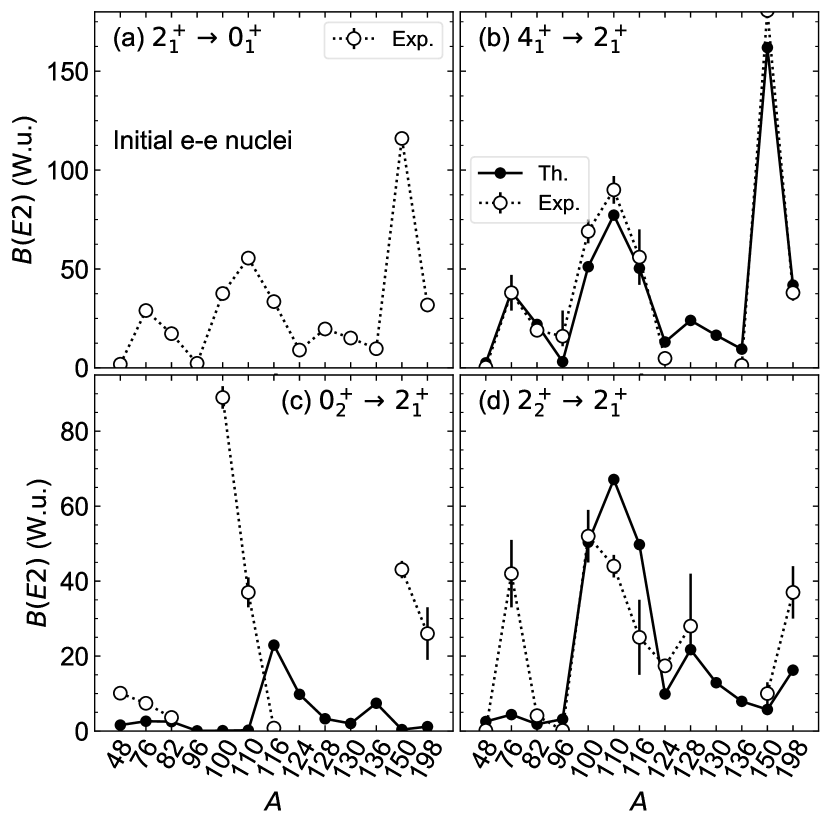
Figure 16: Theoretical and experimental $B(E2)$ transition strengths in Weisskopf units (W.u.) for the transitions (a) $2^{+}_{1}\to 0^{+}_{1}$, (b) $4^{+}_{1}\to 2^{+}_{1}$, (c) $0^{+}_{2}\to 2^{+}_{1}$ and (d) $2^{+}_{2}\to 2^{+}_{1}$ for the even-even initial nuclei with mass $A$ of the considered $2\nu\beta\beta$ decays. The experimental data are taken from Ref. [65]. The effective boson charges are adjusted to reproduce the experimental $B(E2;2^{+}_{1}\to 0^{+}_{1})$ value for each nucleus, and therefore the theoretical values are not shown in panel (a).

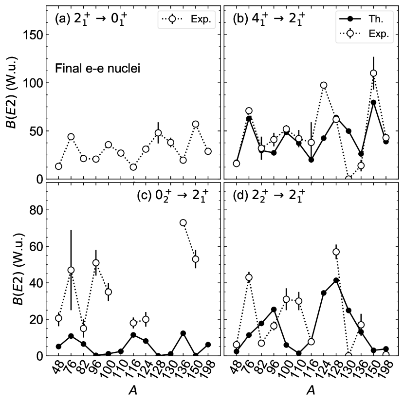
Figure 17: Same as Fig. 16, but for the even-even final nuclei of the considered $2\nu\beta\beta$ decays.

Table 17: Comparison of calculated and available experimental data for the electric quadrupole $Q(I)$ (in $e$b) and magnetic dipole $\mu(I)$ (in $\mu_{N}$) moments, and the $B(E2)$ and $B(M1)$ transition strengths (in W.u.) of the intermediate odd-odd nuclei. The relativistic functional DD-PC1 is used. The experimental values are taken from Refs. [65, 80].

Nucleus	Property	Theory	Experiment
48Sc	$\mu(6^{+}_{1})$	$+3.098$	$+3.737\pm 0.012$
76As	$\mu(1^{+}_{1})$	$+0.388$	$+0.559\pm 0.005$
96Nb	$\mu(6^{+}_{1})$	$+4.547$	$4.976\pm 0.004$
	$B(M1;5^{+}_{1}\to 4^{+}_{1})$	$+1.23$	$>0.021$
	$B(M1;2^{+}_{1}\to 3^{+}_{1})$	$+0.24$	$>0.00017$
110Ag	$\mu(1^{+}_{1})$	$+1.900$	$2.7271\pm 0.0008$
	$Q(1^{+}_{1})$	$+0.087$	$0.24\pm 0.12$
	$\mu(6^{+}_{1})$	$+3.881$	$3.589\pm 0.004$
	$Q(6^{+}_{1})$	$+0.016$	$+1.44\pm 0.10$
	$\mu(3^{+}_{1})$	$+3.438$	$3.79\pm 0.06$
	$B(M1;2^{+}_{1}\to 1^{+}_{1})$	$0.014$	$>0.033$
	$B(M1;1^{+}_{2}\;{\text{or}}\;2^{+}_{2}\to 1^{+}_{1})$	$0.27\;{\text{or}}\;0.066$	$>0.0019$
116In	$\mu(1^{+}_{1})$	$+2.478$	$2.7876\pm 0.0006$
	$Q(1^{+}_{1})$	$+0.213$	$0.11$
	$\mu(5^{+}_{1})$	$+0.177$	$4.435\pm 0.015$
	$Q(5^{+}_{1})$	$-0.813$	$+0.802\pm 0.012$
	$B(M1;4^{+}_{1}\to 5^{+}_{1})$	$0.0073$	$>0.18$
	$B(M1;2^{+}_{1}\to 1^{+}_{1})$	$0.23$	$>0.016$
	$B(M1;4^{+}_{2}\;{\text{or}}\;5^{+}_{2}\to 4^{+}_{1})$	$0.0060\;{\text{or}}\;0.062$	$0.00013\pm 0.00006$
	$B(M1;4^{+}_{2}\;{\text{or}}\;5^{+}_{2}\to 5^{+}_{1})$	$0.00019\;{\text{or}}\;0.0.028$	$0.00013\pm 0.00006$
	$B(M1;3^{+}_{1}\to 4^{+}_{1})$	$0.0090$	$>0.0080$
	$B(M1;3^{+}_{1}\to 2^{+}_{1})$	$0.11$	$>0.0066$
124Sb	$\mu(2^{+}_{1})$	$+0.849$	$-0.3\pm 0.2$
	$Q(2^{+}_{1})$	$-0.367$	$0.0\pm 0.2$
	$B(E2;3^{+}_{1}\;{\text{or}}\;4^{+}_{1}\to 5^{+}_{1})$	$3.48\;{\text{or}}\;0.34$	$0.64\pm 0.12$
130I	$\mu(5^{+}_{1})$	$+3.900$	$3.349\pm 0.007$
	$B(M1;3^{+}_{2}\to 3^{+}_{1})$	$0.0068$	$>0.0017$
	$B(M1;3^{+}_{2}\to 2^{+}_{1})$	$0.0011$	$>0.011$
	$B(M1;1^{+}_{2}\;{\text{or}}\;2^{+}_{2}\to 2^{+}_{1})$	$0.0022\;{\text{or}}\;0.022$	$>0.0026$
	$B(M1;1^{+}_{2}\;{\text{or}}\;2^{+}_{2}\to 1^{+}_{1})$	$0.00045\;{\text{or}}\;0.00058$	$>0.0046$
	$B(M1;3^{+}_{3}\to 2^{+}_{2})$	$0.0041$	$>0.0095$
	$B(M1;3^{+}_{3}\to 3^{+}_{1})$	$0.0087$	$>0.00011$
	$B(M1;3^{+}_{3}\to 2^{+}_{1})$	$0.0021$	$>0.00051$
	$B(M1;4^{+}_{2}\to 3^{+}_{1})$	$0.054$	$>0.0027$
	$B(M1;4^{+}_{2}\to 3^{+}_{2})$	$0.073$	$>0.0019$
	$B(M1;4^{+}_{2}\to 4^{+}_{1})$	$0.0045$	$>0.00050$
136Cs	$\mu(5^{+}_{1})$	$+3.570$	$+3.711\pm 0.005$
	$Q(5^{+}_{1})$	$+0.267$	$+0.225\pm 0.010$
198Au	$\mu(5^{+}_{1})$	$+6.078$	$-1.11\pm 0.02$

Figures 16 and 17 show the calculated $B(E2)$ rates between low-lying states, $B(E2;2^{+}_{1}\to 0^{+}_{1})$, $B(E2;4^{+}_{1}\to 2^{+}_{1})$, $B(E2;0^{+}_{2}\to 2^{+}_{1})$, and $B(E2;2^{+}_{2}\to 2^{+}_{1})$, in comparison with the experimental data [65]. The $B(E2;2^{+}_{1}\to 0^{+}_{1})$ and $B(E2;4^{+}_{1}\to 2^{+}_{1})$ values are generally calculated to be large, typically $>25$ W.u. Especially for open-shell nuclei such as ¹⁵⁰Nd and ¹⁵⁰Sm, the large $B(E2)$ values confirm the pronounced quadrupole collectivity. The calculated interband transitions $B(E2;0^{+}_{2}\to 2^{+}_{1})$ for both the initial and final nuclei are systematically small [Figs. 16(c) and 17(c)]. This reflects the fact that the present IBM-2 calculation generally yields a more or less rotational energy spectrum [see Fig. 3], in which this transition is rather weak. Another explanation is that the considered IBM-2 model space does not include the intruder excitation and the subsequent configuration mixing, which would have a strong influence on the nature of the $0^{+}_{2}$ state. Note that the experimental $B(E2;0^{+}_{2}\to 2^{+}_{1})$ values are quite large for some nuclei, e.g., ¹⁰⁰Mo and ⁷⁶Se. For the nuclei around these mass regions, competition between several intrinsic shapes is indeed suggested to play an important role in determining the low-lying states [84, 85]. In many of the even-even nuclei considered, the $2^{+}_{2}$ state is the bandhead of the $\gamma$-vibrational band, and thus the $2^{+}_{2}\to 2^{+}_{1}$ $E2$ transition rates are a signature of $\gamma$ softness or triaxiality. The mapped IBM-2 accounts well for the observed systematics of the $B(E2;2^{+}_{2}\to 2^{+}_{1})$ rates of the initial nuclei [Fig. 16(d)]. The predicted $B(E2;2^{+}_{2}\to 2^{+}_{1})$ values for the final nuclei, especially ¹⁰⁰Ru and ¹¹⁰Cd, are much more at variance with the data [Fig. 17(d)], probably because the triaxiality is not sufficiently taken into account for these nuclei.

Table 17 lists the calculated and experimental $Q(I)$ and $\mu(I)$ moments, and the $B(E2)$ and $B(M1)$ transition strengths for the intermediate odd-odd nuclei. The calculated $Q(I)$ and $\mu(I)$ moments are, in most cases, in a reasonable agreement with the data. However, particularly for $Q(5^{+}_{1})$ and $\mu(5^{+}_{1})$ of ¹¹⁶In, $\mu(2^{+}_{1})$ of ¹²⁴Sb, and $\mu(5^{+}_{1})$ of ¹⁹⁸Au, the IBFFM-2 values differ considerably from the observed ones in both sign and magnitude. The deviation could be explained by the structure of the relevant IBFFM-2 functions, which also points to the deficiency of the considered model space. For ¹⁹⁸Au, for instance, the $5^{+}_{1}$ ground state is mostly made of the $[\nu p_{3/2}\otimes\pi h_{11/2}]^{(J=7^{+})}$ (34 %) and $[\nu f_{5/2}\otimes\pi h_{11/2}]^{(J=3^{+})}$ (16 %) pair configurations. On the other hand, empirical studies for the low-lying structure in this mass region suggested that the $5^{+}_{1}$ state is composed mainly of the $[\nu i_{13/2}\otimes\pi d_{3/2}]^{(J=5^{+})}$ configuration, which gives rise to the correct sign of the $\mu(5^{+}_{1})$ moment [86], but which does not make any contribution in the present RHB+IBFFM-2 result. On the other hand, in the calculation based on the Gogny-D1M EDF [31] considered in Sec. V.5.2, the same quantity is calculated to be $\mu(5^{+}_{1})=-1.06$ $\mu_{N}$, which agrees with the experimental data, $-1.11\pm 0.02$ $\mu_{N}$. The $5^{+}_{1}$ wave function in this case is decomposed into the $[\nu i_{13/2}\otimes\pi s_{1/2}]^{(J=7^{+})}$ (27 %), $[\nu i_{13/2}\otimes\pi d_{3/2}]^{(J=5^{+})}$ (32 %), and $[\nu i_{13/2}\otimes\pi d_{3/2}]^{(J=7^{+})}$ (13 %) pair components, and many other small ones. Such a difference in the structure the $5^{+}_{1}$ ground-state wave function could have arisen mainly from the SPEs used in the DD-PC1 and D1M EDFs (see Table 15).

For completeness, in Table 17 a comparison is made between the calculated and experimental [65] $B(E2)$ and $B(M1)$ values of the odd-odd nuclei. In most cases, however, only the lower limit is known or the spin of the initial or final state of the transition is not firmly established, which makes it rather hard to make a meaningful comparison between theory and experiment.

References

- Avignone et al. [2008] F. T. Avignone, S. R. Elliott, and J. Engel, Rev. Mod. Phys. 80, 481 (2008).
- Ejiri et al. [2019] H. Ejiri, J. Suhonen, and K. Zuber, Phys. Rep. 797, 1 (2019).
- Primakoff and Rosen [1959] H. Primakoff and S. P. Rosen, Rep. Prog. Phys. 22, 121 (1959).
- Haxton and Stephenson [1984] W. Haxton and G. Stephenson, Prog. Part. Nucl. Phys. 12, 409 (1984).
- Doi et al. [1985] M. Doi, T. Kotani, and E. Takasugi, Prog. Theor. Phys. Suppl. 83, 1 (1985).
- Tomoda [1991] T. Tomoda, Rep. Prog. Phys. 54, 53 (1991).
- Suhonen and Civitarese [1998] J. Suhonen and O. Civitarese, Phys. Rep. 300, 123 (1998).
- Faessler and Simkovic [1998] A. Faessler and F. Simkovic, J. Phys. G: Nucl. Part. Phys. 24, 2139 (1998).
- Vogel [2012] P. Vogel, J. Phys. G: Nucl. Part. Phys. 39, 124002 (2012).
- Vergados et al. [2012] J. D. Vergados, H. Ejiri, and F. Šimkovic, Rep. Prog. Phys. 75, 106301 (2012).
- Engel and Menéndez [2017] J. Engel and J. Menéndez, Rep. Prog. Phys. 80, 046301 (2017).
- Barabash [2020] A. Barabash, Universe 6 (2020).
- Pirinen and Suhonen [2015] P. Pirinen and J. Suhonen, Phys. Rev. C 91, 054309 (2015).
- Šimkovic et al. [2018] F. Šimkovic, A. Smetana, and P. Vogel, Phys. Rev. C 98, 064325 (2018).
- Caurier et al. [2007] E. Caurier, F. Nowacki, and A. Poves, Int. J. Mod. Phys. E 16, 552 (2007).
- Yoshinaga et al. [2018] N. Yoshinaga, K. Yanase, K. Higashiyama, E. Teruya, and D. Taguchi, Prog. Theor. Exp. Phys. 2018, 023D02 (2018).
- Caurier et al. [1990] E. Caurier, A. Poves, and A. Zuker, Phys. Lett. B 252, 13 (1990).
- Caurier et al. [2012] E. Caurier, F. Nowacki, and A. Poves, Phys. Lett. B 711, 62 (2012).
- Sen’kov and Horoi [2016] R. A. Sen’kov and M. Horoi, Phys. Rev. C 93, 044334 (2016).
- Coraggio et al. [2019] L. Coraggio, L. De Angelis, T. Fukui, A. Gargano, N. Itaco, and F. Nowacki, Phys. Rev. C 100, 014316 (2019).
- Yoshida and Iachello [2013] N. Yoshida and F. Iachello, Prog. Theor. Exp. Phys. 2013, 043D01 (2013).
- Ring and Schuck [1980] P. Ring and P. Schuck, The nuclear many-body problem (Springer, Berlin, 1980).
- Bender et al. [2003] M. Bender, P.-H. Heenen, and P.-G. Reinhard, Rev. Mod. Phys. 75, 121 (2003).
- Vretenar et al. [2005] D. Vretenar, A. V. Afanasjev, G. A. Lalazissis, and P. Ring, Phys. Rep. 409, 101 (2005).
- Nikšić et al. [2011] T. Nikšić, D. Vretenar, and P. Ring, Prog. Part. Nucl. Phys. 66, 519 (2011).
- Robledo et al. [2019] L. M. Robledo, T. R. Rodríguez, and R. R. Rodríguez-Guzmán, J. Phys. G: Nucl. Part. Phys. 46, 013001 (2019).
- Nomura et al. [2008] K. Nomura, N. Shimizu, and T. Otsuka, Phys. Rev. Lett. 101, 142501 (2008).
- Brant et al. [1984] S. Brant, V. Paar, and D. Vretenar, Z. Phys. A 319, 355 (1984).
- Iachello and Van Isacker [1991] F. Iachello and P. Van Isacker, The interacting boson-fermion model (Cambridge University Press, Cambridge, 1991).
- Nomura et al. [2016a] K. Nomura, T. Nikšić, and D. Vretenar, Phys. Rev. C 93, 054305 (2016a).
- Nomura et al. [2019] K. Nomura, R. Rodríguez-Guzmán, and L. M. Robledo, Phys. Rev. C 99, 034308 (2019).
- Nomura et al. [2012a] K. Nomura, R. Rodríguez-Guzmán, L. M. Robledo, and N. Shimizu, Phys. Rev. C 86, 034322 (2012a).
- Nomura et al. [2016b] K. Nomura, T. Otsuka, and P. Van Isacker, J. Phys. G: Nucl. Part. Phys. 43, 024008 (2016b).
- Nomura et al. [2016c] K. Nomura, R. Rodríguez-Guzmán, and L. M. Robledo, Phys. Rev. C 94, 044314 (2016c).
- Nomura et al. [2013] K. Nomura, D. Vretenar, and B.-N. Lu, Phys. Rev. C 88, 021303 (2013).
- Nomura et al. [2014] K. Nomura, D. Vretenar, T. Nikšić, and B.-N. Lu, Phys. Rev. C 89, 024312 (2014).
- Nomura et al. [2016d] K. Nomura, T. Nikšić, and D. Vretenar, Phys. Rev. C 94, 064310 (2016d).
- Nomura et al. [2017] K. Nomura, T. Nikšić, and D. Vretenar, Phys. Rev. C 96, 014304 (2017).
- Nomura et al. [2020a] K. Nomura, R. Rodríguez-Guzmán, and L. M. Robledo, Phys. Rev. C 101, 024311 (2020a).
- Nomura et al. [2020b] K. Nomura, R. Rodríguez-Guzmán, and L. M. Robledo, Phys. Rev. C 101, 044318 (2020b).
- Barea and Iachello [2009] J. Barea and F. Iachello, Phys. Rev. C 79, 044301 (2009).
- Barea et al. [2013] J. Barea, J. Kotila, and F. Iachello, Phys. Rev. C 87, 014315 (2013).
- Barea et al. [2015a] J. Barea, J. Kotila, and F. Iachello, Phys. Rev. C 91, 034304 (2015a).
- Barea et al. [2015b] J. Barea, J. Kotila, and F. Iachello, Phys. Rev. D 92, 093001 (2015b).
- Deppisch et al. [2020] F. F. Deppisch, L. Graf, F. Iachello, and J. Kotila, Phys. Rev. D 102, 095016 (2020).
- Kotila and Iachello [2021] J. Kotila and F. Iachello, Phys. Rev. C 103, 044302 (2021).
- Otsuka et al. [1978a] T. Otsuka, A. Arima, and F. Iachello, Nucl. Phys. A 309, 1 (1978a).
- Van Isacker et al. [2017] P. Van Isacker, J. Engel, and K. Nomura, Phys. Rev. C 96, 064305 (2017).
- Nikšić et al. [2014] T. Nikšić, N. Paar, D. Vretenar, and P. Ring, Comput. Phys. Commun. 185, 1808 (2014).
- Nikšić et al. [2008] T. Nikšić, D. Vretenar, and P. Ring, Phys. Rev. C 78, 034318 (2008).
- Tian et al. [2009] Y. Tian, Z. Y. Ma, and P. Ring, Phys. Lett. B 676, 44 (2009).
- Bohr and Mottelson [1975] A. Bohr and B. R. Mottelson, Nuclear Structure (Benjamin, New York, 1975).
- Lalazissis et al. [2005] G. A. Lalazissis, T. Nikšić, D. Vretenar, and P. Ring, Phys. Rev. C 71, 024312 (2005).
- Otsuka et al. [1978b] T. Otsuka, A. Arima, F. Iachello, and I. Talmi, Phys. Lett. B 76, 139 (1978b).
- Dieperink et al. [1980] A. E. L. Dieperink, O. Scholten, and F. Iachello, Phys. Rev. Lett. 44, 1747 (1980).
- Ginocchio and Kirson [1980] J. N. Ginocchio and M. W. Kirson, Nucl. Phys. A 350, 31 (1980).
- Nomura et al. [2011a] K. Nomura, T. Otsuka, N. Shimizu, and L. Guo, Phys. Rev. C 83, 041302 (2011a).
- Inglis [1956] D. R. Inglis, Phys. Rev. 103, 1786 (1956).
- Beliaev [1961] S. T. Beliaev, Nucl. Phys. 24, 322 (1961).
- Nomura et al. [2012b] K. Nomura, N. Shimizu, D. Vretenar, T. Nikšić, and T. Otsuka, Phys. Rev. Lett. 108, 132501 (2012b).
- Scholten [1985] O. Scholten, Prog. Part. Nucl. Phys. 14, 189 (1985).
- Brant and Paar [1988] S. Brant and V. Paar, Z. Phys. A 329, 151 (1988).
- Iachello and Scholten [1979] F. Iachello and O. Scholten, Phys. Rev. Lett. 43, 679 (1979).
- [64] N. Yoshida, private communication (2018).
- [65] Brookhaven National Nuclear Data Center, http://www.nndc.bnl.gov.
- [66] T. Otsuka and N. Yoshida, JAERI-M (Japan At. Ener. Res. Inst.) Report No. 85 (1985).
- Nomura et al. [2010] K. Nomura, N. Shimizu, and T. Otsuka, Phys. Rev. C 81, 044307 (2010).
- Nomura et al. [2011b] K. Nomura, T. Otsuka, R. Rodríguez-Guzmán, L. M. Robledo, and P. Sarriguren, Phys. Rev. C 84, 054316 (2011b).
- Duval and Barrett [1981] P. D. Duval and B. R. Barrett, Phys. Lett. B 100, 223 (1981).
- Kremer et al. [2016] C. Kremer, S. Aslanidou, S. Bassauer, M. Hilcker, A. Krugmann, P. von Neumann-Cosel, T. Otsuka, N. Pietralla, V. Y. Ponomarev, N. Shimizu, M. Singer, G. Steinhilber, T. Togashi, Y. Tsunoda, V. Werner, and M. Zweidinger, Phys. Rev. Lett. 117, 172503 (2016).
- Bucurescu et al. [2012] D. Bucurescu, E. Drăgulescu, S. Pascu, H.-F. Wirth, D. Filipescu, G. C ăta Danil, I. C ăta Danil, D. Deleanu, K. Eppinger, T. Faestermann, D. G. Ghiţă, T. Glodariu, R. Hertenberger, M. Ivaşcu, R. Krücken, N. Mărginean, R. Mărginean, C. Mihai, A. Negret, T. Sava, L. Stroe, K. Wimmer, and N. V. Zamfir, Phys. Rev. C 85, 017304 (2012).
- Iachello and Arima [1987] F. Iachello and A. Arima, The interacting boson model (Cambridge University Press, Cambridge, 1987).
- Álvarez-Rodríguez et al. [2004] R. Álvarez-Rodríguez, P. Sarriguren, E. M. de Guerra, L. Pacearescu, A. Faessler, and F. Šimkovic, Phys. Rev. C 70, 064309 (2004).
- Griffiths and Vogel [1992] A. Griffiths and P. Vogel, Phys. Rev. C 46, 181 (1992).
- Civitarese and Suhonen [1998] O. Civitarese and J. Suhonen, Phys. Rev. C 58, 1535 (1998).
- Moreno et al. [2008] O. Moreno, R. Álvarez-Rodríguez, P. Sarriguren, E. M. de Guerra, F. Šimkovic, and A. Faessler, J. Phys. G: Nucl. Part. Phys. 36, 015106 (2008).
- Kotila and Iachello [2012] J. Kotila and F. Iachello, Phys. Rev. C 85, 034316 (2012).
- Honma et al. [2009] M. Honma, T. Otsuka, T. Mizusaki, and M. Hjorth-Jensen, Phys. Rev. C 80, 064323 (2009).
- Goriely et al. [2009] S. Goriely, S. Hilaire, M. Girod, and S. Péru, Phys. Rev. Lett. 102, 242501 (2009).
- Stone [2005] N. Stone, At. Data Nucl. Data Tables 90, 75 (2005).
- Dellagiacoma [1988] F. Dellagiacoma, Beta decay of odd mass nuclei in the interacting boson-fermion model, Ph.D. thesis, Yale University (1988).
- Dellagiacoma and Iachello [1989] F. Dellagiacoma and F. Iachello, Phys. Lett. B 218, 399 (1989).
- Nomura et al. [2020c] K. Nomura, R. Rodríguez-Guzmán, and L. M. Robledo, Phys. Rev. C 101, 014306 (2020c).
- Heyde and Wood [2011] K. Heyde and J. L. Wood, Rev. Mod. Phys. 83, 1467 (2011).
- Thomas et al. [2013] T. Thomas, K. Nomura, V. Werner, T. Ahn, N. Cooper, H. Duckwitz, M. Hinton, G. Ilie, J. Jolie, P. Petkov, and D. Radeck, Phys. Rev. C 88, 044305 (2013).
- Gao et al. [2012] B. S. Gao, X. H. Zhou, Y. D. Fang, Y. H. Zhang, S. C. Wang, N. T. Zhang, M. L. Liu, J. G. Wang, F. Ma, Y. X. Guo, X. G. Wu, C. Y. He, Y. Zheng, Z. M. Wang, S. C. Li, X. L. Yan, L. He, Z. G. Wang, Y. Zheng, F. Fang, and X. M. Chen, Phys. Rev. C 86, 054310 (2012).