Augment-Connect-Explore: a Paradigm for Visual Action
Planning with Data Scarcity

Abstract

Visual action planning particularly excels in applications where the state of the system cannot be computed explicitly, such as manipulation of deformable objects, as it enables planning directly from raw images. Even though the field has been significantly accelerated by deep learning techniques, a crucial requirement for their success is the availability of a large amount of data. In this work, we propose the Augment-Connect-Explore (ACE) paradigm to enable visual action planning in cases of data scarcity. We build upon the Latent Space Roadmap (LSR) framework which performs planning with a graph built in a low dimensional latent space. In particular, ACE is used to i) Augment the available training dataset by autonomously creating new pairs of datapoints, ii) create new unobserved Connections among representations of states in the latent graph, and iii) Explore new regions of the latent space in a targeted manner. We validate the proposed approach on both simulated box stacking and real-world folding task showing the applicability for rigid and deformable object manipulation tasks, respectively.

I Introduction

Given a start observation of the system, the goal of visual action planning [1] is to produce i) an action plan comprised of the actions required to reach a desired state, and ii) a visual plan containing observations, i.e., images, of intermediate states that will be traversed during the execution of the planned actions. In this way, the planner can be given raw image observations. This aspect is crucial in applications where the state of the system cannot be easily described analytically, as for instance in the manipulation of deformable objects like wires in manufacturing settings, clothes in fashion industries or food in agricultural setups as in the European Project CANOPIES. The supporting visual plan additionally improves the interpretability of these methods [1, 2].

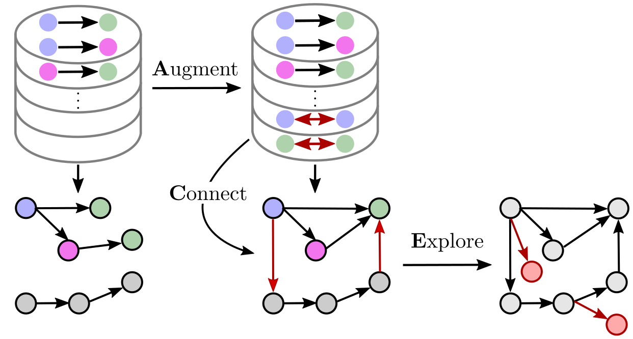
Figure 1: Overview of our ACE paradigm: (1) gaining new similar datapairs by Augmenting existing ones, (2) building unseen Connections in the latent space, and (3) efficiently Exploring new regions. Color represent the underlying states of the system (see Sec. III for details).

While it has been shown that visual dynamics used for planning can be learned directly from images, several approaches considered planning in low-dimensional latent space (discussed in Sec. II). These methods reduce the complexity of planning in the image space but generally depend on vast amount of data to train reliable policies as they require long rollouts for successful planning. In practice, this can hinder their applicability to real robotic hardware.

Therefore, in this work, we propose a method for performing visual action planning in case of data scarcity. We build upon our Latent Space Roadmap (LSR) framework [3, 4] that learns a low-dimensional latent space from input images and builds a graph, in this latent space, that is used to perform planning. We tackle data scarcity by introducing the Augment-Connect-Explore (ACE) paradigm that is based on: i) Augment: creating new informative pairs of datapoints exploiting demonstrated actions to improve the latent space structure. ii) Connect: increasing the connectivity of the LSR by building new connections, i.e. shortcuts, among nodes to improve the capability to traverse the latent space. iii) Explore: proposing targeted exploratory actions by leveraging latent representations as well as collected actions to explore new states in an efficient manner. Our contributions can be summarized as follows:

• We introduce the ACE paradigm to address data scarcity in visual action planning by augmenting, connecting and exploring.

• To realize ACE, we design a novel Suggestion Module that proposes possible actions from a given state. This is used in conjunction with a simple neural network that predicts the next latent state given the current state and desired action.

• We thoroughly analyze the individual and cumulative effects of ACE components on a simulated box stacking task and demonstrate improved performance of the combined ACE framework on a real-world folding task under data scarcity.

II Related Work

Several approaches learn the visual dynamics directly from images and use it for planning. In [1] visual foresight plans for deforming a rope into desired configurations are generated with Context Conditional Causal InfoGANs. The learned rope inverse dynamics is then considered to reach the configurations in the generated plan. In [5] Long-Short Term Memory blocks are used to compose a video prediction model predicting the stochastic pixel flow from frame to frame given the action. This model is then integrated in a Model Predictive Control (MPC) framework to produce visual plans and push objects of interest. Building on the visual foresight frameworks, the work in [6] proposes the VisuoSpatial Foresight which integrates the depth map information with the pure RGB data to learn the visual dynamic model of fabrics in a simulated environment. An extension of this approach is given in [7] where the main steps of the framework are improved.

To reduce the complexity of planning in the image space, low-dimensional latent spaces have been explored in several studies, e.g., [8]-[9]. A framework for global search in latent space is presented in [8], where motion planning is performed directly in this latent space using an RRT-based algorithm with collision checking and latent space dynamics modelled as neural networks. Contrastive learning is used in [10] to derive a predictive model in the latent space that is exploited to find rope and cloth flattening actions. Latent space goal-conditioned predictors, formulated as hierarchical models, are introduced [11] to limit the search space to trajectories that lead to the goal configuration and thus to perform long-horizon visual planning. Latent planning has also been successfully applied in Reinforcement Learning (RL) settings, like for example in [12] for model-based offline RL and in [13] for hierarchical RL. The combination of RL with graph structures in the latent space is explored in [9], where a node is created for each encoded observation. Building on [9], temporal closeness of the consecutive observations in the trajectories is also exploited in [2]. However, the above methods generally require a large amount of long rollouts for successful planning. Therefore, in this work, we tackle visual action planning for scenarios with scarce training data.

III Preliminaries and Problem Statement

In this section we provide preliminary notions for our framework and formalize the problem of visual action planning with data scarcity.

III-A Dataset structure

Let $\mathcal{O}$ be the space of all possible observations, i.e., images, of the system states. We consider a training dataset $\mathcal{T}_{o}$ consisting of $q$ tuples $(O_{1},O_{2},\mathchar 28954\relax)$, where $O_{1}$ is an observation of the start state, $O_{2}$ an observation of the successor state, and $\mathchar 28954\relax$ a variable denoting the respective action between the states. Here, an action is defined as a single transformation that brings the system to a new state different from the starting one. For example, in Fig. 2, an action corresponds to moving a box. The variable $\mathchar 28954\relax=(a,u)$ is composed of a binary variable $a\in\{0,1\}$ indicating whether or not an action occurred and a variable $u$ containing the task-dependent action-specific information in case an action occurred, i.e. $a=1$. We say that no action was performed, i.e., $a=0$, if observations $O_{1}$ and $O_{2}$ are different variations of the same (unknown) underlying state of the system. In the bottom row of Fig. 2, the observations exhibit lightning and slight positional variations, but correspond to the same underlying state of the system determined by the arrangement of the boxes. We refer to a tuple in the form $(O_{1},O_{2},\mathchar 28954\relax=(1,u))$ as an action pair and $(O_{1},O_{2},a=0)$ as a similar pair (shown in Fig. 2).

III-B Visual Action Planning

Let $\mathcal{U}$ be the set of possible actions of the system. A visual action plan is the combination of an action plan $P_{u}$ and a visual plan $P_{o}$ that lead the system from a given start $O_{s}\in\mathcal{O}$ to a goal observation $O_{g}\in\mathcal{O}$, i.e., such that $P_{o}=\{O_{s}=O_{1},O_{2},...,O_{N}=O_{g}\}$ and $P_{u}=\{u_{1},u_{1},...,u_{N-1}\}$, where $u_{n}\in\mathcal{U}$ produces a transition between consecutive observations $O_{n}$ and $O_{n+1}$ for each $n\in\{0,...,N-1\}$.

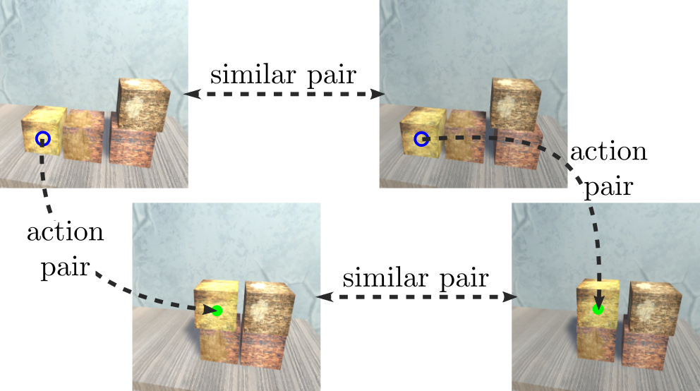
Figure 2: Examples of similar and action pairs. The similar pairs show the same underlying state, while the observations in the action pairs show different underlying states.

To reduce the complexity of the problem, we build a low-dimensional latent space $\mathcal{Z}$ encoding $\mathcal{O}$ that aims to capture the underlying states of the system.

Definition 1

The latent mapping function $\mathchar 28952\relax:\mathcal{O}\to\mathcal{Z}$ maps an observation $O_{n}\in\mathcal{O}$ into its latent representation $z_{n}\in\mathcal{Z}$. The observation generator function $\mathchar 28961\relax:\mathcal{Z}\to\mathcal{O}$ retrieves a possible observation $O_{n}\in\mathcal{O}$ associated with a latent representation $z_{n}\in\mathcal{Z}$.

Definition 2

The latent dynamic function $f:\mathcal{Z}\times\mathcal{U}\to\mathcal{Z}$ transitions the system through the latent space.

Given these functions, one way to realize visual action planning is to map the start and goal observations in the latent space, obtaining $z_{s}=\mathchar 28952\relax(O_{s})$, $z_{g}=\mathchar 28952\relax(O_{g})$, and then perform planning directly in $\mathcal{Z}$ by exploiting the latent dynamic function $f$. This leads to the definition of an action plan $P_{u}$ with corresponding latent plan $P_{z}=\{z_{s}=z_{1},z_{2},...,z_{N}=z_{g}\}$, based on which the visual plan $P_{o}$ is generated through the observation generator $\mathchar 28961\relax$. Note that in practice the functions $\mathchar 28952\relax$, $\mathchar 28961\relax$ and $f$ are unknown and need to be approximated. The quality of these approximations depends on the available amount of observations $\mathcal{T}_{o}$ of the system.

III-C Problem Statement

When $\mathcal{T}_{o}$ is scarce, it might not contain all possible latent states associated with the system as well as possible transitions among them. In this work we are interested in solving the following problem.

Problem 1

Given a scarce training dataset $\mathcal{T}_{o}$ as well as a start $O_{s}\in\mathcal{O}$ and a goal observation $O_{g}\in\mathcal{O}$, our objective is to find the related visual action plan $(P_{o},P_{u})$.

To solve it, we exploit a simple insight that two latent states are similar if the same set of actions can be applied to both, and if these, in turn, also yield the same set of consecutive states. We first define the set of actions that can be applied to a given latent state $z$.

Definition 3

A suggestion function $\mathchar 28945\relax:\mathcal{O}\to\mathcal{U}$ provides a subset $\mathchar 28945\relax(O_{i})=\mathcal{U}_{i}\subseteq\mathcal{U}$ of actions that can be applied from an observation $O_{i}\in\mathcal{O}$.

Given the suggestion function $\mathchar 28945\relax$ and latent dynamic function $f$, we define similar states as follows, in line with bisimulation theory [14].

Definition 4

The states $z_{i},z_{j}\in\mathcal{Z}$ corresponding to the observations $O_{i},O_{j}\in\mathcal{O}$ are said to be similar if

• $\mathchar 28945\relax(O_{i})=\mathchar 28945\relax(O_{j})=\widetilde{\mathcal{U}}$, and

• $\{f(z_{i},u)\}=\{f(z_{j},u)\}$ for every $u\in\widetilde{\mathcal{U}}$.

III-D Latent Space Roadmap Framework

We addressed the problem of visual action planning for scenarios of complete training datasets, i.e., those covering all possible states and transitions among them, in our earlier works [3, 4] by introducing the LSR framework, which we briefly recall in the following. The basic idea of this framework is to perform planning in the low dimensional latent space $\mathcal{Z}$ by i) structuring it to respect the underlying states of the system, and ii) building a graph directly in this latent space to guide the planning.

To address point i), we define the concept of covered regions. We map the training dataset $\mathcal{T}_{o}$ described in Section III-A into the latent space $\mathcal{Z}$ to obtain a set of covered states $\mathcal{T}_{z}=\{z_{1},...,z_{2q}\}\subset\mathcal{Z}$, i.e., $\mathcal{T}_{z}=\mathchar 28952\relax(\mathcal{T}_{o})$, for which we make the following assumption as in [3, 4].

Assumption 1

Given a covered state $z\in\mathcal{T}_{z}$, there exists $\mathchar 28962\relax>0$ such that any other state $z^{\prime}$ in the $\mathchar 28962\relax-$neighborhood $N_{\mathchar 28962\relax}(z)$ of $z$ can be considered as the same underlying state.

We define the union of $\mathchar 28962\relax$-neighbourhoods of the covered states $z\in\mathcal{T}_{z}$ as covered subspace

$$\mathcal{Z}_{sys}=\bigcup\nolimits_{z\in\mathcal{T}_{z}}N_{\mathchar 28962\relax}(z)\subset\mathcal{Z},$$ (1)

which can be rewritten as the union of $m$ path-connected components [4] called covered regions and denoted by $\{\mathcal{Z}_{sys}^{i}\}_{i=1}^{m}$. Note that in a well structured latent space, each covered region encodes a possible underlying state of the system. We define a set of transitions that connect covered regions. A covered transition function $f^{ij}_{sys}:\mathcal{Z}^{i}_{sys}\times\mathcal{U}\to\mathcal{Z}^{j}_{sys}$ maps a point $z^{i}\in\mathcal{Z}^{i}_{sys}$ to a point $z^{j}\in\mathcal{Z}^{j}_{sys}$ when applying an action $u\in\mathcal{U}$, with $i,j\in\{1,2,...,m\}$ and $i\neq j$. Given $\mathcal{Z}_{sys}$ and the covered transition functions $f^{ij}_{sys}$, we then define the Latent Space Roadmap:

Definition 5

A Latent Space Roadmap is a directed graph $LSR=(\mathcal{V}_{LSR},\mathcal{E}_{LSR})$ where each vertex $v_{i}\in\mathcal{V}_{LSR}\!\subset\!\mathcal{Z}_{sys}$ for $i\in\{1,...,m\}$ is a representative of the covered region $\mathcal{Z}^{i}_{sys}\subset\mathcal{Z}_{sys}$, and each edge $e_{i,j}=(v_{i},v_{j})\in\mathcal{E}_{LSR}$ represents a covered transition function $f^{ij}_{sys}$ between the corresponding covered regions $\mathcal{Z}^{i}_{sys}$ and $\mathcal{Z}^{j}_{sys}$ for $i\neq j$.

Two main modules compose the LSR framework. First, a Mapping Module (MM) implements the mapping function $\mathchar 28952\relax$ and observation generator $\mathchar 28961\relax$ defined in Def. 1 with a VAE framework. These are learned using a contrastive loss term, also called action term, which attracts states belonging to similar pairs and repels states belonging to action pairs to a minimum distance $d_{m}$. Second, an LSR module implements the LSR defined in Def. 5 by applying clustering in $\mathcal{Z}$ to approximate the covered regions $\mathcal{Z}^{i}_{sys}$. Each obtained cluster is associated with a node in the LSR and edges among them are created using action pairs in the training dataset $\mathcal{T}_{o}$. In this process, average action specifics are also endowed in the edges to retrieve the action plan $P_{u}$ (see the Action Averaging Baseline in [4] for details).

IV Overview of the approach

In order to perform visual planning in case of data scarcity, the proposed ACE paradigm aims to:

1. Augment the available dataset $\mathcal{T}_{o}$, autonomously creating new similar pairs.

2. Create new unobserved connections in the latent space $\mathcal{Z}$, increasing the set of covered transition functions $f^{ij}_{sys}$ and number of respective edges in the LSR.

3. Explore new regions of $\mathcal{Z}$ in an efficient and guided manner, increasing the covered subspace $\mathcal{Z}_{sys}$.

To realise the ACE paradigm we extend the LSR framework with a Latent Prediction Model (LPM) and a Suggestion Module (SM). An overview of the overall ACE architecture including all the modules is shown in Fig. 3. We mark in green the modules used at run time to produce the visual action plan (bottom) from start $O_{s}$ and goal observations $O_{g}$ (left), and in grey the ones only used offline.

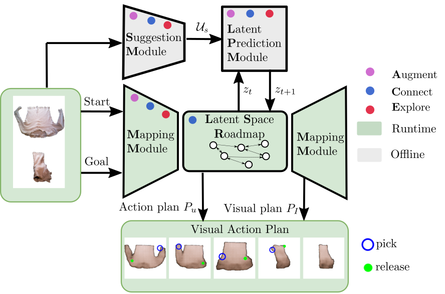
Figure 3: Overview of the proposed architecture for visual action planning. The modules involved in the ACE phases are highlighted with respective colored dots. The modules only used offline are marked in grey, while the ones also used online are marked in green.

The LPM module approximates the latent dynamics function in Def. 2 which, given a latent state $z_{i}$ and an action $u\in\mathcal{U}$, predicts a potential next state $z_{i+1}$. Note that LPM implicitly assumes a given MM. The SM module approximates the suggestion function $\mathchar 28945\relax$ in Def. 3 and, given an observation $O_{i}$, suggests a set of potential actions $\mathcal{U}_{i}$ that are possible to perform. The input image $O_{i}$ can be either an observation of the current state or an observation generated by $\mathchar 28961\relax$.

To realize point 1), we rely on the definition of similar states in Def. 4 and employ SM and LPM to find novel similar pairs that are added to $\mathcal{T}_{o}$ to obtain the augmented training dataset $\overline{\mathcal{T}_{o}}$. The latter is then used to obtain a new mapping function approximation ${\mathchar 28952\relax}$ by updating the MM, which leads to an enhanced structure of the latent space $\mathcal{Z}$.

Regarding point 2), we use SM and LPM along with the covered subspace $\mathcal{Z}_{sys}$ to identify previously unseen transitions $f^{ij}_{sys}$ that are possible to execute, called valid transitions. These are added to the LSR in the form of new edges referred to as shortcuts.

Similarly, point 3) is realized by using the SM, that suggests the set of possible actions $\mathcal{U}_{i}$ from the current state $z_{i}$, and the LPM that predicts potential next states. Among the possible actions, the most promising one is chosen for exploration, as described in Sec. V-C. This enables exploring new regions of the latent space $\mathcal{Z}$ in a guided manner.

The ACE paradigm improves the individual components of the LSR framework which is then used to perform visual action planning. Note that even though we focus on the LSR framework, ACE is general and applicable to many other contexts, e.g., the proposed targeted exploration approach can be easily integrated into an RL setting.

IV-A Models for LPM and SM

We model LPM as a simple multilayer perceptron (MLP), as detailed in Sec. VI. During augmentation and connection phases, we also leverage the covered subspace $\mathcal{Z}_{sys}$ defined in (1): we consider a state $z_{j}$ predicted by the LPM reliable only if it falls within the covered subspace, i.e., $z_{j}\in\mathcal{Z}_{sys}$. We refer to the LPM including the covered subspace check as reliable LPM (LPM-R) in the following.

The SM is built based on two core considerations: i) several valid actions can be applied to the same state, and ii) the same action can be applied to different states. We model the suggestion function $\mathchar 28945\relax$ with a Siamese network trained with a contrastive loss that encourages clustering of the states from which the same subset of actions can be performed.

In detail, we build the training dataset for the SM, denoted by $\mathcal{T}^{SM}_{o}$, by rearranging the observations in the training tuples in $\mathcal{T}_{o}$ depending on the actions. A similar pair $(O_{1},O_{2},s=1)$, where $s$ is the similarity signal, is added to $\mathcal{T}^{SM}_{o}$ if the same action specifics $u$ is applied from $O_{1}$ and $O_{2}$ in $\mathcal{T}_{o}$, i.e., if there exist $(O_{1},-,\mathchar 28954\relax=(1,u))\in\mathcal{T}_{o}$ and $(O_{2},-,\mathchar 28954\relax=(1,u))\in\mathcal{T}_{o}$, where $-$ denotes any other observation. On the other hand, a dissimilar pair $(O_{1},O_{2},s=0)$ is added to $\mathcal{T}^{SM}_{o}$ when different action specifics are applied from $O_{1}$ and $O_{2}$ in $\mathcal{T}_{o}$, i.e., if there exist $(O_{1},-,\mathchar 28954\relax=(1,u_{1}))\in\mathcal{T}_{o}$ and $(O_{2},-,\mathchar 28954\relax=(1,u_{2}))\in\mathcal{T}_{o}$ with $u_{1}\neq u_{2}$. Note that training the Siamese network with the dataset $\mathcal{T}^{SM}_{o}$ results in a latent space $\mathcal{Z}^{\prime}$ different from $\mathcal{Z}$. The latent space $\mathcal{Z}^{\prime}$ is then clustered and each cluster $\mathcal{C}\subset\mathcal{Z}^{\prime}$ is labeled with the set $\mathcal{U}_{c}\subseteq\mathcal{U}$ containing all the actions that are executed starting from the states points in $\mathcal{C}$. We experimentally validate that the above procedure allows to achieve a good approximation of the suggestion function despite some possible erroneous similarity signals in $\overline{\mathcal{T}}_{o}^{SM}$.

At run time, a novel observation $O_{i}$ is fed into the Siamese network to obtain its latent representation $z_{i}^{\prime}\in\mathcal{Z}^{\prime}$ and the set of suggested actions $\mathcal{U}_{i}$ associated with the closest cluster $\mathcal{C}_{i}$ as visualized in Fig. 4.

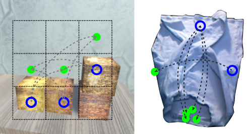
Figure 4: Example of the set of suggested actions $\mathcal{U}$ using the SM for a box stacking (left) and T-shirt folding (right) task. The blue rings mark pick locations, while the green circles place locations.

V ACE Paradigm

In this section we present the individual components of our ACE paradigm and provide an overview of the full framework.

V-A Augment

The proposed augmentation procedure builds new similar pairs based on the definition in Def. 4. In particular, if the same set of actions applied from different observations $O_{1}$ and $O_{2}$ leads to the same underlying states, we consider the two starting observations as a similar pair. In doing so, we discover similar pairs among states that are erroneously further apart in the latent space $\mathcal{Z}$. This occurs in practice since the latent mapping $\mathchar 28952\relax$ is only an approximation. Therefore, to improve the structure of $\mathcal{Z}$, it is crucial to identify more similar pairs in the dataset $\mathcal{T}_{o}$ such that ${\mathchar 28952\relax}$ is re-learned to map the same underlying states close together.

Note that no labels about the underlying states contained in the training observations, that could be exploited for augmenting the dataset, are provided. In contrast, we only have access to the information of whether two observations are similar or there is an action between them.

Algorithm 1 Augmentation Algorithm

Training dataset $\mathcal{T}_{o}$, search radius $r$

1:$\mathcal{T}_{z}\leftarrow\text{MM}(\mathcal{T}_{o})$

2:$\overline{\mathcal{T}}_{o}:={\mathcal{T}}_{o}$

3:for each $z_{i}\in\mathcal{T}_{z}$ do

4:    $\mathcal{U}_{i}\leftarrow\text{SM}(O_{i})$

5:    $\mathcal{L}_{i}\leftarrow\text{search in radius}(\mathcal{T}_{z},z_{i},r)$

6:    $\mathcal{L}_{i}\leftarrow\text{descent sort}(\mathcal{L}_{i})$

7:    found := False

8:    for each $z_{j}\in\mathcal{L}_{i}$ and not found do

9:         $O_{j}\leftarrow\text{get observation}(\mathcal{T}_{o},j)$

10:         $\mathcal{U}_{j}\leftarrow\text{SM}(O_{j})$

11:         if $\mathcal{U}_{i}\equiv\mathcal{U}_{j}$ then

12:             $\mathcal{Z}^{p}_{i},\mathcal{Z}^{p}_{j}\leftarrow\text{LPM-R}(z_{i},\mathcal{U}_{i}),\text{LPM-R}(z_{j},\mathcal{U}_{i})$

13:             $\mathcal{Z}^{n}_{i},\mathcal{Z}^{n}_{j}\leftarrow\text{nearest}(\mathcal{T}_{z},\mathcal{Z}^{p}_{i}),\text{nearest}(\mathcal{T}_{z},\mathcal{Z}^{p}_{j})$

14:             if  $\mathcal{Z}^{n}_{i}\equiv\mathcal{Z}^{n}_{j}$ then

15:                 $\bar{\mathcal{T}}_{o}:=\overline{\mathcal{T}}_{o}\cup\{\left(O_{i},O_{j},a=0\right)\}$

16:                 found := True                           

return $\bar{\mathcal{T}}_{o}$

Algorithm 1 summarizes the augmentation procedure. Given the training dataset $\mathcal{T}_{o}$ and a search radius $r$ determining the search area around covered states, we encode all observations $O_{i}\in\mathcal{T}_{o}$ to obtain $\mathcal{T}_{z}\subset\mathcal{Z}$ (line 1) and initialize the augmented dataset $\overline{\mathcal{T}}_{o}$ (line 2). For each latent state $z_{i}\in\mathcal{T}_{z}$, we check if a new similar pair can be identified. We first obtain the set $\mathcal{U}_{i}$ of possible actions from $z_{i}$ using the SM (line 4). Then, we define the set $\mathcal{L}_{i}$ of covered latent states which are within the search radius $r$ (line 5), i.e., $\mathcal{L}_{i}=\{z_{j}\in\mathcal{T}_{z}\,|\,z_{j}\in{N}_{r}(z_{i})\}$. This is followed by a descent sorting with respect to the distance of each $z_{j}\in\mathcal{L}_{i}$ to $z_{i}$ (line 6). Note that we limit the search in a radius only for computational reasons. Since the latent space $\mathcal{Z}$ already has a certain structure inferred from the non-augmented dataset $\mathcal{T}_{o}$ during training of MM, we avoid checking states that are too far away from the current and likely not similar to it.

At this point, we analyze the covered states $z_{j}\in\mathcal{L}_{i}$. Starting from the first $z_{j}$, we take the corresponding observation $O_{j}$ in the training dataset (line 9) and obtain the set of potential actions $\mathcal{U}_{j}$ (line 10). If all the actions in the sets $\mathcal{U}_{i},\,\mathcal{U}_{j}$ coincide, we obtain the sets of respective predicted states $\mathcal{Z}^{p}_{i},\mathcal{Z}^{p}_{j}$ (line 12) by the LPM-R, which checks the reliability condition discussed in Sec. IV-A. Based on these sets, the sets $\mathcal{Z}^{n}_{i},\mathcal{Z}^{n}_{j}$ consisting of closest covered latent states in $\mathcal{T}_{z}$ with respect to $\mathcal{Z}^{p}_{i},\mathcal{Z}^{p}_{j}$, respectively, are found. If $\mathcal{Z}^{n}_{i},\mathcal{Z}^{n}_{j}$ coincide, a new similar pair $(O_{i},O_{j},a=0)$ is added to the augmented dataset $\overline{\mathcal{T}}_{o}$, otherwise the next state $z_{j}\in\mathcal{L}_{i}$ is analyzed.

V-B Connect

A good connectivity of nodes is essential for the success of graph-based planning methods. Although more connections can be built by collecting more data, a more efficient approach involves building shortcuts, i.e., connections between nodes that are not directly induced by the training set. In this work, we infer them by using the SM and LPM modules. Note that it is crucial to add correct shortcuts as erroneous connections can be very detrimental for the graph planning capabilities, leading to unfeasible plans.

Algorithm 2 Connection Algorithm

${LSR}=(\mathcal{V}_{LSR},\mathcal{E}_{LSR})$, neighborhood size $\mathchar 28962\relax$

1:for each $z_{i}\in\mathcal{V}_{LSR}$ do

2:    $O_{i}\leftarrow\text{MM}(z_{i})$

3:    $\mathcal{U}_{i}\leftarrow\text{SM}(O_{i})$

4:    for each  $u\in\mathcal{U}_{i}$ do

5:         $z_{n}\leftarrow\text{LPM}(z_{i},u)$

6:         if $\|z_{j}-z_{n}\|_{1}<\mathchar 28962\relax\text{ for }z_{j}\in\mathcal{V}_{LSR},i\neq j$ then

7:             $\mathcal{E}_{{LSR}}\leftarrow$ create edge ($z_{i},z_{j},u$)              

return $LSR$

Algorithm 2 summarizes the proposed method for building shortcuts. The basic idea is that if an action $u$ suggested by the SM in a certain state $z_{i}$ leads to a covered state $z_{j}$, then the respective transition can be considered as valid and can be added to the LSR. In detail, given the LSR and the neighborhood size $\mathchar 28962\relax$, we iterate over the states in the set of nodes $\mathcal{V}_{LSR}$ of the LSR. For each state $z_{i}$ in $\mathcal{V}_{LSR}$, we generate the respective observation $O_{i}$ through the observation generator $\mathchar 28961\relax$ of the MM (line 2) and obtain the set of potential actions $\mathcal{U}_{i}$ by the SM. For each $u\in\mathcal{U}_{i}$, LPM predicts the next state $z_{n}$ obtained from $z_{i}$ (line 5). If the predicted next state $z_{n}$ falls in the $\mathchar 28962\relax$-neighborhood of any other state $z_{j}\in\mathcal{V}_{LSR}$ in the LSR with $i\neq j$, an edge between $z_{i}$ and $z_{j}$ is added in the edge set $\mathcal{E}_{LSR}$ of the LSR (line 7). We also endow the edge with the new predicted action $u$ for action planning purposes as discussed in III-D.

V-C Explore

The challenges of finding suitable actions for exploration of the latent space $\mathcal{Z}$ are twofold: i) finding valid actions that can be performed in the current state, and ii) choosing the action that is most beneficial to the system.

The SM model provides a solution to the first problem as it outputs a set of valid actions $\mathcal{U}_{i}$ for an observation $O_{i}$ corresponding to the current state $z_{i}$ as described in Sec. IV-A. For the second problem, we propose to undertake the action that leads to the most unexplored area of the latent space $\mathcal{Z}$ at each exploration step.

The approach is summarized in Algorithm 3. Given the training dataset $\mathcal{T}_{z}$ and the current state observation $O_{i}$, we first map both into $\mathcal{Z}$ with the mapping function $\mathchar 28952\relax$ of the MM (lines 1-2). Then, we retrieve the set of potential actions $\mathcal{U}_{i}$ from the current state $z_{i}$ through the SM. We initialize an empty auxiliary exploration list $\mathcal{L}_{e}$. For each action $u\in\mathcal{U}_{i}$, we predict the next state $z_{n}$ using the LPM (line 6) and compute the distance $d_{i}$ from $z_{i}$ to the nearest covered state in $\mathcal{T}_{z}$ (line 7). The tuple given by the action $u$ and distance $d_{i}$ is added to the exploration list $\mathcal{L}_{e}$. Once all the actions in $\mathcal{U}_{i}$ have been analyzed, we return the action $u_{e}$ (line 9) that leads to the furthest latent state as the exploratory one. As described in the following, the observation $O_{i+1}$ obtained after executing $u_{e}$ is used to create a new action pair $(O_{i},O_{i+1},\mathchar 28954\relax=(1,u_{e}))$ that is added to $\mathcal{T}_{o}$. The latent space is explored by executing Algorithm 3 $n_{e}$ times. Note that in case the LPM does not provide an accurate prediction for unseen states, this would only result in computing an imprecise distance $d_{i}$, and then choosing a less beneficial action to explore.

Algorithm 3 Exploration Algorithm

Training dataset $\mathcal{T}_{o}$, current observation $O_{i}$

1:$\mathcal{T}_{z}\leftarrow\text{MM}(\mathcal{T}_{o})$

2:$z_{i}\leftarrow\text{MM}(O_{i})$

3:$\mathcal{U}_{i}\leftarrow\text{SM}(O_{i})$

4:$\mathcal{L}_{e}$ := $\{\}$

5:for each $u\in\mathcal{U}_{i}$  do

6:    $z_{n}\leftarrow\text{LPM}(z_{i},u)$

7:    $d_{i}\leftarrow\text{nearest}(\mathcal{T}_{z},z_{n})$

8:    $\mathcal{L}_{e}\leftarrow\text{add tuple}(u,d_{i})$

9:$u_{e}\leftarrow\text{get action to furthest state}(\mathcal{L}_{e})$

return $u_{e}$

V-D LSR with ACE

In this section, we describe how the ACE components are combined within the LSR framework, summarized in Algorithm 4. Given an initial training dataset $\mathcal{T}_{o}$, the hyperparameters $r$ and $\mathchar 28962\relax$ as well as the number of total exploration steps $n_{e}$, we first build the models employed in the ACE paradigm (line 1). Secondly, we generate the augmented dataset $\overline{\mathcal{T}_{o}}$ following Algorithm 1 with the search radius $r$ and use it to update the MM, LPM, and SM models. Thirdly, we perform the targeted exploration phase. For each exploration step $i\in\{1,...,n_{e}\}$, we get the current observation $O_{i}$, determine the most promising exploration action $u_{e}$ using Algorithm 3 (line 6) and execute it (line 7) to reach the new observation $O_{i+1}$. The observed tuple $\left(O_{i},O_{i+1},(\mathchar 28954\relax=(1,u_{e}))\right)$ is added to the dataset $\overline{\mathcal{T}_{o}}$ (line 8). After completing the exploration, the LSR is built using the approach in [3] with neighborhood threshold $\mathchar 28962\relax$ (line 9). Finally, we add the shortcuts as in Algorithm 2 (line 10) and the final LSR is returned. In case the system performance after executing Algorithm 4 is not satisfactory, this can be repeated multiple times to further improve the results.

Algorithm 4 Integration Algorithm

Training dataset $\mathcal{T}_{o}$, search radius $r$, neighborhood threshold $\mathchar 28962\relax$, number of explorations $n_{e}$

1:MM, LPM, SM $\leftarrow$ build models$(\mathcal{T}_{o})$

2:${\overline{\mathcal{T}}}_{o}\leftarrow\text{augment dataset}(\mathcal{T}_{o},r)$ [Alg. 1]

3:MM, LPM, SM $\leftarrow$ update models$({\overline{\mathcal{T}}}_{o})$

4:for each $i\in\{1,..,n_{e}\}$ do

5:    $O_{i}\leftarrow\text{current observation}$

6:    $u_{e}\leftarrow\text{get exploration action}({\overline{\mathcal{T}_{o}}},O_{i})$ [Alg. 3]

7:    $O_{i+1}\leftarrow\text{perform action}(u_{e})$

8:    ${\overline{\mathcal{T}_{o}}}:={\overline{\mathcal{T}_{o}}}\cup\{\left(O_{i},O_{i+1},(\mathchar 28954\relax=(1,u_{e}))\right)\}$

9:$LSR\leftarrow\text{build LSR}({\overline{\mathcal{T}_{o}}},\mathchar 28962\relax)$ [3]

10:$LSR_{ace}\leftarrow\text{build shortcuts}(LSR,\mathchar 28962\relax)$ [Alg. 2]

return $LSR_{ace}$

VI Simulation results

To validate the proposed approach, we consider a simulated box stacking task, shown in Fig. 2 and referred to as hard stacking task in [4]. This setting allows to determine the true underlying state of each observation (exploited for evaluation purposes only) and therefore to automatically validate the effectiveness of each ACE component as well as of the entire ACE framework.

The box stacking task is composed of a $3\times 3$ grid where four boxes can be stacked on top of each other. The underlying state is defined by the geometrical arrangement of the boxes, where each box is considered unique. The action specifics $u$ is represented by the pick and place coordinates. In each observation, we induce different lighting conditions as well as $\approx 17\%$ random noise in the positioning of the boxes in each cell. The following rules apply: i) only one box can be moved at the time, ii) only one box can be placed in a single grid cell, iii) boxes cannot float, and iv) a box can only be picked if no other box is on top of it. Given the $3\times 3$ grid and the above rules, the system exhibits exactly $288$ possible underlying states, and $|\mathcal{U}|=48$ possible actions.

VI-A Evaluation Criteria and Implementation Details

To evaluate the effectiveness of the ACE paradigm in scarce data settings, we randomly sub-sample $80\%$, $75\%$, $60\%$, $50\%$, $40\%$, and $30\%$ of the original dataset $\mathcal{T}_{100}$ [4] consisting of $2500$ pairs. We denote these sub-sampled dataset as $\mathcal{T}_{80}$, $\mathcal{T}_{75}$, $\mathcal{T}_{60}$, $\mathcal{T}_{50}$, $\mathcal{T}_{40}$, and $\mathcal{T}_{30}$, respectively. We compare the combined ACE-LSR with the $\mathchar 28962\relax$-LSR in [3] as well as with the ablated versions of each component of ACE, namely A-LSR for the augmentation step, C-LSR for connection step, and E-LSR for the exploration step. We additionally implement: i) a baseline augmentation step, referred to as A_b-LSR, which generates similar pairs using the closest states in the latent space, and ii) a baseline exploration step, referred to as E_b-LSR, which is a random explorer selecting a random action from the set $\mathcal{U}$ of the system actions and trying to apply it to the given state observation. For the sake of space, we omit the comparison of ACE-LSR to other existing methods, but this can be found for the general LSR framework in [4].

We score all frameworks by the planning performance on $1000$ novel start and goal states randomly selected from a holdout dataset composed of $2500$ observations. We report the percentage of correct transitions, and the percentage of cases where all plans are correct, and where at least one of the suggested plan is correct, denoted by % trans., % all, and % any, respectively. Furthermore, to evaluate the augmentation component, we report the number of newly identified similar pairs, # pairs, and the percentage of correct pairs among them, % pairs, using the ground truth underlying states. The connection component is similarly scored by measuring the number of new edges built in the graph, # edges, as well as the percentage of correct edges, % edges. Finally, the exploration component is evaluated by performing $n_{e}=500$ exploration steps from random initial states and defining the percentage of valid exploratory actions, % explore. For each score, we report mean and variance obtained with three different seeds for the MM model training.

The VAE modelling the MM is trained as in [4] with latent dimension $16$. A DBSCAN-based [15] clustering algorithm is used for building the LSR. The hyperparameter $\mathchar 28962\relax$ is set to $\mathchar 28962\relax=\mathchar 28950\relax_{0}+w_{\mathchar 28962\relax}\cdot\mathchar 28955\relax_{0}$ as in [3] where $\mathchar 28950\relax_{0}$ and $\mathchar 28955\relax_{0}$ are the mean and standard deviation of the $L_{1}$ distances $\|z_{1}-z_{2}\|_{1}$ among similar latent pairs $(z_{1},z_{2},a=0)$, respectively, and $w_{\mathchar 28962\relax}$ is a scaling parameter. We perform a grid search for $w_{\mathchar 28962\relax}$ in the interval $[-0.65,-0.05]$ with step size $0.1$. The LPM is a two-layer, 100 nodes MLP, while the Siamese network for the SM is a shallow two convolutional layer network with a latent space dimension $12$ as in [16]. We train the Siamese network for $100$ epochs and perform HDBSCAN [17] clustering in the latent space $\mathcal{Z}^{\prime}$ of the model. We set search radius $r=\mathchar 28950\relax_{0}$ in Algorithm 1 since similar states should generally fall at a distance equal to the mean of similar states in the training dataset. While performing exploration, we additionally remove the action obtained by reversing the last action from the set of possible actions and apply a reset of the system state each time an invalid action is undertaken.

VI-B Evaluation Results

Framework	# pairs	% pairs	# edges	% edges	% explore	% trans.	% all	% any
$\mathchar 28962\relax$-LSR [3]	$-$	$-$	$-$	$-$	$-$	$60.5\pm 4.4$	$49.1\pm 5.9$	$49.6\pm 5.7$
Ab-LSR	$1654\pm 9.0$	$95.18$	$-$	$-$	$-$	$58.8\pm 5.7$	$32.3\pm 19.2$	$33.1\pm 19.2$
A-LSR	$15\pm 11.0$	$100$	$-$	$-$	$-$	$64.0\pm 13.5$	$56.5\pm 12.1$	$56.8\pm 12.3$
C-LSR	$-$	$-$	$479.2\pm 52.1$	$95.1\pm 0.4$	$-$	$87.7\pm 0.6$	$57.1\pm 9.4$	$63.0\pm 7.9$
Eb-LSR	$-$	$-$	$-$	$-$	$7.8\pm 0.0$	$65.9\pm 0.2$	$51.4\pm 5.7$	$52.3\pm 5.3$
E-LSR	$-$	$-$	$-$	$-$	$97.7\pm 0.4$	$80.7\pm 2.0$	$62.2\pm 3.0$	$65.7\pm 3.1$
ACE-LSR	$15\pm 11.0$	$100$	$401.0\pm 15.3$	$96.6\pm 1.0$	$97.1\pm 1.6$	$93.1\pm 1.9$	$79.2\pm 4.2$	$82.6\pm 4.0$

Table I: Evaluation results obtained on the box stacking task with $\mathcal{T}_{50}$ using $\mathchar 28962\relax$-LSR as well as its combination with the baseline augmentation and exploration methods, the individual components of ACE paradigm and all the ACE components. The symbol $-$ denotes that the respective score is not relevant to the framework. See Sec. VI-A for details. Best results in bold.

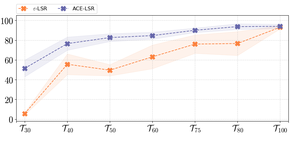
Figure 5: Planning performance on the box stacking task in terms of % any using $\mathchar 28962\relax$-LSR [3] (orange) and ACE-LSR (blue) trained on the subsampled datasets.

Figure 5 shows the planning performance in terms of % any score across the considered subsampled datasets when the proposed ACE paradigm is used (blue) and not (orange). Cross marks denote mean values, while the transparency represents the variance. We can observe that ACE-LSR boosts the planning performance compared to the $\mathchar 28962\relax$-LSR [3] for each subsampled dataset and is particularly essential in case of very scarce datasets, e.g. $\mathcal{T}_{30}$-$\mathcal{T}_{50}$. For example, average improvements equal to $\approx 45,\,21,\,33\%$ are observed for $\mathcal{T}_{30}$,$\mathcal{T}_{40}$,$\mathcal{T}_{50}$, reaching $\approx 51.5,76.5,82.6\%$, respectively. Obviously, the improvement is much more significant with scarce datasets, while the performance is almost saturated with $\mathcal{T}_{100}$, reaching $93\%$ and $94\%$ with $\mathchar 28962\relax$-LSR and ACE-LSR, respectively.

Table I shows the results of the ablation study for the components of the ACE paradigm compared with the $\mathchar 28962\relax$-LSR. We report the complete scoring described in Sec. VI-A obtained using $\mathcal{T}_{50}$ which consists of half the data used in [3]. We observe that data scarcity leads to unsatisfactory planning performance of the $\mathchar 28962\relax$-LSR, reaching only average % any score of $49.6\%$ with % trans equal to $60.5\%$. No improvement but rather a decrease of performance is recorded with the baseline augmentation step, i.e., with A_b-LSR (row 2). This builds $1654$ new similar pairs among which $\approx 95\%$ are correct. However, these new pairs deteriorate the structure of the latent space, resulting in % any equal to $33.1\%$ only with a decrease of $\approx 16\%$. This suggests that simply adding new correct pairs does not necessarily induce improved performance if they are not carefully selected. In contrast, our augmentation algorithm A-LSR (row 3) produces only $15$ new similar pairs on average that are $100\%$ correct, thus boosting the planning performance in terms of % any to average $56.8\%$. Our connection algorithm in C-LSR (row 4). builds $\approx 479$ new shortcuts that are $\approx 95\%$ correct. These yield to much higher planning scores, reaching average $87.7\%$ and $63\%$ for % trans. and % any, respectively. Concerning the exploration phase, only $7.8\%$ of the moves (% explore score) attempted by the baseline random explorer in E_b-LSR (row 5) are correct. This results in $\approx 2.5$ percentage point enhancement of the planning performance in terms of % any compared to $\mathchar 28962\relax$-LSR. On the other hand, a substantial improvement in planning performance is recorded when employing our exploration algorithm E-LSR (row 6). More specifically, $\approx 97.7\%$ of the $n_{e}=500$ exploration moves are found to be valid, resulting in average $80.7\%$ and $65.7\%$ for % trans. and % any scores, respectively. This result suggests the effectiveness of the proposed SM models for proposing exploration actions, which are found almost always to be correct. Examples of suggested actions by the SM for the stacking task are reported in Fig. 4-left. Finally, the combined ACE-LSR approach (row 7) significantly outperforms all of the above mentioned frameworks, leading to an improvement $>30\%$ in terms of % trans.,% all,% any compared to the $\mathchar 28962\relax$-LSR and reaching a final % any performance of $82.6\%$.

VII Experimental Results

To further validate the effectiveness of the ACE paradigm, we perform a real world T-shirt folding task as in [3]. In this task, the goal is to generate and execute visual action plans from a start configuration to five different goal configurations, shown in Fig. 6.

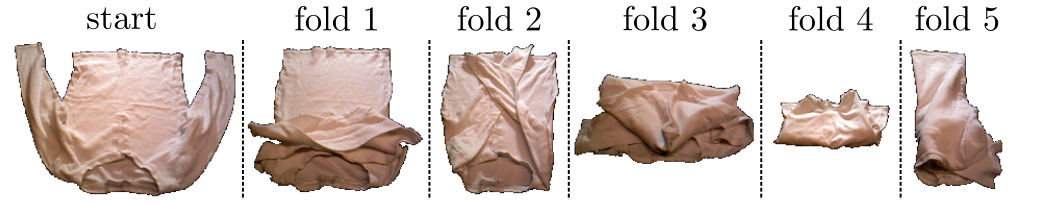
Figure 6: Start and five goal configurations of the T-shirt.

Let $\mathcal{F}_{100}$ be the training dataset used in [3] containing a total of $1150$ pairs, and let $\mathcal{F}_{50}\subset\mathcal{F}_{100}$ be a scarce dataset consisting of $50\%$ randomly subsampled pairs. We use the same set of parameters and architectures as in Sec. VI-A unless otherwise specified. Since the action specifics $u$ is composed of pixel position pick and place coordinates, the action space is much larger as in the simulation task. In order for the SM to be able to suggest meaningful actions, we discretize the action space into bins and use the mean actions of each bin. We choose a bin size of $\approx 15\%$ of the image space which results in $107$ unique actions. Furthermore, we group the observations only based on the similarity of the pick action as this enables more flexible exploration. Examples of suggested actions for the T-shirt folding task are shown in Fig. 4-right. The SM, trained for $200$ epochs, is then used in the augmentation step obtaining $13$ new similar pairs (Algorithm 1). When applying the connection algorithm using the SM and LPM-R we obtain $55$ novel edges in the graph. In order to obtain more novel connections, we increase the LPM-R reliability check by a factor of $1.5$ since both the scarcity and diversity of the actions make a reliable prediction more challenging. Lastly, we execute Algorithm 3 for $n_{e}=20$ exploration steps. Note that exploration in the folding task is much less constrained, and therefore some explorations can lead to completely novel folding sequences not observed in the collected training dataset $\mathcal{T}_{o}$. Including the newly obtained action pairs yields the final ACE-LSR (built with $w_{\mathchar 28962\relax}=1$) that we compare with $\mathchar 28962\relax$-LSR ($w_{\mathchar 28962\relax}=1.4$) trained on $\mathcal{F}_{50}$ in Tab. I. We repeat each fold five times and report the number of successful trials when the entire fold is performed successfully. The execution videos, visual action plans as well as the exploration can be seen on the project website. Moreover, an example of a generated visual action plan is provided in Fig. 3.

The ACE-LSR outperforms the $\mathchar 28962\relax$-LSR in all folds except for fold $4$, and reaches a total system success rate over all five folds of $80\%$, matching the performance reported in [3] using only half the training data. We observe that the $\mathchar 28962\relax$-LSR does not have enough data to distinguish fold $1$ from fold $2$ as it always performs fold $2$ regardless of the fold goal state. On the contrary, ACE-LSR is able to successfully distinguish them and execute the correct fold most of the times. Furthermore, the $\mathchar 28962\relax$-LSR is not able to reliably execute fold $5$ as it is missing the final step to complete it, while ACE-LSR is able to perform it in $4/5$ cases.

Framework	fold 1	fold 2	fold 3	fold 4	fold 5
$\mathchar 28962\relax$-LSR	$0/5$	$5/5$	$0/5$	$5/5$	$1/5$
ACE-LSR	$4/5$	$5/5$	$3/5$	$4/5$	$4/5$

Table II: System performance results on the T-shirt folding task with $\mathcal{F}_{50}$ for $\mathchar 28962\relax$-LSR and ACE-LSR on five different folds, each repeated five times. Best results in bold.

VIII Conclusions

In this work, we presented the ACE paradigm that addresses data scarcity problem for visual action planning. We built upon the Latent Space Roadmap framework and introduced i) a novel Suggestion Model (SM), that given an observation, suggests possible actions in that state, and ii) a Latent Prediction Model (LPM) that, given a latent state and an action, predicts the next latent state. Combining these modules, we Augmented the dataset to identify new similar pairs for training, identified new valid edges in the LSR to increase its Connectivity, and Explored the latent space efficiently to reach potential undiscovered states. We validated the ACE paradigm on a simulated box stacking task and a real-world T-shirt folding task on several levels of data scarcity. As future work, we aim to extend this paradigm to different contexts, such as RL.

References

- [1] Angelina Wang, Thanard Kurutach, Pieter Abbeel and Aviv Tamar “Learning Robotic Manipulation through Visual Planning and Acting” In Robotics: Science and Systems, 2019
- [2] Kara Liu, Thanard Kurutach, Christine Tung, Pieter Abbeel and Aviv Tamar “Hallucinative Topological Memory for Zero-Shot Visual Planning” In Int. Conf. Mach. Learn., 2020, pp. 6259–6270
- [3] Martina Lippi, Petra Poklukar, Michael C Welle, Anastasiia Varava, Hang Yin, Alessandro Marino and Danica Kragic “Latent Space Roadmap for Visual Action Planning of Deformable and Rigid Object Manipulation” In IEEE/RSJ Int. Conf. on Intelligent Robots and Systems, 2020
- [4] Martina Lippi, Petra Poklukar, Michael C. Welle, Anastasia Varava, Hang Yin, Alessandro Marino and Danica Kragic “Enabling Visual Action Planning for Object Manipulation Through Latent Space Roadmap” In IEEE Trans. Robot., 2022, pp. 1–19 DOI: 10.1109/TRO.2022.3188163
- [5] Chelsea Finn and Sergey Levine “Deep visual foresight for planning robot motion” In IEEE Int. Conf. Robot. Autom., 2017, pp. 2786–2793
- [6] Ryan Hoque, Daniel Seita, Ashwin Balakrishna, Aditya Ganapathi, Ajay Tanwani, Nawid Jamali, Katsu Yamane, Soshi Iba and Ken Goldberg “VisuoSpatial Foresight for Multi-Step, Multi-Task Fabric Manipulation” In Robotics: Science and Systems, 2020
- [7] Ryan Hoque, Daniel Seita, Ashwin Balakrishna, Aditya Ganapathi, Ajay Kumar Tanwani, Nawid Jamali, Katsu Yamane, Soshi Iba and Ken Goldberg “VisuoSpatial Foresight for physical sequential fabric manipulation” In Auton. Robots Springer, 2021, pp. 1–25
- [8] Brian Ichter and Marco Pavone “Robot Motion Planning in Learned Latent Spaces” In IEEE Robot. Autom. Lett. 4.3 IEEE, 2019, pp. 2407–2414
- [9] Nikolay Savinov, Alexey Dosovitskiy and Vladlen Koltun “Semi-parametric topological memory for navigation” In Int. Conf. Learn. Represent., 2018
- [10] Wilson Yan, Ashwin Vangipuram, P. Abbeel and Lerrel Pinto “Learning Predictive Representations for Deformable Objects Using Contrastive Estimation” In Conf. Robot Learn., 2020
- [11] Karl Pertsch, Oleh Rybkin, Frederik Ebert, Chelsea Finn, Dinesh Jayaraman and Sergey Levine “Long-Horizon Visual Planning with Goal-Conditioned Hierarchical Predictors” In Adv. Neural Inf. Process. Syst., 2020
- [12] Rafael Rafailov, Tianhe Yu, Aravind Rajeswaran and Chelsea Finn “Offline reinforcement learning from images with latent space models” In Learning for Dynamics and Control, 2021, pp. 1154–1168 PMLR
- [13] Tuomas Haarnoja, Kristian Hartikainen, Pieter Abbeel and Sergey Levine “Latent Space Policies for Hierarchical Reinforcement Learning” In Int. Conf. Mach. Learn. 80, 2018, pp. 1851–1860
- [14] Robert Givan, Thomas Dean and Matthew Greig “Equivalence notions and model minimization in Markov decision processes” Planning with Uncertainty and Incomplete Information In Artificial Intelligence 147.1, 2003, pp. 163–223
- [15] Martin Ester, Hans-Peter Kriegel, Jörg Sander and Xiaowei Xu “A density-based algorithm for discovering clusters in large spatial databases with noise.” In Kdd 96.34, 1996, pp. 226–231
- [16] Constantinos Chamzas, Martina Lippi, Michael C Welle, Anastasia Varava, Lydia E Kavraki and Danica Kragic “Comparing reconstruction-and contrastive-based models for visual task planning” In IEEE/RSJ Int. Conf. on Intelligent Robots and Systems, 2022
- [17] Leland McInnes, John Healy and Steve Astels “HDBSCAN: Hierarchical density based clustering” In J. Open Source Software 2.11, 2017, pp. 205