The SAGEX Review on Scattering Amplitudes
Chapter 15: The Multi-Regge Limit

Abstract

We review the Regge and multi-Regge limit of scattering amplitudes in gauge theory, focusing on QCD and its maximally supersymmetric cousin, planar ${\cal N}=4$ super-Yang-Mills theory. We identify the large logarithms that are developed in these limits, and the progress that has been made in resumming them, towards next-to-next-to-leading logarithms for BFKL evolution in QCD, as well as all-orders proposals in planar ${\cal N}=4$ super-Yang-Mills theory and the perturbative checks of those proposals. We also cover the application of single-valued multiple polylogarithms to this important kinematical limit of particle scattering.

• March 2022

1 Introduction

The Regge limit [1] of $2\to 2$ scattering amplitudes is defined as the limit in which the squared center-of-mass energy $s$ is much larger than the momentum transfer $t$. In the Regge limit, amplitudes are dominated by the exchange in the $t$ channel of the particle of highest spin. In non-Abelian gauge theory, that particle is the gluon, or more generally, the vector boson carrying an $SU(N_{c})$ Yang-Mills interaction. The analysis of the Regge limit in scattering processes in quantum field theories dates back over half a century. It has centered around two concepts: the Reggeization of a particle [2, 3, 4, 5, 6], understood as the exponentiated $s^{\alpha(t)}$ behavior of the radiative corrections to the $2\to 2$ amplitude when $s\gg|t|$, which is entirely due to the particle exchanged in the $t$ channel, where $\alpha(t)$ is called the Regge trajectory of that particle; and the exchange of a pomeron, i.e. the behavior of cut forward scattering amplitudes under color-singlet exchange in the $t$ channel [7, 8, 9, 10].

In gauge theories, those early studies reached a milestone with the seminal work of Balitsky, Fadin, Kuraev and Lipatov (BFKL), who established Reggeization of the gluon in $2\to 2$ scattering [11]; analyzed the behavior of multi-loop multi-leg amplitudes in the multi-Regge limit, in which the produced particles are strongly ordered in rapidity [12, 13, 14]; and resummed the leading logarithmic (LL) radiative corrections, of ${\cal O}((\alpha_{\scriptscriptstyle S}\ln(s/|t|))^{n})$, through the BFKL equation [14, 15]. The BFKL equation describes the behavior of the multi-leg amplitude, squared and integrated over all the allowed final states, which through the optical theorem is equivalent to the $s$-channel cut forward amplitude. In particular, at $t=0$ the optical theorem relates the square of a multi-leg amplitude with single Reggeized-gluon ladder exchange to the imaginary part of the $2\to 2$ amplitude with the exchange of a ladder of two Reggeized gluons in a color singlet in the $t$ channel; the latter is referred to as exchange of the (perturbative) pomeron at $t=0$.

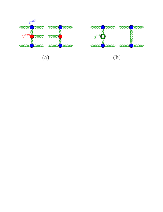
Figure 1: (a) The red blob along the gluon ladder represents the central–emission vertex within the tree-level five–gluon amplitude. (b) The pierced green blob represents the one–loop gluon Regge trajectory within the one–loop four–gluon amplitude. Momentum in the $s$ channel flows horizontally, and in the $t$ channel vertically.

The BFKL equation is an integral equation with an iterative structure. Its kernel is derived by singling out the emission of a gluon along the gluon ladder, fig. 1(a). The infrared divergences of the kernel, which result from integrating the gluon momentum over its phase space, are regulated by the infrared structure of the one-loop gluon Regge trajectory, fig. 1(b). It is possible to extend the BFKL equation to next-to-leading logarithmic (NLL) accuracy [16, 17, 18, 19], i.e. to resum the radiative corrections of ${\cal O}(\alpha_{\scriptscriptstyle S}(\alpha_{\scriptscriptstyle S}\ln(s/|t|))^{n})$, by considering the radiative corrections to the leading-order kernel. These corrections involve the emission of two gluons, or a $q\bar{q}$ pair, close in rapidity along the gluon ladder [20, 21, 22, 23, 24], fig. 2(a), and the one-loop corrections to the emission of a gluon along the ladder [25, 26, 27, 28, 29], fig. 2(b). The infrared divergences of the next-to-leading-order (NLO) kernel, which result from integrating the momenta of the partons emitted along the gluon ladder over their phase space, are regulated by the infrared structure of the two-loop gluon Regge trajectory, fig. 2(c).

Underpinning the BFKL equation at NLL accuracy is the fact that gluon Reggeization holds at that accuracy [30, 31]. Gluon Reggeization breaks down beyond NLL accuracy, because at next-to-next-to-leading logarithmic (NNLL) accuracy three-Reggeized-gluon exchanges appear [32, 33, 34, 35, 36, 37, 38, 39, 40, 41, 42]. The issue of whether a single-Reggeized-gluon exchange can be isolated and iterated through a BFKL kernel at NNLL accuracy remains to be understood; see sec. 2.9.

In the last decade, the study of the multi-Regge limit has deepened after the realization that it is a powerful kinematic constraint for amplitudes in QCD [43, 41, 44] and in the maximally supersymmetric gauge theory, ${\cal N}=4$ super-Yang-Mills theory (SYM) [45, 46, 47, 48, 49, 50, 51, 52, 53], and that in the Regge limit amplitudes in planar ${\cal N}=4$ SYM [54, 55, 56, 57], and amplitudes [58] and cross sections [59, 60] in QCD are endowed with a rich mathematical structure. Although we will not be able to cover them adequately in this review, effective field theory methods have been brought to bear on the Regge limit, including the role of Glauber gluons and quarks [61, 62]; they promise to lead to further progress on the systematic understanding of this limit in the future.

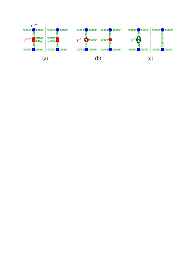
Figure 2: (a) The red blob along the gluon ladder represents the two-gluon central-emission vertex within the tree six-gluon amplitude. (b) The pierced red blob represents the one-loop central-emission vertex within the one-loop five–gluon amplitude. (c) The twice pierced green blob represents the two-loop gluon Regge trajectory within the two-loop four–gluon amplitude.

The multi-Regge limit has been studied extensively in ${\cal N}=4$ SYM, particularly in the limit of a large number of colors, $N_{c}\to\infty$, where planar Feynman diagrams dominate. In this introduction, we provide a review of some of these developments, prior to going into more detail on many of the topics in sec. 3.

In the planar limit, scattering amplitudes all have a definite cyclic color ordering, with distinct color lines in the fundamental ${\bf N_{c}}$ representation of $SU(N_{c})$ flowing along each edge. The color quantum numbers of a Reggeized object exchanged in a given channel, bounded by two oppositely-oriented edges, are ${\bf N_{c}}\otimes{\bf\overline{N}_{c}}={\bf(N_{c}^{2}-1)}\oplus{\bf 1}$, but the singlet contribution is suppressed by a factor of $1/N_{c}^{2}$. Hence the BFKL ladder studied in planar ${\cal N}=4$ SYM is for the adjoint representation, whereas QCD BFKL evolution is usually studied at the cross section level for the singlet channel. The richness of $n$-gluon scattering amplitudes in planar ${\cal N}=4$ SYM begins at $n=6$, due to an additional dual conformal symmetry present in the theory [63, 64, 65, 66, 67, 68, 69, 70, 71]. Because of this symmetry, the four- and five-gluon amplitudes are completely constrained kinematically to be given by the Bern-Dixon-Smirnov (BDS) ansatz [72], essentially the exponential of the one-loop amplitude, because it solves an anomalous dual conformal Ward identity [68].

Starting at $n=6$, the Ward identity allows for non-trivial functions of the kinematics, which depend on $3n-15$ dual conformal cross ratios. The first concrete indication that the BDS ansatz had to be modified at $n=6$ and at two loops came from multi-Regge kinematics (MRK), where it was shown that the ansatz violates Regge factorization for both $2\to 4$ and $3\to 3$ scattering in appropriate channels [73, 74]. Soon thereafter, the all-orders factorized structure for $2\to 4$ scattering in MRK was presented for the maximally-helicity-violating (MHV) configuration in terms of an inverse Fourier-Mellin (FM) transform of the exponentiated BFKL eigenvalue in the adjoint representation, multiplied by the product of impact factors for the top and bottom of the Reggeized ladder [75, 76]. The case of $3\to 3$ scattering was described in ref. [77]; although closely related to the $2\to 4$ case, it is slightly simpler because the Regge cut contribution in MRK is purely imaginary. The case of next-to-MHV (NMHV) helicities was analyzed at leading logarithms in ref. [78], and the all-orders factorized structure was described in refs. [55, 49].

The full power of integrability in planar ${\cal N}=4$ SYM was first brought to bear on the six-point MRK limit [55] by performing an intricate analytic continuation from the pentagon operator product expansion (POPE), or flux tube, representation of the near-collinear limit [79]. All-orders predictions were obtained for the adjoint BFKL eigenvalue and the impact factor, or in other words for all subleading logarithms at leading power in MRK, for both MHV and NMHV six-point amplitudes [55].

At each perturbative order, the inverse FM sum can be computed, and compared to the multi-Regge limit of amplitudes constructed in general kinematics. At two loops, the analytic form of the six-point MHV amplitude was found by explicit computation of a Wilson loop representation of the amplitude [45, 46], which was simplified down to just a few lines using the symbol associated with polylogarithmic functions [80]. The three- and four-loop MHV and two-, three- and four-loop NMHV amplitudes were bootstrapped using hexagon functions with the correct branch cuts, as well as boundary information from the near-collinear limit [47, 81, 82, 48, 83, 84]. The introduction of constraints on the function space from (extended) Steinmann relations has made it possible to push as far as seven loops [51, 52, 85]. In some cases the multi-Regge limit has been used to constrain the bootstrap ansatz; however, the information used is self-consistent, in the sense that it only requires loop orders in the BFKL eigenvalue and the impact factor that are already determined by the amplitude at the previous loop order. See Chapter 5 [86] of the SAGEX Review [87] for more details about the amplitude bootstrap.

In order to compare the perturbative results to the predictions from the inverse FM transform, it is helpful to realize that the six-point results can always be expressed [54] in terms of real analytic, or single-valued, harmonic polylogarithms (SVHPLs) for a single complex variable [88]. At higher points, multiple-variable SVHPLs appear, which are real analytic functions on the moduli space of Riemann spheres with marked points or punctures [56, 89]. Once the inverse FM transform is known for various building blocks in the FM representation, they can be combined using a convolution theorem [56]. The inverse FM transform can often be performed by brute force, by doing it as a truncated series expansion and matching the result to the series expansion of a general linear combination of SVHPLs of the appropriate weight [54]. Other algorithms are given in refs. [90, 91]. Using such methods, the six-point MRK limit predicted by ref. [55] has been verified through seven loops for both MHV and NMHV helicity configurations [52, 92].

Multi-Regge limits of planar ${\cal N}=4$ SYM amplitudes with more than six external legs have also received great attention, starting with $2\to 5$ scattering at leading logarithmic accuracy [93, 94, 95]. Besides the same impact factors and BFKL eigenvalue appearing in the six-point case, a new ${\cal N}=4$ ingredient, the central emission vertex (or Lipatov vertex), first appears for $n=7$ in the so-called “long” Regge cut configuration. The factorized structure beyond leading logarithms was described and the central emission vertex was obtained at next-to-leading order in ref. [96]. Based on higher-order perturbative data, and the general structure of the near-collinear limit, a proposal for the all-orders form of the central emission vertex was presented, and its perturbative predictions were checked at the symbol level through four loops for the MHV configuration [57], relying on the amplitudes bootstrapped in refs. [97, 98, 99]. Recently the proposal was checked through four loops at full function level for both MHV and NMHV seven-point amplitudes [100], making use of the zeta-valued constants fixed in ref. [101].

Beyond seven points, it is possible that no new ingredients are required for amplitudes in the long Regge cut configuration. This is the case at two loops, at least at the level of the symbol of the MHV $n$-point amplitude, which has been computed in generic kinematics [102], and studied in MRK [103, 104, 57]. However, as discussed further in the conclusions, for amplitudes in other cut configurations there still may be more to learn from double and higher discontinuities at two loops [105] and beyond [106].

At strong coupling, scattering amplitudes in planar ${\cal N}=4$ SYM are given in terms of the area of a minimal surface in five-dimensional anti-de Sitter space that is bounded by a polygon composed of light-like edges [65]. The minimal area problem is integrable and can be solved using a thermodynamic Bethe ansatz or $Y$-system [107, 108, 109]. These systems have been solved in multi-Regge limits [110, 111, 112, 113, 114, 115, 116], shedding light on the strong-coupling behavior, which at six-points must be consistent with the strong coupling limit of the all-orders results [55].

The remainder of this review is organized as follows. In sec. 2, we consider the multi-Regge limit of QCD amplitudes, the BFKL equation, its solution and the function space which describes it, at LL and at NLL accuracy. At the end of the section, we comment briefly on ongoing work beyond NLL accuracy. In sec. 3, we analyze the multi-Regge limit of amplitudes with six and seven points in planar ${\cal N}=4$ SYM. We describe the conformal cross ratios, the symbol alphabet, the function space, and the all-orders formulae which are supposed to hold for amplitudes at six and more points. In sec. 4, we draw our conclusions and briefly discuss the integrability picture of amplitudes in ${\cal N}=4$ SYM in the large $N_{c}$ limit.

2 The multi-Regge limit of QCD amplitudes

In the Regge limit, $s\gg|t|$, $2\to 2$ scattering amplitudes in QCD are dominated by gluon exchange in the $t$ channel. Contributions which do not feature gluon exchange in the $t$ channel are power suppressed in $t/s$. At tree level we can write the $2\to 2$ amplitudes in a factorized way. For example, the tree amplitude for gluon-gluon scattering $g_{1}\,g_{2}\to g_{3}\,g_{4}$ in the helicity basis may be written as [11, 13],

$${\cal M}^{(0)}_{4g}=\left[g_{\scriptscriptstyle S}(F^{a_{3}})_{a_{2}c}\,C^{g(0)}(p_{2}^{\nu_{2}},p_{3}^{\nu_{3}}))\right]{s\over t}\left[g_{\scriptscriptstyle S}(F^{a_{4}})_{a_{1}c}\,C^{g(0)}(p_{1}^{\nu_{1}},p_{4}^{\nu_{4}})\right]\,,$$ (1)

with momenta $p_{2}$ in the $+$ light-cone direction and $p_{1}$ in the $-$ light-cone direction, as shown in fig. 3. We use light-cone coordinates adapted to the incoming beam directions, $p^{\pm}=p_{0}\pm p_{z}$, and complexified transverse momenta $p_{\perp}=p_{x}+ip_{y}$, $p^{*}_{\perp}=p_{x}-ip_{y}$. Hence a momentum vector $p_{i}^{\mu}=(p_{i}^{+},p_{i}^{-},p_{i\perp})$ has Lorentz norm $p_{i}^{2}=p_{i}^{+}p_{i}^{-}-|p_{i\perp}|^{2}$, and $2p_{i}\cdot p_{j}=p_{i}^{+}p_{j}^{-}+p_{i}^{-}p_{j}^{+}-p_{i\perp}p_{j\perp}^{*}-p_{i\perp}^{*}p_{j\perp}$. In general, we denote external momenta by $p_{i}$ (occasionally $k_{i}$) and reserve $q_{i}$ for $t$-channel momentum exchanges between factorized emissions. In the present four-point case, we define $s=(p_{1}+p_{2})^{2}$, $q=p_{2}+p_{3}$, $t=q^{2}\simeq-|q_{\perp}|^{2}$, The superscripts $\nu_{i}$ label the helicities. The adjoint generators of the gauge group are the structure constants, $(F^{c})_{ab}=i\sqrt{2}f^{acb}$. It is apparent from the color coefficient $(F^{a_{3}})_{a_{2}c}(F^{a_{4}})_{a_{1}c}$ in eq. (1) that only the antisymmetric octet ${\bf 8}_{a}$ is exchanged in the $t$ channel.

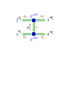
Figure 3: Amplitude for gluon-gluon scattering in the Regge limit. Momenta and helicities are labeled in black, color in red. The blue blobs represent the impact factors. The helicity labelling stresses that, at tree level and at leading power in $t/s$, helicity is conserved along the horizontal $s$-channel direction.

Because the four-gluon amplitude is a MHV amplitude, eq. (1) describes $\binom{4}{2}=6$ helicity configurations. However, at tree level and at leading power in $t/s$, helicity is conserved along the $s$-channel direction shown in fig. 3, or in our all-outgoing helicity convention,

$$C^{g}(p_{2}^{\nu_{2}},p_{3}^{\nu_{3}})\ \propto\ \delta^{\nu_{2},-\nu_{3}}.$$ (2)

Thus in eq. (1) four helicity configurations are leading, two for each tree-level impact factor, $g^{*}\,g\rightarrow g$, with $g^{*}$ an off-shell gluon [117],

$$C^{g(0)}(p_{2}^{\ominus},p_{3}^{\oplus})=1\,,\qquad C^{g(0)}(p_{1}^{\ominus},p_{4}^{\oplus})={p_{4\perp}^{*}\over p_{4\perp}}\,,$$ (3)

with complex transverse coordinates $p_{\perp}=p^{x}+ip^{y}$. At this order, the impact factors are just overall phases, and they transform under parity into their complex conjugates,

$$[C^{g}(p_{i}^{\nu},p_{j}^{\nu^{\prime}})]^{*}=C^{g}(p_{i}^{-\nu},p_{j}^{-\nu^{\prime}})\,.$$ (4)

The helicity-flip impact factor $C^{g(0)}(p_{i}^{\oplus},p_{j}^{\oplus})$ and its parity conjugate $C^{g(0)}(p_{i}^{\ominus},p_{j}^{\ominus})$ are power suppressed in $t/s$. However, helicity flip terms along the $s$-channel direction, and thus helicity–violating impact factors, do occur at one loop [25, 118, 119].

The tree amplitudes for quark-gluon or quark-quark scattering have the same form as eq. (1), up to replacing one or both gluon impact factors $C^{g(0)}$ in eq. (3) with quark impact factors $C^{q(0)}$, and the color factors $(F^{c})_{ab}$ in the adjoint representation with the color factors $T^{c}_{ij}$ in the fundamental representation of $SU(3)$, which we normalize as $\Tr(T^{a}T^{b})=T_{F}\delta^{ab}$, with $T_{F}=1$. So in the Regge limit, the $2\to 2$ scattering amplitudes factorize into gluon or quark impact factors and a gluon propagator in the $t$ channel, and are uniquely determined by them.

The loop corrections to an amplitude feature poles and branch cuts, which are dictated by the analytic structure and constrained by the symmetries of the amplitude. In the Regge limit $s\simeq-u\gg-t$, $2\to 2$ scattering amplitudes are symmetric under $s\leftrightarrow u$ crossing. Thus we may consider amplitude combinations whose kinematic and color coefficients have a definite signature under $s\leftrightarrow u$ crossing,

$${\cal M}_{4}^{(\pm)}(s,t)=\frac{{\cal M}_{4}(s,t)\pm{\cal M}_{4}(u,t)}{2}\,,$$ (5)

with $u=-s-t\simeq-s$, such that ${\cal M}_{4}^{(-)}(s,t)$ (${\cal M}_{4}^{(+)}(s,t)$) has kinematic and color coefficients which are both odd (even) under $s\leftrightarrow u$ crossing. Furthermore, higher-order contributions to $gg\rightarrow gg$ scattering in general involve additional color structures, as dictated by the decomposition of the product ${\bf 8}_{a}\otimes{\bf 8}_{a}$ into irreducible representations,

$${\bf 8}_{a}\otimes{\bf 8}_{a}\,=\,\{{\bf 1}\oplus{\bf 8}_{s}\oplus{\bf 27}\}\oplus[{\bf 8}_{a}\oplus{\bf 10}\oplus\overline{{\bf 10}}]\ \,,$$ (6)

where in curly (square) brackets are the representations which are even (odd) under $s\leftrightarrow u$ crossing.

2.1 The Regge limit at leading logarithmic accuracy

When loop corrections to the tree amplitude (1) are considered, it is found that at leading logarithmic (LL) accuracy in $\ln(s/|t|)$, the four-gluon amplitude is given to all orders in $\alpha_{\scriptscriptstyle S}$ by [11, 13]

$$\left.{\cal M}_{4g}\right|_{LL}=\left[g_{\scriptscriptstyle S}(F^{a_{3}})_{a_{2}c}\,C^{g(0)}(p_{2}^{\nu_{2}},p_{3}^{\nu_{3}}))\right]{s\over t}\left({s\over\tau}\right)^{\alpha(t)}\,\left[g_{\scriptscriptstyle S}(F^{a_{4}})_{a_{1}c}\,C^{g(0)}(p_{1}^{\nu_{1}},p_{4}^{\nu_{4}})\right]\,,$$ (7)

where $\tau>0$ is a Regge factorization scale, which is of order of $t$, although the precise definition of $\tau$ is immaterial for four-point amplitudes or to LL accuracy, where one can suitably fix $\tau=-t$. In eq. (7), $\alpha(t)$ is called the Regge trajectory. It is given by an integral over the loop transverse momentum,

$$\alpha(t)=\alpha_{\scriptscriptstyle S}\,C_{A}\,t\int{d^{2}k_{\perp}\over(2\pi)^{2}}\,{1\over k_{\perp}^{2}(q-k)_{\perp}^{2}}\,,$$ (8)

with $\alpha_{\scriptscriptstyle S}=g_{\scriptscriptstyle S}^{2}/(4\pi)$ and $C_{A}=N_{c}$ the number of colors. Regulating the integral in $d=4-2\epsilon$ dimensions, one obtains

$$\alpha(t)=\frac{N_{c}\alpha_{\scriptscriptstyle S}}{4\pi}\alpha^{(1)}(t)\,,\qquad{\rm with}\qquad\alpha^{(1)}(t)={\gamma_{K}^{(1)}\over 4\epsilon}\left(\mu^{2}\over-t\right)^{\epsilon}\kappa_{\Gamma}\,,$$ (9)

with

$$\kappa_{\Gamma}=(4\pi)^{\epsilon}\,{\Gamma(1+\epsilon)\,\Gamma^{2}(1-\epsilon)\over\Gamma(1-2\epsilon)}\,,$$ (10)

and where $\gamma_{K}^{(1)}$ is the one-loop coefficient of the cusp anomalous dimension [120, 121],

$$\gamma_{K}(\alpha_{\scriptscriptstyle S})=\sum_{\ell=1}^{\infty}\gamma_{K}^{(\ell)}\left(\frac{N_{c}\alpha_{\scriptscriptstyle S}}{4\pi}\right)^{\ell}\,,\quad{\rm with}\quad\gamma_{K}^{(1)}=8\,.$$ (11)

Although no renormalization occurs at LL accuracy, in eq. (9) the renormalization scale $\mu$ appears and provides a scaling dimension. Its presence is understood henceforth.

The prominent features of eq. (7) are that at LL accuracy the amplitude (7) is still real, the antisymmetric octet ${\bf 8}_{a}$ is still the only color representation exchanged in the $t$ channel,

$$\left.{\cal M}_{4g}\right|_{LL}=\left.{\cal M}^{(-)[8_{a}]}_{4g}\right|_{LL}\,,\qquad\qquad\left.{\cal M}^{(+)}_{4g}\right|_{LL}=0\,,$$ (12)

and the one-loop result (9) exponentiates. The exponentiation of $\ln(s/|t|)$ in the one-loop result, which effectively dresses the gluon propagator as

$$\frac{1}{t}\to\frac{1}{t}\left({s\over\tau}\right)^{\alpha(t)}\,,$$ (13)

is called gluon Reggeization, and we say that in the Regge limit the four-gluon amplitude (7) features the exchange in the $t$ channel of one Reggeized gluon.

Because of eq. (7), factorization holds at LL accuracy just like at tree level, i.e. the amplitudes for quark-gluon or quark-quark scattering at LL accuracy have the same form as eq. (7), up to replacing one or both color and impact factors for gluons with the ones for quarks.

2.2 The Multi-Regge limit

The Regge limit of the $2\to 2$ amplitudes in eq. (1) is characterized by strong orderings in the light-cone momenta of the two final-state gluons,

$$p_{3}^{+}\gg p_{4}^{+}\,,\qquad p_{3}^{-}\ll p_{4}^{-}\,,$$ (14)

where the second strong ordering is equivalent to the first because of the mass-shell conditions $p_{i}^{+}p_{i}^{-}=|p_{i\perp}|^{2}$, with $i=3,4$, and of transverse momentum conservation, $p_{3\perp}+p_{4\perp}=0$. Since for a light-like momentum, $p^{\pm}=|p_{\perp}|e^{\pm y}$, where $y$ is the rapidity, eq. (14) is equivalent to a strong ordering of the rapidities of the final-state gluons.

Next we consider $2\to 3$ amplitudes with momenta $p_{1}\,p_{2}\to p_{3}\,p_{4}\,p_{5}$. Here the Regge limit is realized by the two kinematic limits,

$$p_{3}^{+}\gg p_{4}^{+}\simeq p_{5}^{+}\quad{\rm or}\quad p_{3}^{+}\simeq p_{4}^{+}\gg p_{5}^{+}\,,\qquad{\rm with}\qquad|p_{3\perp}|\simeq|p_{4\perp}|\simeq|p_{5\perp}|\,.$$ (15)

The two kinematics of eq. (15) are termed next-to-multi-Regge kinematics (NMRK). They have an overlap in the kinematic region characterized by a strong ordering in the light-cone momenta of all three final-state gluons,

$$p_{3}^{+}\gg p_{4}^{+}\gg p_{5}^{+}\,,\qquad{\rm with}\qquad|p_{3\perp}|\simeq|p_{4\perp}|\simeq|p_{5\perp}|\,,$$ (16)

which is called multi-Regge kinematics (MRK). In MRK, the tree amplitude for five-gluon scattering $g_{1}\,g_{2}\to g_{3}\,g_{4}\,g_{5}$ takes the factorized ladder form,

$${\cal M}^{(0)}_{5g} = s\left[g_{\scriptscriptstyle S}(F^{a_{3}})_{a_{2}c_{1}}\,C^{g(0)}(p_{2}^{\nu_{2}},p_{3}^{\nu_{3}}))\right]\,{1\over t_{1}}$$

$$\times \left[g_{\scriptscriptstyle S}(F^{a_{4}})_{c_{1}c_{2}}\,V^{g(0)}(q_{1},p^{\nu_{4}}_{4},q_{2})\right]\,{1\over t_{2}}\,\left[g_{\scriptscriptstyle S}(F^{a_{5}})_{a_{1}c_{2}}\,C^{g(0)}(p_{1}^{\nu_{1}},p_{5}^{\nu_{5}})\right]\,.$$

with $q_{1}=p_{2}+p_{3}$, $q_{2}=q_{1}+p_{4}$, and $t_{i}=q_{i}^{2}\simeq-q_{i\perp}q_{i\perp}^{\ast}$, with $i=1,2$, where the impact factors are given in eq. (3). The emission of a gluon along the gluon ladder is governed by the central-emission vertex (CEV) [11, 122],

$$V^{g(0)}(q_{1},p^{\oplus}_{4},q_{2})=\frac{q_{1\perp}^{\ast}q_{2\perp}}{p_{4\perp}}\,.$$ (18)

Note that while eq. (2.2) displays soft divergences in the limit that gluon $p_{4}\to 0$, collinear divergences are screened by the MRK, eq. (16), which prevents the invariant mass of any two partons from becoming arbitrarily small.

2.3 The BFKL equation at LL accuracy

The ladder form of eq. (2.2) can be iterated to provide the tree amplitude for $n$-gluon scattering in MRK,

$$p_{3}^{+}\gg p_{4}^{+}\gg\ldots\gg p_{n}^{+}\,,$$ (19)

where a requirement on the transverse momenta to be all of the same size is understood, by adding $n-5$ central-emission vertices along the ladder of amplitude (2.2). The ensuing tree-level $n$-gluon amplitude, with $n-4$ central-emission vertices and $n-3$ gluon propagators, is uplifted to all orders in $\alpha_{\scriptscriptstyle S}$, at LL accuracy in $\ln(s/|t|)$, by dressing each of the gluon propagators as in eq. (13). Just like the four-gluon amplitude (7) in the Regge limit, the $n$-gluon amplitude in MRK at LL accuracy is characterized by the exchange of one Reggeized gluon, which is termed the Reggeon.

The central-emission vertex (18), fig. 1(a), and the gluon Reggeization (13), fig. 1(b), constitute the building blocks of an iterative structure, which is captured by the BFKL equation [12, 13, 14, 15], which sums the terms of ${\cal O}(\alpha_{\scriptscriptstyle S}^{n}\ln^{n}(s/|t|))$ and describes the evolution of a gluon ladder in transverse momentum and in rapidity. In the BFKL equation, real emissions as well as virtual ones are included. In order to match the LL accuracy of the virtual corrections (7), amplitudes with five or more gluons are taken in MRK (16), as in eq. (2.2). The MRK rationale is that each gluon emitted along the ladder requires a factor of $\alpha_{\scriptscriptstyle S}$, and the integral over its rapidity yields a factor of $\ln(s/|t|)$, so that each emitted gluon contributes a factor of ${\cal O}(\alpha_{\scriptscriptstyle S}\ln(s/|t|))$.

We can display how the BFKL equation works by considering gluon-gluon scattering. In the Regge limit, at leading order in $\alpha_{\scriptscriptstyle S}$, i.e. ${\cal O}(\alpha_{\scriptscriptstyle S}^{2})$, the partonic cross section for gluon-gluon scattering $g_{1}\,g_{2}\to g_{3}\,g_{4}$ is [123]

$${d\hat{\sigma}_{gg}^{(0)}\over d^{2}p_{3\perp}d^{2}p_{4\perp}}\ =\ \biggl{[}{N_{c}\alpha_{\scriptscriptstyle S}\over|p_{3\perp}|^{2}}\biggr{]}\,{1\over 2}\delta^{(2)}(p_{3\perp}+p_{4\perp})\,\biggl{[}{N_{c}\alpha_{\scriptscriptstyle S}\over|p_{4\perp}|^{2}}\biggr{]}\,,$$ (20)

which is obtained by squaring amplitude (1) and integrating it over the phase space of the final-state gluons 3 and 4. The terms in square brackets are related to the square of the impact factors (3), which is just 1, multiplied by an overall factor. The real corrections in $\alpha_{\scriptscriptstyle S}$, i.e. ${\cal O}(\alpha_{\scriptscriptstyle S}^{3})$, are obtained by squaring the five-gluon amplitude (2.2), whose momenta we re-label as $p_{1}p_{2}\to p_{3}k_{1}p_{4}$, and integrating it over the phase space of the final-state gluons [124],

$${d\hat{\sigma}_{gg}^{(1r)}\over d^{2}p_{3\perp}d^{2}p_{4\perp}}\ =\ \biggl{[}{N_{c}\alpha_{\scriptscriptstyle S}\over|p_{3\perp}|^{2}}\biggr{]}\,\frac{N_{c}\alpha_{\scriptscriptstyle S}}{\pi^{2}}\int\frac{d^{2}k_{1\perp}dy_{k_{1}}}{k_{1\perp}^{2}}{1\over 2}\delta^{(2)}(p_{3\perp}+k_{1\perp}+p_{4\perp})\,\biggl{[}{N_{c}\alpha_{\scriptscriptstyle S}\over|p_{4\perp}|^{2}}\biggr{]}\ ,$$ (21)

where the superscript (1r) on the left-hand-side stands for real radiation of the first loop order. In eq. (21), $y_{k_{1}}$ is integrated over the range $\Delta y=y_{3}-y_{4}=\ln(s_{12}/|p_{3\perp}||p_{4\perp}|)$. The integral over $k_{1\perp}$ yields a logarithmic soft singularity, which is regulated by including the virtual corrections, eqs. (7) and (8). The finite remainder is a term of ${\cal O}(\alpha_{\scriptscriptstyle S}\Delta y)$.

The subsequent orders in $\alpha_{\scriptscriptstyle S}$ each yield an integral over transverse momentum with a weight $\frac{N_{c}\alpha_{\scriptscriptstyle S}}{\pi^{2}}\int\frac{{\rm d}^{2}k_{i\perp}}{k_{i\perp}^{2}}$, and an integral over rapidity bounded as in eq. (19), which for the ${\cal O}(\alpha_{\scriptscriptstyle S}^{n+2})$ corrections yield a factor of $\frac{(\Delta y)^{n}}{n!}$. Including all the orders of ${\cal O}(\alpha_{\scriptscriptstyle S}\Delta y)$, the gluon-gluon initiated cross section in the Regge limit can be written as [125, 126, 127]

$${d\hat{\sigma}_{gg}\over d^{2}p_{3\perp}d^{2}p_{4\perp}}\ =\ \biggl{[}{N_{c}\alpha_{\scriptscriptstyle S}\over|p_{3\perp}|^{2}}\biggr{]}\,f(q_{1\perp},q_{2\perp},\Delta y)\,\biggl{[}{N_{c}\alpha_{\scriptscriptstyle S}\over|p_{4\perp}|^{2}}\biggr{]}\ ,$$ (22)

where, as in eq. (2.2), $q_{1\perp}=p_{3\perp}$ and $q_{2\perp}=-p_{4\perp}$. $f(q_{1\perp},q_{2\perp},\Delta y)$ is the solution of the BFKL equation for evolution in rapidity,

$$\frac{\partial}{\partial\Delta y}f(q_{1\perp},q_{2\perp},\Delta y)\ =\ \left({\cal K}\star f\right)(q_{1\perp},q_{2\perp},\Delta y)\,,$$ (23)

which can be given an explicit iterative form by writing it as [128]

$$f(q_{1\perp},q_{2\perp},\Delta y) = {1\over 2}\delta^{(2)}(p_{3\perp}+p_{4\perp})$$ (24)

$$+ \Delta y\,{\cal K}\left[{1\over 2}\delta^{(2)}(p_{3\perp}+p_{4\perp})\right]$$

$$+ \frac{(\Delta y)^{2}}{2}{\cal K}\left[{\cal K}\left[{1\over 2}\delta^{(2)}(p_{3\perp}+p_{4\perp})\right]\right]$$

$$+ \frac{(\Delta y)^{2}}{3!}{\cal K}\left[{\cal K}\left[{\cal K}\left[{1\over 2}\delta^{(2)}(p_{3\perp}+p_{4\perp})\right]\right]\right]$$

$$+ \ldots\,.$$

The integral operator ${\cal K}$ is a convolution,

$${\cal K}\left[f(q_{1\perp},q_{2\perp})\right]=\left({\cal K}\star f\right)(q_{1\perp},q_{2\perp})=\int d^{2}k_{\perp}K(q_{1\perp},k_{\perp})f(k_{\perp},q_{2\perp})\,,$$ (25)

with

$$\left({\cal K}\star f\right)(q_{1\perp},q_{2\perp})$$

$$\qquad=\frac{N_{c}\alpha_{\scriptscriptstyle S}}{\pi^{2}}\int d^{2}k_{\perp}\frac{1}{|q_{1\perp}-k_{\perp}|^{2}}\left(f(k_{\perp},q_{2\perp})-{|q_{1\perp}|^{2}\over|k_{\perp}|^{2}+|q_{1\perp}-k_{\perp}|^{2}}f(q_{1\perp},q_{2\perp})\right),$$ (26)

where the first term corresponds to the emission of a gluon along the ladder, eqs. (18) and (21), and the second term to the virtual corrections, eqs. (7) and (8) (after partial fractioning and a change of integration variable).

The kernel $K$ is obtained by generalizing eq. (2.2) to $n$-gluon scattering in MRK and by Reggeizing, like in eq. (13), each of the $(n-3)$ ensuing gluon propagators [12, 13, 14] in order to obtain the $n$-gluon amplitude at LL accuracy. This is then squared (the square of the CEV (18) will yield the first term of eq. (26)) and integrated over the phase space of the $(n-2)$ outgoing gluons. The rapidities are integrated over, while the $(n-2)$ integrals over transverse momentum can be written as a recursive relation through the integral operator (25) [123]. Using the fact that the square of the CEV (18) is regular as $q_{2\perp}\to\infty$ and vanishes as $q_{2\perp}\to 0$, it is possible to show [123] that eq. (26) and thus the solution (24) of the BFKL equation are regular in the ultraviolet and in the infrared regimes, respectively.

The solution (24) of the BFKL equation is amenable to a Monte Carlo implementation of the gluon ladder [129, 130, 131]. The resummed form of the solution [14, 15] is obtained by transforming it to moment space,

$$f(q_{1\perp},q_{2\perp},\Delta y)\ =\ \int{d\omega\over 2\pi i}\,e^{\omega\Delta y}\,f_{\omega}(q_{1\perp},q_{2\perp})$$ (27)

such that we can write the BFKL equation as

$$\omega\,f_{\omega}(q_{1\perp},q_{2\perp})\,={1\over 2}\,\delta^{(2)}(q_{1\perp}-q_{2\perp})\,+\left({\cal K}\star f_{\omega}\right)(q_{1\perp},q_{2\perp})\,,$$ (28)

with the kernel $K$ as in eq. (26). The BFKL equation is solved by finding a set of eigenfunctions $\Phi_{\nu n}(q)$ of the integral operator ${\cal K}$,

$$\left({\cal K}\star\Phi_{\nu n}\right)(q_{\perp})=\omega_{\nu n}\Phi_{\nu n}(q_{\perp})\,,$$ (29)

where $\nu$ is a real number, $n$ is an integer, and $\omega_{\nu n}$ is the BFKL eigenvalue [15]. In a conformally-invariant theory, the eigenfunctions $\Phi_{\nu n}(q)$ are fixed by conformal symmetry [132]. They coincide with the eigenfunctions $\varphi_{\nu n}(q)$ of QCD at LL accuracy,

$$\Phi_{\nu n}(q)\equiv\varphi_{\nu n}(q)={1\over 2\pi}\,(q^{2})^{-1/2+i\nu}\,e^{in\theta}\,,$$ (30)

where $\theta$ is the azimuthal angle of $q$, and they satisfy the completeness relation,

$$\sum_{n=-\infty}^{+\infty}\int_{-\infty}^{+\infty}d\nu\,\Phi_{\nu n}(q)\,\Phi_{\nu n}^{\ast}({q^{\prime}})={1\over 2}\,\delta^{(2)}(q-q^{\prime})=\delta\left(q^{2}-{q^{\prime}}^{2}\right)\,\delta(\theta-\theta^{\prime})\,.$$ (31)

In terms of the eigenfunctions (30) and the eigenvalue in eq. (29), the solution to the BFKL equation (28) can be written as

$$f_{\omega}(q_{1},q_{2})\,=\sum_{n=-\infty}^{+\infty}\int_{-\infty}^{+\infty}d\nu\,{1\over\omega-\omega_{\nu n}}\,\Phi_{\nu n}(q_{1})\,\Phi_{\nu n}^{\ast}(q_{2})\,.$$ (32)

In fact, we can apply the integral operator to eq. (32),

$$({\cal K}\star f_{\omega})(q_{1},q_{2})=\sum_{n=-\infty}^{+\infty}\int_{-\infty}^{+\infty}d\nu\,{1\over\omega-\omega_{\nu n}}\,({\cal K}\star\Phi_{\nu n})(q_{1})\,\Phi_{\nu n}^{\ast}(q_{2})\,.$$ (33)

Then using eq. (29) and the completeness relation (31) in eq. (33), the BFKL equation (28) is identically satisfied.

Using eq. (27) on the solution (32) of the BFKL equation, we can write it as

$$f(q_{1\perp},q_{2\perp},\Delta y)=\sum_{n=-\infty}^{\infty}\int_{-\infty}^{\infty}d\nu\,\Phi_{\nu n}(q_{1})\,\Phi^{\ast}_{\nu n}(q_{2})\,e^{\Delta y\,\omega_{\nu n}}\,,$$ (34)

which, using the eigenfunctions (30), becomes

$$f(q_{1\perp},q_{2\perp},\Delta y)={1\over(2\pi)^{2}\sqrt{|q_{1\perp}|^{2}|q_{2\perp}|^{2}}}\sum_{n=-\infty}^{\infty}e^{in\phi}\,\int_{-\infty}^{\infty}d\nu\,e^{\eta\,\chi_{\nu n}}\,\left(|q_{1\perp}|^{2}\over|q_{2\perp}|^{2}\right)^{i\nu}\,,$$ (35)

where $\phi$ is the angle between $q_{1\perp}$ and $q_{2\perp}$. The exponent in eq. (35) is given by $\eta\,\chi_{\nu n}=\Delta y\,\omega_{\nu n}$, with

$$\eta=\frac{N_{c}\alpha_{\scriptscriptstyle S}}{\pi}\Delta y\,,$$ (36)

where the BFKL eigenvalue is

$$\omega_{\nu n}=\frac{N_{c}\alpha_{\scriptscriptstyle S}}{\pi}\,\chi_{\nu n}\,,$$ (37)

In order to find the explicit form of the eigenvalue $\chi_{\nu n}$ in eq. (37), we replace the solution (32) with the eigenfunctions (30) into the homogeneous part of the BFKL equation (28), and we obtain

$$\chi_{\nu n} = 2\,{\rm Re}\int_{0}^{1}dx\,{x^{{|n|-1\over 2}+i\nu}\over 1-x}-2\int_{0}^{1}dx\,{1\over 1-x}$$ (38)

$$- \int_{0}^{1}dx\,{1\over x}\,+\,\int_{0}^{1}dx\,{1\over x\sqrt{1+4x^{2}}}\,+\,\int_{0}^{1}dx\,{1\over\sqrt{x^{2}+4}}\,,$$

with

$$x=\,\left\{\begin{array}[]{ll}q_{2}^{2}/q_{1}^{2}&\mbox{for $q_{2}^{2}<q_{1}^{2}$}\,,\\ q_{1}^{2}/q_{2}^{2}&\mbox{for $q_{2}^{2}>q_{1}^{2}$}\,.\end{array}\right.$$ (39)

The last three terms in eq. (38) cancel out, and the eigenvalue becomes

$$\chi_{\nu n}=-2\gamma_{E}-\psi\left(\frac{1}{2}+\frac{|n|}{2}+i\nu\right)-\psi\left(\frac{1}{2}+\frac{|n|}{2}-i\nu\right)\,,$$ (40)

where $\gamma_{E}=-\psi(1)$ is the Euler-Mascheroni constant and

$${d\ln{\Gamma(y)}\over dy}\,=\,\psi(y)\,=\,\int_{0}^{1}dx{x^{y-1}-1\over x-1}-\gamma_{E}\,$$ (41)

is the logarithmic derivative of the $\Gamma$ function.

Note that the kernel $K$ (26) is real and symmetric, so the integral operator ${\cal K}$ (25) is hermitian and its eigenvalue (37) is real. In addition, in eq. (37) there are no beta function terms, in accordance with the lack of collinear or ultraviolet divergences in the BFKL kernel. Accordingly, the BFKL eigenvalue at LL accuracy is the same in QCD and in ${\cal N}=4$ SYM. Finally, in the BFKL eigenvalue (37) there are only leading $N_{c}$ terms.

The solution (35) of the BFKL equation at LL accuracy can be expanded into a power series in $\eta$,

$$f(q_{1\bot},q_{2\bot},\Delta y)=\frac{1}{2}\delta^{(2)}(q_{1\bot}-q_{2\bot})+\frac{1}{2\pi\,\sqrt{|q_{1\perp}|^{2}|q_{2\perp}|^{2}}}\,\sum_{k=1}^{\infty}\eta^{k}\,f_{k}(w,w^{\ast})\,,$$ (42)

where $w$ is a complex variable,

$$w=\frac{p_{3\perp}}{p_{4\perp}}\,,$$ (43)

such that

$$|w|^{2}=\frac{|p_{3\bot}|^{2}}{|p_{4\bot}|^{2}}=\frac{|q_{1\bot}|^{2}}{|q_{2\bot}|^{2}}{\rm~{}~{}~{}~{}and~{}~{}~{}~{}}\left(\frac{w}{w^{\ast}}\right)^{1/2}=e^{-i\phi_{jj}}=-e^{i\phi}\,,$$ (44)

where $\phi_{jj}=\pi-\phi$ is the angle between $p_{3\perp}$ and $p_{4\perp}$. In eq. (42), the coefficients $f_{k}$ are given by the FM transform,

$$f_{k}(w,w^{\ast})={\cal F}[\chi_{\nu n}^{k}]=\frac{1}{k!}\sum_{n=-\infty}^{+\infty}(-1)^{n}\,\left(\frac{w}{w^{\ast}}\right)^{n/2}\int_{-\infty}^{+\infty}\frac{d\nu}{2\pi}\,|w|^{2i\nu}\,\chi_{\nu n}^{k}\,.$$ (45)

The coefficients $f_{k}$ are real-analytic functions of $w$, that is, they have a unique, well-defined value for every ratio of the magnitudes of the two jet transverse momenta and angle between them. Furthermore, eq. (45) is invariant under $n\leftrightarrow-n$ and $\nu\leftrightarrow-\nu$, which implies that the $f_{k}$ are invariant under conjugation and inversion of $w$,

$$f_{k}(w,w^{\ast})=f_{k}(w^{\ast},w)=f_{k}(1/w,1/w^{\ast})\,,$$ (46)

i.e. the coefficients $f_{k}$ are eigenfunctions under the action of the $\mathbb{Z}_{2}\times\mathbb{Z}_{2}$ symmetry generated by

$$(w,w^{\ast})\leftrightarrow(w^{\ast},w){\rm~{}~{}~{}~{}and~{}~{}~{}~{}}(w,w^{\ast})\leftrightarrow(1/w,1/w^{\ast})\,.$$ (47)

A special point in the $(w,w^{\ast})$ plane is at $w=w^{\ast}=-1$, which corresponds to the Born kinematics, where the two jets are back-to-back, with equal and opposite transverse momentum, $|p_{3\bot}|^{2}=|p_{4\bot}|^{2}$ and $\phi_{jj}=\pi$. Another special point is the origin, $w=w^{\ast}=0$, when one jet has much smaller transverse momentum than the other jet. The point at infinity is related to the origin by the inversion symmetry, while $w=w^{\ast}=-1$ is a fixed point of the $\mathbb{Z}_{2}\times\mathbb{Z}_{2}$ symmetry (47).

In analogy with the multi-Regge limit of the six-point MHV and NMHV amplitudes in ${\cal N}=4$ SYM theory [133], a generating function can be introduced such as to write the coefficients $f_{k}$ as [59]

$$f_{k}(w,w^{\ast})=\frac{|w|}{|1+w|^{2}}\,F_{k}(w,w^{\ast})\,,$$ (48)

where the pure transcendental functions $F_{k}$ are given in terms of SVHPLs. For example, the first few loop orders of the functions $F_{k}$ are

$$F_{1}(w,w^{\ast}) = 1\,,$$

$$F_{2}(w,w^{\ast}) = -{\cal L}_{1}-\frac{1}{2}{\cal L}_{0}\,,$$

$$F_{3}(w,w^{\ast}) = {\cal L}_{1,1}+\frac{1}{2}({\cal L}_{0,1}+{\cal L}_{1,0})+\frac{1}{6}{\cal L}_{0,0}\,.$$ (49)

In order to make contact with the SVHPLs ${\cal L}_{\vec{\omega}}(z,\bar{z})$ defined in sec. 3.2, eqs. (147)–(148), we note that the poles of the SVHPLs are at $z=0$ and 1, not $w=0$ and $-1$, so we will need to identify $(z,\bar{z})=(-w,-w^{\ast})$; thus in eq. (49) it is understood that ${\cal L}_{\vec{\omega}}\equiv{\cal L}_{\vec{\omega}}(-w,-w^{\ast})$. Finally, using the $\mathbb{Z}_{2}\times\mathbb{Z}_{2}$ symmetry (47), projections of the SVHPLs onto eigenstates under conjugation as well as under inversion can be defined [54].

Using the all-orders expression for the perturbative expansion of the BFKL solution (42) at LL accuracy, we can immediately write down the explicit expression for the gluon-gluon cross section (22) in the Regge limit to any loop order, in LL approximation. In particular, we can obtain explicit analytic expressions for the dijet cross section in the Regge limit at LL accuracy that are inclusive in the transverse momentum and exclusive in the azimuthal angle, or vice-versa, or inclusive in both. Accordingly, analytic expressions for the azimuthal-angle distribution and for the transverse-momentum distribution were obtained [59], as well for the case where both the transverse momenta (above a threshold $E_{\bot}$) and the azimuthal angle are integrated over, the so-called Mueller-Navelet dijet cross section [125],

$$\hat{\sigma}_{gg}=\frac{\pi(N_{c}\alpha_{\scriptscriptstyle S})^{2}}{2E_{\bot}^{2}}\,\sum_{k=0}^{\infty}f_{0,k}\,\eta^{k}\,,$$ (50)

for which the coefficients $f_{0,k}$ were computed analytically through the $13^{\rm th}$ order in terms of multiple zeta values [59]. As an example, we reproduce here the coefficient of the $13^{\rm th}$ order,

$$f_{0,13} = \frac{4513}{1890}\,\zeta_{5,3}\,\zeta_{5}+\frac{27248}{23625}\,\zeta_{5,3,3}\,\zeta_{2}-\frac{97003}{235200}\,\zeta_{5,5,3}+\frac{13411}{75600}\,\zeta_{7,3}\,\zeta_{3}$$ (51)

$$+ \frac{7997743}{12700800}\,\zeta_{7,3,3}-\frac{187318}{14175}\,\zeta_{4}\,\zeta_{3}^{3}-\frac{125056}{4725}\,\zeta_{2}\,\zeta_{5}\,\zeta_{3}^{2}-\frac{17411413}{302400}\,\zeta_{7}\,\zeta_{3}^{2}$$

$$- \frac{5724191}{100800}\,\zeta_{5}^{2}\,\zeta_{3}-\frac{1874972477}{2376000}\,\zeta_{10}\,\zeta_{3}-\frac{2418071698069}{2235340800}\,\zeta_{13}$$

$$- \frac{2379684877}{6048000}\,\zeta_{11}\,\zeta_{2}-\frac{297666465053}{523908000}\,\zeta_{6}\,\zeta_{7}-\frac{1770762319}{2494800}\,\zeta_{5}\,\zeta_{8}$$

$$- \frac{229717224973}{628689600}\,\zeta_{4}\,\zeta_{9}\,.$$

2.4 The Regge limit at NLL accuracy

At next-to-leading-logarithmic (NLL) accuracy, taking into account the $s\leftrightarrow u$ crossing symmetry (5), the exchange of one Reggeized gluon of eq. (7) generalizes to [25]

$${\cal M}^{(-)[8_{a}]}_{4g}$$

$$= \frac{1}{2}\left[g_{\scriptscriptstyle S}(F^{a_{3}})_{a_{2}c}\,C^{g}(p_{2}^{\nu_{2}},p_{3}^{\nu_{3}})\right]{s\over t}\left[\left({s\over\tau}\right)^{\alpha(t)}+\left({-s\over\tau}\right)^{\alpha(t)}\right]\,\left[g_{\scriptscriptstyle S}(F^{a_{4}})_{a_{1}c}\,C^{g}(p_{1}^{\nu_{1}},p_{4}^{\nu_{4}})\right]\,,$$

where the color and kinematic parts of the amplitude are each odd under $s\leftrightarrow u$ crossing, and where we expand in $\alpha_{\scriptscriptstyle S}$ the gluon Regge trajectory,

$$\alpha(t)=\frac{N_{c}\alpha_{\scriptscriptstyle S}}{4\pi}\alpha^{(1)}(t)+\left(\frac{N_{c}\alpha_{\scriptscriptstyle S}}{4\pi}\right)^{2}\alpha^{(2)}(t)+{\cal O}(\alpha_{\scriptscriptstyle S}^{3})\,,$$ (53)

with $\alpha^{(1)}(t)$ given in eq. (9), and where the (unrenormalized) two-loop coefficient, in the conventional dimensional regularization (CDR)/’t-Hooft-Veltman (HV) schemes, is [134, 135, 136, 137, 32]

$$\alpha^{(2)}(t)=\kappa_{\Gamma}^{2}\left(\mu^{2}\over-t\right)^{2\epsilon}\left(\frac{\beta_{0}}{\epsilon^{2}}+\frac{\gamma_{K}^{(2)}}{8\epsilon}+\frac{\gamma_{\wedge}^{(2)}}{2}+\zeta_{2}\beta_{0}\right)+{\cal O}(\epsilon)\,,$$ (54)

with $N_{f}$ the number of light quark flavors, $\beta_{0}$ the one-loop coefficient of the beta function,

$$\beta_{0}=\frac{11}{3}-\frac{2}{3}\frac{N_{f}}{N_{c}}\,,$$ (55)

$\gamma_{\wedge}^{(2)}$ the two-loop coefficient of the “wedge” anomalous dimension [138, 139] for Wilson lines in the adjoint representation, which starts at two loops,

$$\gamma_{\wedge}(\alpha_{\scriptscriptstyle S})=\sum_{\ell=2}^{\infty}\gamma_{\wedge}^{(\ell)}\left(\frac{N_{c}\alpha_{\scriptscriptstyle S}}{4\pi}\right)^{\ell},\quad{\rm with}\quad\gamma_{\wedge}^{(2)}={808\over 27}-4\zeta_{3}-{112\over 27}\,\frac{N_{f}}{N_{c}}-2\zeta_{2}\beta_{0}\,,$$ (56)

and $\gamma_{K}^{(2)}$ the two-loop coefficient [140, 141] of the cusp anomalous dimension (11),

$$\gamma_{K}^{(2)}=8\left(\frac{64}{9}+\frac{\delta_{R}}{3}-2\zeta_{2}\right)-\frac{80}{9}\frac{N_{f}}{N_{c}}\,,$$ (57)

where

$$\delta_{R}=\left\{\begin{array}[]{ll}1&\mbox{HV/CDR},\\ 0&\mbox{DR/FDH}.\end{array}\right.$$ (58)

$\delta_{R}$ is a regularization parameter, which labels the computation as done in CDR/HV schemes for $\delta_{R}=1$, or in the dimensional reduction (DR)/ four dimensional helicity (FDH) schemes for $\delta_{R}=0$.

In eq. (2.4), the helicity-conserving impact factor is expanded in $\alpha_{\scriptscriptstyle S}$ as

$$C^{g}(p_{i}^{\nu_{i}},p_{j}^{-\nu_{i}};\tau)=C^{g(0)}(p_{i}^{\nu_{i}},p_{j}^{-\nu_{i}})\left(1+\frac{N_{c}\alpha_{\scriptscriptstyle S}}{4\pi}c^{g(1)}(t;\tau)+{\cal O}(\alpha_{\scriptscriptstyle S}^{2})\right)\,,$$ (59)

where the one-loop coefficient $c^{g(1)}$ is real and independent of the helicity configuration. Its unrenormalized version is [25, 118, 142, 119, 29, 143]

$$c^{g(1)}(t,\tau) = \kappa_{\Gamma}\left({\mu^{2}\over-t}\right)^{\epsilon}\bigg{[}-\frac{\gamma_{K}^{(1)}}{4\epsilon^{2}}+\frac{\gamma_{g}^{(1)}}{\epsilon}+\frac{\beta_{0}}{2\epsilon}+\frac{\gamma_{K}^{(1)}}{8\epsilon}\ln\left(\frac{\tau}{-t}\right)-\frac{\gamma_{K}^{(2)}}{16}+2\zeta_{2}$$ (60)

$$\qquad\qquad\quad-\frac{1}{2}\left(\frac{\gamma_{\wedge}^{(2)}}{2}+\zeta_{2}\beta_{0}\right)\epsilon\bigg{]}+{\cal O}(\epsilon^{2})\,,$$

where $\gamma_{g}^{(1)}$ is the one-loop coefficient of the gluon collinear anomalous dimension,

$$\gamma_{g}(\alpha_{\scriptscriptstyle S})=\sum_{\ell=1}^{\infty}\gamma_{g}^{(\ell)}\left(\frac{N_{c}\alpha_{\scriptscriptstyle S}}{4\pi}\right)^{\ell}\,,\qquad{\rm with}\qquad\gamma_{g}^{(1)}=-\beta_{0}\,.$$ (61)

Eq. (60) is valid in the CDR/HV [25, 118, 119, 29] and DR/FDH [119, 29] schemes through ${\cal O}(\epsilon^{0})$, and in the HV scheme through ${\cal O}(\epsilon)$. Expressions to all orders in $\epsilon$ are known in the HV scheme [25, 118, 29]. Note that the two-loop trajectory (54) and the one-loop impact factor (60) are expressed in terms of anomalous dimensions which are characteristic of infrared factorization in the Regge limit [33, 34, 35, 36]. However, the connection [143] between the ${\cal O}(\epsilon^{0})$ term of the two-loop trajectory (54) and the ${\cal O}(\epsilon)$ term of the one-loop impact factor (60) is as yet unexplained.

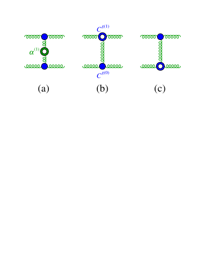
Figure 4: One-loop factorization of the four-gluon amplitude. (a) The one-loop gluon Regge trajectory is represented by the pierced green blob. (b) The one-loop gluon impact factor is represented by the pierced blue blob.

In addition, we may define a signature-symmetric logarithm,

$$L=\frac{1}{2}\left[\ln\left({s\over\tau}\right)+\ln\left({-s\over\tau}\right)\right]=\ln\left({s\over\tau}\right)-i\frac{\pi}{2}\,,$$ (62)

and write the four-gluon amplitude (2.4) as a double expansion in $\alpha_{\scriptscriptstyle S}$ and in $L$,

$${\cal M}^{(-)[8_{a}]}_{4g}={\cal M}^{(0)}_{4g}\left(1+\sum_{\ell=1}^{\infty}\left(\frac{N_{c}\alpha_{\scriptscriptstyle S}}{4\pi}\right)^{\ell}\sum_{i=0}^{\ell}M^{(-,\ell,i)[8_{a}]}_{4g}L^{i}\right)\,,$$ (63)

where $i=\ell$ yields the coefficients at LL accuracy, $i=\ell-1$ the coefficients at NLL accuracy, and in general $i=\ell-k$ the coefficients at $\mathrm{N^{k}LL}$ accuracy.

Beyond LL accuracy, in the gluon ladder the exchange of two or more Reggeized gluons may appear. Furthermore, all the color representations (6) exchanged in the $t$ channel may contribute. A similar expansion to eq. (63) can be given for the amplitudes ${\cal M}^{(+)}_{4g}$ whose kinematic and color parts are both even under $s\leftrightarrow u$ crossing. Using the logarithm (62), one can show that the coefficients $M^{(\mp,\ell,i)}_{4g}$ of the odd (even) amplitudes are real (imaginary) [38], and that the odd (even) amplitudes display gluon ladders with the $t$-channel exchange of an odd (even) number of Reggeized gluons.

However, at NLL accuracy, the real part of the amplitude is entirely given by the antisymmetric octet ${\bf 8}_{a}$ through eq. (2.4),

$${\rm Re}\left[{\cal M}_{4g}\right]_{NLL}={\rm Re}\left[{\cal M}^{(-)[8_{a}]}_{4g}\right]\,,$$ (64)

which, once eq. (2.4) is expanded at one and two loops reads,

$${\rm Re}\left[{\cal M}^{(1)}_{4g}\right]_{NLL} = \alpha^{(1)}(t)\ln\left(\frac{s}{\tau}\right)+2c^{g(1)}(t,\tau)\,,$$ (65)

$${\rm Re}\left[{\cal M}^{(2)}_{4g}\right]_{NLL} = \frac{1}{2}\left(\alpha^{(1)}(t)\right)^{2}\ln^{2}\left(\frac{s}{\tau}\right)+\left(\alpha^{(2)}(t)+2c^{g(1)}(t,\tau)\alpha^{(1)}(t)\right)\ln\left(\frac{s}{\tau}\right)\,.$$ (66)

Eq. (65) is the one-loop factorization of the gluon-gluon amplitude. The single-logarithmic term is the one-loop gluon Regge trajectory, fig. 4(a), which is LL accurate. The non-logarithmic terms are the one-loop impact factors, fig. 4(b, c), which are NLL accurate. Eq. (66) is the two-loop factorization of the gluon-gluon amplitude at NLL accuracy. The double-logarithmic term is the one-loop trajectory squared, fig. 5(a), which is LL accurate. The single-logarithmic terms are the two-loop gluon Regge trajectory, fig. 5(b), and the product of the one-loop trajectory times the one-loop impact factors, figs. 5(c, d). They are NLL accurate.

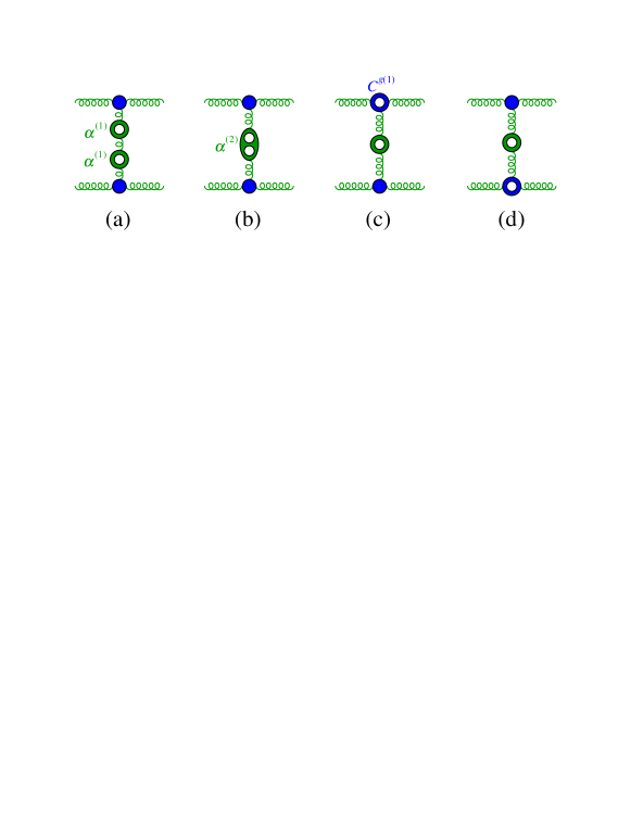
Figure 5: Two-loop factorization of the four-gluon amplitude at NLL accuracy. (a) The one-loop gluon Regge trajectory squared. (b) The two-loop gluon Regge trajectory is represented by the twice pierced green blob. (c, d) The product of the one-loop trajectory times the one-loop impact factor.

Beyond two loops, no more coefficients occur at NLL accuracy, i.e. the gluon-gluon scattering amplitude is uniquely determined by eq. (2.4), in terms of the two-loop Regge trajectory $\alpha^{(2)}(t)$ and the one-loop impact factor $c^{g(1)}$. Accordingly, gluon Reggeization is extended to NLL accuracy [30, 31]. In addition, because of eq. (2.4) factorization still holds, so the amplitudes for quark-gluon or quark-quark scattering have the same form as eq. (2.4), up to replacing one or both color and impact factors for gluons with the ones for quarks.

2.5 The BFKL kernel at NLL accuracy

In order to extend the BFKL equation beyond the LL accuracy, the kernel of the integral operator (25) is expanded in the strong coupling as

$$K(q_{1},q_{2})=4\,\overline{\alpha}_{\mu}\sum_{\ell=0}^{\infty}\overline{\alpha}_{\mu}^{\ell}\,K^{(\ell)}(q_{1},q_{2})\,,$$ (67)

where

$$\overline{\alpha}_{\mu}=\frac{N_{c}\,\alpha_{\scriptscriptstyle S}(\mu^{2})}{4\pi}$$ (68)

is the rescaled renormalized strong coupling constant evaluated at an arbitrary scale $\mu^{2}$. $K^{(0)}$ is the leading-order BFKL kernel (26) [12, 13, 14, 15], which leads to the resummation of the terms of ${\cal O}\left((\overline{\alpha}_{\mu}\ln(s/\tau))^{n}\right)$, i.e., terms at LL accuracy, and the NLO kernel $K^{(1)}$ [16, 17] resums the terms at NLL accuracy, i.e. of ${\cal O}\left(\overline{\alpha}_{\mu}(\overline{\alpha}_{\mu}\ln(s/\tau))^{n}\right)$, and so forth.

At NLL accuracy, the kernel of the BFKL equation is given by the radiative corrections to the CEV, i.e. the emission of two gluons or of a quark-antiquark pair along the gluon ladder [20, 21, 22, 23, 24], fig. 2(a), and the one-loop corrections to the CEV [25, 26, 27, 28, 29], fig. 2(b). The infrared divergences of the radiative corrections to the CEV cancel the divergences of the two-loop Regge trajectory, fig. 2(c), making the solution of the BFKL equation at NLL accuracy infrared finite.

In analogy with the tree-level four-gluon amplitude (1), which is upgraded by eq. (2.4) to an all-orders expression which is valid at NLL accuracy, we may lift the tree-level five-gluon amplitude in MRK (2.2) to an all-orders expression at NLL accuracy through the equation,

$${\cal M}^{(-,-)[8_{a}]}_{5g} = \frac{1}{4}s\left[g_{\scriptscriptstyle S}(F^{a_{3}})_{a_{2}c_{1}}\,C^{g}(p_{2}^{\nu_{2}},p_{3}^{\nu_{3}}))\right]\,{1\over t_{1}}\left[\left({s_{34}\over\tau}\right)^{\alpha(t_{1})}+\left({-s_{34}\over\tau}\right)^{\alpha(t_{1})}\right]$$ (69)

$$\times\left[g_{\scriptscriptstyle S}(F^{a_{4}})_{c_{1}c_{2}}\,V^{g}(q_{1},p^{\nu_{4}}_{4},q_{2})\right]\,{1\over t_{2}}\left[\left({s_{45}\over\tau}\right)^{\alpha(t_{2})}+\left({-s_{45}\over\tau}\right)^{\alpha(t_{2})}\right]$$

$$\times\left[g_{\scriptscriptstyle S}(F^{a_{5}})_{a_{1}c_{2}}\,C^{g}(p_{1}^{\nu_{1}},p_{5}^{\nu_{5}})\right]\,,$$

where the $(-,-)$ label on the left-hand side specifies that the amplitude has color and kinematic coefficients which are both odd under both the crossings $p_{2}\leftrightarrow p_{3}$ and $p_{1}\leftrightarrow p_{5}$. In eq. (69), the impact factors are expanded in $\alpha_{\scriptscriptstyle S}$ as in eq. (59), while the CEV is expanded as

$$V^{g}(q_{1},p_{4}^{\nu_{4}},q_{2};\tau)=V^{g(0)}(q_{1},p_{4}^{\nu_{4}},q_{2})\left(1+\frac{\alpha_{\scriptscriptstyle S}}{4\pi}v^{g(1)}(t_{1},|p_{4\perp}|^{2},t_{2};\tau)+\mathcal{O}\left(\alpha_{\scriptscriptstyle S}^{2}\right)\right)\,,$$ (70)

with $V^{g(0)}$ as in eq. (18). The one-loop corrections $v^{g(1)}$ are provided in refs. [25, 26, 27, 28, 29]. They are independent of the regularization scheme choice [28]. As outlined above, they contribute to the virtual corrections to the BFKL kernel at NLL accuracy.

The emission of two gluons or of a quark-antiquark pair along the gluon ladder requires considering the tree amplitude for six-gluon scattering $g_{1}\,g_{2}\to g_{3}\,g_{4}\,g_{5}\,g_{6}$ in the NMRK in which the gluons are strongly ordered in rapidity except for two gluons (or for a quark-antiquark pair emitted along the gluon ladder),

$$p_{3}^{+}\gg p_{4}^{+}\simeq p_{5}^{+}\gg p_{6}^{+}\,,\qquad{\rm with}\qquad|p_{3\perp}|\simeq|p_{4\perp}|\simeq|p_{5\perp}|\simeq|p_{6\perp}|\,.$$ (71)

In the NMRK (71) the tree six-gluon amplitude factorizes as

$${\cal M}^{(0)}_{6g} = s\,\sum_{\sigma\in S_{2}}\left[g_{\scriptscriptstyle S}(F^{a_{3}})_{a_{2}c_{1}}\,C^{g(0)}(p_{2}^{\nu_{2}},p_{3}^{\nu_{3}}))\right]\,{1\over t_{1}}$$

$$\times \left[g_{\scriptscriptstyle S}^{2}(F^{a_{\sigma_{4}}}F^{a_{\sigma_{5}}})_{c_{1}c_{3}}\,V^{gg(0)}(q_{1},p^{\nu_{\sigma_{4}}}_{\sigma_{4}},p^{\nu_{\sigma_{5}}}_{\sigma_{5}},q_{3})\right]\,{1\over t_{3}}\,\left[g_{\scriptscriptstyle S}(F^{a_{6}})_{a_{1}c_{3}}\,C^{g(0)}(p_{1}^{\nu_{1}},p_{6}^{\nu_{6}})\right]\,,$$

where the sum is over the permutations of the labels 4 and 5. The CEV for the emission of two gluons $V^{gg(0)}(q_{1},p^{\nu_{4}}_{4},p^{\nu_{5}}_{5},q_{3})$ (or of a quark-antiquark pair) [20, 21, 22, 24], contributes the real corrections to the BFKL kernel at NLL accuracy. The NMRK rationale is that when the two gluons or the quark-antiquark pair are integrated over their common rapidity, they yield a factor of ${\cal O}(\alpha_{\scriptscriptstyle S}^{2}\ln(s/\tau))$, thus contributing to NLL accuracy.

2.6 The BFKL equation at NLL accuracy

The BFKL eigenvalue and eigenfunctions also admit an expansion in the strong coupling,

$$\omega_{\nu n}=4\,\overline{\alpha}_{\mu}\sum_{\ell=0}^{\infty}\overline{\alpha}_{\mu}^{\ell}\,\omega_{\nu n}^{(\ell)}\,,\qquad\varphi_{\nu n}(q)=\sum_{\ell=0}^{\infty}\overline{\alpha}_{\mu}^{\ell}\,\varphi_{\nu n}^{(\ell)}(q)\,,$$ (73)

where $\overline{\alpha}_{\mu}$ is given in eq. (68), $\omega_{\nu n}^{(0)}=\chi_{\nu n}$ is given in eq. (40) and $\varphi_{\nu n}^{(0)}(q)$ in eq. (30). The NLO corrections, $\omega_{\nu n}^{(1)}$, to the BFKL eigenvalue were computed for $n=0$ [16] and later for arbitrary $n$ [18, 19], albeit in the approximation that the NLO eigenfunctions are identical to the LO eigenfunctions given in eq. (30),

$$({\cal K}^{NLO}\star\varphi_{\nu n})(q)\equiv 4\,\overline{\alpha}_{\scriptscriptstyle S}(q^{2})\left(\chi_{\nu n}+\overline{\alpha}_{\scriptscriptstyle S}(q^{2})\delta_{\nu n}\right)\,\varphi^{(0)}_{\nu n}(q)+\mathcal{O}(\overline{\alpha}_{\scriptscriptstyle S}^{3}(q^{2}))\,.$$ (74)

In this approximation, the NLO corrections to the eigenvalue $\delta_{\nu n}$ in QCD are given by [16, 18, 19],

$$\delta_{\nu n}=6\zeta_{3}+\frac{\gamma_{K}^{(2)}}{8}\,\chi_{\nu n}+\delta_{\nu n}^{(a)}+\delta_{\nu n}^{(b)}+\delta_{\nu n}^{(c)}-\frac{1}{2}\beta_{0}\,\chi^{2}_{\nu n}+\frac{i}{2}\beta_{0}\,\partial_{\nu}\chi_{\nu n}\,,$$ (75)

with $\beta_{0}$ the one-loop coefficient of the beta function in eq. (55) and $\gamma_{K}^{(2)}$ the two-loop coefficient of the cusp anomalous dimension in eq. (57).

We split the more complicated contributions into three pieces,

$$\delta_{\nu n}^{(a)} = \partial_{\nu}^{2}\chi_{\nu n}\,,$$

$$\delta_{\nu n}^{(b)} = -2\Phi(n,\gamma)-2\Phi(n,1-\gamma)\,,$$

$$\delta_{\nu n}^{(c)} = -\frac{\Gamma(\gamma)\Gamma(1-\gamma)}{2i\nu}\left[\psi\left(\gamma\right)-\psi\left(1-\gamma\right)\right]$$

$$\times \bigg{[}\delta_{n0}\left(3+\left(1+\frac{N_{f}}{N^{3}_{c}}\right)\frac{2+3\gamma(1-\gamma)}{(3-2\gamma)(1+2\gamma)}\right)-\delta_{|n|2}\left(\left(1+\frac{N_{f}}{N^{3}_{c}}\right)\frac{\gamma(1-\gamma)}{2(3-2\gamma)(1+2\gamma)}\right)\bigg{]},$$

where we used the shorthand $\gamma=1/2+i\nu$, with $\Phi(n,\gamma)$ defined as,

$$\Phi(n,\gamma) =\sum^{\infty}_{k=0}\frac{(-1)^{k+1}}{k+\gamma+|n|/2}\bigg{\{}\psi^{\prime}(k+|n|+1)-\psi^{\prime}(k+1)$$

$$+(-1)^{k+1}[\beta^{\prime}(k+|n|+1)+\beta^{\prime}(k+1)]-\frac{1}{k+\gamma+|n|/2}[\psi(k+|n|+1)-\psi(k+1)]\bigg{\}}\,,$$ (77)

with

$$\beta^{\prime}(z)=\frac{1}{4}\left[\psi^{\prime}\left(\frac{1+z}{2}\right)-\psi^{\prime}\left(\frac{z}{2}\right)\right]\,.$$ (78)

For ${\cal N}=4$ SYM the BFKL eigenvalue is given by [18] the first four terms of eq. (75),

$$\delta_{\nu n}^{{\cal N}=4}=6\zeta_{3}+\frac{\gamma_{K}^{(2)\,{\cal N}=4}}{8}\chi_{\nu n}+\partial_{\nu}^{2}\chi_{\nu n}-2\Phi(n,\gamma)-2\Phi(n,1-\gamma)\,,$$ (79)

with $\gamma_{K}^{(2)\,{\cal N}=4}$ the two-loop cusp anomalous dimension in ${\cal N}=4$ SYM,

$$\gamma_{K}^{(2)\,{\cal N}=4}=-16\zeta_{2}\,.$$ (80)

Eqs. (79) and (80) are valid in the DR scheme (58) which preserves supersymmetry. As ${\cal N}=4$ SYM is conformally invariant, the eigenfunctions are fixed to all orders by eq. (30),

$$\Phi_{\nu n}^{{\cal N}=4}(q)=\varphi_{\nu n}(q)\,.$$ (81)

Hence, $\delta_{\nu n}^{{\cal N}=4}$ is the correct NLO BFKL eigenvalue in ${\cal N}=4$ SYM.

While the NLO eigenvalue in eq. (75) was derived under the assumption that the eigenfunctions are the same at LO and NLO, the LO eigenfunctions (30) may themselves receive higher-order corrections in a non-conformally-invariant theory, as described by eq. (73). In fact, as the eigenvalue of a hermitian operator, the true NLO eigenvalue must be real and independent of $q^{2}$. $\delta_{\nu n}$ fails to meet either criterion: the right-hand side of eq. (74) depends on $q^{2}$ through the strong coupling constant and eq. (75) contains the term $i\beta_{0}\,\partial_{\nu}\chi_{\nu n}$, which is imaginary. Note that both of these issues are absent in a conformally-invariant theory, where the strong coupling does not depend on the scale and the beta function vanishes. In particular, the term proportional to the $\beta$ function is absent in ${\cal N}=4$ SYM, as is visible in eq. (79), and in that case the LO eigenfunctions are indeed eigenfunctions of the NLO kernel.

In a non-conformally-invariant theory like QCD, the correct NLO eigenfunctions are obtained through the Chirilli-Kovchegov procedure [144, 145], which requires that one constructs functions $\omega^{(1)}_{\nu n}$ and $\varphi_{\nu n}^{(1)}(q)$ such that

$$\left[{\cal K}^{NLO}\star\Phi_{\nu n}\right](q)=\omega_{\nu n}\Phi_{\nu n}(q)+\mathcal{O}(\overline{\alpha}_{\mu}^{3})\,,$$ (82)

with

$$\Phi_{\nu n}=\varphi^{(0)}_{\nu n}+\overline{\alpha}_{\mu}\,\varphi_{\nu n}^{(1)}\,,$$ (83)

and

$$\omega_{\nu n}=4\,\overline{\alpha}_{\mu}\left(\chi_{\nu n}+\overline{\alpha}_{\mu}\omega_{\nu n}^{(1)}\right)\,.$$ (84)

For the NLO eigenfunctions, one finds [145]

$$\Phi_{\nu n}(q)=\varphi^{(0)}_{\nu n}(q)\left[1+\overline{\alpha}_{\mu}\frac{\beta_{0}}{2}\,\ln\frac{q^{2}}{\mu^{2}}\,\left(\partial_{\nu}{\cal P}\frac{\chi_{\nu n}}{\partial_{\nu}\chi_{\nu n}}+\,i\,\ln\frac{q^{2}}{\mu^{2}}\,{\cal P}\frac{\chi_{\nu n}}{\partial_{\nu}\chi_{\nu n}}\right)+\mathcal{O}(\overline{\alpha}_{\mu}^{2})\right]\,,$$ (85)

where ${\cal P}$ is the principal value prescription for $\nu=0$.

Since in a conformally-invariant theory the quantum corrections to the eigenfunctions must vanish, the quantum corrections (85) to the eigenfunctions are in fact proportional to the beta function. Furthermore, with the choice (85) of eigenfunctions, the NLO eigenvalue becomes [60]

$$\omega_{\nu n}^{(1)}=\delta_{\nu n}-\frac{i}{2}\,\beta_{0}\,\partial_{\nu}\chi_{\nu n}\,,$$ (86)

which is real and independent of $q^{2}$, as expected. Thus, in QCD the correct NLO eigenvalue is

$$\omega_{\nu n}^{(1)} = 6\zeta_{3}+\frac{\gamma_{K}^{(2)}}{8}\,\chi_{\nu n}+\partial_{\nu}^{2}\chi_{\nu n}-2\Phi(n,\gamma)-2\Phi(n,1-\gamma)-\frac{1}{2}\beta_{0}\,\chi^{2}_{\nu n}$$

$$- \frac{\Gamma(\gamma)\Gamma(1-\gamma)}{2i\nu}\left[\psi\left(\gamma\right)-\psi\left(1-\gamma\right)\right]$$

$$\times \bigg{[}\delta_{n0}\left(3+\left(1+\frac{N_{f}}{N^{3}_{c}}\right)\frac{2+3\gamma(1-\gamma)}{(3-2\gamma)(1+2\gamma)}\right)-\delta_{|n|2}\left(\left(1+\frac{N_{f}}{N^{3}_{c}}\right)\frac{\gamma(1-\gamma)}{2(3-2\gamma)(1+2\gamma)}\right)\bigg{]}\,.$$

The solution of the BFKL equation is then given by eq. (34) with eigenfunctions (85) and eigenvalue (84) with (2.6),

$$f(q_{1\perp},q_{2\perp},\Delta y)=\sum_{n=-\infty}^{\infty}\int_{-\infty}^{\infty}d\nu\,\Phi_{\nu n}(q_{1})\,\Phi^{\ast}_{\nu n}(q_{2})\,e^{\Delta y\,\omega_{\nu n}}\,.$$ (88)

The explicit substitution of eq. (85) into eq. (88) shows that the term proportional to the $\beta$ function in eq. (85) can be interpreted as resetting the scale used in the strong coupling constant, such that we can use the LO eigenfunctions instead of the NLO ones provided that we choose the scale of the strong coupling to be the geometric mean of the transverse momenta, $\mu^{2}=s_{0}=\sqrt{|q_{1\perp}|^{2}|q_{2\perp}|^{2}}$ [60],

$$f(q_{1\perp},q_{2\perp},\Delta y)=\sum_{n=-\infty}^{\infty}\int_{-\infty}^{\infty}d\nu\,\varphi^{(0)}_{\nu n}(q_{1})\,\varphi^{(0)\ast}_{\nu n}(q_{2})\,e^{4\,\overline{\alpha}_{\scriptscriptstyle S}(s_{0})\left(\chi_{\nu n}+\overline{\alpha}_{\scriptscriptstyle S}(s_{0})\omega_{\nu n}^{(1)}\right)\Delta y}\,.$$ (89)

2.7 Fourier-Mellin representation of the BFKL ladder at NLL accuracy

We can expand the NLL part of the solution (89) into a power series in $\eta$ as we have done in eq. (42),

$$f^{(1)}(q_{1\bot},q_{2\bot},\eta_{s_{0}})=\frac{1}{2\pi\,\sqrt{|q_{1\perp}|^{2}|q_{2\perp}|^{2}}}\,\sum_{k=1}^{\infty}\eta^{k}_{s_{0}}\,f^{(1)}_{k+1}(z)\,,$$ (90)

with $\eta_{s_{0}}=4\overline{\alpha}_{\scriptscriptstyle S}(s_{0})\Delta y$, i.e. $\eta_{s_{0}}$ is given by eq. (36) with the scale of the strong coupling fixed at $s_{0}$. In eq. (90), the coefficients $f^{(1)}_{k+1}(z)$ are given by a FM transform,

$$f^{(1)}_{k}(z)={\cal F}\left[\omega_{\nu n}^{(1)}\,\chi_{\nu n}^{k-2}\right]\,,$$ (91)

which is defined as in eq. (45), with $z=-w$. Through eqs. (75) and (86), we write the NLL eigenvalue (2.6) in eq. (91) as

$$\omega_{\nu n}^{(1)}=6\zeta_{3}+\frac{\gamma_{K}^{(2)}}{8}\,\chi_{\nu n}-\frac{1}{2}\beta_{0}\,\chi^{2}_{\nu n}+\delta_{\nu n}^{(a)}+\delta_{\nu n}^{(b)}+\delta_{\nu n}^{(c)}\,,$$ (92)

where the first three terms, which are proportional to powers of the LO eigenvalue $\chi_{\nu n}$, are given by the FM transform (45) and are expressed in terms of SVHPLs as in eqs. (48) and (49). Then the coefficients in eq. (90) become

$$f^{(1)}_{k}(z)=6\,\zeta_{3}\,f^{(0)}_{k-2}(z)+\frac{\gamma_{K}^{(2)}}{8}\,f^{(0)}_{k-1}(z)-\frac{1}{2}\,\beta_{0}\,f^{(0)}_{k}(z)+C^{(a)}_{k}(z)+C^{(b)}_{k}(z)+C^{(c)}_{k}(z)\,,$$ (93)

where $f^{(0)}_{k}(z)$ is given in eqs. (45) and (48), and we set $f_{0}^{(0)}(z)={\cal F}[1]=\pi\,\delta^{(2)}(1-z)$, and with

$$C^{(\alpha)}_{k}(z)={\cal F}\left[\delta_{\nu n}^{(\alpha)}\,\chi_{\nu n}^{k-2}\right]\,,$$ (94)

with $\alpha=a,b,c$ and $k\geq 2$. Using eq. (79), in ${\cal N}=4$ SYM eq. (93) becomes

$$f^{(1){\cal N}=4}_{k}(z)=6\,\zeta_{3}\,f^{(0)}_{k-2}(z)+\frac{\gamma_{K}^{(2)\,{\cal N}=4}}{8}\,f^{(0)}_{k-1}(z)+C^{(a)}_{k}(z)+C^{(b)}_{k}(z)\,,$$ (95)

with the two-loop cusp anomalous dimension in eq. (80).

$C_{k}^{(a)}$ has the same functional form as the LL coefficients (48) [60],

$$C_{k}^{(a)}(z)=\frac{|z|}{|1-z|^{2}}\,{\cal C}_{k}^{(a)}(z)\,,$$ (96)

thus, ${\cal C}_{k}^{(a)}$ can be expressed as a linear combination of SVHPLs of uniform weight $k$ with singularities at most at $z=0$ and $z=1$.

In order to discuss $C_{k}^{(b,c)}(z)$, we begin by introducing multiple polylogarithms (MPLs) [146, 147], which are defined as the iterated integrals,

$$G(a_{1},\ldots,a_{n};z)=\int_{0}^{z}\frac{dt}{t-a_{1}}\,G(a_{2},\ldots,a_{n};t)\,,$$ (97)

except if $(a_{1},\ldots,a_{n})=(0,\ldots,0)$, in which case we define

$$G(\underbrace{0,\ldots,0}_{n\textrm{ times}};z)=\frac{1}{n!}\ln^{n}z\,.$$ (98)

The case of harmonic polylogarithms (HPLs) [148] is recovered for $a_{i}\in\{-1,0,1\}$. (HPLs for indices in $\{0,1\}$ are discussed in sec. 3.2.) In general, MPLs define multi-valued functions. However, it is possible to consider linear combinations of MPLs such that all discontinuities cancel and the resulting function is single-valued. A weight-1 example is the linear combination,

$${\cal G}(a;z)\equiv G(a;z)+G(\overline{a};\overline{z})=\ln\left(1-\frac{z}{a}\right)+\ln\left(1-\frac{\overline{z}}{\overline{a}}\right)=\ln\left|1-\frac{z}{a}\right|^{2}\,.$$ (99)

The argument of the logarithm in eq. (99) is positive-definite, and thus the function is single-valued. It is possible to generalize this construction to MPLs of higher weight. In particular, in the case where the positions of the singularities $a_{i}$ are independent of the variable $z$, which covers the case of HPLs, one can show that there is a map ${\bf s}$ which assigns to an MPL $G(\vec{a};z)$ its single-valued version ${\cal G}(\vec{a};z)\equiv{\bf s}(G(\vec{a};z))$. Single-valued multiple polylogarithms (SVMPLs) inherit many of the properties of ordinary MPLs. In particular, SVMPLs form a shuffle algebra and satisfy the same holomorphic differential equations and boundary conditions as their multi-valued analogues. (See sec. 3.2 for more details for the special case of SVHPLs.) There are several ways to explicitly construct the map ${\bf s}$, based on the Knizhnik-Zamolodchikov equation [88, 149], the coproduct and the action of the motivic Galois group on MPLs [150, 151, 56] and the existence of single-valued primitives of MPLs [152].

In eq. (93), $C_{k}^{(c)}$ can be expressed [60] in terms of MPLs of the type $G(a_{1},\ldots,a_{n};|z|)$, with $a_{k}\in\{-i,0,i\}$ and with weight $0\leq w\leq k$. These MPLs are single-valued functions of the complex variable $z$, because the functions have no branch cut on the positive real axis. They can be re-expressed in terms of HPLs of the form $G(b_{1},\ldots,b_{n};|z|^{2})$, with $b_{i}\in\{-1,0\}$, and generalized inverse tangent integrals,

$$\text{Ti}_{m_{1},\dots,m_{k}}(|z|)=\textrm{Im}\,\text{Li}_{m_{1},\dots,m_{k}}(\sigma_{1},\ldots,\sigma_{k-1},i\,\sigma_{k}\,|z|)\,,\qquad\sigma_{j}=\textrm{sign}(m_{j})\,,$$ (100)

where $\text{Li}_{m_{1},\dots,m_{k}}$ denotes the sum representation of MPLs,

$$\begin{split}\text{Li}_{m_{1},\dots,m_{k}}(z_{1},\dots,z_{k})&\,=\sum_{0<n_{1}<n_{2}<\dots<n_{k}}\frac{z_{1}^{n_{1}}\dots z_{k}^{n_{k}}}{n_{1}^{m_{1}}\dots n_{k}^{m_{k}}}\\ &\,=(-1)^{k}G\Big{(}\underbrace{0,\dots,0}_{m_{k}-1},\frac{1}{z_{k}},\dots,\underbrace{0,\dots,0}_{m_{1}-1},\frac{1}{z_{1}\dots z_{k}};1\Big{)}\,.\end{split}$$ (101)

Finally we turn to $C_{k}^{(b)}$. We display the two-loop result, which is the start of a recursion in loop order $k$ based on convolution integration,

$$C_{2}^{(b)}(z)=\mathcal{F}\left[\delta^{(b)}_{\nu n}\right]=C_{2}^{(b,1)}(z)+C_{2}^{(b,2)}(z)\,,$$ (102)

with

$$\begin{split}C_{2}^{(b,1)}(z)=&\frac{|z|\,(z-\bar{z})}{|1+z|^{2}|1-z|^{2}}\left[{\cal G}_{1,0}(z)-{\cal G}_{0,1}(z)\right]\,,\\ C_{2}^{(b,2)}(z)=&\frac{|z|\,(1-|z|^{2})}{|1+z|^{2}|1-z|^{2}}\left[{\cal G}_{1,0}(z)+{\cal G}_{0,1}(z)-G_{-1,0}\left(|z|^{2}\right)-\zeta_{2}\right]\,.\end{split}$$ (103)

First, we note that $C_{2}^{(b)}$ is the sum of two pure functions $C_{2}^{(b,1)}$ and $C_{2}^{(b,2)}$ appearing with different rational prefactors. Secondly, while $C_{2}^{(b,1)}$ is a linear combination of SVHPLs with singularities at most at $z=0$ and $z=1$, $C_{2}^{(b,2)}$ has a different analytic structure, with singularities also at $z=-1$. It is expressed in terms of both SVHPLs and ordinary HPLs evaluated at $|z|^{2}$, and it is still single-valued as a function of the complex variable $z$, because the argument of $G_{-1,0}\left(|z|^{2}\right)$ is positive-definite and the function has no branch cut on the positive real axis.

However, the single-valued polylogarithms of eq. (103) do not all fall into the class of SVMPLs [149, 88], because the holomorphic derivative involves non-holomorphic rational functions. For example,

$$\partial_{z}G_{-1}\left(|z|^{2}\right)=\frac{1}{z+1/\bar{z}}\,.$$ (104)

One needs then to enlarge the space of SVMPLs to a more general class of SVMPLs in one complex variable introduced by Schnetz [152], with singularities at

$$z=\frac{\alpha\,\bar{z}+\beta}{\gamma\,\bar{z}+\delta}\,,\qquad\alpha,\beta,\gamma,\delta\in\mathbb{C}\,,$$ (105)

which reduce to the SVMPLs of refs. [149, 88] in the case where the singularities are at constant locations. Since eq. (104) has a singularity at $z=-1/\bar{z}$, we expect that the coefficients of eq. (103) can be expressed in terms of Schnetz’s generalized SVMPLs (gSVMPLs), $\mathscr{G}(a_{1},\ldots,a_{n};z)$. Just like SVMPLs, gSVMPLs are single-valued, obey a shuffle algebra and vanish for $z=0$, except if all $a_{i}$ are 0, in which case one has

$$\mathscr{G}(\underbrace{0,\ldots,0}_{n\textrm{ times}};z)={\cal G}(\underbrace{0,\ldots,0}_{n\textrm{ times}};z)=\frac{1}{n!}\ln^{n}|z|^{2}\,.$$ (106)

In addition, they satisfy the holomorphic differential equation,

$$\partial_{z}\mathscr{G}(a_{1},\ldots,a_{n};z)=\frac{1}{z-a_{1}}\,\mathscr{G}(a_{2},\ldots,a_{n};z)\,,$$ (107)

whose singularities are antiholomorphic functions of $z$ of the form,

$$a_{i}=\frac{\alpha\,\bar{z}+\beta}{\gamma\,\bar{z}+\delta}\,,\textrm{ for some }\alpha,\beta,\gamma,\delta\in\mathbb{C}\,.$$ (108)

One can write $C_{k}^{(b)}(z)$ in the form [60],

$$\begin{split}C_{k}^{(b)}(z)=&\;\frac{|z|\,(z-\bar{z})}{|1+z|^{2}|1-z|^{2}}\mathcal{C}^{(b,1)}_{k}+\frac{|z|\,(1-|z|^{2})}{|1+z|^{2}|1-z|^{2}}\mathcal{C}^{(b,2)}_{k}\,,\end{split}$$ (109)

where the functions $\mathcal{C}^{(b,i)}_{k}$ have uniform weight $k$, which at two and three loops can be expressed in terms of SVHPLs and ordinary HPLs evaluated at $|z|^{2}$, while starting from four loops they are expressed in terms of gSVMPLs with $a_{i}\in\{-1,0,1,-1/\bar{z}\}$.

2.8 Transcendental weight of the BFKL ladder at NLL accuracy

Collecting the results of sec. 2.7, we see that the perturbative expansion coefficients $f_{k}^{(1)}$ of the BFKL solution at NLL accuracy (90) for both QCD and ${\cal N}=4$ SYM can be expressed in terms of single-valued polylogarithms, which range from SVHPLs to gSVMPLs. In ${\cal N}=4$ SYM, the single-valued polylogarithms of eq. (95) have a uniform and maximal transcendental weight $k$. In QCD, the single-valued polylogarithms of eq. (93) have weight up to $k$. The weight drop in QCD occurs because the beta function term has weight $k-1$, the cusp anomalous dimension terms in eq. (57) have weight zero and two, and so the corresponding terms in eq. (93) have weight $k-2$ and $k$, and finally the terms due to $C_{k}^{(c)}$ have weight $0\leq w\leq k$. Thus the QCD result is not a maximal weight function. Furthermore, since $C_{k}^{(c)}$ has terms of weight $k$, i.e. of maximal weight, and it is missing in eq. (95), the maximal weight of eq. (93) cannot coincide with eq. (95). That is, the maximal weight terms of the QCD color-singlet BFKL ladder in momentum space at NLL accuracy do not match one by one the terms of the color-singlet ladder in ${\cal N}=4$ SYM. In contrast, the anomalous dimensions of the leading-twist operators which control Bjorken scaling violation have a uniform and maximal transcendental weight in ${\cal N}=4$ SYM, which also matches the maximal weight part of the corresponding anomalous dimensions in QCD, once one sets $C_{F}\to C_{A}$ [18, 19, 153].

Consider the color-singlet BFKL ladder in a generic $SU(N_{c})$ gauge theory with scalar or fermionic matter in arbitrary representations. Is there any other theory where the momentum-space results have a uniform and maximal weight which also agrees with the maximal weight part of the BFKL ladder in QCD at NLL accuracy [60]? In a theory where the gauge group is minimally coupled to matter, the BFKL eigenvalue at NLL accuracy is determined entirely by the gauge group and matter content of the theory [18], but it is independent of the details of the other interactions in the theory, like the Yukawa couplings between the fermions and the scalars, which would start occurring only at higher accuracy. As a consequence, we can repeat the analysis of the transcendental weight properties for generic gauge theories as a function of the fermionic and scalar matter content of the theory. It was then found [60] that the necessary and sufficient conditions for a theory to have a BFKL ladder at NLL accuracy of uniform transcendental weight in momentum space are that:

1. the one-loop beta function vanishes;

2. the two-loop cusp anomalous dimension is proportional to $\zeta_{2}$;

3. the contribution from the $n=\pm 2$ term of $\delta^{(c)}_{\nu n}$ in eq. (2.6) vanishes.

Since the last condition contains terms of maximal weight, we conclude that there is no theory such that the BFKL ladder at NLL accuracy has uniform and maximal weight and agrees with the maximal weight terms in QCD.

In particular, for theories with matter only in the fundamental and adjoint representations, the necessary conditions for a gauge theory to have a BFKL ladder at NLL accuracy of uniform and maximal transcendental weight were established [60]. For theories with the maximal weight property, the field content can be arranged into supersymmetric multiplets, although supersymmetry was not an input to the analysis. In particular, in addition to ${\cal N}=4$ SYM, only three theories were found to satisfy the constraints. They are ${\cal N}=2$ superconformal QCD with $N_{f}=2N_{c}$ hypermultiplets [154]; ${\cal N}=1$ super-QCD with $N_{f}=3N_{c}$ flavors in the fundamental representation; and an ${\cal N}=1$ solution with two flavors in the adjoint and $N_{c}$ flavors in the fundamental representations.

2.9 Toward a BFKL ladder at NNLL accuracy

Beyond NLL accuracy, gluon Reggeization [30, 31] and Regge pole factorization break down [32]. The real part of $2\to 2$ amplitudes is not anymore given only by the exchange of a Reggeized gluon, as in eq. (64), corresponding to a Regge pole in the complex angular momentum plane. It also involves contributions from the exchange of three Reggeized gluons [32, 33, 34, 35, 36, 37, 38, 39, 40, 41, 42], corresponding to a Regge cut in the angular momentum plane. Accordingly, in the non-logarithmic term of the two-loop four-gluon amplitude, $M^{(-,2,0)}_{4g}$, which has NNLL accuracy, both the two-loop impact factor, fig. 6(a, b), and the three-Reggeized-gluon exchange, fig. 6(d), contribute and mix up, invalidating Regge pole factorization at the $N_{c}$-subleading level [32]. In order to disentangle those two contributions, a prescription based on infrared factorization [33, 34] has been introduced [35, 36], which identifies the usual diagonal terms of the color octet exchange with the two-loop impact factor and the non-diagonal ones with the factorization-violating terms. An analogous prescription, based on the explicit computation of the NNLL corrections ${\cal M}_{4g}^{(-,n,n-2)}$ to the four-gluon amplitude [40, 41, 42], restricts the planar multi-Reggeon contributions to occur only at two and three loops. These contribute to the Regge pole and may be factorized together with the Reggeized gluon as in eq. (2.4), while the non-planar multi-Reggeon contributions make up the Regge cut. Making the above prescriptions explicit to three loops, one can predict how the factorization-violating terms propagate into the single-logarithmic term of the three-loop amplitude $M_{4g}^{(-,3,1)}$, and thus have an operative way to disentangle the factorization-violating terms from the three-loop gluon Regge trajectory [155, 42, 44].

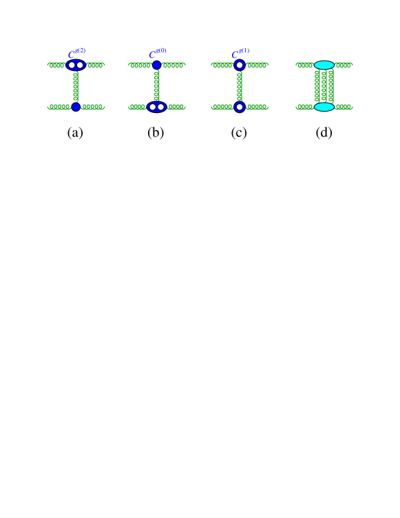
Figure 6: Additional contributions to the two-loop four-gluon amplitude at NNLL accuracy. (a, b) The two-loop impact factor is represented by the twice pierced blue blob. (c) The one-loop impact factor squared. (d) The three-Reggeized-gluon exchange.

The possibility of disentangling terms based on the exchange of one Reggeized gluon from factorization-violating terms hints that the BFKL equation, which is based on the exchange of one Reggeized gluon, may be extended to NNLL accuracy. In addition, there are reasons, based on the integrability of amplitudes in MRK in the large $N_{c}$ limit [156], to believe that Regge pole factorization will be simpler in that case. This warrants an analysis of the terms which would contribute to the BFKL equation at NNLL accuracy.

At NNLL accuracy, the kernel of the BFKL equation will have contributions from the CEV for the emission of three partons along the gluon ladder [157, 158, 159], evaluated in next-to-next-to-multi-Regge kinematics (NNMRK), fig. 7(a),

$$\ldots\gg p_{4}^{+}\simeq p_{5}^{+}\simeq p_{6}^{+}\gg\ldots\,;$$ (110)

from the one-loop corrections to the CEV for the emission of two gluons [160] or of a quark-antiquark pair along the gluon ladder, evaluated in the NMRK of eq. (71), fig. 7(b); from the two-loop corrections to the single-gluon CEV in MRK, fig. 7(c); and from the square of the one-loop five-gluon amplitude in MRK, which will contain the square of one-loop corrections to the single-gluon CEV, fig. 7(d). Once those contributions are assembled into the kernel at NNLL accuracy, the infrared divergences of the kernel must cancel the divergences of the three-loop Regge trajectory, fig. 7(e). Carrying out all the phase space integrations is a challenge for the future.

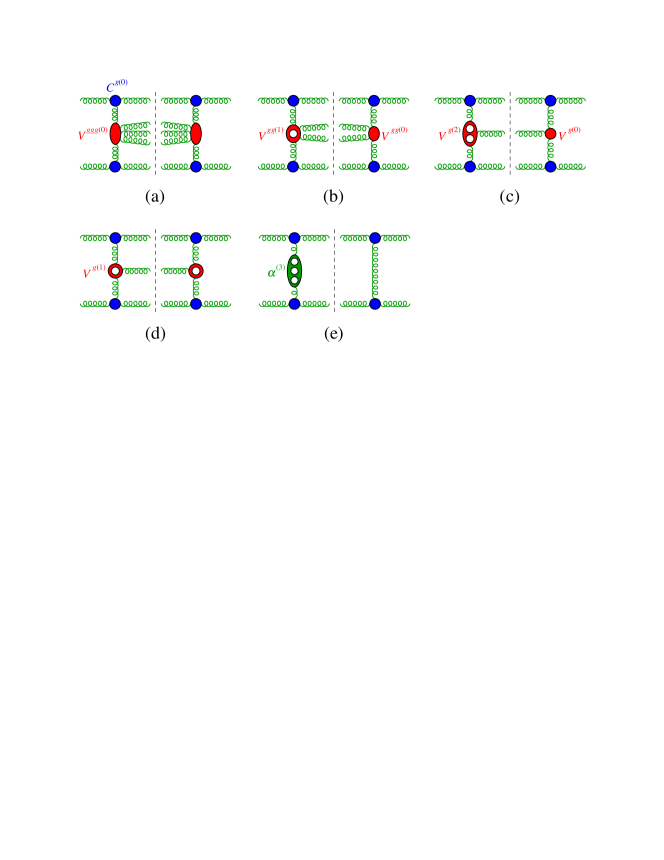
Figure 7: (a) The red blob along the gluon ladder represents the three-gluon central-emission vertex within the tree seven-gluon amplitude. (b) The pierced red blob represents the one-loop two-gluon central-emission vertex within the one-loop six–gluon amplitude. (c) The twice pierced red blob represents the two-loop central-emission vertex within the two-loop five–gluon amplitude. (d) The square of the one-loop five-gluon amplitude in MRK. (c) The thrice pierced green blob represents the three-loop gluon Regge trajectory within the three-loop four–gluon amplitude.

3 The multi-Regge limit of planar ${\cal N}=4$ SYM amplitudes

3.1 Overview

The maximally supersymmetric cousin of QCD is ${\cal N}=4$ super-Yang-Mills theory. Instead of having $n_{f}$ flavors of quarks in the fundamental representation, its matter content consists of 4 fermions (gluinos) $\Gamma_{A}$ and 6 real scalars $S_{AB}$ in the adjoint representation of the gauge group $G$. The four supersymmetries can be used to package all $2^{4}=16$ helicity states into a single on-shell superfield,

$$\Phi(k,\eta)=G^{+}+\eta^{A}\Gamma_{A}+\tfrac{1}{2!}\eta^{A}\eta^{B}S_{AB}+\tfrac{1}{3!}\eta^{A}\eta^{B}\eta^{C}\varepsilon_{ABCD}\bar{\Gamma}^{D}+\tfrac{1}{4!}\eta^{A}\eta^{B}\eta^{C}\eta^{D}\varepsilon_{ABCD}G^{-},$$ (111)

where $\eta^{A}$ is a Grassmann variable with $A=1,2,3,4$, and $\varepsilon_{ABCD}$ is the Levi-Civita antisymmetric tensor.

The large amount of supersymmetry leads to the vanishing of ultraviolet divergences, so the beta function vanishes, $\beta(g)=0$, and the theory is conformal [161, 162, 163]. If we further take the gauge group to be $G=SU(N_{c})$ and send $N_{c}\to\infty$ — the large $N_{c}$ or planar limit — then only planar Feynman diagrams contribute [164], and the ’t Hooft coupling constant is defined as

$$g^{2}\,\equiv\,\frac{\lambda}{16\pi^{2}}\,\equiv\,\frac{N_{c}g_{\scriptscriptstyle S}^{2}}{16\pi^{2}}\,=\frac{N_{c}\alpha_{\scriptscriptstyle S}}{4\pi}\,.$$ (112)

We generally take $N_{c}\to\infty$ holding $\lambda$ or $g^{2}$ fixed. In this limit, the color-decomposition of $n$-gluon amplitudes simplifies drastically, to a sum over non-cyclic permutations of single-trace terms,

$${\cal A}_{n}(a_{1},a_{2},\ldots,a_{n}) = g_{\scriptscriptstyle S}^{n-2}\sum_{\ell=0}^{\infty}g^{2\ell}\sum_{\sigma\in S_{n}/Z_{n}}{\rm Tr}(T^{a_{\sigma(1)}}T^{a_{\sigma(2)}}\cdots T^{a_{\sigma(n)}})$$ (113)

$$\hbox{}\times A_{n}^{(\ell)}(\sigma(1),\sigma(2),\ldots,\sigma(n))+{\cal O}\biggl{(}\frac{1}{N_{c}^{2}}\biggr{)}.$$

Multi-trace contributions in eq. (113) are suppressed by at least one power of $1/N_{c}^{2}$ in the color-summed cross section. Interferences between different non-cyclic orderings $\sigma$ are also color-suppressed, so the $n$ gluons can be taken to have a definite cyclic ordering, by default $1,2,\ldots,n$.

In the planar limit, ${\cal N}=4$ SYM becomes integrable [165], giving rise to additional symmetries and the prospect of solving for scattering amplitudes exactly at finite coupling. In the limit of large $\lambda$, AdS/CFT duality implies that scattering amplitudes can be computed in terms of minimal area surfaces in anti-de Sitter space, whose boundary is a closed light-like polygon [65]. This picture led to the duality between amplitudes and polygonal Wilson loops at arbitrary coupling [65, 166, 68, 167, 70, 71, 168, 169], which also implies invariance under a set of dual conformal transformations, which are distinct from, and in addition to, ordinary (position space) conformal symmetry.

These five additional dual conformal symmetries make the kinematic dependence of the four- and five-gluon amplitudes trivial. To all loop orders they are given by the Bern-Dixon-Smirnov (BDS) ansatz [72], which is essentially the exponential of the one-loop amplitude multiplied by the light-like cusp anomalous dimension $\Gamma_{\rm cusp}$, which is known to all orders in $g^{2}$ [170]. Thus the multi-loop structure of four- and five-gluon amplitudes in MRK is rather simple in planar ${\cal N}=4$ SYM: it is governed by the behavior of the one-loop amplitude and the constants in the BDS ansatz.

Starting with the six-gluon amplitude, the structure becomes much richer. In general kinematics, there are three independent dual conformally invariant cross ratios for six-gluon scattering. In an appropriate MRK limit, one of these three variables generates large logarithms in the rapidity. The coefficients of the large logarithms depend on two remaining variables parametrizing the complexified transverse momenta. The two variables lie on a complex sphere $(z,\bar{z})=(-w,-w^{\ast})$ with three punctures, at $0,1,\infty$, and the coefficients are real-analytic functions of $(z,\bar{z})$, which means that they are single-valued around all three punctures. For higher-point amplitudes, the general picture is similar. Each additional gluon adds three more variables; one is a large logarithm and two more are complex pairs. The set of punctures becomes much richer because it includes limits where different variables approach each other, as well as where they approach the three punctures.

The prospect of a finite-coupling solution for the scattering of more than five gluons has already been realized in various kinematical limits. For example, the six-gluon amplitude is dual to a hexagonal Wilson loop. The limit that two gluons become collinear is conformally equivalent to pulling apart the hexagon into two halves, separated by a long distance. In this limit, the operator product expansion (OPE) is dominated by low-twist operators [171], or flux-tube excitations, whose anomalous dimensions have been computed at finite coupling [172]. The interactions of these excitations are characterized by an integrable two-dimensional $S$ matrix, which is closely related to certain pentagon transitions. A general $n$-gluon amplitude, or Wilson $n$-gon, can be tiled by $(n-4)$ pentagons, and the resulting finite-coupling formula for the (multi) near-collinear limit is referred to as the pentagon OPE or flux-tube expansion [79, 173, 174, 175].

In the six-gluon case, the contribution of a single flux-tube excitation was analytically continued to give an all-orders proposal for the multi-Regge limit [55], which encompasses both the (adjoint) BFKL eigenvalue and the impact factor. More recently, a similar analysis was used to propose an all-orders formula for the central-emission vertex, which first enters seven-gluon MRK, and should allow an MRK description at arbitrary multiplicity and coupling. In the remainder of this section we develop these ideas further.

3.2 Six-gluon MRK

Dual conformal symmetry means that suitably normalized amplitudes have a full $SO(4,2)$ invariance that acts in momentum space, or more precisely on dual coordinates $x_{i}$, instead of the usual Poincaré invariance ($SO(3,1)$ Lorentz symmetry plus four translations). The dimension of $SO(4,2)$ is ${6\choose 2}=15$, while the Poincaré group has ${4\choose 2}+4=10$ generators. The additional five dual conformal symmetry generators consist of dilatations and four special (dual) conformal generators. The latter can be represented as an inversion $x_{i}^{\mu}\to x_{i}^{\mu}/x_{i}^{2}$, followed by an infinitesimal translation $x_{i}^{\mu}\to x_{i}^{\mu}+\epsilon^{\mu}$, followed by another inversion. Here the dual coordinates $x_{i}^{\mu}$ are the corners of the light-like polygon, so their differences are the momenta $p_{i}^{\mu}$:

$$x_{i}^{\mu}-x_{i+1}^{\mu}=p_{i}^{\mu}\,,\qquad x_{ij}^{2}=(p_{i}+p_{i+1}\cdots+p_{j-1})^{2}\,.$$ (114)

Under an inversion,

$$x_{ij}^{2}\to\frac{x_{ij}^{2}}{x_{i}^{2}x_{j}^{2}}\,.$$ (115)

Dual conformally invariant functions are functions $f(u_{ijkl})$ of the cross ratios

$$u_{ijkl}\equiv\frac{x_{ij}^{2}x_{kl}^{2}}{x_{ik}^{2}x_{jl}^{2}}\,,$$ (116)

because under the inversion (115) the factors of $x_{i}^{2}x_{j}^{2}x_{k}^{2}x_{l}^{2}$ cancel between numerator and denominator.

In four dimensions, the number of kinematic variables for a Poincaré-invariant $n$-point process is $3n-10$: $3n$ for the spatial momentum components of the $n$-particles (which determine the energies), minus 10 for the symmetries. This formula gives 2 for the 4-point process, namely the familiar Mandelstam variables $s$ and $t$ (with $u=-s-t$ in the massless case), and 5 for the 5-point process, which could be taken to be $s_{i,i+1}=(p_{i}+p_{i+1})^{2}$, $i=1,2,\ldots,5$. The five additional symmetry generators of dual conformal invariance reduce the number of kinematic variables by five more, to $3n-15$. There are no variables left for $n=4$ or 5, and the (MHV) amplitudes are given by the BDS ansatz [72],

$$A_{n}^{\rm BDS}=A_{n}^{(0)}\,\text{exp}\left[\sum_{\ell=1}^{\infty}g^{2\ell}\left(f^{(\ell)}(\epsilon)M_{n}^{(1)}(\ell\epsilon)+C^{(\ell)}\right)\right]\,,$$ (117)

where $A_{n}^{(0)}$ is the tree-level Parke-Taylor amplitude [176], $M_{n}^{(1)}(\epsilon)$ is the one-loop MHV amplitude (divided by the tree) [177],

$$f^{(\ell)}(\epsilon)=f_{0}^{(\ell)}+\epsilon\,f_{1}^{(\ell)}+\epsilon^{2}\,f_{2}^{(\ell)}$$ (118)

is a set of three constants, and $C^{(\ell)}$ is an additional, finite constant. Here $f_{0}$ is the cusp anomalous dimension, known to all orders in perturbation theory [170],

$$f_{0}(g^{2})\,\equiv\,\Gamma(g^{2})\,=\,\frac{\Gamma_{\rm cusp}(g^{2})}{4}\,=\,g^{2}-2\,\zeta_{2}\,g^{4}+22\,\zeta_{4}\,g^{6}-(219\,\zeta_{6}+8\,\zeta_{3}^{2})\,g^{8}+\cdots\,.$$ (119)

The convention for normalizing the cusp anomalous dimension in planar ${\cal N}=4$ differs from that in QCD by a factor of two:

$$\gamma_{K}\ =\ 2\,\Gamma_{\rm cusp}\,.$$ (120)

In eq. (118), $f_{1}^{(\ell)}$ is related to the gluon collinear anomalous dimension defined in eq. (61) by

$$f_{1}^{(\ell)}\ =\ -\frac{\ell}{2}\,\gamma_{g}^{(\ell)\,{\cal N}=4}\ =\ \frac{\ell}{4}{\cal G}_{0}^{(\ell)\,{\cal N}=4}\,,$$ (121)

where the second definition is used in e.g. ref. [178]. It is known to four loops [179, 178, 180]. The finite constants $f_{2}^{(\ell)}$ and $C^{(\ell)}$ are known (numerically) to three loops [72, 181].

The BDS ansatz provides the complete amplitude for $n=4$ and 5 because it is the unique solution to an anomalous dual conformal Ward identity [68]. Starting at $n=6$, the solution is not unique, because of the existence of three dual conformal cross ratios,

$$u_{1}=\frac{x_{13}^{2}x_{46}^{2}}{x_{14}^{2}x_{36}^{2}}=\frac{s_{12}s_{45}}{s_{123}s_{345}}\,,\qquad u_{2}=\frac{x_{24}^{2}x_{51}^{2}}{x_{25}^{2}x_{41}^{2}}=\frac{s_{23}s_{56}}{s_{234}s_{123}}\,,\qquad u_{3}=\frac{x_{35}^{2}x_{62}^{2}}{x_{36}^{2}x_{52}^{2}}=\frac{s_{34}s_{61}}{s_{345}s_{234}}\,.$$ (122)

The full six-point amplitude can be written as

$$A_{6}^{\rm MHV}(s_{i,j},\epsilon)=A_{6}^{\rm BDS}(s_{i,j},\epsilon)\,\exp\Bigl{[}R_{6}(u_{1},u_{2},u_{3})\Bigr{]}\,,$$ (123)

where $R_{6}$ is the remainder function. The six-point one-loop amplitude entering the BDS ansatz is

$$M_{6}^{(1)} = \hat{M}_{6}^{(1)}\,+\,{\cal E}_{6}^{(1)}(u_{i})\,,$$ (124)

$$\hat{M}_{6}^{(1)} = \sum_{i=1}^{6}\biggl{[}-\frac{1}{\epsilon^{2}}+\frac{\ln(-s_{i,i+1})}{\epsilon}-\ln(-s_{i,i+1})\Bigl{(}\ln(-s_{i+1,i+2})-\frac{1}{2}\ln(-s_{i+3,i+4})\Bigr{)}\biggr{]}+6\zeta_{2}\,,$$

where

$${\cal E}_{6}^{(1)}=\sum_{i=1}^{3}{\rm Li}_{2}\biggl{(}1-\frac{1}{u_{i}}\biggr{)}\,.$$ (125)

It is also possible to normalize by a BDS-like ansatz [108, 84], which uses $\hat{M}_{6}^{(1)}$ instead of $M_{6}^{(1)}$ in eq. (117), thus omitting the finite, dual conformally invariant part ${\cal E}_{6}^{(1)}$ of the one-loop amplitude. This normalization leads to improved causal properties for bootstrapping at generic kinematics; namely, the Steinmann relations remain manifest [51]. However, for discussing MRK the remainder function $R_{6}$ is more suitable, because it vanishes in all collinear and soft limits, and a soft limit is equivalent to a Euclidean version of MRK.

There are various possible six-point MRK limits, but the one that gives rise to the most interesting behavior [73] is the case of $2\to 4$ scattering when the two incoming gluons are as far as they can get from each other in the cyclic color ordering. For the cyclic color ordering $1,2,\ldots,6$, we take gluons 3 and 6 to be incoming and gluons $1,2,4,5$ outgoing. (This configuration is sometimes also described by starting with the process $1+2\to 3+4+5+6$, and moving legs 4 and 5 into the initial state, between legs 1 and 2.) The strong rapidity ordering for MRK, in terms of color-ordered Mandelstam variables, is

$$s_{12}\gg s_{345},s_{123}\gg s_{34},s_{45},s_{56}\gg s_{23},s_{61},s_{234}\,.$$ (126)

In terms of the cross ratios (122), the limit is

$$u_{1}\to 1,\qquad u_{2}\to 0,\qquad u_{3}\to 0,$$ (127)

with $u_{2}/(1-u_{1})$ and $u_{3}/(1-u_{1})$ held fixed. It is important to note that while $s_{12}$ and $s_{45}$ are positive, the rest of the invariants listed in eq. (126) are negative. These sign assignments in eq. (122) lead to $u_{1},u_{2},u_{3}>0$.

There is an unphysical Euclidean branch, or Riemann sheet, where all Mandelstam invariants are spacelike, and so $u_{1},u_{2},u_{3}>0$ there as well. On the Euclidean sheet, all loop integrals are real, and hence the scattering amplitude is real. The $2\to 4$ sheet for physical Minkowski scattering is on a different Riemann sheet from the Euclidean sheet, despite also having $u_{1},u_{2},u_{3}>0$. (Physical $2\to 4$ scattering also requires $u_{1},u_{2},u_{3}<1$ and $\Delta<0$, where $\Delta$ is given in eq. (131) [160].) Because $u_{1}$ in eq. (122) contains two positive (timelike) invariants in the numerator, and two negative (spacelike, or Euclidean) invariants in the denominator, it has to be continued by wrapping once around the complex origin,

$$u_{1}\to u_{1}e^{-2\pi i}\,.$$ (128)

On the other hand, $u_{2}$ and $u_{3}$ are composed entirely of spacelike invariants, so they do not have to be continued at all from the Euclidean sheet. The analytic continuation (128) generates discontinuities that diverge in MRK, even though the remainder function $R_{6}$ vanishes in the same limit (127) on the Euclidean sheet.

The finite, dual conformally invariant part of six-gluon scattering amplitudes in planar ${\cal N}=4$ SYM in the “bulk”, i.e. for arbitrary kinematics, are built from a polylogarithmic function space described by nine letters:

$${\cal S}_{\rm hex}=\{u_{i}\,,1-u_{i}\,,y_{i}\},\quad i=1,2,3,$$ (129)

where

$$y_{i} = \frac{u_{i}-z_{+}}{u_{i}-z_{-}}\,,\qquad z_{\pm}=\frac{-1+u_{1}+u_{2}+u_{3}\pm\sqrt{\Delta}}{2}\,,$$ (130)

$$\Delta = (1-u_{1}-u_{2}-u_{3})^{2}-4u_{1}u_{2}u_{3}\,.$$ (131)

As reviewed in Chapter 5 of this SAGEX Review [86], the meaning of the symbol alphabet ${\cal S}$ [80] is that every function $F$ in the corresponding function space has a “d log” derivative structure with a finite number of terms,

$$dF=\sum_{s_{k}\in{\cal S}}F^{s_{k}}\ d\ln s_{k}\,,$$ (132)

where $s_{k}$ are the symbol letters, and if $F$ has weight $n$ then $F^{s_{k}}$ has weight $n-1$.

The $y_{i}$ letters are fairly complicated in the bulk, at least in terms of the cross-ratios $u_{i}$. (All 9 letters can be parametrized rationally in the bulk using the $y_{i}$ variables [47], or momentum twistors, which are associated with the Grassmannian ${\rm Gr}(4,6)$, see e.g. ref. [183], or the pentagon OPE parametrization in refs. [79, 173].)

Here we only need to parametrize the MRK limit (127). It is convenient to take

$$\frac{u_{2}}{1-u_{1}}=\frac{1}{(1-z)(1-\bar{z})}\,,\qquad\frac{u_{3}}{1-u_{1}}=\frac{z\bar{z}}{(1-z)(1-\bar{z})}\,,$$ (133)

as this rationalizes $\sqrt{\Delta}\approx(1-u_{1})(z-\bar{z})/|1-z|^{2}$. Thus the $y_{i}$ become rational too,

$$y_{1}\to 1\,,\qquad y_{2}\to\frac{1-\bar{z}}{1-z}\,,\qquad y_{3}\to\frac{(1-z)\bar{z}}{(1-\bar{z})z}\,,$$ (134)

and they are pure phases when $\bar{z}$ is the complex conjugate of $z$.

It is apparent from eqs. (133) and (134) that the bulk symbol alphabet (129) collapses in MRK to the four letters

$${\cal S}_{\rm hex,\,MRK}=\{z,1-z,\bar{z},1-\bar{z}\}\,.$$ (135)

There is also the infinitesimal letter $(1-u_{1})$, but it just corresponds to free powers of $\ln(1-u_{1})$. Using the characterization (132), the derivatives of any function in this space have the form

$$\frac{\partial F}{\partial z}=\frac{F^{z}}{z}-\frac{F^{1-z}}{1-z}\,,\qquad\frac{\partial F}{\partial\bar{z}}=\frac{F^{\bar{z}}}{\bar{z}}-\frac{F^{1-\bar{z}}}{1-\bar{z}}\,.$$ (136)

These relations imply that the relevant function space must be built from HPLs [148] in $z$ and $\bar{z}$.

HPLs with indices $\{0,1\}$ are defined for binary strings $\vec{w}$ with elements $w_{k}\in\{0,1\}$. They are defined iteratively by

$$H_{0,\vec{w}}(z)=\int_{0}^{z}\frac{dt}{t}H_{\vec{w}}(t),\qquad H_{1,\vec{w}}(z)=\int_{0}^{z}\frac{dt}{1-t}H_{\vec{w}}(t),$$ (137)

as well as the initial condition $H(z)=1$ for the null string, and the special case of all zeroes,

$$H_{\vec{0}_{n}}(z)=\frac{1}{n!}\ln^{n}z\,.$$ (138)

The weight of $H_{\vec{w}}$ is the number of integrations, or the length $|\vec{w}|$ of the binary string $\vec{w}$. HPLs obey the differential relations,

$$\frac{\partial H_{0,\vec{w}}(z)}{\partial z}=\frac{H_{\vec{w}}(z)}{z}\,,\qquad\frac{\partial H_{1,\vec{w}}(z)}{\partial z}=\frac{H_{\vec{w}}(z)}{1-z}\,,$$ (139)

which matches the structure of eq. (136). Thus the relevant MRK function space involves a tensor product of the singular logarithm, HPLs in $z$, and HPLs in $\bar{z}$:

$${\cal F}_{\rm MRK}\subset\left\{\ln^{k}(1-u_{1}),\ k\geq 0\right\}\otimes\left\{H_{\vec{w}}(z),\ w_{k}\in\{0,1\}\right\}\otimes\left\{H_{\vec{w}}(\bar{z}),\ w_{k}\in\{0,1\}\right\}\,.$$ (140)

At weight $n$, there are $2^{n}$ possible HPLs with indices $\{0,1\}$. They obey a shuffle algebra, so that

$$H_{\vec{w}_{1}}(z)\,H_{\vec{w}_{2}}(z)=\sum_{w\in w_{1}\mbox{\bf\scyr X}w_{2}}H_{\vec{w}}(z)\,,$$ (141)

where ${w_{1}}{\mbox{\cyr X}}{w_{2}}$ is the set of shuffles, or mergers of the sequences $w_{1}$ and $w_{2}$ that preserve their individual orderings. Equation (141) can be used, from right to left, to express the $2^{n}$ functions in terms of sums and products of a much smaller set of functions, which is called the Lyndon basis, because there is one $H_{\vec{w}_{L}}$ for each Lyndon word. Lyndon words $w_{L}$, when split into any two sub-words $u$ and $v$, always have $u<v$ lexicographically. The number of binary Lyndon words for weight $1,2,3,\ldots$ is $2,1,2,3,6,9,18,30,\ldots$. The first few Lyndon words are $w_{L}=0,1;01;001,011;0001,0011,0111$. The linear basis is obtained by applying eq. (141) repeatedly from left to right, so that there are no more products.

Eq. (140) is not the whole story; there is one more restriction, single-valuedness, which is related to the location of branch cuts. On the Euclidean sheet, for massless scattering amplitudes, branch cuts originate when Mandelstam variables vanish, since that is where physical scattering can first turn on. Given eq. (122), these cuts can only originate at $u_{i}=0$ or $u_{i}=\infty$. In the symbol, branch cut locations correspond to the vanishing of first entries (or their inverses), leading to the first-entry condition [184] which for general six-point kinematics states that only the symbol letters $u_{i}$ in eq. (129) are allowed to occupy the first entry in any term in the symbol, not $1-u_{i}$ nor $y_{i}$. In fact, the $y_{i}$ letters do not actually appear until the third entry, because of integrability (equality of mixed partial derivatives). When the analytic continuation (128) is performed, at symbol level it corresponds to clipping off a $u_{1}$ from the front of the symbol, exposing the second entry. Because this entry is always a $u_{i}$ or $1-u_{i}$, as one takes the limit (133), the first entry always involves the pairs $z\bar{z}$ and $(1-z)(1-\bar{z})$. Functions whose symbol letters are given by ${\cal S}_{\rm hex,\,MRK}$ in eq. (135), but with first entries restricted to $z\bar{z}$ and $(1-z)(1-\bar{z})$, are called single-valued HPLs (SVHPLs) [88, 54] and denoted by ${\cal L}_{\vec{w}}(z,\bar{z})$. They do not have branch cuts separately in $z$ and $\bar{z}$; for example, when $z$ is continued around the origin, and $\bar{z}$ is continued in the opposite direction, the functions remain single-valued, so they are real analytic on the punctured complex plane, $\mathbb{C}/\{0,1,\infty\}$.

The functions ${\cal L}_{\vec{w}}(z,\bar{z})$ obey same differential relations in $z$ as $H_{\vec{w}}(z)$:

$$\frac{\partial{\cal L}_{0,\vec{w}}(z)}{\partial z}=\frac{{\cal L}_{\vec{w}}(z)}{z}\,,\qquad\frac{\partial{\cal L}_{1,\vec{w}}(z)}{\partial z}=\frac{{\cal L}_{\vec{w}}(z)}{1-z}\,.$$ (142)

They also obey the “initial conditions”

$${\cal L}(z)=1,\qquad{\cal L}_{\vec{0}_{n}}(z)=\frac{1}{n!}\ln^{n}|z|^{2}\,,\qquad\lim_{z\rightarrow 0}{\cal L}_{\vec{w}\neq\vec{0}_{n}}(z)=0,$$ (143)

and the same shuffle relations as the HPLs,

$${\cal L}_{\vec{w}_{1}}(z)\,{\cal L}_{\vec{w}_{2}}(z)=\sum_{w\in w_{1}\mbox{\bf\scyr X}w_{2}}{\cal L}_{\vec{w}}(z)\,,$$ (144)

These conditions, real analyticity on $\mathbb{C}/\{0,1,\infty\}$, and the differential relation (142), fix the ${\cal L}_{\vec{w}}(z,\bar{z})$.

Each ${\cal L}_{\vec{w}}$ is a weight $|\vec{w}|$ linear combination of products of HPLs in $z$, HPLs in $\bar{z}$, and multiple zeta values. The fully holomorphic part of ${\cal L}_{\vec{w}}(z,\bar{z})$ is precisely $H_{\vec{w}}(z)$. The full construction of ${\cal L}_{\vec{w}}$ [88] relies on the single-valued map ${\bf s}$ mentioned in sec. 2.7. It incorporates the antipode map (which reverses the order of letters in the symbol) and the Drin’feld associator, which is a formal sum of values of the HPLs at unit argument, $H_{\vec{w}}(1)=\zeta(\vec{w})$.

It is useful to introduce a collapsed notation which maps a string of $(m-1)$ 0’s followed by a 1 to the integer $m$:

$$\ldots,\vec{0}_{m-1},1,\ldots\ \to\ \ldots,m,\ldots$$ (145)

In this notation, $\zeta(\vec{w})$ can be identified with the multiple zeta values (MZVs) defined by the nested sums,

$$\zeta_{m_{1},\ldots,m_{k}}=\zeta(m_{1},\ldots,m_{k})=\sum_{\infty>i_{1}>i_{2}>\cdots>i_{k}>0}\frac{1}{i_{1}^{m_{1}}i_{2}^{m_{2}}\cdots i_{k}^{m_{k}}}\,.$$ (146)

Next we give a few explicit examples of ${\cal L}_{\vec{w}}\equiv{\cal L}_{\vec{w}}(z,\bar{z})$ [88], defining $H_{\vec{w}}\equiv H_{\vec{w}}(z)$ and ${\overline{H}}_{\vec{w}}=H_{\vec{w}}(\bar{z})$. At weight one, there is only

$${\cal L}_{0}\;=\;H_{0}+{\overline{H}}_{0}\;=\;\ln|z|^{2}\,,\qquad{\cal L}_{1}\;=\;H_{1}+{\overline{H}}_{1}\;=\;-\ln|1-z|^{2}\,.$$ (147)

The SVHPLs of weight two begin to expose the order-reversal in the antipode map,

$${\cal L}_{0,0} = H_{0,0}+{\overline{H}}_{0,0}+H_{0}{\overline{H}}_{0}\,,\qquad{\cal L}_{0,1}\;=\;H_{0,1}+{\overline{H}}_{1,0}+H_{0}{\overline{H}}_{1}\,,$$

$${\cal L}_{1,0} = H_{1,0}+{\overline{H}}_{0,1}+H_{1}{\overline{H}}_{0}\,,\qquad{\cal L}_{1,1}\;=\;H_{1,1}+{\overline{H}}_{1,1}+H_{1}{\overline{H}}_{1}\,.$$ (148)

Thanks to the shuffle relations (141) and (144), it is enough to give results for the Lyndon basis only, which at weight three is,

$${\cal L}_{0,0,1} \;=\;H_{0,0,1}+{\overline{H}}_{1,0,0}+H_{0,0}{\overline{H}}_{1}+H_{0}{\overline{H}}_{1,0}\,,$$

$${\cal L}_{0,1,1} \;=\;H_{0,1,1}+{\overline{H}}_{1,1,0}+H_{0,1}{\overline{H}}_{1}+H_{0}{\overline{H}}_{1,1}\,,$$ (149)

and at weight four it is,

$${\cal L}_{0,0,0,1} = H_{0,0,0,1}+{\overline{H}}_{1,0,0,0}+H_{0,0,0}{\overline{H}}_{1}+H_{0}{\overline{H}}_{1,0,0}+H_{0,0}{\overline{H}}_{1,0}\,,$$

$${\cal L}_{0,0,1,1} = H_{0,0,1,1}+{\overline{H}}_{1,1,0,0}+H_{0,0,1}{\overline{H}}_{1}+H_{0}{\overline{H}}_{1,1,0}+H_{0,0}{\overline{H}}_{1,1}-2\zeta_{3}\,{\overline{H}}_{1}\,,$$

$${\cal L}_{0,1,1,1} = H_{0,1,1,1}+{\overline{H}}_{1,1,1,0}+H_{0,1,1}{\overline{H}}_{1}+H_{0}{\overline{H}}_{1,1,1}+H_{0,1}{\overline{H}}_{1,1}-2\zeta_{3}\,{\overline{H}}_{1}\,,$$ (150)

at which point explicit $\zeta$ values from the Drin’feld associator start to appear.

In summary, the function space for six-point amplitudes in planar ${\cal N}=4$ SYM in MRK reduces from (140) to

$${\cal F}_{\rm MRK}\subset\left\{\ln^{k}(1-u_{1}),\ k\geq 0\right\}\otimes\left\{{\cal L}_{\vec{w}}(z),\ w_{k}\in\{0,1\}\right\}\,,$$ (151)

including also the possibility of MZV constants. Note that we can easily trade $(1-u_{1})$ for $\sqrt{u_{2}u_{3}}$ because the ratio is finite, from eq. (133), and its logarithm is in the space of SVHPLs,

$$\ln(\sqrt{u_{2}u_{3}})-\ln(1-u_{1})=\frac{1}{2}\ln|z|^{2}-\ln|1-z|^{2}=\frac{1}{2}{\cal L}_{0}+{\cal L}_{1}\,.$$ (152)

It is convenient to define a large logarithm by

$$L_{\tau}\,\equiv\,\ln\tau,\qquad\tau\equiv\sqrt{u_{2}u_{3}}\,.$$ (153)

The six-gluon remainder function $R_{6}(u,v,w)$ vanishes in the Euclidean version of the MRK limit, which is a soft limit, a special case of the collinear limit, where it also vanishes. It also vanishes exactly at one loop, by definition. It is also possible to argue from the OPE perspective that the leading power of the singular logarithm at $\ell$ loops should be $\ell-1$ [171]. From these properties, and the general structure of the function space (151), we can write the general form of the remainder function in MRK as

$$R_{6}|_{\rm MRK}=2\pi i\sum_{\ell=2}^{\infty}\sum_{n=0}^{\ell-1}g^{2\ell}\ln^{n}(1-u_{1})\Bigl{[}g_{n}^{(\ell)}(z,\bar{z})+2\pi ih_{n}^{(\ell)}(z,\bar{z})\Bigr{]}\,,$$ (154)

where the imaginary part $g_{n}^{(\ell)}$ (real part $h_{n}^{(\ell)}$) is a weight $2\ell-n-1$ ($2\ell-n-2$) linear combination of SVHPLs. The overall $2\pi i$ comes from having to take at least a single discontinuity under the continuation (128); the second discontinuity contributes to $h_{n}^{(\ell)}$; and higher odd (even) discontinuities also contribute to $g_{n}^{(\ell)}$ ($h_{n}^{(\ell)}$). The leading logarithmic (LL) coefficients clearly have $n=\ell-1$; the next-to-leading logarithmic (NLL) coefficients have $n=\ell-2$; and the N^kLL coefficients have $n=\ell-k-1$. Hence the N^kLL coefficient $g_{\ell-k-1}^{(\ell)}$ has weight $\ell+k$.

An all-loop integral formula for the six-point amplitude in MRK, based on factorization in Fourier-Mellin space, was first presented at NLL in refs. [75, 76], and argued to hold for all subleading logarithms in ref. [185]. It takes the form (after letting $w=-z$, $w^{\ast}=-\bar{z}$) [96],

$$e^{R_{6}+i\delta_{6}}|_{\textrm{MRK}} = \cos\Bigl{(}\pi\Gamma\ln|z|^{2}\Bigr{)}$$

$$\hskip 0.0pt+i\,g^{2}\sum_{m=-\infty}^{\infty}\left(\frac{z}{\bar{z}}\right)^{{m\over 2}}{\cal P}\int_{-\infty}^{\infty}\frac{d\nu\,|z|^{2i\nu}}{\nu^{2}+\frac{m^{2}}{4}}\Phi_{\textrm{reg}}(\nu,m)e^{-(L_{\tau}+i\pi)\omega(\nu,m)}\,,$$

where ${\cal P}$ is a principal value prescription for the $m=0$ term, and $L_{\tau}$ is defined in eq. (153). The first and second terms are called, respectively, the Regge pole and cut contributions. The latter depends on the BFKL eigenvalue $\omega(\nu,m)$ and the (regularized) impact factor $\Phi_{\textrm{reg}}(\nu,m)$; the latter is really a product of impact factors for the top and bottom of the Regge ladder shown in fig. 8. Both $\omega$ and $\Phi_{\textrm{reg}}$ depend on $g^{2}$. The function $\delta_{6}$ appearing on the left-hand side of eq. (3.2) comes from a Mandelstam cut present in the BDS ansatz; it is given by

$$\delta_{6}=\pi\Gamma(g^{2})\,\ln\biggl{(}\frac{|z|^{2}}{|1-z|^{4}}\biggr{)}\,,$$ (156)

where $\Gamma(g^{2})$ is defined in eq. (119).

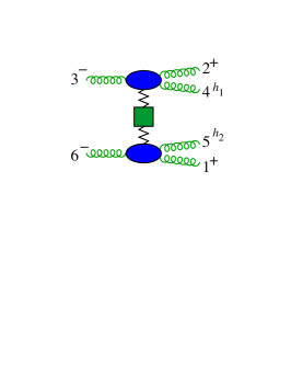
Figure 8: Factorization of the six-gluon amplitude in planar ${\cal N}=4$ SYM in the $2\to 4$ multi-Regge limit. The product of the upper and lower impact factors (blue blobs) is given by $\Phi_{\textrm{reg}}$ in the MHV case $(h_{1},h_{2})=({+},{+})$, while the zigzag line and the green square represent the Reggeized gluon in the adjoint representation and its BFKL eigenvalue. In contrast to the previous figures, a blob represents all loop orders at once. Also, there are vertical cuts through the Reggeized gluon that are not shown.

In the all-orders solution from the flux-tube representation [55], the Mellin variable $\nu$ and BFKL eigenvalue $\omega$ are related to the energy and momenta of an analytically-continued flux-tube excitation, characterized by a rapidity $u$. They are both given in terms of the kernel $K(t)$ entering the BES integral equation [170],

$$-\omega(u,m) = \int_{0}^{\infty}\frac{dt}{t}\biggl{(}\frac{K(-t)+K(t)}{2}\cos(ut)e^{-|m|t/2}-K(t)\biggr{)}\,,$$ (157)

$$\nu(u,m) = u+\int_{0}^{\infty}\frac{dt}{t}\frac{K(-t)-K(t)}{4}\sin(ut)e^{-|m|t/2}\,.$$ (158)

The impact factor is given in terms of the “measure” $\mu^{\rm BFKL}$, which involves a few more ingredients [55]. The full formula for $R_{6}$ in MRK is

$$e^{R_{6}+i\delta_{6}}|_{\textrm{MRK}}=i\,\sum_{m=-\infty}^{\infty}\left(\frac{z}{\bar{z}}\right)^{{m\over 2}}\int_{-\infty}^{\infty}du\,\mu^{\rm BFKL}(u,m)\,|z|^{2i\nu(u,m)}\,e^{-(L_{\tau}+i\pi)\omega(u,m)}\,.$$ (159)

The Regge pole contribution in eq. (3.2) is not present explicitly in eq. (159), but it is generated by a different contour prescription for the $u$ integral [55, 96].

The BES kernel $K(t)$ can be represented as a semi-infinite matrix of integrals of products of Bessel functions [186]. At weak coupling, the matrix can be truncated to a finite size, allowing perturbative expansions of $\nu(u,m)$, $\omega(u,m)$ and $\mu^{\rm BFKL}(u,m)$ to any desired order in the loop expansion [55]. The results are polynomials in $E,V,N$ [54] defined by

$$E = -\frac{1}{2}\frac{|m|}{u^{2}+\frac{m^{2}}{4}}+\psi(1+iu+\tfrac{|m|}{2})+\psi(1-iu+\tfrac{|m|}{2})-2\psi(1),$$ (160)

$$V = \frac{iu}{u^{2}+\frac{m^{2}}{4}}\,,\qquad N=\frac{m}{u^{2}+\frac{m^{2}}{4}}\,,$$ (161)

and their $u$ derivatives, with $D\equiv-i\partial/\partial u$. The results for $\nu$ and $\omega$ through $g^{6}$ are [55],

$$2\nu = 2u+2ig^{2}V-ig^{4}(D^{2}V+4\zeta_{2}V)$$ (162)

$$\hskip 0.0pt\hbox{}+ig^{6}\biggl{(}\frac{1}{6}D^{4}V+2\zeta_{2}D^{2}V-4\zeta_{3}DE+44\zeta_{4}V\biggr{)}+\ldots,$$

$$-\omega = 2g^{2}E-g^{4}(D^{2}E+4\zeta_{2}E+12\zeta_{3})$$ (163)

$$\hskip 0.0pt\hbox{}+g^{6}\biggl{(}\frac{1}{6}D^{4}E+2\zeta_{2}D^{2}E+4\zeta_{3}DV+44\zeta_{4}E+80\zeta_{5}+16\zeta_{2}\zeta_{3}\biggr{)}+\ldots.$$

Using eq. (162), one can eliminate $u$ in favor of $\nu$ order by order in the coupling, in order to obtain the more standard definition of the BFKL eigenvalue $\omega(\nu,m)$ as functions of $E,V,N$ that depend on $\nu$ instead of $u$. The results agree with previous computations through NNLL [73, 74, 76, 54, 83]. The relation between the BFKL measure and the impact factor is

$$\mu^{\rm BFKL}(u,m)\,=\,g^{2}\frac{d\nu}{du}\frac{\Phi_{\textrm{reg}}(\nu,m)}{\nu^{2}+\frac{m^{2}}{4}}\,.$$ (164)

This impact factor agrees with previous computations at low loop orders [75, 54, 83].

Once the perturbative expansions of $\omega(\nu,m)$ and $\Phi_{\textrm{reg}}(\nu,m)$ have been obtained, the inverse FM sum-integral in eq. (3.2) has to be performed. It can be converted into a double sum by closing the $\nu$ contour with a large semi-circle in the complex plane and picking up residues from integer-spaced poles on the positive imaginary axis. Truncating the sum over residues corresponds to performing a series expansion as $z,\bar{z}\to 0$. Methods for performing this sum have been given in refs. [54, 90, 91, 56]. Alternatively, if one has the perturbative amplitude, the coefficient functions can be computed, without having to perform any sums, by taking the multi-Regge limit of the result for general kinematics. It is straightforward to series expand the coefficient functions as $z,\bar{z}\to 0$, to compare with the FM representation. The results match through seven loops [52].

Defining the FM sum $\Sigma$ via,

$$e^{R_{6}+i\delta_{6}}|_{\textrm{MRK}}\ = \ \cos\Bigl{(}\pi\Gamma\ln|z|^{2}\Bigr{)}+\pi i\,\Sigma\,,$$

$$\hskip 28.45274pt\Sigma\ = \ \sum_{\ell=1}^{\infty}g^{2\ell}\sum_{n=0}^{\ell-1}\Sigma_{n}^{(\ell)}\,(L_{\tau}+i\pi)^{n}\,,$$ (165)

the first three loop orders are given in the linear SVHPL representation by,

$$\Sigma_{0}^{(1)} = {\cal L}_{0}+2{\cal L}_{1}\,,$$ (166)

$$\Sigma_{1}^{(2)} = 2{\cal L}_{0,1}+2{\cal L}_{1,0}+4{\cal L}_{1,1}\,,$$ (167)

$$\Sigma_{0}^{(2)} = -2{\cal L}_{0,0,1}+2{\cal L}_{0,1,0}-2{\cal L}_{0,1,1}-2{\cal L}_{1,0,0}-2{\cal L}_{1,0,1}-2{\cal L}_{1,1,0}-4{\cal L}_{1,1,1}$$ (168)

$$\hskip 0.0pt\hbox{}-2\zeta_{2}({\cal L}_{0}+2{\cal L}_{1})\,,$$

$$\Sigma_{2}^{(3)} = {\cal L}_{0,0,1}+2{\cal L}_{0,1,0}+4{\cal L}_{0,1,1}+{\cal L}_{1,0,0}+4{\cal L}_{1,0,1}+4{\cal L}_{1,1,0}+8{\cal L}_{1,1,1}\,,$$ (169)

$$\Sigma_{1}^{(3)} = -3{\cal L}_{0,0,0,1}+{\cal L}_{0,0,1,0}-6{\cal L}_{0,0,1,1}+{\cal L}_{0,1,0,0}-4{\cal L}_{0,1,0,1}-12{\cal L}_{0,1,1,1}$$ (170)

$$\hskip 0.0pt\hbox{}-3{\cal L}_{1,0,0,0}-8{\cal L}_{1,0,0,1}-4{\cal L}_{1,0,1,0}-12{\cal L}_{1,0,1,1}-6{\cal L}_{1,1,0,0}-12{\cal L}_{1,1,0,1}$$

$$\hskip 0.0pt\hbox{}-12{\cal L}_{1,1,1,0}-24{\cal L}_{1,1,1,1}+4\zeta_{3}{\cal L}_{1}-8\zeta_{2}({\cal L}_{0,1}+{\cal L}_{1,0}+2{\cal L}_{1,1})\,,$$

$$\Sigma_{0}^{(3)} = 3{\cal L}_{0,0,0,0,1}-\frac{9}{2}{\cal L}_{0,0,0,1,0}+3{\cal L}_{0,0,0,1,1}+5{\cal L}_{0,0,1,0,0}+3{\cal L}_{0,0,1,0,1}$$ (171)

$$\hskip 0.0pt\hbox{}-{\cal L}_{0,0,1,1,0}+6{\cal L}_{0,0,1,1,1}+2{\cal L}_{0,1,0,0,1}-\frac{9}{2}{\cal L}_{0,1,0,0,0}-2{\cal L}_{0,1,0,1,0}$$

$$\hskip 0.0pt\hbox{}+4{\cal L}_{0,1,0,1,1}-{\cal L}_{0,1,1,0,0}+4{\cal L}_{0,1,1,0,1}+12{\cal L}_{0,1,1,1,1}+3{\cal L}_{1,0,0,0,0}$$

$$\hskip 0.0pt\hbox{}+6{\cal L}_{1,0,0,0,1}+2{\cal L}_{1,0,0,1,0}+8{\cal L}_{1,0,0,1,1}+3{\cal L}_{1,0,1,0,0}+8{\cal L}_{1,0,1,0,1}$$

$$\hskip 0.0pt\hbox{}+4{\cal L}_{1,0,1,1,0}+12{\cal L}_{1,0,1,1,1}+3{\cal L}_{1,1,0,0,0}+8{\cal L}_{1,1,0,0,1}+4{\cal L}_{1,1,0,1,0}$$

$$\hskip 0.0pt\hbox{}+12{\cal L}_{1,1,0,1,1}+6{\cal L}_{1,1,1,0,0}+12{\cal L}_{1,1,1,0,1}+12{\cal L}_{1,1,1,1,0}+24{\cal L}_{1,1,1,1,1}$$

$$\hskip 0.0pt\hbox{}-2\zeta_{2}(3{\cal L}_{0,0,0}+2{\cal L}_{0,1,0}-4{\cal L}_{0,1,1}-4{\cal L}_{1,0,1}-4{\cal L}_{1,1,0}-8{\cal L}_{1,1,1})$$

$$\hskip 0.0pt\hbox{}+2\zeta_{3}({\cal L}_{0,1}+{\cal L}_{1,0}-2{\cal L}_{1,1})+22\zeta_{4}({\cal L}_{0}+2{\cal L}_{1})\,.$$

Results through seven loops are provided in an ancillary file for ref. [52], although for a slightly different normalization, coupling-constant convention, and ${\cal L}$ representation. At LL, only the Regge cut contributes and $e^{R_{6}}\approx 1+R_{6}$; hence the coefficients $\Sigma_{\ell-1}^{(\ell)}$ are simply related to the corresponding coefficients in the expansion of the remainder function $R_{6}$ in eq. (154):

$$\Sigma_{\ell-1}^{(\ell)}=2g_{\ell-1}^{(\ell)}\,.$$ (172)

These LL coefficients are known in closed form to all loop orders [133, 91].

The MRK limit of $3\to 3$ scattering is closely related. There are some sign flips associated with an analytic continuation of $u_{1}$ in the opposite direction, $u_{1}\to u_{1}e^{+2\pi i}$, $u_{2,3}\to u_{2,3}e^{+\pi i}$, and the phase cancels in the exponentiated term, leading to the following formula [77],

$$e^{R_{6}-i\delta_{6}}|_{\textrm{MRK},\ 3\to 3} = \cos\Bigl{(}\pi\Gamma\ln|z|^{2}\Bigr{)}$$

$$\hskip 0.0pt-i\,g^{2}\sum_{m=-\infty}^{\infty}\left(\frac{z}{\bar{z}}\right)^{{m\over 2}}{\cal P}\int_{-\infty}^{\infty}{d\nu\,|z|^{2i\nu}\over\nu^{2}+{n^{2}\over 4}}\Phi_{\textrm{reg}}(\nu,m)e^{-L_{\tau}\omega(\nu,m)}\,.$$

Thus the Regge cut term is purely imaginary for $3\to 3$ scattering, and the perturbative results follow from the same FM sum,

$$e^{R_{6}-i\delta_{6}}|_{\textrm{MRK},\ 3\to 3}=\cos\Bigl{(}\pi\Gamma\ln|z|^{2}\Bigr{)}-\pi i\sum_{\ell=1}^{\infty}g^{2\ell}\sum_{n=0}^{\ell-1}\Sigma_{n}^{(\ell)}\,(L_{\tau})^{n}\,.$$ (174)

Flipping the helicity of one of the final-state gluons in fig. 8 also results in a minor modification of the basic formula (3.2). Only the impact factor, or BFKL measure, changes. In terms of the rapidity formulation in eq. (159), to flip $h_{1}$, one simply inserts the factor

$$\bar{H}(u,m)\equiv\frac{x(u+\tfrac{im}{2})}{x(u-\tfrac{im}{2})}$$ (175)

into the $u$ integrand, where

$$x(u)=\frac{u+\sqrt{u^{2}-4g^{2}}}{2}$$ (176)

is the Zhukovsky variable. (To flip the helicity $h_{2}$ of the other more central gluon, the inverse of the factor (175) is used. The two cases are related by target-projectile symmetry, which includes the map $z\to 1/z$, $\bar{z}\to 1/\bar{z}$.) The NMHV analog of eq. (3.2) is then

$${\cal P}^{(4444)}_{\rm NMHV}e^{R_{6}+i\delta_{6}}|_{\textrm{MRK}} = \cos\Bigl{(}\pi\Gamma\ln|z|^{2}\Bigr{)}$$

$$\hskip-5.69046pt+ig^{2}\!\sum_{m=-\infty}^{\infty}\left(\frac{z}{\bar{z}}\right)^{{m\over 2}}\!{\cal P}\!\int_{-\infty}^{\infty}\frac{d\nu\,|z|^{2i\nu}}{\nu^{2}+\frac{m^{2}}{4}}\Phi_{\textrm{reg}}(\nu,m)\bar{H}(u,m)e^{-(L_{\tau}+i\pi)\omega(\nu,m)}\,.$$

Here ${\cal P}^{(4444)}_{\rm NMHV}$ is the finite ratio function of the NMHV super-amplitude divided by the MHV amplitude, and its $(\eta_{4})^{4}$ Grassmann component according to eq. (111), in order to flip the helicity of gluon 4, and $u$ is related to $\nu$ by eqs. (158) and (162).

While the coefficients in the expansion of the MHV remainder function (154) are pure transcendental functions, that is not quite true for the NMHV amplitude. We define the FM sum $\tilde{\Sigma}$ via,

$${\cal P}^{(4444)}_{\rm NMHV}e^{R_{6}+i\delta_{6}}|_{\textrm{MRK}} = \cos\Bigl{(}\pi\Gamma\ln|z|^{2}\Bigr{)}+\pi i\,\frac{\tilde{\Sigma}(z,\bar{z})-\bar{z}\,\tilde{\Sigma}(1/z,1/\bar{z})}{1-\bar{z}}\,,$$

$$\hskip 85.35826pt\tilde{\Sigma} = \sum_{\ell=1}^{\infty}g^{2\ell}\sum_{n=0}^{\ell-1}\tilde{\Sigma}_{n}^{(\ell)}\,(L_{\tau}+i\pi)^{n}\,.$$ (178)

The rational prefactors $1/(1-\bar{z})$ and $-\bar{z}/(1-\bar{z})$ arise from the multi-Regge limit of certain dual super-conformal invariants, or five brackets [49]. The pure functions in $\tilde{\Sigma}$ can be extracted from the $\bar{z}\to 0$ limit of the FM sum with $\bar{H}$ inserted. The first few loop orders are,

$$\tilde{\Sigma}_{0}^{(1)} = {\cal L}_{0}\,,$$ (179)

$$\tilde{\Sigma}_{1}^{(2)} = 2{\cal L}_{0,1}\,,$$ (180)

$$\tilde{\Sigma}_{0}^{(2)} = 2{\cal L}_{0,0,1}-{\cal L}_{0,1,0}-2{\cal L}_{0,1,1}-2\zeta_{2}{\cal L}_{0}\,,$$ (181)

$$\tilde{\Sigma}_{2}^{(3)} = 2{\cal L}_{0,0,1}+{\cal L}_{0,1,0}+4{\cal L}_{0,1,1}\,,$$ (182)

$$\tilde{\Sigma}_{1}^{(3)} = 2{\cal L}_{0,0,1,0}-2{\cal L}_{0,1,0,0}-4{\cal L}_{0,1,0,1}-4{\cal L}_{0,1,1,0}-12{\cal L}_{0,1,1,1}-8\zeta_{2}{\cal L}_{0,1},$$ (183)

$$\tilde{\Sigma}_{0}^{(3)} = -6{\cal L}_{0,0,0,0,1}+\frac{9}{2}{\cal L}_{0,0,0,1,0}-3{\cal L}_{0,0,1,0,0}-2{\cal L}_{0,0,1,0,1}-2{\cal L}_{0,0,1,1,0}$$ (184)

$$\hskip 0.0pt\hbox{}+\frac{3}{2}{\cal L}_{0,1,0,0,0}+2{\cal L}_{0,1,0,0,1}+2{\cal L}_{0,1,0,1,0}+4{\cal L}_{0,1,0,1,1}+2{\cal L}_{0,1,1,0,0}$$

$$\hskip 0.0pt\hbox{}+4{\cal L}_{0,1,1,0,1}+4{\cal L}_{0,1,1,1,0}+12{\cal L}_{0,1,1,1,1}$$

$$\hskip 0.0pt\hbox{}-2\zeta_{2}(3{\cal L}_{0,0,0}+2{\cal L}_{0,0,1}-4{\cal L}_{0,1,1})+4\zeta_{3}{\cal L}_{0,1}+22\zeta_{4}{\cal L}_{0}\,.$$

The perturbative expansion has been checked against bootstrapped NMHV amplitudes through seven loops [49, 84, 52, 92].

Multi-Regge kinematics is a particular limit of general $n$-point scattering. It overlaps with other nearby limits, in particular, those located at the boundaries of the moduli space of Riemann spheres with marked points. For $n=6$, there are three such boundaries, for $z\to 0$, 1, or $\infty$. The $z\to\infty$ limit is a collinear-Regge limit, which is related by target-projectile symmetry to the $z\to 0$ collinear-Regge limit. The remainder function vanishes in the $z\to 0$ limit like $z+\bar{z}$ (or $w+w^{\ast}$), and the leading double logarithms at this power in $\ln|z|^{2}$ and $L_{\tau}$ (DLLA) have been summed to all orders (also for NMHV) [187, 133]. The $z\to 1$ limit overlaps with a limit in which the dual light-like hexagonal Wilson loop crosses itself [188, 189, 190], which is also a limit that mimics double parton scattering, where a $2\to 4$ process breaks up into two $1\to 2$ splittings of the incoming particles, followed by two $2\to 2$ scatterings [191]. The singular terms in this limit can be understood to all orders, and also in the related $3\to 3$ version of self-crossing [191, 52].

3.3 Seven-gluon MRK

The multi-Regge limit of $2\to 5$ scattering features five particles with strongly-ordered rapidities in the final state. The configuration with the richest dynamics is where the particles with maximal separation in the cyclic color ordering are incoming, say particles 1 and 4, and particles 2, 3, 5, 6, and 7 are outgoing, as shown in fig. 9. Alternatively, we could start with particles 2 and 3 incoming, and strongly order the outgoing rapidities,

$$p_{4}^{+}\gg p_{5}^{+}\gg p_{6}^{+}\gg p_{7}^{+}\gg p_{1}^{+}\,,$$ (185)

with comparable transverse momenta,

$$|p_{4\perp}|\simeq|p_{5\perp}|\simeq|p_{6\perp}|\simeq|p_{7\perp}|\simeq|p_{1\perp}|\,,$$ (186)

and then analytically continue particles 5, 6, 7 to negative energies. This region features a long Regge cut [93, 94, 95].

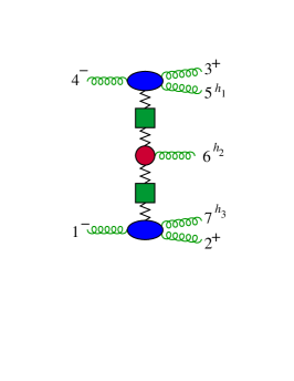
Figure 9: Factorization of the seven-gluon amplitude in planar ${\cal N}=4$ SYM in the $2\to 5$ multi-Regge limit. The additional factor not present in the six-point case is the central emission vertex (red blob), which again represents all orders. Again the vertical Regge cuts are omitted.

Dual conformal invariance implies that there are only $3\times 7-15=6$ independent variables for the seven-point remainder function. There are seven different dual conformal cross ratios,

$$u_{1} = \frac{s_{34}s_{671}}{s_{234}s_{345}}\,,\qquad u_{2}=\frac{s_{45}s_{712}}{s_{345}s_{456}}\,,\qquad u_{3}=\frac{s_{56}s_{123}}{s_{456}s_{567}}\,,\qquad u_{4}=\frac{s_{67}s_{234}}{s_{567}s_{671}}\,,$$

$$u_{5} = \frac{s_{71}s_{345}}{s_{671}s_{712}}\,,\qquad u_{6}=\frac{s_{12}s_{456}}{s_{712}s_{123}}\,,\qquad u_{7}=\frac{s_{23}s_{567}}{s_{123}s_{234}}\,,$$ (187)

with one nonlinear Gram determinant relation between them. In MRK, they behave as

$$u_{1}\,,u_{2}\,,u_{5}\,,u_{6}\sim{\cal O}(\delta),\qquad 1-u_{3}\,,1-u_{4}\sim{\cal O}(\delta),\qquad 1-u_{7}\sim{\cal O}(\delta^{2})\,,$$ (188)

where $\delta\to 0$, and the small ratios $p_{i+1}^{+}/p_{i}^{+}$ in eq. (185) are all ${\cal O}(\delta)$, for $i=4,5,6,7$.

This limit, which is to be taken after the analytical continuation

$$u_{7}\to u_{7}e^{-2\pi i}\,,$$ (189)

can be parametrized by two small real parameters $\tau_{1,2}$ and two complex variables $z_{1,2}$:

$$\sqrt{u_{1}u_{2}} = \tau_{1}\,,\qquad\frac{u_{1}}{1-u_{3}}=\left|\frac{1}{1-z_{1}}\right|^{2},\qquad\frac{u_{2}}{1-u_{3}}=\left|\frac{z_{1}}{1-z_{1}}\right|^{2},$$

$$\sqrt{u_{5}u_{6}} = \tau_{2}\,,\qquad\frac{u_{5}}{1-u_{4}}=\left|\frac{1}{1-z_{2}}\right|^{2},\qquad\frac{u_{6}}{1-u_{4}}=\left|\frac{z_{2}}{1-z_{2}}\right|^{2}.$$ (190)

The simplicial coordinates $\rho_{1},\rho_{2}$ are also used [192, 56]; they are related to $z_{1},z_{2}$ by

$$z_{1}=\frac{\rho_{1}(1-\rho_{2})}{\rho_{1}-\rho_{2}}\,,\qquad z_{2}=\frac{\rho_{2}-\rho_{1}}{1-\rho_{1}}\,.$$ (191)

There are 42 letters in the heptagon function symbol alphabet [193, 97]. In MRK they collapse to

$${\cal S}_{\rm hept,MRK}=\{\tau_{1,2}\,,\rho_{1,2}\,,1-\rho_{1,2}\,,\rho_{1}-\rho_{2}\,,\bar{\rho}_{1,2}\,,1-\bar{\rho}_{1,2}\,,\bar{\rho}_{1}-\bar{\rho}_{2}\}\,.$$ (192)

In analogy to the six-point case, the parity-even letters only involve $\tau_{1,2}$ and the five magnitudes,

$$\{|\rho_{1,2}|^{2}\,,|1-\rho_{1,2}|^{2}\,,|\rho_{1}-\rho_{2}|^{2}\}\,.$$ (193)

Only these parity-even combinations appear at the front of symbols, even after clipping off multiple $u_{7}$ initial entries [100], in accordance with the continuation (189). Therefore the relevant function space is SVHPLs in two variables, $\rho_{1}$ and $\rho_{2}$ [89, 56]. (In ref. [56] it has been argued that single-valued functions in multiple variables are all that is needed for MRK for any $n$-point amplitudes, at least at LL.)

An all-orders formula for the multi-Regge limit of any $n$-point amplitude in planar ${\cal N}=4$ SYM has been proposed based on some of the same ingredients encountered at $n=6$, plus a new ingredient, the central emission vertex [57]. The formula for $n=7$ is

$${\cal R}_{h_{1},h_{2},h_{3}}\,e^{i\delta_{7}} = 1+2\pi i\,\prod_{k=1,2}\left[\sum_{m_{k}=-\infty}^{\infty}\left(\frac{z_{k}}{\bar{z}_{k}}\right)^{\frac{m_{k}}{2}}\int_{\mathcal{C}_{k}}\frac{d\nu_{k}}{2\pi}|z_{k}|^{2i\nu_{k}}\tilde{\Phi}(\nu_{k},m_{k})e^{-(\ln\tau_{k}+i\pi)\omega(\nu_{k},m_{k})}\right]$$ (194)

$$\hbox{}\times\bigg{[}I^{h_{1}}(\nu_{1},m_{1})\cdot\tilde{C}^{h_{2}}(\nu_{1},m_{1},\nu_{2},m_{2})\cdot\bar{I}^{h_{3}}(\nu_{2},m_{2})\bigg{]}\,.$$

Here ${\cal R}_{h_{1},h_{2},h_{3}}$ is the appropriate helicity amplitude, divided by $A_{7}^{\rm BDS}$. The seven-point BDS phase is

$$\delta_{7}\ =\ \pi\Gamma\ln\left|\frac{\rho_{1}}{(1-\rho_{1})(1-\rho_{2})}\right|^{2}\,.$$ (195)

The quantity $\tilde{\Phi}(\nu,m)\equiv g^{2}\Phi_{\textrm{reg}}(\nu,m)/(\nu^{2}+m^{2}/4)$; $I^{h}$ is the helicity flip kernel (related to $\bar{H}$); and $\tilde{C}^{h}$ is the central emission vertex, whose all-orders expression is given in ref. [96], along with details about performing the $\nu_{k}$ integration. Note that $\tilde{\Phi}$ ($\tilde{C}^{h}$) does not correspond precisely to the blue (red) blob in fig. 9, since there are $n-5$ $\tilde{\Phi}_{r}$’s and only two true impact factors for any $n$. However, it is possible to associate a “square-root” of each $\tilde{\Phi}_{r}$ with a neighboring $\tilde{C}^{h}$ if one wants to make the correspondence more exact.

As mentioned in the introduction, seven-point amplitudes have been bootstrapped through four loops at the symbol level [97, 98, 99], and more recently at the level of full functions [101], by fixing zeta-valued constants of integration in the Euclidean region. The proposal (194) was checked first at symbol level [57], and more recently at function level, for both MHV and NMHV configurations, by carrying the constants of integration along a multi-step path from the Euclidean region to the $2\to 5$ multi-Regge limit [100].

4 Conclusions and Outlook

In this chapter, we have reviewed the behavior of amplitudes in QCD and in ${\cal N}=4$ SYM in the multi-Regge limit. In sec. 2, we have detailed how at LL and NLL accuracy QCD amplitudes are dominated by single-Reggeized-gluon exchange. At NNLL accuracy, three-Reggeized-gluon exchange occurs in the $2\to 2$ amplitude, starting at two loops. In the two-loop five-point amplitude, the central-emission vertex may couple to the three Reggeized gluons. It would be interesting to understand how that comes about, perhaps first in the context of full-color ${\cal N}=4$ SYM [53]. The three-Reggeized-gluon exchange yields a violation of Regge factorization only at the level of terms that are subleading in $N_{c}$. Basically, multi-Reggeon contributions seem to be washed away by the large $N_{c}$ limit. It is conceivable then that radiative corrections might be resummable in QCD through a BFKL equation at NNLL, at least in the large $N_{c}$ limit. Indeed, in planar ${\cal N}=4$ SYM the color-singlet BFKL eigenvalue has recently been obtained through NNNLL using quantum spectral curve methods [194, 195].

In sec. 3, we have analyzed the multi-Regge limit of amplitudes with six or more points in planar ${\cal N}=4$ SYM, in the long Regge cut configuration, characterized by an energy-sign flip of all the gluons emitted along the gluon ladder, which amounts to all the produced gluons except the first and the last in the strong rapidity ordering. The energy configuration of the outgoing gluons is then $(+,-,-,+)$ at six points, $(+,-,-,-,+)$ at seven points, and so forth. In this configuration, the amplitudes feature a two-Reggeized-gluon exchange [73, 74], and are conjecturally known for any leg multiplicity and at any logarithmic accuracy [57].

In the integrability picture of ${\cal N}=4$ SYM in the large $N_{c}$ limit in MRK [156], amplitudes which feature the exchange of an $n$-Reggeized-gluon ladder are related to an $n$-site Hamiltonian of an integrable spin chain. The amplitudes with exchange of a two-Reggeized-gluon ladder have been described in sec. 3. The two-site Hamiltonian is the BFKL Hamiltonian [196]. Therefore, those aspects of the integrability picture are non-trivially probed with the exchange of three or more Reggeized gluons. According to the integrability picture, amplitudes with eight or more points feature the exchange of a three-Reggeized-gluon ladder in the energy configuration characterized by a further energy-sign flip of the innermost gluons emitted along the gluon ladder [197]. The energy configuration of the outgoing gluons is then $(+,-,+,+,-,+)$ at eight points, $(+,-,+,+,+,-,+)$ at nine points, and so on. These contributions should have double discontinuities in the same channel, associated with pairs of vertical cuts. The exchange of a four-Reggeized-gluon ladder (associated with triple discontinuities) would appear in amplitudes with ten or more points featuring a further energy-sign flip of the innermost gluons, such that the energy configuration would be $(+,-,+,-,-,+,-,+)$ at ten points, $(+,-,+,-,-,-,+,-,+)$ at eleven points. One can continue flipping energies and considering more Reggeized gluons being exchanged.

Amplitudes at the two-loop level and up to nine points have been analyzed by lifting the symbol of ref. [102] to function level in the multi-Regge limit. For the regions $(+,-,+,+,-,+)$ and $(+,-,+,+,+,-,+)$ at eight and nine points, respectively, results are consistent with the picture of an amplitude made from impact factors and a central-emission vertex involving the exchange of a three-Reggeized-gluon ladder [105]. That is a good start for Lipatov’s integrability picture [156]. Much more, though, remains to be understood.

There are many other avenues for future research on the multi-Regge limit of gauge theory. They include further developments at NNLL in QCD, including also computations of impact factors and developments in the phenomenological application of these results (which we have not been able to review here). Beyond the planar limit, ${\cal N}=4$ SYM may provide a useful testing ground for untangling multi-Reggeized-gluon ladders from each other. Within the planar limit, MRK can serve as a window into the complexity of multi-loop $n$-point amplitudes for generic kinematics: the elliptic polylogarithms and more complicated functions that are expected to be encountered there must simplify drastically in MRK. Exactly how this works remains to be understood. All in all, the study of the multi-Regge limit in gauge theory will undoubtedly continue to be a rich mother lode within the field of scattering amplitudes.

References

- [1] Regge T 1959 Nuovo Cim. 14 951
- [2] Gribov V N and Pomeranchuk I Y 1962 Sov. Phys. JETP 15 788L
- [3] Gell-Mann M and Goldberger M L 1962 Phys. Rev. Lett. 9 275–277
- [4] Mandelstam S 1965 Phys. Rev. 137 B949–B954
- [5] Grisaru M T, Schnitzer H J and Tsao H S 1973 Phys. Rev. Lett. 30 811–814
- [6] Grisaru M T, Schnitzer H J and Tsao H S 1973 Phys. Rev. D 8 4498–4509
- [7] Gribov V N 1961 Zh. Eksp. Teor. Fiz. 41 1962
- [8] Chew G F and Frautschi S C 1961 Phys. Rev. Lett. 7 394–397
- [9] Cheng H and Wu T T 1970 Phys. Rev. D 1 2775–2794
- [10] Gribov V N, Lipatov L N and Frolov G V 1970 Yad. Fiz. 12 994
- [11] Lipatov L N 1976 Sov. J. Nucl. Phys. 23 338–345 [Yad. Fiz.23,642(1976)]
- [12] Fadin V S, Kuraev E A and Lipatov L N 1975 Phys. Lett. B60 50–52
- [13] Kuraev E A, Lipatov L N and Fadin V S 1976 Sov. Phys. JETP 44 443–450 [Zh. Eksp. Teor. Fiz.71,840(1976)]
- [14] Kuraev E A, Lipatov L N and Fadin V S 1977 Sov. Phys. JETP 45 199–204 [Zh. Eksp. Teor. Fiz.72,377(1977)]
- [15] Balitsky I I and Lipatov L N 1978 Sov. J. Nucl. Phys. 28 822–829 [Yad. Fiz.28,1597(1978)]
- [16] Fadin V S and Lipatov L N 1998 Phys. Lett. B429 127–134 (Preprint hep-ph/9802290)
- [17] Ciafaloni M and Camici G 1998 Phys. Lett. B430 349–354 (Preprint hep-ph/9803389)
- [18] Kotikov A V and Lipatov L N 2000 Nucl. Phys. B582 19–43 (Preprint hep-ph/0004008)
- [19] Kotikov A V and Lipatov L N 2003 Nucl. Phys. B661 19–61 [Erratum: Nucl. Phys.B685,405(2004)] (Preprint hep-ph/0208220)
- [20] Fadin V S and Lipatov L N 1989 JETP Lett. 49 352
- [21] Del Duca V 1996 Phys. Rev. D 54 989–1009 (Preprint hep-ph/9601211)
- [22] Fadin V S and Lipatov L N 1996 Nucl. Phys. B 477 767–808 (Preprint hep-ph/9602287)
- [23] Del Duca V 1996 Phys. Rev. D 54 4474–4482 (Preprint hep-ph/9604250)
- [24] Del Duca V 1996 Frascati Phys. Ser. 5 463–478 (Preprint hep-ph/9605404)
- [25] Fadin V S and Lipatov L N 1993 Nucl. Phys. B 406 259–292
- [26] Fadin V S, Fiore R and Quartarolo A 1994 Phys. Rev. D 50 5893–5901 (Preprint hep-th/9405127)
- [27] Fadin V S, Fiore R and Kotsky M I 1996 Phys. Lett. B 389 737–741 (Preprint hep-ph/9608229)
- [28] Del Duca V and Schmidt C R 1999 Phys. Rev. D 59 074004 (Preprint hep-ph/9810215)
- [29] Bern Z, Del Duca V and Schmidt C R 1998 Phys. Lett. B 445 168–177 (Preprint hep-ph/9810409)
- [30] Fadin V S, Fiore R, Kozlov M G and Reznichenko A V 2006 Phys. Lett. B639 74–81 (Preprint hep-ph/0602006)
- [31] Fadin V S, Kozlov M G and Reznichenko A V 2015 Phys. Rev. D92 085044 (Preprint 1507.00823)
- [32] Del Duca V and Glover E W N 2001 JHEP 10 035 (Preprint hep-ph/0109028)
- [33] Del Duca V, Duhr C, Gardi E, Magnea L and White C D 2012 Phys. Rev. D 85 071104 (Preprint 1108.5947)
- [34] Del Duca V, Duhr C, Gardi E, Magnea L and White C D 2011 JHEP 12 021 (Preprint 1109.3581)
- [35] Del Duca V, Falcioni G, Magnea L and Vernazza L 2014 Phys. Lett. B 732 233–240 (Preprint 1311.0304)
- [36] Del Duca V, Falcioni G, Magnea L and Vernazza L 2015 JHEP 02 029 (Preprint 1409.8330)
- [37] Fadin V S 2017 AIP Conf. Proc. 1819 060003 (Preprint 1612.04481)
- [38] Caron-Huot S, Gardi E and Vernazza L 2017 JHEP 06 016 (Preprint 1701.05241)
- [39] Fadin V S and Lipatov L N 2018 Eur. Phys. J. C 78 439 (Preprint 1712.09805)
- [40] Falcioni G, Gardi E, Milloy C and Vernazza L 2021 Phys. Rev. D 103 L111501 (Preprint 2012.00613)
- [41] Falcioni G, Gardi E, Maher N, Milloy C and Vernazza L 2022 JHEP 03 053 (Preprint 2111.10664)
- [42] Falcioni G, Gardi E, Maher N, Milloy C and Vernazza L 2021 (Preprint 2112.11098)
- [43] Almelid O, Duhr C, Gardi E, McLeod A and White C D 2017 JHEP 09 073 (Preprint 1706.10162)
- [44] Caola F, Chakraborty A, Gambuti G, von Manteuffel A and Tancredi L 2021 (Preprint 2112.11097)
- [45] Del Duca V, Duhr C and Smirnov V A 2010 JHEP 03 099 (Preprint 0911.5332)
- [46] Del Duca V, Duhr C and Smirnov V A 2010 JHEP 05 084 (Preprint 1003.1702)
- [47] Dixon L J, Drummond J M and Henn J M 2011 JHEP 1111 023 (Preprint 1108.4461)
- [48] Dixon L J, Drummond J M, von Hippel M and Pennington J 2013 JHEP 1312 049 (Preprint 1308.2276)
- [49] Dixon L J and von Hippel M 2014 JHEP 1410 65 (Preprint 1408.1505)
- [50] Henn J M and Mistlberger B 2016 Phys. Rev. Lett. 117 171601 (Preprint 1608.00850)
- [51] Caron-Huot S, Dixon L J, McLeod A and von Hippel M 2016 Phys. Rev. Lett. 117 241601 (Preprint 1609.00669)
- [52] Caron-Huot S, Dixon L J, Dulat F, von Hippel M, McLeod A J and Papathanasiou G 2019 JHEP 08 016 (Preprint 1903.10890)
- [53] Caron-Huot S, Chicherin D, Henn J, Zhang Y and Zoia S 2020 JHEP 10 188 (Preprint 2003.03120)
- [54] Dixon L J, Duhr C and Pennington J 2012 JHEP 10 074 (Preprint 1207.0186)
- [55] Basso B, Caron-Huot S and Sever A 2015 JHEP 01 027 (Preprint 1407.3766)
- [56] Del Duca V, Druc S, Drummond J, Duhr C, Dulat F, Marzucca R, Papathanasiou G and Verbeek B 2016 JHEP 08 152 (Preprint 1606.08807)
- [57] Del Duca V, Druc S, Drummond J M, Duhr C, Dulat F, Marzucca R, Papathanasiou G and Verbeek B 2020 Phys. Rev. Lett. 124 161602 (Preprint 1912.00188)
- [58] Caron-Huot S, Gardi E, Reichel J and Vernazza L 2020 JHEP 08 116 (Preprint 2006.01267)
- [59] Del Duca V, Dixon L J, Duhr C and Pennington J 2014 JHEP 02 086 (Preprint 1309.6647)
- [60] Del Duca V, Duhr C, Marzucca R and Verbeek B 2017 JHEP 10 001 (Preprint 1705.10163)
- [61] Rothstein I Z and Stewart I W 2016 JHEP 08 025 (Preprint 1601.04695)
- [62] Moult I, Solon M P, Stewart I W and Vita G 2018 JHEP 02 134 (Preprint 1709.09174)
- [63] Drummond J M, Henn J, Smirnov V A and Sokatchev E 2007 JHEP 01 064 (Preprint hep-th/0607160)
- [64] Bern Z, Czakon M, Dixon L J, Kosower D A and Smirnov V A 2007 Phys. Rev. D 75 085010 (Preprint hep-th/0610248)
- [65] Alday L F and Maldacena J M 2007 JHEP 06 064 (Preprint 0705.0303)
- [66] Bern Z, Carrasco J J M, Johansson H and Kosower D A 2007 Phys. Rev. D 76 125020 (Preprint 0705.1864)
- [67] Drummond J M, Korchemsky G P and Sokatchev E 2008 Nucl. Phys. B 795 385–408 (Preprint 0707.0243)
- [68] Drummond J M, Henn J, Korchemsky G P and Sokatchev E 2008 Nucl. Phys. B 795 52–68 (Preprint 0709.2368)
- [69] Nguyen D, Spradlin M and Volovich A 2008 Phys. Rev. D 77 025018 (Preprint 0709.4665)
- [70] Bern Z, Dixon L J, Kosower D A, Roiban R, Spradlin M, Vergu C and Volovich A 2008 Phys. Rev. D 78 045007 (Preprint 0803.1465)
- [71] Drummond J M, Henn J, Korchemsky G P and Sokatchev E 2009 Nucl. Phys. B 815 142–173 (Preprint 0803.1466)
- [72] Bern Z, Dixon L J and Smirnov V A 2005 Phys. Rev. D 72 085001 (Preprint hep-th/0505205)
- [73] Bartels J, Lipatov L N and Sabio Vera A 2009 Phys. Rev. D 80 045002 (Preprint 0802.2065)
- [74] Bartels J, Lipatov L N and Sabio Vera A 2010 Eur. Phys. J. C 65 587–605 (Preprint 0807.0894)
- [75] Lipatov L N and Prygarin A 2011 Phys. Rev. D 83 125001 (Preprint 1011.2673)
- [76] Fadin V S and Lipatov L N 2012 Phys. Lett. B 706 470–476 (Preprint 1111.0782)
- [77] Bartels J, Lipatov L N and Prygarin A 2011 Phys. Lett. B 705 507–512 (Preprint 1012.3178)
- [78] Lipatov L, Prygarin A and Schnitzer H J 2013 JHEP 01 068 (Preprint 1205.0186)
- [79] Basso B, Sever A and Vieira P 2013 Phys. Rev. Lett. 111 091602 (Preprint 1303.1396)
- [80] Goncharov A B, Spradlin M, Vergu C and Volovich A 2010 Phys. Rev. Lett. 105 151605 (Preprint 1006.5703)
- [81] Dixon L J, Drummond J M and Henn J M 2012 JHEP 01 024 (Preprint 1111.1704)
- [82] Caron-Huot S and He S 2012 JHEP 07 174 (Preprint 1112.1060)
- [83] Dixon L J, Drummond J M, Duhr C and Pennington J 2014 JHEP 06 116 (Preprint 1402.3300)
- [84] Dixon L J, von Hippel M and McLeod A J 2016 JHEP 01 053 (Preprint 1509.08127)
- [85] Caron-Huot S, Dixon L J, Dulat F, Von Hippel M, McLeod A J and Papathanasiou G 2019 JHEP 09 061 (Preprint 1906.07116)
- [86] Papathanasiou G 2022 J. Phys. A 55 443006 (Preprint 2203.13016)
- [87] Travaglini G et al. 2022 J. Phys. A 55 443001 (Preprint 2203.13011)
- [88] Brown F C S 2004 C. R. Acad. Sci. Paris, Ser. I 338 527
- [89] Broedel J, Sprenger M and Torres Orjuela A 2017 Nucl. Phys. B 915 394–413 (Preprint 1606.08411)
- [90] Drummond J M and Papathanasiou G 2016 JHEP 02 185 (Preprint 1507.08982)
- [91] Broedel J and Sprenger M 2016 JHEP 05 055 (Preprint 1512.04963)
- [92] Dixon L J and Dulat F The Seven-Loop Six-Gluon NMHV Amplitude in Planar Super-Yang-Mills Theory to appear
- [93] Bartels J, Kormilitzin A, Lipatov L N and Prygarin A 2012 Phys. Rev. D 86 065026 (Preprint 1112.6366)
- [94] Bartels J, Kormilitzin A and Lipatov L 2014 Phys. Rev. D 89 065002 (Preprint 1311.2061)
- [95] Bartels J, Kormilitzin A and Lipatov L N 2015 Phys. Rev. D 91 045005 (Preprint 1411.2294)
- [96] Del Duca V, Druc S, Drummond J, Duhr C, Dulat F, Marzucca R, Papathanasiou G and Verbeek B 2018 JHEP 06 116 (Preprint 1801.10605)
- [97] Drummond J M, Papathanasiou G and Spradlin M 2015 JHEP 03 072 (Preprint 1412.3763)
- [98] Dixon L J, Drummond J, Harrington T, McLeod A J, Papathanasiou G and Spradlin M 2017 JHEP 02 137 (Preprint 1612.08976)
- [99] Drummond J, Foster J, Gürdoğan O and Papathanasiou G 2019 JHEP 03 087 (Preprint 1812.04640)
- [100] Dixon L J, Liu Y T and Miczajka J 2021 JHEP 12 218 (Preprint 2110.11388)
- [101] Dixon L J and Liu Y T 2020 JHEP 10 031 (Preprint 2007.12966)
- [102] Caron-Huot S 2011 JHEP 12 066 (Preprint 1105.5606)
- [103] Prygarin A, Spradlin M, Vergu C and Volovich A 2012 Phys. Rev. D 85 085019 (Preprint 1112.6365)
- [104] Bargheer T, Papathanasiou G and Schomerus V 2016 JHEP 05 012 (Preprint 1512.07620)
- [105] Del Duca V, Duhr C, Dulat F and Penante B 2019 JHEP 01 162 (Preprint 1811.10398)
- [106] Bartels J 2020 (Preprint 2005.08818)
- [107] Alday L F and Maldacena J 2009 JHEP 11 082 (Preprint 0904.0663)
- [108] Alday L F, Gaiotto D and Maldacena J 2011 JHEP 09 032 (Preprint 0911.4708)
- [109] Alday L F, Maldacena J, Sever A and Vieira P 2010 J. Phys. A 43 485401 (Preprint 1002.2459)
- [110] Bartels J, Kotanski J and Schomerus V 2011 JHEP 01 096 (Preprint 1009.3938)
- [111] Bartels J, Schomerus V and Sprenger M 2012 JHEP 11 145 (Preprint 1207.4204)
- [112] Bartels J, Kotanski J, Schomerus V and Sprenger M 2013 (Preprint 1311.1512)
- [113] Bartels J, Schomerus V and Sprenger M 2014 JHEP 10 067 (Preprint 1405.3658)
- [114] Bartels J, Schomerus V and Sprenger M 2015 JHEP 07 098 (Preprint 1411.2594)
- [115] Sprenger M 2017 JHEP 01 035 (Preprint 1610.07640)
- [116] Abl T and Sprenger M 2022 JHEP 01 021 (Preprint 2108.02302)
- [117] Del Duca V 1995 Phys. Rev. D 52 1527–1534 (Preprint hep-ph/9503340)
- [118] Fadin V S and Fiore R 1992 Phys. Lett. B 294 286–292
- [119] Del Duca V and Schmidt C R 1998 Phys. Rev. D 57 4069–4079 (Preprint hep-ph/9711309)
- [120] Korchemsky G P and Radyushkin A V 1986 Phys. Lett. B 171 459–467
- [121] Moch S, Vermaseren J A M and Vogt A 2004 Nucl. Phys. B 688 101–134 (Preprint hep-ph/0403192)
- [122] Lipatov L N 1991 Nucl. Phys. B 365 614–632
- [123] Del Duca V 1995 (Preprint hep-ph/9503226)
- [124] Del Duca V and Schmidt C R 1995 Phys. Rev. D 51 2150–2158 (Preprint hep-ph/9407359)
- [125] Mueller A H and Navelet H 1987 Nucl. Phys. B 282 727–744
- [126] Del Duca V and Schmidt C R 1994 Phys. Rev. D 49 4510–4516 (Preprint hep-ph/9311290)
- [127] Stirling W J 1994 Nucl. Phys. B 423 56–79 (Preprint hep-ph/9401266)
- [128] Schmidt C R 2001 Review of BFKL 5th International Symposium on Radiative Corrections: Applications of Quantum Field Theory to Phenomenology (Preprint hep-ph/0106181)
- [129] Schmidt C R 1997 Phys. Rev. Lett. 78 4531–4535 (Preprint hep-ph/9612454)
- [130] Orr L H and Stirling W J 1997 Phys. Rev. D 56 5875–5884 (Preprint hep-ph/9706529)
- [131] Andersen J R and Smillie J M 2011 JHEP 06 010 (Preprint 1101.5394)
- [132] Lipatov L N 1986 Sov. Phys. JETP 63 904–912 [Zh. Eksp. Teor. Fiz.90,1536(1986)]
- [133] Pennington J 2013 JHEP 01 059 (Preprint 1209.5357)
- [134] Fadin V S, Kotsky M I and Fiore R 1995 Phys. Lett. B 359 181–188
- [135] Fadin V S, Fiore R and Kotsky M I 1996 Phys. Lett. B 387 593–602 (Preprint hep-ph/9605357)
- [136] Fadin V S, Fiore R and Quartarolo A 1996 Phys. Rev. D 53 2729–2741 (Preprint hep-ph/9506432)
- [137] Blümlein, J and Ravindran, V and van Neerven, W L 1998 Phys. Rev. D 58 091502 (Preprint hep-ph/9806357)
- [138] Erdoğan O and Sterman G 2015 Phys. Rev. D 91 016003 (Preprint 1112.4564)
- [139] Falcioni G, Gardi E and Milloy C 2019 JHEP 11 100 (Preprint 1909.00697)
- [140] Korchemsky G P and Radyushkin A V 1987 Nucl. Phys. B283 342–364
- [141] Caron-Huot S 2018 JHEP 03 036 (Preprint 1501.03754)
- [142] Fadin V S, Fiore R and Quartarolo A 1994 Phys. Rev. D 50 2265–2276 (Preprint hep-ph/9310252)
- [143] Del Duca V 2018 JHEP 02 112 (Preprint 1712.07030)
- [144] Chirilli G A and Kovchegov Y V 2013 JHEP 06 055 (Preprint 1305.1924)
- [145] Chirilli G A and Kovchegov Y V 2014 JHEP 05 099 [Erratum: JHEP08,075(2015)] (Preprint 1403.3384)
- [146] Goncharov A B 1998 Math. Research Letters 5 497
- [147] Goncharov A B 2001 (Preprint math/0103059v4)
- [148] Remiddi E and Vermaseren J A M 2000 Int. J. Mod. Phys. A15 725–754 (Preprint hep-ph/9905237)
-
[149]
Brown F C S
http://www.ihes.fr/~brown/RHpaper5.pdf - [150] Brown F 2014 SIGMA 2 e25 (Preprint 1309.5309)
- [151] Brown F C S 2015 (Preprint 1512.06410)
- [152] Schnetz O 2016 (Preprint 1606.08598)
- [153] Kotikov A V, Lipatov L N and Velizhanin V N 2003 Phys. Lett. B557 114–120 (Preprint hep-ph/0301021)
- [154] Gadde A, Pomoni E and Rastelli L 2009 (Preprint 0912.4918)
- [155] Del Duca V, Marzucca R and Verbeek B 2022 JHEP 01 149 (Preprint 2111.14265)
- [156] Lipatov L N 2009 J. Phys. A 42 304020 (Preprint 0902.1444)
- [157] Del Duca V, Frizzo A and Maltoni F 2000 Nucl. Phys. B 568 211–262 (Preprint hep-ph/9909464)
- [158] Antonov E N, Lipatov L N, Kuraev E A and Cherednikov I O 2005 Nucl. Phys. B 721 111–135 (Preprint hep-ph/0411185)
- [159] Duhr C 2009 New techniques in QCD Ph.D. thesis Louvain U., CP3
- [160] Byrne E P, Del Duca V, Dixon L J, Gardi E and Smillie J M 2022 JHEP 08 271 (Preprint 2204.12459)
- [161] Mandelstam S 1983 Nucl. Phys. B 213 149–168
- [162] Brink L, Lindgren O and Nilsson B E W 1983 Phys. Lett. B 123 323–328
- [163] Howe P S, Stelle K S and Townsend P K 1984 Nucl. Phys. B 236 125–166
- [164] ’t Hooft G 1974 Nucl. Phys. B 72 461
- [165] Beisert N et al. 2012 Lett. Math. Phys. 99 3–32 (Preprint 1012.3982)
- [166] Brandhuber A, Heslop P and Travaglini G 2008 Nucl. Phys. B 794 231–243 (Preprint 0707.1153)
- [167] Drummond J M, Henn J, Korchemsky G P and Sokatchev E 2010 Nucl. Phys. B 826 337–364 (Preprint 0712.1223)
- [168] Alday L F and Roiban R 2008 Phys. Rept. 468 153–211 (Preprint 0807.1889)
- [169] Adamo T, Bullimore M, Mason L and Skinner D 2011 J. Phys. A 44 454008 (Preprint 1104.2890)
- [170] Beisert N, Eden B and Staudacher M 2007 J. Stat. Mech. 0701 P01021 (Preprint hep-th/0610251)
- [171] Alday L F, Gaiotto D, Maldacena J, Sever A and Vieira P 2011 JHEP 04 088 (Preprint 1006.2788)
- [172] Basso B 2012 Nucl. Phys. B 857 254–334 (Preprint 1010.5237)
- [173] Basso B, Sever A and Vieira P 2014 JHEP 01 008 (Preprint 1306.2058)
- [174] Basso B, Sever A and Vieira P 2014 JHEP 08 085 (Preprint 1402.3307)
- [175] Basso B, Sever A and Vieira P 2014 JHEP 09 149 (Preprint 1407.1736)
- [176] Parke S J and Taylor T R 1986 Phys. Rev. Lett. 56 2459
- [177] Bern Z, Dixon L J, Dunbar D C and Kosower D A 1994 Nucl. Phys. B425 217–260 (Preprint hep-ph/9403226)
- [178] Dixon L J 2018 JHEP 01 075 (Preprint 1712.07274)
- [179] Cachazo F, Spradlin M and Volovich A 2007 Phys. Rev. D 76 106004 (Preprint 0707.1903)
- [180] Agarwal B, von Manteuffel A, Panzer E and Schabinger R M 2021 Phys. Lett. B 820 136503 (Preprint 2102.09725)
- [181] Spradlin M, Volovich A and Wen C 2008 Phys. Rev. D 78 085025 (Preprint 0808.1054)
- [182] Duhr C 2015 Mathematical aspects of scattering amplitudes Theoretical Advanced Study Institute in Elementary Particle Physics: Journeys Through the Precision Frontier: Amplitudes for Colliders pp 419–476 (Preprint 1411.7538)
- [183] Caron-Huot S, Dixon L J, Drummond J M, Dulat F, Foster J, Gürdoğan O, von Hippel M, McLeod A J and Papathanasiou G 2020 PoS CORFU2019 003 (Preprint 2005.06735)
- [184] Gaiotto D, Maldacena J, Sever A and Vieira P 2011 JHEP 12 011 (Preprint 1102.0062)
- [185] Caron-Huot S 2015 JHEP 05 093 (Preprint 1309.6521)
- [186] Benna M K, Benvenuti S, Klebanov I R and Scardicchio A 2007 Phys. Rev. Lett. 98 131603 (Preprint hep-th/0611135)
- [187] Bartels J, Lipatov L N and Prygarin A 2011 (Preprint 1104.4709)
- [188] Georgiou G 2009 JHEP 09 021 (Preprint 0904.4675)
- [189] Dorn H and Wuttke S 2011 JHEP 05 114 (Preprint 1104.2469)
- [190] Dorn H and Wuttke S 2012 JHEP 04 023 (Preprint 1111.6815)
- [191] Dixon L J and Esterlis I 2016 JHEP 07 116 [Erratum: JHEP 08, 131 (2016)] (Preprint 1602.02107)
- [192] Brown F C S 2009 Annales Sci. Ecole Norm. Sup. 42 371 (Preprint math/0606419)
- [193] Golden J, Goncharov A B, Spradlin M, Vergu C and Volovich A 2014 JHEP 01 091 (Preprint 1305.1617)
- [194] Alfimov M, Gromov N and Sizov G 2018 JHEP 07 181 (Preprint 1802.06908)
- [195] Velizhanin V N 2021 (Preprint 2106.06527)
- [196] Lipatov L N 1993 Phys. Lett. B 309 394–396
- [197] Bartels J, Lipatov L N and Prygarin A 2011 J. Phys. A 44 454013 (Preprint 1104.0816)
- [198] Binosi D, Collins J, Kaufhold C and Theussl L 2009 Comput. Phys. Commun. 180 1709–1715 (Preprint 0811.4113)