The SAGEX Review on Scattering Amplitudes
Chapter 12: Amplitudes and collider physics

Abstract

We explore how various topics in modern scattering amplitudes research find application in the description of collider physics processes. After a brief review of experimentally measured quantities and how they are related to amplitudes, we summarise recent developments in perturbative QFT, and how they have impacted our ability to do precision physics with colliders. Next, we explain how the study of (next-to-)soft radiation is directly relevant to increasing theoretical precision for key processes at the LHC and related experiments. Finally, we describe the various techniques that are used to turn theoretical calculations into something more closely approaching the output of a particle accelerator.

• October 2021

1 Introduction

As the SAGEX network has made clear, the study of scattering amplitudes has become an extraordinarily broad endeavour. Theories studied range from well-established theories of nature (e.g. the Standard Model, plus effective field theory corrections) right through to highly supersymmetric versions of non-abelian gauge theories, or even string theories. The latter are less relevant for current experiments, but can be useful for developing new calculational techniques, or for showing up relationships between different types of theory. Furthermore, new mathematics is often needed in order to bring new aspects of field theory to light, such that dialogue between pure mathematicians and physicists has been an increasing facet of the amplitudes community in recent years. What makes this mix so important is that new techniques used to study more formal theories are very often the same techniques that have been used to generate highly non-trivial results in more physically relevant theories. However, the diversity of the amplitudes community can be as much of a hindrance as it is a strength: it becomes ever-more difficult for any given person – and especially a newcomer to the field – to see how different branches of amplitudes research are related, and to know how formal ideas in one corner are applied to very practical ends in another.

The aim of this article is to redress this balance somewhat, by focusing on one of the main motivations for studying amplitudes in the first place, namely that they underlie the physics of collider experiments. The latter form our main way of testing theories of fundamental physics, which itself is at a crucial crossroads. With the discovery of the Higgs boson in 2012, the SM is experimentally complete, but its obvious deficiencies cry out for a deeper explanation. The current flagship experiment is the Large Hadron Collider at CERN, which will be with us for at least another two decades. Replacement colliders are being actively considered, although the lack of any particularly striking new physics hints at the LHC make it rather unclear what the optimum follow-up machine will look like.

In order to make progress, we must continue to develop new types of collider, as well as our understanding of quantum field theory. On very general grounds, any new physics will look QFT-like at currently available collider energies. Furthermore, the lack of any very clear new physics means that we have to understand the old physics (i.e. the SM) extremely well. Only by knowing the old physics very very precisely can we be sure that tiny deviations we might see in experiments are genuine new physics, rather than poorly understood old physics. Furthermore, given that collider experiments involve scattering particles, it is the study of scattering amplitudes in QFT that is the most relevant thing to be doing.

Given that you are reading this article, I am assuming that you will already be familiar with what a scattering amplitude is, whether or not this is in our own apparently four-dimensional and distinctly non-conformal world. However, you may well not be familiar with what goes on inside a collider, what experimentalists do with it, and how you can start to turn a scattering amplitude into something they might be interested in. Although some of the ideas may well have already been presented to you in some region of your past light-cone, we review relevant material in the following sections.

2 What is a collider, and what does it measure?

A particle accelerator or collider is an experiment that accelerates one or more beams of particles so that they collide. Early versions of this idea had a single beam colliding with a fixed target, which is easier to build, but suffers from the fact that much of the energy in the initial state gets wasted as kinetic energy in the final state. Hence, for the past few decades, colliders have consisted of two beams of particles that collide in the centre-of-mass frame. Electric and magnetic fields are used to accelerate the particles and focus the beams, and thus the particles being accelerated must be (electromagnetically) charged. Recent examples include LEP ($e^{+}e^{-}$), the Tevatron ($p\bar{p}$), and the LHC ($pp$), where $e^{\pm}$ denotes the electron and positron, and $(p,\bar{p}$) the (anti-)proton. Colliders tend to be circular, which gives multiple chances to accelerate the particles each time they go around the ring. However, charged particles of energy $E$ and mass $m$ radiate synchrotron radiation at a rate $\propto(E/m)^{4}r^{-2}$, imposing a practical limit on how much we can accelerate them. This is why the most modern collider (the LHC) uses heavy particles (protons rather than electrons), and has a very large circumference of 27 km! Protons are not ideal – they are composite, wobbly bags of quarks and gluons. This makes hadron colliders messier than $e^{-}e^{+}$ colliders, making precision physics more difficult. Thus, future colliders may return to using electrons and positrons, at the expense of needing new technology for colliding them in a linear fashion.

The beams in a particle accelerator are focused so that they collide, which in modern circular colliders happens at multiple points around the ring. Each collision of the beam particles is referred to as a (scattering) event, and the aim of each experiment is to record and analyse interesting-looking events. The collision points are surrounded by a cylindrical detector, whose aim is to collect as many of the particles emerging from a collision point as possible. The detectors contain multiple layers for capturing different types of particle, and measuring their momenta and charges. Some particles, such as weakly-interacting neutrinos or possible new physics particles, pass through the detector and thus appear as “missing 4-momentum” (i.e. a failure of momentum conservation) in a given scattering event. From a very naïve theorist’s viewpoint, one may thus characterise individual scattering events by a recorded list of particles, together with their measured 4-momenta. We will return to how accurate this picture is in section 7, but for now let us note that in a quantum theory it is not possible to predict exactly which particles will emerge in any given event, nor what their precise momenta will be. Instead, we can only calculate probabilities for certain final states to appear in the detector, and then compare the measured properties of events with predicted distributions from a given QFT.

If we consider a simple classical scattering process, such as throwing tennis balls at a target, it is clear that the probability of hitting the target depends on its cross-sectional area. This is equally true of quantum scattering, for which the relevant cross-sectional area represents an effective range of interaction for particles incident on the target. It follows that the rate of scattering events for a given pair of incoming beams can be written as

$$\frac{dN}{dt}\propto\sigma,$$ (1)

where $N$ is the number of events, $t$ the time, and $\sigma$ has units of area. It is called the cross-section, and depends on the intrinsic properties of the incoming particles, thus is calculable from QFT. The quantity relating the two sides of eq. (1) is usually written ${\cal L}(t)$, as it may depend on time in general. It is called the luminosity and, roughly speaking, measures how the incoming particles are distributed within the beams i.e. how “bright” the beams are. Here we have been talking about the total number of scattering events, but we can choose to focus on a particular type of event e.g. those containing a pair of top quarks, or a single Higgs boson. Letting $N_{i}$ denote the number of events for distinct processes $\{i\}$, we have

$$N=\sum_{i}N_{i}\quad\Rightarrow\quad\frac{dN_{i}}{dt}={\cal L}(t)\sigma_{i},$$ (2)

where $\sigma_{i}$ is the cross-section for process $i$, such that the total cross-section for interaction is $\sigma=\sum_{i}\sigma_{i}$. It is not possible to think of each individual cross-section as a physical area, but we do not have to do this: eq. (2) tells us that the cross-section for a given process is simply given by the event rate, divided by the luminosity. Experimentalists measure the luminosity ${\cal L}(t)$, so that they can then present results for cross-sections directly, for comparison with theory. For historical reasons, the conventional unit of cross-section is the barn (b), where one barn is defined to be 10^-28m². For context, the total $pp$ cross-section at the LHC (at 13 TeV) is about 0.1b. The cross-section for single Higgs boson production in its main production mode (gluon-gluon fusion) is about 57pb (here the “p” stands for pico, or $10^{-12}$), which gives some indication of the huge range of cross-sections for interesting processes at the LHC, and how very tiny signals have to be extracted from a massive amount of other data. Given that the luminosity is related to the total event rate, it follows that the integrated luminosity

$$L(t)=\int_{0}^{t}dt^{\prime}{\cal L}(t^{\prime})$$

is a measure of the total number of events collected by a given collider after a time of operation $t$. From eq. (1) and the fact that the event number $N$ is dimensionless, the integrated luminosity has units of inverse area. As an example, the LHC delivered 156 fb^-1 (inverse femtobarns) of integrated luminosity during Run 2 at 13 TeV. Given the inverse units, a smaller prefix (nano, pico, femto) means more events have been collected.

3 Cross-sections and amplitudes

In the previous section, we have seen that a given scattering process $i$ has an associated cross-section $\sigma_{i}$. In principle, QFT tells us how to calculate this. Let us first consider the case that the incoming and outgoing particles are fundamental particles. Let $p_{1}$ and $p_{2}$ be the incoming particle momenta, and $\{p_{3},\ldots p_{n}\}$ the final momenta, so that there are $(n-2)$ particles in the final state. Then your QFT textbook will tell you that the cross-section can be decomposed into the following form:

$$\sigma_{i}=\frac{1}{F(p_{1},p_{2})}\int d\Phi^{(n-2)}(p_{3},\ldots,p_{n}){\cal A}_{i}(\{p_{i}\}).$$ (3)

Here

$$F(p_{1},p_{2})=4[(p_{1}\cdot p_{2})^{2}-m_{1}^{2}m_{2}^{2}]^{1/2},$$ (4)

where $m_{i}$ is the mass of beam particle $i$, is called the Lorentz-invariant flux. It is a convenient relativistic generalisation of the usual flux describing how the beam particles are moving relative to each other. There is also an integration over the momenta of the final state particles, given by the Lorentz-invariant phase space

$$\int d\Phi^{(n-2)}=(2\pi)^{4}\left(\prod_{i=1}^{n-2}\int\frac{d^{3}\vec{p}_{i}}{(2\pi)^{3}2E_{i}}\right)\delta^{(4)}(P_{\rm final}-P_{\rm init.}).$$ (5)

Here $E_{i}$ is the energy of particle $i$, and $\vec{p}_{i}$ its (relativistic) 3-momentum. Also, $P_{\rm init.}$ ($P_{\rm final}$) are the total 4-momentum in the initial (final) state respectively. We then see that the delta function in eq. (5) implements total momentum conservation in the scattering process. Finally in eq. (3), ${\cal A}_{i}$ is the scattering amplitude for process $i$, which the SAGEX collaboration was set up to investigate in a myriad of ways. Equation (3) suggests how you as a theorist might compare a given QFT with experiment: for a given process, you can calculate the appropriate scattering amplitude using perturbation theory, before integrating over the phase-space, and dividing by the appropriate flux factor. The resulting number may then be compared with something produced by experimentalists, if they have isolated the relevant events. The process might be a potential new physics process, and if the number agrees you may end up with an expenses-paid trip to Stockholm. Or it might be a process that occurs in the Standard Model, so that your number allows an experimentalist to efficiently disentangle new from old physics, so that they might go to Stockholm.

Total cross-sections are a very crude way of comparing theory with data. It is also possible to compare differential cross-sections, where one does not integrate over the full phase space in eq. (3). Given an observable ${\cal O}$, the quantity $(d\sigma_{i}/d{\cal O})$ represents the distribution of ${\cal O}$ as measured in events collected in scattering process $i$. Experimentalists often normalise this by dividing by the total cross-section, given that many uncertainties cancel out when doing this. An example distribution is shown in figure 1, which comes from an analysis of events containing (anti-)top quark pairs by the ATLAS experiment [1]. The (anti-)top quarks decay to produce leptons, and the collaboration have measured the azimuthal angle in the detector between these decay products, where the data is compared to various predictions from theorists. Interestingly, the theory curves do not agree with the data particularly well by eye. Statistically, however, there is no cause for excitement: the lower panel depicts the uncertainty on the measurement as a grey band, which indeed overlaps with the (Standard Model) theory.

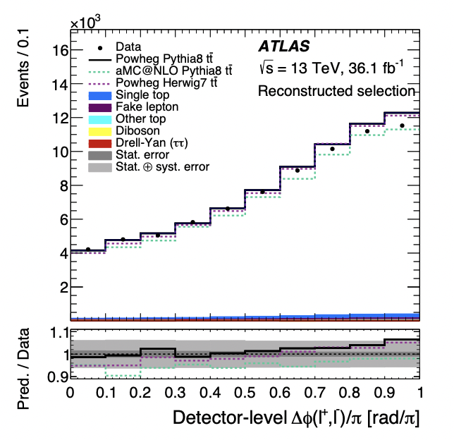
Figure 1: Distribution of the azimuthal angle between leptons originating from top quark decays. From ref. [1].

It goes almost without saying that the above discussion is vastly oversimplified. The comparison of theory with data is, in practice, almost nothing like the simple procedure outlined here. Typical complications include the following:

• Amplitudes in QFT suffer from ultraviolet (UV) divergences at loop-level. These can be dealt with via renormalisation in some scheme, and modern-day theorists typically use dimensional regularisation in $4-2\epsilon$ dimensions. Then cross-sections for comparison with experiment will depend on the renormalisation scale $\mu_{R}$. In particular, the QCD expansion parameter will become a running coupling $\alpha_{s}(\mu_{R})$. The coefficients of the perturbation expansion in this parameter involve large logarithms involving ratios of $\mu_{R}$ with energy scales typical of the scattering process (e.g. invariants formed from the particle momenta). Thus, dependence on $\mu_{R}$ is minimised at a given order in perturbation theory by choosing $\mu_{R}$ to be comparable with these energy scales.

• The incoming particles at the LHC are protons, which are not fundamental particles in QCD, and thus not fully described by standard perturbation theory. We must then generalise the formula of eq. (3), given that we can calculate scattering amplitudes in perturbation theory for incoming (anti-)quarks and / or gluons, but not protons. We discuss this in section 4.

• We can typically only calculate the amplitude to low orders in perturbation theory, where the strong interaction (with expansion parameter $\alpha_{s}\equiv g_{s}^{2}/(4\pi)$, where $g_{s}$ is the QCD coupling constant) is the most relevant. The state of the art for many processes of interest is next-to-leading order (NLO) in $\alpha_{s}$, although NNLO is known for some cases. Some cross-sections are known to a highly impressive N³LO! Examples include different production modes for the Higgs boson [2, 3, 4, 5], and the so-called Drell-Yan production of a heavy particle [6], which we will see in more detail below. Proceeding order-by-order in the coupling in this way is known as fixed-order perturbation theory, and we discuss this in section 5.

• Perturbation theory can be unstable: for differential cross-sections, the coefficients of the perturbation series depend on the external particle momenta, and can diverge in certain kinematic regions (such as the soft limit, in which the 4-momentum of emitted radiation goes to zero). One must then sum up certain contributions to all orders in perturbation theory for meaningful comparison with data, a process known as resummation, discussed in section 6.

• Real scattering events contain huge numbers of quarks and gluons, going way beyond what a perturbative QCD calculation can achieve. One must therefore estimate the effect of this additional radiation using well-motivated QFT-based arguments. We return to this in section 7.

• Real scattering events do not contain free (anti-)quarks and gluons, due to the confinement property of QCD. They instead contain hadrons, and we must try and estimate how. This is also discussed in section 7.

This list – which is not even complete – is enough to scare off any theorist who hopes that their research on scattering amplitudes might have something to say about experiments. Let us thus retreat to the relative safety of eq. (3), and get gradually closer to what happens at the LHC.

4 Cross-sections at hadron colliders

The first thing we have to deal with is the issue of incoming protons. At first glance, one might think that we could never calculate cross-sections with incoming protons, given that – with a few exceptions in special circumstances or theories – we only really know how to calculate amplitudes using perturbation theory. However, what saves us is the well-known property of asymptotic freedom [7, 8], according to which the QCD expansion parameter $\alpha_{s}(\mu_{R})$ becomes weaker with increasing renormalisation scale $\mu_{R}$. Given that this is identified with a typical energy scale $Q$ in the scattering process of interest, we find that highly energetic protons will contain approximately free (anti-)quarks and gluons. We can indeed calculate a perturbative cross-section for the latter, and may then combine it with appropriate distribution functions measuring how the (anti-)quarks are distributed within the proton, in order to describe the total proton-proton cross-section. This was first formulated by Feynman [9, 10], who called it the parton model. At that time, partons were stipulated as hypothetical elementary constituents of the proton, and were only later realised to be the (anti-)quarks and gluons of QCD. The word “parton”, however, is still in use, as it is very convenient to have a single word that can be used to denote any (anti-)quark or gluon!

More precisely, consider partons that emerge from the incoming protons, where the latter can be taken to have momenta $P_{1}$ and $P_{2}$. If the protons are very fast-moving, the emerging partons will have momenta $\{p_{i}\}$ that are approximately collinear with the $\{P_{i}\}$, and which may thus be written as

$$p_{i}=x_{i}P_{i},\quad 0\leq x_{i}\leq 1,$$ (6)

where no summation is implied on the right-hand side, and where $x_{i}$ represents the (longitudinal) momentum fraction of parton $i$. The hadronic cross-section for a given process may then be written as 

$$\sigma=\sum_{i,j\in\{q,\bar{q},g\}}\int_{0}^{1}dx_{1}\int_{0}^{1}dx_{2}\,f_{i}(x_{1})f_{j}(x_{2})\hat{\sigma}_{ij}(\{p_{i}\},\mu_{R}).$$ (7)

Here $\hat{\sigma}_{ij}$ denotes the partonic cross-section, for incoming (anti-)quarks and gluons. The quantity $f_{i}(x_{j})$ is a parton distribution function (PDF), that represents, loosely speaking, the probability to find a parton with momentum fraction $x_{j}$ inside incoming proton $i$. We must then sum over all possible momentum fractions, and over all possible species of parton, including over all possible flavours of quark $q$ and their anti-particles. The latter might surprise you if you are familiar only with the conventional undergraduate wisdom that protons contain two up quarks and a down quark. Needless to say, this statement is not to be taken too literally: in quantum field theory, partons are constantly popping in and out of the vacuum due to virtual effects, so that the proton is some sort of localised collection of quantum partonic froth, whose net quantum numbers are the same as two up quarks and a down quark! Whilst the partonic cross-section $\hat{\sigma}_{ij}$ is calculable in perturbation theory, the parton distribution functions $\{f_{i}\}$ are not. They can, however, be measured from experiment, and used to predict the results of subsequent experiments.

You may be wondering if the parton model can be rigorously justified from first-principles QFT, where the relevant field theory is QCD in this case. Indeed it can for certain scattering processes, using the operator product expansion (see e.g. ref. [11] for a textbook treatment). More simply, we might ask what goes wrong if we were to ignore eq. (7), and try to use perturbation theory to describe QCD scattering. At leading order (LO) in $\alpha_{s}$, everything is well-behaved. However, at NLO and beyond, problems occur due to emitting additional radiation from either incoming or outgoing partons. An example is shown in figure 2 which, using Feynman rules (or otherwise) results in an extra factor in the scattering amplitude for a given process

$$\frac{1}{(p_{1}-k)^{2}}=\frac{1}{-2p_{1}\cdot k}=\frac{1}{-2|\vec{p}_{1}||\vec{k}|(1-\cos\theta)},$$ (8)

where 4-momenta are labelled as in the figure, and we neglect the mass of the incoming quark, given that this is negligible at all relevant collider energies (at least for the up and down quarks). We have also introduced the 3-momenta of the quark and gluon, $\vec{p}_{1}$ and $\vec{k}$, as well as the angle $\theta$ between them. Clearly the additional factor of eq. (8) diverges in two cases: (i) the additional radiation is soft ($|\vec{k}|\rightarrow 0$); (ii) the additional radiation is collinear with the emitting particle ($\theta\rightarrow 0$). Furthermore, these cases are not mutually exclusive: the radiation may be soft and collinear, which is even more divergent! These are known as infrared (IR) divergences, to distinguish them from the UV divergences encountered above. Although we considered the example of real radiation here, the virtual (loop) corrections to the amplitude are also IR-divergent, and the solution to this problem is well-known. First, one must be careful to consider only those cross-sections and related observables that are infrared-safe, meaning that the definition is robust under the inclusion of additional soft and / or collinear radiation. For example, the cross-section for a single Higgs boson accompanied by any amount of QCD radiation is IR-safe, whereas the cross-section for a Higgs boson plus exactly three detected gluons is not. Once we have chosen an IR-safe observable, the divergences are guaranteed to cancel in QED by the Bloch-Nordsieck theorem [12], if we add together all virtual and real contributions at any given order in perturbation theory. In QCD, the KLN theorem [13, 14] theorem states that this cancellation will only occur if we include initial states containing arbitrary numbers of incoming particles, which is inconvenient for describing scattering processes with two incoming beams. Instead requiring only two incoming particles leads to cancellation of all soft singularities, together with collinear singularities associated with the outgoing particles in the final state. However, one is left with uncancelled collinear singularities associated with the two incoming particles, which potentially pose a serious problem.

What saves us is the presence of the parton distributions $\{f_{i}\}$ in eq. (7). We are clearly free to redefine both the partons and the partonic cross-section such that eq. (7) remains invariant. Thus, we can choose to remove collinear divergences from the partonic cross-section by absorbing them into the parton distributions. In other words, one replaces the bare parton distributions appearing in eq. (7) with modified ones, chosen so that singularities in the partonic cross-section are removed. One way to do this is simply to dictate that all radiation below a particular factorisation scale $\mu_{F}$ is reabsorbed into a redefined parton distribution, so that it is absent from the partonic cross-section. However, this procedure is typically not used in practical calculations, given that applying momentum cut-offs is not gauge invariant. Instead, dimensional regularisation is often used in $d=4-2\epsilon$ dimensions, in which IR divergences show up as poles in $\epsilon$. The factorisation scale then emerges through the additional scale $\mu$ that is introduced to keep the coupling dimensionless. A particular means of removing divergences from the partonic cross-section is called a factorisation scheme and, whilst the partonic cross-section becomes finite, the calculated parton distributions are not. This is not a problem: we do not claim to be able to calculate the partons in perturbation theory, and so instead can simply measure them from experiment. Indeed, this is reminiscent with what happens when we remove UV singularities via renormalisation: in doing so, we lose the ability to calculate the coupling constant, which instead becomes a measurable parameter in some given scheme.

Figure 2: Gluon radiation from an incoming quark leg.

The upshot of the above discussion is that eq. (9) gets replaced by the more general formula

$$\sigma =\sum_{i,j\in\{q,\bar{q},g\}}\int_{0}^{1}dx_{1}\int_{0}^{1}dx_{2}\,f_{i}(x_{1},\mu_{F})f_{j}(x_{2},\mu_{F})\hat{\sigma}_{ij}(\{p_{i}\},\mu_{R},\mu_{F})$$ (9)

$$\quad+{\cal O}\left(\frac{\Lambda^{2}}{Q^{2}}\right).$$

That is, both the partons and partonic cross-section now depend on the factorisation scale $\mu_{F}$, which typically enters through dimensionless ratios involving an energy scale $Q$ associated with the scattering process. As for the renormalisation scale $\mu_{R}$, dependence on $\mu_{F}$ cancels at a given order in perturbation theory, but there can be a residual dependence associated with missing higher-order corrections, and this takes the form of logarithms of ratios of the factorisation scale with typical energy scales involved in the scattering process. As for the case of $\mu_{R}$ above, one can reduce this dependence by choosing $\mu_{F}$ to be such a typical energy scale $Q$, and there is clearly some ambiguity in this choice. Varying $\mu_{R}$ and $\mu_{F}$ around some default value then gives a measure of the theoretical uncertainty of a given cross-section prediction. We have also noted in eq. (9) that the parton model formula receives formal corrections when derived from first-principles QFT, involving ratios of the QCD confinement scale $\Lambda$ and the typical energy scale $Q$. Provided that $Q$ is large enough that we trust perturbation theory in the first place, these so-called power corrections will be small.

5 Fixed-order perturbation theory

So far the job of a theorist seems clear enough: to compare theory to data at a hadron collider such as the LHC, we must calculate amplitudes involving incoming partons (i.e. (anti-)quarks and gluons), turn these into partonic cross-sections using eq. (3), and then combine these with parton distributions using one of the many versions of these which are available (see e.g. refs. [15, 16, 17, 18] for recent analyses). However, anyone who has tried to calculate scattering amplitudes for relevant scattering processes knows that this becomes extraordinarily difficult as the number of loops or number of legs increases. Traditionally, QCD amplitudes were calculated using Feynman rules and diagrams, which represent the $L$-loop amplitude as a sum of integrals of the form

$${\cal A}^{(L)}(\{p_{i}\})=\sum_{{\rm diags}\,\,j}\left(\prod_{k=1}^{L}\int\frac{d^{d}l_{k}}{(2\pi)^{d}}\right)\frac{c_{j}\,{\cal N}_{j}(\{p_{i}\},\{l_{k}\})}{{\cal D}_{j}(\{p_{i}\},\{l_{k}\})}.$$ (10)

Here each individual diagram $j$ has a colour factor $c_{j}$, and integrals over the $L$ loop momenta $\{l_{k}\}$. There is then a kinematic numerator ${\cal N}_{j}$ and denominator ${\cal D}_{j}$, each of which depends on both the external momenta $\{p_{i}\}$ and loop momenta $\{l_{k}\}$ in general. Terms in the integrand with zero, one or more than one powers of loop momenta in the numerator are referred to as scalar, vector or tensor integrals respectively, and it is in fact possible to apply algebraic identities to reduce all higher-rank integrals to scalar ones. This may be formalised in a process known as Passarino-Veltman reduction [19], which may be automated in principle, albeit with some subtle caveats for higher-leg processes. Then, all $L$-loop amplitudes can in principle be straightforwardly calculated once a suitable basis for all $L$-loop scalar integrals is known, a problem which is entirely solved for $L=1$ (see e.g. ref. [20]). Roughly speaking, most QCD calculations up until the mid-2000s were calculated using this approach, which ultimately proved to be unsustainable, not least due to the fact that the number of Feynman diagrams grows factorially as the order in perturbation theory increases.

More modern methods for calculating amplitudes rely on the observation that, once a basis of $L$-loop scalar integrals is known, one can simply expand a given amplitude in terms of this basis, and then develop clever methods for fixing the coefficients that bypass Feynman diagrams altogether. A heavily-used method is that of generalised unitarity [21, 22, 23, 24, 25, 26], which involves first classifying the list of scalar integrals according to how many internal lines (or propagators) they have. Next, one may perform unitarity cuts, consisting of placing one or more propagators on-shell. If one takes the maximal number of such cuts at a given loop order, only the integrals with the maximal number of internal lines survive, so that one may straightforwardly fix their coefficients. One may then iterate the procedure to fix the integrals with one less than the maximal number of internal lines, and so on. The so-called cut-constructible part of the amplitude thus obtained must then be supplemented by an additional rational piece, for which various methods exist  [27, 28, 29, 30, 31, 32, 33, 34, 35, 34] (see e.g. ref. [36] for a comprehensive review). Ultimately, the effect of such tools is to reduce the computational complexity of multiloop calculations from being factorial in the perturbative order, to being merely polynomial. Indeed, the calculation of one-loop processes in QCD has now been automated, such that general purpose computer programs exist that allow users to specify a given initial and final state (see e.g. refs. [37, 38, 39], or refs. [40, 41, 42] for their latest incarnations). One then presses a button, waits for a reasonable (but not too inconvenient) length of time, and receives results for (differential) cross-sections!

At two-loop level and beyond, a full basis of scalar integrals is not known, and discussion is still ongoing regarding the best way to systematise calculations. One can of course focus on specific scattering processes rather than trying to make general statements. Then a reduced set of integrals appear, but the difficult problem remains of carrying out the integrals themselves, in terms of known functions. In recent years, this has generated a fascinating dialogue between pure mathematicians and theoretical physicists, and more details can be found in refs. [43, 44, 45] (chapters 3, 4 and 5 of this review [46]). What is clear, however, is that there is a clear direction of travel of new computational techniques on average. They tend to be developed first in a formal hep-th context, typically due to the fact that it is easier to probe new structures in highly symmetric theories such as ${\cal N}=4$ Super-Yang-Mills. However, these same techniques then filter down to more immediately applicable theories such as QCD, and become a standard part of the hep-ph toolkit. Very often, individual researchers will be working in both subfields, providing a vibrant counterpoint to the once-prevalent notion that “theory” and “phenomenology” are distinct activities, whose practitioners are not able – or unwilling – to communicate with each other.

The calculation of a given scattering process at higher orders may proceed completely analytically, or (partially) numerically (e.g. numerical integration of scalar integrals may be used). This may seem distasteful to those formal theorists who are used to being able to fully probe the analytic structure of their results. But numerical results are ultimately what is needed anyway to compare with experiment, and numerical methods have allowed us to carry out calculations that otherwise would simply not have been possible. However, the use of numerical methods raises a significant issue: as discussed above, the calculation of physical observables involves infrared singularities at intermediate stages. Although these cancel in final results, and may be regulated in separate parts of a calculation (e.g. cross-section contributions involving different numbers of loops), one cannot combine numerical results for individually IR-divergent parts of an observable, due to the large numerical uncertainties that result. One must thus devise a suitable infrared-subtraction scheme for organising the perturbative calculation, such that large numerical cancellations never appear. This problem was solved a long time ago at one-loop (for popular schemes, see refs. [47, 48]), and the frontier is how to systematically accomplish this at two-loop level and beyond [49, 50, 51, 52, 53, 54, 55, 56, 57, 58, 59, 60, 61, 62, 63, 64, 65, 66, 67].

The motivation of a phenomenologist can be very different to a more formal theorist: the choice of which amplitude or scattering process to consider next is much more likely to be guided by experiment. More specifically, members of the two large general-purpose search experiments at the LHC (ATLAS and CMS) have often produced wishlists of scattering processes for which they would like higher-order corrections. A recent example can be found in ref. [68], which also reviews state-of-the-art calculations tools. Various processes are discussed, and requests made for both QCD and electro-weak (EW) corrections. The interplay between including both QCD and EW perturbative information needs some careful accountancy (see ref. [69] for a review). Furthermore, differential cross-sections are needed as well as total cross-sections. These typically lag behind total cross-sections in terms of the available precision: the presence of more resolved momenta in the final state means that there are more energy scales in the problem, which complicates the computation of relevant loop integrals, as well as the general book-keeping of the calculation itself.

The absolute cutting-edge in fixed-order perturbation theory is N³LO [2, 3, 4, 5, 6], and the vast majority of interesting processes are still known only at NLO. For total cross-sections, only a few orders in perturbation theory are typically needed in order to start to approach a theoretical uncertainty of sub-percent level (as estimated by variation of the factorisation and renormalisation scales, whose residual dependence tells us about missing higher-order corrections). However, for differential quantities serious problems can occur, in that the perturbation expansion becomes unstable. We explore this in the following section.

6 Resummation

For a classic example of how perturbation theory can go awry, let us consider the Drell-Yan process, in which an off-shell photon is produced that eventually decays to a lepton pair. The LO Feynman diagram is shown in figure 3(a), where we label 4-momenta as shown. It is then conventional to define the variable

$$z=\frac{Q^{2}}{s},$$ (11)

which may be loosely interpreted as the fraction of the partonic centre of mass energy $s$ that is carried by the photon (of virtuality $Q^{2}$).

Figure 3: (a) LO Feynman diagram for the production of an off-shell vector boson by a quark-antiquark pair; (b) a virtual correction at NLO; (c) a real correction at NLO.

The LO differential partonic cross-section in this variable then has the form

$$\frac{d{\hat{\sigma}}}{dz}=\sigma_{0}\,\delta(1-z),$$ (12)

for some $\sigma_{0}$, where the delta function reflects the fact that the photon is carrying all of the energy in the final state at LO, so that we must have $z=1$. In computing high-order corrections, we must define the total cross-section for Drell-Yan production to include any amount of additional QCD radiation, in line with our earlier comments regarding infrared safety. We must then include both virtual and real corrections, examples of which are shown in figure 3(b) and (c). These are individually infrared divergent, such that any formal singularity cancels upon combining all real and virtual graphs (bar those initial-state collinear singularities that must be absorbed into the parton distributions). However, upon combining all contributions, the NLO differential cross-section for the $q\bar{q}$ initial state turns out to have the following form:

$$\frac{d\hat{\sigma}_{q\bar{q}}^{(1)}}{dz} =\frac{\alpha_{s}C_{F}}{2\pi}\left[4(1+z^{2})\left(\frac{\log(1-z)}{1-z}\right)_{+}-2\frac{1+z^{2}}{1-z}\log(z)\right.$$ (13)

$$\left.\quad+\delta(1-z)\left(\frac{2\pi^{2}}{3}-8\right)\right].$$

where $C_{F}$ is a colour-dependent constant, and the $+$ notation denotes a so-called plus distribution, defined by its action on a test function $g(z)$ as:

$$\int_{0}^{1}dzf_{+}(z)g(z)\equiv\int_{0}^{1}dzf(z)[g(z)-g(1)].$$ (14)

We now have a non-trivial dependence on the variable $0\leq z\leq 1$, reflecting the fact that additional radiation may carry away some of the energy in the final state. However, we also see that eq. (13) contains a term that is highly divergent as $z\rightarrow 1$, involving a logarithm of $\xi\equiv(1-z)$ divided by $\xi$ itself. Finiteness of the total cross-section is guaranteed by eq. (14), but it is still the case that the logarithmic term becomes extremely large near $z\rightarrow 1$. This threatens the validity of perturbation theory: expansion in the coupling $\alpha_{s}$ only makes sense if the coefficients of the expansion are small. At the very least, we should look at higher orders in perturbation theory and see how the coefficients behave as $z\rightarrow 1$. Unfortunately, however, the problem gets even worse! At NNLO, for example, we have

$$\frac{d\sigma_{q\bar{q}}^{(2)}}{dz}=\left(\frac{\alpha_{s}C_{F}}{2\pi}\right)^{2}\left[128\left(\frac{\log^{3}(1-z)}{1-z}\right)_{+}-256\left(\frac{\log(1-z)}{1-z}\right)_{+}+\ldots\right],$$ (15)

where the ellipsis denotes terms that are suppressed by a power of $(1-z)$. The highest power of the log in $(1-z)$ has gotten larger, and one may indeed show that this pattern recurs at higher orders, so that perturbation theory is indeed breaking down.

To understand the origin of the problem, note that $z\rightarrow 1$ amounts to the photon carrying all the final state energy, so that any additional radiation is forced to be soft. Although the formal soft divergences cancelled when we added together real and virtual contributions, the large logarithms are “echoes” of the fact that these singularities were present in the first place. Here we have considered the case where additional radiation is forced to be soft. In other scattering processes, it may also be the case that the radiation is forced to be collinear in some kinematic regions, and this also ends up leading to large logs. Indeed, the generic nature of this explanation suggests the following general remarks. For processes involving heavy particles being produced near threshold (i.e. with only just enough 4-momentum), we can define a threshold variable $\xi$, such that $\xi\rightarrow 0$ near threshold (in our above example, we had $\xi=(1-z$)). Then, the general structure of the partonic differential cross-section in $\xi$ can be shown to be

$$\frac{d\hat{\sigma}}{d\xi}=\sum_{n=0}^{\infty}\alpha_{s}^{n}\sum_{m=0}^{2n-1}\left[c_{nm}^{(0)}\left(\frac{\log^{m}\xi}{\xi}\right)_{+}+c_{nm}^{(1)}\log^{m}\xi+\ldots\right].$$ (16)

The first set of terms on the right-hand side generalise the large terms we have already seen in eqs. (13, 15). They are called leading power (LP) threshold logs, and correspond to the emission of purely soft and / or collinear radiation. The remaining terms constitute a systematic expansion in $\xi$, such that the second set of terms comprises the next-to-leading power (NLP) contributions. The ellipsis then denotes terms which are NNLP and beyond. It is then genuinely true that we cannot trust perturbation theory as $\xi\rightarrow 0$. Furthermore, this is not just a problem in principle, but very much one in practice: there are many observables at the LHC where the instability of perturbation theory becomes a problem.

The solution sounds impossible at first. We must somehow work out what the large logarithms are to all orders in $\alpha_{s}$, and sum them up to get a function of $\alpha_{s}$ that is much better behaved than any fixed-order perturbation expansion. You will be familiar with this idea from your undergraduate days. Consider, for example, the toy function

$$e^{-\alpha_{s}x}=\sum_{n=0}^{\infty}\frac{\alpha_{s}^{n}(-x)^{n}}{n!}.$$ (17)

Each term on the right-hand side diverges as $x\rightarrow\infty$, but the left-hand side is perfectly well-behaved. What’s more, this example is not quite as trivial as it might first appear: when the threshold logarithms in eq. (16) are summed up, they do indeed tend to exponentiate. What makes this possible is the fact that we can understand the large logs as being related to infrared divergences. The latter, as is well-known, can be classified to all orders in perturbation theory (see e.g. ref. [70] for a review of this subject), so that summing threshold logs in perturbation theory amounts to classifying the structure of infrared singularities.

The process of summing up the large logs is known as resummation, and typically proceeds as follows. First, one can take the most divergent logs at each order in $\alpha_{s}$, which at leading power go as $\alpha_{s}^{n}\log^{2n-1}\xi/\xi$. These are referred to as leading logarithmic (LL) terms, and are the easiest to resum. Next, one may consider the next-to-leading logarithmic (NLL) terms $\sim\alpha_{s}^{n}\log^{2n-2}\xi/\xi$ to all orders, and so on. This expansion implies a reordering of perturbation theory, and it is this that the prefix “re-” in “resummation” is meant to signify. There are by now many different approaches to resumming logs in QCD, involving diagrammatic arguments [71, 72, 73, 74, 75, 76, 77], use of Wilson lines [78, 79], renormalisation group arguments [80], and effective field theory [81, 82, 83, 84] (see refs. [85, 86, 87] for pedgagogical reviews). Common to all of them, however, is the fact that soft and collinear radiation essentially factorises from the underlying hard scattering process. That is, a general $n$-point amplitude dressed by soft and collinear radiation has the following form (see e.g. ref. [88]):

$${\cal A}_{n}={\cal H}_{n}\,{\cal S}\,\frac{\prod_{i=1}^{n}J_{i}}{\prod_{i=1}^{n}{\cal J}_{i}}.$$ (18)

Here ${\cal H}_{n}$ is a so-called hard function. It depends on the particular scattering process, but is infrared finite. The soft function ${\cal S}$ collects all singularities associated with purely soft radiation, and the jet functions $J_{i}$ collect collinear singularities associated with external leg $i$. However, radiation can be both soft and collinear, which means it has been counted twice by being included in both the soft and jet functions. Thus, one must divide by eikonal jet functions ${\cal J}_{i}$ to remove the double-counting. It turns out that the soft and jet functions have universal definitions, which are independent of the particular scattering process being considered. The physics of this is indeed straightforward: soft radiation has vanishing momentum, and collinear radiation has vanishing momentum transverse to the relevant particle direction. In both cases, the emitted radiation thus has an infinite Compton wavelength, and cannot resolve the details of the underlying hard scattering process. We then expect it to factorise, leading to something like eq. (18).

Studying the soft function in more detail allows us to make contact with more formal amplitudes literature. In QCD, one may define it as a vacuum expectation value of Wilson line operators. That is, if $\{\beta_{i}\}$ are the 4-velocities of the coloured external particles, one may write

$${\cal S}(\{\beta_{i}\})=\langle 0|\Phi_{1}\,\Phi_{2}\,\ldots\Phi_{n}|0\rangle,$$ (19)

where

$$\Phi_{i}={\cal P}\exp\left[ig_{s}\int_{x_{i}=\tau_{i}\beta_{i}}dx_{i}^{\mu}A_{\mu}^{a}{\bf T}^{a}_{i}\right]$$ (20)

is the usual gauge theory Wilson line consisting of the integral of the gauge field along a curve, which has been taken in each case to be the classical straight-line trajectory $x_{i}=\tau_{i}\beta_{i}$ ($0\leq\tau_{i}\leq\infty$) associated with the 4-velocity $\beta_{i}$. Also ${\bf T}^{a}_{i}$ is a colour generator associated with external line $i$, and ${\cal P}$ denotes path-ordering of the colour generators along the contour. One way of seeing why eq. (19) is correct is to note that each of the Wilson line factors contains a coupling of the gauge field to each coloured external particle. By Fourier transforming the exponent of eq. (20) to momentum space, we can then interpret the Feynman rule for this coupling. To this end, we may rewrite the exponent of eq. (20) as

$$ig_{s}{\bf T}_{i}^{a}\int dx_{i}^{\mu}\int\frac{d^{d}k}{(2\pi)^{d}}\tilde{A}_{\mu}^{a}(k)e^{ik\cdot x_{i}}=\int\frac{d^{d}k}{(2\pi)^{d}}\tilde{A}_{\mu}^{a}(k)\left[ig_{s}{\bf T}^{a}_{i}\beta_{i}^{\mu}\int_{0}^{\infty}d\tau_{i}e^{i(k\cdot\beta_{i})\tau_{i}}\right].$$

It is straightforward to carry out the integral over the parameter $\tau_{i}$, and we obtain

$$\int\frac{d^{d}k}{(2\pi)^{d}}\tilde{A}_{\mu}^{a}(k)\left[-g_{s}{\bf T}^{a}_{i}\frac{\beta_{i}^{\mu}}{\beta_{i}\cdot k}\right].$$ (21)

The square bracket contains the eikonal Feynman rule for the emission of soft radiation, that enters the well-known soft theorem in gauge theory [89], describing the emission of soft radiation. The above argument is somewhat technical, but there is a more physical way to see that the soft function should be given by eq. (19). If the coloured external particles are emitting purely soft radiation, they cannot recoil against anything, and so by definition must be following classical straight-line trajectories. Then, the only quantum behaviour they are allowed to have is to experience a phase change which, if it is to have the right gauge-covariance properties to form part of a scattering amplitude, must be described by a Wilson line operator, which is known to transform covariantly.

We see, then, that classifying the structure of infrared singularities in scattering amplitudes amounts to studying vacuum expectation values of Wilson lines. Computations involving Wilson lines occur widely throughout the formal amplitudes literature, not least due to the well-known duality between scattering amplitudes in ${\cal N}=4$ Super-Yang-Mills theory, and certain Wilson loops formed from the particle momenta [90]. A key property of Wilson lines that we need for our present purposes is that eq. (19) is subject to UV singularities, associated with the cusp at which the Wilson lines meet. These then correspond to the IR singularities of the original amplitude. To see how this works, consider some external particles that are emitting virtual radiation, as in e.g. figure 3(b). Relative to leading order, there will be an additional propagator on the upper line

$$\sim\frac{1}{(p_{1}-k)^{2}}=\frac{1}{-2p_{1}\cdot k+k^{2}},$$

where $k$ is the 4-momentum of the exchanged gluon. In the soft limit, one linearises the propagator by neglecting the term of ${\cal O}(k^{2})$, leading to the eikonal Feynman rule dependence of eq. (21). However, $k$ is a loop momentum, and thus replacing the denominator in this fashion changes the behaviour of the integrand as $k$ becomes large. Taking also the lower line into account, one modifies the denominators in the loop integral over $k$ as follows:

$$\int\frac{d^{d}k}{(2\pi)^{d}}\frac{1}{k^{2}(-2p_{1}\cdot k+k^{2})(2p_{2}\cdot k+k^{2})}\rightarrow\int\frac{d^{d}k}{(2\pi)^{d}}\frac{1}{k^{2}(-2p_{1}\cdot k)(2p_{2}\cdot k)}.$$ (22)

The original integral is UV-finite, but the modified integral is logarithmically divergent. Hence, taking the soft approximation has introduced a spurious UV divergence. Furthermore, the second integral turns out to be scaleless in dimensional regularisation, and thus formally vanishes. Thus, the spurious UV singularity precisely cancels the original IR singularity we are interested in. It follows that the UV singularity of a Wilson line integral (involving the linear propagators) matches the IR singularity of the amplitude, and this property in fact generalises to all orders in the soft function.

The UV singularities of VEVs of Wilson lines are controlled by a quantity called the soft anomalous dimension, otherwise known as the cusp anomalous dimension when only two Wilson lines are involved (again, see ref. [70] for a review). Its specific form depends upon the particular theory being considered, and whether there are only two Wilson lines, or many. From the above discussion, it follows that knowledge of the soft anomalous dimension is a key ingredient in being able to perform resummation: (i) the soft anomalous dimension determines the UV singularities of Wilson lines; (ii) these in turn are directly related to the IR singularities of amplitudes; (iii) classifying the latter allows us to resum large logarithms to all-orders in perturbation theory, thus getting sensible results for certain observables, that we can compare with experiments. Further anomalous dimensions control the behaviour of collinear singularities, but we stress the soft anomalous dimension here given that it is a widely studied quantity in a variety of formal contexts, where the people involved may not have realised its role in helping us to get the most out of LHC data: each successive order in the soft anomalous dimension allows us to sum up a further tower of large logs (NLL, NNLL, NNNLL…) in cross-sections of interest. The state of the art in QCD is three-loop order for processes involving only two coloured particles at LO [91, 92, 93, 94, 95, 96, 97, 98, 99] (four loops in QED [100]). For many Wilson lines, the soft anomalous dimension is known at three-loop order [101, 102, 103, 48, 104, 105, 88, 106, 107, 108, 109, 110, 111, 112, 113, 114, 115, 116, 117, 118, 119, 120, 121, 122, 123, 124] if the Wilson lines are lightlike, as would be relevant for the scattering of massless particles. For non-lightlike Wilson lines (which would be relevant for e.g. top quark pair production), the state-of-the-art is two-loop order [125, 126, 127, 128, 129, 130, 84, 131, 132, 133, 134], although progress towards a full three-loop result has been reported [135, 136, 137, 138, 133, 139, 140, 141]. Interestingly, the three-loop soft anomalous dimension for massless particles has a remarkably simple analytic form. It was subsequently shown that it could be obtained without explicit calculation, by using a bootstrap approach, in which one expands it in a basis of known functions, before applying known constraints from collinear and high energy limits to fix the coefficients [142]. This strongly suggests that further techniques from formal amplitudes research – involving both the theory of special functions, and insights into which functions can appear at which loop orders – may prove to be highly useful in extending our ability to resum perturbation theory. To illustrate the importance of this goal, figure 4 shows the measured distribution of the transverse momentum (relative to the incoming beams) of the virtual particle produced in Drell-Yan production, and which decays to a pair of leptons. At LO in perturbation theory, the Feynman diagram of figure 3(a) tells us that the transverse momentum must be exactly zero, as there is nothing for the virtual photon to recoil against. At NLO, it may recoil against an emitted gluon, but the collinear singularity of this emission means that the distribution would diverge as the transverse momentum goes to zero, due to a large logarithm involving the transverse momentum. Only by resumming large logs to all orders does the theory prediction match the data. This is one of probably hundreds of individual observables at the LHC where resummation is important. Also, desired improvements in the order of the logarithms summed in specific processes form part of experimental wishlists [68].

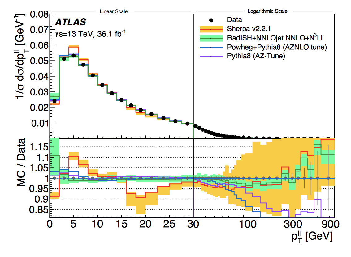
Figure 4: The distribution of the transverse momentum of a lepton pair in Drell-Yan production. The curve labelled with “NNLO+N³LL” includes threshold lograithms resummed to all orders in perturbation theory.

As well as the order of the logs, another potential improvement is to include the terms that we have so far neglected in eq. (16). In particular, whilst a lot is known about the leading power (LP) terms, much less is known about the next-to-leading power (NLP) terms. If the LP terms are dictated by the emission of soft and collinear radiation, the NLP terms are in principle described by next-to-soft (or next-to-collinear) radiation. Coincidentally, this is also a topic that has been widely studied on hep-th in recent years, due in particular to the fact that next-to-soft properties of amplitudes have been linked to symmetries at asymptotic infinity [143, 144, 145], thus starting an ongoing programme known as celestial holography, discussed in chapter 11 of this review [146]. As for the use of Wilson lines discussed above, practitioners in this field may be entirely unaware that the need to understand next-to-soft physics has a highly practical application at the LHC. The need to describe and potentially resum the NLP terms in eq. (16) has been emphasised in e.g. refs. [147, 148, 149, 150, 151]. Indeed, the study of such corrections has a remarkably long history, beginning with the classic work of refs. [152, 153] for massive external particles, which was extended to massless particles in [154]. In QCD, next-to-soft effects have been investigated using a variety of techniques, including diagrammatic approaches [155, 156, 157, 158, 159, 160, 161, 162, 163, 164, 165] that aim to extend the factorisation formula of eq. (18) to NLP order and / or resum NLP logs, insights from fixed-order perturbation theory [166, 167, 168, 169, 170, 171, 172, 173, 174, 175, 176, 177], and effective field theory [178, 179, 180, 181, 182, 183, 184, 185, 186, 187, 188, 189, 190, 191, 192, 193, 194, 195, 196, 197, 198, 199, 200, 201]. We are just starting to learn how to resum NLP effects for certain specific processes, and the coming years are likely to see a rapid increasing of our understanding of their importance. Furthermore, extensions to the factorisation formula of eq. (18) involve new universal objects in field theory, that may be of interest beyond QCD, for those wishing to classify new structures in e.g. ${\cal N}=4$ SYM theory.

We have here seen some basic ideas from threshold resummation, which involves the inclusion of arbitrary amounts of soft / collinear radiation. However, the idea of summing up corrections to all orders in perturbation theory clearly generalises. Another kinematic limit that has been widely studied is the Regge limit, in which the centre of mass energy is much larger than the momentum transfer. This limit becomes experimentally more relevant as the energy of particle accelerators increases, and there is significant evidence that the inclusion of enhanced effects in this limit is needed to better describe scattering data (see e.g. refs. [202, 203, 204, 205, 206, 207, 208, 209, 210, 211, 212]). This makes direct contact with much earlier work on S-matrix theory (see the classic texts of refs. [213, 214], and ref. [215] for a more modern review), ideas from which (e.g. the bootstrap) seem to be coming back into fashion in contemporary hep-th physics. Of course, with any resummation, only a subset of the full information at each order in perturbation theory is included at higher orders. Resummation thus proceeds in tandem with fixed-order perturbation theory to provide a two-pronged attack on QFT: given any observable we want to calculate, we must include as much information as possible. Low-order information in perturbation theory can be calculated exactly, and then supplemented with higher-order results from resummation, being careful that no contributions have been counted twice. There are then two frontiers in perturbation theory, namely the inclusion of subleading terms in both the coupling (NLO, NNLO, …) and logarithmic (NLL, NNLL, …) expansions. Each of these requires clever thinking and new techniques, and also a joined-up approach. For example, new methods for obtaining fixed-order results can often be recycled for calculating higher-order Wilson line correlators, which are needed for resummation. There is significant scope for more formal amplitudists to contribute to both areas.

7 From theory to experiment

In the previous two sections, we have sketched the status of modern-day efforts to calculate perturbative QFT observables for collider physics. Anyone working in this area knows how extraordinarily difficult it can be to squeeze new results out of a non-abelian gauge theory. However, as we already hinted at in section 3, the output of even the most intricate QFT calculation looks almost nothing like what comes out of a particle accelerator! To illustrate this, figure 5 shows an event that was measured by the ATLAS detector in 2016, and which was believed to be a Higgs boson decaying to two Z bosons, which themselves then decay to a pair of leptons each. The upper-left panel shows a cross-sectional slice through the cylindrical detector, where the red and green lines constitute the best guess for what the leptons did. However, there is an enormous number of additional particles. The yellow lines denote extra charged particles that accompanied the Higgs boson event. Many of these will be charged hadrons, which arose from additional quark and gluon radiation. The sheer number of these goes way beyond what we can reliably calculate in fixed-order perturbation theory. What’s more, only a tiny fraction of these charged particles have been kept in the event display - those with sufficiently small momentum transverse to the beam direction are thrown away so that we can even see what is going on! The grey lines demonstrate an additional complication: the beams at the LHC do not consist of single protons, but bunches of many protons (with over 100 billion protons per bunch in fact). This means that a large number of collisions happen simultaneously, so that any event we want to look at is swamped not just by its own mess, but by that of many other independent collisions! This is called pile-up, and can be corrected for by carefully ascertaining that the various particle tracks originate from different scattering vertices, as is shown in the lower panel of the figure. However, it is clear that many theorist’s idea of what “comparing theory to data” means, is very far indeed from what actually happens in practice. Our aim here is to provide a brief review on how QFT can nevertheless be meaningfully applied to the analysis of scattering events, and to point out some of the open issues.

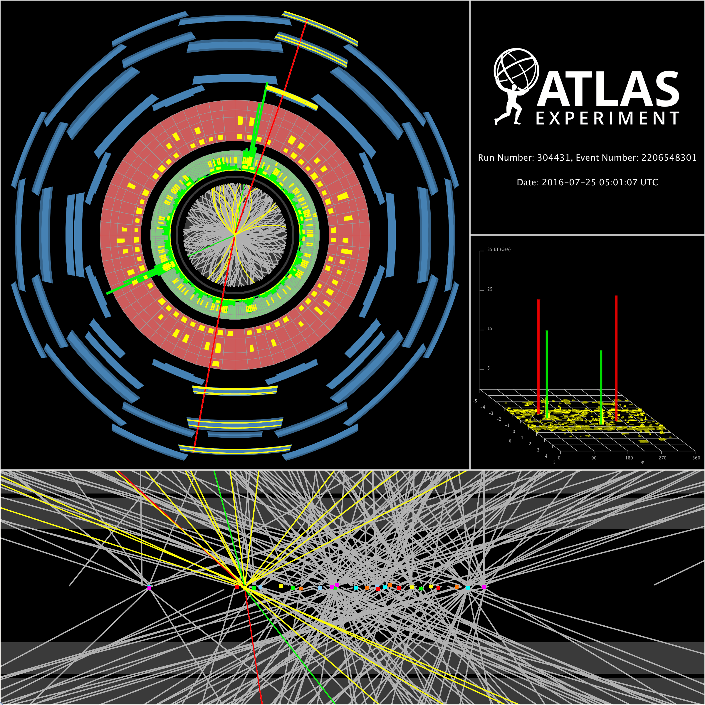
Figure 5: Event display from the ATLAS experiment, for a candidate event in which a Higgs boson decays to two Z bosons. The event was used in the analysis of ref. [216].

Theory calculations have two uses. Either we are calculating a signal (e.g. a new physics process), in which case we want to compare our prediction for a particular observable (e.g. a cross-section) with something measured. Or we might be considering a background, namely a Standard Model process that is in principle different to the signal, but which may contribute a proportion of events that happen to look similar. If the background process is much more probable than the signal, we will get lots of events that mimic the signal and thus act as “fake news”. Experimentalists apply very stringent statistical techniques to make sure that any signal they find has negligible probability of having been caused by a background. However, to do this, they need to know the background processes very very precisely, and this is then the job of theorists. But how do the latter turn their calculations into something approaching what is seen in the collider?

The first problem is to try to estimate the effect of large amounts of additional quark and gluon radiation, and there is a very well-established way to do this known as a parton shower (see e.g. refs. [87, 217] for reviews). It relies on the observation made above, that collinear radiation is enhanced, and also factorises off from an underlying hard scattering process in a universal (process-independent) manner. The radiation is in fact described by known splitting functions which, roughly speaking, give the probability that a parton splits into two other partons, each carrying a certain momentum fraction of the parent. The factorisation property means that different collinear splittings are uncorrelated and independent, and this allows for the construction of an algorithm for the generation of arbitrary amounts of collinear radiation, modelled as a Markov chain process. Essentially, one can generate a set of 4-momenta for the additional particles, whose probability is given by a known distribution, which becomes exact in the limit in which all the radiation is strictly collinear. It includes both real and virtual QFT corrections, so that all probability weights are infrared finite, and applies this distribution even for radiation that is not collinear. That this turns out to be a reasonable approximation follows from the fact that collinear radiation is anyway enhanced. A schematic view of the action of a parton shower is shown in figure 6.

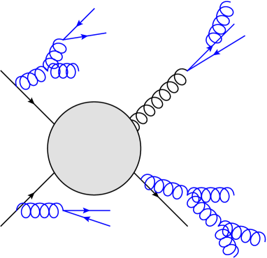
Figure 6: A parton shower algorithm dresses a given hard scattering process (whose particles are shown here in black) with additional quark and gluon radiation (shown in blue). The generated probability for such a process is approximate, but exact in the limit in which the emitted radiation is collinear with the outgoing hard particles. The approximation can be improved by including higher-order information in the hard scattering process.

The energy of modern colliders such as the LHC is such that many particles are produced, which are widely separated in the detector and thus not necessarily collinear. Then the parton shower approximation is insufficient, and must be made more accurate. One way to do this is to include also full higher-order tree-level amplitudes, which can be done up to a few extra legs. One can then invent a suitable matching prescription, that guarantees that the most widely separated particles in any event are described by the tree-level amplitudes (where these are most accurate), but the remaining particles with less separation are described by the parton shower. Several prescriptions exist (see e.g. refs. [218, 219] for some of the first), and they must carefully make sure that no radiation is double-counted, by being included in both the higher-order tree-level matrix elements and the parton shower. From a QFT point of view, including only tree-level amplitudes is not ideal, given that the formal accuracy of the total cross-section then remains at LO only. Thus, it is desirable to start with full NLO amplitudes, and to match these with a parton shower. The matching procedure is now even more delicate than the tree-level case discussed above: the NLO matrix elements contain both real and virtual corrections, both of which potentially overlap with what the parton shower is doing. Two NLO matching schemes are in widespread use [220, 221], and their predictions for a given process are often compared as a means of estimating the reliability of the matching procedure. The state-of-the art for many LHC analyses is that either tree-level amplitudes matched to a parton shower are used, or the NLO approach (which only includes one additional emission in the amplitude). The choice of which approach to use is dictated by what is deemed to be more accurate for the observable of interest. However, one can clearly go further than this, by combining as many NⁿLO matrix elements as possible (including higher-order tree-level matrix elements), and matching the whole lot to a parton shower. The subtleties in doing this are many, and the computational expense of doing this means that more understanding is needed of where such corrections are genuinely important. This is a topic that will evolve a great deal in the coming years [222].

After a parton shower has been applied, our QFT results start to look a lot more like those in figure 5. But they still contain free (anti-)quarks and gluons in the final state, rather than the colour-singlet hadrons that we now are observed in real experiments, due to the confinement property of QCD. For many observables this is not a problem. If all we want to do is to estimate a total cross-section, for example, every parton will end up in some hadron, so the observables calculated assuming final-state partons, or final-state hadrons must be the same. But if we want to more realistically model scattering events for use in experimental analyses, we do indeed want to estimate how the process of hadronisation changes the final state. In practice, this is done using a variety of phenomenological models, containing free parameters that can be tuned to data. What helps is that the quantitative effect of hadronisation on a given observable is known to be suppressed by powers of the QCD confinement scale $\Lambda$ i.e. it constitutes a power correction as appears in eq. (9).

After parton showering and hadronisation, our scattering events are still not fully realistic: we have to include the fact that the incoming partons were only part of the incoming protons. The rest of the latter will somehow be distributed throughout a given scattering event, and their colour information may be non-trivially entangled with the rest of the event. Various models exist for describing this mess, which is loosely referred to as the underlying event. New ideas are always needed, as the uncertainties involved in such models can have dramatic effects. For example, the mass of the top quark is currently measured to within about 0.5 GeV, which is very similar to the estimated theory uncertainty due to underlying event effects (in particular how the colour of the top quark interacts with the colour of the beam remnants). This may not sound like a problem, but the top quark mass enters the expression for quantum corrections to the potential energy of the Higgs field. This can become negative for a certain range of top mass values, which results in the vacuum of our universe becoming unstable. Given the measured Higgs mass value, the mass of the top quark we currently observe is perilously close to the unstable range. We can’t quite say how close, without knowing the top quark mass more precisely, and thus our ability to settle our collective fate rests on better modelling of non-perturbative QCD!

The above steps are computationally technical, and clearly very complicated for the uninitiated. However, various general purpose computer programs exist that allow users to simulate scattering events for a given process, including higher-order amplitudes, parton showers, hadronisation, underlying event modelling, and more besides. They are usually referred to as Monte Carlo event generators, and popular programs include [223, 40, 42, 41]. The output of such programs consists of a set of simulated scattering events, comprising a list of particles (e.g. leptons, photons, hadrons) and their 4-momenta. One may then write additional code for analysing these events, e.g. to select those events that look interesting, and then plot distributions of various measurable quantities, to mimic what is done in an actual collider experiment.

Monte Carlo event generators are widely used both by experimentalists, but also phenomenologists who are trying to find new and better things to measure. They can also be interfaced with further simulations, that mimic the behaviour of the real ATLAS and CMS detectors, for an even more realistic characterisation of how actual scattering events are likely to behave. This then gives various levels at which theorists may compare their results with data, and examples include:

• Parton level: in this case, experimentalists will try to correct for non-perturbative effects, decays of particles etc., and present results for (differential) cross-sections containing final-state partons, vector bosons, top quarks etc. Theorists can then calculate simple final states involving quarks, gluons and other particles, using their favourite methods for calculating scattering amplitudes, for direct comparison with the “data”. This approach is going out of fashion for differential observables, due to the many assumptions that go in to unfolding the raw data back to parton level. If these assumptions turn out to be incorrect or superceded years after an experiment finishes, it can be impossible to replace them with a more correct analysis, especially if the raw data is no longer available.

• Particle / hadron level: Here the theory calculation will include a parton shower, hadronisation, underlying event etc., as is obtained as the output of a Monte Carlo event generator. For some very inclusive observables (e.g. total cross-sections), this is not necessary, given that the additional steps needed to get to particle level will not change the total cross-section. However, the output of a particle-level calculation is a set of simulated scattering events that looks much closer to what happens in a real detector. In particular, this allows theorists to simulate the effect of proposed experimental analyses, including how “interesting” scattering events will be selected, and what the distributions of various measured quantities will look like.

• Detector level: This is similar to particle-level, but includes an additional detector simulation, which would be important for theorists if they believed that realistic detector effects (e.g. finite energy / momentum resolution, gaps in where particles can be recorded) may be affecting their predictions.

For differential cross-sections, particle level has become a standard way of comparing theory with data. Even in that case, however, further steps are usually needed to make experimental events look similar to particle-level predictions. Both experimental scattering events and simulated particle-level ones will contain hundreds of particles, most of which will be hadrons, due to the large amounts of strongly-coupled quark and gluon radiation. In order to simplify each event, we can cluster these particles into jets, using a suitable jet algorithm. We can then select interesting events based on how many jets they have, and what the distribution of these jets looks like in the detector. A surprising amount of care is needed to make sure that a given definition of how to cluster particles into jets is well-defined in perturbation theory (see ref. [224] for an excellent review).

The detailed comparison of theory with data requires a constant dialogue between theorists and experimentalists. At the heart of all event generators that are used in this process lie our beloved scattering amplitudes, and thus new techniques from formal theory can clearly contribute to the ongoing vast international efforts to understand what the universe is trying to tell us in our detectors.

8 Summary

In the previous sections, we have seen a large number of steps in between the calculation of scattering amplitudes, and the direct comparison of theory with quantities measured by experimentalists. It is thus useful to have a quick summary of these ideas, with some further context of how they are applied in practice:

1. Squared amplitudes must be renormalised to remove UV singularities, and converted into cross-sections by integrating over the phase space of any final-state particles, and dividing by the Lorentz-invariant flux factor.

2. At hadron colliders, one must combine cross-sections for incoming partons (i.e. (anti-)quarks and gluons) with parton distribution functions for the incoming beam particles (e.g. protons).

3. Theoretical quantities (e.g. (differential) cross-sections) should be such that they are infrared-safe: final states with different numbers of particles must be combined so that there are no IR singularities in the final results. One should then include as many perturbative orders in each amplitude as possible.

4. If the coefficients of the perturbation expansion are unstable, it may be necessary to include additional logarithmically-enhanced terms to all orders in perturbation theory (“resummation”), and to avoid double-counting contributions which have already been included in the fixed-order expansion.

5. One can approximate the emission of additional QCD radiation by applying a parton shower algorithm to the theoretical prediction for a given final state. Care is needed if combining higher-order amplitudes with the parton shower, to avoid double-counting contributions.

6. After the parton shower, one may include further algorithms that simulate the combination of outgoing partons into colour-singlet hadrons, interactions with the beam remnants etc.

Depending on what data we are comparing to, it is not necessary to include all of these steps. To clarify this, let us consider one of the simplest types of observable that an experiment might measure, namely the cross-section for a given process. Experiments sometimes present a best estimate for the total cross-section, having attempted to reconstruct any intermediate unstable particles, and corrected for the finite detector volume etc. This is perhaps the easiest type of data for a theorist to compare to. If they wish, they can use fixed-order perturbation theory to obtain the total cross-section (including the parton distributions if it is a hadron collider) at some order, and then directly compare this number with the data. The theory result will have some uncertainty estimated by varying the renormalisation and factorisation scales. Likewise, the experimental result will also have an uncertainty, which may be split further into estimated systematic and statistical errors. The first of these is due to possible biases in the measurement, whereas the second measures the limited power of a finite data set. If the theory and data numbers agree within their respective uncertainties, then we would say that the theory matches the data. If not, we can statistically quantify the level of disagreement. This corresponds to the parton level comparison outlined above.

Even for total cross-sections, there are more sophisticated approaches. For example, we may wish to resum contributions from certain kinematic regions, the results of which are typically available in dedicated public codes for given processes. It is routine, for example, to include resummed contributions for various top quark and Higgs boson cross-sections. The effect of including these resummed contributions may be to change the central value of our theory prediction, or modify its uncertainty. However, it is still a single number which we can compare with the measured result. An even more complicated approach would be to dress our theoretical prediction with a parton shower algorithm, hadronisation etc. This simulates final states with large numbers of particles, and we can then apply similar selection criteria to those used in the experiment to our simulated events, in order to reproduce the steps they used in performing their own measurement. This is particularly useful if the experiment presents a measured cross-section that does not correspond to the total cross-section one would calculate in QFT, but has some exclusion criteria already applied (e.g. requirements that the particles be in certain regions of the detector only).

Other common measurements are differential cross-sections involving numbers of particles or jets, or their kinematic properties (e.g. angles, transverse momenta etc.). For low numbers of particles, it may be possible to rely purely on fixed-order perturbation theory, provided there are enough particles in the final state of the relevant amplitudes to coincide with all the particles one wants for a given kinematic distribution. However, a much more realistic estimate will be obtained by using parton-shower programs to simulate realistic events containing many particles, and then clustering the particles into jets using the same algorithms that the experiment has used. In order to do this, a theorist would use one of the publicly available Monte Carlo event generators mentioned above.

Concrete examples of processes at the LHC for which the above remarks apply are perhaps too numerous to list explicitly. Furthermore, modern-day Monte Carlo event generators essentially allow the user to specify any desired process, and then to automatically generate simulated events which can be analysed to produce kinematic distributions for comparison with real data. A particularly convenient repository for experimental data in particle physics is the HEPData database [225], which also provides links to the relevant publications.

Finally, it is worth commenting on what theory input is missing for forthcoming data analyses and / or new collider experiments beyond the currently running LHC. Broadly speaking, the answer is that we must learn to compute ever-higher orders in perturbation theory, and to be able to match amplitudes calculated at these orders to state-of-the-art parton-shower algorithms, where the latter can also be improved. Given the large amount of effort involved, it is necessary to prioritise those processes that experiments are particularly focused on. To this end, wishlists such as those in ref. [68] are highly useful, as they distil the opinions of large numbers of experimentalists into a coherent request! Another area requiring improvement is the determination of the parton distribution functions, as the uncertainty on extracting these from data can limit the theoretical precision of a given collider prediction, if the relevant cross-section is known to a very high perturbative order. It is currently not definitively known what the next collider after the LHC will be. However, it is highly likely to be a lepton-based machine (e.g. colliding electrons and positrons). Many high-precision cross-sections are already known for such colliders, given that the calculations are actually somewhat simpler than those needed for hadron machines, due to the lack of coloured particles in the initial state. But it is always useful to have higher orders in perturbation theory, as for hadron colliders.

9 Conclusion

It is well-known that scattering amplitudes in perturbative QFT are relevant for collider experiments. But the precise way in which they are used, including the huge number of steps that are needed to meaningfully compare theory with data, are never dealt with in textbooks. It is perfectly possible nowadays for formal theorists to live out an entire career without comparing anything to data, despite a desire to do so. It is also very often true that the topics being discussed on hep-th (e.g. Wilson lines, (next-to)-soft radiation) are the same topics being discussed on hep-ph, albeit in completely different notation, and for entirely different reasons. Hence, there is significant scope for more formal theorists to contribute to the challenging and rewarding world of collider physics, should they wish to do so. Recent years have seen remarkable revolutions in how we think about scattering amplitudes in different theories, and how those different theories are related. My hope – which is also the very ethos of the SAGEX network – is that the coming years will see similar revolutions in how we apply new techniques to extract the most we can from current and forthcoming collider experiments.

References

- [1] Aaboud M et al. (ATLAS) 2020 Eur. Phys. J. C 80 754 (Preprint 1903.07570)
- [2] Anastasiou C, Duhr C, Dulat F, Herzog F and Mistlberger B 2015 Phys. Rev. Lett. 114 212001 (Preprint 1503.06056)
- [3] Anastasiou C, Duhr C, Dulat F, Furlan E, Gehrmann T, Herzog F, Lazopoulos A and Mistlberger B 2016 JHEP 05 058 (Preprint 1602.00695)
- [4] Dreyer F A and Karlberg A 2016 Phys. Rev. Lett. 117 072001 (Preprint 1606.00840)
- [5] Dreyer F A and Karlberg A 2018 Phys. Rev. D 98 114016 (Preprint 1811.07906)
- [6] Duhr C, Dulat F and Mistlberger B 2020 Phys. Rev. Lett. 125 172001 (Preprint 2001.07717)
- [7] Gross D J and Wilczek F 1973 Phys. Rev. Lett. 30 1343--1346
- [8] Politzer H D 1973 Phys. Rev. Lett. 30 1346--1349
- [9] Feynman R P 1969 Conf. Proc. C 690905 237--258
- [10] Feynman R P 1969 Phys. Rev. Lett. 23 1415--1417
- [11] Collins J C 1986 Renormalization: An Introduction to Renormalization, The Renormalization Group, and the Operator Product Expansion (Cambridge Monographs on Mathematical Physics vol 26) (Cambridge: Cambridge University Press) ISBN 978-0-521-31177-9, 978-0-511-86739-2
- [12] Bloch F and Nordsieck A 1937 Phys. Rev. 52 54--59
- [13] Kinoshita T 1962 J. Math. Phys. 3 650--677
- [14] Lee T D and Nauenberg M 1964 Phys. Rev. 133 B1549--B1562
- [15] Bailey S, Cridge T, Harland-Lang L A, Martin A D and Thorne R S 2021 Eur. Phys. J. C 81 341 (Preprint 2012.04684)
- [16] Abdul Khalek R et al. (NNPDF) 2019 Eur. Phys. J. C 79 931 (Preprint 1906.10698)
- [17] Alekhin S, Blümlein J and Moch S 2018 Eur. Phys. J. C 78 477 (Preprint 1803.07537)
- [18] Hou T J et al. 2021 Phys. Rev. D 103 014013 (Preprint 1912.10053)
- [19] Passarino G and Veltman M J G 1979 Nucl. Phys. B 160 151--207
- [20] Ellis R K and Zanderighi G 2008 JHEP 02 002 (Preprint 0712.1851)
- [21] Bern Z, Dixon L J, Dunbar D C and Kosower D A 1994 Nucl. Phys. B 425 217--260 (Preprint hep-ph/9403226)
- [22] Bern Z, Dixon L J, Dunbar D C and Kosower D A 1995 Nucl. Phys. B 435 59--101 (Preprint hep-ph/9409265)
- [23] Bern Z and Morgan A G 1996 Nucl. Phys. B 467 479--509 (Preprint hep-ph/9511336)
- [24] Bern Z, Dixon L J and Kosower D A 1998 Nucl. Phys. B 513 3--86 (Preprint hep-ph/9708239)
- [25] Britto R, Cachazo F and Feng B 2005 Nucl. Phys. B 725 275--305 (Preprint hep-th/0412103)
- [26] Brandhuber A, McNamara S, Spence B J and Travaglini G 2005 JHEP 10 011 (Preprint hep-th/0506068)
- [27] Britto R, Cachazo F and Feng B 2005 Nucl. Phys. B 715 499--522 (Preprint hep-th/0412308)
- [28] Bern Z, Dixon L J and Kosower D A 2005 Phys. Rev. D 71 105013 (Preprint hep-th/0501240)
- [29] Bern Z, Dixon L J and Kosower D A 2005 Phys. Rev. D 72 125003 (Preprint hep-ph/0505055)
- [30] Badger S D, Glover E W N, Khoze V V and Svrcek P 2005 JHEP 07 025 (Preprint hep-th/0504159)
- [31] Badger S D, Glover E W N and Khoze V V 2006 JHEP 01 066 (Preprint hep-th/0507161)
- [32] Anastasiou C, Britto R, Feng B, Kunszt Z and Mastrolia P 2007 Phys. Lett. B 645 213--216 (Preprint hep-ph/0609191)
- [33] Anastasiou C, Britto R, Feng B, Kunszt Z and Mastrolia P 2007 JHEP 03 111 (Preprint hep-ph/0612277)
- [34] Giele W T, Kunszt Z and Melnikov K 2008 JHEP 04 049 (Preprint 0801.2237)
- [35] Huang Y t and McGady D 2014 Phys. Rev. Lett. 112 241601 (Preprint 1307.4065)
- [36] Ellis R K, Kunszt Z, Melnikov K and Zanderighi G 2012 Phys. Rept. 518 141--250 (Preprint 1105.4319)
- [37] Gleisberg T and Krauss F 2008 Eur. Phys. J. C 53 501--523 (Preprint 0709.2881)
- [38] Hirschi V, Frederix R, Frixione S, Garzelli M V, Maltoni F and Pittau R 2011 JHEP 05 044 (Preprint 1103.0621)
- [39] Bellm J et al. 2016 Eur. Phys. J. C 76 196 (Preprint 1512.01178)
- [40] Bothmann E et al. (Sherpa) 2019 SciPost Phys. 7 034 (Preprint 1905.09127)
- [41] Alwall J, Frederix R, Frixione S, Hirschi V, Maltoni F, Mattelaer O, Shao H S, Stelzer T, Torrielli P and Zaro M 2014 JHEP 07 079 (Preprint 1405.0301)
- [42] Bellm J et al. 2020 Eur. Phys. J. C 80 452 (Preprint 1912.06509)
- [43] Abreu S, Britto R and Duhr C 2022 J. Phys. A 55 443004 (Preprint 2203.13014)
- [44] Blümlein J and Schneider C 2022 J. Phys. A 55 443005 (Preprint 2203.13015)
- [45] Papathanasiou G 2022 J. Phys. A 55 443006 (Preprint 2203.13016)
- [46] Travaglini G et al. 2022 J. Phys. A 55 443001 (Preprint 2203.13011)
- [47] Frixione S, Kunszt Z and Signer A 1996 Nucl. Phys. B 467 399--442 (Preprint hep-ph/9512328)
- [48] Catani S and Seymour M H 1997 Nucl. Phys. B 485 291--419 [Erratum: Nucl.Phys.B 510, 503--504 (1998)] (Preprint hep-ph/9605323)
- [49] Gehrmann-De Ridder A, Gehrmann T and Glover E W N 2005 JHEP 09 056 (Preprint hep-ph/0505111)
- [50] Currie J, Glover E W N and Wells S 2013 JHEP 04 066 (Preprint 1301.4693)
- [51] Czakon M 2010 Phys. Lett. B 693 259--268 (Preprint 1005.0274)
- [52] Czakon M 2011 Nucl. Phys. B 849 250--295 (Preprint 1101.0642)
- [53] Boughezal R, Melnikov K and Petriello F 2012 Phys. Rev. D 85 034025 (Preprint 1111.7041)
- [54] Anastasiou C, Melnikov K and Petriello F 2004 Phys. Rev. D 69 076010 (Preprint hep-ph/0311311)
- [55] Binoth T and Heinrich G 2004 Nucl. Phys. B 693 134--148 (Preprint hep-ph/0402265)
- [56] Catani S and Grazzini M 2007 Phys. Rev. Lett. 98 222002 (Preprint hep-ph/0703012)
- [57] Boughezal R, Liu X and Petriello F 2015 Phys. Rev. D 91 094035 (Preprint 1504.02540)
- [58] Gaunt J, Stahlhofen M, Tackmann F J and Walsh J R 2015 JHEP 09 058 (Preprint 1505.04794)
- [59] Del Duca V, Duhr C, Somogyi G, Tramontano F and Trócsányi Z 2015 JHEP 04 036 (Preprint 1501.07226)
- [60] Caola F, Melnikov K and Röntsch R 2017 Eur. Phys. J. C 77 248 (Preprint 1702.01352)
- [61] Delto M and Melnikov K 2019 JHEP 05 148 (Preprint 1901.05213)
- [62] Caola F, Melnikov K and Röntsch R 2019 Eur. Phys. J. C 79 386 (Preprint 1902.02081)
- [63] Magnea L, Maina E, Pelliccioli G, Signorile-Signorile C, Torrielli P and Uccirati S 2018 JHEP 12 107 [Erratum: JHEP 06, 013 (2019)] (Preprint 1806.09570)
- [64] Magnea L, Maina E, Pelliccioli G, Signorile-Signorile C, Torrielli P and Uccirati S 2018 JHEP 12 062 (Preprint 1809.05444)
- [65] Caola F, Melnikov K and Röntsch R 2019 Eur. Phys. J. C 79 1013 (Preprint 1907.05398)
- [66] Asteriadis K, Caola F, Melnikov K and Röntsch R 2020 Eur. Phys. J. C 80 8 (Preprint 1910.13761)
- [67] Cacciari M, Dreyer F A, Karlberg A, Salam G P and Zanderighi G 2015 Phys. Rev. Lett. 115 082002 [Erratum: Phys.Rev.Lett. 120, 139901 (2018)] (Preprint 1506.02660)
- [68] Huss A, Huston J, Jones S and Pellen M 2022 (Preprint 2207.02122)
- [69] Denner A and Dittmaier S 2020 Phys. Rept. 864 1--163 (Preprint 1912.06823)
- [70] Agarwal N, Magnea L, Signorile-Signorile C and Tripathi A 2021 (Preprint 2112.07099)
- [71] Parisi G 1980 Phys. Lett. B 90 295--296
- [72] Curci G and Greco M 1980 Phys. Lett. B 92 175--178
- [73] Sterman G F 1987 Nucl. Phys. B 281 310--364
- [74] Catani S and Trentadue L 1989 Nucl. Phys. B 327 323--352
- [75] Gatheral J G M 1983 Phys. Lett. B 133 90--94
- [76] Frenkel J and Taylor J C 1984 Nucl. Phys. B 246 231--245
- [77] Sterman G F 1981 AIP Conf. Proc. 74 22--40
- [78] Korchemsky G P and Marchesini G 1993 Nucl. Phys. B 406 225--258 (Preprint hep-ph/9210281)
- [79] Korchemsky G P and Marchesini G 1993 Phys. Lett. B 313 433--440
- [80] Forte S and Ridolfi G 2003 Nucl. Phys. B 650 229--270 (Preprint hep-ph/0209154)
- [81] Becher T and Neubert M 2006 Phys. Rev. Lett. 97 082001 (Preprint hep-ph/0605050)
- [82] Schwartz M D 2008 Phys. Rev. D 77 014026 (Preprint 0709.2709)
- [83] Bauer C W, Fleming S P, Lee C and Sterman G F 2008 Phys. Rev. D 78 034027 (Preprint 0801.4569)
- [84] Chiu J y, Fuhrer A, Kelley R and Manohar A V 2009 Phys. Rev. D 80 094013 (Preprint 0909.0012)
- [85] Luisoni G and Marzani S 2015 J. Phys. G 42 103101 (Preprint 1505.04084)
- [86] Becher T, Broggio A and Ferroglia A 2015 Introduction to Soft-Collinear Effective Theory vol 896 (Springer) (Preprint 1410.1892)
- [87] Campbell J, Huston J and Krauss F 2017 The Black Book of Quantum Chromodynamics: A Primer for the LHC Era (Oxford University Press) ISBN 978-0-19-965274-7
- [88] Dixon L J, Magnea L and Sterman G F 2008 JHEP 08 022 (Preprint 0805.3515)
- [89] Weinberg S 1965 Phys. Rev. 140 B516--B524
- [90] Alday L F and Maldacena J M 2007 JHEP 06 064 (Preprint 0705.0303)
- [91] Polyakov A M 1980 Nucl. Phys. B 164 171--188
- [92] Arefeva I Y 1980 Phys. Lett. B 93 347--353
- [93] Dotsenko V S and Vergeles S N 1980 Nucl. Phys. B 169 527--546
- [94] Brandt R A, Neri F and Sato M a 1981 Phys. Rev. D 24 879
- [95] Korchemsky G P and Radyushkin A V 1986 Phys. Lett. B 171 459--467
- [96] Korchemsky G P and Radyushkin A V 1986 Sov. J. Nucl. Phys. 44 877
- [97] Korchemsky G P and Radyushkin A V 1987 Nucl. Phys. B 283 342--364
- [98] Grozin A, Henn J M, Korchemsky G P and Marquard P 2016 JHEP 01 140 (Preprint 1510.07803)
- [99] Grozin A, Henn J M, Korchemsky G P and Marquard P 2015 Phys. Rev. Lett. 114 062006 (Preprint 1409.0023)
- [100] Brüser R, Dlapa C, Henn J M and Yan K 2021 Phys. Rev. Lett. 126 021601 (Preprint 2007.04851)
- [101] Korchemsky G P 1994 Phys. Lett. B 325 459--466 (Preprint hep-ph/9311294)
- [102] Korchemskaya I A and Korchemsky G P 1996 Phys. Lett. B 387 346--354 (Preprint hep-ph/9607229)
- [103] Korchemskaya I A and Korchemsky G P 1995 Nucl. Phys. B 437 127--162 (Preprint hep-ph/9409446)
- [104] Catani S 1998 Phys. Lett. B 427 161--171 (Preprint hep-ph/9802439)
- [105] Sterman G F and Tejeda-Yeomans M E 2003 Phys. Lett. B 552 48--56 (Preprint hep-ph/0210130)
- [106] Kidonakis N, Oderda G and Sterman G F 1998 Nucl. Phys. B 531 365--402 (Preprint hep-ph/9803241)
- [107] Bonciani R, Catani S, Mangano M L and Nason P 2003 Phys. Lett. B 575 268--278 (Preprint hep-ph/0307035)
- [108] Dokshitzer Y L and Marchesini G 2006 JHEP 01 007 (Preprint hep-ph/0509078)
- [109] Aybat S M, Dixon L J and Sterman G F 2006 Phys. Rev. D 74 074004 (Preprint hep-ph/0607309)
- [110] Gardi E and Magnea L 2009 JHEP 03 079 (Preprint 0901.1091)
- [111] Becher T and Neubert M 2009 Phys. Rev. Lett. 102 162001 [Erratum: Phys.Rev.Lett. 111, 199905 (2013)] (Preprint 0901.0722)
- [112] Becher T and Neubert M 2009 JHEP 06 081 [Erratum: JHEP 11, 024 (2013)] (Preprint 0903.1126)
- [113] Gardi E and Magnea L 2009 Nuovo Cim. C 32N5-6 137--157 (Preprint 0908.3273)
- [114] Dixon L J 2009 Phys. Rev. D 79 091501 (Preprint 0901.3414)
- [115] Dixon L J, Gardi E and Magnea L 2010 JHEP 02 081 (Preprint 0910.3653)
- [116] Del Duca V, Duhr C, Gardi E, Magnea L and White C D 2011 JHEP 12 021 (Preprint 1109.3581)
- [117] Caron-Huot S 2015 JHEP 05 093 (Preprint 1309.6521)
- [118] Ahrens V, Neubert M and Vernazza L 2012 JHEP 09 138 (Preprint 1208.4847)
- [119] Naculich S G, Nastase H and Schnitzer H J 2013 JHEP 04 114 (Preprint 1301.2234)
- [120] Erdoğan O and Sterman G 2015 Phys. Rev. D 91 065033 (Preprint 1411.4588)
- [121] Gehrmann T, Glover E W N, Huber T, Ikizlerli N and Studerus C 2010 JHEP 06 094 (Preprint 1004.3653)
- [122] Agarwal B, von Manteuffel A, Panzer E and Schabinger R M 2021 Phys. Lett. B 820 136503 (Preprint 2102.09725)
- [123] Almelid O, Duhr C and Gardi E 2016 Phys. Rev. Lett. 117 172002 (Preprint 1507.00047)
- [124] Gardi E, Almelid O and Duhr C 2016 PoS LL2016 058 (Preprint 1606.05697)
- [125] Kidonakis N 2009 Phys. Rev. Lett. 102 232003 (Preprint 0903.2561)
- [126] Mitov A, Sterman G F and Sung I 2009 Phys. Rev. D 79 094015 (Preprint 0903.3241)
- [127] Becher T and Neubert M 2009 Phys. Rev. D 79 125004 [Erratum: Phys.Rev.D 80, 109901 (2009)] (Preprint 0904.1021)
- [128] Beneke M, Falgari P and Schwinn C 2010 Nucl. Phys. B 828 69--101 (Preprint 0907.1443)
- [129] Czakon M, Mitov A and Sterman G F 2009 Phys. Rev. D 80 074017 (Preprint 0907.1790)
- [130] Ferroglia A, Neubert M, Pecjak B D and Yang L L 2009 JHEP 11 062 (Preprint 0908.3676)
- [131] Mitov A, Sterman G F and Sung I 2010 Phys. Rev. D 82 034020 (Preprint 1005.4646)
- [132] Gardi E 2014 JHEP 04 044 (Preprint 1310.5268)
- [133] Falcioni G, Gardi E, Harley M, Magnea L and White C D 2014 JHEP 10 010 (Preprint 1407.3477)
- [134] Henn J M, Smirnov A V and Smirnov V A 2013 JHEP 07 128 (Preprint 1306.2799)
- [135] Gardi E, Laenen E, Stavenga G and White C D 2010 JHEP 11 155 (Preprint 1008.0098)
- [136] Gardi E and White C D 2011 JHEP 03 079 (Preprint 1102.0756)
- [137] Dukes M, Gardi E, Steingrimsson E and White C D 2013 J. Comb. Theor. A 120 1012--1037 (Preprint 1301.6576)
- [138] Gardi E, Smillie J M and White C D 2013 JHEP 06 088 (Preprint 1304.7040)
- [139] Gardi E, Harley M, Lodin R, Palusa M, Smillie J M, White C D and Yeomans S 2021 (Preprint 2110.01685)
- [140] Mitov A, Sterman G and Sung I 2010 Phys. Rev. D 82 096010 (Preprint 1008.0099)
- [141] Vladimirov A A 2015 JHEP 06 120 (Preprint 1501.03316)
- [142] Almelid O, Duhr C, Gardi E, McLeod A and White C D 2017 JHEP 09 073 (Preprint 1706.10162)
- [143] Cachazo F and Strominger A 2014 (Preprint 1404.4091)
- [144] Casali E 2014 JHEP 08 077 (Preprint 1404.5551)
- [145] Strominger A 2017 (Preprint 1703.05448)
- [146] McLoughlin T, Puhm A and Raclariu A M 2022 J. Phys. A 55 443012 (Preprint 2203.13022)
- [147] Kramer M, Laenen E and Spira M 1998 Nucl. Phys. B 511 523--549 (Preprint hep-ph/9611272)
- [148] Ball R D, Bonvini M, Forte S, Marzani S and Ridolfi G 2013 Nucl. Phys. B 874 746--772 (Preprint 1303.3590)
- [149] Bonvini M, Forte S, Ridolfi G and Rottoli L 2015 JHEP 01 046 (Preprint 1409.0864)
- [150] van Beekveld M, Beenakker W, Basu R, Laenen E, Misra A and Motylinski P 2019 Phys. Rev. D 100 056009 (Preprint 1905.11771)
- [151] van Beekveld M, Laenen E, Sinninghe Damsté J and Vernazza L 2021 JHEP 05 114 (Preprint 2101.07270)
- [152] Low F E 1958 Phys. Rev. 110 974--977
- [153] Burnett T H and Kroll N M 1968 Phys. Rev. Lett. 20 86
- [154] Del Duca V 1990 Nucl. Phys. B 345 369--388
- [155] Laenen E, Stavenga G and White C D 2009 JHEP 03 054 (Preprint 0811.2067)
- [156] Laenen E, Magnea L, Stavenga G and White C D 2011 JHEP 01 141 (Preprint 1010.1860)
- [157] Bonocore D, Laenen E, Magnea L, Melville S, Vernazza L and White C D 2015 JHEP 06 008 (Preprint 1503.05156)
- [158] Bonocore D, Laenen E, Magnea L, Vernazza L and White C D 2016 JHEP 12 121 (Preprint 1610.06842)
- [159] Bonocore D 2021 JHEP 02 007 (Preprint 2009.07863)
- [160] Gervais H 2017 Phys. Rev. D 95 125009 (Preprint 1704.00806)
- [161] Gervais H 2017 Phys. Rev. D 96 065007 (Preprint 1706.03453)
- [162] Gervais H 2017 Soft Radiation Theorems at All Loop Order in Quantum Field Theory Ph.D. thesis
- [163] Laenen E, Sinninghe Damsté J, Vernazza L, Waalewijn W and Zoppi L 2021 Phys. Rev. D 103 034022 (Preprint 2008.01736)
- [164] Bahjat-Abbas N, Bonocore D, Sinninghe Damsté J, Laenen E, Magnea L, Vernazza L and White C D 2019 JHEP 11 002 (Preprint 1905.13710)
- [165] van Beekveld M, Vernazza L and White C D 2021 (Preprint 2109.09752)
- [166] Soar G, Moch S, Vermaseren J A M and Vogt A 2010 Nucl. Phys. B 832 152--227 (Preprint 0912.0369)
- [167] Moch S and Vogt A 2009 JHEP 11 099 (Preprint 0909.2124)
- [168] Moch S and Vogt A 2009 JHEP 04 081 (Preprint 0902.2342)
- [169] de Florian D, Mazzitelli J, Moch S and Vogt A 2014 JHEP 10 176 (Preprint 1408.6277)
- [170] Lo Presti N A, Almasy A A and Vogt A 2014 Phys. Lett. B 737 120--123 (Preprint 1407.1553)
- [171] Del Duca V, Laenen E, Magnea L, Vernazza L and White C D 2017 JHEP 11 057 (Preprint 1706.04018)
- [172] van Beekveld M, Beenakker W, Laenen E and White C D 2020 JHEP 03 106 (Preprint 1905.08741)
- [173] Bonocore D, Laenen E, Magnea L, Vernazza L and White C D 2015 Phys. Lett. B 742 375--382 (Preprint 1410.6406)
- [174] Bahjat-Abbas N, Sinninghe Damsté J, Vernazza L and White C D 2018 JHEP 10 144 (Preprint 1807.09246)
- [175] Ebert M A, Moult I, Stewart I W, Tackmann F J, Vita G and Zhu H X 2018 JHEP 12 084 (Preprint 1807.10764)
- [176] Boughezal R, Isgrò A and Petriello F 2018 Phys. Rev. D 97 076006 (Preprint 1802.00456)
- [177] Boughezal R, Isgrò A and Petriello F 2020 Phys. Rev. D 101 016005 (Preprint 1907.12213)
- [178] Kolodrubetz D W, Moult I and Stewart I W 2016 JHEP 05 139 (Preprint 1601.02607)
- [179] Moult I, Rothen L, Stewart I W, Tackmann F J and Zhu H X 2017 Phys. Rev. D 95 074023 (Preprint 1612.00450)
- [180] Feige I, Kolodrubetz D W, Moult I and Stewart I W 2017 JHEP 11 142 (Preprint 1703.03411)
- [181] Beneke M, Garny M, Szafron R and Wang J 2018 JHEP 03 001 (Preprint 1712.04416)
- [182] Beneke M, Garny M, Szafron R and Wang J 2018 JHEP 11 112 (Preprint 1808.04742)
- [183] Bhattacharya A, Moult I, Stewart I W and Vita G 2019 JHEP 05 192 (Preprint 1812.06950)
- [184] Beneke M, Garny M, Szafron R and Wang J 2019 JHEP 09 101 (Preprint 1907.05463)
- [185] Bodwin G T, Ee J H, Lee J and Wang X P 2021 (Preprint 2107.07941)
- [186] Moult I, Stewart I W and Vita G 2019 JHEP 11 153 (Preprint 1905.07411)
- [187] Beneke M, Broggio A, Jaskiewicz S and Vernazza L 2020 JHEP 07 078 (Preprint 1912.01585)
- [188] Liu Z L and Neubert M 2020 JHEP 04 033 (Preprint 1912.08818)
- [189] Liu Z L, Mecaj B, Neubert M and Wang X 2021 Phys. Rev. D 104 014004 (Preprint 2009.04456)
- [190] Boughezal R, Liu X and Petriello F 2017 JHEP 03 160 (Preprint 1612.02911)
- [191] Moult I, Stewart I W and Vita G 2017 JHEP 07 067 (Preprint 1703.03408)
- [192] Chang C H, Stewart I W and Vita G 2018 JHEP 04 041 (Preprint 1712.04343)
- [193] Moult I, Stewart I W, Vita G and Zhu H X 2018 JHEP 08 013 (Preprint 1804.04665)
- [194] Beneke M, Broggio A, Garny M, Jaskiewicz S, Szafron R, Vernazza L and Wang J 2019 JHEP 03 043 (Preprint 1809.10631)
- [195] Ebert M A, Moult I, Stewart I W, Tackmann F J, Vita G and Zhu H X 2019 JHEP 04 123 (Preprint 1812.08189)
- [196] Beneke M, Garny M, Jaskiewicz S, Szafron R, Vernazza L and Wang J 2020 JHEP 01 094 (Preprint 1910.12685)
- [197] Moult I, Stewart I W, Vita G and Zhu H X 2020 JHEP 05 089 (Preprint 1910.14038)
- [198] Liu Z L and Neubert M 2020 JHEP 06 060 (Preprint 2003.03393)
- [199] Liu Z L, Mecaj B, Neubert M, Wang X and Fleming S 2020 JHEP 07 104 (Preprint 2005.03013)
- [200] Wang J 2019 (Preprint 1912.09920)
- [201] Beneke M, Garny M, Jaskiewicz S, Szafron R, Vernazza L and Wang J 2020 JHEP 10 196 (Preprint 2008.04943)
- [202] White C D and Thorne R S 2007 Phys. Rev. D 75 034005 (Preprint hep-ph/0611204)
- [203] Ball R D, Bertone V, Bonvini M, Marzani S, Rojo J and Rottoli L 2018 Eur. Phys. J. C 78 321 (Preprint 1710.05935)
- [204] Andersen J R, Black J A, Brooks H M, Byrne E P, Maier A and Smillie J M 2021 JHEP 04 105 (Preprint 2012.10310)
- [205] Andersen J R, Hapola T, Heil M, Maier A and Smillie J 2019 (Preprint 1902.08430)
- [206] Andersen J R, Cockburn J D, Heil M, Maier A and Smillie J M 2019 JHEP 04 127 (Preprint 1812.08072)
- [207] Andersen J R, Hapola T, Heil M, Maier A and Smillie J M 2018 JHEP 08 090 (Preprint 1805.04446)
- [208] Andersen J R, Hapola T, Maier A and Smillie J M 2017 JHEP 09 065 (Preprint 1706.01002)
- [209] Andersen J R, Medley J J and Smillie J M 2016 JHEP 05 136 (Preprint 1603.05460)
- [210] Andersen J R, Hapola T and Smillie J M 2012 JHEP 09 047 (Preprint 1206.6763)
- [211] Andersen J R and Smillie J M 2011 JHEP 06 010 (Preprint 1101.5394)
- [212] Andersen J R and Smillie J M 2010 JHEP 01 039 (Preprint 0908.2786)
- [213] Eden R J, Landshoff P V, Olive D I and Polkinghorne J C 1966 The analytic S-matrix (Cambridge: Cambridge Univ. Press)
- [214] Collins P D B 2009 An Introduction to Regge Theory and High-Energy Physics Cambridge Monographs on Mathematical Physics (Cambridge, UK: Cambridge Univ. Press) ISBN 978-0-521-11035-8
- [215] White C D 2020 SciPost Phys. Lect. Notes 13 1 (Preprint 1909.05177)
- [216] Aaboud M et al. (ATLAS) 2017 JHEP 10 132 (Preprint 1708.02810)
- [217] Ellis R K, Stirling W J and Webber B R 2011 QCD and collider physics vol 8 (Cambridge University Press) ISBN 978-0-511-82328-2, 978-0-521-54589-1
- [218] Caravaglios F, Mangano M L, Moretti M and Pittau R 1999 Nucl. Phys. B 539 215--232 (Preprint hep-ph/9807570)
- [219] Catani S, Krauss F, Kuhn R and Webber B R 2001 JHEP 11 063 (Preprint hep-ph/0109231)
- [220] Frixione S and Webber B R 2002 JHEP 06 029 (Preprint hep-ph/0204244)
- [221] Frixione S, Nason P and Webber B R 2003 JHEP 08 007 (Preprint hep-ph/0305252)
- [222] Re E 2021 Recent progress on high order calculations and matching to parton showers 9th Large Hadron Collider Physics Conference (Preprint 2110.02183)
- [223] Sjöstrand T 2020 Comput. Phys. Commun. 246 106910 (Preprint 1907.09874)
- [224] Salam G P 2010 Eur. Phys. J. C 67 637--686 (Preprint 0906.1833)
- [225] HEPData: Repository for publication-related high-energy physics data https://www.hepdata.net accessed: 2022-06-27