Transformer Compressed Sensing via Global Image Tokens

Abstract

Convolutional neural networks (CNN) have demonstrated outstanding Compressed Sensing (CS) performance compared to traditional, hand-crafted methods. However, they are broadly limited in terms of generalisability, inductive bias and difficulty to model long distance relationships. Transformer neural networks (TNN) overcome such issues by implementing an attention mechanism designed to capture dependencies between inputs. However, high-resolution tasks typically require vision Transformers (ViT) to decompose an image into patch-based tokens, limiting inputs to inherently local contexts. We propose a novel image decomposition that naturally embeds images into low-resolution inputs. These Kaleidoscope tokens (KD) provide a mechanism for global attention, at the same computational cost as a patch-based approach. To showcase this development, we replace CNN components in a well-known CS-MRI neural network with TNN blocks and demonstrate the improvements afforded by KD. We also propose an ensemble of image tokens, which enhance overall image quality and reduces model size. Supplementary material is available: https://github.com/uqmarlonbran/TCS.git.

Index Terms—  Kaleidoscope, TNN, ViT, CS, MRI

0.84(0.08,0.93) ©2022 IEEE. Personal use of this material is permitted. Permission from IEEE must be obtained for all other uses, in any current or future media, including reprinting/republishing this material for advertising or promotional purposes, creating new collective works, for resale or redistribution to servers or lists, or reuse of any copyrighted component of this work in other works.

1 Introduction

Transformer neural networks (TNN) have been established as the gold-standard for sequence-to-sequence prediction problems, such as natural language processing [1]. This has been largely attributed to their ability of dynamically adjusting receptive fields, model global dependencies and scale with large amounts of data. The Vision Transformer (ViT) succeeded TNN contributions by delivering state-of-the-art computer vision (CV) performance [2]. ViT improved upon convolutional neural network (CNN)-based image classification and demonstrated superior scaling with model and dataset size. A current topic of research regarding ViT lies in the choice and treatment of the image tokens used as inputs, where naively, patch tokens were initially deployed. Recent work has shown that more efficient image representations can reduce training requirements and overall model size [3, 4, 5, 6, 7].

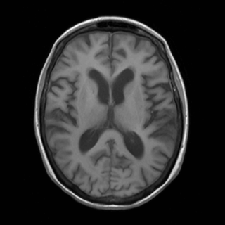
(a) $320\times 320$ sample T1-w brain MRI.

(b) $64\times 64$ Kaleidoscope Embeddings.

Fig. 1: $(\nu=5,\sigma=1)$-KT for token embedding: (a) Input Image; (b) Downsampled and concatenated versions of (a).

More specifically, image patches alone present a high level of difficulty for capturing global structures such as edges and lines [3], and restrict the ViT to a single scale of vision [3, 4]. What followed was a paradigm of hierarchical ViT architectures that aggregate and combine patches in a manner that reduces overall spatial resolution and token size [3, 4, 5]. The objective being to induce an architectural prior that enforces earlier layers to operate on high spatial resolutions, and limit deeper layers to spatially coarse, complex features. While such approaches are useful if dimensionality reduction is desired, it may not be ideal if the output dimension is the same as that of the input. As an alternative to patches, axial tokens have shown great promise for CV tasks [6], wherein attention between rows and columns are evaluated independently. Axial attention can be considered a natural extension of TNN to two-dimensional (2D) data, akin to decomposing the discrete Fourier transform (DFT) of a 2D image into a series of one-dimensional (1D) DFT operations. Axial encoders are primarily handicapped by necessitating two attention blocks per-encoder, double the feed-forward layers, and a bias towards frequency content along the axes. Lastly, it has been discovered that the inherent local bias’ of CNN can help improve training stability and overall CV performance [7]. The central premise being that CNNs are able to perform efficient feature extraction, allowing ViT to make decisions based on these curated inputs.

These advancements within CV have led to active development of ViTs for medical imaging tasks, particularly medical image segmentation [8]. However, despite the advantages compared to CNN equivalents, they have not yet received significant attention for Compressed Sensing (CS). To that end, we propose a ViT-based CS network for CS- magnetic resonance imaging (MRI), which to our knowledge, provides the first convolution-free deep neural network (DNN) that achieves state-of-the-art reconstruction performance. This paper develops the following:

1. Novel Kaleidoscope tokens (KD) that present global image contexts with low-frequency features; improves overall performance compared to patch alternative.

2. A cascaded ViT architecture that separately attends to image features by employing an ensemble of token embeddings.

3. Efficient multi-scale ViT perception without reducing input or image resolution.

The proposed network architecture extends the Deep cascade of Convolutional Neural Networks (DcCNN) [9], wherein CNN components are replaced with TNN encoder layers. This paper experiments with patch, axial, and our novel KD embeddings (see Fig. 1). We demonstrate that a KD-based ViT provides an inherently global context of an image, which when cascaded with patch and axial ViT ensures both global and local features are processed independently. This ensemble of ViT is an efficient method of achieving multi-scale perception, as the separate features are attended to without affecting resolution and the Kaleidoscope transform (KT) [10] needs only the computation cost of “patchifying” an image.

2 Method

2.1 Kaleidoscope Embedding for Image Tokens

The KT was recently proposed by White et al. [10] to explain the fractal nature of Chaotic Sensing in DFT space [11] and formalises the concept of down-sampling and concatenating an image with itself. For example, a $\nu,\sigma$-KT decomposes an image into $\nu^{2}$ down-sampled copies where each is scaled by a factor of $\sigma$. In this work, we efficiently achieve an arbitrary down-sampling factor $\nu$, and smear factor $\sigma=1$, via element reordering. As seen in Fig. 1 for a $(5,1)$-KT, $25$ pixel-shifted low-resolution copies of the original image are produced. Image tokens arise via linear projection of the flattened low-resolution images. Fig. 2(b) illustrates its use with ViT. A visualisation of exactly how each pixel corresponds to the KT is provided in the supplementary material.

Previous ViT primarily operate under the assumption that image features can be embedded into patch or axial representations, where a TNN encoder is responsible for discerning relationships between these inputs. With respect to image denoising, this assumption dictates that artefacts must be present in a manner that is statistically similar between tokens [12]. While this is a valid assumption in the context of Gaussian additive noise, CS artefacts are not necessarily characterised in such a manner, and therefore vary from token-to-token [13]. Given KD are low-resolution copies of the original image, they provide a global image context that ensures structures such as edges, lines and CS artefacts can be directly modelled. We demonstrate an improvement to CS performance compared to a patch-based approach, which becomes even more pronounced in an ensemble configuration where various token embeddings contribute uniquely to image denoising.

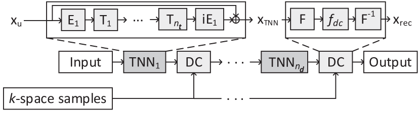
(a) $\mathbf{E}$ is the token embedding and $i\mathbf{E}$ its inverse, $\mathbf{F}$ is the DFT, $n_{t}$ are the number of transformer encoder layers per-TNN, $n_{d}$ are the number of cascaded TNN blocks and $f_{dc}$ is data consistency.

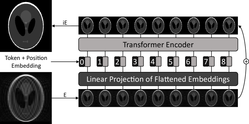
(b) Example of a ViT-based TNN denoiser with KD. Patch, KD and axial tokens are used in this work.

Fig. 2: Architecture for the proposed DcTNN.

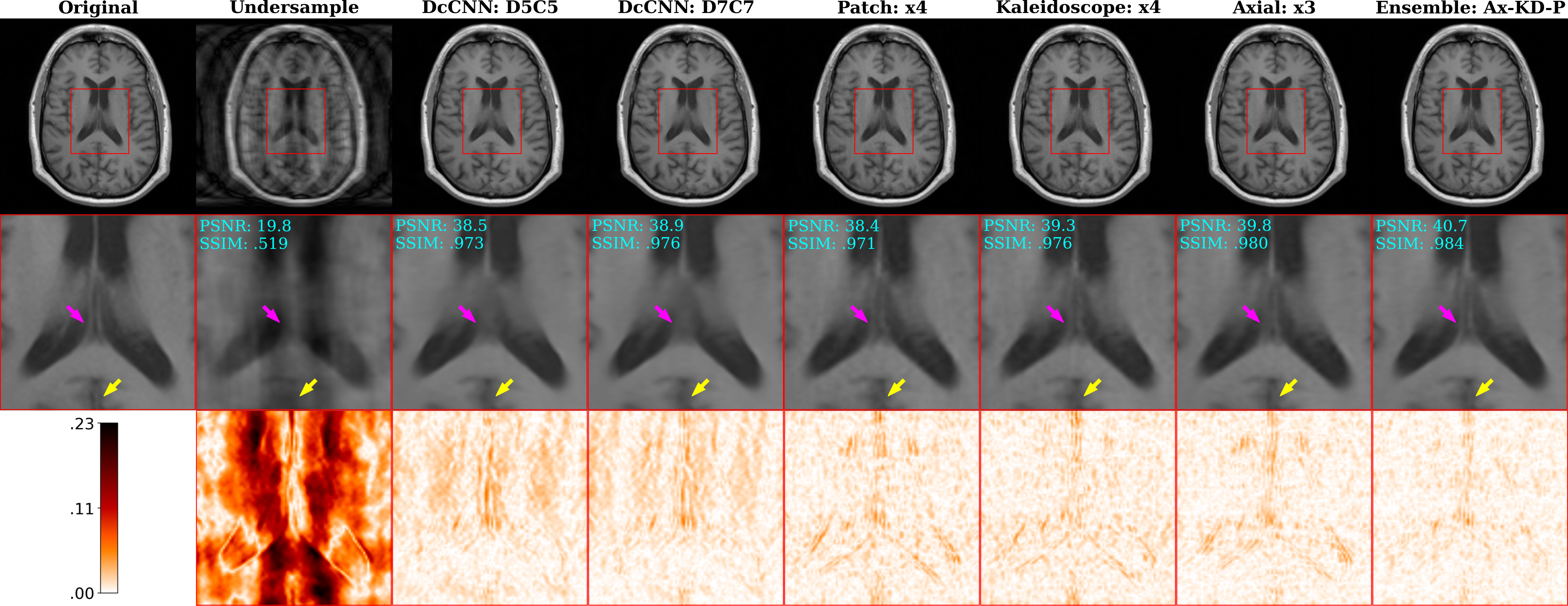
Fig. 3: Reconstruction performance demonstrated at R6 reduction factor of a cross-sectional brain MR image, with the zoomed area (red rectangle) including the region of the right and left lateral ventricle. Patch and Kaleidoscope DcTNN are comprised of 4 TNN layers. Axial and Ensemble: Ax-KD-P each have 3. Finally, DcCNN are the reference [9]. Values $\in[0,1]$.

2.2 Network Architecture

In order to effectively deploy ViT for CS-MRI, we impose two major architectural considerations. Firstly, TNN blocks should be introduced in a cascaded manner. Secondly, efficient gradient back-propagation is required given the large number of parameters in TNN. This study extends on the DcCNN as it comprises a relatively simple network architecture that is suitable to these conditions (see Fig. 2(a)). DcCNN solves the following CS optimisation problem,

$$\min_{\mathbf{x,\theta}}\;\|\mathbf{x}-f(\mathbf{x})\|^{2}_{2}+\lambda\|\mathbf{\text{F}}_{u}\mathbf{x}-\mathbf{y}\|^{2}_{2},$$ (1)

where $\mathbf{x}$ is the predicted image, $\mathbf{y}$ is collected discrete Fourier samples, $\mathbf{F}_{u}$ is the Fourier under-sampling operator, and $f$ regularises the solution. When solved analytically, image estimates $\mathbf{\hat{x}}$ are produced by iteratively applying and adapting $f$ during the reconstruction process [14]. DcCNN instead replaces $f$ with $f_{cnn,\mathbf{\theta}}$, therefore learning an optimal denoising between iterations in a deep manner; $\mathbf{\theta}$ are the CNN parameters. As has been discussed, CNNs suffer from inherent limitations that have been overcome by TNNs in various applications. We therefore postulate that replacing $f_{cnn,\theta}$ with $f_{tnn,\theta}$ will result in superior image quality, with performance that better scales with available data and total number of parameters. Similarly to DcCNN, this Deep cascade of Transformer Neural Networks (DcTNN) features denoising (TNN) and data consistency (DC) blocks.

TNN Denoiser: DcCNN utilises CNN denoiser blocks that feature a number of convolutional layers $n_{c}$, and filters $n_{f}$. Instead, we employ TNN blocks with $n_{t}$ transformer encoder layers, as-well as an embedding layer $\mathbf{E}$. This embedding can either be common between TNN layers, or unique for each. In this way, arbitrary token embeddings such the proposed KD can be utilised for ViT (see Fig. 2(b)). Our implementation also uses learned positional embeddings.

We produce a multi-scale perceptive ViT by cascading TNN denoiser blocks with different token embedding types. In this “ensemble” design, each TNN block can specialise on the type of denoising based on its input features. The ensemble network cascades Axial (Ax), Kaleidoscope (KD), and Patch (P) TNN denoising blocks, with Table 1 summarising the image features each token attends to. We demonstrate the relative performance improvements afforded by combining these tokens for CS-MRI in Table 2 and Fig. 3.

Data Consistency: We implement DC blocks that execute:

$$f_{dc}(\mathbf{\hat{X}},\mathbf{y},\lambda)=\begin{cases}\mathbf{\hat{X}}(k)&\text{if $k\notin\Omega$}\\ \frac{\mathbf{\hat{X}}(k)+\lambda\mathbf{y}(k)}{1+\lambda}&\text{if $k\in\Omega$}\end{cases}$$ (2)

Here $\mathbf{\hat{X}}$ are the discrete Fourier coefficients of the current image estimate $\mathbf{\hat{x}}$, $\lambda$ is a weighting parameter and $\Omega$ represents the subset of sampled points $\mathbf{y}$ with $k$ being an index. In the noiseless case, $\lambda\rightarrow\infty$, and $k\in\Omega$ are directly replaced by $\mathbf{y}$. In our testing, we found that setting $\lambda$ as a learnable parameter in each DC block improved performance for DcTNN. However, DcCNN performed best in the noiseless case.

Table 1: Relative scales of Vision.

Token	Image Scale	Frequency Scale
Axial	Local	Low, High
KD	Global	Low
Patch	Local	High
Ensemble: Ax-KD-P	Local, Global	Low, High

Table 2: Average reconstruction performance, number of parameters for tested networks and associated training information. Bold and underline indicate best and second best outcomes respectively.

	Denoising		R=4			R=6			R=8			Number of	Minutes
Method	Blocks		PSNR	SSIM		PSNR	SSIM		PSNR	SSIM		Parameters	Per-Epoch
D5C5 [9]	5		45.61	0.99		41.31	0.97		37.68	0.96		0.14M	14.7
D7C7 [9]	7		46.47	0.99		41.94	0.98		37.85	0.96		1.3M	91.8
Patch	4		42.68	0.98		41.43	0.98		37.31	0.96		29.3M	5.8
Kaleidoscope	4		43.48	0.98		41.84	0.98		37.54	0.96		29.3M	5.8
Axial	3		44.75	0.99		42.30	0.98		38.19	0.97		38.5M	5.5
Ensemble	3		45.01	0.99		42.99	0.98		38.55	0.97		27.5M	4.6

3 Results and Discussion

Experimental Configuration: A subset of the NYU fastMRI DICOM brain database was used to train and test models, constituting $64,180$ T1-w cross-sectional MR images [15]. Training, validation and testing consisted of 80%, 10% and 10% of these images. We simulate single-coil magnitude images and cropped each to $320\times 320$ resolution. Discrete Fourier space was sampled using a 1D Gaussian random mask. Closeness to the original image is measured with peak signal-to-noise ratio (PSNR) and structural similarity (SSIM). DcTNN networks employ $n_{t}=2$, where patch and KD are $16\times 16$ and $d_{model}=256$; $d_{model}=320$ for axial tokens. D5C5 DcCNN features $5$ CNN blocks with $n_{c}=5$ and $n_{f}=32$. D7C7 instead has $7$ CNN blocks with $n_{c}=7$ and $n_{f}=64$. Further details regarding the training and testing methodology are included in the supplementary material.

Qualitative Analysis: Fig. 3 illustrates the reconstruction characteristics of both DcTNN and DcCNN methods. The arrows point to regions of faint, noise-like image features that all DcTNN are able to recover; DcCNN over-smooths such regions. Although individual patch, KD and axial DcTNN leave similar residual artefacts, ensemble (Ax-KD-P) is capable of accurately discerning the underlying image. Additionally, the ensemble network is more faithful to the original image textures compared to DcCNN. These reconstruction characteristics are persistent for all reduction factors tested. In fact, despite DcCNN scoring higher PSNR and SSIM at R4 (Table 2), image features such as those portrayed in Fig. 3 still lack significant recovery. Visual comparisons at R4 and R8 are available in the supplementary material.

Quantitative Analysis: We evaluated the reconstruction performance of our DcTNN at several under-sampling rates and compared the results to DcCNN in Table 2. We found that a DcTNN composed entirely of KD embeddings outperforms an equivalent patch-based approach, behaving similarly to the axial case; the axial network required more parameters. Importantly, the ensemble of cascaded axial, KD and patch TNN notably reduces the number of parameters required whilst achieving the highest PSNR and SSIM scores. Further, training time per-epoch is just a fraction of that required for CNN alternatives. These results indicate that our ensemble DcTNN is most capable of recovering image information at higher reduction factors, i.e., R6 and R8. It also highlights that the combination of token embeddings can be effectively leveraged for multi-scale processing, resulting in smaller and more efficient networks.

Fig. 4 illustrates the comparative training characteristics of the DcTNN methods. Here, we see the naive patch-based approach requires many epochs for convergence. At the same number of parameters, KD is able to converge faster, and to a lower loss value. While the axial network requires more parameters, overall convergence is similar to that attained with KD. Finally, the ensemble network achieves the lowest overall validation loss, as-well as the fastest convergence. These findings demonstrate that KD surpasses image patches at efficiently modelling input characteristics. The ensemble network further benefits from the many image scales presented as inputs throughout reconstruction.

4 Conclusion

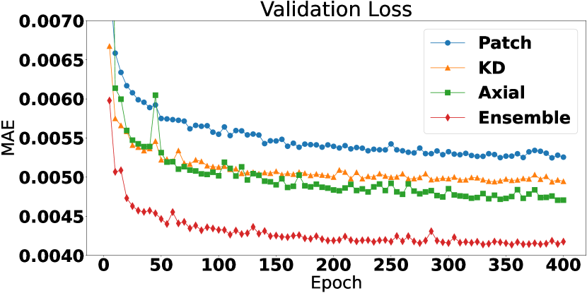
Fig. 4: DcTNN validation loss (MAE) at R6. Ensemble demonstrates superior convergence.

This paper has demonstrated the benefits afforded by our novel Kaleidoscope token (KD) embeddings, which provides low frequency, global image representations. Their use for CS-MRI improved training and reconstruction characteristics compared to image patches due to superior modelling of global features such as CS artefacts. We also present the advantages of cascading token types, therefore encouraging TNN layers to specialise at “seeing” particular image features. This combined approach ensures a multi-scale perceptive ViT without a reduction of resolution, or necessitating a windowed approach that may reduce overall vision scales.

Future work should investigate convolutions within DcTNN, as CNN are known to improve training characteristics of ViT. We also theorise that the total number of parameters can be reduced via the KT. In this proposed configuration, low-resolution copies of the image can be attended to separately without reducing vision scales. In conclusion, the advantages of utilising more than a single form of token embedding has been demonstrated, with our novel KD producing promising results. We propose that similar tokenisation can be successfully employed in many other fields of CV.

References

- [1] Ashish Vaswani, Noam Shazeer, Niki Parmar, Jakob Uszkoreit, Llion Jones, Aidan N Gomez, Łukasz Kaiser, and Illia Polosukhin, “Attention is All you Need,” in Advances in Neural Information Processing Systems. 2017, vol. 30, Curran Associates, Inc.
- [2] Alexey Dosovitskiy, Lucas Beyer, Alexander Kolesnikov, Dirk Weissenborn, Xiaohua Zhai, Thomas Unterthiner, Mostafa Dehghani, Matthias Minderer, Georg Heigold, Sylvain Gelly, Jakob Uszkoreit, and Neil Houlsby, “An image is worth 16x16 words: Transformers for image recognition at scale,” in International Conference on Learning Representations, 2021.
- [3] Li Yuan, Yunpeng Chen, Tao Wang, Weihao Yu, Yujun Shi, Zi-Hang Jiang, Francis E.H. Tay, Jiashi Feng, and Shuicheng Yan, “Tokens-to-token vit: Training vision transformers from scratch on imagenet,” in Proceedings of the IEEE/CVF International Conference on Computer Vision (ICCV), October 2021, pp. 558–567.
- [4] Haoqi Fan, Bo Xiong, Karttikeya Mangalam, Yanghao Li, Zhicheng Yan, Jitendra Malik, and Christoph Feichtenhofer, “Multiscale vision transformers,” in Proceedings of the IEEE/CVF International Conference on Computer Vision (ICCV), October 2021, pp. 6824–6835.
- [5] Ze Liu, Yutong Lin, Yue Cao, Han Hu, Yixuan Wei, Zheng Zhang, Stephen Lin, and Baining Guo, “Swin transformer: Hierarchical vision transformer using shifted windows,” in Proceedings of the IEEE/CVF International Conference on Computer Vision (ICCV), October 2021, pp. 10012–10022.
- [6] Jonathan Ho, Nal Kalchbrenner, Dirk Weissenborn, and Tim Salimans, “Axial Attention in Multidimensional Transformers,” arXiv e-prints, p. arXiv:1912.12180, Dec. 2019.
- [7] Tete Xiao, Piotr Dollar, Mannat Singh, Eric Mintun, Trevor Darrell, and Ross Girshick, “Early convolutions help transformers see better,” in Advances in Neural Information Processing Systems, A. Beygelzimer, Y. Dauphin, P. Liang, and J. Wortman Vaughan, Eds., 2021.
- [8] Jeya Maria Jose Valanarasu, Poojan Oza, Ilker Hacihaliloglu, and Vishal M. Patel, “Medical Transformer: Gated Axial-Attention for Medical Image Segmentation,” in Medical Image Computing and Computer Assisted Intervention – MICCAI 2021, Marleen de Bruijne, Philippe C. Cattin, Stéphane Cotin, Nicolas Padoy, Stefanie Speidel, Yefeng Zheng, and Caroline Essert, Eds., Cham, 2021, Lecture Notes in Computer Science, pp. 36–46, Springer International Publishing.
- [9] Jo Schlemper, Jose Caballero, Joseph V. Hajnal, Anthony Price, and Daniel Rueckert, “A Deep Cascade of Convolutional Neural Networks for MR Image Reconstruction,” in Information Processing in Medical Imaging, Marc Niethammer, Martin Styner, Stephen Aylward, Hongtu Zhu, Ipek Oguz, Pew-Thian Yap, and Dinggang Shen, Eds., Cham, 2017, Lecture Notes in Computer Science, pp. 647–658, Springer International Publishing.
- [10] Jacob M. White, Stuart Crozier, and Shekhar S. Chandra, “Bespoke Fractal Sampling Patterns for Discrete Fourier Space via the Kaleidoscope Transform,” IEEE Signal Processing Letters, vol. 28, pp. 2053–2057, 2021, IEEE Signal Processing Letters.
- [11] Shekhar S. Chandra, Gary Ruben, Jin Jin, Mingyan Li, Andrew M. Kingston, Imants D. Svalbe, and Stuart Crozier, “Chaotic Sensing,” IEEE Transactions on Image Processing, vol. 27, no. 12, pp. 6079–6092, Dec. 2018, IEEE Transactions on Image Processing.
- [12] Michael Elad and Michal Aharon, “Image denoising via sparse and redundant representations over learned dictionaries,” IEEE Transactions on Image Processing, vol. 15, no. 12, pp. 3736–3745, 2006.
- [13] Christopher A. Metzler, Arian Maleki, and Richard G. Baraniuk, “From denoising to compressed sensing,” IEEE Transactions on Information Theory, vol. 62, no. 9, pp. 5117–5144, 2016.
- [14] Saiprasad Ravishankar and Yoram Bresler, “MR Image Reconstruction From Highly Undersampled k-Space Data by Dictionary Learning,” IEEE Transactions on Medical Imaging, vol. 30, no. 5, pp. 1028–1041, May 2011, IEEE Transactions on Medical Imaging.
- [15] Jure Zbontar, Florian Knoll, Anuroop Sriram, Tullie Murrell, Zhengnan Huang, Matthew J. Muckley, Aaron Defazio, Ruben Stern, Patricia Johnson, Mary Bruno, Marc Parente, Krzysztof J. Geras, Joe Katsnelson, Hersh Chandarana, Zizhao Zhang, Michal Drozdzal, Adriana Romero, Michael Rabbat, Pascal Vincent, Nafissa Yakubova, James Pinkerton, Duo Wang, Erich Owens, C. Lawrence Zitnick, Michael P. Recht, Daniel K. Sodickson, and Yvonne W. Lui, “fastMRI: An Open Dataset and Benchmarks for Accelerated MRI,” 2019.