MU-MIMO Receiver Design and Performance Analysis in Time-Varying Rayleigh Fading

On the Achievable SINR in MU-MIMO Systems Operating in Time-Varying Rayleigh Fading

Abstract

Minimizing the symbol error in the uplink of multi-user multiple input multiple output systems is important, because the symbol error affects the achieved signal-to-interference-plus-noise ratio (SINR) and thereby the spectral efficiency of the system. Despite the vast literature available on minimum mean squared error (MMSE) receivers, previously proposed receivers for block fading channels do not minimize the symbol error in time-varying Rayleigh fading channels. Specifically, we show that the true MMSE receiver structure does not only depend on the statistics of the CSI error, but also on the autocorrelation coefficient of the time-variant channel. It turns out that calculating the average SINR when using the proposed receiver is highly non-trivial. In this paper, we employ a random matrix theoretical approach, which allows us to derive a quasi-closed form for the average SINR, which allows to obtain analytical exact results that give valuable insights into how the SINR depends on the number of antennas, employed pilot and data power and the covariance of the time-varying channel. We benchmark the performance of the proposed receiver against recently proposed receivers and find that the proposed MMSE receiver achieves higher SINR than the previously proposed ones, and this benefit increases with increasing autoregressive coefficient.

I Introduction

The wireless channels in the uplink of multiuser multiple input multiple output (MU-MIMO) systems can often be advantageously modelled as autoregressive (AR) processes, because AR channel models capture the time-varying (aging) nature of the channels and facilitate channel estimation and prediction [1, 2, 3, 4, 5, 6, 7, 8, 9, 10, 11, 12, 13]. These papers have shown that exploiting the autoregressive structure of the time-varying Rayleigh fading channel improves the performance of both single input single output (SISO) and multiple input multiple output (MIMO) channel estimators and receivers. The basic rationale for these papers is that in a Rayleigh fading environment, based on the associated Jakes process, an AR model can be built, which allows one to employ Kalman filters for estimating and predicting the channel state. Specifically, papers [2], and [4, 5, 6] consider SISO systems and exploit the memoryful property of the AR process for joint channel estimation, equalization and data detection.

Some early works on multiple-antenna receiver design and performance analysis are reported in [1] and [3]. The optimal array receiver algorithm for binary phase-shift keying (BPSK) signals is designed in [1], while reference [3] is concerned with the blind estimation and detection of space-time coded symbols transmitted over time-varying Rayleigh fading channels. More recently, in the context of massive MU-MIMO systems, [7, 8, 9, 10, 11, 12, 13] addressed the problem of channel aging and derived channel estimation, prediction and multi-user receiver algorithms that operate in an AR Rayleigh-fading environment and use Kalman filters or machine learning algorithms for channel prediction.

Table I: Overview of Related Literature

Reference	UL or DL	Channel model and channel estimation	Perf. Indicator	Is asymptotic random matrix theory (RMT) used ?	Comment
Couillet et al., [14]	MIMO MAC	block fading, channel estimation (CE) out of scope (OoS)	rate region, rate maximization	Yes	receiver design OoS
Hanlen et al., [15]	UL/DL	block fading with correlated MIMO channels, perfect CSI at receiver	capacity	Yes	receiver design OoS
Couillet et al., [16]	UL/DL	block fading, CE is OoS	capacity and sum-rate	Yes	receiver design OoS
Wen et al., [17]	MIMO MAC	block fading, non-Gaussian, CE is OoS	ergodic mutual information	Yes	receiver design OoS
Hoydis et al., [18]	UL/DL	block fading, MMSE CE	achievable rate	Yes	regularized MMSE receiver that takes into account the estimated channels of all users
Truong et al., [7]	UL/DL	AR(p), AR(1), MMSE, channel prediction	average SINR, achievable rate	Yes	MRC receiver (not AR-aware)
Kong et al., [8]	UL/DL	similar to that in [7]	UL/DL average rate	Yes	MRC and ZF receivers (not AR-aware)
Papazafeiropoulos et al., [19]	UL	AR(1), MMSE estimation	average SINR, outage probability	Yes	MRC receiver, UL caching
Björnson et al., [20]	UL/DL	block fading, multicell MMSE CE	average SINR, spectral efficiency	Yes	multicell MMSE receiver
Boukhedini et al., [21]	UL/DL	block fading, multicell MMSE CE	average SINR, spectral efficiency	Yes	multicell MMSE receiver
Sanguinetti et al., [22]	UL/DL	block fading, multicell MMSE CE	average SINR, spectral efficiency	Yes	multicell MMSE receiver
Yuan et al., [12]	UL/DL	AR(1), ML-based prediction	channel estimation/prediction quality (MSE)	No	receiver design OoS (focus on channel estimation/prediction)
Abrardo et al., [23]	UL	block fading, LS CE	MSE and SINR	Yes	MMSE receiver for block fading channels is derived; takes into account the estimated channels of all users
Kim et al., [11]	UL/DL	3GPP spatial channel model, ML-based and Kalman filter-based prediction, mobility prediction	channel estimation/prediction quality (MSE)	No	receiver design OoS (focus on channel estimation/prediction)
Fodor et al., [13]	UL	AR(1), Kalman filter-based channel estimation	MSE of received data symbols	No	regularized (AR-aware) MMSE receiver, regularization is based on covariance matrices, interference is treated as nosie
Chopra and Murthy [24]	UL/DL	AR($p$), Kalman filter-based and data assisted channel estimation	MSE of the channel estimation and received data symbols, and achievable rate	Yes	AR-aware MMSE receiver that utilizes data-aided channel tracking
Present paper	UL	AR(1), Kalman filter-based channel estimation	average SINR, average rate	Yes	new MMSE receiver, whose structure takes into account the AR parameters and estimated channels of all users

A closely related line of research, in block fading environments, applies results from random matrix theory to establish the deterministic equivalent of the random wireless system in order to calculate the signal-to-interference-plus-noise ratio (SINR) in the uplink and downlink of MU-MIMO systems [14, 15, 16, 17, 18, 25, 26, 19, 20, 21, 23, 22]. In particular, in papers [20, 21, 22] it was shown that the capacity of multicell MU-MIMO networks grows indefinitely as the number of antennas tends to infinity, if appropriate multicell minimum mean squared error (MMSE) processing is used.

Generalizing the downlink (DL) precoding and uplink (UL) receiver structures and associated deterministic equivalent SINR results developed in these papers to AR time-varying environments and channel aging is not trivial, because of the basic assumption on independent channel realizations at subsequent time instances. In contrast, papers [7, 8, 19, 11, 12] treat AR channel evolution and use random matrix theory to derive the deterministic equivalent and thereby the SINR for the UL and DL of MU-MIMO systems. However, these papers do not develop a MU-MIMO receiver that aims to minimize the mean squared error (MSE) of the received data symbols. More recently, paper [24] developed a data-aided MSE-optimal channel tracking scheme and associated MMSE estimator of the data symbols in the presence of channel aging, that is when the channel changes between the channel estimation time instance and the time instance when the channel is used for data transmission.

In our recent work [13], we developed a new MMSE receiver that treats interference as noise and uses an AR model for its performance analysis (see Table I). The important conclusion in [13] is that not only the channel estimation procedure, but the receiver structure itself should be modified when the fading process is AR.

However, it is well-known that treating interference as noise in MU-MIMO systems can severely degrade the performance as compared with using the instantaneous channel estimates of the interfering users, see the UL MU-MIMO receiver structures used in, for example, [18, 7, 8, 23]. Specifically, papers [18] and [23] proposed MMSE receivers in block fading, whereas a maximum ratio combining (MRC) and zero-forcing (ZF) receiver in time-varying channels in the presence of channel aging are used by [7] and [8] respectively. Note that the conceptual difference between the MRC and ZF receivers used in [7] and [8] and the MMSE receiver proposed in [13] lies in the fact that the MMSE receiver actively takes into account that the subsequent channel realizations are correlated rather than adopting the MMSE receiver structure developed for block fading channels. Therefore, we refer to the MMSE receiver in [13] as an AR-aware receiver.

In the light of these works, it is natural to ask the following two questions:

• What is the MU-MIMO receiver that minimizes the MSE of the received data symbols in time-varying Rayleigh fading when all user channels are estimated and, therefore, the multiuser interference does not need to be treated as noise?

• Can we calculate the average SINR in the uplink of MU-MIMO systems that employ the above receiver, as a function of the number of MU-MIMO users and receive antennas, employed pilot and data powers and large scale fading?

Intuitively, finding the answers to these questions implies extending the results by (1) papers [18] and [23] (by generalizing some of those block fading results to AR processes), (2) papers [7] and [8] (by developing the optimal linear receiver in MSE sense) and (3) paper [13] (by not treating the MU-MIMO interference as noise and deriving an SINR formula rather than using the MSE as a performance metric). Consequently, the objective of the present paper is to devise a MU-MIMO receiver that utilizes the channel estimates of each user and the fact that subsequent channel coefficients are correlated in time. In other words, we propose and analyze a MU-MIMO receiver that is optimal in the presence of channel state information (CSI) errors when the channel evolves in time according to a Rayleigh fading autocorrelation process. It is also our objective to derive an average SINR formula that can serve as a basis for rate optimization schemes in future works. Thus, our contributions to the existing literature summarized above and in Table I are two-fold:

1. Calculating the deterministic equivalent SINR of the MU-MIMO MMSE receiver proposed in Proposition 1, by proving Proposition 2, Theorem 2, whose proof is based on Theorem 1 and Corollary 1, is our main and novel result. To the best of our knowledge, Theorem 1, Lemma 4 (needed for Theorem 1) and Theorem 2 have not been published before.

2. We would like to emphasize the usefulness of Proposition 3, which gives a straightforward computation of the optimum pilot power in a MU-MIMO AR Rayleigh fading environment as a root of a quartic equation.

Our analytical (based on Theorem 2 and Proposition 3) and simulation results (comparing the performance of the different MU-MIMO receivers listed in Table IV) indicate that the proposed AR-aware receiver outperforms earlier AR receivers in terms of the achieved SINR, such as those proposed by Truong and Heath [7] and our own previously proposed scheme in [13].

The paper is organized as follows. The next section describes our system model, which is similar to that used in, for example [13], [18] or [7]. Section III derives the MMSE receiver for autoregressive Rayleigh fading channels, stated as Proposition 1. Section IV derives our key result, Theorem 2, which can be considered as an extension of the SINR results in [18] and [23] to AR processes. The important feature of this implicit SINR formula is that it does not require to solve a system of equations or fixed point iterations due to the fact that the implicit equation has a unique positive solution. Also, Subsection IV-D derives the optimum pilot power in single-user multiple input multiple output (SU-MIMO) systems or in MU-MIMO systems, in the special case when the large scale fading components of all users are equal. The treatment of the optimum pilot power in the general MU-MIMO case is left for future work. Section V discusses numerical results, and Section VI draws conclusions.

II System Model

II-A Uplink Signal Model

We consider a single cell MU-MIMO system, where the base station (BS) is equipped with $N_{r}$ receive antennas, and there are $K$ uplink mobile stations. (Note that typically $K\ll N_{r}$.) The MSs facilitate channel state information at the receiver (CSIR) acquisition at the BS using orthogonal complex sequences, such as the Zadoff-Chu sequences, defined as $\mathbf{s}\triangleq\left[s_{1},...,s_{\tau_{p}}\right]^{T}\in\mathds{C}^{{\tau_{p}\times 1}}$. These pilot sequences satisfy $|s_{i}|^{2}=1$, for $i=1,..,\tau_{p}$ [27]. To enable spatial multiplexing, the length of the pilot sequences $\tau_{p}$ is chosen such that a maximum of $K$ users can be served simultaneously, implying that $\tau_{p}\geq K$ holds. In this MU-MIMO system, $\tau_{p}$ subcarriers are used to construct the pilot sequences at each MS, and $\tau_{d}$ subcarriers are used to transmit data symbols. Each MS has a total power budget $P_{\text{tot}}$, imposing the constraint $\tau_{p}P_{p}+\tau_{d}P=P_{\text{tot}}$, where $P$ is the transmit and $P_{p}$ denotes the pilot power. The trade-off between pilots and data signals as implied by the sum pilot and data power constraint has been studied by several previous works, see for example [28, 29]. In this paper, User-1 is the tagged user, while indexes $2\ldots K$ are used to denote the interfering users from the tagged user’s point of view. Consequently, the received pilot signal transmitted by User-1 at the BS takes the form of [13]:

$$\mathbf{Y}^{p}(t) =\alpha\sqrt{P_{p}}\mathbf{h}(t)\mathbf{s}^{T}+\mathbf{N}(t)\leavevmode\nobreak\ \leavevmode\nobreak\ \in\mathds{C}^{N_{r}\times\tau_{p}},$$ (1)

where $\mathbf{h}(t)\leavevmode\nobreak\ \in\leavevmode\nobreak\ \mathds{C}^{N_{r}\times 1}\sim\mathcal{CN}(\mathbf{0},\mathbf{C})$, that is, $\mathbf{h}(t)$ is a complex normal distributed column vector with mean vector $\mathbf{0}$ and covariance matrix $\mathbf{C}$. Furthermore, $\alpha$ denotes large scale fading, and $\mathbf{N}\in\mathds{C}^{N_{r}\times\tau_{p}}$ is the additive white Gaussian noise (AWGN) with element-wise variance $\sigma_{p}^{2}$.

II-B Channel Model

In this paper $\mathbf{h}$ denotes the complex channel which is modeled as a stationary discrete time AR(1) process as in [4, 5, 13]. This model can be seen as a generalization of the block fading channel model: $\mathbf{h}(t)=\mathbf{A}\mathbf{h}(t-1)+\bm{\vartheta}(t)\quad\in\mathds{C}^{N_{r}\times 1}$, where $\bm{\vartheta}(t)\sim\mathcal{CN}\left(\mathbf{0},\bm{\Theta}\right)$ is the process noise vector and $\mathbf{A}$ denotes the state transition matrix of the AR(1) process [3]. In this paper we will use this AR(1) model to approximate the Rayleigh fading channel. We remark that the parameters of the AR(1) model can be identified by existing methods, such as those reported in [30, 31] and [32]. Due to the stationarity of $\mathbf{h}(t)$ we have $\mathbf{C}=\mathbf{A}\mathbf{C}\mathbf{A}^{H}+\bm{\Theta}$.

II-C Data Signal Model

Table II: System Parameters

Notation	Meaning
$K$	Number of MU-MIMO users
$N_{r}$	Number of antennas at the BS
$\tau_{p},\tau_{d}$	Number of pilot/data symbols within a coherent set of subcarriers
$\mathbf{s}\in\mathds{C}^{\tau_{p}\times 1}$	Sequence of pilot symbols
$x$	Data symbol
$P_{p},P,P_{\text{tot}}$	Pilot power per symbol, data power per symbol, and total power budget
$\mathbf{Y}^{p}\in\mathds{C}^{N_{r}\times\tau_{p}},y(t)\in\mathds{C}^{N_{r}}$	Received pilot and data signal, respectively
$\mathbf{h}(t),\hat{\mathbf{h}}(t)\in\mathds{C}^{N_{r}}$	Fast fading channel and estimated channel
$\mathbf{A}\in\mathds{C}^{N_{r}\times N_{r}}$	AR parameter of the channel
$\bm{\vartheta}(t)\in\mathds{C}^{N_{r}},\bm{\Theta}\in\mathds{C}^{N_{r}\times N_{r}}$	Process noise of the channel AR process and its covariance matrix
$\bm{\varepsilon}(t)\in\mathds{C}^{N_{r}},\bm{\Sigma}\in\mathds{C}^{N_{r}\times N_{r}}$	Channel estimation error and its covariance matrix
$\mathbf{G},\mathbf{G}^{\text{naive}},\mathbf{G}^{\star}$	MU-MIMO receivers: generic, naive, and optimal, respectively.

Considering $K$ MU-MIMO users, the received data signal at the BS at time $t$ is [13]:

$$\mathbf{y}(t) =\underbrace{\mathbf{\alpha}\mathbf{h}(t)\sqrt{P}x(t)}_{\text{tagged user}}+\underbrace{\sum_{k=2}^{K}\mathbf{\alpha}_{k}\mathbf{h}_{k}(t)\sqrt{P_{k}}x_{k}(t)}_{\text{other users}}+\mathbf{n}_{d}(t),$$ (2)

where $\mathbf{y}(t)\in\mathds{C}^{N_{r}\times 1}$; and $\mathbf{\alpha}_{k}\mathbf{h}_{k}(t)\in\mathds{C}^{N_{r}\times 1}$ denotes the channel vector, and $x_{k}(t)$ is the data symbol of User-$k$ transmitted at time $t$ with power $P_{k}$. Furthermore $\mathbf{n}_{d}(t)\leavevmode\nobreak\ \sim\mathcal{CN}\left(\mathbf{0},\sigma_{d}^{2}\mathbf{I}_{N_{r}}\right)$ is the AWGN, where $\mathbf{I}_{N_{r}}$ denotes the identity matrix of size $N_{r}$.

II-D Channel Estimation

To acquire CSIR, the MSs transmit orthogonal pilot sequences, and the BS uses MMSE channel estimation based on (1). For algebraic convenience we define

$$\mathbf{\tilde{Y}}^{p}(t)=\textbf{vec}\left(\mathbf{Y}^{p}(t)\right)=\alpha\sqrt{P_{p}}\mathbf{S}\mathbf{h}(t)+\mathbf{\tilde{N}}(t){\color[rgb]{0,1,1}{,}}$$ (3)

where vec is the column stacking vector operator, $\mathbf{\tilde{Y}}^{p}(t),\mathbf{\tilde{N}}(t)\in\mathds{C}^{\tau_{p}N_{r}\times 1}$ and $\mathbf{S}\triangleq\mathbf{s}\otimes\mathbf{I}_{N_{r}}\in\tau_{p}N_{r}\times N_{r}$) is such that $\mathbf{S}^{H}\mathbf{S}=\tau_{p}\mathbf{I}_{N_{r}}$.

Lemma 1.

The MMSE channel estimator approximates the AR(1) channel based on the latest and the previous channel states as

$$\mathbf{\hat{h}}_{\textup{MMSE}}(t) =\begin{bmatrix}\mathbf{C}&\mathbf{A}\mathbf{C}\end{bmatrix}\left(\frac{\sigma_{p}^{2}}{\alpha^{2}P_{p}\tau_{p}}\mathbf{I}_{2N_{r}}+\mathbf{M}\right)^{-1}$$

$$\leavevmode\nobreak\ \leavevmode\nobreak\ \leavevmode\nobreak\ \leavevmode\nobreak\ \left(\mathbf{\bar{h}}(t)+\frac{1}{\alpha\sqrt{P_{p}}\tau_{p}}\mathbf{\bar{n}}(t)\right),$$ (4)

where $\mathbf{M}=\begin{bmatrix}\mathbf{C}&\mathbf{A}\mathbf{C}\\ \mathbf{C}\mathbf{A}^{H}&\mathbf{C}\end{bmatrix}$, $\mathbf{\bar{h}}(t)=\begin{bmatrix}\mathbf{h}(t)\\ \mathbf{h}(t-1)\end{bmatrix}$   and
$\text{\leavevmode\nobreak\ \leavevmode\nobreak\ \leavevmode\nobreak\ }\mathbf{\bar{n}}(t)=\begin{bmatrix}\mathbf{s}^{H}\mathbf{N}(t)\\ \mathbf{s}^{H}\mathbf{N}(t-1)\end{bmatrix}$.

The proof is in Appendix A.

Corollary 1.

The estimated channel $\mathbf{\hat{h}}_{\textup{MMSE}}$ is a circular symmetric complex normal distributed vector $\mathbf{\hat{h}}_{\textup{MMSE}}(t)\sim\mathcal{CN}(\mathbf{0},\mathbf{R}_{\textup{MMSE}})$, with

$$\mathbf{R}_{\textup{MMSE}} =\mathds{E}_{\mathbf{h},\mathbf{n}}\{\mathbf{\hat{h}}_{\textup{MMSE}}(t)\mathbf{\hat{h}}_{\textup{MMSE}}^{H}(t)\}$$

$$=\begin{bmatrix}\mathbf{C}&\mathbf{A}\mathbf{C}\end{bmatrix}\left(\frac{\sigma_{p}^{2}}{\alpha^{2}P_{p}\tau_{p}}\mathbf{I}_{2N_{r}}+\mathbf{M}\right)^{-1}\begin{bmatrix}\mathbf{C}\\ \mathbf{C}\mathbf{A}^{H}\end{bmatrix}$$ (5)

$$=\left[\begin{array}[]{ccc}\mathbf{C}&\mathbf{AC}\end{array}\right]\left[\begin{array}[]{ccc}\mathbf{C}+\mathbf{\Sigma}&\mathbf{AC}\\ \mathbf{C}\mathbf{A}^{H}&\mathbf{C}+\mathbf{\Sigma}\end{array}\right]^{-1}\left[\begin{array}[]{ccc}\mathbf{C}\\ \mathbf{C}\mathbf{A}^{H}\end{array}\right],$$ (11)

where $\mathbf{\Sigma}\triangleq\frac{\sigma_{p}^{2}}{\alpha^{2}P_{p}\tau_{p}}\mathbf{I}_{N_{r}}$.

We note that (1) is obtained from (1) using $\mathds{E}_{\mathbf{h},\mathbf{n}}\{\mathbf{\bar{h}}(t)\mathbf{\bar{h}}(t)^{H}\}=\mathbf{M}$ and $\mathds{E}_{\mathbf{h},\mathbf{n}}\{\mathbf{\bar{n}}(t)\mathbf{\bar{n}}(t)^{H}\}=\tau_{p}\sigma_{p}^{2}\mathbf{I}_{2N_{r}}$. According to Corollary 1 and $\mathbf{h}(t)\sim\mathcal{CN}(\mathbf{0},\mathbf{C})$, the covariance matrix of the channel estimation noise when using the MMSE channel estimation is: $\mathbf{Z}=\mathbf{C}-\mathbf{R}_{\textrm{MMSE}}$, which is identical with the LS case discussed in [13], and we therefore omit the MMSE subscript in the sequel.

Lemma 2.

The channel realization $\mathbf{h}(t)$ conditioned on the current and previous estimates $\mathbf{\hat{h}}(t)$ and $\mathbf{\hat{h}}(t-1)$ is normally distributed as follows:

$$\left(\mathbf{h}(t)\Big{|}\mathbf{\hat{h}}(t),\mathbf{\hat{h}}(t-1)\right) \sim\mathbf{E}\bm{\zeta}(t)+\underbrace{\mathcal{CN}\Big{(}\mathbf{0},\mathbf{Z}\Big{)}}_{\textup{channel estimation noise}},$$ (12)

where for $\forall t$

$$\bm{\zeta}(t)\triangleq\left[\begin{array}[]{ccc}\mathbf{\hat{h}}(t)\\ \mathbf{\hat{h}}(t-1)\end{array}\right]\in\mathds{C}^{2N_{r}\times 1},$$ (15)

$$\mathbf{E}\triangleq\left[\begin{array}[]{ccc}\mathbf{C}&\mathbf{AC}\end{array}\right]\left[\begin{array}[]{ccc}\mathbf{C}+\mathbf{\Sigma}&\mathbf{AC}\\ \mathbf{C}\mathbf{A}^{H}&\mathbf{C}+\mathbf{\Sigma}\end{array}\right]^{-1}\in\mathds{C}^{N_{r}\times 2N_{r}},$$ (19)

$$\mathbf{Z}\triangleq\mathbf{C}-\mathbf{E}\left[\begin{array}[]{ccc}\mathbf{C}\\ \mathbf{C}\mathbf{A}^{H}\end{array}\right]\in\mathds{C}^{N_{r}\times N_{r}},\textup{\leavevmode\nobreak\ and\leavevmode\nobreak\ \leavevmode\nobreak\ }$$ (22)

$$\textup{Cov}\Big{(}\bm{\zeta}(t)\Big{)}=\left[\begin{array}[]{cc}\mathbf{C+\Sigma}&\mathbf{AC}\\ \mathbf{CA^{H}}&\mathbf{C+\Sigma}\end{array}\right]\in\mathds{C}^{2N_{r}\times 2N_{r}}.\leavevmode\nobreak\ \leavevmode\nobreak\ \leavevmode\nobreak\ \leavevmode\nobreak\ \leavevmode\nobreak\ \leavevmode\nobreak\$$ (25)

The proof is in [13].

II-E Summary

This section described the system model consisting of a signal model and an MMSE channel estimation scheme. When the channel estimation is based on the current and previous channel observations (i.e. $\mathbf{\hat{h}}(t)$ and $\mathbf{\hat{h}}(t-1)$), the conditional distribution of $\mathbf{h}$ is complex normal with mean vector and covariance matrix according to Lemma 2, which serves as a starting point for deriving the optimal MU-MIMO receiver in the sequel.

III Deriving the MMSE Receiver for Time-Varying Rayleigh Fading Channels

The BS the transmitted data symbols by employing a linear MMSE receiver $\mathbf{G}\in\mathds{C}^{1\times N_{r}}$, which minimizes the MSE between the transmitted symbol $x$ and the estimated symbol $\mathbf{G}\mathbf{y}$:

$$\mathbf{G}^{\star} \triangleq\text{arg}\min_{\mathbf{G}}\mathds{E}_{\mathbf{h},\mathbf{n},x}\{|\mathbf{G}\mathbf{y}-x|^{2}\}\leavevmode\nobreak\ \leavevmode\nobreak\ \in\mathds{C}^{1\times N_{r}}.$$ (26)

When the BS employs a naive receiver, it assumes perfect channel estimation, and uses the estimated channel in place of the actual channel:

$$\mathbf{G}^{\text{naive}}=\alpha\sqrt{P}\mathbf{\hat{h}}^{H}(\alpha^{2}P\mathbf{\hat{h}}\mathbf{\hat{h}}^{H}+\sigma_{d}^{2}\mathbf{I}_{N_{r}})^{-1}.$$ (27)

As we shall see, the naive receiver fails to minimize the MSE.

Next, we derive the MMSE receiver vector $\mathbf{G}^{\star}$ that the receiver at the BS should use to minimize the MSE of the received data symbol $x$ of the tagged user based on the data signal $\mathbf{y}$. Since the BS can only use the estimated channels, the objective function of this minimization must only depend on the estimated channels $\mathbf{\hat{h}}(t)$ and $\mathbf{\hat{h}}(t-1)$. This MMSE receiver can be contrasted to the naive receiver, which assumes that perfect CSIR is available.

The MSE of the received data symbols, as a function of the generic linear receiver $\mathbf{G}$ and the actual propagation channels $\mathbf{h}$, was shown to have the following form [33]:

$$\text{MSE}\big{(}\mathbf{G},\mathbf{H}\big{)}=\mathds{E}_{x,\mathbf{n}_{d}}\left\{|\mathbf{G}\mathbf{y}-x|^{2}\right\}=\left|\mathbf{G}\alpha\mathbf{h}\sqrt{P}-1\right|^{2}$$

$$+{\sum_{k=2}^{K}P_{k}|\mathbf{G}\alpha_{k}\mathbf{h}_{k}|^{2}}+\sigma^{2}_{d}\mathbf{G}\mathbf{G}^{H}=1-\alpha\sqrt{P}\mathbf{G}\mathbf{h}-\alpha\sqrt{P}\mathbf{h}^{H}\mathbf{G}^{H}$$

$$+\mathbf{G}\left(\sum_{k=1}^{K}\alpha^{2}_{k}P_{k}\mathbf{h}_{k}\mathbf{h}_{k}^{H}+\sigma^{2}_{d}\mathbf{I}_{N_{r}}\right)\mathbf{G}^{H},$$ (28)

where $\mathbf{H}=\left[\mathbf{h}_{1},\dots,\mathbf{h}_{K}\right]\in\mathds{C}^{N_{r}\times K}$ collects the complex channel vector for each of the $K$ users. We now seek to express the MSE as a function of $\mathbf{G}$ and the estimated channel $\hat{\mathbf{H}}(t),\hat{\mathbf{H}}(t-1)$, rather than the actual channel $\mathbf{H}$, where the $\hat{\mathbf{H}}(t)$ and $\hat{\mathbf{H}}(t-1)$ matrices collect the estimated channels. To achieve this, we average the MSE over $\Big{(}\mathbf{h}_{k}|\hat{\mathbf{h}}_{k}(t),\hat{\mathbf{h}}_{k}(t-1)\Big{)}$ and obtain:

$$\text{MSE}\left(\mathbf{G},\hat{\mathbf{H}}(t),\hat{\mathbf{H}}(t-1)\right)=\mathds{E}_{\mathbf{H}|\hat{\mathbf{H}}(t),\hat{\mathbf{H}}(t-1)}\left\{\text{MSE}\left(\mathbf{G},\mathbf{H}\right)\right\}$$

$$=1-\alpha\sqrt{P}\mathbf{G}\mathbf{E}\bm{\zeta}-\alpha\sqrt{P}\bm{\zeta}^{H}\mathbf{E}^{H}\mathbf{G}^{H}$$

$$+\mathbf{G}\left(\sum_{k=1}^{K}\alpha^{2}_{k}P_{k}\left(\mathbf{E}_{k}\bm{\zeta}_{k}\bm{\zeta}^{H}\mathbf{E}_{k}^{H}\!+\!\mathbf{Z}_{k}\right)\!+\!\sigma^{2}_{d}\mathbf{I}_{N_{r}}\right)\mathbf{G}^{H},$$ (29)

where the $\bm{\zeta}(t)$ vector and $\mathbf{E}$ and $\mathbf{Z}$ matrices, associated with the tagged user, were introduced in Lemma 2, and $\bm{\zeta}_{k}(t)$, $\mathbf{E}_{k}$ and $\mathbf{Z}_{k}$ are the corresponding terms associated with user $k$.

We can now obtain the following proposition:

Proposition 1.

The MU-MIMO MMSE receiver vector is given by:

$$\mathbf{G}^{\star}(t) =\textup{arg}\min_{\mathbf{G}}\textup{MSE}\left(\mathbf{G},\mathbf{\hat{H}}(t),\mathbf{\hat{H}}(t-1)\right)=\mathbf{b}^{H}(t)\mathbf{J}^{-1}(t),$$ (30)

where $\mathbf{b}(t)\in\mathds{C}^{N_{r}\times 1}$ and $\mathbf{J}(t)\in\mathds{C}^{N_{r}\times N_{r}}$ are defined as

$$\mathbf{b}(t) \triangleq\alpha\sqrt{P}\mathbf{E}\bm{\zeta}(t),$$ (31)

$$\mathbf{J}(t) \triangleq\sum_{k=1}^{K}\alpha_{k}^{2}P_{k}\left(\mathbf{E}_{k}\bm{\zeta}_{k}(t)\bm{\zeta}_{k}^{H}(t)\mathbf{E}_{k}^{H}+\mathbf{Z}_{k}\right)+\sigma^{2}_{d}\mathbf{I}_{N_{r}}.$$ (32)

Equation (30) is a quadratic optimization problem and the proposition presents its solution. Specifically, Proposition 1 states that the MU-MIMO MMSE receiver utilizes the estimated channels of all users at both time $t$ and $t-1$, and the $\mathbf{E}_{k}$ and $\mathbf{Z}_{k}$ matrices that were derived in Lemma 2. To analyze the performance of this MU-MIMO receiver, the next section uses the results of this section as a starting point, and will calculate the average SINR, as the main result of this paper, using random matrix theory.

IV Calculating the SINR of the Received Data Symbols

IV-A Determining the Instantaneous SINR with $\mathbf{G}^{\star}$

Based on the received signal $\mathbf{y}$, the BS employs the linear receiver $\mathbf{G}$ to estimate the transmitted symbol of the tagged user as: $\hat{x}=\mathbf{G}\mathbf{y}$. The expected energy of $\hat{x}$, conditioned on $\big{(}\hat{\mathbf{H}}(t),\hat{\mathbf{H}}(t-1)\big{)}$, is expressed as:

$$\mathds{E}_{x,\textbf{n}_{d},\mathbf{H}|\hat{\mathbf{H}}(t),\hat{\mathbf{H}}(t-1)}\!\left\{\left|\hat{x}\right|^{2}\right\}=\alpha^{2}P|\mathbf{G}\mathbf{E}\bm{\zeta}(t)|^{2}$$

$$+\!\sum_{k=2}^{K}\alpha_{k}^{2}P_{k}|\mathbf{G}\mathbf{E}_{k}\bm{\zeta}_{k}(t)|^{2}+\!\underbrace{\sum_{k=1}^{K}\alpha_{k}^{2}P_{k}\mathbf{G}\mathbf{Z}_{k}\mathbf{G}^{H}}_{\mbox{\footnotesize ch. estim. noise}}\!+\!\sigma_{d}^{2}\mathbf{G}\mathbf{G}^{H}.$$

We can now state the following lemma, which determines the instantaneous SINR.

Lemma 3.

Assume that the receiver employs MMSE symbol estimation. Then the instantaneous SINR of the estimated data symbols, $\gamma\Big{(}\mathbf{G}^{\star},\hat{\mathbf{H}}(t),\hat{\mathbf{H}}(t-1)\Big{)}$ is given as:

$$\gamma\Big{(}\mathbf{G}^{\star}(t),\hat{\mathbf{H}}(t),\hat{\mathbf{H}}(t-1)\Big{)}=\alpha^{2}P\bm{\zeta}^{H}(t)\mathbf{E}^{H}\mathbf{J}_{1}^{-1}(t)\mathbf{E}\bm{\zeta}(t),$$ (33)

where $\mathbf{J}_{1}(t)\triangleq\mathbf{J}(t)-\alpha^{2}P\mathbf{E}\bm{\zeta}(t)\bm{\zeta}^{H}(t)\mathbf{E}^{H}$.

The lemma is obtained when $\mathbf{G}^{\star}(t)$ (c.f. (30)) is substituted into (33).

IV-B Calculating the Average SINR

To calculate the average SINR, we first make the following considerations. According to (31), $\mathbf{b}_{k}(t)=\alpha_{k}\sqrt{P_{k}}\mathbf{E}_{k}\bm{\zeta}_{k}(t)$. that is $\mathbf{b}_{k}\sim\mathcal{CN}(0,\bm{\Phi}_{k})$, where, $\bm{\Phi}_{k}$ can be calculated using the covariance matrix $\bm{\zeta}$ in (22) as:

$$\bm{\Phi}_{k} =\alpha_{k}^{2}P_{k}\mathbf{E}_{k}\left[\begin{array}[]{ccc}\mathbf{C}_{k}+\bm{\Sigma}_{k}&\mathbf{A}_{k}\mathbf{C}_{k}\\ \mathbf{C}_{k}\mathbf{A}_{k}^{H}&\mathbf{C}_{k}+\bm{\Sigma}_{k}\end{array}\right]\mathbf{E}_{k}^{H}$$ (36)

$$=\alpha_{k}^{2}P_{k}\mathbf{E_{k}}\left[\begin{array}[]{c}\mathbf{C}_{k}\\ \mathbf{C}_{k}\mathbf{A}_{k}^{H}\end{array}\right].$$ (39)

Notice that:

$$\mathbf{J}_{1}(t) =\mathbf{J}(t)-\alpha^{2}P\mathbf{E}\bm{\zeta}(t)\bm{\zeta}^{H}(t)\mathbf{E}^{H}=\underbrace{\sum_{k=2}^{K}\mathbf{b}_{k}\mathbf{b}_{k}^{H}}_{\triangleq\mathbf{B}\mathbf{B}^{H}}$$

$$+\underbrace{\sum_{k=1}^{K}\alpha_{k}^{2}P_{k}\mathbf{Z}_{k}+\sigma_{d}^{2}\mathbf{I}_{N_{r}}}_{\triangleq\bm{\beta}},$$ (40)

where $\bm{\beta}\in\mathds{C}^{N_{r}\times N_{r}}$ is a constant matrix (with measurable elements) and the $\mathbf{b}_{k}$ vectors are characterized by the $\mathbf{\hat{h}}_{k}(t)$, $\mathbf{\hat{h}}_{k}(t\!-\!1)$ estimated channels. Substituting $\mathbf{b}_{k}$ in (33) yields

$$\gamma\Big{(}\mathbf{G}^{\star}(t),\mathbf{\hat{H}}(t),\mathbf{\hat{H}}(t-1)\Big{)} =\mathbf{b}^{H}\left(\mathbf{B}\mathbf{B}^{H}+\bm{\beta}\right)^{-1}\mathbf{b},$$ (41)

where we recall that we drop the index of the tagged user (User-1), that is $\mathbf{b}\triangleq\mathbf{b}_{1}$. For block fading channels, reference [18] suggests that the deterministic equivalent of the SINR is a good approximation of the average SINR in the MU-MIMO system when the number of antennas is greater than a certain number. This result motivates us to determine the deterministic equivalent SINR also for our system, in which the channels evolve according to an AR process. As we shall see, the deterministic equivalent is a good approximation of the average SINR also in our case. To this end, we can now state the following proposition, which calculates the deterministic equivalent SINR for AR channels.

Proposition 2.

Assume that

$$N_{r}\to\infty\text{\leavevmode\nobreak\ \leavevmode\nobreak\ and\leavevmode\nobreak\ \leavevmode\nobreak\ }\limsup_{N_{r}\to\infty}K/N_{r} <\infty,$$

then, for the instantaneous SINR of the tagged user, denoted as $\gamma$, the following holds:

$$\gamma-\textup{tr}\Big{(}\mathbf{\Phi}\mathbf{T}\Big{)}\leavevmode\nobreak\ \leavevmode\nobreak\ \xrightarrow[N_{r}\rightarrow\infty]{\text{a.s.}}0,$$ (42)

where $\mathbf{T}$ is defined as

$$\mathbf{T} \triangleq\left(\frac{1}{N_{r}}\sum_{k=2}^{K}\frac{\mathbf{\Phi}_{k}}{1+\delta_{k}}+\bm{\beta}\right)^{-1},$$ (43)

and $\delta_{k}$, for $k=2,\ldots,K$ are the solution of the equation system defined by:

$$\delta_{k} =\frac{1}{N_{r}}\textup{tr}\left(\mathbf{\Phi}_{k}\left(\frac{1}{N_{r}}\sum_{\ell=2}^{K}\frac{\mathbf{\Phi}_{\ell}}{1+\delta_{\ell}}+\bm{\beta}\right)^{-1}\right).$$ (44)

Proof.

The proof is in Appendix B. ∎

Note that According to [18], $\delta_{k}$ ($k=2,\ldots,K$) can be obtained by fixed point iteration starting from $\delta_{k}=1/\sigma_{d}^{2}$ ($k=2,\ldots,K$). Based on the above proposition, for finite $N$, we can write that:

$$\bar{\gamma}\approx\text{tr}\Big{(}\mathbf{\Phi}\mathbf{T}\Big{)}.$$ (45)

It is worth noting that determining the average SINR for a single user requires to solve the above system of equations, because calculating $\delta_{k}$ for $k=1$ is intertwined with calculating the $\delta_{k}$:s for $k=2\dots K$ in (44). This observation motivates us to seek an alternative solution, according to which calculating the SINR for the tagged user does not require to solve a system of equations. We note that a more restricted special case assuming identical user settings for the block fading model was studied in [18]. Regarding the complexity of determining the SINR and the number of iterations needed, we make the following observation.

Observation 1.

The complexity of one iteration of the fixed point iteration algorithm used to solve the system of $K-1$ equations (44) is $\mathcal{O}(KN_{r}^{2.37})$ and the number of iterations needed in order to get an estimate of the SINR with error less than or equal to some $\epsilon$ is $\mathcal{O}(log(1/\epsilon))$. In conclusion, the time complexity of the fixed point iteration algorithm used to find the SINR of one user is $\mathcal{O}(KN_{r}^{2.37}\log(1/\epsilon))$.

Proof.

It is shown in [34], that the system of equations in Proposition 2 has a unique positive solution and the fixed point iteration converges to this solution when it is started from the initial point $\delta_{k}=1/\sigma_{d}^{2}(k=2,\ldots,K)$. Regarding the complexity of the iteration, notice that on the right hand side of (44) the term that is inverted is the same for every value of $k$, and needs to be computed once during every iteration step. To compute this term, we need to add $\mathcal{O}(K)$ number of $N_{r}\times N_{r}$ matrices, and hence the complexity is $\mathcal{O}(KN_{r}^{2})$. Next, to invert this term, we use the well-known Coppersmith-Winograd algorithm of complexity $\mathcal{O}(N_{r}^{2.37})$. We can now calculate the matrix product inside the trace operation for every $K$; once again using the Coppersmith-Winograd algorithm, this step has complexity $\mathcal{O}(KN_{r}^{2.37})$. Finally, computing the trace for each $k$ has complexity $\mathcal{O}(KN_{r})$. In conclusion, the complexity of one iteration step is $\mathcal{O}(KN_{r}^{2}+N_{r}^{2.37}+KN_{r}^{2.37}+KN_{r})=\mathcal{O}(KN_{r}^{2.37})$. Regarding the number of iterations needed, by equation (111) in [34], the $\delta_{k}$ converges exponentially to the fixed point. Consequently, the number of iterations needed to reach precision $\epsilon$ is $\mathcal{O}(\log(1/\epsilon))$. In conclusion, calculating the SINR of a single user in a system with $K$ users and $N$ antennas, to a precision of $\epsilon$, is $\mathcal{O}(KN_{r}^{2.37}\log(1/\epsilon))$. ∎

By the numerical experiments reported in Section V, we found that the procedure converges in less than 10 iterations in all investigated scenarios.

IV-C Calculating the Average SINR in the Case of Independent and Identically Distributed Channel Coefficients

If the $N_{r}$ antennas are sufficiently spaced apart, the correlation matrix $\mathbf{C}_{k}$ of the channel of User-$k$ can be assumed to be of the form of $\mathbf{C}_{k}=c_{k}\mathbf{I}_{N_{r}}$. Additionally using $\mathbf{\Sigma}_{k}=s_{k}\mathbf{I}_{N_{r}}=\frac{\sigma_{p}^{2}}{\alpha_{k}^{2}P_{p,k}\tau_{p,k}}\mathbf{I}_{N_{r}}$, based on the definition of $\mathbf{E}_{k}$ in (15) we have:

$$\mathbf{E}_{k} =\left[\begin{array}[]{ccc}\hat{e}_{k}\mathbf{I}_{N_{r}}&\check{e}_{k}\mathbf{I}_{N_{r}}\end{array}\right]\leavevmode\nobreak\ \in\leavevmode\nobreak\ \mathds{C}^{N_{r}\times 2N_{r}},$$ (47)

where:

$$\hat{e}_{k} =\frac{c_{k}(c_{k}+s_{k}-a_{k}c_{k}a_{k}^{*})}{c_{k}(c_{k}+s_{k}-a_{k}c_{k}a_{k}^{*})+s_{k}(c_{k}+s_{k})},\text{\leavevmode\nobreak\ \leavevmode\nobreak\ and\leavevmode\nobreak\ \leavevmode\nobreak\ \leavevmode\nobreak\ \leavevmode\nobreak\ }$$

$$\check{e}_{k} =\frac{a_{k}c_{k}s_{k}}{(c_{k}+s_{k})^{2}-a_{k}c_{k}^{2}a_{k}^{*}}.$$ (48)

Furthermore, due to the definition of $\mathbf{Z}_{k}$ in (22), we have that $\mathbf{Z}_{k}=z_{k}\mathbf{I}$, where

$$z_{k} =\frac{c_{k}s_{k}(c_{k}+s_{k}-a_{k}c_{k}a_{k}^{*})}{(c_{k}+s_{k})^{2}-a_{k}c_{k}^{2}a_{k}^{*}}.$$ (49)

Additionally,

$$\bm{\Phi}_{k} =\phi_{k}\mathbf{I}_{N_{r}},\text{\leavevmode\nobreak\ \leavevmode\nobreak\ with\leavevmode\nobreak\ \leavevmode\nobreak\ }\phi_{k}=\alpha_{k}^{2}P_{k}(\hat{e}_{k}c_{k}+\check{e}_{k}c_{k}a_{k}^{*}).$$ (50)

From (47) and the definition of $\mathbf{b}_{k}(t)$ in (31), we get:

$$\mathbf{b}_{k}(t) =\alpha_{k}\sqrt{P}_{k}\left(\hat{e}_{k}\mathbf{\hat{h}}_{k}(t)+\check{e}_{k}\mathbf{\hat{h}}_{k}(t-1)\right)\quad\in\mathds{C}^{N_{r}\times 1}.$$ (51)

Using these definitions, the constant matrix $\bm{\beta}$ in the SINR expression of the tagged user (in (41)) becomes: $\bm{\beta}=\beta\mathbf{I}_{N_{r}},\text{\leavevmode\nobreak\ where}:\leavevmode\nobreak\ \leavevmode\nobreak\ \beta\triangleq\sum_{k=1}^{K}\alpha_{k}^{2}P_{k}z_{k}+\sigma^{2}_{d}$. The average SINR for the tagged user $(k=1)$ is then calculated as:

$$\bar{\gamma}=\mathds{E}_{\mathbf{b}_{k},k=1\ldots K}\left\{\mathbf{b}^{H}\left(\sum_{k=2}^{K}\mathbf{b}_{k}\mathbf{b}_{k}^{H}+\beta\mathbf{I}_{N_{r}}\right)^{-1}\mathbf{b}\right\},$$ (52)

To calculate the average SINR, notice that random matrices of the form $\mathbf{v}\mathbf{v}^{H}$ (a.k.a. random dyads) with $\mathbf{v}\sim\mathcal{CN}\left(\mathbf{0},\lambda\mathbf{I}_{n}\right)$ (where $n$ is large) play a central role in (52). It has been shown in several important works in the field of random matrices, that the asymptotic distribution of the eigenvalues can be advantageously used to deal with such matrices [35, 36, 37]. In particular, the Stieltjes transform is often used to characterize the asymptotic distribution of the eigenvalues of large dimensional random matrices [35, 34, 37]. As it is discussed in details in [35, 36, 38, 39], from a wireless communications standpoint, the Stieltjes transform can be used to characterize the SINR of multiple antenna communication models, including the MU-MIMO interference broadcast and multiple access channels. The Stieltjes transform of random variable $X$ with Cumulative Distribution Function (CDF) $P_{X}(x)$ is defined as

$$G_{X}(s)\triangleq\mathds{E}\left\{\frac{1}{X-s}\right\}=\int_{x}\frac{1}{x-s}dP_{X}(x).$$ (53)

The $\mathcal{R}$-transform is closely related to the Stieltjes transform by the following relation

$$\mathcal{R}_{X}(s)\triangleq G_{X}^{-1}(-s)-\frac{1}{s},$$ (54)

where $G^{-1}(-s)$ denotes the inverse function of the Stieltjes transform [37]. The $\mathcal{R}$-transforms are commonly used to provide approximations of capacity expressions in large dimensional systems, see e.g. [40, 37]. In the present work, the relationship between the Stieltjes and $\mathcal{R}$-transforms will be used to provide a deterministic approximation of the average SINR in 52. The main reason for using the $\mathcal{R}$-transform is its additive property, according to which $\mathcal{R}_{X+Y}(s)=\mathcal{R}_{X}(s)+\mathcal{R}_{Y}(s)$. To calculate the deterministic approximation, we first prove an important theorem, which, together with its corollary concerning the $\mathcal{R}$-transform of random dyads of the type $\mathbf{v}\mathbf{v}^{H}$ will be important in calculating the average SINR in the sequel.

Theorem 1.

Let $\lambda_{i}$ be a bounded sequence $\lambda_{i}<\lambda_{\max}$ such that

$$\lim_{n\rightarrow\infty}\frac{\lambda_{1}+\lambda_{2}+\ldots+\lambda_{n}}{n} =\bar{\lambda}.$$ (55)

Furthermore, let $\mathbf{v}^{(n)}$ be a sequence of complex normal distributed random vectors with $\mathbf{0}$ means and covariances $\mathbf{R}_{n}=diag(\lambda_{1},\lambda_{2},\ldots\lambda_{n})$. Denote by $\omega_{n}$ a randomly selected eigenvalue of the dyad $\mathbf{v}^{(n)}\left(\mathbf{v}^{(n)}\right)^{H}$. Then the limit of the $\mathcal{R}$-transform of the distribution of $\omega_{n}$ is given as follows:

$${\color[rgb]{0,0,0}{\lim_{n\rightarrow\infty}\mathcal{R}_{\omega_{n}}\left(\frac{s}{n}\right)}} =\frac{\bar{\lambda}}{1-s\bar{\lambda}}.$$ (56)

Proof.

The proof is in Appendix C. ∎

From Theorem 1, the following result is immediate:

Corollary 2.

Let the vector $\mathbf{v}\sim\mathcal{CN}\left(\mathbf{0},\lambda\mathbf{I}_{n}\right)$. The $\mathcal{R}$-transform of the distribution of a randomly selected eigenvalue of $\mathbf{v}\mathbf{v}^{H}$, denoted by $\omega_{n}$ is asymptotically equal to:

$$\lim_{n\rightarrow\infty}R_{\omega_{n}}\left(\frac{s}{n}\right)=\frac{\lambda}{1-s\lambda}.$$ (57)

For finite $n$, Corollary 2 gives the approximation $R_{\omega_{n}}\left(s\right)\approx\frac{\lambda}{1-ns\lambda}$, which we will use in our proof of Theorem 2. The following theorem, which is our main result, states the average SINR in the presence of a per user total power budget.

Theorem 2.

The asymptotic average SINR $\bar{\gamma}$, that is $\bar{\gamma}$ as $N_{r}\rightarrow\infty$, is the unique positive solution to the following equation:

$$\underbrace{\sum_{k=1}^{K}\alpha_{k}^{2}P_{k}z_{k}+\sigma^{2}_{d}}_{\beta} =\frac{N_{r}\phi}{\bar{\gamma}}-\sum_{k=2}^{K}\frac{\phi_{k}}{1+\frac{\bar{\gamma}\phi_{k}}{\phi}}.$$ (58)

Proof.

The proof is in Appendices D and E. Specifically, we provide two alternative proofs to Theorem 2, both of which rely on random matrix considerations, and have their own merits. The first proof invokes the Stieltjes and $\mathcal{R}$-transforms of probability distributions (Appendix D), while the second proof (Appendix E) uses the results in [34] and relies on a matrix trace approximation as in the lemmas invoked by both [7] and [18]. ∎

Notice that the $\phi_{k}$:s in Theorem 2 can be easily calculated by means of (50), as long as the covariances matrices of the channels ($\mathbf{C}_{k}$) and the transition matrices of the autoregressive process that characterize the channels ($\mathbf{A}_{k}$) are accurately estimated. Therefore, the average SINR of the tagged user can be calculated by solving (58), rather than solving a system of equations as in Proposition 2. In the numerical section, we will investigate the impact of AR parameter estimation errors on the average SINR performance.

IV-D Optimum Pilot Power

In this subsection, we determine the optimum pilot power in SU-MIMO systems and in MU-MIMO systems in the special case when the large scale fading components of all users are equal. By deriving a closed form expression for the optimum pilot power, we learn that it does not depend on the number of antennas $N_{r}$. The treatment of the optimum pilot power in the general case, in which the large scale fading components are different is left for future work.

In the case in which each user has the same path loss $\alpha_{k}=\alpha\leavevmode\nobreak\ \forall k$, channel covariance matrix $\mathbf{C}_{k}=\mathbf{C}=c\mathbf{I}\leavevmode\nobreak\ \forall k$, and AR parameter $a_{k}=a\leavevmode\nobreak\ \forall k$, equation (58) of Theorem 2 simplifies to

$$\frac{\beta}{\phi} =\frac{N_{r}}{\bar{\gamma}}-\frac{K-1}{1+\bar{\gamma}}.$$ (59)

It follows from Theorem 2 that finding the optimum pilot power, which maximizes the average SINR in the SU-MIMO case, that is when $K=1$, is equivalent with maximizing $\frac{\phi}{\beta}$. In the MU-MIMO case ($K>1$), we can first state the following interesting result.

Lemma 4.

Assume $K>1$ and that each user employs the same pilot-to-data power ratio, and, consequently, achieves the same SINR. The optimum pilot and data powers are given as the solution of the following maximization problem:

$$\underset{P,P_{p}}{\textup{maximize}} \frac{\phi}{\beta}\leavevmode\nobreak\ \leavevmode\nobreak\ \leavevmode\nobreak\ \leavevmode\nobreak\ \leavevmode\nobreak\ \leavevmode\nobreak\ \textup{subject to}\leavevmode\nobreak\ \leavevmode\nobreak\ P\tau_{d}+P_{p}\tau_{p}=P_{\textup{tot}}.$$ (60)

Proof.

The right hand side of (59) is strictly decreasing in $\bar{\gamma}$ since

$$\frac{\partial}{\partial\bar{\gamma}}\left(\frac{N_{r}}{\bar{\gamma}}-\frac{K-1}{1+\bar{\gamma}}\right) =-\frac{N_{r}}{\bar{\gamma}^{2}}+\frac{K-1}{(1+\bar{\gamma})^{2}}\leavevmode\nobreak\ \leavevmode\nobreak\ \leavevmode\nobreak\ \leavevmode\nobreak\$$

$$<\frac{-N_{r}+K-1}{\bar{\gamma}^{2}}<0.$$ (61)

Hence, $\bar{\gamma}$ is strictly decreasing in the left hand side of (59) with respect to $\frac{\beta}{\phi}$, from which the lemma follows. ∎

To get some intuition behind this Lemma, recall from equation (36) that $\phi$ is the expected power of the estimated received data symbol. Furthermore, $\beta=\sum_{k=1}^{K}\alpha_{k}^{2}P_{k}z_{k}+\sigma^{2}_{d}$, that is the sum of the data powers times the channel estimation errors and the power of the data symbol noise. Hence, the ratio $\phi/\beta$ reflects the ratio of the powers of the useful and the non-useful information arriving at the receiver.

A consequence of this lemma is that the optimal pilot power is invariant under the number of antennas $N_{r}$, since $N_{r}$ does not appear in the optimization problem 60. This observation will be confirmed in the numerical section (see Figure 4).

We now state the following proposition, which will provide some useful insights in the impact of optimum pilot power setting in the numerical section.

Proposition 3.

In a MU-MIMO system, in which each user has the same path loss, and $a\in\mathds{R}$, the optimal pilot power is a positive real root in the interval $\left(0,\frac{P_{\textup{tot}}}{\tau_{p}}\right)$ of the following quartic equation:

$$c_{0}+c_{1}P_{p}+c_{2}P_{p}^{2}+c_{3}P_{p}^{3}+c_{4}P_{p}^{4} =0,$$ (62)

where

$$c_{4} =(a^{2}-1)^{2}c^{3}\alpha^{6}(K\sigma_{p}^{2}-\sigma_{d}^{2}\tau_{d})\tau_{p}^{4};\leavevmode\nobreak\ \leavevmode\nobreak\$$

$$c_{3} =2(a^{2}-1)c^{2}\alpha^{4}\sigma^{2}_{p}((a^{2}-1)cKP_{\textup{tot}}\alpha^{2}-K\sigma_{2}^{p}+2\sigma_{2}^{d}\tau_{d})\tau_{p}^{3};$$

$$c_{2} =c\alpha^{2}\sigma_{2}^{p}((a^{2}-1)^{2}c^{2}KP_{\textup{tot}}^{2}\alpha^{4}+\sigma^{2}_{p}((1+a^{2})K\sigma_{2}^{p}+(a^{2}-5)\sigma^{2}_{d}\tau_{d})$$

$$\leavevmode\nobreak\ \leavevmode\nobreak\ \leavevmode\nobreak\ +(a^{2}-1)cP_{\textup{tot}}\alpha^{2}(4K\sigma^{2}_{p}+(a^{2}-1)\sigma^{2}_{d}\tau_{d})\tau_{p}^{2};$$

$$c_{1} =-2\sigma_{p}^{4}((a^{2}-1)cP_{\textup{tot}}\alpha^{2}+\sigma^{2}_{p}+a^{2}\sigma^{2}_{p})\cdot(cKP_{\textup{tot}}\alpha^{2}+\sigma^{2}_{d}\tau_{d})\tau_{p};$$

$$c_{0} =(a^{2}+1)P_{\textup{tot}}\sigma_{p}^{6}(cKP_{\textup{tot}}\alpha^{2}+\sigma^{2}_{d}\tau_{d}).$$

The proof is in Appendix F.

IV-E Summary

This section developed a method to calculate the average SINR in MU-MIMO systems that use the receiver proposed in Proposition 1. For the general case, when the antenna coefficients are correlated, Proposition 2 gives the deterministic equivalent of the SINR and, according to (45), it gives a good approximation of the average SINR when the number of antennas is large. For the special case, when the channel coefficients are independent and identically distributed, Theorem 2 gives the average SINR and, by further assuming the special case of all users having the same large scale fading, the optimum pilot power is given by Proposition 3. These results will be verified by simulations and illustrated by numerical examples in the next section.

V Numerical Results

Table III: System Parameters

Parameter	Value
AR state transition matrix $\mathbf{A}=a\mathbf{I}_{N_{r}}$	$a=0,0.1,\dots 0.95$
Number of receive antennas at the BS	$N_{r}=20,100$
Path loss of tagged MS	$\alpha=90$ dB
Number of data and pilot symbols	$\tau_{d}=11;{\leavevmode\nobreak\ }\tau_{p}=1$
Sum pilot and data power constraint	$\tau_{p}P_{p}+\tau_{d}P=P_{\text{tot}}$ =250 mW.
MIMO receivers	Naive, MRC, conventional,AR-aware with covariances,AR-aware proposed MMSE
Number of users	$K=1,3,10,20,50$

Table IV: MU-MIMO Receivers

Receiver	Description
Naive receiver: $\mathbf{G}^{\text{naive}}$	Assumes perfect channel estimation and block fading [41].
Conventional with covariances	Uses the cov. matrix of interfering users, treats interference as noise and assumes block fading[33].
AR-aware with covariances	Uses Kalman assisted channel est. for the tagged user, treats interference as noise, uses an AR channel model [13].
Conventional with inst. ch. est. (Hoydis)	Uses channel estimates for all users and assumes block fading [18, 42, 23].
Maximum ratio combining (Troung-Heath)	MRC receiver with/out Kalman filtering and channel prediction, uses AR channel models [7].
Proposed in the present paper: $\mathbf{G}^{\star}$	Uses Kalman filter assisted channel est. for all users, uses an AR channel model.

To obtain numerical results, we study a single cell MU-MIMO system, in which the MSs are equipped with a single transmit antenna, while the BS is equipped with $N_{r}$ receive antennas.

We study the case in which the channel coefficients are of the complex channel vector are independent and identically distributed as described in Subsection IV-C. The most important parameters of this system that must be properly set to generate numerical results using the SINR derivation in this paper (utilizing Proposition 2 and Theorem 2) are listed in Table III. To benchmark the performance of the proposed MU-MIMO receiver, we use the conventional MMSE receivers, see table IV. An AR-aware receiver was proposed in our previous work [13], in which the receiver does not utilize the instantaneous channel estimates of the interfering users, but treats interference as noise through the channel covariance matrices. In order to demonstrate the gain due to using the channel estimate of each user, we compare the SINR performance of the proposed MU-MIMO receiver in this paper with that developed in [13]. We also use the MRC receiver that was used in the context of channel aging by [7]. The MRC receiver in [7] was used (1) with MMSE channel estimation based on the current observation only, (2) with Kalman filter forecast and (3) channel prediction using a $p$-order Kalman filter. For benchmarking purposes, we will consider all three variants of the scheme used by Troung and Heath in [7].

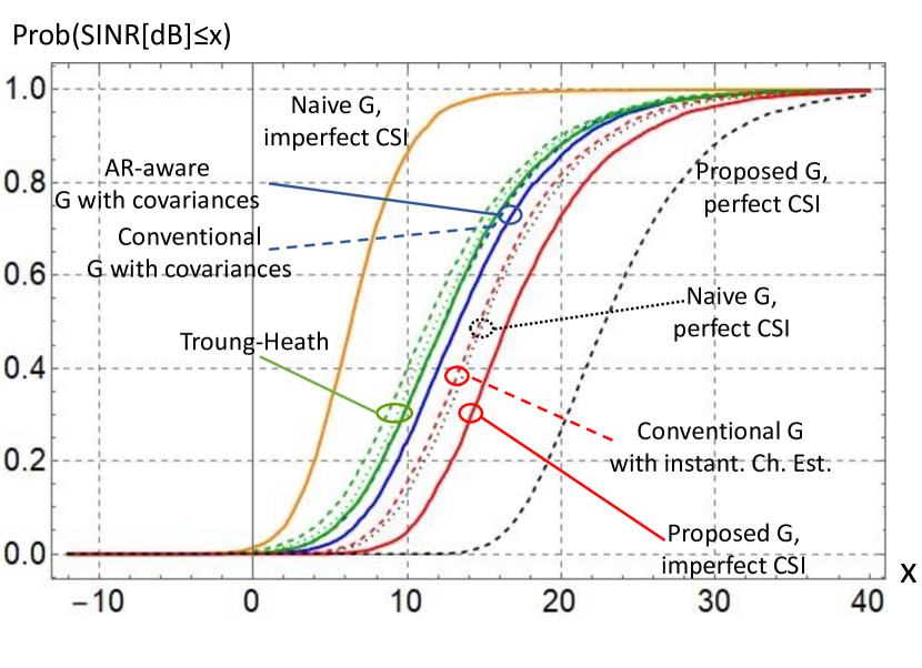
Figure 1: CDFs of the instantaneous SINR defined in (33) when using the proposed AR-aware MMSE receiver (red solid line) and previously proposed MU-MIMO receivers (see Table IV). Note the significant gain as compared with the AR-aware MU-MIMO receiver that treats interference as noise proposed in [13] and with Troung and Heath (1), (2), (3) proposed in [7].

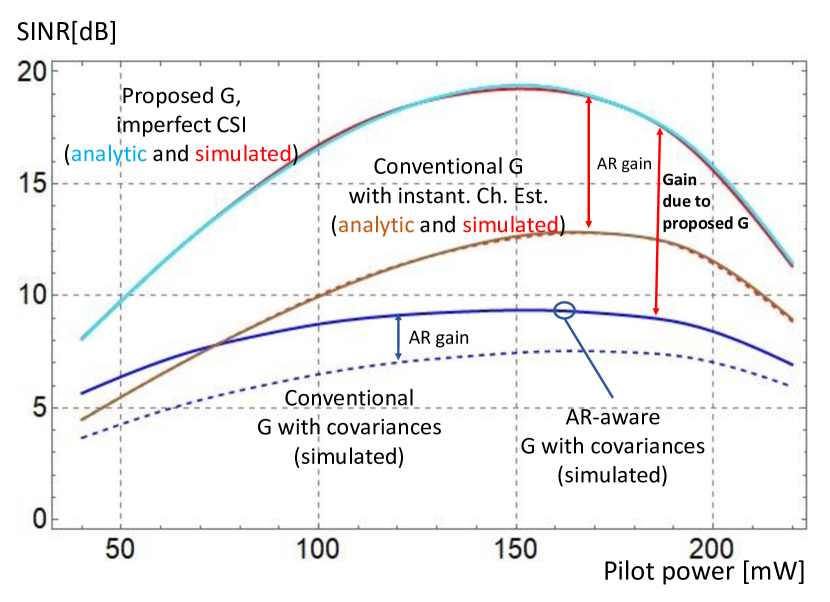
Figure 2: Average SINR as a function of the employed pilot power when using the proposed and the state of the art receivers. The SINR of the proposed receiver is both calculated using Theorem 2 and simulated. Similarly to the previous figure, we can see the significant gain of the proposed receiver over the receivers developed in [13] and [23].

Figure 1 shows the CDF of the SINR of the tagged user for the specific case when the number of users is $K=5$, number of receive antennas at the BS is $N_{r}=100$ and the pilot power is kept fixed at $P_{p}=100$ mW. Notice that the proposed receiver, which uses Kalman filter-assisted channel estimation for all users outperforms the conventional receiver, which does not use Kalman filter for channel estimation. The potential of the proposed MMSE receiver is indicated by the rightmost curve, which shows the SINR performance of this receiver if it has access to perfect channel estimates. Even in the presence of channel estimation errors, it outperforms all other receivers due to two reasons. First, its structure is modified as compared with previously proposed receivers and second, it takes advantage of the instantaneous channel estimates based on multiple observations (i.e. $\mathbf{\hat{h}}(t)$ and $\mathbf{\hat{h}}(t-1)$).

Figure 2 shows the average SINR performance of the proposed receiver, using Theorem 2, verified by simulations. The performance of the proposed receiver is compared both with that of the conventional receiver [18, 23] (termed MMSE receiver in those papers), and that of the AR-aware receiver proposed in [13], which uses the covariance matrices of the interfering users to suppress MU-MIMO interference. In this Figure, we refer to the gain over the first type of receivers as the "AR gain", since this gain is due to modified receiver structure, which makes it "AR aware". The gain over the receiver proposed in [13] is due to estimating all users’ channels, rather than treating the MU-MIMO interference as noise. This figure also shows that the analytical SINR calculation based on Theorem 2 gives a tight approximation.

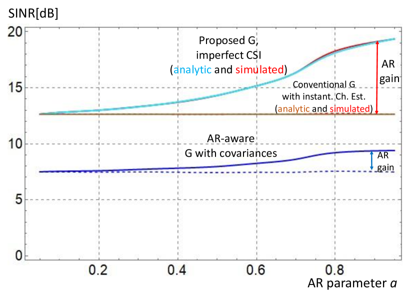
Figure 3: Average SINR as a function of the AR parameter $a$. The proposed receiver falls back to the receiver that is not AR-aware and uses the instantaneous channel estimates of all users [23] when $a$ is close to zero. Likewise, the receiver that uses the covariance matrices of the estimated channels [13] falls back to the conventional receiver [33] when $a=0$.

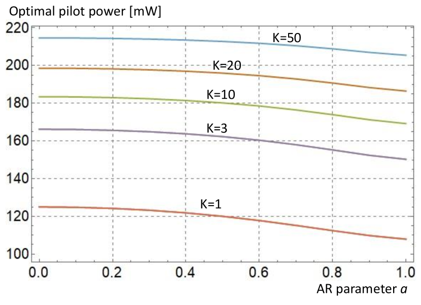
Figure 4: Optimum pilot power vs $a$ for $K=1,3,10,20,50$ users. Note that the optimum pilot power does not depend on the number of antennas. The optimal pilot power increases with increasing number of users when assuming a total pilot+data power budget.

Figure 3 compares the performance of AR-aware receiver developed in [13] with that of the proposed receiver in this current paper, as a function of the AR parameter $a$. The horizontal lines correspond to the SINR performance of the conventional receivers that do not exploit the memoryful property of the channel, that is they assume that $a=0$. First, notice that both receivers take advantage of the AR process of the channel when $a$ is close to 1 ("AR gain"). Second, the currently proposed receiver gains much more by exploiting the channel AR process than the receiver proposed in [13], since this receiver estimates the channels of all users rather than treating the interfering users as unknown noise. The sum of these two gains is quite significant when comparing the SINR performance of the conventional MU-MIMO receiver by the proposed MU-MIMO receiver when the autocorrelation coefficients of the user channels are high. Such high autocorrelation property can be achieved in practice by proper pilot symbol allocation in the time domain.

Figure 4 shows the optimum pilot power setting as a function of the AR parameter $a$ for systems in which the number of users is $K=1,3,10,20,50$. This figure assumes that the users are placed along a circle around the serving base station, that is, all users have the same path loss and set their pilot/data power ratio identically. as mentioned the optimum pilot power is invariant under of the number of receive antennas ($N_{r}$) as long as $N_{r}\geq K$. This figure clearly indicates that when the number of users is large, each user should increase its pilot power, which implies decreasing their data power due to the sum pilot and data power constraint. The main reason for this is that while the pilot signals do not cause interference to each other (due to the assumption on pilot sequence orthogonality), increasing the number of users increases the MU-MIMO interference level on the received data signals. Therefore, the optimum pilot allocation in the many users case tends to reduce data power and increase the pilot power levels. Furthermore, Figure 4 indicates that the optimum pilot power is decreasing with parameter $a$. An intuitive explanation of this behaviour is that the strong correlation of the channel state in consecutive periods makes easier to acquire the CSI.

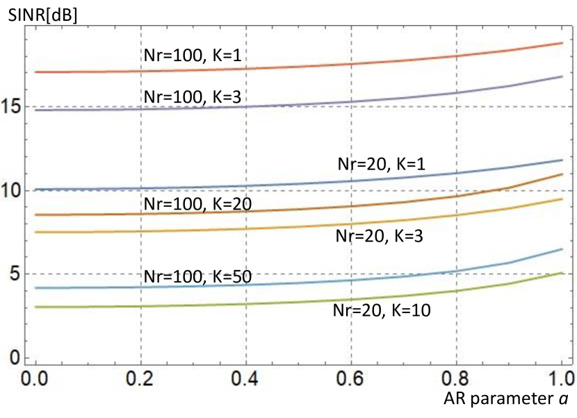
Figure 5: SINR when using the optimum pilot power vs $a$ for various number of users and antennas. The achieved SINR increases when the AR coefficient is high as compared with the case when the channel samples are uncorrelated (i.e. block fading) in time.

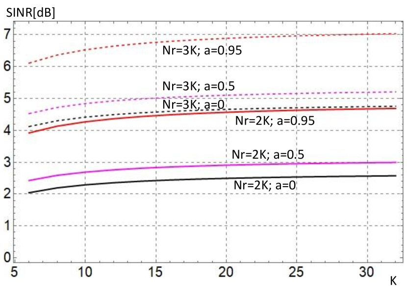
Figure 6: SINR vs K when $N_{r}=2K$ and when $N_{r}=3K$. The SINR performance of the $N_{r}=2K$ system with $a=0.95$ almost reaches that of the $N_{r}=3K$ system with $a=0$.

Figure 5 shows the achieved SINR when pilot power is set optimally, as a function of the AR coefficient $a$. Again, we notice that the performance increases as $a$ increases for all cases. Also, the SINR performance of a system with $N_{r}=100$ and $K=50$ users is somewhat higher than that of a system with $N_{r}=20$ and $K=10$. This is expected, since larger number of antennas implies an improved array gain for all users. We can also see that the gain due to increasing $a$ is similar in all cases.

Figure 6 uses Theorem 2 to calculate the average SINR as a function of the number of users $K$ when the number of antennas is set to $N_{r}=2K$ and $N_{r}=3K$ and when setting $a=0$, $a=0.5$ and $a=0.95$. Here we can see that setting $N_{r}=2K$ with $a=0.95$ gives almost the same SINR performance as when having $N_{r}=3K$ antennas with $a=0$. This result indicates that when the pilot symbols are sufficiently densely spaced and the autocorrelation in the channel is well exploited, much lower number of antennas can give a similar SINR performance as that of a system with a high number of antennas.

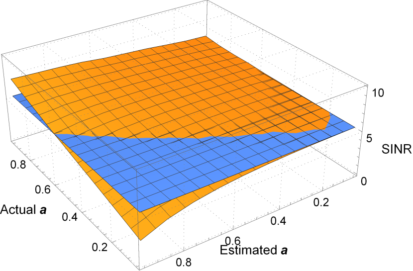
Figure 7: Average SINR vs the actual and the estimated AR parameters ($a$ and $\hat{a}$). The flat surface indicates the average SINR performance in a system where $a=0$, which is correctly assumed by the receiver.

Figure 7 illustrates the sensitivity of the achieved average SINR when using proposed receiver with respect to the difference between the estimated and actual $a$ parameters of the AR channel. The figure shows the actually achieved average SINR in a system with $N_{r}=20$ antennas and $K=5$ users, as a function of the actual ($a$) and estimated ($\hat{a}$) AR parameter. The flat surface indicates the SINR level that is achieved in a system with $a=0$ that correctly assumes that $a=0$.

When the actual $a$ is high (greater than 0.8), the achieved SINR is higher than when $a=0$, for all estimated $\hat{a}$ values. However, when the actual $a$ is low (the channel is effectively block fading) and the estimated $\hat{a}$ is high (the receiver assumes strong correlation in the subsequent channel estimates), the achieved SINR is lower than what is achieved by a conventional receiver. This result suggests that with proper pilot symbol spacing, when $a$ is high, estimating well the $a$ is also important to fully harvest the gains by using the proposed receiver.

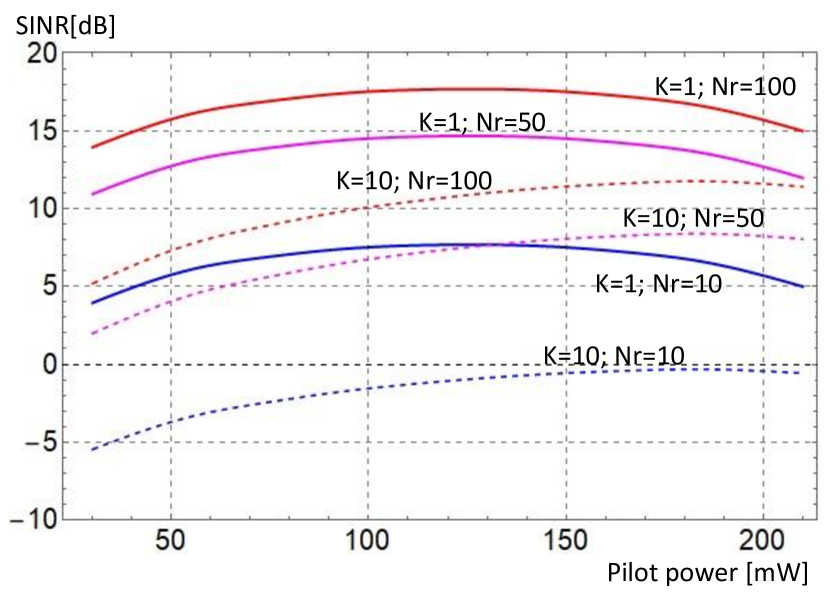
Figure 8: SINR performance calculated analytically using Theorem 2 of the proposed AR-aware $\mathbf{G}^{\star}$ receiver as a function of the pilot power in different scenarios in terms of number of users $K$ (i.e. single user or $K=10$) and number of antennas at the BS, (i.e. $N_{r}=10,50,100$) at $a=0$.

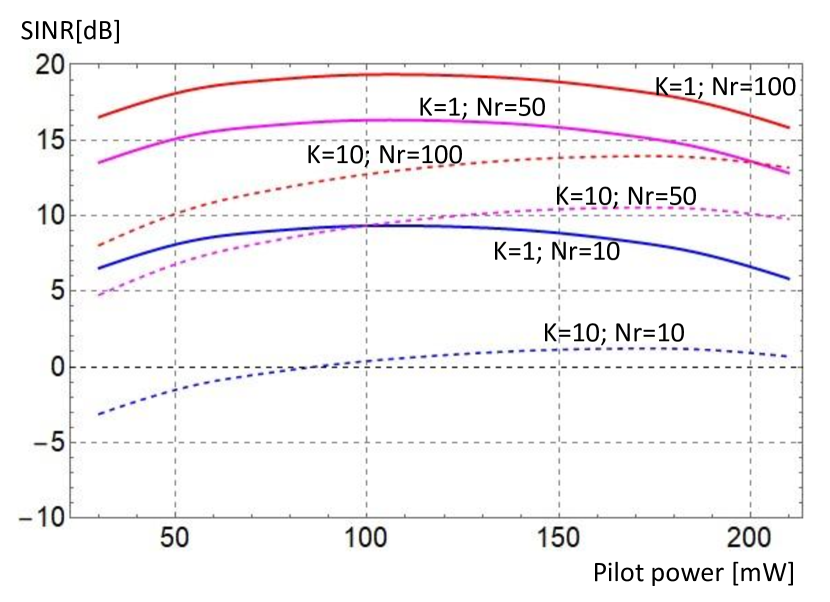
Figure 9: SINR performance calculated analytically using Theorem 2 of the proposed AR-aware $\mathbf{G}^{\star}$ receiver as a function of the pilot power in different scenarios in terms of number of users $K$ (i.e. single user or $K=10$) and number of antennas at the BS, (i.e. $N_{r}=10,50,100$) at $a=0.95$.

Finally, Figures 8 and 9 compare the average SINR performance of single and multiuser ($K=10$) systems when $a=0$ and when $a=0.95$ when the number of base station antennas is low $N_{r}=10$ and high $N_{r}=50$ or $N_{r}=100$. Notice that in the case of a memoryful MIMO channel ($a=0.95$) properly setting the pilot power and exploiting the memoryful property of the channel, an average SINR above 0 dB can be achieved even with a relatively low number of antennas (see the case of $N_{r}=K=10$), whereas in the case of $a=0$ the average SINR stays below 0 dB, especially if the pilot power is not properly tuned.

VI Conclusions and Outlook

In this paper we proposed a new MU-MIMO receiver, whose distinguishing features are its capability to utilize the instantaneous channel estimate of each user, and to exploit the memoryful property of the MU-MIMO wireless channels (AW-awareness) when these channels evolve according the an AR process. The main contribution of this paper is the new MU-MIMO receiver structure (Proposition 1) and its performance analysis facilitated by Proposition 2 and Theorem 2. This receiver and its performance analysis extends the results by [18] in the sense that (1) the proposed receiver exploits the memoryful property of the AR channels rather than treating them as block fading and (2) due to Theorem 2 it allows the calculate the average SINR without solving a system of fixed point equations. Our numerical results indicate that the proposed receiver outperforms previously proposed MU-MIMO receivers. An important future work, which is outside the scope of the present paper, is to find the optimal pilot power levels when the users are randomly placed in the coverage area of the cell, and, consequently, have different large scale fading parameters. Also, in the light of the results by multicell MU-MIMO receivers studied by [20], [21] and [22] in block fading environments, it is an exciting question, whether the proposed receiver in this paper can be extended to multicell systems.

Appendix A Proof of Lemma 1

Proof.

The MMSE channel estimator aims at minimizing the MSE between the channel estimate $\mathbf{\hat{h}}_{\textrm{MMSE}}(t)=\mathbf{H}^{\star}\mathbf{\hat{Y}}^{p}(t)$ and the channel $\mathbf{h}(t)$, where $\mathbf{H}\in\mathds{C}^{N_{r}\times 2\tau_{p}N_{r}}$, $\mathbf{\hat{Y}}^{p}(t)=\begin{bmatrix}\mathbf{\tilde{Y}}^{p}(t)\\ \mathbf{\tilde{Y}}^{p}(t-1)\end{bmatrix}\in\mathds{C}^{2\tau_{p}N_{r}\times 1}$ and $\mathbf{H^{\star}}=\text{arg}\min_{\mathbf{H}}\mathds{E}_{\mathbf{h},\mathbf{n}}\{||\mathbf{H}\mathbf{\hat{Y}}^{p}(t)-\mathbf{h}(t)||_{F}^{2}\}$. The solution of this quadratic optimization problem is $\mathbf{H^{\star}}=\mathbf{b}^{H}\mathbf{F}^{-1}$ with

$$\mathbf{F} =\mathds{E}_{\mathbf{h},\mathbf{n}}\left(\mathbf{\hat{Y}}^{p}\mbox{$\mathbf{\hat{Y}}^{p}$}^{H}\right)$$

$$=\begin{bmatrix}\alpha^{2}P_{p}\mathbf{S}\mathbf{C}\mathbf{S}^{H}+\sigma_{p}^{2}\mathbf{I}_{N_{r}\tau_{p}}&\alpha^{2}P_{p}\mathbf{S}(\mathbf{A}\mathbf{C})\mathbf{S}^{H}\\ \alpha^{2}P_{p}\mathbf{S}(\mathbf{C}\mathbf{A}^{H})\mathbf{S}^{H}&\alpha^{2}P_{p}\mathbf{S}\mathbf{C}\mathbf{S}^{H}+\sigma_{p}^{2}\mathbf{I}_{N_{r}\tau_{p}}\end{bmatrix}$$

$$=\alpha^{2}P_{p}\leavevmode\nobreak\ \left(\mathbf{s}\mathbf{s}^{H}\otimes\mathbf{M}\right)+\sigma_{p}^{2}\mathbf{I}_{2N_{r}\tau_{p}},$$

$$\mathbf{b} =\mathds{E}_{\mathbf{h},\mathbf{n}}\left(\mathbf{\hat{Y}}^{p}\mathbf{h}^{H}(t)\right)=\begin{bmatrix}\alpha\sqrt{P_{p}}\mathbf{S}\mathbf{C}\\ \alpha\sqrt{P_{p}}\mathbf{S}(\mathbf{C}\mathbf{A}^{H})\end{bmatrix}$$

$$=\alpha\sqrt{P_{p}}\leavevmode\nobreak\ \leavevmode\nobreak\ \left(\mathbf{s}\otimes\begin{bmatrix}\mathbf{C}\\ \mathbf{C}\mathbf{A}^{H}\end{bmatrix}\right),$$

where we utilized $\mathbf{S}\triangleq\mathbf{s}\otimes\mathbf{I}_{N_{r}}$ and $\mathbf{S}^{H}\mathbf{\tilde{N}}(t)=\mathbf{s}^{H}\mathbf{N}(t)$. That is

$$\mathbf{H^{\star}} =\mathbf{b}^{H}\mathbf{F}^{-1}$$

$$=\frac{1}{\alpha\sqrt{P_{p}}\tau_{p}}\begin{bmatrix}\mathbf{C}&\mathbf{A}\mathbf{C}\end{bmatrix}\left(\frac{\sigma_{p}^{2}}{\alpha^{2}P_{p}\tau_{p}}\mathbf{I}_{2N_{r}}+\mathbf{M}\right)^{-1}\left(\mathbf{s}^{H}\otimes\mathbf{I}\right).$$

The MMSE estimate is then expressed as

$$\mathbf{\hat{h}}_{\textrm{MMSE}}(t)=\mathbf{H^{\star}}\mathbf{\hat{Y}}^{p}(t)=\begin{bmatrix}\mathbf{C}&\mathbf{A}\mathbf{C}\end{bmatrix}\left(\frac{\sigma_{p}^{2}}{\alpha^{2}P_{p}\tau_{p}}\mathbf{I}_{2N_{r}}+\mathbf{M}\right)^{-1}$$

$$\leavevmode\nobreak\ \leavevmode\nobreak\ \leavevmode\nobreak\ \leavevmode\nobreak\ \leavevmode\nobreak\ \leavevmode\nobreak\ \leavevmode\nobreak\ \leavevmode\nobreak\ \leavevmode\nobreak\ \leavevmode\nobreak\ \leavevmode\nobreak\ \leavevmode\nobreak\ \leavevmode\nobreak\ \leavevmode\nobreak\ .\begin{bmatrix}\mathbf{h}(t)+\frac{1}{\alpha\sqrt{P_{p}}\tau_{p}}\mathbf{s}^{H}\mathbf{N}(t)\\ \mathbf{h}(t\!-\!1)+\frac{1}{\alpha\sqrt{P_{p}}\tau_{p}}\mathbf{s}^{H}\mathbf{N}(t\!-\!1)\end{bmatrix},$$ (63)

which gives the lemma. ∎

Appendix B Proof or Proposition 2

Starting from (41), we first apply [7, Lemma 1, eq. (47)] which states that, if $\left(\mathbf{B}\mathbf{B}^{H}+\bm{\beta}\right)^{-1}$ has a uniformly bounded spectral norm, then

$$\frac{1}{N_{r}}\mathbf{b}^{H}\left(\mathbf{B}\mathbf{B}^{H}+\bm{\beta}\right)^{-1}\mathbf{b}-\frac{1}{N_{r}}\text{tr}\left(\mathbf{\Phi}\left(\mathbf{B}\mathbf{B}^{H}+\bm{\beta}\right)^{-1}\right)\xrightarrow[N_{r}\rightarrow\infty]{\text{a.s.}}0.$$ (64)

In the second step we apply [18, Theorem 1], which states that, if $N_{r}\to\infty$ and $\limsup_{N_{r}\to\infty}K/N_{r}<\infty$, then

$$\frac{1}{N_{r}}\text{tr}\left(\mathbf{\Phi}\left(\mathbf{B}\mathbf{B}^{H}+\bm{\beta}\right)^{-1}\right)-\frac{1}{N_{r}}\text{tr}\Big{(}\mathbf{\Phi}\mathbf{T}\Big{)}\xrightarrow[N_{r}\rightarrow\infty]{\text{a.s.}}0,$$

$$\text{\leavevmode\nobreak\ where\leavevmode\nobreak\ \leavevmode\nobreak\ }\leavevmode\nobreak\ \mathbf{T}\triangleq\left(\frac{1}{N_{r}}\sum_{k=2}^{K}\frac{\mathbf{\Phi}_{k}}{1+\delta_{k}}+\bm{\beta}\right)^{-1},$$ (65)

and $\delta_{k}$, for $k=2,\ldots,K$ are the solution of

$$\delta_{k} =\frac{1}{N_{r}}\text{tr}\left(\mathbf{\Phi}_{k}\left(\frac{1}{N_{r}}\sum_{\ell=2}^{K}\frac{\mathbf{\Phi}_{\ell}}{1+\delta_{\ell}}+\bm{\beta}\right)^{-1}\right).$$ (66)

Adding equations (B) and (66) we get that

$$\mathbf{b}^{H}\left(\mathbf{B}\mathbf{B}^{H}+\bm{\beta}\right)^{-1}\mathbf{b}-\frac{1}{N_{r}}\text{tr}\Big{(}\mathbf{\Phi}\mathbf{T}\Big{)}\xrightarrow[N_{r}\rightarrow\infty]{\text{a.s.}}0,$$ (67)

which together with equation (41) gives the desired result.

Appendix C Proof of Theorem 1

To prove Theorem 1, we need the following Lemma regarding the moments of the random variable $\omega_{n}$:

Lemma 5.

Let $\omega_{n}$ and $\bar{\lambda}$ be defined as in Theorem 1, we can then state the following relationship between the moments of $\omega_{n}$ and the powers of $\bar{\lambda}$,

$$\lim_{n\rightarrow\infty}\frac{\mathds{E}\{\omega_{n}^{r}\}}{n^{r-1}}=\bar{\lambda}^{r}.$$ (68)

Proof of Lemma 5.

The random matrix $\mathbf{v}^{(n)}\left(\mathbf{v}^{(n)}\right)^{H}$ is rank one and thus has $n-1$ eigenvalues equal to 0 and one eigenvalue equal to $\text{tr}\left(\mathbf{v}^{(n)}\left(\mathbf{v}^{(n)}\right)^{H}\right)=\sum_{i=1}^{n}\|v^{(n)}_{i}\|^{2}$. Note that $Y_{i}\triangleq\|v^{(n)}_{i}\|^{2}$ has an exponential distribution with mean $\lambda_{i}$. Since $\omega_{n}$ is one of these eigenvalues, randomly selected, we have

$$\lim_{n\rightarrow\infty}\frac{\mathds{E}\{\omega_{n}^{r}\}}{n^{r-1}} =\lim_{n\rightarrow\infty}\frac{\frac{1}{n}\mathds{E}\{\left(\sum_{i=1}^{n}Y_{i}\right)^{r}\}}{n^{r-1}}$$

$$=\lim_{n\rightarrow\infty}\mathds{E}\left\{\left(\frac{\sum_{i=1}^{n}Y_{i}}{n}\right)^{r}\right\}.$$ (69)

Furthermore by the strong law of large numbers as $n\to\infty$

$$\frac{\sum_{i=1}^{n}Y_{i}}{n}\xrightarrow[n\rightarrow\infty]{\text{a.s.}}\bar{\lambda} \Rightarrow\left(\frac{\sum_{i=1}^{n}Y_{i}}{n}\right)^{r}\xrightarrow[n\rightarrow\infty]{\text{a.s.}}\bar{\lambda}^{r}$$

$$\Rightarrow\lim_{n\rightarrow\infty}\mathds{E}\left\{\left(\frac{\sum_{i=1}^{n}Y_{i}}{n}\right)^{r}\right\}=\bar{\lambda}^{r}.$$ (70)

Equations (69) and (C) give the Lemma. ∎

For the proof of the Theorem 1, in addition to Lemma 5, we will use the equivalent (cf. (54)) definition of the $\mathcal{R}$-transform of a random variable $X$ using its cumulants [37]:

$$\mathcal{R}_{X}(s)\triangleq\sum_{k=0}^{\infty}\kappa_{k+1}s^{k},$$ (71)

where $\kappa_{k}$ is the k’th cumulant of $X$, that is

$$\kappa_{k}=\left.\frac{d^{k}}{ds^{k}}K_{X}(s)\right|_{s=0}=K_{X}^{(k)}(0),$$ (72)

and $K_{X}(s)$ is the cumulant generating function $K_{X}(s)\triangleq\operatorname{\log}\mathds{E}\left[e^{sX}\right]$. We use this definition in the proof as it is often useful to have two equivalent definitions of a function, and use one of them to say something about the other. In this case we use the cumulant definition of the $\mathcal{R}$-transform to be able to state results about the Stieltjes transform. In order to calculate the cumulants $\kappa_{k}$ we calculate the value of the derivatives of $K_{X}(s)$ at $s=0$, we do this through the derivatives of the moment generating function $M_{X}(s)\triangleq\mathds{E}\left[e^{sX}\right]$ of $X$ as follows. First define $m_{i}(s)\triangleq M_{X}^{(i)}(s)/M_{X}(s)$, and define the order of the product

$$\prod_{k=1}^{K}m_{i_{k}}^{j_{k}}(s)\leavevmode\nobreak\ \leavevmode\nobreak\ \leavevmode\nobreak\ \text{to be}\leavevmode\nobreak\ \leavevmode\nobreak\ \leavevmode\nobreak\ \sum_{k=1}^{K}i_{k}j_{k}.$$ (73)

Notice that by the quotient rule

$$\frac{d}{ds}m_{i}(s) =\frac{d}{ds}\frac{M_{X}^{(i)}(s)}{M_{X}(s)}$$

$$=\frac{M_{X}^{(i+1)}(s)M_{X}(s)-M_{X}^{(i)}(s)M_{X}^{\prime}(s)}{M_{X}^{2}(s)}$$

$$=m_{i+1}(s)-m_{i}(s)m_{1}(s).$$ (74)

Thus, by the product rule the derivative of an order $k$ product is a sum of order $k+1$ products, and so the $k$’th cumulant

$$\kappa_{k} =\left.\frac{d^{k}}{ds^{k}}K_{X}(s)\right|_{s=0}=\left.\frac{d^{k-1}}{ds^{k-1}}m_{1}(s)\right|_{s=0},$$ (75)

is a sum of order $k$ products at $s=0$, and one of the terms of this sum is $m_{k}(0)$. Furthermore, by the definition of $m_{k}$, we have $m_{k}(0)=\mathds{E}\{X^{k}\}$.

More specifically, looking at the random variable $\omega_{n}$, we know from Lemma 5 that $\mathds{E}\{\omega_{n}^{k}\}$ and hence $m_{k}(0)$ is $O(n^{k-1})$. Consequently, any order $k$ product at $s=0$ other than $m_{k}(0)$ is $O(n^{k-2})$, and so by Lemma 5:

$$\lim_{n\rightarrow\infty}\frac{\kappa_{k}}{n^{k-1}} =\bar{\lambda}^{k}.$$ (76)

We can now derive (56):

$$\lim_{n\rightarrow\infty} \mathcal{R}_{\omega_{n}}\left(\frac{s}{n}\right)=\lim_{n\rightarrow\infty}\sum_{k=0}^{\infty}\kappa_{k+1}\left(\frac{s}{n}\right)^{k}$$

$$=\lim_{n\rightarrow\infty}\sum_{k=0}^{\infty}\frac{\kappa_{k+1}}{n^{k}}s^{k}=\sum_{k=0}^{\infty}\bar{\lambda}^{k+1}s^{k}=\frac{\bar{\lambda}}{1-s\bar{\lambda}},$$ (77)

which completes the proof.

Appendix D Proof of Theorem 2 Using the Stieltjes and $\mathcal{R}$-Transforms

The first proof of Theorem 2 relies on random matrix theory using the Stieltjes transform, the $\mathcal{R}$-transform and Corollary 2 of Theorem 1. To determine (52), we use the spectral decomposition of the Hermitian matrix and define $\mathbf{y}\triangleq\mathbf{U}\mathbf{b}$. Accordingly, (52) becomes

$$\bar{\gamma} =\mathds{E}_{\mathbf{y},\lambda_{i},i=1\ldots N_{r}}\left\{\mathbf{y}^{H}\mathbf{U}\mathbf{U}^{H}(\mathbf{\Lambda}+\beta\mathbf{I}_{N_{r}})^{-1}\mathbf{U}\mathbf{U}^{H}\mathbf{y}\right\}$$

$$=\mathds{E}_{\mathbf{y},\lambda_{i},i=1\ldots N_{r}}\left\{\sum_{i=1}^{N_{r}}\frac{|y_{i}|^{2}}{\lambda_{i}+\beta}\right\},$$

where $y_{i}$ is $i$th element of the vector $\mathbf{y}$ and $\lambda_{i}$ is the $i$th eigenvalue of $\mathbf{B}\mathbf{B}^{H}$.

Since the $\mathbf{U}$ matrix is unitary, $\mathbf{y}$ and $\mathbf{b}$, have same distribution, i.e. $\mathbf{y}\sim\mathcal{CN}(0,\phi\mathbf{I}_{N_{r}})$ and $\mathds{E}\left\{|y_{i}|^{2}\right\}=\phi;\leavevmode\nobreak\ i=1\dots N_{r}$, where recall that $\phi=\phi_{1}$ (tagged user). Moreover, since the interference matrix $\mathbf{B}\mathbf{B}^{H}$ is independent of $\mathbf{b}$, $\mathbf{y}$ is independent of the eigenvalues $\lambda_{i}$, and hence

$$\bar{\gamma}=\phi\cdot\mathds{E}_{\lambda_{i},i=1\ldots N_{r}}\left(\sum_{i=1}^{N_{r}}\frac{1}{\lambda_{i}+\beta}\right).$$ (78)

Assuming that $N_{r},K\rightarrow\infty$, with $K/N_{r}$ fixed, and using equations (13) and (14) of [43] we obtain:

$$\mathds{E}_{\lambda_{i},i=1\ldots N_{r}}\left\{\sum_{i=1}^{N_{r}}\frac{1}{\lambda_{i}+\beta}\right\} =N_{r}\mathds{E}_{\lambda}\left\{\frac{1}{\lambda+\beta}\right\},$$ (79)

where $\lambda$ is a randomly selected eigenvalue out of the spectrum of $\mathbf{B}\mathbf{B}^{H}$.

A first key observation is that the Stieltjes transform of the distribution of $\lambda$ at $s=-\beta$ is closely related to $\bar{\gamma}$:

$$G_{{\color[rgb]{0,0,0}{\lambda}}}(-\beta) \overset{(a)}{=}\int_{x}\frac{1}{x+\beta}dP_{\lambda}(x)\overset{(b)}{=}\mathds{E}_{\lambda}\left\{\frac{1}{\lambda+\beta}\right\}\overset{(c)}{=}\frac{\bar{\gamma}}{N_{r}\phi},$$ (80)

where $(a)$ is due to definition of the Stieltjes transform, and $(b)$ is due to noticing that the left hand side of $(b)$ is by definition the expectation of $1/(\lambda+\beta)$. Finally, in the last equation we used (78). This implies that if we can find an appropriate $\beta$ for which it holds that:

$$G_{\lambda}\left(-\beta\right)=w,$$ (81)

where $w\triangleq\frac{\bar{\gamma}}{N_{r}\phi}$, then according to (80) we found $\bar{\gamma}$ in the form of: $N_{r}\phi G_{\lambda}\left(-\beta\right)=\bar{\gamma}$. To find such a $\beta$, recall that for the Hermitian matrix associated with the tagged user $\mathbf{B}\mathbf{B}^{H}=\sum_{k=2}^{K}\mathbf{b}_{k}\mathbf{b}_{k}^{H}$ with

$$\mathbf{b}_{k} \sim\mathcal{CN}(0,\phi_{k}\mathbf{I}_{N_{r}}).$$ (82)

Furthermore, we will utilize the following identity (see (54)):

$$G_{\lambda}\left(\mathcal{R}_{\lambda}(-w)-\frac{1}{w}\right) =w.$$ (83)

Furthermore, assuming that $N_{r}\rightarrow\infty$, the family of matrices $\mathbf{b}_{k}\mathbf{b}_{k}^{H}$ ($k=1,\dots,K$) is almost surely asymptotically free [37]. Consequently, the $\mathcal{R}$-transform of the sum of matrices $\mathbf{b}_{k}\mathbf{b}_{k}^{H}$ equals the sum of their individual $\mathcal{R}$-transforms.

Recall that by Corollary 2, the $\mathcal{R}$-transform of a randomly selected eigenvalue $\omega$ of $\mathbf{b}_{k}\mathbf{b}_{k}^{H}$ is ${\color[rgb]{0,0,0}{R_{\omega}(w)}}\approx\frac{\phi_{k}}{1-N_{r}\phi_{k}w}$. Hence, utilizing the additive property of the $\mathcal{R}$-transform, for a randomly selected eigenvalue $\Omega$ of $\mathbf{B}\mathbf{B}^{H}$ we get:

$${\color[rgb]{0,0,0}{\mathcal{R}_{\Omega}(w)}} =\sum_{k=2}^{K}\frac{\phi_{k}}{1-N_{r}\phi_{k}w}.$$ (84)

Substituting (84) into (83) we have:

$$G\left(\sum_{k=2}^{K}\frac{\phi_{k}}{1{\color[rgb]{0,0,0}{+}}N_{r}\phi_{k}w}-\frac{1}{w}\right)=w,$$ (85)

for all $w>0$. From this equation it is also evident that the expression inside the $G$-transform is injective for $w>0$. Comparing (81) and (83), we have that:

$$-\beta =\mathcal{R}_{\lambda}(-w)-\frac{1}{w}$$ (86)

with $w=\frac{\bar{\gamma}}{N_{r}\phi}$, from which, using (85), it follows that $\bar{\gamma}$ satisfies the equation:

$$\beta =\left.\frac{1}{w}-\sum_{k=2}^{K}\frac{\phi_{k}}{1+N_{r}\phi_{k}w}\right|_{w=\frac{\bar{\gamma}}{N_{r}\phi}},$$ (87)

which is equivalent with (58). It is important to note that there cannot be more than one value of $\bar{\gamma}$ that satisfies the equation above since the RHS is injective in $w$.

Appendix E Proof or Theorem 2 Using the Trace Approximation

To prove Theorem 2, we first notice that in the special case of diagonal covariances with equal elements, we have that (see (50)):

$$\bm{\Phi} =\phi\mathbf{I}_{N_{r}}=\alpha^{2}P\left(\hat{e}c+\check{e}ca^{*}\right)\mathbf{I}_{N_{r}}.$$ (88)

In this special case, i.e. when $\bm{\Phi}$ is diagonal with equal diagonal elements, from (45) it follows that for the tagged user (User-$1$), it holds that:

$$\bar{\gamma} \approx\phi\cdot\text{tr}\left(\mathbf{T}\right).$$ (89)

Also, in this case, the definition of $\mathbf{T}$ in (43) simplifies to:

$$\mathbf{T} \triangleq\bigg{(}\frac{1}{N_{r}}\sum_{j=2}^{K}\frac{\phi_{j}}{1+\delta_{j}}\mathbf{I}_{N_{r}}+\underbrace{\sum_{k=1}^{K}\alpha_{k}^{2}P_{k}z_{k}\mathbf{I}_{N_{r}}+\sigma_{d}^{2}\mathbf{I}_{N_{r}}}_{\triangleq\beta\mathbf{I}_{N_{r}}}\bigg{)}^{-1},$$ (90)

where, according to [18] and [34], the $\delta_{j}$:s satisfy:

$$\delta_{k} =\phi_{k}\cdot\text{tr}\left(\left(\frac{1}{N_{r}}\sum_{j=2}^{K}\frac{\phi_{j}}{1+\delta_{j}}+\beta\right)^{-1}\mathbf{I}_{N_{r}}\right);\leavevmode\nobreak\ \leavevmode\nobreak\ k=2\dots K.$$ (91)

Comparing (89), (90) and (91), we notice that: $\delta_{k}=\phi_{k}\cdot\frac{\bar{\gamma}}{\phi}\leavevmode\nobreak\ \forall k\neq 1$. Substituting this into (91), we obtain:

$$\bar{\gamma} =N_{r}\phi\left(\sum_{j=2}^{K}\frac{\phi_{j}}{1+\frac{\phi_{j}}{\phi}\bar{\gamma}}+\beta\right)^{-1}.$$ (92)

From this equation we get $\beta=\frac{N_{r}\phi}{\bar{\gamma}}-\sum_{j=2}^{K}\frac{\phi_{j}}{1+\frac{\phi_{j}}{\phi}\bar{\gamma}},$ which is identical with (58).

Appendix F Proof of Proposition 3

Proof.

First notice that substituting $\phi=\alpha^{2}P(\hat{e}c+\check{e}ca)$, $\beta=K\alpha^{2}z+\sigma_{d}^{2}$, and $z=c-(\hat{e}c+\check{e}ca)$, the optimization problem in (60) can be rewritten as:

$$\underset{P,P_{p}}{\text{minimize}} \frac{Kc+\frac{\sigma_{d}^{2}}{\alpha^{2}P}}{\hat{e}c+\check{e}ca}-K\leavevmode\nobreak\ \leavevmode\nobreak\ \leavevmode\nobreak\ \leavevmode\nobreak\ \text{subject to}\leavevmode\nobreak\ \leavevmode\nobreak\ P\tau_{d}+P_{p}\tau_{p}=P_{\text{tot}}.$$ (93)

By substituting $P=(P_{\textup{tot}}-P_{p}\tau_{p})/\tau_{d}$, the values of $\hat{e}$ and $\check{e}$ from (IV-C) into the objective function, the optimization task in (93) is further equivalent with:

$$\underset{P_{p}}{\text{minimize}} \frac{\left(Kc+\frac{\sigma_{d}^{2}\tau_{d}}{\alpha^{2}(P_{\textup{tot}}-P_{p}\tau_{p})}\right)\left(\left(c+\frac{\sigma_{p}^{2}}{\alpha^{2}P_{p}\tau_{p}}\right)^{2}+a^{2}c^{2}\right)}{(a^{2}+1)\frac{\sigma_{p}^{2}}{\alpha^{2}P_{p}\tau_{p}}+c-a^{2}c}.$$ (94)

Notice that this expression approaches infinity both when $P_{p}\rightarrow 0$ and when $P_{p}\rightarrow P_{\textup{tot}}/\tau_{p}$:

$$\lim_{P_{p}\rightarrow 0}\frac{\left(Kc+\frac{\sigma_{d}^{2}\tau_{d}}{\alpha^{2}(P_{\textup{tot}}-P_{p}\tau_{p})}\right)\left(\left(c+\frac{\sigma_{p}^{2}}{\alpha^{2}P_{p}\tau_{p}}\right)^{2}+a^{2}c^{2}\right)}{(a^{2}+1)\frac{\sigma_{p}^{2}}{\alpha^{2}P_{p}\tau_{p}}+c-a^{2}c}$$

$$=\left(Kc+\frac{\sigma_{d}^{2}\tau_{d}}{\alpha^{2}P_{\textup{tot}}}\right)\lim_{P_{p}\rightarrow 0}\frac{\left(c+\frac{\sigma_{p}^{2}}{\alpha^{2}P_{p}\tau_{p}}\right)^{2}+a^{2}c^{2}}{(a^{2}+1)\frac{\sigma_{p}^{2}}{\alpha^{2}P_{p}\tau_{p}}+c-a^{2}c}\times\frac{P_{p}}{P_{p}}$$

$$=\left(Kc+\frac{\sigma_{d}^{2}\tau_{d}}{\alpha^{2}P_{\textup{tot}}}\right)\frac{\lim\limits_{P_{p}\rightarrow 0}P_{p}\left(c+\frac{\sigma_{p}^{2}}{\alpha^{2}P_{p}\tau_{p}}\right)^{2}}{(a^{2}+1)\frac{\sigma_{p}^{2}}{\alpha^{2}\tau_{p}}}=\infty;$$ (95)

$$\lim_{P_{p}\rightarrow P_{\textup{tot}}/\tau_{p}}\frac{\left(Kc+\frac{\sigma_{d}^{2}\tau_{d}}{\alpha^{2}(P_{\textup{tot}}-P_{p}\tau_{p})}\right)\left(\left(c+\frac{\sigma_{p}^{2}}{\alpha^{2}P_{p}\tau_{p}}\right)^{2}+a^{2}c^{2}\right)}{(a^{2}+1)\frac{\sigma_{p}^{2}}{\alpha^{2}P_{p}\tau_{p}}+c-a^{2}c}$$

$$=\frac{\left(c+\frac{\sigma_{p}^{2}}{\alpha^{2}P_{\textup{tot}}}\right)^{2}+a^{2}c^{2}}{(a^{2}+1)\frac{\sigma_{p}^{2}}{\alpha^{2}P_{\textup{tot}}}+c-a^{2}c}\lim_{P_{p}\rightarrow P_{\textup{tot}}/\tau_{p}}\left(Kc+\frac{\sigma_{d}^{2}\tau_{d}}{\alpha^{2}(P_{\textup{tot}}-P_{p}\tau_{p})}\right)$$

$$\leavevmode\nobreak\ \leavevmode\nobreak\ \leavevmode\nobreak\ =\infty.$$ (96)

Since the expression to minimize is positive over the interval $\left(0,P_{\textup{tot}}/\tau_{p}\right)$, and approaches infinity at the edges of the interval, there is a global minimum in the interval which is also a stationary point. To find the set of all stationary points, we calculate the derivative of the expression in equation (94) with respect to $P_{p}$. We have:

$$\frac{d}{dP_{p}}\left(Kc+\frac{\sigma_{d}^{2}\tau_{d}}{\alpha^{2}(P_{\textup{tot}}-P_{p}\tau_{p})}\right)=\frac{\sigma_{d}^{2}\tau_{d}}{\alpha^{2}(P_{\textup{tot}}-P_{p}\tau_{p})^{2}}$$

$$\frac{d}{dP_{p}}\left(\left(c+\frac{\sigma_{p}^{2}}{\alpha^{2}P_{p}\tau_{p}}\right)^{2}+a^{2}c^{2}\right)=$$

$$\leavevmode\nobreak\ \leavevmode\nobreak\ \leavevmode\nobreak\ \leavevmode\nobreak\ \leavevmode\nobreak\ \leavevmode\nobreak\ \leavevmode\nobreak\ \leavevmode\nobreak\ \leavevmode\nobreak\ \leavevmode\nobreak\ \leavevmode\nobreak\ \leavevmode\nobreak\ \leavevmode\nobreak\ \leavevmode\nobreak\ \leavevmode\nobreak\ \leavevmode\nobreak\ \leavevmode\nobreak\ \leavevmode\nobreak\ \leavevmode\nobreak\ \leavevmode\nobreak\ \leavevmode\nobreak\ \leavevmode\nobreak\ \leavevmode\nobreak\ \leavevmode\nobreak\ \leavevmode\nobreak\ \leavevmode\nobreak\ \leavevmode\nobreak\ \leavevmode\nobreak\ \leavevmode\nobreak\ \leavevmode\nobreak\ =-2\left(c+\frac{\sigma_{p}^{2}}{\alpha^{2}P_{p}\tau_{p}}\right)\frac{\sigma_{p}^{2}}{\alpha^{2}P_{p}^{2}\tau_{p}}$$

$$\frac{d}{dP_{p}}\left((a^{2}+1)\frac{\sigma_{p}^{2}}{\alpha^{2}P_{p}\tau_{p}}+c-a^{2}c\right)=-(a^{2}+1)\frac{\sigma_{p}^{2}}{\alpha^{2}P_{p}^{2}\tau_{p}}.$$ (97)

From this we can calculate the derivative of (94) with respect to $P_{p}$, which is a rational function with numerator equal to the polynomial given in equation (62), Hence, this polynomial has at least one positive root in the interval $\left(0,P_{\textup{tot}}/\tau_{p}\right)$, one of which gives the solution to the optimization task (94), and hence the optimal pilot power. ∎

References

- [1] M. Yan and D. Rao, “Performance of an array receiver with a Kalman channel predictor for fast Rayleigh flat fading environments,” IEEE Journal on Selected Areas in Communications, vol. 6, no. 6, pp. 1164–1172, 2001.
- [2] Y. Zhang, S. B. Gelfand, and M. P. Fitz, “Soft-output demodulation on frequency-selective rayleigh fading channels uing AR channel models,” IEEE Transactions on Communications, vol. 55, no. 10, pp. 1929–1939, Oct. 2007.
- [3] F. Lehmann, “Blind estimation and detection of space-time trellis coded transmissions over the rayleigh fading MIMO channel,” IEEE Transactions on Communications, vol. 56, no. 3, pp. 334–338, Mar. 2008.
- [4] H. Abeida, “Data-aided SNR estimation in time-variant rayleigh fading channels,” IEEE Transactions on Signal Processing, vol. 58, no. 11, pp. 5496–5507, Nov. 2010.
- [5] H. Hijazi and L. Ros, “Joint data QR-detection and Kalman estimation for OFDM time-varying rayleigh channel complex gains,” IEEE Transactions on Communications, vol. 58, no. 1, pp. 170–177, Jan. 2010.
- [6] S. Ghandour-Haidar, L. Ros, and J.-M. Brossier, “On the use if first-order autorgegressive modeling for rayleigh flat fading channel estimation with Kalman filter,” Elsevier Signal Processing, no. 92, pp. 601–606, 2012.
- [7] K. T. Truong and R. W. Heath, “Effects of channel aging in massive MIMO systems,” Journal of Communications and Networks, vol. 15, no. 4, pp. 338–351, 2013.
- [8] C. Kong, C. Zhong, A. K. Papazafeiropoulos, M. Matthaiou, and Z. Zhang, “Sum-rate and power scaling of massive MIMO systems with channel aging,” IEEE Transactions on Communications, vol. 63, no. 12, pp. 4879–4893, 2015.
- [9] L.-K. Chiu and S.-H. Wu, “An effective approach to evaluate the training and modeling efficacy in MIMO time-varying fading channels,” IEEE Transactions on Communications, vol. 63, no. 1, pp. 140–155, Jan. 2015.
- [10] S. Kashyap, C. Mollen, E. Björnson, and E. G. Larsson, “Performance analysis of (tdd) massive MIMO with Kalman channel prediction,” in IEEE International Conference on Acoustics, Speech and Signal Processing (ICASSP). New Orleans, LA, USA: IEEEE, Mar. 2017.
- [11] H. Kim, S. Kim, H. Lee, C. Jang, Y. Choi, and J. Choi, “Massive MIMO channel prediction: Kalman filtering vs. machine learning,” IEEE Transactions on Communications, pp. 1–1, 2020, early access.
- [12] J. Yuan, H. Q. Ngo, and M. Matthaiou, “Machine learning-based channel prediction in massive MIMO with channel aging,” IEEE Transactions on Wireless Communications, vol. 19, no. 5, pp. 2960–2973, 2020.
- [13] G. Fodor, S. Fodor, and M. Telek, “Performance analysis of a linear MMSE receiver in time-variant Rayleigh fading channels,” IEEE Transactions on Communications, vol. 69, no. 6, pp. 4098–4112, 2021.
- [14] R. Couillet, M. Debbah, and J. W. Silverstein, “A deterministic equivalent for the analysis of correlated MIMO multiple access channels,” IEEE Transactions on Information Theory, vol. 57, no. 6, pp. 3493–3514, 2011.
- [15] L. Hanlen and A. Grant, “Capacity analysis of correlated MIMO channels,” IEEE Transactions on Information Theory, vol. 58, no. 11, pp. 6773–6787, 2012.
- [16] R. Couillet, J. Hoydis, and M. Debbah, “Random beamforming over quasi-static and fading channels: A deterministic equivalent approach,” IEEE Transactions on Information Theory, vol. 58, no. 10, pp. 6392–6425, 2012.
- [17] C. Wen, G. Pan, K. Wong, M. Guo, and J. Chen, “A deterministic equivalent for the analysis of non-gaussian correlated MIMO multiple access channels,” IEEE Transactions on Information Theory, vol. 59, no. 1, pp. 329–352, 2013.
- [18] J. Hoydis, S. ten Brink, and M. Debbah, “Massive MIMO in the UL/DL of cellular networks: How many antennas do we need?” IEEE Journal on Selected Areas in Communications, vol. 31, no. 2, pp. 160–171, 2013.
- [19] A. Papazafeiropoulos and T. Ratnarajah, “Modeling and performance of uplink cache-enabled massive MIMO heterogeneous networks,” IEEE Transactions on Wireless Communications, vol. 17, no. 12, pp. 8136–8149, 2018.
- [20] E. Björnson, J. Hoydis, and L. Sanguinetti, “Massive MIMO has unlimited capacity,” IEEE Transactions on Wireless Communications, vol. 17, no. 1, pp. 574–590, Jan. 2018.
- [21] I. Boukhedimi, A. Kammoun, and M.-S. Alouini, “Line-of-Sight and pilot contamination effects on correlated multi-cell massive MIMO systems,” in 2018 IEEE Global Communications Conference (GLOBECOM), 2018, pp. 1–7.
- [22] L. Sanguinetti, E. Björnson, and A. Kammoun, “Large-system analysis of massive MIMO with optimal M-MMSE processing,” in 2019 IEEE 20th International Workshop on Signal Processing Advances in Wireless Communications (SPAWC), 2019, pp. 1–5.
- [23] A. Abrardo, G. Fodor, M. Moretti, and M. Telek, “MMSE receiver design and SINR calculation in MU-MIMO systems with imperfect CSI,” IEEE Wireless Communications Letters, vol. 8, no. 1, pp. 269–272, Feb. 2019.
- [24] R. Chopra and C. R. Murthy, “Data aided MSE-optimal time varying channel tracking in massive MIMO systems,” IEEE Transactions on Signal Processing, vol. 69, pp. 4219–4233, 2021.
- [25] A. Kammoun, A. Müller, E. Björnson, and M. Debbah, “Linear precoding based on polynomial expansion: Large-scale multi-cell MIMO systems,” IEEE Journal of Selected Topics in Signal Processing, vol. 8, no. 5, pp. 861–875, 2014.
- [26] A. Müller, R. Couillet, E. Björnson, S. Wagner, and M. Debbah, “Interference-aware RZF precoding for multicell downlink systems,” IEEE Transactions on Signal Processing, vol. 63, no. 15, pp. 3959–3973, 2015.
- [27] S. Sesia, I. Toufik, and M. Baker, LTE - The UMTS Long Term Evolution: From Theory to Practice. WILEY, 2nd edition, 2011, ISBN-10: 0470660252.
- [28] G. Fodor, P. D. Marco, and M. Telek, “Performance analysis of block and comb type channel estimation for massive MIMO systems,” in First International Conference on 5G, Akaslompolo, Finland, 2014.
- [29] H. Q. Ngo, M. Matthaiou, and E. G. Larsson, “Massive MIMO with optimal power and training duration allocation,” IEEE Wireless Communications Letters, vol. 3, no. 6, pp. 605–608, Dec. 2014.
- [30] M. McGuire and M. Sima, “Low-order Kalman filters for channel estimation,” in IEEE Pacific Rim Conference on Communications, Computers and Signal Processing (PACRIM), Victoria, BC, Canada, Aug. 2005, pp. 352–355.
- [31] Z. B. Krusevac and P. B. Rapajic, “Adaptive AR channel model identification of time-varying communication systems,” in IEEE 10th International Symposium on Spread Spectrum Techniques and Applications, Bologna, Italy, Aug. 2008.
- [32] S. Mekki, M. Amara, A. Feki, and S. Valentin, “Channel gain prediction for wireless links with Kalman filters and expectation-maximization,” in IEEE Wireless Communications and Networking Conference (WCNC), Doha, Qatar, Apr. 2016.
- [33] G. Fodor, P. D. Marco, and M. Telek, “On minimizing the MSE in the presence of channel information errors,” IEEE Communications Letters, vol. 19, no. 9, pp. 1604 – 1607, September 2015.
- [34] S. Wagner, R. Couillet, M. Debbah, and D. T. M. Slock, “Large system analysis of linear precoding in correlated MISO broadcast channels under limited feedback,” IEEE Transactions on Information Theory, vol. 58, no. 7, pp. 4509–4537, 2012.
- [35] R. Couillet, M. Debbah, and J. W. Silverstein, “A deterministic equivalent for the analysis of correlated MIMO multiple access channels,” IEEE Transactions on Information Theory, vol. 57, no. 6, pp. 3493–3514, 2011.
- [36] R. Couillet, J. Hoydis, and M. Debbah, “Random beamforming over quasi-static and fading channels: A deterministic equivalent approach,” IEEE Transactions on Information Theory, vol. 58, no. 10, pp. 6392–6425, 2012.
- [37] R. R. Müller, G. Alfano, B. M. Zaidel, and R. de Miguel, “Applications of large random matrices in communications engineering,” arXiV, vol. [cs.IT], no. 1310:5479, 2013.
- [38] C.-K. Wen, G. Pan, K.-K. Wong, M. Guo, and J.-C. Chen, “A deterministic equivalent for the analysis of non-gaussian correlated MIMO multiple access channels,” IEEE Transactions on Information Theory, vol. 59, no. 1, pp. 329–352, 2013.
- [39] J. Zhang, C.-K. Wen, S. Jin, X. Gao, and K.-K. Wong, “On capacity of large-scale MIMO multiple access channels with distributed sets of correlated antennas,” IEEE Journal on Selected Areas in Communications, vol. 31, no. 2, pp. 133–148, 2013.
- [40] A. Tulino, A. Lozano, and S. Verdu, “Impact of antenna correlation on the capacity of multiantenna channels,” IEEE Transactions on Information Theory, vol. 51, no. 7, pp. 2491–2509, 2005.
- [41] E. Eraslan, B. Daneshrad, and C.-Y. Lou, “Performance indicator for MIMO MMSE receivers in the presence of channel estimation error,” IEEE W. Comm. Letters, vol. 2, no. 2, pp. 211–214, April 2013.
- [42] X. Li, E. Björnson, E. G. Larsson, S. Zhou, and J. Wang, “Massive MIMO with multi-cell MMSE processing: Exploiting all pilots for interference suppression,” EURASIP Journal on Wireless Communications and Networking, vol. 117, May 2017, DoI: 10.1186/s13638-017-0879-2.
- [43] G. Livan and P. Vivo, “Moments of Wishart-Laguerre and Jacobi ensembles of random matrices: Application to the quantum transport problem in chaotic cavities,” Acta Phys. Pol. B, vol. 42, no. 5, pp. 1081–1104, 2011.