Continuous-variable quantum sensing of a dissipative reservoir

Abstract

We propose a continuous-variable quantum sensing scheme, in which a harmonic oscillator is employed as the probe to estimate the parameters in the spectral density of a quantum reservoir, within a non-Markovian dynamical framework. It is revealed that the sensing sensitivity can be effectively boosted by (i) optimizing the weight of the momentum-position-type coupling in the whole probe-reservoir interaction Hamiltonian, (ii) the initial quantum squeezing resource provided by the probe, (iii) the noncanonical equilibration induced by the non-Markovian effect, and (iv) applying an external driving field. Our results may have some potential applications in understanding and controlling the decoherence of dissipative continuous-variable systems.

I Introduction

Quantum sensing aims at characterizing, measuring and estimating an unknown parameter of interest with ultra high sensitivity, which can surpass the standard bound set by classical statistics, with the help of the so-called quantum superiority Degen et al. (2017); Pezzè et al. (2018); Sidhu and Kok (2020). Such a quantum superiority is commonly established by employing certain quantum resources, such as quantum entanglement Lachance-Quirion et al. (2020); Megidish et al. (2019); Unternährer et al. (2018); Zou et al. (2018); Nagata et al. (2007); Haine and Hope (2020); Yamamoto et al. (2022), quantum squeezing Caves (1981); Baamara et al. (2021); Nolan et al. (2017); Liu et al. (2019a); Tse and et al (2019); Branford et al. (2018) as well as quantum criticality Ma and Wang (2009); Invernizzi et al. (2008); Zanardi et al. (2008); Garbe et al. (2020); Chu et al. (2021); Frérot and Roscilde (2018), which have no counterparts in classical physics. Quantum sensing has been widely applied to the studies of various quantum thermometers Bouton et al. (2020); Zhang and Wu (2021); Jørgensen et al. (2020); Correa et al. (2017); Płodzień et al. (2018); Correa et al. (2015) and quantum magnetometries Hou et al. (2021); Troullinou et al. (2021); Evrard et al. (2019); Razzoli et al. (2019).

Recently, much attention has been focused on the sensing of a quantum reservoir, in which a probe is used to indirectly measure the details about the spectral density of the quantum reservoir Wu et al. (2021); Benedetti et al. (2018); Bina et al. (2018); Salari Sehdaran et al. (2019); Gebbia et al. (2020); Tamascelli et al. (2020); Binder and Braun (2020); Monras and Paris (2007); Rossi and Paris (2015). It is generally believed that the spectral density fully characterizes the frequency dependence of the interaction strengths as well as the dispersion relation of a quantum reservoir. In the theory of open quantum systems, the spectral density plays a crucial role in determining the decay rates of dissipation and decoherence Breuer and Petruccione (Oxford University Press, Oxford, 2002); Weiss (World Scientific Press, Singapore, 2008); Leggett et al. (1987); de Vega and Alonso (2017); Breuer et al. (2016). Moreover, in many dynamical control schemes of decoherence reduction, say, the strategy of decoupling pulses in Refs. Kofman and Kurizki (2001); Uhrig (2007); Gordon et al. (2008), prior knowledge about the spectral density is indispensable. Unfortunately, the spectral density itself is not a physical observable and is usually described by a set of phenomenological parameters, which cannot be derived from first principles. Thus, quantum sensing of the spectral density is of great scientific significance from the perspectives of understanding and controlling the decoherence.

Several sensing schemes of the spectral density have been proposed in previous works Wu et al. (2021); Benedetti et al. (2018); Bina et al. (2018); Salari Sehdaran et al. (2019); Gebbia et al. (2020); Tamascelli et al. (2020); Binder and Braun (2020); Monras and Paris (2007); Rossi and Paris (2015); Jonsson and Candia (2022). However, almost all these existing studies have restricted their attentions to (i) the discrete-variable probe case Wu et al. (2021); Benedetti et al. (2018); Salari Sehdaran et al. (2019); Gebbia et al. (2020); Tamascelli et al. (2020); Rossi and Paris (2015), i.e., the probe is made of a qubit or a few-level system, or (ii) the continuous-variable probe case within a Markovian approximate dynamical framework Bina et al. (2018); Binder and Braun (2020); Monras and Paris (2007); Jarzyna and Zwierz (2017). Compared with the qubit-based implementations, the continuous-variable settings have some special features: the so-called unconditionalness, which improves their efficiencies in certain quantum tasks Braunstein and van Loock (2005). On the other hand, it has been demonstrated that non-Markovianity can effectively boost the precision of a qubit-based parameter estimation protocol Wu et al. (2021); Wu and Shi (2020); Chin et al. (2012); Altherr and Yang (2021); Berrada (2013). Very few studies focus on the non-Markovian effect on the performance of a continuous-variable-based sensing scenario. In this sense, going beyond the usual limitation of a Markovian approximation is highly desirable for the continuous-variable sensing of a quantum reservoir.

To address the above concerns, in this paper, we propose a continuous-variable quantum sensing scheme, employing a harmonic oscillator as the probe, to estimate the parameters of the spectral density of a quantum reservoir. The influences of the initial quantum squeezing, the probe-reservoir coupling type and the noncanonical equilibrium state induced by the non-Markovianity on the sensing performance are investigated. Moreover, we reveal that an external driving field, which is solely applied to the probe, can be used as a dynamical tool to improve the sensing performance.

This paper is organized as follows. In Sec. II, we briefly outline a basic formalism about the quantum sensing and propose our scheme in details. In Sec. III, we report our main results. The conclusion of this paper is drawn in Sec. IV. In the three appendices, we provide some additional materials about the main text. Throughout the paper, for the sake of simplicity, we set $\hbar=k_{\mathrm{B}}=m=1$, where $m$ denotes the mass of the harmonic oscillator probe in our scheme, and the inverse temperature is accordingly re-scaled as $\beta=1/T$.

II Non-Markovian sensing

II.1 Quantum Fisher information (QFI)

In a conventional quantum sensing protocol, one needs a quantum probe, which is initially prepared in a certain state $\rho_{\mathrm{in}}$, and one couples it to the target system, which contains the parameter of interest $\lambda$. Due to the interaction between the probe and the target system, the information about $\lambda$ is then encoded into the state of the probe via a mapping $\rho_{\lambda}=\mathcal{M}_{\lambda}(\rho_{\mathrm{in}})$. Here, the $\lambda$-dependent superoperator $\mathcal{M}_{\lambda}$ can be physically realized by either a unitary Hauke et al. (2016); Lambert and Sørensen (2019); Oh et al. (2019) or a nonunitary encoding process Wu et al. (2021); Benedetti et al. (2018); Bina et al. (2018); Salari Sehdaran et al. (2019); Gebbia et al. (2020); Tamascelli et al. (2020); Binder and Braun (2020); Monras and Paris (2007); Rossi and Paris (2015). Next, by measuring a certain physical observable with respect to $\rho_{\lambda}$, an estimator $\hat{\lambda}$ can be constructed. The uncertainty of $\hat{\lambda}$ is constrained by the famous quantum Cramér-Rao bound Liu et al. (2019b)

$$\delta^{2}\hat{\lambda}\geq\frac{1}{\upsilon\mathcal{F}_{\lambda}},$$ (1)

where $\delta\hat{\lambda}$ is the standard error of the estimator, $\upsilon$ denotes the repeated measurement times, and $\mathcal{F}_{\lambda}\equiv\text{Tr}(\rho_{\lambda}\varsigma^{2})$ with $\varsigma$ defined by $\partial_{\lambda}\rho_{\lambda}=\frac{1}{2}(\varsigma\rho_{\lambda}+\rho_{\lambda}\varsigma)$ is the quantum Fisher information (QFI). The QFI characterizes the statistical information about $\lambda$ included in $\rho_{\lambda}$ and is independent of the selected measurement scenario. From Eq. (1), one can conclude that a larger QFI corresponds to a higher sensing precision.

In the study of quantum parameter estimation, researchers are interested in the scaling relation, which describes the connection between the QFI $\mathcal{F}_{\lambda}$ and the number of quantum resources $\bar{n}$ contained in $\rho_{\text{in}}$. The scaling relation is one of the most important indexes to evaluate the performance of a quantum sensing scheme. If $\mathcal{F}_{\lambda}$ is proportional to $\bar{n}$, the scaling relation is called the standard quantum limit (SQL). It has been revealed that the SQL can be surpassed by using certain quantum resources. For example, by employing the quantum squeezing, the scaling relation in a Mach-Zehnder interferometer can be boosted to the Zeno limit in the absence of noise Caves (1981); Bai et al. (2019). In this paper, going beyond the above noiseless situation, we shall investigate the influences of quantum squeezing on the sensing performance in the presence of decoherence, which is inevitably generated by the probe-reservoir interaction.

II.2 The QFI of a Gaussian state

If the probe is a Gaussian continuous-variable system, its quantum state $\rho_{\lambda}$ can be fully characterized by the first two moments $\boldsymbol{d}$ (the displacement vector) and $\boldsymbol{\sigma}$ (the covariant matrix) Braunstein and van Loock (2005). Defining the quadrature operator as $\boldsymbol{Q}=(x,p)^{\text{T}}$, the elements of ${\boldsymbol{d}}$ and ${\boldsymbol{\sigma}}$ are, respectively, defined by $d_{i}=\text{Tr}(\rho_{\lambda}Q_{i})$ and $\sigma_{ij}=\text{Tr}[\rho_{\lambda}\{\Delta Q_{i},\Delta Q_{j}\}]$ with $\Delta Q_{i}=Q_{i}-d_{i}$. With expressions of $\boldsymbol{d}$ and $\boldsymbol{\sigma}$ at hand, the QFI with respect to the Gaussian state $\rho_{\lambda}$ can be calculated as Šafránek et al. (2015); Šafránek (2018); Gao and Lee (2014)

$$\mathcal{F}_{\lambda}=\frac{1}{2}[\text{vec}(\partial_{\lambda}{\boldsymbol{\sigma}})]^{\dagger}\boldsymbol{M}^{-1}\text{vec}(\partial_{\lambda}{\boldsymbol{\sigma}})+2(\partial_{\lambda}\boldsymbol{d})^{\dagger}\boldsymbol{\sigma}^{-1}\partial_{\lambda}\boldsymbol{d},$$ (2)

where $\text{vec}(\cdot)$ denotes the vectorization of a given matrix, and $\boldsymbol{M}={\boldsymbol{\sigma}}\otimes{\boldsymbol{\sigma}}-\boldsymbol{\varpi}\otimes\boldsymbol{\varpi}$ with $[Q_{i},Q_{j}]=i\varpi_{ij}$.

II.3 Our sensing scheme

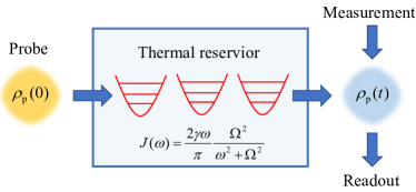
Figure 1: Schematic diagram of our quantum sensing scheme. A continuous-variable probe, which is initially prepared in a squeezed state, is employed to reveal the details of the spectral density $J(\omega)$ of a thermal reservoir, which consists of an infinite collection of noninteracting harmonic oscillators.

As displayed in Fig. 1, in our quantum sensing scheme, a harmonic oscillator is employed as the probe to detect the spectral density of a dissipative thermal reservoir. The whole Hamiltonian of the probe plus the reservoir can be described by $H=H_{\text{p}}+H_{\text{r}}+H_{\text{int}}+H_{\text{c}}$. Here

$$H_{\text{p}}=\frac{p^{2}}{2m}+\frac{1}{2}m\omega_{0}^{2}x^{2}$$ (3)

is the Hamiltonian of the probe,

$$H_{\text{r}}=\sum_{k}\bigg{(}\frac{p^{2}_{k}}{2m_{k}}+\frac{1}{2}m_{k}\omega_{k}^{2}x_{k}^{2}\bigg{)}$$ (4)

denotes the Hamiltonian of the thermal reservoir,

$$H_{\text{int}}=\sum_{k}c_{k}x_{k}\mathcal{S}$$ (5)

describes the probe-reservoir interaction, which is responsible for the encoding process in our sensing scheme, and

$$H_{\text{c}}=\sum_{k}\frac{c_{k}^{2}}{2m_{k}\omega_{k}^{2}}\mathcal{S}^{2}$$ (6)

is the so-called counter-term Breuer and Petruccione (Oxford University Press, Oxford, 2002), which compensates for the frequency shift induced by the interaction between the probe and the thermal reservoir Breuer and Petruccione (Oxford University Press, Oxford, 2002); Hu et al. (1992); Halliwell and Yu (1996); Ferialdi (2017). The quantities $\{x,p,m,\omega_{0}\}$ and $\{x_{k},p_{k},m_{k},\omega_{k}\}$ are the position, the momentum, the mass, and the frequency of the probe and the $k$th harmonic oscillator of the reservoir, respectively. Parameters $c_{k}$ quantify the probe-reservoir coupling strengths, and $\mathcal{S}$ denotes the coupling operator.

In this paper, we consider the following general coupling operator

$$\mathcal{S}=x\cos\theta+p\sin\theta.$$ (7)

By varying the coupling angle $\theta$, both position-position-type ($xx_{k}$-type) coupling and momentum-position-type ($px_{k}$-type) coupling can be taken into account. Notably, when $\theta=0$, the standard Caldeira-Leggett model Breuer and Petruccione (Oxford University Press, Oxford, 2002); Hu et al. (1992); Halliwell and Yu (1996); Ferialdi (2017) can be recovered. In Refs. Ferialdi and Smirne (2017); Ferialdi (2017), the authors reported that the momentum-position-type coupling can remarkably modify the dissipation experienced by the probe. Their results inspire us to explore the effect of the momentum-position-type coupling on the sensitivity of the quantum sensing.

The spectral density in our model, which is defined by

$$J(\omega)\equiv\sum_{k}\frac{c_{k}^{2}}{2m_{k}\omega_{k}}\delta(\omega-\omega_{k}),$$ (8)

fully determines the properties of the thermal reservoir. In the following, we assume $J(\omega)$ is an Ohmic spectral density with a Lorentz-Drude cutoff

$$J(\omega)=\frac{2\gamma\omega}{\pi}\frac{\Omega^{2}}{\omega^{2}+\Omega^{2}},$$ (9)

where $\gamma$ (the coupling strength) and $\Omega$ (the cutoff frequency) are the two parameters to be estimated in this paper, namely $\lambda=\gamma$ or $\Omega$ henceforth. The Ohmic-type spectral density constitutes a very general form to describe many different types of reservoirs. By varying the scopes of the coupling strength $\gamma$ and the cutoff frequency $\Omega$, the Ohmic-type spectral density can be employed to simulate the dynamics of charged interstitials in metals Leggett et al. (1987); de Vega and Alonso (2017). Moreover, an Ohmic model with a Lorenz-Drude regularization can be used to describe the electronic energy transfer dynamics in photosynthetic a pigment-protein complex and the Fenna-Matthews-Olson complex Ishizaki and Fleming (2009). On the other hand, the choice of the Lorentz-Drude-type Ohmic spectral density can greatly reduce the difficulties in deriving the expression of the output state. Thus, due to the above two reasons, we choose the Ohmic spectral density as the example to demonstrate the feasibility of our proposed sensing scheme.

The probe is initially prepared in a squeezed state

$$\rho_{\text{p}}(0)=S(r)D(\alpha)|0\rangle\langle 0|D^{\dagger}(\alpha)S^{\dagger}(r),$$ (10)

where $D(\alpha)\equiv\exp(\alpha a^{\dagger}-\alpha^{*}a)$ and $S(r)\equiv\exp[r(a^{2}-a^{{\dagger}2})/2]$ are the displacement and the squeeze operators, respectively. Here, $a|0\rangle=0$ denotes the Fock vacuum state and $a\equiv(x+ip)/\sqrt{2}$ is introduced as the annihilation operator of the probe. It is easy to prove that $\rho_{\text{p}}(0)$ is a Gaussian state. Assuming the whole initial state of the probe plus the reservoir is $\rho_{\text{p}}(0)\otimes\rho_{\text{r}}^{\text{G}}$ with $\rho_{\text{r}}^{\text{G}}=e^{-\beta H_{\text{r}}}/\text{Tr}(e^{-\beta H_{\text{r}}})$ being the canonical Gibbs state of the thermal reservoir, the dissipative dynamics generated by $H$ can be exactly derived by using the quantum master equation approach. As demonstrated in Refs. Breuer and Petruccione (Oxford University Press, Oxford, 2002); Ferialdi and Smirne (2017); Ferialdi (2017); Einsiedler et al. (2020), the Gaussianity of the probe can be fully preserved during the time evolution as a consequence of the bilinear structure of the global Hamiltonian $H$. On the other hand, using the Heisenberg equation of motion, the expressions of $\boldsymbol{d}$ and $\boldsymbol{\sigma}$ can be obtained (see Appendices A and B for details). As long as the first two momenta are obtained, the QFI can be accordingly computed by making use of Eq. (2).

When performing the numerical calculations to $\mathcal{F}_{\lambda}$ using Eq. (2), one needs to handle first-order derivatives, $\partial_{\lambda}\boldsymbol{d}$ and $\partial_{\lambda}\boldsymbol{\sigma}$ in Eq. (2). In this paper, the first-order derivative for an arbitrary $\lambda$-dependent function $f_{\lambda}$ is numerically done by adopting the following finite difference method (see Appendix C and Ref. Hofmann et al. (2014) for more details):

$$\partial_{\lambda}f_{\lambda}\simeq\frac{-f_{\lambda+2\delta}+8f_{\lambda+\delta}-8f_{\lambda-\delta}+f_{\lambda-2\delta}}{12\delta}.$$ (11)

We set $\delta/\lambda=10^{-6}$, which provides a very good accuracy.

III Results

III.1 Non-Markovian dynamics of the QFI

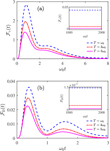
Figure 2: The non-Markovian dynamics of (a) $\mathcal{F}_{\gamma}(t)$ and (b) $\mathcal{F}_{\Omega}(t)$ with different temperatures: $T=\omega_{0}$ (blue dashed lines), $T=3\omega_{0}$ (red-dotdashed lines), and $T=5\omega_{0}$ (magenta solid lines). The insets depict the steady-state QFI $\mathcal{F}_{\lambda}(\infty)$ in the long-time regime. One can see that the value of $\mathcal{F}_{\lambda}(\infty)$ is small, but still positive. Other parameters are chosen as $\omega_{0}=0.5$ THz, $\Omega=10\omega_{0}$, $\gamma=3\omega_{0}$, $r=5\omega_{0}$, $\alpha=0$ and, $\theta=0$.

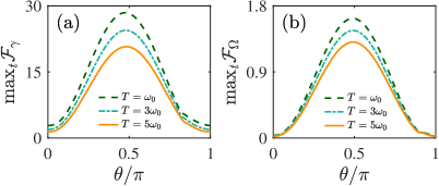
Figure 3: The maximal QFI of (a) $\max_{t}\mathcal{F}_{\gamma}$ and (b) $\max_{t}\mathcal{F}_{\Omega}$ are plotted as a function of the coupling angle $\theta$ with different temperatures: $T=\omega_{0}$ (green dashed lines), $T=3\omega_{0}$ (cyan-dotdashed lines), and $T=5\omega_{0}$ (orange solid lines). Due to the rotational symmetry of $\mathcal{S}$, we here restrict our study to $\theta\in[0,\pi]$. Other parameters are the same as those of Fig. 2.

The non-Markovian dynamical behavior of the QFI is displayed in Fig. 2. At the beginning, no message about the spectral density is included in the initial state $\rho_{\text{p}}(0)$, leading to $\mathcal{F}_{\lambda}(0)=0$. As the encoding time becomes longer, the probe-reservoir interaction generates the information of the spectral density, which results in the increase of the QFI. After arriving at a maximum value, $\mathcal{F}_{\lambda}(t)$ begins to decrease as a result of decoherence. Finally, as the probe evolves to its steady state $\rho_{\text{p}}(0)$ in the long-encoding-time limit, the value of $\mathcal{F}_{\lambda}(t)$ remains unchanged. In the inserts of Fig. 2, we plot the QFI in the long-encoding-time regime. One can clearly see $\mathcal{F}_{\lambda}(\infty)>0$, which is induced by the purely non-Markovian effect and is evidently different from that of the previous Markovian case Bina et al. (2018); Binder and Braun (2020); Monras and Paris (2007); Jarzyna and Zwierz (2017). More detailed discussions on the behavior of $\mathcal{F}_{\lambda}(\infty)$ are presented in the Sec. III.3.

The above result means there exists an optimal encoding time which can maximize the QFI. The occurrence of such a maximal QFI with respect to the optimal encoding time originates from the competition between the indispensable encoding and the unavoidable decoherence Wu et al. (2021); Zhang and Wu (2021), which are induced by the probe-reservoir interaction. In Fig. 3, we plot the maximal QFI, $\max_{t}\mathcal{F}_{\lambda}$, as a function of the coupling angle $\theta$. One can find that the maximal QFI can be further improved by adjusting the coupling angle. This result means the pure position-position-type coupling in the standard Caldeira-Leggett model is not the prime choice for obtaining the maximum sensing precision. Via adding the momentum-position-type coupling in $H_{\text{sb}}$, one can design the most efficient probe-reservoir interaction Hamiltonian for the encoding process.

Moreover, we observe that the dynamics of QFI can exhibit an oscillating behavior, e.g., the blue dashed line in Fig. 2 (b), which will result in multiple local maxima. This behavior is different from the previous result Bina et al. (2018) in which there exists one single peak. Such a result was also reported in Refs. Zhang and Wu (2021); Wu and Shi (2020) and may be linked to the exchange of information between the thermal reservoir and the probe. The reversed information flow from the reservoir back to the probe is commonly regarded as evidence of non-Markovianity.

III.2 The scaling relation

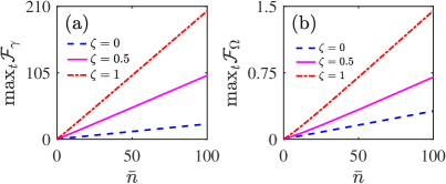
Figure 4: The maximum QFI of (a) $\max_{t}\mathcal{F}_{\gamma}$ and (b) $\max_{t}\mathcal{F}_{\Omega}$ vs the averaged number of photons, $\bar{n}$, with different squeezing ratios: $\zeta=0$ (blue dashed lines), $\zeta=0.5$ (magenta solid lines), and $\zeta=1$ (red dot-dashed lines). Other parameters are chosen as $\omega_{0}=1$ THz, $\Omega=10\omega_{0}$, $T=3\omega_{0}$, and $\gamma=\omega_{0}$.

For the initial state given by Eq. (10), the averaged photon number reads

$$\bar{n}\equiv\text{Tr}\big{[}\rho_{\text{p}}(0)a^{\dagger}a\big{]}=|\alpha|^{2}+\sinh^{2}r,$$ (12)

which can be regarded as the quantum resource employed in our sensing scheme. Furthermore, we introduce a squeezing ratio $\zeta\equiv\sinh^{2}r/\bar{n}$ to quantify the weight of quantum squeezing in the total quantum resource. The ratio of $\zeta$ varies from $\zeta=0$ for a purely coherent state to $\zeta=1$ for a purely squeezed vacuum state. Next, we shall explore the scaling relation versus $\bar{n}$ and $\zeta$.

The scaling relations between $\max_{t}\mathcal{F}_{\lambda}$ and $\bar{n}$ with different squeezing ratios are displayed in Fig. 4. One can find that $\max_{t}\mathcal{F}_{\lambda}$ is proportional to $\bar{n}$, which means the sensing precision scales as the SQL in our scheme. However, we find that the slope of the SQL can be enhanced by increasing the weight of quantum squeezing, which implies that quantum squeezing can be used as a resource to boost the sensing performance. These results are in agreement with many previous studies of noisy quantum metrology: in a noiseless ideal case, using quantum resource can indeed boost the metrological performance and result in a better scaling relation (such as the Zeno limit Caves (1981); Bai et al. (2019) or the Heisenberg limit Huelga et al. (1997)), but these quantum superiorities generally degrade back to the SQL under the influence of decoherence Wu et al. (2021); Wang et al. (2017); Matsuzaki et al. (2018); Chin et al. (2012). Such a result is called the no-go theorem of noisy quantum metrology.

III.3 Breakdown of the Markovian approximation in the long-encoding-time regime

Figure 5: The steady-state second moments of (a) $\sigma_{xx}(\infty)$ and (b) $\sigma_{pp}(\infty)$ are plotted as a function of temperature. The steady-state QFIs of (c) $\mathcal{F}_{\gamma}(\infty)$ and (d) $\mathcal{F}_{\Omega}(\infty)$ are displayed with the increase of temperature. The red five-pointed stars are Markovian results, while the blue crosses represent the results predicted by our non-Markovian method. Other parameters are chosen as $\omega_{0}=0.5~{}\text{THz}$, $\Omega=10\omega_{0}$, $\gamma=3\omega_{0}$, $r=\omega_{0}$, $\alpha=0$, and $\theta=0$.

In this subsection, we shall discuss the steady-state QFI in the long-encoding-time regime. As demonstrated in many previous works Breuer and Petruccione (Oxford University Press, Oxford, 2002); Yang et al. (2014); Cai et al. (2014); Iles-Smith et al. (2014); Lee et al. (2012); Xiong et al. (2015), within the Markovian treatment, the long-time steady state of the probe can be described by a canonical Gibbs state at the same temperature as the quantum reservoir. On the other hand, the contribution from the counter term $H_{\text{c}}$ is completely washed out by the probe-reservoir interaction under the Markovian approximation Breuer and Petruccione (Oxford University Press, Oxford, 2002). The above two points mean the steady state of the probe will be

$$\rho_{\text{p}}(\infty)=\rho_{\text{p}}^{\text{G}}=\frac{e^{-\beta H_{\text{p}}}}{\text{Tr}(e^{-\beta H_{\text{p}}})},$$ (13)

instead of $\rho_{\text{p}}(\infty)\propto e^{-\beta(H_{\text{p}}+H_{\text{c}})}$. This result is quite different from that of the qubit-based temperature sensing case Zhang and Wu (2021), in which the effect of frequency renormalization is fully included in the steady state of the probe. From the above Eq. (13), one can easily find $\boldsymbol{d}_{\text{M}}(\infty)=(0,0)^{\text{T}}$ and

$$\boldsymbol{\sigma}_{\text{M}}(\infty)=\coth\Big{(}\frac{\omega_{0}}{2T}\Big{)}\left(\begin{array}[]{cc}\omega_{0}^{-1}&0\\ 0&\omega_{0}\\ \end{array}\right)$$ (14)

are independent of the details of the spectral density, which leads to $\mathcal{F}_{\lambda}^{\text{M}}(\infty)=0$. It is necessary to point out that $\boldsymbol{d}_{\text{M}}(\infty)=(0,0)^{\text{T}}$ and Eq. (14) can be reproduced by directly calculating the equilibration dynamics of the probe under the Markovian approximation (see Appendix B for details).

However, such a canonical thermalization totally breaks down, namely, $\rho_{\text{p}}(\infty)\neq\rho_{\text{p}}^{\text{G}}$, in the strongly non-Markovian regime where the noncanonical equilibrium state appears. As demonstrated in Refs. Iles-Smith et al. (2014); Lee et al. (2012), the emergence of a noncanonical distribution is commonly linked to the existence of probe-reservoir correlations, which implies there exists information exchange between the probe and the thermal reservoir. This result suggests, in the non-Markovian case, the long-time steady state of the probe will rely on not only the reservoir’s temperature, but also the details of the spectral density, resulting in $\mathcal{F}_{\lambda}(\infty)>0$.

To check the above analysis, in Figs. 5(a) and  5(b), we display $\sigma_{xx}(\infty)$ and $\sigma_{pp}(\infty)$ versus the temperature of the quantum reservoir from using the non-Markovian and the Markovian methods. One can find that the non-Markovian results depart from the results predicted by the canonical Gibbs state when temperature is very low, for example, $T/\omega_{0}\in(0,2]$ in Fig. 5(b). This result means the breakdown of the Markovian approximation and the appearance of the noncanonical equilibration in the low-temperature regime. In Figs. 5(c) and  5(d), $\mathcal{F}_{\lambda}(\infty)$ is plotted as a function of the temperature. One can see $\mathcal{F}_{\lambda}(\infty)>0$ if the temperature is very low. However, with increasing temperature, the non-Markovianity becomes ignorable and $\mathcal{F}_{\lambda}(\infty)$ gradually vanishes. In this sense, the non-zero residual QFI at low temperature stems from non-Markovian effects which cannot be predicted by the previous Markovian approaches Bina et al. (2018); Binder and Braun (2020); Monras and Paris (2007); Jarzyna and Zwierz (2017). This result means the non-Markovianity is not only a mathematical concept, but also a valuable resource to improve the sensing precision.

III.4 Enhanced sensing performance by adding an external driving field

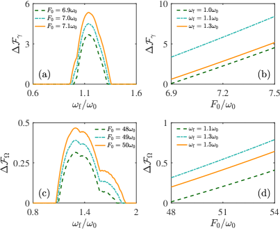
Figure 6: $\Delta\mathcal{F}_{\gamma}$ is plotted as a function of (a) the driving frequency $\omega_{\rm f}$ and (b) the driving amplitude $F_{0}$. $\Delta\mathcal{F}_{\Omega}$ vs (c) the driving frequency $\omega_{\rm f}$ and (d) the driving amplitude $F_{0}$. Parameters are chosen as $\omega_{0}=0.5~{}\text{THz}$, $\Omega=10\omega_{0}$, $\gamma=3\omega_{0}$, $r=5\omega_{0}$, $\alpha=0$, and $\theta=\theta_{\text{opt}}$.

In this subsection, we present a dynamical steer protocol to improve the sensing performance by using an external driving field, which is solely applied to the probe. To this aim, in the original Hamiltonian of the probe, we add the following time-dependent term Golovinski (2020); Xu et al. (2009)

$$H_{\text{f}}(t)=-F_{0}\sin(\omega_{\text{f}}t)x,$$ (15)

where $F_{0}$ and $\omega_{\text{f}}$ are the driving amplitude and frequency, respectively. Using the method of deriving the first two moments given in Appendix A, the QFI under driving can be obtained without difficulties. To quantify the influences of the continuous-wave driving field on the sensing precision, we define the following quantity:

$$\Delta\mathcal{F}_{\lambda}\equiv\max_{t}\mathcal{F}_{\lambda}(F_{0},\omega_{\text{f}})-\max_{t}\mathcal{F}_{\lambda}(F_{0}=0,\omega_{\text{f}}=0).$$ (16)

As long as $\Delta\mathcal{F}_{\lambda}>0$, one can conclude that the external driving field plays a positive role in our sensing performance. As shown in Fig. 6, via applying an external driving field, the sensing precision can be effectively improved. Moreover, by adjusting either the driving amplitude $F_{0}$ or the frequency $\omega_{\text{f}}$, the effect of the external driving field can be further optimized. From Fig. 6, one can see that the constructive effect generated by optimizing the driving amplitude is rather robust: $\Delta\mathcal{F}_{\lambda}$ scales linearly with the increase of the value of $F_{0}$. However, when the driving frequency $\omega_{\text{f}}$ is neither too high nor too low, the dynamical steer effect induced by varying the driving frequency $\omega_{\text{f}}$ becomes negligible.

IV Conclusion

In summary, we employ a harmonic oscillator, which is initially prepared in a squeezed state, acted as a probe to estimate the parameters of the spectral density of a bosonic reservoir. Going beyond the usual Markovian treatment, a SQL-type scaling relation, which can be further optimized by increasing the proportion of squeezing in the initial quantum resource, is revealed. To maximize the sensing precision, we analyze the influences of the form of probe-reservoir interaction, the non-Markovianity as well as an external driving field on the sensing performance. It is found that the sensing sensitivity the can be significantly improved by including $px_{k}$-type coupling, which is commonly neglected in the standard Caldeira-Leggett model. At low temperature, we find that the non-Markovianity can lead to a noncanonical equilibrium state, which contains information of the spectral density under the influence of decoherence. Using such a non-Markovian effect, our sensing scheme still works in the long-encoding-time regime where the Markovian one completely breaks down. Moreover, we propose a dynamical steer protocol, in which an external driving field is applied to the probe, to boost the sensing outcome. Our results presented in this paper may provide some theory supports for designing a high-precision quantum sensor. Furthermore, due to the importance of the spectral density in the theory of open quantum systems, we expect our results to be of interest for understanding and controlling the decoherence.

V Acknowledgments

The authors thank Dr. Si-Yuan Bai, Dr. Chong Chen, Professor Jun-Hong An and Professor Hong-Gang Luo for many fruitful discussions. The work was supported by the National Natural Science Foundation (Grants No. 11704025 and No. 12047501).

VI Appendix A: The exact expressions of $\boldsymbol{d}$ and $\boldsymbol{\sigma}$

In this appendix, we would like to show how to derive exact expressions of $\boldsymbol{d}$ and $\boldsymbol{\sigma}$. Using the Heisenberg equation of motion of $\mathcal{\dot{O}}=-i[\mathcal{O},H]$, one can find that the equations of motion of $x$, $x_{k}$, $p$, and $p_{k}$ are given by ($m=1$)

$$\dot{x}=p+\sin\theta\bigg{(}\sum_{k}c_{k}x_{k}+\sum_{k}\frac{c_{k}^{2}}{m_{k}\omega_{k}^{2}}\mathcal{S}\bigg{)},$$ (17)

$$\dot{p}=-\omega_{0}^{2}x-\cos\theta\bigg{(}\sum_{k}c_{k}x_{k}+\sum_{k}\frac{c_{k}^{2}}{m_{k}\omega_{k}^{2}}\mathcal{S}\bigg{)},$$ (18)

$$\dot{x}_{k}=\frac{p_{k}}{m_{k}},~{}~{}~{}\dot{p}_{k}=-m_{k}\omega_{k}^{2}x_{k}-c_{k}\mathcal{S}.$$ (19)

From Eq. (19), one can find that the formal solution of $x_{k}$ is

$$x_{k}(t)=x_{k}(0)\cos(\omega_{k}t)+\frac{p_{k}(0)}{m_{k}\omega_{k}}\sin(\omega_{k}t)-\sum_{k}\frac{c_{k}}{m_{k}\omega_{k}}\int_{0}^{t}d\tau\sin[\omega_{k}(t-\tau)]\mathcal{S}(\tau),$$ (20)

where $\mathcal{S}(t)=x(t)\cos\theta+p(t)\sin\theta$. Substituting the above formal solution of $x_{k}$ into Eqs. (17) and  (18), one can find the following integro-differential equation for the position operator :

$$\ddot{x}(t)+\omega_{0}^{2}x(t)+\bigg{(}\cos\theta\frac{d}{dt}-\sin\theta\frac{d^{2}}{dt^{2}}\bigg{)}\int_{0}^{t}d\tau\mathcal{Z}(t-\tau)\mathcal{S}(\tau)=\sin\theta\mathcal{\dot{R}}(t)-\cos\theta\mathcal{R}(t),$$ (21)

where

$$\mathcal{Z}(t)\equiv\sum_{k}\frac{c_{k}^{2}}{m_{k}\omega_{k}^{2}}\cos(\omega_{k}t),~{}~{}~{}\mathcal{R}(t)\equiv\sum_{k}c_{k}\bigg{[}x_{k}(0)\cos(\omega_{k}t)+\frac{p_{k}(0)}{m_{k}\omega_{k}}\sin(\omega_{k}t)\bigg{]},$$ (22)

are, respectively, the so-called damping kernel and environment-induced stochastic force. In this paper, we consider the reservoir to be initially prepared as $\rho_{\text{r}}^{\text{G}}=e^{-\beta H_{\text{r}}}/\text{Tr}(e^{-\beta H_{\text{r}}})$. This assumption leads to $\langle\mathcal{R}(t)\rangle_{\text{r}}=0$ and the symmetrized environmental correlation function is given by

$$\mathcal{C}(t)\equiv\frac{1}{2}\Big{[}\langle\mathcal{R}(t)\mathcal{R}(0)\rangle_{\text{r}}+\langle\mathcal{R}(0)\mathcal{R}(t)\rangle_{\text{r}}\Big{]}=\sum_{k}\frac{c_{k}^{2}}{2m_{k}\omega_{k}^{2}}\coth\Big{(}\frac{\beta\omega_{k}}{2}\Big{)}\cos(\omega_{k}t),$$ (23)

where $\langle\mathcal{O}\rangle_{\text{r}}\equiv\text{Tr}_{\text{b}}(\rho_{\text{r}}^{\text{G}}\mathcal{O})$. For the Ohmic spectral density considered in this paper, one can find $\mathcal{Z}(t)=\gamma\Omega e^{-\Omega t}$ and

$$\begin{split}\mathcal{C}(t)=&\frac{2\gamma}{\beta}e^{-\Omega t}+\frac{4\gamma\Omega^{2}}{\beta}\sum_{n=1}^{\infty}\frac{\nu_{n}e^{-\nu_{n}t}-\Omega e^{-\Omega t}}{\nu_{n}^{2}-\Omega^{2}}=\frac{2\gamma}{\beta}e^{-\Omega t}-\frac{4\gamma\Omega^{2}}{\beta}\sum_{n=1}^{\infty}\frac{\Omega e^{-\Omega t}}{\nu_{n}^{2}-\Omega^{2}}+\frac{4\gamma\Omega^{2}}{\beta}\sum_{n=1}^{\infty}\frac{\nu_{n}e^{-\nu_{n}t}}{\nu_{n}^{2}-\Omega^{2}}\\ =&\frac{\gamma}{\beta}\bigg{[}2(1-\Omega)+\beta\Omega^{2}\cot\Big{(}\frac{\beta\Omega}{2}\Big{)}\bigg{]}e^{-\Omega t}+\frac{\gamma\Omega^{2}}{\pi}\bigg{[}\mathbb{H}\Big{(}e^{-\frac{2\pi t}{\beta}},1,1-\frac{\beta\Omega}{2\pi}\Big{)}+\mathbb{H}\Big{(}e^{-\frac{2\pi t}{\beta}},1,1+\frac{\beta\Omega}{2\pi}\Big{)}\bigg{]}e^{-\frac{2\pi t}{\beta}},\end{split}$$ (24)

where $\nu_{n}\equiv 2n\pi/\beta$ are the Matsubara frequencies, and $\mathbb{H}(a,b,c)$ denotes the Lerch transcendent function.

Solving the Eq. (21) by using Laplace transformation, one can find

$$x(t)=\mathcal{G}_{1}(t)x(0)+\mathcal{G}_{2}(t)p(0)+\int_{0}^{t}d\tau\mathcal{G}_{3}(t-\tau)\mathcal{R}(\tau),$$ (25)

$$p(t)=\mathcal{G}_{4}(t)x(0)+\mathcal{G}_{5}(t)p(0)+\int_{0}^{t}d\tau\mathcal{G}_{6}(t-\tau)\mathcal{R}(\tau).$$ (26)

Here, $\mathcal{G}_{\alpha}(t)$ with $\alpha=1,2,3,4,5,6$ are determined by the following inverse Laplace transformation

$$\mathcal{G}_{1}(t)=\mathcal{L}^{-1}\Bigg{[}\frac{z+z\cos\theta\sin\theta\tilde{\mathcal{Z}}(z)}{\zeta(z)}\Bigg{]},~{}~{}\mathcal{G}_{2}(t)=\mathcal{L}^{-1}\Bigg{[}\frac{1+z\sin^{2}\theta\tilde{\mathcal{Z}}(z)}{\zeta(z)}\Bigg{]},~{}~{}\mathcal{G}_{3}(t)=\mathcal{L}^{-1}\Bigg{[}\frac{z\sin\theta-\cos\theta}{\zeta(z)}\Bigg{]},$$ (27)

$$\mathcal{G}_{4}(t)=\mathcal{L}^{-1}\Bigg{[}\frac{-\omega_{0}^{2}-z\cos^{2}\theta\tilde{\mathcal{Z}}(z)}{\zeta(z)}\Bigg{]},~{}~{}\mathcal{G}_{5}(t)=\mathcal{L}^{-1}\Bigg{[}\frac{z-z\sin\theta\cos\theta\tilde{\mathcal{Z}}(z)}{\zeta(z)}\Bigg{]},~{}~{}\mathcal{G}_{6}(t)=\mathcal{L}^{-1}\Bigg{[}\frac{-\omega_{0}^{2}\sin\theta-z\cos\theta}{\zeta(z)}\Bigg{]},$$ (28)

where $\zeta(z)\equiv\omega_{0}^{2}+z^{2}+z\tilde{\mathcal{Z}}(z)(\cos^{2}\theta+\omega_{0}^{2}\sin^{2}\theta)$ and $\mathcal{Z}(z)=\mathcal{L}[\mathcal{Z}(t)]=\gamma\Omega/(z+\Omega)$. By making use of residue theorem, the inverse Laplace transformation can be exactly worked out:

$$\mathcal{G}_{\alpha}(t)=\sum_{\text{i}\neq\text{j}\neq\text{k}=1}^{3}\frac{G_{\alpha}(z_{\text{i}})e^{z_{\text{i}}t}}{(z_{\text{i}}-z_{\text{j}})(z_{\text{i}}-z_{\text{k}})},$$ (29)

where $z_{\text{i}}$ are the roots of the cubic polynomial $z^{3}+\Omega z^{2}+[\omega_{0}^{2}+\gamma\Omega(\cos^{2}\theta+\omega_{0}^{2}\sin^{2}\theta)]z+\omega_{0}^{2}\Omega=0$, and $G_{\alpha}(z)$ are given by

$$G_{1}(z)=z(z+\Omega)+z\gamma\Omega\cos\theta\sin\theta,~{}~{}G_{2}(z)=z+\Omega+z\gamma\Omega\sin^{2}\theta,~{}~{}G_{3}(z)=(z+\Omega)(z\sin\theta-\cos\theta),$$ (30)

$$G_{4}(z)=-\omega_{0}^{2}(z+\Omega)-z\gamma\Omega\cos^{2}\theta,~{}~{}G_{5}(z)=z(z+\Omega)-z\gamma\Omega\cos\theta\sin\theta,~{}~{}G_{6}(z)=-(z+\Omega)(\omega_{0}\sin\theta+z\cos\theta).$$ (31)

Using Eqs. (25),  (26), and some straightforward calculations, we can finally obtain the exact expressions of the first two momentums as $d_{x,p}=\mathcal{G}_{1,4}(t)\langle x(0)\rangle_{\text{p}}+\mathcal{G}_{2,5}(t)\langle p(0)\rangle_{\text{p}}$ and

$$\sigma_{xx}(t)=\mathcal{G}_{1}^{2}(t)\sigma_{xx}(0)+\mathcal{G}_{2}^{2}(t)\sigma_{pp}(0)+2\mathcal{G}_{1}(t)\mathcal{G}_{2}(t)\sigma_{xp}(0)+2\int_{0}^{t}d\tau\int_{0}^{t}d\tau^{\prime}\mathcal{G}_{3}(t-\tau)\mathcal{G}_{3}(t-\tau^{\prime})\mathcal{C}(\tau-\tau^{\prime}),$$ (32)

$$\sigma_{pp}(t)=\mathcal{G}_{4}^{2}(t)\sigma_{xx}(0)+\mathcal{G}_{5}^{2}(t)\sigma_{pp}(0)+2\mathcal{G}_{4}(t)\mathcal{G}_{5}(t)\sigma_{xp}(0)+2\int_{0}^{t}d\tau\int_{0}^{t}d\tau^{\prime}\mathcal{G}_{6}(t-\tau)\mathcal{G}_{6}(t-\tau^{\prime})\mathcal{C}(\tau-\tau^{\prime}),$$ (33)

$$\begin{split}\sigma_{xp}(t)=&\mathcal{G}_{1}(t)\mathcal{G}_{4}(t)\sigma_{xx}(0)+\mathcal{G}_{2}(t)\mathcal{G}_{5}(t)\sigma_{pp}(0)+2[\mathcal{G}_{2}(t)\mathcal{G}_{4}(t)+\mathcal{G}_{1}(t)\mathcal{G}_{5}(t)]\sigma_{xp}(0)\\ &+2\int_{0}^{t}d\tau\int_{0}^{t}d\tau^{\prime}\mathcal{G}_{3}(t-\tau)\mathcal{G}_{6}(t-\tau^{\prime})\mathcal{C}(\tau-\tau^{\prime}),\end{split}$$ (34)

where $\langle\mathcal{O}\rangle_{\text{p}}\equiv\text{Tr}_{\text{p}}[\rho_{\text{p}}(0)\mathcal{O}]$ and $\sigma_{ij}(0)$ denotes the initial covariant matrix with respect to $\rho_{\text{p}}(0)$.

VII Appendix B: Markovian results

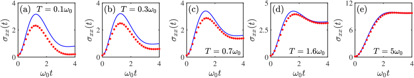
Figure 7: The dynamics of the second moment $\sigma_{xx}(t)$ with different temperatures: (a) $T=0.1\omega_{0}$, (b) $T=0.3\omega_{0}$, (c) $T=0.7\omega_{0}$, (d) $T=1.6\omega_{0}$, (e) $T=5\omega_{0}$. The red hexagons are the Markovian results, while the blue solid lines are obtained by the non-Markovian method. Other parameters are chosen as $\omega_{0}=1~{}\text{THz}$, $\Omega=10\omega_{0}$, $\gamma=\omega_{0}$, $r=\omega_{0}$, $\alpha=0$, and $\theta=0$.

In the case of $\gamma,\omega_{0}\ll\text{min}\{\Omega,2\pi T\}$, Refs. Breuer and Petruccione (Oxford University Press, Oxford, 2002); Einsiedler et al. (2020) provided a Markovian approximate expressions of $\mathcal{G}_{\alpha}(t)$ in the case of $\theta=0$ as follows:

$$\mathcal{G}_{1}^{\text{M}}(t)\simeq\bigg{[}\frac{\kappa}{\Lambda}\sin(\Lambda t)+\cos(\Lambda t)\bigg{]}e^{-\kappa t},~{}~{}\mathcal{G}_{2}^{\text{M}}(t)\simeq\frac{1}{\Lambda}\sin(\Lambda t)e^{-\kappa t},~{}~{}\mathcal{G}_{3}^{\text{M}}(t)\simeq-\frac{1}{\Lambda}\sin(\Lambda t)e^{-\kappa t},$$ (35)

$$\mathcal{G}_{4}^{\text{M}}(t)\simeq-\frac{\omega_{0}^{2}}{\Lambda}\sin(\Lambda t)e^{-\kappa t},~{}~{}\mathcal{G}_{5}^{\text{M}}(t)\simeq\cos(\Lambda t)e^{-\kappa t}-\frac{\kappa}{\Lambda}\sin(\Lambda t)e^{-\kappa t},~{}~{}\mathcal{G}_{6}^{\text{M}}(t)\simeq-\cos(\Lambda t)e^{-\kappa t}+\frac{\kappa}{\Lambda}\sin(\Lambda t)e^{-\kappa t},$$ (36)

where $\kappa\equiv\gamma/2$ and $\Lambda^{2}\equiv\omega_{0}^{2}-\kappa^{2}$. On the other hand, in the Markovian treatment, the environmental correlation function $\mathcal{C}(\tau-\tau^{\prime})$ reduces to a Dirac-$\delta$ function, i.e., $\mathcal{C}_{\text{M}}(\tau-\tau^{\prime})\simeq 4\gamma T\delta(\tau-\tau^{\prime})$. With these above approximate expressions of $\mathcal{G}_{\alpha}^{\text{M}}(t)$ and $\mathcal{C}_{\text{M}}(\tau-\tau^{\prime})$ at hand, the first two momentums under the Markovian approximation can easily be obtained. In Fig. 7, we display $\sigma_{xx}(t)$ from both the Markovian and non-Markovian methods. Good agreement is found between results from the above two different approaches at high temperature, say $T=5\omega_{0}$ in Fig. 7(e). However, as the environmental temperature decreases, the non-Markovian effect becomes strong. At low temperature, e.g., $T=0.1\omega_{0}$ in Fig. 7(a), a relatively large deviation is found, which means the breakdown of the Markovian approximation. Moreover, using Eqs. (35),  (36), and the Dirac-$\delta$-type environmental correlation function, one can easily derive the expressions of the first two momentums in the long-encoding-limit, which recovers $\boldsymbol{d}_{\text{M}}(\infty)=(0,0)^{\text{T}}$ and Eq. (14) in the main text. This result demonstrate that the probe experiences a canonical thermalization under the Markovian approximation, which is consistent with Refs. Yang et al. (2014); Cai et al. (2014); Iles-Smith et al. (2014); Lee et al. (2012).

VIII Appendix C: The derivation of Eq. (11)

In this appendix, we show the details of deriving the Eq. (11). By making the Lagrange interpolation method, a smooth function $f_{\lambda}=f(\lambda)$, which is defined in a tiny interval $\lambda\in[\lambda_{\text{min}},\lambda_{\text{max}}]$, can be approximately expressed as a sum of polynomials,

$$f(\lambda)\simeq\sum_{\text{n}=0}^{N}f(\lambda_{\text{n}})\mathbb{L}_{\text{n}}(x),$$ (37)

where $\lambda_{\text{min}}=\lambda_{0}<\lambda_{1}<...<\lambda_{N}=\lambda_{\text{max}}$ with $\lambda_{\text{n}+1}=\lambda_{\text{n}}+\delta$; $\delta=(\lambda_{\text{max}}-\lambda_{\text{min}})/N$ are $(N+1)$ uniformly spaced nodes; and

$$\mathbb{L}_{\text{n}}(x)\equiv\prod_{\text{m}\neq\text{n}}\frac{x-x_{\text{m}}}{x_{\text{n}}-x_{\text{m}}}$$ (38)

is the so-called Lagrange multiplier function. Taking $N=4$ as an example, we have

$$\begin{split}f(\lambda)\simeq&\frac{(\lambda-\lambda_{1})(\lambda-\lambda_{2})(\lambda-\lambda_{3})(\lambda-\lambda_{4})}{(\lambda_{0}-\lambda_{1})(\lambda_{0}-\lambda_{2})(\lambda_{0}-\lambda_{3})(\lambda_{0}-\lambda_{4})}f(\lambda_{0})+\frac{(\lambda-\lambda_{0})(\lambda-\lambda_{2})(\lambda-\lambda_{3})(\lambda-\lambda_{4})}{(\lambda_{1}-\lambda_{0})(\lambda_{1}-\lambda_{2})(\lambda_{1}-\lambda_{3})(\lambda_{1}-\lambda_{4})}f(\lambda_{1})\\ &+\frac{(\lambda-\lambda_{0})(\lambda-\lambda_{1})(\lambda-\lambda_{3})(\lambda-\lambda_{4})}{(\lambda_{2}-\lambda_{0})(\lambda_{2}-\lambda_{1})(\lambda_{2}-\lambda_{3})(\lambda_{2}-\lambda_{4})}f(\lambda_{2})+\frac{(\lambda-\lambda_{0})(\lambda-\lambda_{1})(\lambda-\lambda_{2})(\lambda-\lambda_{4})}{(\lambda_{3}-\lambda_{0})(\lambda_{3}-\lambda_{1})(\lambda_{3}-\lambda_{2})(\lambda_{3}-\lambda_{4})}f(\lambda_{3})\\ &+\frac{(\lambda-\lambda_{0})(\lambda-\lambda_{1})(\lambda-\lambda_{2})(\lambda-\lambda_{3})}{(\lambda_{4}-\lambda_{0})(\lambda_{4}-\lambda_{1})(\lambda_{4}-\lambda_{2})(\lambda_{4}-\lambda_{3})}f(\lambda_{4}).\end{split}$$ (39)

Assuming $f(\lambda)$ is differentiable in the interval of $[\lambda_{2}-2\delta,\lambda_{2}+2\delta]$, then the first-order derivative evaluated at $\lambda=\lambda_{2}$ can be approximately written as

$$\begin{split}f^{\prime}(\lambda_{2})\simeq\frac{d}{d\lambda}f(\lambda)\bigg{|}_{\lambda=\lambda_{2}}=\frac{1}{12\delta}[f(\lambda_{0})-8f(\lambda_{1})+8f(\lambda_{3})-f(\lambda_{4})],\end{split}$$ (40)

which recovers Eq. (11) in the main text.

References

- Degen et al. (2017) C. L. Degen, F. Reinhard, and P. Cappellaro, “Quantum sensing,” Rev. Mod. Phys. 89, 035002 (2017).
- Pezzè et al. (2018) Luca Pezzè, Augusto Smerzi, Markus K. Oberthaler, Roman Schmied, and Philipp Treutlein, “Quantum metrology with nonclassical states of atomic ensembles,” Rev. Mod. Phys. 90, 035005 (2018).
- Sidhu and Kok (2020) Jasminder S. Sidhu and Pieter Kok, “Geometric perspective on quantum parameter estimation,” AVS Quantum Science 2, 014701 (2020).
- Lachance-Quirion et al. (2020) Dany Lachance-Quirion, Samuel Piotr Wolski, Yutaka Tabuchi, Shingo Kono, Koji Usami, and Yasunobu Nakamura, “Entanglement-based single-shot detection of a single magnon with a superconducting qubit,” Science 367, 425–428 (2020).
- Megidish et al. (2019) Eli Megidish, Joseph Broz, Nicole Greene, and Hartmut Häffner, “Improved test of local lorentz invariance from a deterministic preparation of entangled states,” Phys. Rev. Lett. 122, 123605 (2019).
- Unternährer et al. (2018) Manuel Unternährer, Bänz Bessire, Leonardo Gasparini, Matteo Perenzoni, and André Stefanov, “Super-resolution quantum imaging at the heisenberg limit,” Optica 5, 1150–1154 (2018).
- Zou et al. (2018) Yi-Quan Zou, Ling-Na Wu, Qi Liu, Xin-Yu Luo, Shuai-Feng Guo, Jia-Hao Cao, Meng Khoon Tey, and Li You, “Beating the classical precision limit with spin-1 dicke states of more than 10,000 atoms,” Proceedings of the National Academy of Sciences 115, 6381–6385 (2018).
- Nagata et al. (2007) Tomohisa Nagata, Ryo Okamoto, Jeremy L. O’Brien, Keiji Sasaki, and Shigeki Takeuchi, “Beating the standard quantum limit with four-entangled photons,” Science 316, 726–729 (2007).
- Haine and Hope (2020) Simon A. Haine and Joseph J. Hope, “Machine-designed sensor to make optimal use of entanglement-generating dynamics for quantum sensing,” Phys. Rev. Lett. 124, 060402 (2020).
- Yamamoto et al. (2022) Kaoru Yamamoto, Suguru Endo, Hideaki Hakoshima, Yuichiro Matsuzaki, and Yuuki Tokunaga, “Error-mitigated quantum metrology,” (2022), arXiv:2112.01850 [quant-ph] .
- Caves (1981) Carlton M. Caves, “Quantum-mechanical noise in an interferometer,” Phys. Rev. D 23, 1693–1708 (1981).
- Baamara et al. (2021) Youcef Baamara, Alice Sinatra, and Manuel Gessner, “Scaling laws for the sensitivity enhancement of non-gaussian spin states,” Phys. Rev. Lett. 127, 160501 (2021).
- Nolan et al. (2017) Samuel P. Nolan, Stuart S. Szigeti, and Simon A. Haine, “Optimal and robust quantum metrology using interaction-based readouts,” Phys. Rev. Lett. 119, 193601 (2017).
- Liu et al. (2019a) Shengshuai Liu, Yanbo Lou, and Jietai Jing, “Interference-induced quantum squeezing enhancement in a two-beam phase-sensitive amplifier,” Phys. Rev. Lett. 123, 113602 (2019a).
- Tse and et al (2019) M. Tse and et al, “Quantum-enhanced advanced ligo detectors in the era of gravitational-wave astronomy,” Phys. Rev. Lett. 123, 231107 (2019).
- Branford et al. (2018) Dominic Branford, Haixing Miao, and Animesh Datta, “Fundamental quantum limits of multicarrier optomechanical sensors,” Phys. Rev. Lett. 121, 110505 (2018).
- Ma and Wang (2009) Jian Ma and Xiaoguang Wang, “Fisher information and spin squeezing in the lipkin-meshkov-glick model,” Phys. Rev. A 80, 012318 (2009).
- Invernizzi et al. (2008) Carmen Invernizzi, Michael Korbman, Lorenzo Campos Venuti, and Matteo G. A. Paris, “Optimal quantum estimation in spin systems at criticality,” Phys. Rev. A 78, 042106 (2008).
- Zanardi et al. (2008) Paolo Zanardi, Matteo G. A. Paris, and Lorenzo Campos Venuti, “Quantum criticality as a resource for quantum estimation,” Phys. Rev. A 78, 042105 (2008).
- Garbe et al. (2020) Louis Garbe, Matteo Bina, Arne Keller, Matteo G. A. Paris, and Simone Felicetti, “Critical quantum metrology with a finite-component quantum phase transition,” Phys. Rev. Lett. 124, 120504 (2020).
- Chu et al. (2021) Yaoming Chu, Shaoliang Zhang, Baiyi Yu, and Jianming Cai, “Dynamic framework for criticality-enhanced quantum sensing,” Phys. Rev. Lett. 126, 010502 (2021).
- Frérot and Roscilde (2018) Irénée Frérot and Tommaso Roscilde, “Quantum critical metrology,” Phys. Rev. Lett. 121, 020402 (2018).
- Bouton et al. (2020) Quentin Bouton, Jens Nettersheim, Daniel Adam, Felix Schmidt, Daniel Mayer, Tobias Lausch, Eberhard Tiemann, and Artur Widera, “Single-atom quantum probes for ultracold gases boosted by nonequilibrium spin dynamics,” Phys. Rev. X 10, 011018 (2020).
- Zhang and Wu (2021) Ze-Zhou Zhang and Wei Wu, “Non-markovian temperature sensing,” Phys. Rev. Research 3, 043039 (2021).
- Jørgensen et al. (2020) Mathias R. Jørgensen, Patrick P. Potts, Matteo G. A. Paris, and Jonatan B. Brask, “Tight bound on finite-resolution quantum thermometry at low temperatures,” Phys. Rev. Research 2, 033394 (2020).
- Correa et al. (2017) Luis A. Correa, Martí Perarnau-Llobet, Karen V. Hovhannisyan, Senaida Hernández-Santana, Mohammad Mehboudi, and Anna Sanpera, “Enhancement of low-temperature thermometry by strong coupling,” Phys. Rev. A 96, 062103 (2017).
- Płodzień et al. (2018) Marcin Płodzień, Rafał Demkowicz-Dobrzański, and Tomasz Sowiński, “Few-fermion thermometry,” Phys. Rev. A 97, 063619 (2018).
- Correa et al. (2015) Luis A. Correa, Mohammad Mehboudi, Gerardo Adesso, and Anna Sanpera, “Individual quantum probes for optimal thermometry,” Phys. Rev. Lett. 114, 220405 (2015).
- Hou et al. (2021) Zhibo Hou, Yan Jin, Hongzhen Chen, Jun-Feng Tang, Chang-Jiang Huang, Haidong Yuan, Guo-Yong Xiang, Chuan-Feng Li, and Guang-Can Guo, ““super-heisenberg” and heisenberg scalings achieved simultaneously in the estimation of a rotating field,” Phys. Rev. Lett. 126, 070503 (2021).
- Troullinou et al. (2021) C. Troullinou, R. Jiménez-Martínez, J. Kong, V. G. Lucivero, and M. W. Mitchell, “Squeezed-light enhancement and backaction evasion in a high sensitivity optically pumped magnetometer,” Phys. Rev. Lett. 127, 193601 (2021).
- Evrard et al. (2019) Alexandre Evrard, Vasiliy Makhalov, Thomas Chalopin, Leonid A. Sidorenkov, Jean Dalibard, Raphael Lopes, and Sylvain Nascimbene, “Enhanced magnetic sensitivity with non-gaussian quantum fluctuations,” Phys. Rev. Lett. 122, 173601 (2019).
- Razzoli et al. (2019) Luca Razzoli, Luca Ghirardi, Ilaria Siloi, Paolo Bordone, and Matteo G. A. Paris, “Lattice quantum magnetometry,” Phys. Rev. A 99, 062330 (2019).
- Wu et al. (2021) Wei Wu, Zhen Peng, Si-Yuan Bai, and Jun-Hong An, “Threshold for a discrete-variable sensor of quantum reservoirs,” Phys. Rev. Applied 15, 054042 (2021).
- Benedetti et al. (2018) Claudia Benedetti, Fahimeh Salari Sehdaran, Mohammad H. Zandi, and Matteo G. A. Paris, “Quantum probes for the cutoff frequency of ohmic environments,” Phys. Rev. A 97, 012126 (2018).
- Bina et al. (2018) Matteo Bina, Federico Grasselli, and Matteo G. A. Paris, “Continuous-variable quantum probes for structured environments,” Phys. Rev. A 97, 012125 (2018).
- Salari Sehdaran et al. (2019) Fahimeh Salari Sehdaran, Mohammad H. Zandi, and Alireza Bahrampour, “The effect of probe-ohmic environment coupling type and probe information flow on quantum probing of the cutoff frequency,” Physics Letters A 383, 126006 (2019).
- Gebbia et al. (2020) Francesca Gebbia, Claudia Benedetti, Fabio Benatti, Roberto Floreanini, Matteo Bina, and Matteo G. A. Paris, “Two-qubit quantum probes for the temperature of an ohmic environment,” Phys. Rev. A 101, 032112 (2020).
- Tamascelli et al. (2020) Dario Tamascelli, Claudia Benedetti, Heinz-Peter Breuer, and Matteo G A Paris, “Quantum probing beyond pure dephasing,” New Journal of Physics 22, 083027 (2020).
- Binder and Braun (2020) Patrick Binder and Daniel Braun, “Quantum parameter estimation of the frequency and damping of a harmonic oscillator,” Phys. Rev. A 102, 012223 (2020).
- Monras and Paris (2007) Alex Monras and Matteo G. A. Paris, “Optimal quantum estimation of loss in bosonic channels,” Phys. Rev. Lett. 98, 160401 (2007).
- Rossi and Paris (2015) Matteo A. C. Rossi and Matteo G. A. Paris, “Entangled quantum probes for dynamical environmental noise,” Phys. Rev. A 92, 010302 (2015).
- Breuer and Petruccione (Oxford University Press, Oxford, 2002) H. P. Breuer and F. Petruccione, The Theory of Open Quantum Systems (Oxford University Press, Oxford, 2002).
- Weiss (World Scientific Press, Singapore, 2008) U. Weiss, Quantum Dissipative Systems (World Scientific Press, Singapore, 2008).
- Leggett et al. (1987) A. J. Leggett, S. Chakravarty, A. T. Dorsey, Matthew P. A. Fisher, Anupam Garg, and W. Zwerger, “Dynamics of the dissipative two-state system,” Rev. Mod. Phys. 59, 1–85 (1987).
- de Vega and Alonso (2017) Inés de Vega and Daniel Alonso, “Dynamics of non-markovian open quantum systems,” Rev. Mod. Phys. 89, 015001 (2017).
- Breuer et al. (2016) Heinz-Peter Breuer, Elsi-Mari Laine, Jyrki Piilo, and Bassano Vacchini, “Colloquium: Non-markovian dynamics in open quantum systems,” Rev. Mod. Phys. 88, 021002 (2016).
- Kofman and Kurizki (2001) A. G. Kofman and G. Kurizki, “Universal dynamical control of quantum mechanical decay: Modulation of the coupling to the continuum,” Phys. Rev. Lett. 87, 270405 (2001).
- Uhrig (2007) Götz S. Uhrig, “Keeping a quantum bit alive by optimized -pulse sequences,” Phys. Rev. Lett. 98, 100504 (2007).
- Gordon et al. (2008) Goren Gordon, Gershon Kurizki, and Daniel A. Lidar, “Optimal dynamical decoherence control of a qubit,” Phys. Rev. Lett. 101, 010403 (2008).
- Jonsson and Candia (2022) Robert Jonsson and Roberto Di Candia, “Gaussian quantum estimation of the lossy parameter in a thermal environment,” (2022), arXiv:2203.00052 [quant-ph] .
- Jarzyna and Zwierz (2017) Marcin Jarzyna and Marcin Zwierz, “Parameter estimation in the presence of the most general gaussian dissipative reservoir,” Phys. Rev. A 95, 012109 (2017).
- Braunstein and van Loock (2005) Samuel L. Braunstein and Peter van Loock, “Quantum information with continuous variables,” Rev. Mod. Phys. 77, 513–577 (2005).
- Wu and Shi (2020) Wei Wu and Chuan Shi, “Quantum parameter estimation in a dissipative environment,” Phys. Rev. A 102, 032607 (2020).
- Chin et al. (2012) Alex W. Chin, Susana F. Huelga, and Martin B. Plenio, “Quantum metrology in non-markovian environments,” Phys. Rev. Lett. 109, 233601 (2012).
- Altherr and Yang (2021) Anian Altherr and Yuxiang Yang, “Quantum metrology for non-markovian processes,” Phys. Rev. Lett. 127, 060501 (2021).
- Berrada (2013) K. Berrada, “Non-markovian effect on the precision of parameter estimation,” Phys. Rev. A 88, 035806 (2013).
- Hauke et al. (2016) Philipp Hauke, Markus Heyl, Luca Tagliacozzo, and Peter Zoller, “Measuring multipartite entanglement through dynamic susceptibilities,” Nature Physics 12, 778–782 (2016).
- Lambert and Sørensen (2019) J. Lambert and E. S. Sørensen, “Estimates of the quantum fisher information in the antiferromagnetic heisenberg spin chain with uniaxial anisotropy,” Phys. Rev. B 99, 045117 (2019).
- Oh et al. (2019) Changhun Oh, Changhyoup Lee, Carsten Rockstuhl, Hyunseok Jeong, Jaewan Kim, Hyunchul Nha, and Su-Yong Lee, “Optimal gaussian measurements for phase estimation in single-mode gaussian metrology,” npj Quantum Information 5, 10 (2019).
- Liu et al. (2019b) Jing Liu, Haidong Yuan, Xiao-Ming Lu, and Xiaoguang Wang, “Quantum fisher information matrix and multiparameter estimation,” Journal of Physics A: Mathematical and Theoretical 53, 023001 (2019b).
- Bai et al. (2019) Kai Bai, Zhen Peng, Hong-Gang Luo, and Jun-Hong An, “Retrieving ideal precision in noisy quantum optical metrology,” Phys. Rev. Lett. 123, 040402 (2019).
- Šafránek et al. (2015) Dominik Šafránek, Antony R Lee, and Ivette Fuentes, “Quantum parameter estimation using multi-mode gaussian states,” New Journal of Physics 17, 073016 (2015).
- Šafránek (2018) Dominik Šafránek, “Estimation of gaussian quantum states,” Journal of Physics A: Mathematical and Theoretical 52, 035304 (2018).
- Gao and Lee (2014) Yang Gao and Hwang Lee, “Bounds on quantum multiple-parameter estimation with gaussian state,” The European Physical Journal D 68, 347 (2014).
- Hu et al. (1992) B. L. Hu, Juan Pablo Paz, and Yuhong Zhang, “Quantum brownian motion in a general environment: Exact master equation with nonlocal dissipation and colored noise,” Phys. Rev. D 45, 2843–2861 (1992).
- Halliwell and Yu (1996) J. J. Halliwell and T. Yu, “Alternative derivation of the hu-paz-zhang master equation of quantum brownian motion,” Phys. Rev. D 53, 2012–2019 (1996).
- Ferialdi (2017) L. Ferialdi, “Dissipation in the caldeira-leggett model,” Phys. Rev. A 95, 052109 (2017).
- Ferialdi and Smirne (2017) Luca Ferialdi and Andrea Smirne, “Momentum coupling in non-markovian quantum brownian motion,” Phys. Rev. A 96, 012109 (2017).
- Ishizaki and Fleming (2009) Akihito Ishizaki and Graham R. Fleming, “Theoretical examination of quantum coherence in a photosynthetic system at physiological temperature,” Proceedings of the National Academy of Sciences 106, 17255–17260 (2009).
- Einsiedler et al. (2020) Simon Einsiedler, Andreas Ketterer, and Heinz-Peter Breuer, “Non-markovianity of quantum brownian motion,” Phys. Rev. A 102, 022228 (2020).
- Hofmann et al. (2014) Martin Hofmann, Andreas Osterloh, and Otfried Gühne, “Scaling of genuine multiparticle entanglement close to a quantum phase transition,” Phys. Rev. B 89, 134101 (2014).
- Huelga et al. (1997) S. F. Huelga, C. Macchiavello, T. Pellizzari, A. K. Ekert, M. B. Plenio, and J. I. Cirac, “Improvement of frequency standards with quantum entanglement,” Phys. Rev. Lett. 79, 3865–3868 (1997).
- Wang et al. (2017) Yuan-Sheng Wang, Chong Chen, and Jun-Hong An, “Quantum metrology in local dissipative environments,” New Journal of Physics 19, 113019 (2017).
- Matsuzaki et al. (2018) Yuichiro Matsuzaki, Simon Benjamin, Shojun Nakayama, Shiro Saito, and William J. Munro, “Quantum metrology beyond the classical limit under the effect of dephasing,” Phys. Rev. Lett. 120, 140501 (2018).
- Yang et al. (2014) Chun-Jie Yang, Jun-Hong An, Hong-Gang Luo, Yading Li, and C. H. Oh, “Canonical versus noncanonical equilibration dynamics of open quantum systems,” Phys. Rev. E 90, 022122 (2014).
- Cai et al. (2014) C. Y. Cai, Li-Ping Yang, and C. P. Sun, “Threshold for nonthermal stabilization of open quantum systems,” Phys. Rev. A 89, 012128 (2014).
- Iles-Smith et al. (2014) Jake Iles-Smith, Neill Lambert, and Ahsan Nazir, “Environmental dynamics, correlations, and the emergence of noncanonical equilibrium states in open quantum systems,” Phys. Rev. A 90, 032114 (2014).
- Lee et al. (2012) Chee Kong Lee, Jeremy Moix, and Jianshu Cao, “Accuracy of second order perturbation theory in the polaron and variational polaron frames,” The Journal of Chemical Physics 136, 204120 (2012).
- Xiong et al. (2015) Heng-Na Xiong, Ping-Yuan Lo, Wei-Min Zhang, Da Hsuan Feng, and Franco Nori, “Non-markovian complexity in the quantum-to-classical transition,” Scientific Reports 5, 13353 (2015).
- Golovinski (2020) P.A. Golovinski, “Dynamics of driven brownian inverted oscillator,” Physics Letters A 384, 126203 (2020).
- Xu et al. (2009) Rui-Xue Xu, Bao-Ling Tian, Jian Xu, and YiJing Yan, “Exact dynamics of driven brownian oscillators,” The Journal of Chemical Physics 130, 074107 (2009).