Possible Ongoing Merger Discovered by Photometry and Spectroscopy in the Field of the Galaxy Cluster PLCK G165.7+67.0

Abstract

We present a detailed study of the Planck-selected binary galaxy cluster PLCK G165.7+67.0 (G165; $z$ = 0.348). A multiband photometric catalog is generated incorporating new imaging from the Large Binocular Telescope/Large Binocular Camera and Spitzer/IRAC to existing imaging. To cope with the different image characteristics, robust methods are applied in the extraction of the matched-aperture photometry. Photometric redshifts are estimated for 143 galaxies in the 4 arcmin² field of overlap covered by these data. We confirm that strong lensing effects yield 30 images of 11 background galaxies, of which we contribute new photometric redshift estimates for three image multiplicities. These constraints enable the construction of a revised lens model with a total mass of M_600kpc = (2.36 $\pm$ 0.23) $\times$ 10¹⁴ M_⊙. In parallel, new spectroscopy using MMT/Binospec and archival data contributes thirteen galaxies which meet our velocity and transverse radius criteria for cluster membership. The two cluster components have a pair-wise velocity of ${}^{<}_{\sim}$100 km s^-1, favoring an orientation in the plane of the sky with a transverse velocity of 100-1700 km s^-1. At the same time, the brightest cluster galaxy is offset in velocity from the systemic mean value, suggesting dynamical disturbance. New LOFAR and VLA data uncover head-tail radio galaxies in the BCG and a large red galaxy in the northeast component. From the orientation and alignment of the four radio trails, we infer that the two cluster components have already traversed each other, and are now exiting the cluster.

June 17 2022

1 Introduction

Ever since the discovery that a giant arc in a cluster field is the strongly-lensed image of a background galaxy (Soucail et al., 1987), astronomers have come to equate galaxy clusters with being powerful gravitational lenses. Strong lensing distorts the images of the background galaxies into shapes which trace out the gravitational potential of the cluster, in some cases rendering the image of a single galaxy into multiple locations. The image positions and redshifts of these image multiplicities place strong constraints on the distribution of the lensing mass. Starting at first by incorporating the constraints from one image multiplicity to anchor the lens model (Franx et al., 1997; Frye & Broadhurst, 1998), to increasing that number up to dozens of image multiplicities (Kneib et al., 2004; Broadhurst et al., 2005), the modeling schemes grew over time into a precision science (e. g., Jullo et al., 2007; Zitrin et al., 2009, 2015; Kneib & Natarajan, 2011). Lens models can flag the high magnification sightlines, offering windows into the distant universe at $z$ ${}^{>}_{\sim}$ 10 (e. g., Coe et al., 2013), as well as rare studies of the interstellar medium within lensed sources at $z$ ${}^{>}_{\sim}$ 1 (e. g., Frye et al., 2012; Sharma et al., 2018; Fujimoto et al., 2021; Nagy et al., 2021). Knowing the exact placement of the critical curve enables searches at close angular separations (${}^{<}_{\sim}$2 ^′′), resulting in detections of compact sources with ultra-high magnification factors of several thousands (Miralda-Escude, 1991; Venumadhav et al., 2017; Diego et al., 2018; Oguri et al., 2018; Windhorst et al., 2018; Dai et al., 2018, 2020; Dai & Miralda-Escudé, 2020; Vanzella et al., 2020), and yielding the discovery of individual stars at cosmological distances known as caustic transients (Kelly et al., 2018; Kaurov et al., 2019; Chen et al., 2019; Welch et al., 2022).

Obtaining the full entourage of image constraints is a challenge owing to limitations of high-quality and high-resolution observations. It is natural to ask how image constraints affect the construction of a reliable lens model, by which it is meant that the source plane positions, redshifts, and/or magnification factors are accurately recovered.

In one study, Ghosh et al. (2020) analyzed simulations of clusters and found that introducing additional image constraints generally increased the accuracy of the mass map. To quantify the systematics of image constraints, Johnson & Sharon (2016) analyzed the strong lensing model of a single simulation of a single cluster hundreds of times, differing only the amounts and types of lensing evidence. They found that a reliable lens model is obtained for lensing constraints consisting of $\geq$ 10 image multiplicities, of which $\geq$ 5 had measured spectroscopic redshifts. Failing to input any spectroscopic redshift information was found to provide a poor fit relative to the fiducial lens model. They further noted that supplying photometric redshifts improved lens model reliability, a result that is especially impactful when photometric estimation is the only practicable option. These considerations have motivated this study of multi-band imaging and of spectroscopy in the field of the massive lensing cluster PLCK G165.7+67.0 (G165).

G165 was discovered using data from the Planck survey (Planck Collaboration et al., 2020) and Herschel Space Observatory (Pilbratt et al., 2010) in a census of cluster-scale structures by its rest-frame far-infrared colors and not by the Sunyaev-Z’eldovich (SZ) effect (Planck Collaboration et al., 2015; Cañameras et al., 2015). Interestingly, G165 yields only an upper limit on the mass from the Planck Compton-Y map, and is a low-luminosity X-ray source despite its bimodal configuration (Frye et al., 2019, hereafter F19). By contrast, Hubble Space Telescope (HST) imaging uncovers rich lensing evidence. Eleven image multiplicities consisting of 30 images are identified,

many of which are ‘caustic-crossing’ arcs that constrain the position of the critical curve. The positions and redshift information of these images are used to construct the lens model, and to estimate its mass ($10^{14}M_{\odot}$). The high measured mass and low X-ray luminosity mean that G165 may be participating in a major cluster-cluster merger in its initial infall, or in a relatively common but more distant cluster-cluster interaction. The current lens model, however, lacks the precision necessary to carry out this further work. This is not so surprising given that there are no published photometric redshifts, and a spectroscopic redshift has been measured for only one member of one image system, Arc 1a (initially in Cañameras et al. (2015), with uncertainties in Harrington et al. (2016), and later with multiple CO/[CI] emission lines in Cañameras et al. (2018) and Harrington et al. (2021)). Moreover, the cluster member catalog is estimated from a red-sequence fit guided by only a few spectroscopically confirmed cluster members. Redshift information on both the cluster galaxies and the image systems will significantly improve the precision of the lens model.

Here we present new imaging and spectroscopy in the G165 field. These data are combined with archival imaging so that the optical through near-infrared spectral energy distributions (SEDs) and photometric redshifts can be fit. Robust techniques are applied to assemble the multi-band photometric catalog from these somewhat disparate imaging data sets by applying the template-fitting approach of T-PHOT (Merlin et al., 2015, 2016). The analysis yields new photometric redshifts for multiple members of three image systems and numerous cluster galaxies. These redshifts provide constraints on the lens model and hence the lensing mass distribution. We also acquired new spectroscopy and new radio maps which enables us to better understand the cluster kinematics and dynamics.

The paper is organized as follows: in §2 we present the new imaging and spectroscopy. The algorithms used to prepare the detection image for photometry are given in §3, and the detailed methods regarding object detection and incorporation of the new and archival imaging data sets are described in §4. The photometric imaging results such as the SED fits and the estimation of photometric redshifts are presented in §5. The spectroscopic results, such as the identification of new cluster members are given §6. The revised lens model based on the newly-obtained lensing constraints is presented in §7, with an analysis of the high-redshift population and Arc 1. Clues as to the cluster’s evolutionary state drawn from the multi-wavelength data including new VLA and LOFAR imaging are discussed in §8. The summary and conclusions appear in §9. We use the AB magnitude system throughout this paper and we assume a $\Lambda$CDM cosmology with $H_{0}$ = 67 km s^-1 Mpc^-1, $\Omega_{m,0}$ = 0.32, and $\Omega_{\Lambda,0}$ = 0.68 (Planck Collaboration et al., 2020).

2 Observations and Reductions

2.1 Optical/Infrared Imaging

2.1.1 Large Binocular Telescope

Observations were obtained with the Large Binocular Telescope (LBT) Large Binocular Camera (LBC) in 2018 January 20 (2018A, PI: Frye). The imaging includes $g$- (68 minutes total exposure), and in $i$-bands (43 minutes) in 2018 January 20 (2018A, PI: Frye) at a native plate scale of 0.2255^′′ pixel^-1. We refer to Table 1 for the observing details. The image reductions were carried out using Theli (version 2.10.5), which is a general astronomical image reduction pipeline operated through a web-based interface (Erben et al., 2005; Schirmer, 2013). Details regarding the Theli application in this work have been documented separately and made publicly available.

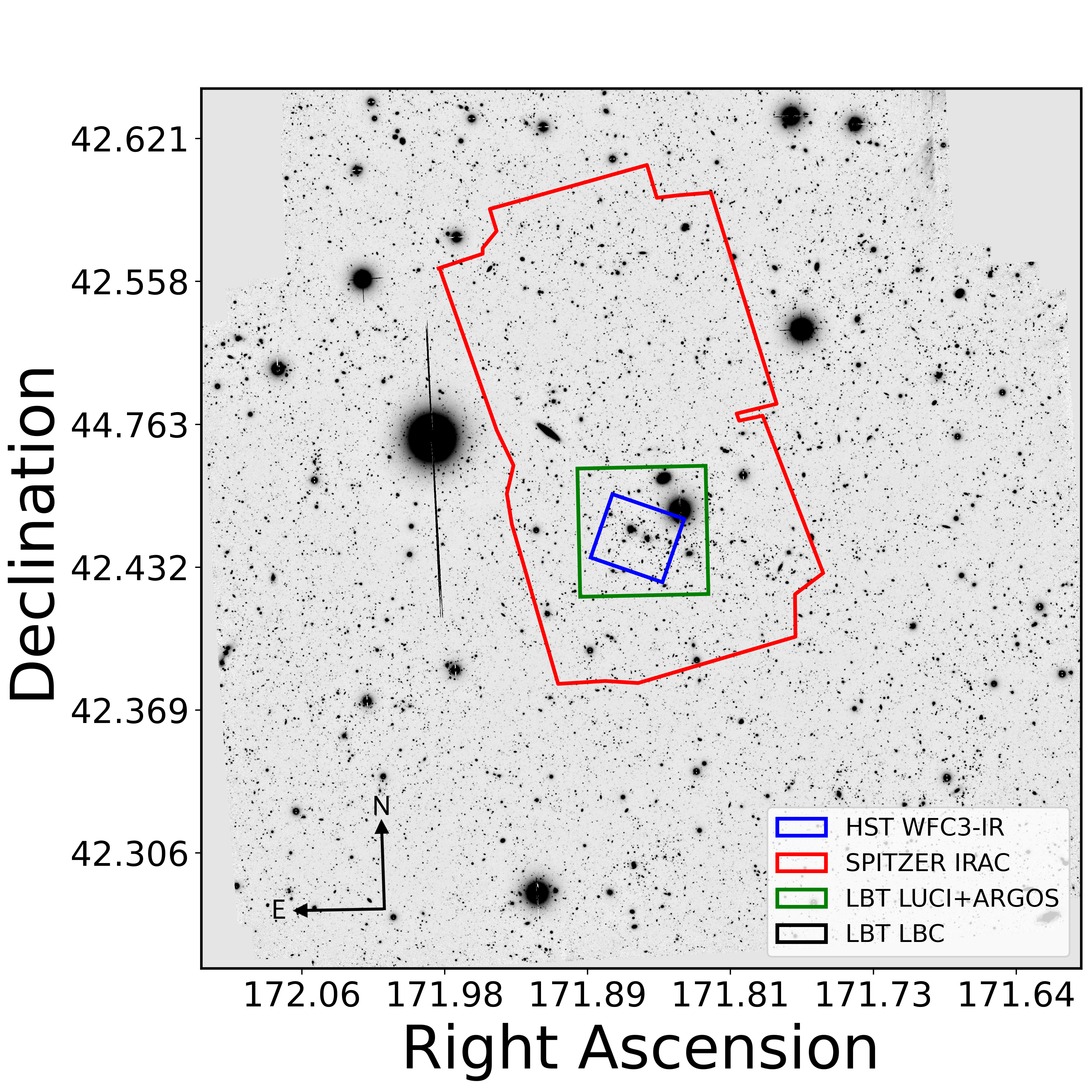
Figure 1: Footprint of the four instrument mosaics which make up the 7 filters contained in this study. The LBT/LBC field-of-view is depicted by the x- and y-axes, equating to 25^′ $\times$ 27^′ (black frame). The fields-of-view covered by Spitzer/IRAC (red), LBT LUCI+ARGOS (green), and HST WFC3-IR (blue) are also depicted. The HST WFC3-IR filters limit the FOV for which photometric redshifts can be estimated to the central $\sim$2 arcminutes of the cluster, which equates to $\sim$600 kpc at the mean cluster redshift of 0.35.

Briefly, we performed initial calibrations of the bias-subtraction and flatfield corrections in the usual way. To correct for fringing, a superflat was generated by masking out the bad pixels and bright sources over subsets of contiguous science frames, median-combining them, and then dividing the superflat into the data. To compute the astrometric solution, the SCAMP software (Bertin et al., 2002; Bertin, 2006) was run through the Theli wrapper, selecting the Initial GAIA Source Catalog (IGSC) as the astrometric reference (Gaia Collaboration et al., 2016). Visuals and intermediate data products were produced as sanity checks to ensure that the dither pattern was recognized, the distortion pattern was measured, and the positional residuals were low and evenly distributed about zero. Following the initial frame calibration and registration, the background was modeled using Theli’s internal pipeline. Finally, the individual frames were co-added using SWarp (Bertin, 2010) run from within the Theli GUI. Figure 1 depicts the $i$-band image of the full 25^′ $\times$ 27^′ field-of-view (FOV) of LBT/LBC (outermost black frame), which reaches 3-$\sigma$ limiting magnitudes of $g_{AB}$ = 25.42 mag, and $i_{AB}$ = 24.67 mag.

To test the absolute $gi$ LBT/LBC photometry, the positions of the sources in the central 5 $\times$ 5 arcmin FOV were matched with their counterparts in the Sloan Digital Sky Survey (SDSS) DR16 catalog (Ahumada et al., 2020). On computing the magnitude differences of $g_{SDSS}-g_{LBC}$ and $i_{SDSS}-i_{LBC}$, and making a 3-$\sigma$ clip to remove outliers, we measure mean offsets of 0.37 and 0.29 mag for $g$ and $i$, respectively. This means that our LBT/LBC photometry was systematically brighter by those amounts. Figure 2 shows the magnitude difference histograms following the zeropoint offset correction that minimizes the mean difference to zero. The adopted photometric zeropoints are recorded in Table 1, and are used to extract the photometry. In sum, these images are deep, making them valuable for this study, and giving them leverage as veto bands for the planned high-redshift galaxy searches using Prime Extragalactic Areas for Reionization and Lensing Science (PEARLS; program #1176).

Table 1: The Sample: Observing Details

Filtera	Exp. (s)	$m_{lim}^{b}$	FWHM (′′)c	$m_{zp}^{d}$
$g$	4090	25.42	1.37	27.57 + 0.25
$i$	2600	24.67	1.07	28.31 + 0.32
$F110W$	2664	28.94	0.13	26.82 + 0.05
$F160W$	2556	27.97	0.15	25.95 + 0.00
$K$	120	24.07	0.29	25.74 + 0.18
Ch1[3.6]	1200	23.31	1.95	21.59 + 0.21
Ch2[4.5]	1200	23.33	2.02	21.58 + 0.14

The LBT Advanced Rayleigh Ground layer adaptive Optics System (ARGOS; Rabien et al. (2019)) operates through the existing LUCI instrumentation. LUCI+ARGOS corrects the atmosphere for ground-layer distortions via multiple artificial stars which are projected by laser beams mounted on each of the two 8.4 m apertures. Observations of the G165 field were obtained in the $K$-band in 2016 December 16 (2016B; PI: Frye). We acquired the LUCI+ARGOS imaging in monocular mode with native plate scale of 0.12^′′ pixel^-1. The observing details are recorded in Table 1, and the image reduction are presented in F19 and in Rabien et al. (2019). In the reduced images, we measure a value for the point source FWHM $\approx$ 0.29^′′. This angular resolution is comparable to HST within a factor of two, effectively extending the red wavelength reach of HST. We performed our own photometry on these data, using the instrumental zeropoint AB magnitude drawn from Table 9 of the LBT LUCI users manual.

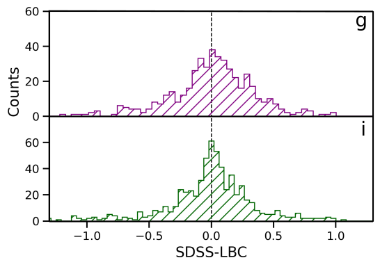
Figure 2: Histogram of the SDSS photometry relative to our LBT/LBC photometry. We measure mean systematic offsets within the central 5^′ x 5^′ FOV of 0.37 and 0.29 mag in $g$- and $i$-bands, respectively. The magnitude difference histograms reflect the distributions after the correction has already been made. The corrected photometric zeropoints are recorded in Table 1. We refer also to §4.6.1 for details regarding an independent test of the zeropoints.

2.1.2 Hubble Space Telescope

Observations were obtained between 2015 December and 2016 July as a part of an HST WFC3-IR program (Cy23, GO-14223, PI: Frye). Exposures were taken in the $F110W$ and $F160W$ passbands (0.13^′′ pixel^-1), reaching 3-$\sigma$ point source limiting magnitudes of 28.94 and 27.97 AB mag, respectively. Details of the observations are summarized in Table 1, and a description of the calibration and image reductions can be found in F19. WFC3-IR $F160W$ is used as the detection image or High Resolution Image (HRI) for the matched aperture photometry performed in this study.

2.1.3 Spitzer

Spitzer Infrared Camera (IRAC) 3.6 and 4.5 $\mu$m imaging was taken in 2016 as a part of a larger program (Cy13, GO-13024, PI: Yan). The observing details can be found in Table 1, and the image reduction is described elsewhere (Griffiths et al., 2018). Images of the central region, and of the multiple images of the Dusty Star Forming Galaxy (DSFG) Arc 1 that is singularly detected using the Planck telescope, appear in F19. The Spitzer data have a native plate scale of 1.22^′′ pixel^-1 that is larger than the other filters used in this study. Yet these data are important for their role in settling photometric redshift ambiguities, particularly for distinguishing between natural continuum breaks such as the 4000 Å and Balmer breaks and lower redshift sources that are intrinsically dusty. We extract the photometry for the O/IR imaging by the T-PHOT method, as is described in §4.5.

2.2 VLA and LOFAR

Karl G. Jansky Very Large Array (VLA) 6 GHz imaging was acquired as part of a larger program (18A-399, PI: P. Kamieneski). Details of the image reductions will appear in an upcoming paper (Kamieneski et al. 2022, in preparation). Briefly, the G165 field was observed with C-band ($4-8$ GHz) with full polarization in a 3-hour track to improve $uv$-coverage, amounting to a total of 1.5 hours of on-source integration time. Baselines for this A-configuration observation ranged from 0.68 km to 36.4 km, resulting in a natural-weighted synthesized beam size of $0.65\arcsec\times 0.37\arcsec$ at a position angle of 72^∘ and a maximum recoverable scale of $8.9\arcsec$. The sensitivity is measured to be 2.7 $\mu$Jy beam^-1 across the approximately 4 GHz of effective bandwidth. Data calibration and reduction were performed with the Common Astronomy Software Applications (CASA) package (McMullin et al., 2007), and the VLA Calibration pipeline. The radio maps uncover two head-tail radio galaxies which are discussed in §8.2.

Low Frequency Array (LOFAR) radio observations were acquired on 2016 March 22 through a single object request (PIs: Lehnert, Dole & Frye), as part of the Two-meter Sky Survey (LoTSS; Shimwell et al., 2017, 2019). The FITS image was delivered on 2019 February 19, following on-site calibration by the Default Preprocessing Pipeline (DPPP; van Diepen et al., 2018). These low-frequency (120$-$168 MHz) data have a typical angaular resolution of $\sim$6^′′ and a sensitivity of $\sim$100 $\mu$Jy beam^-1. Large-scale radio emission is detected over a $\sim$500 kpc scale that potentially arises from radio jets and/or electrons which are re-energized as a consequence of large-scale turbulence.

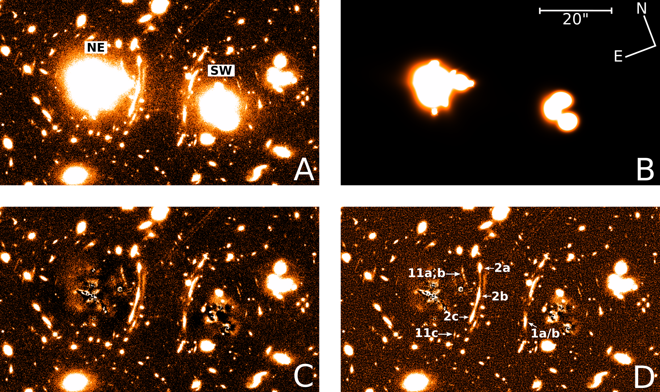
Figure 3: Preparation of the HRI $F160W$, as described in §3. The panels represent each stage in order of operation: (Panel A) the original reduced $F160W$ image; (Panel B) the best fit Galfit models for the 13 central galaxies and ICL discussed in §3.1 and §3.2; (Panel C) the model subtracted $F160W$ image; (Panel D) the median corrected image, which significantly flattens the residual over-subtractions discussed in §3.3. The two sides of the cluster are referred to as the northeast (NE) and southwest (SW) components, as labelled. The image sets for which we report new photometric redshift estimates are also labeled and discussed separately in §4.6.2.

2.3 Spectroscopy

New multi-slit spectroscopy was obtained on 2019 February 8 using MMT/Binospec (PI: Frye, 2019A). To maximize the redshift search space, we selected the 270 lines mm^-1 grating, which covers a wavelength range of 5500 Å about the central wavelength of each slitlet at a dispersion of 1.3 Å pix^-1. We observed the central region of the G165 cluster in a single pointing consisting of two 8^′ $\times$ 15^′ fields at a separation of 3.2 arcminutes. A total of 88 bright ($i_{AB}$ $<$ 22) galaxies populated the slitmasks. The observations were composed of 6 $\times$ 1200 s exposures, and were acquired under relatively-stable seeing conditions of $\sim$1^′′ as measured off of isolated sky lines. This result sufficed for our science goal to measure spectroscopic redshifts given the 1^′′ slitwidth and the relatively-bright magnitudes of our targets. The data were reduced using the observatory pipeline, which performed the bias correction, flat-fielding, wavelength calibration, relative flux correction, co-addition, and extraction to 1D spectra. Although redshift-fitting software was available, we opted to measure the spectroscopic redshifts of the coadded 1D spectroscopy in IDL by way of our own software. The SPEC task has a library of spectroscopic features and a reference sky spectrum extracted from the pre-sky-subtracted data, and is described elsewhere (Frye et al., 2012, and references therein). Our catalog contains the secure spectroscopic redshifts for 86 of 88 sources. Of these, we find eight new galaxies which meet our criteria for cluster membership as defined in §6.2.

3 Image Preparation for Photometry of the HRI

3.1 Motivation

Limited to a 7-band filter suite, the photometry in each band is impactful for making satisfactory SED fits. We perform the multiband photometry using the prior-based software package T-PHOT, which is designed to do photometry across images drawn from different observing facilities and/or instrument modes, and to different field depths. A single HRI is designated with which to extract the master object catalog. To retain its information, priors on object morphology are derived from the HRI which are then enforced onto the images in the six other filters or Low Resolution Images (LRIs).

T-PHOT enlists two types of priors to generate a model of the LRI. The ‘real’ prior consists of cutouts from the HRI which are informed by the photometry, and is especially sensitive to background sources of light. To approximate this background, we carefully model both the ICL and the bright galaxy light components, where the latter component becomes the ‘analytic’ prior. Our approach follows closely the methods of the ASTRODEEP catalogs of the Frontier clusters (Merlin et al., 2016; Castellano et al., 2016), and we refer also to the companion flowchart in (Merlin et al., 2016, their Figure 1). Once obtained, the background model is refined by an iterative process, and then subtracted off of the HRI. The background-subtracted HRI is further corrected for any residual light, as is described below.

3.2 Galfit Setup

The background modeling algorithms used in this study make extensive use of the Galfit tool (version 3; Peng et al., 2010). Galfit operates on an input science image in units of counts, and a sigma image, which is a map of the standard deviation of the science image. The sigma image can be generated externally, by using the weight files outputted from the HST MultiDrizzle task following Casertano et al. (2000), and also internally by inputting the values from the image headers into Galfit. To test the relative merits, we ran Galfit on a “sky” object consisting of a rectangular isolated region of sky. We found the reduced $\chi^{2}$ to favor the internal approach, as the weight images underestimated the actual noise in the complex cluster scene, and adopt this method for generating the input sigma image for all of our Galfit modeling.

3.3 Initial Background Model Fits

The background consists of two components: (1) the intracluster light (ICL), and (2) the light from individual galaxies. We constructed an initial model for the ICL component by masking out all pixels in the HRI greater than $8\sigma_{sky}$, where $\sigma_{sky}$ is estimated by sampling the sky in three small and statistically significant patches of the image separated from known sources. We then select the modified Ferrer profile included in Galfit, which is prescribed in Merlin et al. (2016) and Giallongo et al. (2014) due to its relatively flat core and freedom to change the sharpness of its truncation when compared to similar Sérsic profiles. As expected, a combination of two modified Ferrer profiles provided the best fit to the two light peaks visible in the data (Panel A of Figure 3). We note that while parameters like bending modes, diskiness/boxiness, and other profiles (e. g., Sérsic) were tried, they did not improve the results and hence were discarded. The best-fit ICL model was then subtracted from the original image.

Our model for the cluster galaxy light contains the brightest cluster member in the field, the Brightest Cluster Galaxy (BCG), and five other dominant central cluster members or Large Red Galaxies (LRGs) and their nearest satellites, to constitute a set of 13 galaxies. The inclusion of the satellite galaxies enables a better fit to the galaxy light by our Galfit approach. These bright galaxies typically require more than one Galfit profile to best model their overall brightness profile. Simultaneously fitting many Galfit profiles, however, can give rise to degenerate solutions, ultimately preventing Galfit from converging to a best-fit solution. We instead adopt an iterative approach, beginning with only a single Sérsic profile. For this initial fit, we make use of the software package Galapagos, which contains the desired functionality by performing separate Galfit fits for all objects at the positions given in SExtractor (Barden et al., 2012). We found that using a single profile per galaxy in this initial fitting stage helps to prevent degeneracies in the subsequent two-profile refinement fitting stage, as is described below.

We iterate on the initial galaxy light model by introducing an additional Sérsic profile, such that each galaxy model is made up of two Sérsic profiles. Following the prescription of Merlin et al. (2016), we use the best fit parameters of the initial models to place constraints on the parameters of the refinement model. Some individual galaxies required even further refinement, with errors in the position angle and/or axis ratios evident by a visual comparison between the model and image. We tighten up the fitting constraints on an object by object basis, iterating as needed until a solution is reached that, upon visual inspection, produces reasonably flat residuals.

We then return to the ICL model and iterate on it by applying the results of the revised galaxy light model as a fixed component in Galfit, while both ICL Ferrer components from the ICL initial fit are left free. This step allows the ICL fit to be readjusted relative to the new bright galaxy model fits, thereby superseding the simple 8$\sigma$ mask that was initially enforced in §3.1. The only other constraint placed on the ICL components is a position center good to $\pm 1$ pix from the initial value in each coordinate. The results did not vary much from the initial ICL fit, providing a check on the quality of our overall fit. The resulting image depicting the combined background light appears in Panel B of Figure 3.

3.4 Residual Corrections

Subtracting the background image from the data leaves regions of negative flux. To alleviate the impact of these image residuals, we follow the prescription in Merlin et al. (2016). The procedure is to run SExtractor on the sky surrounding each bright galaxy to estimate the sky RMS, $\sigma_{SE}$. Next, the image is median-filtered using the PyRAF task median, imposing a 1^′′ x 1^′′ window and excluding all pixels $>$ 1$\sigma_{SE}$ and neighboring pixels. Finally, the median-filtered image is subtracted from the residual of the original image. The resulting image has the expected flatter background adequate for doing photometry (panel D of Figure 3). Since the photon noise is retained in the residual image, and the Galfit models themselves contain no noise, we do not find it necessary to adjust the $F160W$ RMS map in the subtracted image.

4 Photometry

4.1 Overview

We describe below our measurement of the photometry in the HST filters using SExtractor, and in the other LRIs using T-PHOT. To achieve a more realistic model for each LRI, T-PHOT is informed by the two different priors described in §3.1. In what follows, the real prior is obtained from the SExtractor catalog (§4.2), and the analytical prior is taken from the bright galaxy models (§3.2). The two priors are stitched together into a single 2D image which is referred to as a collage. This collage is subsequently degraded to match the PSF, and then scaled to match the flux of each LRI. This final step in the process yields the photometry for each LRI.

4.2 Object Detection

The HST WFC3-IR $F160W$ image is our object detection reference, or HRI. We perform the photometry using SExtractor (Bertin & Arnouts, 1996) by implementing a two-step HOT+COLD method according to the prescription in Galametz et al. (2013). In this prescription, the COLD parameter set is tuned to the detection of bright, extended galaxies, while the HOT parameter set is optimized to detect the fainter galaxies not included in the preceding COLD mode run. We choose to match the parameters of Galametz et al. (2013) rather than Merlin et al. (2016) given the limited depth of our HRI, as the HOT mode run in Merlin et al. (2016) is significantly more aggressive than Galametz et al. (2013), producing many more spurious sources without additional true sources in our case.

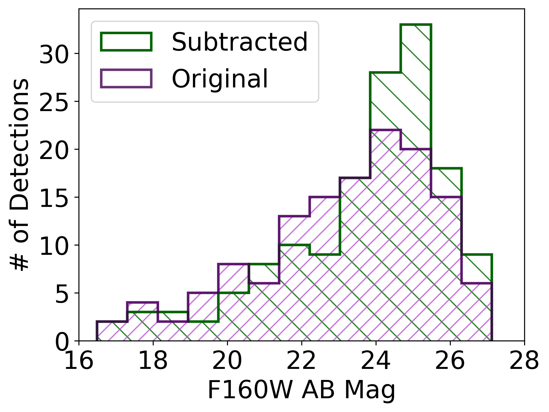
Figure 4: Object counts in the central cluster region as a function of $F160W$ AB mag (purple) relative to object counts extracted from the background-subtracted image (green). We delineate the central region by a 72^′′ $\times$  24^′′ rectangle that runs along the long-axis of the cluster, covering the central LRGs on both the NE and SW sides of the cluster (Panel A of Figure 3). We detect 147 objects in the processed image, equating to a 10% increase from the 135 objects detected in the original image using the same SExtractor parameters. We measure more accurate photometry of central objects by their reduced contamination from the background light, and detect fainter objects, thereby pushing detections to fainter limiting magnitudes. We refer to Figure 5 for specific examples.

The two catalogs and their SExtractor segmentation maps are combined non-redundantly following the methods of Galapagos. The COLD mode sources are all catalogued, and only HOT mode sources outside the Kron ellipses of the COLD run are accepted. The combined catalog contained 1228 sources. We clean this list by hand to remove artifacts such as edge effects, diffraction spikes, and residuals from the BCG subtraction. The final detection catalog contains 964+13 sources, with an average aperture Kron ellipse radius of 0.2^′′. The ‘+13’ here refers to the initial 13 bright sources in the image which are separately modeled by Galfit, and are subtracted prior to detection with the HOT+COLD method. We find the bright galaxy light and ICL subtraction described in §3 yields larger numbers of faint objects in the central region of the cluster

as is demonstrated in Figure 4. The photometry of faint objects is also more accurately recovered,

as depicted in Figure 5. This HRI photometric catalog and its accompanying segmentation map serve as the inputs for the multi-band photometry in T-PHOT. However, the default SExtractor segmentation map can cause inaccuracies in T-PHOT photometry for smaller sources (Galametz et al., 2013). To complete its setup, we had to modify the segmentation map of the HRI slightly by scaling the source area in the map with the dilate software (De Santis et al., 2007).

4.3 Image Alignment and PSF Constructions

PSFs need to be constructed for each LRI to prepare the images for simultaneous photometry. We start by aligning the images in each filter to the HRI in a two step process using the astropy package reproject and astroalign tasks. We find astroalign outperforms reproject in producing astrometrically precise image alignment, but fails when images are significantly misaligned. Hence, we first apply reproject, which transforms images to the same orientation and pixel scale based on the WCS header information. We then follow up on this step by applying the astroalign task in order to triangulate the source centroid positions and to calculate a revised value for the reprojection according to Beroiz et al. (2020). We describe below the process of obtaining a good sampling of the PSF for each of the seven bands.

For the LBT/LBC $gi$ filters, we extract an initial catalog of stars using the DAOStarFinder subroutine according to Stetson (1987). We then visually inspect the output star list and cull out by hand a set of 100 suitable (well isolated and unsaturated) stars. Cutouts centered on each star are extracted and are subsequently median-subtracted and normalized to lessen the impact from image contamination. Finally, the stellar cutouts are stacked into a single oversampled PSF using the EPSFBuilder function from the photutils python package.

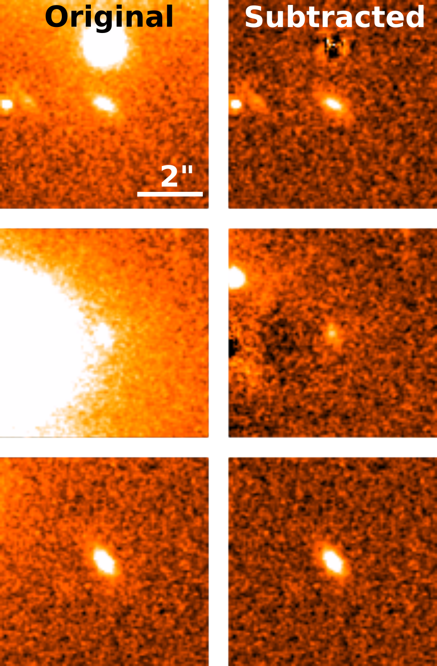
Figure 5: Images centered on three of the 964 galaxies detected in the HRI (HST WFC3-IR $F160W$) in the initial image (left-hand side, drawn from Panel A in Figure 3), and upon subtraction of the background (right-hand side, drawn from Panel D in Figure 3). In each example, the photometry of the background-subtracted image is fainter by at least 0.5 AB mag as a result of removing the contaminating light. A second effect of the background-subtraction is to enable detection of fainter sources because the noise level decreases. Both effects operate in the direction of increasing number counts in the fainter magnitude bins (Figure 4).

For HST WFC3-IR $F110W$ and $F160W$, we adopt the PSFs provided by STScI. These nine PSFs sample the profiles in different locations across the detector. We average all nine of them together to produce a single representative PSF. One averaged PSF is taken for each exposure that makes up the coadded image, and the PSF is rotated as needed, based on the WCS image header information. The individual exposure PSFs are subsequently averaged together and weighted by the exposure time to yield the PSF for the coadded image.

For the LUCI+ARGOS $K$-band image, the 4^′ $\times$ 4^′ FOV lacked well-isolated, unsaturated stars, and only contained a handful of stars in total. While we found the astropy stacking method to produce a reasonable-looking PSF by-eye, we obtained a PSF that produced flatter residuals in the T-PHOT stage by fitting a 2D Gaussian to crowded but unsaturated stars in the field. The resulting Gaussian has a FWHM of $0.29^{\prime\prime}$, consistent with previous results (F19).

For the Spitzer IRAC image PSFs, we took two different approaches to build the PSF. First, we stacked the PSFs of isolated stars similar to the approach outlined above for the LBT/LBC $gi$ images. Second, we tried using a set of 25 analytic PSFs supplied by the Spitzer Science Team, which are each rendered onto a 5 $\times$ 5 pixel grid across the detector. For each individual exposure that makes up the IRAC coadded image, we interpolated over this PSF suite to generate the one that most closely corresponds to the location of each object in our catalog. Each PSF is then rotated according the orientation of its exposure relative to the coadded image. All of the rotated PSFs are then averaged together, and weighted by the exposure time. The product is an individual analytical PSF for each object in the catalog. We ultimately adopt the stacking method approach for obtaining the PSFs, as it produced noticeably flatter residuals in the T-PHOT stage. At the same time we acknowledge that the analytical model method has been demonstrated as preferable in other studies (Merlin et al., 2016, 2021; Pagul et al., 2021).

4.4 Photometry starting with the $F160W$ and $F110W$ filters

The $F110W$ image was prepared by the same process as described in §3 for the HRI. We start by applying the final Galfit models for $F160W$ as the initial models for $F110W$ and fit for all objects simultaneously, including the ICL. The resulting models are subtracted from the $F110W$ image and then undergo the same median subtraction process applied to the $F160W$ band. $F110W$ is then convolved with a matching kernel to the PSF of $F160W$. The matching kernel, $K$, is created by taking the ratio of the PSF of each image as per the convolution theorem, which states that the integral of two quantities is equivalent to their multiplication in Fourier space. Hence, we can write

$$\text{PSF}_{2}=K\bigotimes\text{PSF}_{1}$$

where PSF₁ is the $F110W$ PSF and PSF₂ is the $F160W$ PSF. By the convolution theorem

$$\mathcal{F}(\text{PSF}_{2})=\mathcal{F}(K)*\mathcal{F}(\text{PSF}_{1})$$

$$K=\mathcal{F}^{-1}\left(\frac{\mathcal{F}(\text{PSF}_{2})}{\mathcal{F}(\text{PSF}_{1})}\right)$$

as desired. We apply a simple Cosine window function prior to convolution to eliminate any spurious modes picked up by noise. Generating a new RMS map for $F110W$ following the convolution is not straightforward, and we choose to approximate the new map with the original RMS map due to the similarity in PSF FWHM between $F110W$ and $F160W$. We then enforce the same apertures as used on the HRI via SExtractor’s dual image mode, selecting the $F160W$ image and its associated weight map for detection but the $F110W$ image and its weight map for measurements. This forced object catalog makes image registration more straightforward and alleviates some of the issues relating to image blending, yielding more accurate measured fluxes across both images. We cite the $F160W$ magnitude as the AUTO magnitude, which is measured selecting the Kron-like elliptical aperture, and we calculate $F110W$ magnitude by computing the difference in isophotal aperture magnitudes between the $F160W$ and $F110W$ bands added to the $F160W$ AUTO magnitude. We justify the isophotal selection aperture in this case because it is better at measuring colors, while the AUTO aperture better measures the total fluxes (Coe et al., 2006). Magnitude errors are derived using SExtractor, with the slightly larger $F110W$ errors resulting from the propagation of errors of each quantity used.

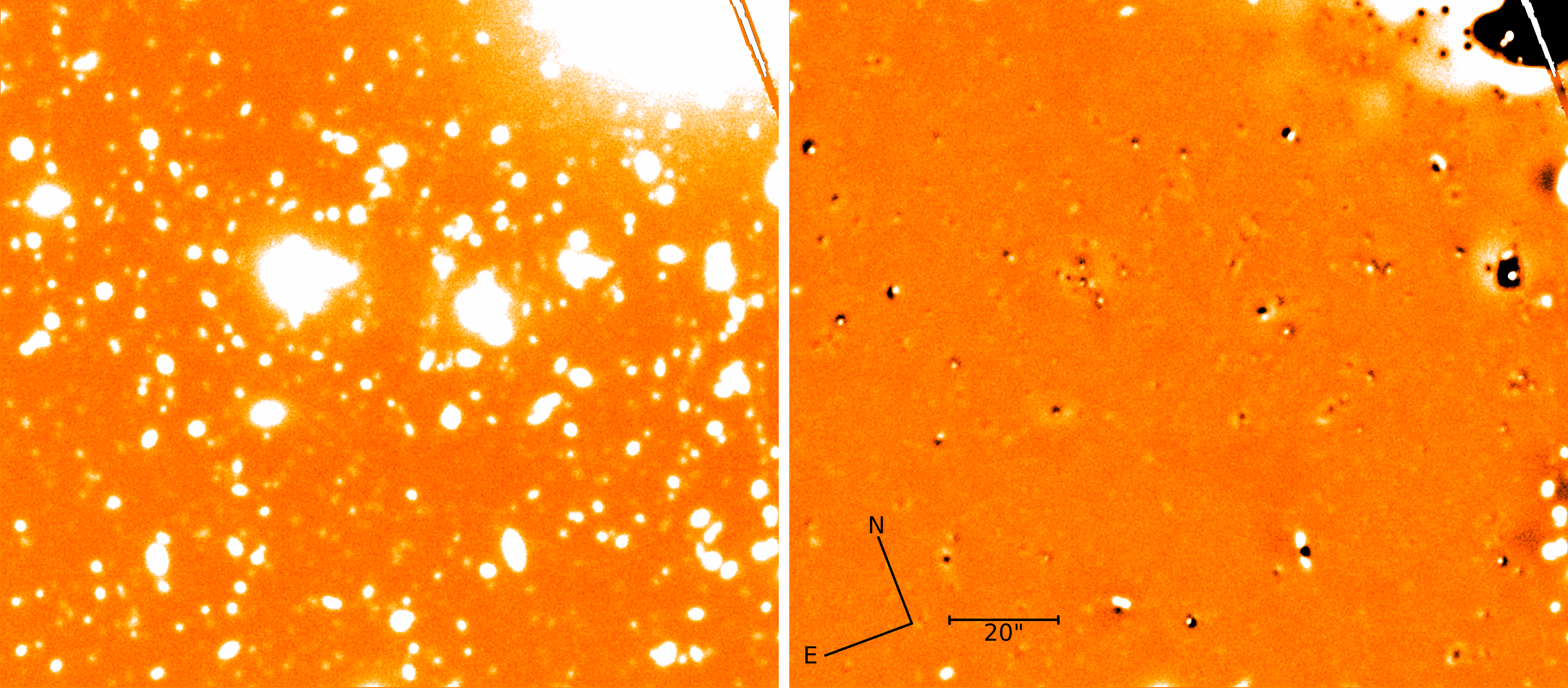
Figure 6: Quality check on the T-PHOT photometry for the LBT/LBC g-band LRI (left panel). T-PHOT creates a photometric collage from the HRI ($F160W$) and scales it to minimize the residual between the collage and the LRI. The residual is flat (right panel), indicating a good fit of the image priors to the data across the field (§4.5).

4.5 Photometry incorporating the other LRIs

The LBT/LBC $gi$, LBT/LUCI $K$, and Spitzer IRAC $Ch1$ and $Ch2$ bands all have larger PSF sizes relative to the HST images, making image blending more of a problem. We perform the multi-band photometry using T-PHOT in a similar way across all five of these LRIs. The HRI ($F160W$) catalog supplies the positions and fluxes of cutouts for the real prior, while the HRI Galfit models are applied as the analytical prior. Both sets of priors are held fixed in all T-PHOT runs across all LRIs. The only difference between these T-PHOT runs is the required matching kernel for degrading the HRI cutouts to the LRI PSF, which we already derived in §4.3. For $giK$, the matching kernel is constructed using the filter’s data-derived PSF and the analytical $F160W$ PSF through the Fourier methods explained in §4.4. For the Spitzer/IRAC channels, the PSF itself is applied as the matching kernel owing to its large profile compared to $F160W$ (Galametz et al., 2013).

We initiated a series of two T-PHOT runs on the 5-filter image stack. T-PHOT photometry is especially sensitive to the LRI background, hence the purpose of the first T-PHOT run is to estimate the background of the LRI using the built-in option for local background estimation. Flat background object counterparts are assigned to each object in the input catalog. All objects are fit simultaneously, returning the 2D image collage as outlined in §4.1. We modify this collage to only retain the fitted flat background objects, yielding the background model. This model is subsequently smoothed using a 2D Gaussian kernel to produce a relatively smooth approximation of the image background. This background model is subtracted from the image to yield the final background-subtracted image.

To produce the multi-band photometry, we perform a second T-PHOT run on the background-subtracted images of the 5-filter suite. As a gauge of the quality of this run, the original LRI is compared to the LRI with the T-PHOT collage subtracted from it. A flat residual image, such as the one shown in Figure 6 for the $g$-band, indicates a good fit of the image priors to the data across the field. This procedure allows for iterative modifications to the image priors until a satisfactory residual is obtained.

Each T-PHOT run returns a covariance index that correlates with the quality of the fit. The covariance index is sensitive to the effects of crowding on the T-PHOT fit, such that covariance indices greater than unity suggest a high degree of degeneracy between the fit photometry of neighboring objects. We cite photometric errors according to the output from T-PHOT. We stress that these uncertainties are statistical relative to the input RMS map, and do not include systematic errors, such as artifacts introduced by the PSF estimation, or any remaining non-uniform background in the $F160W$ image cutouts. Systematics are broadly accounted for in the photometric redshift estimation by enforcing a floor minimum uncertainty level for the input photometric measurements amounting to 0.05 mag for the $F110W$, $F160W$, and $K$ filters, and 0.1 mag for the $gi$ and IRAC filters as in Merlin et al. (2016), Bradac et al. (2019) and Pagul et al. (2021).

4.6 Preparation for Photometric Redshift Estimation

We estimate photometric redshifts with the Bayesian Photometric Redshift (BPZ) software package (Benítez, 2000; Benítez et al., 2004; Coe et al., 2006). BPZ fits photometric measurements to SEDs of different galaxy types using Bayesian inference. Crucially, the Bayesian approach utilizes assumed priors on $i$-band brightness and galaxy type such that only the SEDs which best represent the input photometry are fit to the data. BPZ produces a best fit redshift and a galaxy type by interpolating over SED templates provided by Coleman et al. (1980), Kinney et al. (1996), and Bruzual & Charlot (2003). In preparation to doing accurate photometric redshift estimation with BPZ, we also make adjustments to the photometric zeropoints and apertures.

4.6.1 Zeropoint Correction

We initially trained BPZ on a subset of 20 objects which also have spectroscopic redshifts. This involved fixing the object redshift to the spectroscopic redshift and then enforcing BPZ to fit the SEDs by only allowing the galaxy type to vary. In turn the BPZ code outputs suggestions of any zeropoint magnitude offsets. This is an iterative process in which an offset is computed, and then the code is rerun, until the suggested offset approaches zero.

We found the magnitude offsets to be small or zero in most bands. We did, however, notice non-negligible suggested offsets of $\sim 0.35$ and $\sim 0.25$ magnitudes in LBT $g_{AB}$ and $i_{AB}$, respectively. To explore this difference, a second test was conducted comparing the photometry in the central the central 5 $\times$ 5 arcmin FOV with SDSS. We refer to §2.1.1 for details. Somewhat reassuringly, we obtain a similar zeropoint offset by both approaches. We opted to apply the offsets measured via the SDSS comparison for our photometry. The revised values for the zeropoint magnitudes are reported in Table 1.

Our BPZ calibration also motivated small zeropoint corrections in the IRAC images of 0.21 and 0.14 for Ch 1 and Ch 2, respectively. On further inspection, we confirmed that residuals from T-PHOT were generally more negative than the sky in those bands. We believe this is due to the unique structure and large width of the IRAC PSF. At the same time, systematic offsets in magnitude are not uncommon. For example, in one study of the HFF clusters, a minor IRAC offset was also reported of a similar degree but in the opposite direction, potentially owing to their analytical-style approach to estimate the PSF rather than our data-driven one as described in §4.3 (Pagul et al., 2021).

On applying all the zeropoint corrections to the data, the BPZ code is re-run with the full photometric catalog, freely and without any fixed redshifts, to create the photometric redshift catalog. In doing so, we impose a few criteria to ensure a valid measurement of the photometry. First, the photometry of objects whose ratios of flux to flux error are less than the measured image signal-to-noise ratio are classified as non-detections and are removed. We also throw out candidate detections for which the flux error is negative or unreasonably large, or the covariance index output by T-PHOT is larger than unity.

4.6.2 Custom Apertures on Arcs

The extraction apertures were tailored for the three sets of image multiplicities for which we achieve quality photometric redshift estimation: Arcs 1a/b, Arcs 11a,b, and Arcs 2a,c (Panel D of Figure 3). The infrared images of Arc 1a/b consist of two blue knots and a redder and more diffuse underlying component with a total angular extent of 5 arcseconds. Because the T-PHOT fitting method integrates across the image, the multi-component information gets subsequently lost. To recover the input redshift we found it necessary to place down one aperture for each knot as well one for the overall arc-shape. We refer to §4.6.2 below for details.

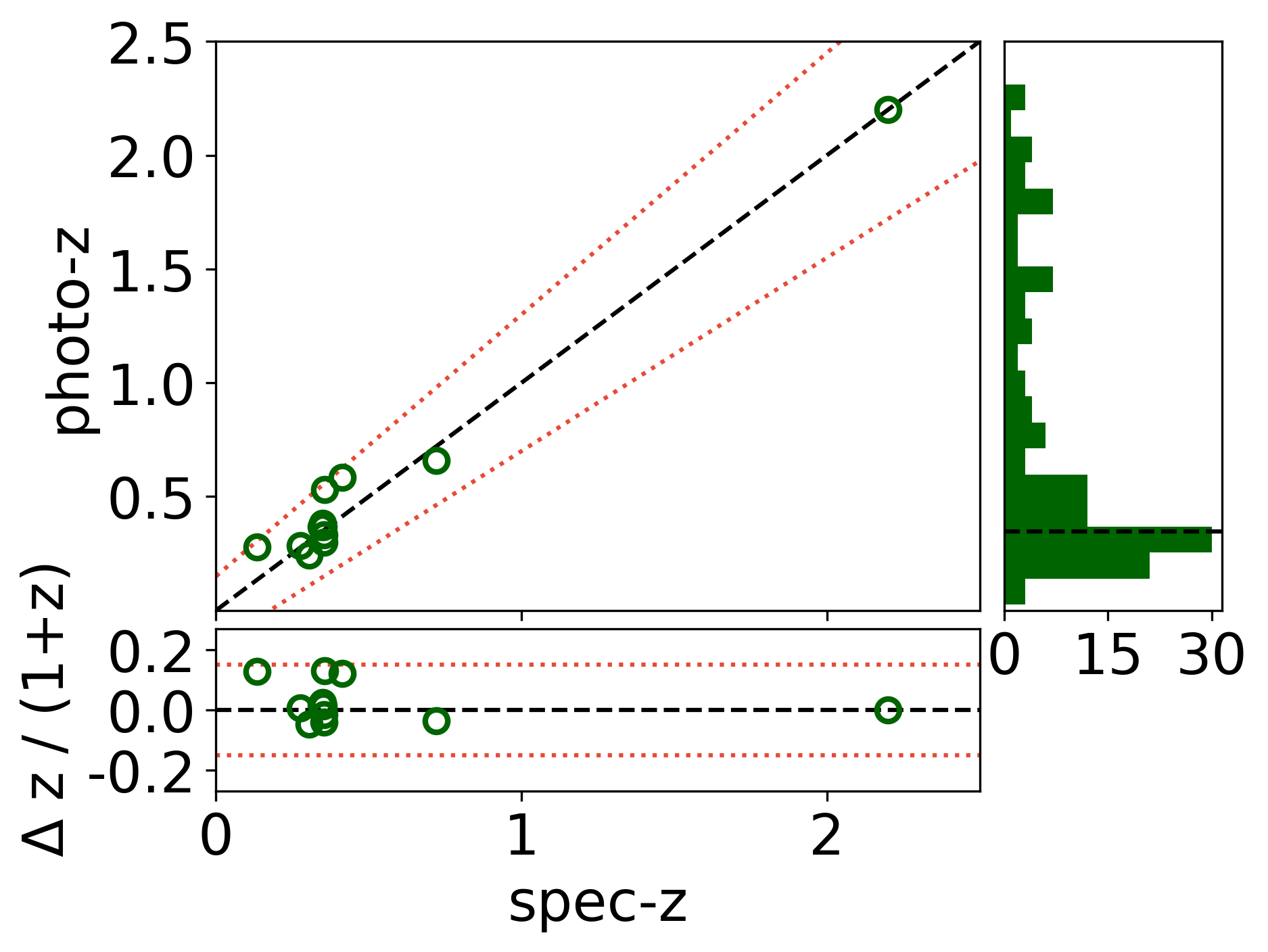
Figure 7: Comparison of the training set of galaxy redshifts with their photometric redshift estimates obtained in this study, up to $z$ = 2.5. We define a metric for the goodness-of-fit as $|\delta z|/(1+z)$ $<$ 0.15 (dashed lines) to assess the overall performance of the photometry. The histogram on the right-hand-side depicts the distribution of photometric redshifts, which peaks at the cluster redshift $z$ = 0.348 (black dashed line). We find the photometric redshift estimations to be contained within the goodness-of-fit metric for all sources.

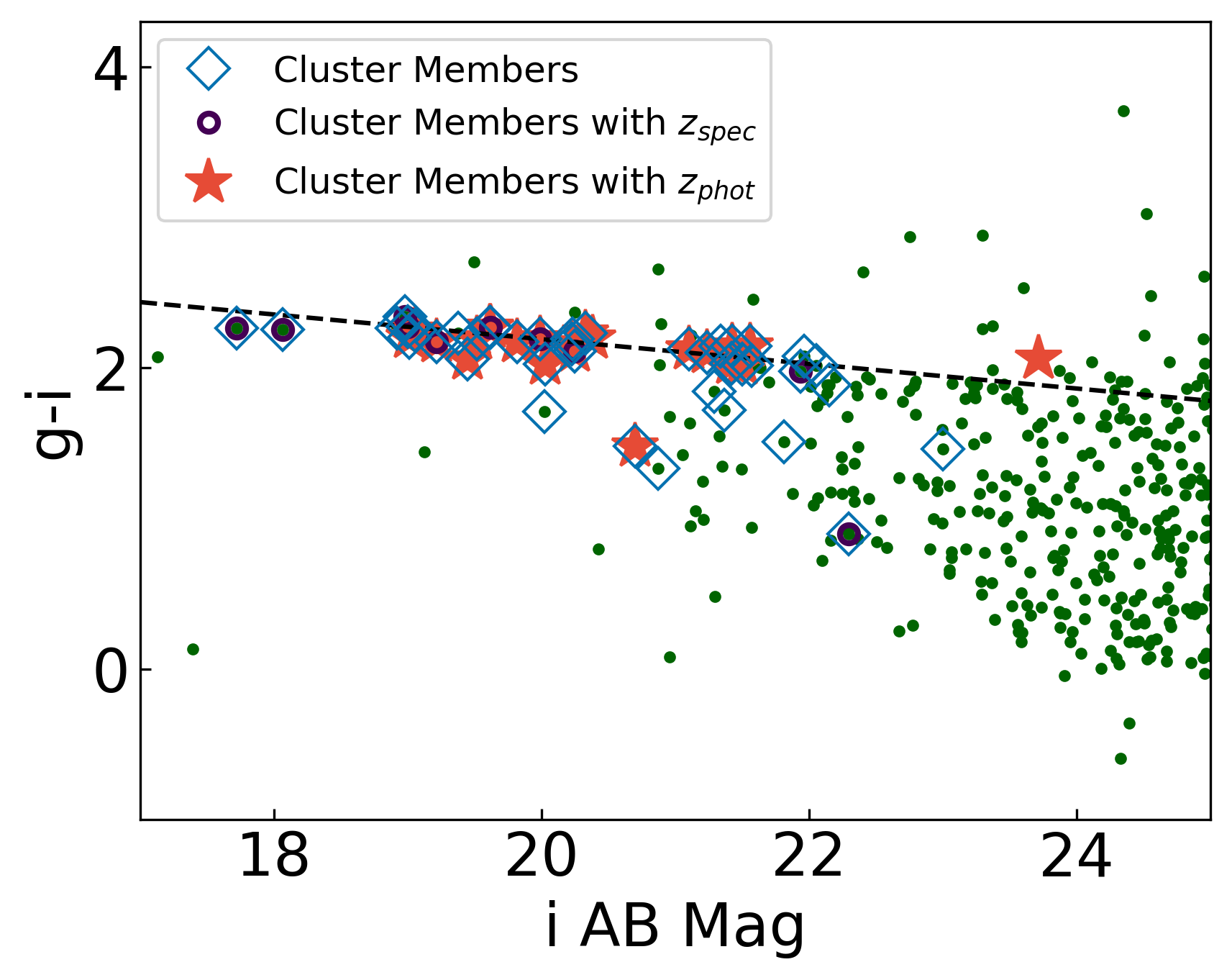
Figure 8: LBT/LBC g-i colors for T-PHOT photometry performed on objects within the HST FOV (green filled circles). The spectroscopically confirmed cluster members are depicted by the purple open circles, while the photometrically confirmed cluster members are indicated by the red stars. The cluster red sequence is depicted for reference (black dashed line), which guides the selection of cluster members applied to our lens model (blue diamonds).

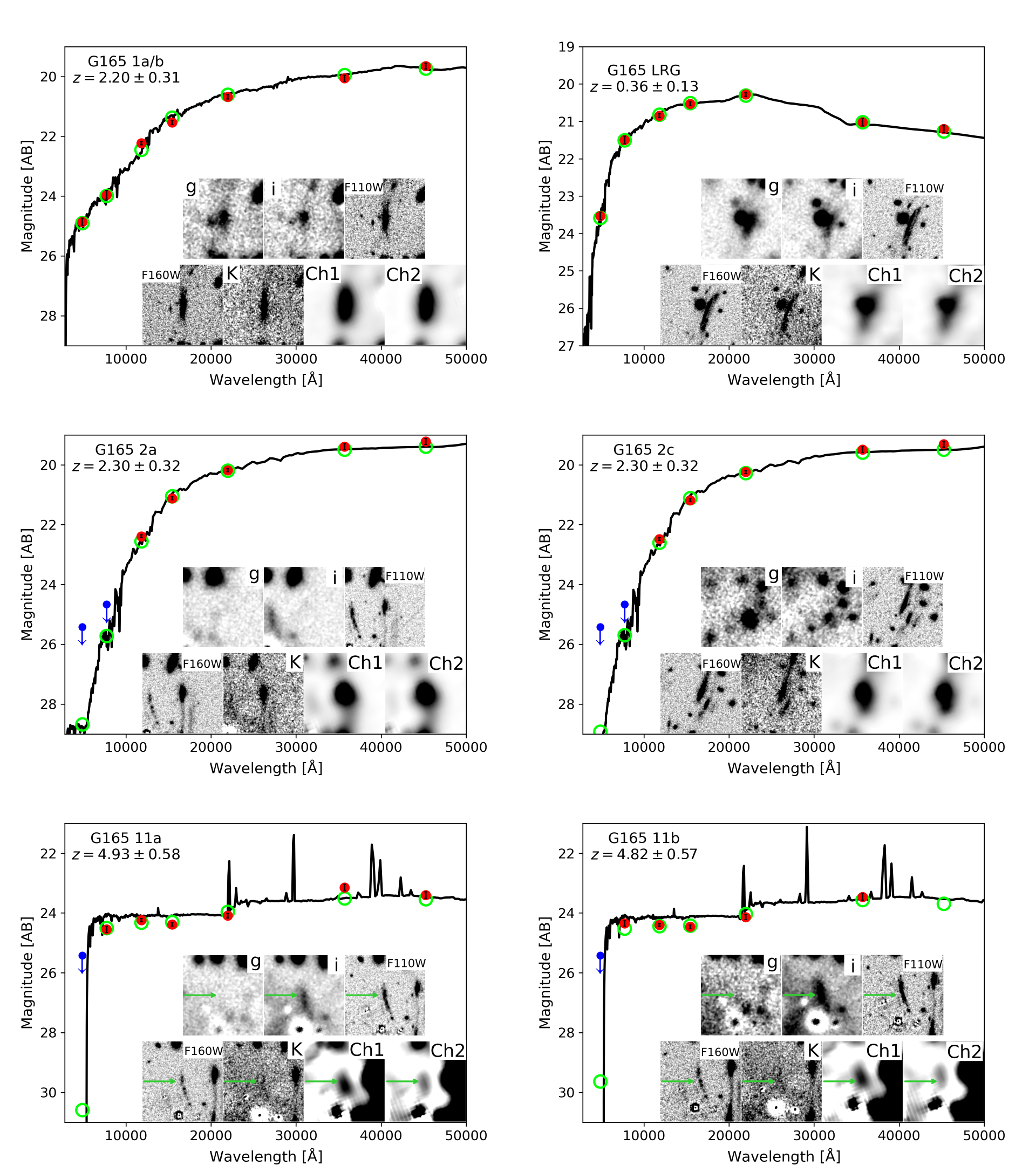
Figure 9: Best fit BPZ SEDs from SExtractor and T-PHOT photometry of Arcs 1a/b, 2a, 2c, 11a, and 11b and a typical example of a cluster LRG. The best fit SEDs (black line) interpolated from Kinney et al. (1996), Bruzual & Charlot (2003), and Coleman et al. (1980) templates satisfy our criterion for secure redshifts by returning a reduced $\chi^{2}$ $<$ 1 while using a minimum of 5 bands. SED fit quality is determined by the offset between the photometry estimated for the SED in a given filter (green circles) and the photometry measured through SExtractor and T-PHOT (red dots), as well as by satisfying the BPZ prior on the $i$-band magnitude. Drop outs (blue arrows) are reported where the measured magnitude falls below the measured 3-$\sigma$ detection limit. Image stamps of each object are shown in the insets with the filter as labeled. Photometric redshifts are obtained for these five members of three different image multiplicities, which contribute tighter constraints to the lens model.

On other image multiplicities, Arcs 11a,b consists of two bluer knots on top of a more extended, and somewhat redder, stellar continuum. For this case, we lay down four apertures, one for each of the knots. We choose not to put down an aperture over the larger arc structure because the surface brightness is low and in principle a photometric redshift can be obtained from any of the knots. This choice of a small aperture is also advantageous for minimizing background contamination. Arcs 2a and 2c are compact and bright, making them straightforward to detect using SExtractor. Given the compact morphology, further adjustments to the apertures or photometry were unnecessary.

5 Photometric Results

5.1 Photometric Catalogs

We estimate photometric redshifts for 143 galaxies, for which each galaxy is detected in at least five bands and has been confirmed to be a real source by our visual inspection. Furthermore, each SED fitting result must satisfy the condition that the modified $\chi^{2}<1$, a conservative cutoff to ensure high quality fits with BPZ introduced in Coe et al. (2006). The distribution of photometric redshifts peaks at the cluster redshift, and has a long tail extending to higher values (Figure 7). Of these, 22 objects are found to be in or near the cluster redshift, with 37 in the foreground and 84 in the background. On background objects, 42 objects are at 1 $<$ $z$ $<$ 3, with four high redshift sources at $z$ $>$ 5. The result of this study is that new optical-IR photometric redshifts are obtained for four lensed galaxy images from two image systems for which there was no previous photometric or spectroscopic values. These new values contribute tighter constraints to the lens model (§5.3, §7).

Table 2: High-z Photometry From G165 Field

ID   a	R. A.	Decl.	$z_{phot}^{b}$	$g_{AB}^{c}$	$i_{AB}^{c}$	$F110W_{AB}$	$F160W_{AB}$	$K_{AB}$	$Ch1_{AB}$	$Ch2_{AB}$
$1^{d}$	171.8113	42.47299	$2.20^{+0.31}_{-0.31}$	$23.96\pm 0.11$	$24.86\pm 0.08$	$22.23\pm 0.02$	$21.54\pm 0.05$	$20.68\pm 0.05$	$20.06\pm 0.01$	$19.65\pm 0.01$
$2^{e}$	171.81645	42.47473	$2.30^{+0.32}_{-0.32}$	$>26.1$	$>26.8$	$22.39\pm 0.00$	$21.12\pm 0.00$	$20.18\pm 0.00$	$19.39\pm 0.00$	$19.22\pm 0.00$
$3^{e}$	171.81384	42.47811	$2.30^{+0.32}_{-0.32}$	$>26.1$	$>26.8$	$22.48\pm 0.00$	$21.18\pm 0.00$	$20.24\pm 0.00$	$19.49\pm 0.00$	$19.31\pm 0.00$
$4^{f}$	171.81567	42.47835	$4.93^{+0.58}_{-0.58}$	$24.55\pm 0.01$	$>26.8$	$24.24\pm 0.01$	$24.38\pm 0.03$	$24.09\pm 0.06$	$23.15\pm 0.04$	$23.40\pm 0.03$
$5^{f}$	171.81572	42.47802	$4.82^{+0.57}_{-0.57}$	$24.35\pm 0.01$	$>26.8$	$24.40\pm 0.01$	$24.46\pm 0.03$	$24.14\pm 0.07$	$23.46\pm 0.05$	—
6	171.81575	42.47784	$5.06^{+0.59}_{-0.59}$	$25.11\pm 0.02$	$>26.8$	$24.94\pm 0.01$	$24.87\pm 0.04$	$24.61\pm 0.10$	$24.73\pm 0.10$	—
7	171.8211	42.45727	$1.86^{+0.29}_{-0.28}$	$25.67\pm 0.02$	$26.34\pm 0.02$	$25.28\pm 0.02$	$24.71\pm 0.03$	$24.69\pm 0.07$	$24.42\pm 0.04$	$24.21\pm 0.03$
8	171.84108	42.46482	$1.81^{+0.28}_{-0.55}$	$24.70\pm 0.01$	$24.98\pm 0.01$	$24.13\pm 0.01$	$23.76\pm 0.02$	$23.62\pm 0.03$	$23.46\pm 0.02$	$23.49\pm 0.01$
9	171.8184	42.45991	$1.99^{+0.48}_{-0.35}$	$27.54\pm 0.12$	$27.47\pm 0.05$	$26.88\pm 0.04$	$26.42\pm 0.10$	—	$25.98\pm 0.14$	—
10	171.83697	42.46778	$4.82^{+0.57}_{-0.57}$	$26.07\pm 0.03$	$>26.8$	$25.94\pm 0.02$	$25.78\pm 0.06$	$25.67\pm 0.15$	$24.79\pm 0.07$	$24.83\pm 0.06$
11	171.80296	42.4641	$2.00^{+0.29}_{-0.29}$	$27.30\pm 0.11$	$>26.8$	$24.04\pm 0.01$	$22.79\pm 0.01$	$22.12\pm 0.01$	$21.45\pm 0.00$	$21.34\pm 0.00$
12	171.81299	42.471	$2.05^{+0.30}_{-0.30}$	$23.91\pm 0.01$	$24.28\pm 0.00$	$23.40\pm 0.01$	$22.94\pm 0.01$	$22.66\pm 0.01$	$22.54\pm 0.01$	$22.52\pm 0.01$
13	171.81502	42.47611	$2.06^{+0.30}_{-0.30}$	$25.02\pm 0.02$	$26.60\pm 0.03$	$22.05\pm 0.00$	$20.82\pm 0.00$	$19.86\pm 0.00$	$19.13\pm 0.00$	$19.00\pm 0.00$
14	171.79628	42.46708	$1.94^{+0.29}_{-0.29}$	$23.90\pm 0.01$	$24.69\pm 0.00$	$23.67\pm 0.01$	$23.10\pm 0.01$	$23.01\pm 0.02$	$22.60\pm 0.01$	$22.57\pm 0.01$
15	171.8178	42.47324	$1.81^{+0.27}_{-0.27}$	$26.01\pm 0.03$	$28.87\pm 0.18$	$23.14\pm 0.01$	$22.26\pm 0.01$	$21.71\pm 0.01$	$21.26\pm 0.00$	$21.19\pm 0.00$
16	171.83023	42.47862	$1.80^{+0.27}_{-0.27}$	$23.56\pm 0.00$	$23.81\pm 0.00$	$23.27\pm 0.01$	$22.95\pm 0.01$	$22.89\pm 0.02$	$22.58\pm 0.01$	$22.61\pm 0.01$
17	171.79925	42.47057	$2.15^{+0.31}_{-0.31}$	$25.28\pm 0.02$	$26.19\pm 0.02$	$23.80\pm 0.01$	$22.59\pm 0.01$	$22.00\pm 0.01$	$21.29\pm 0.00$	$21.08\pm 0.00$
18	171.81919	42.4768	$3.12^{+0.40}_{-0.40}$	$24.97\pm 0.02$	$26.13\pm 0.03$	$25.21\pm 0.03$	$24.44\pm 0.05$	$23.54\pm 0.17$	—	$22.96\pm 0.01$
19	171.82957	42.48002	$1.82^{+0.28}_{-0.28}$	$26.20\pm 0.04$	$26.59\pm 0.03$	$24.57\pm 0.01$	$23.74\pm 0.02$	$23.22\pm 0.02$	$22.77\pm 0.02$	$22.53\pm 0.01$
20	171.81498	42.47713	$3.85^{+0.48}_{-3.36}$	$24.52\pm 0.01$	$26.09\pm 0.02$	$24.67\pm 0.01$	$24.64\pm 0.03$	$24.15\pm 0.06$	—	—
21	171.82221	42.48107	$1.95^{+0.29}_{-0.29}$	$24.43\pm 0.01$	$24.88\pm 0.01$	$23.53\pm 0.01$	$22.85\pm 0.01$	$22.52\pm 0.02$	$22.11\pm 0.01$	$22.16\pm 0.01$
22	171.79848	42.48498	$5.24^{+0.61}_{-0.61}$	$26.62\pm 0.07$	—	$25.90\pm 0.02$	$25.68\pm 0.09$	$25.68\pm 0.15$	$24.60\pm 0.10$	$24.24\pm 0.06$
23	171.80525	42.48604	$1.85^{+0.28}_{-0.28}$	$24.78\pm 0.01$	$26.14\pm 0.02$	$22.93\pm 0.01$	$22.03\pm 0.01$	$21.37\pm 0.01$	$20.53\pm 0.00$	$20.41\pm 0.00$
24	171.82915	42.49285	$3.34^{+0.42}_{-0.91}$	$25.82\pm 0.03$	$25.98\pm 0.01$	$25.75\pm 0.02$	$25.70\pm 0.10$	—	$25.46\pm 0.09$	$25.57\pm 0.08$
25	171.83135	42.49005	$3.37^{+0.43}_{-0.43}$	$25.89\pm 0.03$	$26.90\pm 0.03$	$25.59\pm 0.02$	$25.39\pm 0.06$	—	$24.49\pm 0.04$	—
26	171.79051	42.47874	$2.79^{+0.40}_{-0.37}$	$27.03\pm 0.12$	$28.91\pm 0.35$	$27.39\pm 0.07$	$26.01\pm 0.08$	$25.16\pm 0.11$	—	—
27	171.80875	42.47923	$1.81^{+0.28}_{-0.53}$	$24.29\pm 0.01$	$24.70\pm 0.01$	$23.87\pm 0.01$	$23.44\pm 0.02$	$23.54\pm 0.03$	$23.07\pm 0.02$	$23.12\pm 0.01$
28	171.78579	42.47477	$5.65^{+0.65}_{-4.25}$	$28.23\pm 0.22$	—	$26.61\pm 0.02$	$26.53\pm 0.15$	$26.13\pm 0.20$	$25.21\pm 0.07$	—

5.2 Selection of Cluster Members

The input catalog of cluster members for the lens model contains 40 galaxies, which results from a strict color cut following the red sequence (Figure 8). We use the 22 photometrically- and 10 spectroscopically-confirmed cluster members (some members have both redshift types) to guide the color cut. We find that the cluster member list does not change drastically from F19, yet still qualifies as an improvement because it includes 10 previously overlooked cluster members, and removes two $z\approx 0.48$ interlopers which share similar colors to the cluster members. Nearly all previously excluded cluster members were relatively faint, and also failed to meet the more stringent color criteria in F19. The $g-i$ colors of the spectroscopically confirmed cluster members as well as the photometrically confirmed cluster members are depicted in Figure 8.

5.3 The Image Multiplicities

We set out to estimate photometric redshifts for all the images of all the image multiplicities, and succeeded in obtaining redshift values for Arc 1a/b, Arc 2a, Arc 2c, Arc 11a, and Arc 11b, which for reference are labeled on Figure 3 in Panel D, and are depicted as image stamps in Figure 9. Of these, Arc 1a/b is the only member of any image system with a spectroscopic redshift (Harrington et al., 2016, 2021). Its magnification factor is estimated from our lens model to be $\mu$ $\approx 25$. The morphology of Arc 1a/b consists of two bluer, star-forming knots opposite the critical line. As a sanity check on the photomety, we estimate a photometric redshift for Arc 1a/b of $z$ = $2.20\,\pm 0.31$, which is consistent with its spectroscopic redshift. The counterimage, Arc 1c, is detected in $K$-band and $Ch1[3.6]$ and $Ch2[4.5]$ data, and has the similar colors and model-predicted location expected of a counterimage. However it is too faint and blended in the bluer bands to estimate its photometric redshift. The spectroscopic redshift is preferred for constraining lens model due to its much lower uncertainties.

Arcs 2a, 2b, and 2c belong to a single image system. They have a mean $K_{AB}$ magnitude of $\approx$  20.2, and high magnification factors of $\mu$ $\approx 10$. SED fits are made for Arcs 2a and 2c, for which we estimate photometric redshifts of $z$ = 2.30 $\pm$ 0.32 for both images (Figure 9). The similarity in redshift between Arcs 2a,c is expected under the interpretation that they are multiple images of the same background galaxy. According to the morphology, colors, and the lens model predictions, Arc 2b is also a member of this image system, but an SED fit was not made for this image family member owing to obscuration by a bright cluster galaxy.

Arcs 11a and 11b have a similar morphology consisting of a pair of compact knots that is doubly-imaged about the critical curve. These galaxy images are somewhat bluer and are more or less flat in $F110W-F160W$, suggesting that the source is a star forming galaxy that is relatively unobscured by dust. We measure high magnification factors of $\approx 50$ and $\approx 60$ for Arcs 11a, and 11b, respectively. Figure 9 shows the SED fits, which return estimates of $z_{phot}$ = $4.93\pm 0.58$ for Arc 11a, and $z_{phot}$ = $4.82\pm 0.57$ for Arc 11b. We choose to include $K$-band photometry for this arc, although it is at or slightly below the detection limit. 11c is also a member of this image system as predicted by the lens model, however a quality photometric redshift was not measured for this system, perhaps owing to its especially low surface brightness compared to its counterimages.

5.4 The High-z Arcs

We estimate photometric redshifts for 28 lensed sources with $z$ $>$ 1.5, including 6 lensed sources with $z$ $>$ 4. Table 2 gives the catalog, where the columns are: object name, coordinate, $z_{phot}$, and the AB magnitude in each of the seven bands. We identify many galaxies at similar redshifts, yet upon comparing the colors and the morphologies with the lens model, we do not confirm any new image multiplicities. The number count at $z$ $>$ 4 is consistent to order of magnitude with the expected number for its redshift given by lensing the Mason et al. (2015) luminosity function with our lens model. We refer to §7.3 for a more complete discussion of the predicted galaxy number counts.

5.5 Comparison to Spectroscopic Members

We compare the redshifts of the spectroscopic sample with the photometric redshift catalog. This exercise provides an independent check on the overall quality of the photometric redshift fit. To make this comparison, we establish the goodness-of-fit metric $\mid$$\delta$ $z$ $\mid$/(1+$z$) $<$ 0.15, which measures the fraction of outliers following Castellano et al. (2016) and Dahlen et al. (2013). We choose to only compare secure photometric redshifts, meaning that an object is clearly detected in 5 bands and provides a modified $\chi^{2}<1$. We find secure photometric redshifts for 12 of the 22 objects in the spectroscopic sample in the HST FOV, all of which pass our goodness-of-fit metric (Figure 7).

6 Spectroscopic Results

6.1 The MMT/Binospec Sample

We report secure redshift identifications of the Binospec spectroscopy, by which we mean that we require two or more spectroscopic features to be detected at the $>$2$\sigma$ level relative to the continuum. In the case of a single emission line source, we require also the detection of a second significant feature such as a continuum break. Typical absorption- and emission-line features detected in these spectra (depending on the redshift and object type) are: Fe II$\lambda\lambda$2587,2600, Mg II$\lambda\lambda$2796,2803, Mg I$\lambda$2852, [O II]$\lambda\lambda$3727,3729, Ca H & K, G-band, [O III]$\lambda\lambda$4959,5007, Mg I$\lambda\lambda\lambda$5167,5173,5184, NaD, O I$\lambda$6300, [N II]$\lambda\lambda$6548,6583, Balmer family (H$\alpha$ through H$\theta$), and [S II]$\lambda\lambda$6716,6731.

The analysis yielded 86 redshifts. These redshifts separate out into 17 galaxies in the redshift range of the cluster of 0.330 $<$ $z$ $<$ 0.366 at any radius from the cluster center (clustercentric radius), and 51 sources with 0.366 $<$ $z$ $<$ 1.13. Nineteen objects have redshifts which place them in the foreground of the lens. The Dusty Star Forming Galaxy (DSFG) Arc 1a was targeted, but did not yield a redshift. No spectroscopic features are detected in its spectrum over the wide wavelength baseline of 3900 – 9200 Å. This result is not surprising given that the expected position of Ly$\alpha$ falls just blueward of the spectral bandpass, and the nebular [O II] line is redshifted out of the bandpass.

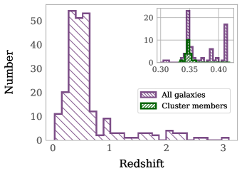
Figure 10: Spectroscopic redshift histogram for galaxies up to $z$ = 3 for the 273 redshifts drawn from all available sources. A peak appears at the cluster redshift of 0.348. A total of 39 galaxies meet the velocity criterion for cluster membership, of which only half meet also the radial cut (green-hashed histogram in the inset plot). We note that a smaller peak is identified at the slightly higher redshift of $z$ = 0.41. On further investigation, the vast majority of these galaxies are situated at large clustercentric radii of ${}^{>}_{\sim}$1 Mpc. These galaxies may be part of a larger scale structure, but are not expected to contribute a significant strong lensing effect.

6.2 The Master Spectroscopic Sample

We combine the MMT/Binospec redshifts with other redshifts available in the literature (F19 and SDSS DR-16), which sum up to 273 spectroscopic redshifts. Cluster membership is met for galaxies which have velocities within $\pm$ 4000 km s^-1 about the mean value of $z$ = 0.348. This corresponds to range of 0.330 $<$ $z$ $<$ 0.366. We choose $\pm$ 4000 km s^-1 so as to include sources in the outskirts of this cluster with its somewhat elongated structure. Of the 273 redshifts, 39 galaxies make the redshift cut. We further downselect to the subset of galaxies whose clustercentric radii are within 1 Mpc. By these criteria, a total of 21 galaxies are admitted to the master cluster member catalog (Figure 10, inset). They are comprised of 8 galaxies from MMT/Binospec (this study), 6 galaxies from Gemini/GMOS (F19), 5 galaxies from MMT/Hectospec (F19), and 2 galaxies from the SDSS DR 16.

The vast majority of cluster members lie reasonably well on the cluster red sequence indicated in Figure 8. The one outlier, a faint elliptical galaxy with $i_{AB}$ = 22.4 mag, is situated in the outskirts of a luminous galaxy at $z$ = 0.033 (SDSS, DR16) that skews its color. Thirteen cluster members are contained in the FOV of this study, which is the field of intersection of the 7-band filter suite roughly comparable to the HST WFC3-IR FOV. This number is a factor of three improvement relative to the number of cluster members reported in the same FOV in F19. Of the 18 cluster members in their study at any clustercentric radius, three are removed from consideration in our new member catalog. They are: “s7” from MMT/Hectospec, whose spectrum had an insecure redshift, “s57” from Gemini/GMOS catalog, and “s35” from the SDSS catalog which were both made redundant by our new MMT/Binospec catalog. There are a set of 22 galaxies which have spectroscopic redshifts behind the cluster of 0.398 $<$ $z$ $<$ 0.426. Of these, only one is situated within a clustercentric radius corresponding to the FOV of this study, and the vast majority (18 of 22) are situated at clustercentric radii greater than 1 Mpc. These galaxies are interesting because they may be part of a larger scale structure, but are not expected to make a significant contribution to the strong lensing model presented here.

The velocities of the cluster members in the common field of interest of 600 kpc are binned and plotted in Figure 11, where for reference 0 km s^-1 marks the cluster’s systemic velocity and the solid vertical line marks the velocity of the brightest cluster galaxy. Although G165 is a visual double-cluster, it is a challenge to separate out the two halves based on their relative velocities. Within radii of 600 kpc and 1 Mpc we measure velocity dispersions of 1040 $\pm$ 282 km s^-1 and 1010 $\pm$ 209 km s^-1, respectively. We calculate the mass by applying the virial theorem via the Gapper method (Wainer & Thissen, 1976; Beers et al., 1990). We obtain masses of (4.9 $\pm$ 2.6) $\times$10¹⁴ M_⊙ within 600 kpc, and (4.6 $\pm$ 1.9) $\times$10¹⁴ M_⊙ within a radius of $\sim$1 Mpc, where the uncertainty is computed by a jackknife sampling following the prescription in Beers et al. (1990). These values are consistent with each other and with the mass estimated from the lens model to within the stated uncertainties. If the hint of an increase in the mass with increasing radius turns out to be real, then we will have a velocity indicator that this system that is not virialized. We refer also to Ferragamo et al. (2020) for a discussion on the biases inherent to estimating masses based on velocity dispersions. We refer to §8 for a discussion of the cluster kinematics, and to Golovich et al. (2017) for a review of the pitfalls entailed with the approach to detect some mergers by the non-Gaussian shapes of their velocities alone.

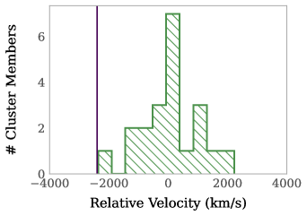
Figure 11: Histogram of the velocities of the confirmed cluster members in the common field that is covered by all of the data of 600 kpc (green-hashed histogram of the inset of Figure 10), plotted relative to the velocity center. The BCG is marked by the green vertical line at -2400 km s^-1. The velocities describe a roughly normal distribution, despite the cluster’s visual bimodality. As such, the large velocity offset of the BCG suggests a cluster disturbance. Additional clues as to the cluster’s dynamical state are discussed in §8.

7 Revised Lens Model

We use the well-tested light traces mass (LTM) approach to construct the 2D projected mass map as is used in F19 (Zitrin et al., 2009, 2015). This semi-parametric method assumes the galaxies are tracers of the dark matter, which for the case of G165 was shown to produce results consistent with non-parametric methods (F19). The inputs are the photometry and positions of the cluster members, and the redshifts of the lens and multiply-imaged sources. The cluster member observables inform the placement of power-law surface density profiles which are scaled based on the galaxy brightnesses. The superposition of these density profiles is smoothed with a Gaussian kernel to approximate the smooth dark matter distribution of the cluster. The cluster member density profiles are assigned a relative weight with respect to the dark matter. In turn, the total mass distribution is approximated as the sum of the smooth dark matter and the galaxy power law surface density profiles scaled by the galaxy relative weights. Additional parameters include values for external shear, shear orientation, individual galaxy weights, individual galaxy ellipticities and position angles, and arc family redshifts.

The free parameters are fit for via a MCMC minimization using thousands of steps to produce the final model. Errors are computed by bootstrapping the MCMC steps, sampling 100 random realizations in the MCMC and quoting the Gaussian errors. We stress that the MCMC errors are not robust to changes in the lensing constraints, and are purely statistical. Strong lens modeling is an intrinsically underconstrained problem, and the statistical errors will ultimately underestimate the true error which is dominated by the systematics (Johnson & Sharon, 2016; Meneghetti et al., 2017; Strait et al., 2018).

7.1 Image System Designations

We retain the same image system designations as in F19, with the exception that Arcs 1a,b are renamed as Arcs 1a/b,c. The Arc 1a/b nomenclature is preferred because it acknowledges that there are two contiguously-positioned images of this one lensed source. To remove ambiguity, it follows that the arc formerly named as Arc 1b is changed to Arc 1c. All image systems identified and used by the model are labeled in Figure 12.

7.2 The G165 Model

We introduce herein new photometric redshift information for Arcs 2a,c and Arcs 11a,b to refine the mass map in F19 that was anchored on a single spectroscopic redshift of a single image of a single system, Arc 1a/b. We also update the cluster member list as described in §5.2. We construct the model by fixing the Arc 1a/b redshift, and updating the constraints on Arcs 2 and 11, leaving their redshifts free to vary only within the $1\sigma$ uncertainty of its associated photometric redshift. The redshifts of all other arc systems (systems 3-10) are left to be optimized by the model without constraints. We fix the weights of all cluster members within the LTM algorithm on the basis of their brightnesses, with the exception of the BCG, whose weight is left free to be optimized by the model. The new photometric and spectroscopic redshifts of the cluster members and arcs introduce additional constraints, which result in an improvement to the lens model.

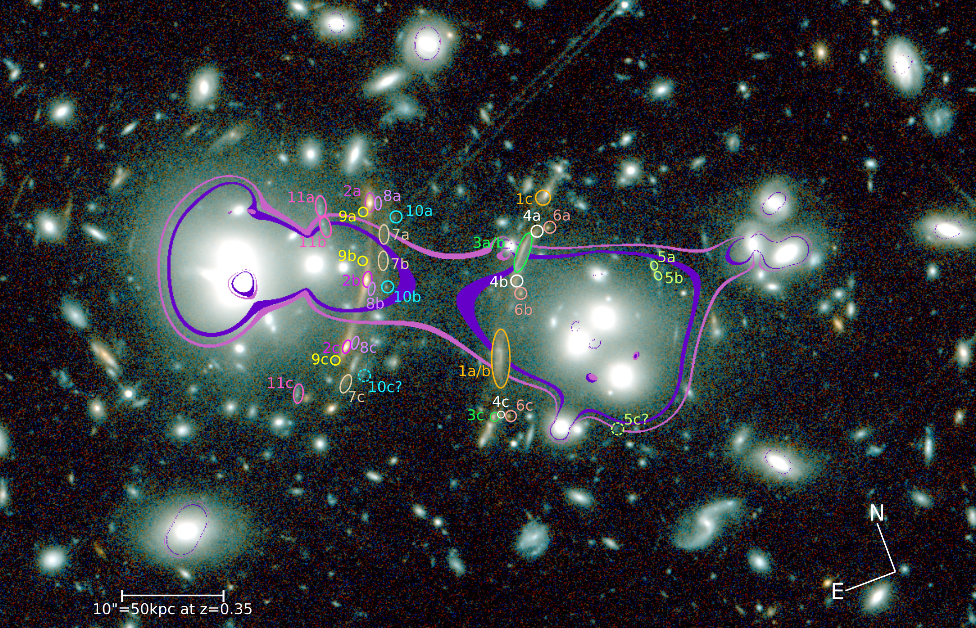
Figure 12: Composite two-color $F110W$ and $F160W$ image showing the $z$ = 2.2 (inner purple; equating to the redshift of Arc 1a/b) and the $z$ = 4.8 (outer pink; equating to the redshift of Arcs 11a,b) critical curves for the LTM lens model that incorporates the new photometric redshift estimates obtained in this study. The critical curves are determined as an absolute magnification cutoff in log space. All images of a single background galaxy are coded to the same color. Several arcs fold about the critical curve (e.g., Arcs 1, 2, 3, 5, 7, 11), making this cluster potentially well-suited to the detection of caustic transients.

The best model, which is the one for which $\chi^{2}$ is minimized, is presented in Figure 12. Critical lines are overlaid for $z$ = 2.2 (equating to the redshift of Arc 1a/b) and $z$ = 4.8 (equating to the redshift of Arcs 11a,b) which delineate the elongated configuration and bimodal mass distribution. The revised model has a smaller measured area within the critical line when compared to the initial model in F19 by $\sim$20 %. We estimate the lensing mass based on the MCMC to be $(2.36\pm 0.23)\times$ $10^{14}M_{\odot}$ within 600 kpc. For this model we predict input image constraints to an RMS recovery angular position of $\sim$ 0.6^′′. The model acquires improved functionality also for testing the positions of the image systems in F19. The image designations of Arc 5c and Arc 10c, which were plausible but unconfirmed in F19, remain as such in this study. At the same time, the updated model reduces the likelihood of the Arc 9 counterimages, 9d and 9e. We do not uncover any new image multiplicities. We discuss the high redshift population in §7.3.

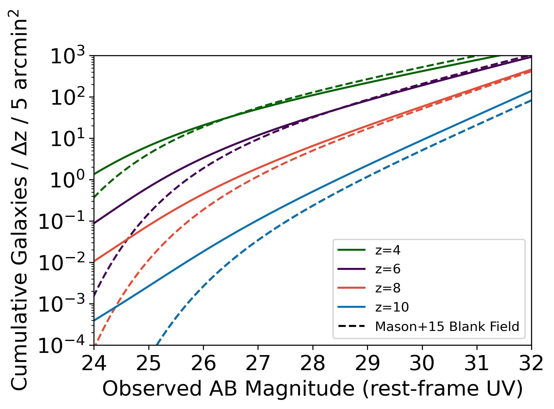
Figure 13: Cumulative number counts of lensed galaxies expected to be detected for different redshifts given a limiting AB magnitude and assuming a complete survey (continuous lines). We make a comparison with the blank field luminosity functions as measured by Mason et al. (2015), which we extrapolate beyond the $17.5<M_{AB}<22.5$ fitting range (dashed lines). In these models, the cumulative distribution is integrated down to the lower limit of the fitting range of 17.5 AB mag. G165 remains a powerful lensing cluster with a high predicted galaxy count at high redshifts in the planned JWST observations of limiting magnitude 29 AB mag.

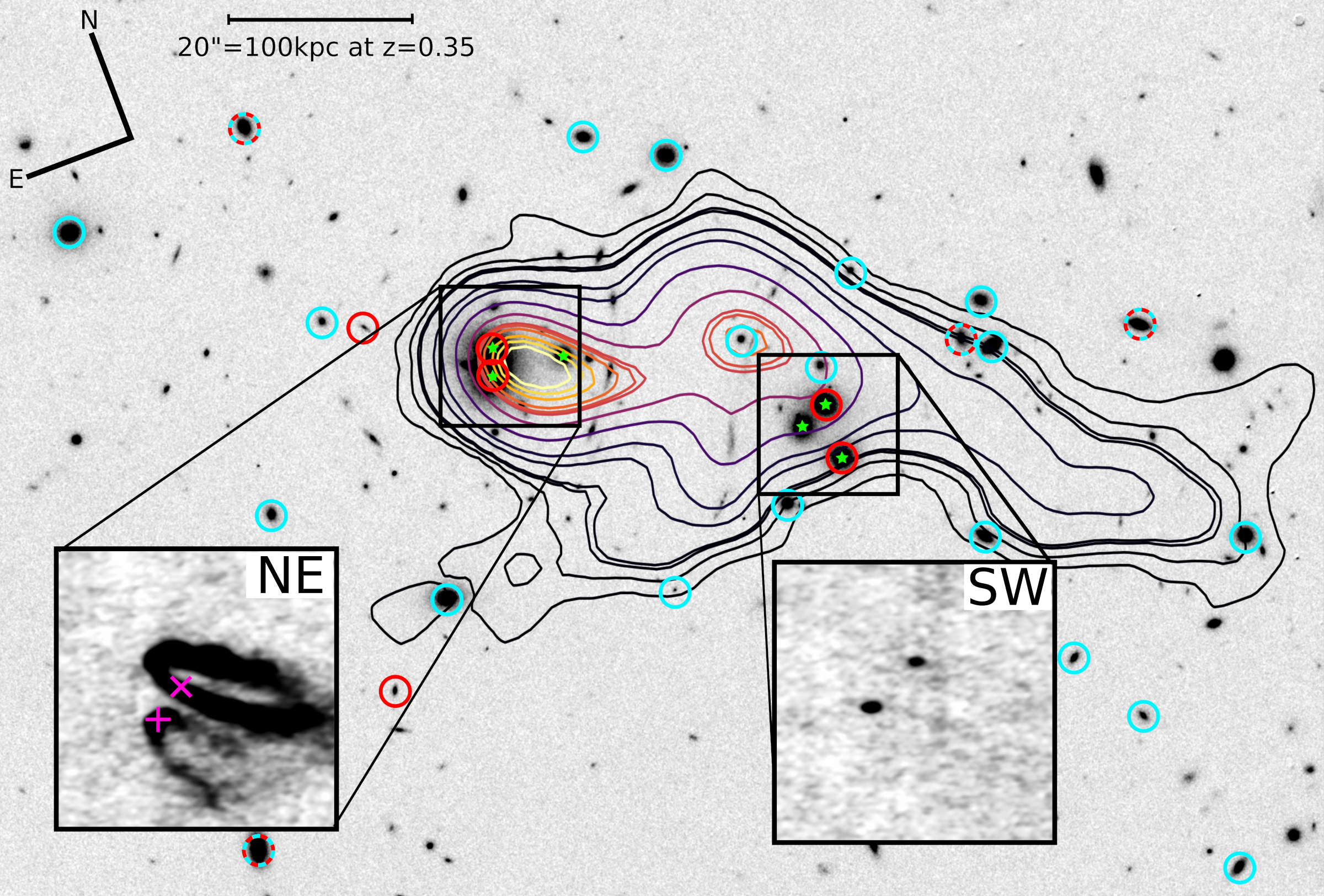
Figure 14: LUCI-Argos $K$ band image depicting spectroscopically confirmed cluster members (0.33 $\leq$ $z_{spec}$ $\leq$ 0.36, red circles), photometrically confirmed cluster members ($0.3\leq z_{phot}\leq 0.4$, blue circles), and the set of six dominant galaxy members (green stars). The insets depict the VLA 6 GHz images in 15^′′ $\times$ 15^′′ patches centered on the SW and NE sides, as indicated. The BCG (magenta ‘+’), and luminosity weighted mean of the cluster (magenta ‘x’), are offset from each other. The velocity of the BCG is also offset from the velocity mean, all of which suggest a dynamical disturbance. The LOFAR radio data (contours) recover the two central peaks, and show tails extending to the southwest and to the east with a physical extent of $\sim$ 500 kpc. Two prominent head-tail galaxies are detected in the NE side of the VLA radio map. These galaxies are identified with the BCG and an LRG, whose jet orientations suggest a post-core passage. Based on the available information, this cluster appears to be undergoing a merger in a direction roughly transverse to the LOS.

7.3 Predicted Galaxy Number Counts

G165 remains a powerful lensing cluster, with a 2D projected mass estimate derived from our strong lensing model of $M_{600kpc}\,=\,(2.36\pm 0.23)\times$ $10^{14}M_{\odot}$, and a $z$ = 9 Einstein radius of $\theta_{E}$ $\approx$ 15.3^′′ that is comparable in strength to HFF cluster Abell 2744. We apply our revised model here in order to make predictions for the galaxy number counts extending to higher redshifts. This serves to place a check on the recovered photometric redshifts, as well as characterize the lensing strength implied by the model. Figure 13 shows the cumulative number counts of lensed galaxies observed within a 5 $\text{arcmin}^{2}$ FOV centered on G165 as a function of magnitude. We opt for the Mason et al. (2015) luminosity function to represent the blank field because it can accommodate a wide range of redshifts, as indicated. One result is that the lensed source counts do not win out over the field galaxy counts at all redshifts and limiting magnitudes. Even so, the number of lensed galaxies gains over the number of field galaxies with increasing mean redshift. This is because the faint end of the luminosity function flattens with increasing redshift, such that the loss of sources by field dilation is compensated for by the detection of sources which rise up above the apparent limiting magnitude.

Given the limiting AB magnitude of 27 of our HST data, the lensed luminosity function predicts order unity detections of $z\approx 6$ and $z\approx 8$ galaxies, and dozens of $z\approx 4$ galaxies. As shown in the results of Table 2, we detect only one $z\approx 6$ galaxy and a handful of $z\approx 4-5$ galaxies. While the predictions are only rough estimates, the lower numbers of observed detections are in part owing to incompleteness of the catalog, as Figure 13 represents an idealized survey. Morever, although the detections made in the mixed bag of 7 bands of imaging with differing image characteristics and qualities presented here are the best available, they are not ideal for churning out large numbers of quality photometric redshifts. Increasing the number of filters to improve spectral coverage at high resolution, and increasing the depth of the 3.6 $\mu$m and 4.5 $\mu$m filters beyond 23 AB mag will help to obtain a more complete photometric redshift catalog. Looking toward the planned observations of G165 using JWST/NIRCam, a limiting magnitude of 29 AB will be achieved in 8 bands, yielding $\sim$100 sources at $z$ $\approx$ 4, and order unity sources at $z$ $\approx$ 10.

7.4 Arcs 1a/b, 1c

The DSFG Arc 1a/b ($z=2.2$) is relatively-faint in the near-IR ($F160W_{ab}$ = 22.23 mag) and red ($g$ $-$ $i$ =  0.9 AB mag), as expected of a dust-obscured source. The high magnification factor derived from our revised lens model of $\mu$ $\approx 25$ stretches this galaxy out to an angular extent of $\sim$ 5^′′, enabling a privileged view at the kpc scale into the interstellar medium of a high-redshift star forming galaxy. Arc 1a/b is detected in the rest-frame ultraviolet, corresponding to observed $g$-band (23.4 $\pm$ 0.1 AB mag). From this we infer that there is at least some leakage of ultraviolet light from massive stars. DSFGs are highly dust-extincted, yet lensing may offer the advantage of stretching out the light into more pixels to achieve better sampling, which may allow the transmission of ultraviolet light. Although unresolved, the sources of this UV starlight appear to be the star forming knots (Figure 12). One counter image is detected, Arc 1c, but it is faint and drops out of detection in the three bluest filters, disallowing the estimation of a photometric redshift. Preliminary images acquired using the VLA detect Arc 1c, and separate out what appear to be the star forming regions of Arc 1a/b into four knots, two each on opposite sides of the critical curve. These results will appear in an upcoming paper (Kamieneski et al. 2022, in preparation).

8 Cluster Evolutionary State

8.1 The O/IR Picture

Our data gives clues as to the state of virialization of this cluster. We are given: (1) the photometric catalog of 22 member galaxies which cover the range 0.3 $<$ $z_{\text{phot}}$ $<$ 0.4 out to $\sim$ 600 kpc, (2) the spectroscopic catalog of 21 cluster galaxies which covers the range 0.330 $<$ $z$ $<$ 0.366 within 1 Mpc, (3) the combined catalog of the four galaxies with both spectroscopic and photometric redshifts, and (4) the set of six central dominant galaxies. These six galaxies consist of three cluster members in the northeast (NE) component, and three cluster members in the southwest (SW) component (green stars in Figure 14). Although it is useful to further subdivide the cluster membership by galaxy activity levels and galaxy colors, such designations are limited given the small numbers of objects. Below we measure the quantities available to us which were demonstrated by Rumbaugh et al. (2018) to be correlated with cluster virialization: the offset of the luminosity mean center from the BCG and from the velocity center.

We identify the BCG as the cluster member with the highest luminosity as measured in $i$-band (“+” symbol in Figure 14. The $i$-band is selected because it is redder than the 4000 Å and Balmer breaks at the cluster redshift. The mean projected centroid of the cluster member luminosities is computed, from which we obtain the luminosity weighted mean center (LWMC; “x” symbol in Figure 14). The two centers are offset by 3.3 arcseconds, equating to 16.5 kpc. We note that although the $i$-band alone does not fairly represent the stellar mass, the FOV of the near-IR filters is too narrow to cover the full cluster member catalog (Figure 1). We do not undertake an analysis of the individual galaxy masses, nor compute a cluster mass centroid, because the set of 22 galaxies with fitted SEDs does not include certain crucial members such as the BCG and some of the LRGs.

The velocity histogram of the cluster members has a single broad peak. This suggests that the two sides are moving transverse to the line-of-sight. Three of the four central dominant members with spectroscopic redshifts have minimal pair-wise velocity offsets of ${}^{<}_{\sim}$ 100 km s^-1 (red circles in Figure 14), providing further support that the major axis of the cluster is aligned preferentially in the plane of the sky. Intriguingly, the BCG is blueshifted by 2400 km s^-1 relative to the velocity center (Figure 11). The BCG has all the spectroscopic features expected of a passively-evolving elliptical galaxy, from the prominent 4000 Å and Balmer breaks, to the G-band and Balmer lines in absorption. What is unexpected is the large velocity difference between the BCG and the cluster’s systemic velocity. It is interesting that, despite its designation as the BCG, there are no spectroscopically-confirmed neighbors at a similar velocity (to within 1000 km s^-1). Additional longslit spectroscopy centered on the BCG would be advantageous to search for its entourage.

8.2 The Radio Picture

Our radio maps corroborate the general picture of a cluster disturbance, and give clues as to the direction of motion of the NE and SW components. The LOFAR LoTSS map depicts emission with a physical extent of $\sim$500 kpc that is elongated along the major-axis of the cluster. There are two dominant radio peaks, one roughly centered on each of the NE and the SW components. An elongated region of somewhat more diffuse radio emission extends to the southwest of the SW peak with a physical extent 300 kpc, and a shelf-like emission feature is detected protruding to the east. A distinctive comet-like morphology of the NE peak trails off into the southwesterly direction.

At the higher resolution of the VLA 6 GHz radio map, the NE peak separates out into two head-tail galaxies: one corresponding to the BCG and the other to an LRG (NE inset in Figure 14). The VLA map also detects two LRGs in the SW side as more compact radio sources in the same pointing, and all within the primary beam. The trails of each of the two head-tail galaxies are associated with an active galactic nucleus in the center of each galaxy that is ejecting a bipolar jet.

These Narrow Angle Tails (NATs)

(e. g., Müller et al., 2021) are relatively common in galaxy cluster fields (e. g., Malavasi et al., 2016; Garon et al., 2019). Interestingly, in the G165 field the trails of the two NATs are also more-or-less aligned with each other, a behavior that suggests a common ensemble jet motion. Given that a NAT will typically occupy the wake of its host,

we infer that the radio jets are being swept back from the northeast direction by ram pressure.

Curiously, G165 is not X-ray bright despite participating in an ongoing merger that should have shock-heated the intercluster gas to X-ray temperatures. In order to maintain the lower X-ray luminosity it is tempting to speculate that the two components may not have directly impacted each other, but instead achieved a longer distance cluster-cluster interaction.

The near-alignment of both pairs of radio trails suggests an ensemble motion that is not along the line-of-sight, making the transverse velocity nonzero (Gendron-Marsolais et al., 2020). There is not yet enough information to measure its value, but there are some clues. In a study incorporating the results of NATs in both poor and rich galaxy clusters, Venkatesan et al. (1994) find the appearance of NATs in all cases, and estimate typical NAT velocities of $\sim$ 600 km s^-1 to be able to form its distinctive morphology. In the large N-body dark-matter only numerical simulation, the JUropa Hubble volumE (Jubilee; Watson et al., 2014), they consider examples of merging halo pairs in the $z$ = 0.32 redshift slice that is well-matched to that of G165. Although the velocity scatter is large, and the halo separations are less well sampled at ${}^{<}_{\sim}$ 0.6 Mpc, an extrapolation to smaller halo separations indicates that typical pair-wise velocities of halo-halo mergers are ${}^{>}_{\sim}$100 km s^-1 (Watson et al., 2014). In another recent study of three HFFs, space velocities at regular intervals in the range of 500 – 5000 km s^-1 are inserted to the measured velocities of the cluster members and its deviation from the line-of-sight velocity distribution recorded. By this kinematical analysis, an upper limit on the transverse velocity of 1700 km s^-1 is allowed in order to still recover the observed line-of-sight velocity distribution (Windhorst et al., 2018). These studies suggest that the transverse velocity of G165 may be in the 100–1700 km s^-1 range. X-ray observations will enable a study of the collision properties, and improved constraints regarding the viewing angle and transverse velocity.

9 Conclusions

G165 is a powerful lensing cluster with a bimodal mass distribution, rich lensing evidence, and low X-ray luminosity. Upon incorporating the new LBT/LBC and Spitzer imaging data, photometric redshifts are enabled for three image multiplicities. New MMT/Binospec spectroscopy contributed eight additional cluster members. These lensing constraints produced a lens model that refined the placement of the critical curve relative to the caustic-crossing arcs and but falls short of detecting the subhalo underlying the BCG velocity outlier.

The detection of the four radio trails in a roughly mutual alignment suggests an impact orientation in the plane of the sky and a direction of motion in the northeast-southwest direction. In this scenario, the NE and SW components have already traversed each other in an event that instigated the radio activity and supplied the pressure for the cluster gas to sweep past the radio jets. Here the low X-ray luminosity is explained by a more indirect cluster-cluster encounter of the NE and SW components.

High-resolution blue imaging is needed to constrain the age of the merger by its rest-frame ultraviolet-optical colors, and X-ray observations enable searches for shocks to establish the collision speed. The only way to uncover all halos participating in the cluster merger is by obtaining additional lensing evidence by deep high-resolution imaging in the planned JWST/NIRCam PEARLS-Clusters approved program.

Ultimately, such observations offer a viable route to constrain the evolutionary state of this binary cluster that in turn contributes to our understanding of mass assembly on cluster scales.

References

- Ahumada et al. (2020) Ahumada, R., Prieto, C. A., Almeida, A., et al. 2020, ApJS, 249, 3, doi: 10.3847/1538-4365/ab929e
- Astropy Collaboration et al. (2013) Astropy Collaboration, Robitaille, T. P., Tollerud, E. J., et al. 2013, A&A, 558, A33, doi: 10.1051/0004-6361/201322068
- Astropy Collaboration et al. (2018) Astropy Collaboration, Price-Whelan, A. M., Sipőcz, B. M., et al. 2018, AJ, 156, 123, doi: 10.3847/1538-3881/aabc4f
- Barden et al. (2012) Barden, M., Häußler, B., Peng, C. Y., McIntosh, D. H., & Guo, Y. 2012, MNRAS, 422, 449, doi: 10.1111/j.1365-2966.2012.20619.x
- Beers et al. (1990) Beers, T. C., Flynn, K., & Gebhardt, K. 1990, AJ, 100, 32, doi: 10.1086/115487
- Benítez (1999) Benítez, N. 1999, in Astronomical Society of the Pacific Conference Series, Vol. 191, Photometric Redshifts and the Detection of High Redshift Galaxies, ed. R. Weymann, L. Storrie-Lombardi, M. Sawicki, & R. Brunner, 31
- Benítez (2000) Benítez, N. 2000, ApJ, 536, 571, doi: 10.1086/308947
- Benítez et al. (2004) Benítez, N., Ford, H., Bouwens, R., et al. 2004, ApJS, 150, 1, doi: 10.1086/380120
- Beroiz et al. (2020) Beroiz, M., Cabral, J. B., & Sanchez, B. 2020, Astronomy and Computing, 32, 100384, doi: 10.1016/j.ascom.2020.100384
- Bertin (2006) Bertin, E. 2006, in Astronomical Society of the Pacific Conference Series, Vol. 351, Astronomical Data Analysis Software and Systems XV, ed. C. Gabriel, C. Arviset, D. Ponz, & S. Enrique, 112
- Bertin (2010) Bertin, E. 2010, SWarp: Resampling and Co-adding FITS Images Together. http://ascl.net/1010.068
- Bertin & Arnouts (1996) Bertin, E., & Arnouts, S. 1996, A&AS, 117, 393, doi: 10.1051/aas:1996164
- Bertin et al. (2002) Bertin, E., Mellier, Y., Radovich, M., et al. 2002, in Astronomical Society of the Pacific Conference Series, Vol. 281, Astronomical Data Analysis Software and Systems XI, ed. D. A. Bohlender, D. Durand, & T. H. Handley, 228
- Bradac et al. (2019) Bradac, M., Huang, K.-H., Fontana, A., et al. 2019, MNRAS, 489, 99, doi: 10.1093/mnras/stz2119
- Bradley et al. (2020) Bradley, L., Sipőcz, B., Robitaille, T., et al. 2020, astropy/photutils: 1.0.0, 1.0.0, Zenodo, doi: 10.5281/zenodo.4044744
- Broadhurst et al. (2005) Broadhurst, T., Benítez, N., Coe, D., et al. 2005, ApJ, 621, 53, doi: 10.1086/426494
- Bruzual & Charlot (2003) Bruzual, G., & Charlot, S. 2003, MNRAS, 344, 1000, doi: 10.1046/j.1365-8711.2003.06897.x
- Cañameras et al. (2015) Cañameras, R., Nesvadba, N. P. H., Guery, D., et al. 2015, A&A, 581, A105, doi: 10.1051/0004-6361/201425128
- Cañameras et al. (2018) Cañameras, R., Nesvadba, N. P. H., Limousin, M., et al. 2018, A&A, 620, A60, doi: 10.1051/0004-6361/201833679
- Casertano et al. (2000) Casertano, S., de Mello, D., Dickinson, M., et al. 2000, AJ, 120, 2747, doi: 10.1086/316851
- Castellano et al. (2016) Castellano, M., Amorín, R., Merlin, E., et al. 2016, A&A, 590, A31, doi: 10.1051/0004-6361/201527514
- Chen et al. (2019) Chen, W., Kelly, P. L., Diego, J. M., et al. 2019, ApJ, 881, 8, doi: 10.3847/1538-4357/ab297d
- Coe et al. (2006) Coe, D., Benítez, N., Sánchez, S. F., et al. 2006, AJ, 132, 926, doi: 10.1086/505530
- Coe et al. (2013) Coe, D., Zitrin, A., Carrasco, M., et al. 2013, ApJ, 762, 32, doi: 10.1088/0004-637X/762/1/32
- Coleman et al. (1980) Coleman, G. D., Wu, C. C., & Weedman, D. W. 1980, ApJS, 43, 393, doi: 10.1086/190674
- Dahlen et al. (2013) Dahlen, T., Mobasher, B., Faber, S. M., et al. 2013, ApJ, 775, 93, doi: 10.1088/0004-637X/775/2/93
- Dai & Miralda-Escudé (2020) Dai, L., & Miralda-Escudé, J. 2020, AJ, 159, 49, doi: 10.3847/1538-3881/ab5e83
- Dai et al. (2018) Dai, L., Venumadhav, T., Kaurov, A. A., & Miralda-Escud, J. 2018, ApJ, 867, 24, doi: 10.3847/1538-4357/aae478
- Dai et al. (2020) Dai, L., Kaurov, A. A., Sharon, K., et al. 2020, MNRAS, 495, 3192, doi: 10.1093/mnras/staa1355
- De Santis et al. (2007) De Santis, C., Grazian, A., Fontana, A., & Santini, P. 2007, New A, 12, 271, doi: 10.1016/j.newast.2006.10.004
- Diego et al. (2018) Diego, J. M., Kaiser, N., Broadhurst, T., et al. 2018, ApJ, 857, 25, doi: 10.3847/1538-4357/aab617
- Erben et al. (2005) Erben, T., Schirmer, M., Dietrich, J. P., et al. 2005, Astronomische Nachrichten, 326, 432, doi: 10.1002/asna.200510396
- Ferragamo et al. (2020) Ferragamo, A., Rubiño-Martín, J. A., Betancort-Rijo, J., et al. 2020, A&A, 641, A41, doi: 10.1051/0004-6361/201834837
- Franx et al. (1997) Franx, M., Illingworth, G. D., Kelson, D. D., van Dokkum, P. G., & Tran, K.-V. 1997, ApJ, 486, L75, doi: 10.1086/310844
- Frye & Broadhurst (1998) Frye, B., & Broadhurst, T. 1998, ApJ, 499, L115, doi: 10.1086/311361
- Frye et al. (2019) Frye, B., Pascale, M., Qin, Y., et al. 2019, The Astrophysical Journal, 871, 51, doi: 10.3847/1538-4357/aaeff7
- Frye et al. (2012) Frye, B. L., Hurley, M., Bowen, D. V., et al. 2012, ApJ, 754, 17, doi: 10.1088/0004-637X/754/1/17
- Fujimoto et al. (2021) Fujimoto, S., Oguri, M., Brammer, G., et al. 2021, ApJ, 911, 99, doi: 10.3847/1538-4357/abd7ec
- Gaia Collaboration et al. (2016) Gaia Collaboration, Prusti, T., de Bruijne, J. H. J., et al. 2016, A&A, 595, A1, doi: 10.1051/0004-6361/201629272
- Galametz et al. (2013) Galametz, A., Grazian, A., Fontana, A., et al. 2013, ApJS, 206, 10, doi: 10.1088/0067-0049/206/2/10
- Garon et al. (2019) Garon, A. F., Rudnick, L., Wong, O. I., et al. 2019, AJ, 157, 126, doi: 10.3847/1538-3881/aaff62
- Gendron-Marsolais et al. (2020) Gendron-Marsolais, M., Hlavacek-Larrondo, J., van Weeren, R. J., et al. 2020, MNRAS, 499, 5791, doi: 10.1093/mnras/staa2003
- Ghosh et al. (2020) Ghosh, A., Williams, L. L. R., & Liesenborgs, J. 2020, MNRAS, 494, 3998, doi: 10.1093/mnras/staa962
- Giallongo et al. (2014) Giallongo, E., Menci, N., Grazian, A., et al. 2014, ApJ, 781, 24, doi: 10.1088/0004-637X/781/1/24
- Golovich et al. (2017) Golovich, N., Dawson, W. A., Wittman, D. M., et al. 2017, arXiv e-prints, arXiv:1711.01347. https://arxiv.org/abs/1711.01347
- Griffiths et al. (2018) Griffiths, A., Conselice, C. J., Alpaslan, M., et al. 2018, MNRAS, 475, 2853, doi: 10.1093/mnras/stx3364
- Harrington et al. (2016) Harrington, K. C., Yun, M. S., Cybulski, R., et al. 2016, MNRAS, 458, 4383, doi: 10.1093/mnras/stw614
- Harrington et al. (2021) Harrington, K. C., Weiss, A., Yun, M. S., et al. 2021, ApJ, 908, 95, doi: 10.3847/1538-4357/abcc01
- Johnson & Sharon (2016) Johnson, T. L., & Sharon, K. 2016, ApJ, 832, 82, doi: 10.3847/0004-637X/832/1/82
- Jullo et al. (2007) Jullo, E., Kneib, J. P., Limousin, M., et al. 2007, New Journal of Physics, 9, 447, doi: 10.1088/1367-2630/9/12/447
- Kaurov et al. (2019) Kaurov, A. A., Dai, L., Venumadhav, T., Miralda-Escudé, J., & Frye, B. 2019, ApJ, 880, 58, doi: 10.3847/1538-4357/ab2888
- Kelly et al. (2018) Kelly, P. L., Diego, J. M., Rodney, S., et al. 2018, Nature Astronomy, 2, 334, doi: 10.1038/s41550-018-0430-3
- Kinney et al. (1996) Kinney, A. L., Calzetti, D., Bohlin, R. C., et al. 1996, ApJ, 467, 38, doi: 10.1086/177583
- Kneib et al. (2004) Kneib, J.-P., Ellis, R. S., Santos, M. R., & Richard, J. 2004, ApJ, 607, 697, doi: 10.1086/386281
- Kneib & Natarajan (2011) Kneib, J.-P., & Natarajan, P. 2011, A&A Rev., 19, 47, doi: 10.1007/s00159-011-0047-3
- Malavasi et al. (2016) Malavasi, N., Bardelli, S., Ciliegi, P., et al. 2016, in Astrophysics and Space Science Proceedings, Vol. 42, The Universe of Digital Sky Surveys, ed. N. R. Napolitano, G. Longo, M. Marconi, M. Paolillo, & E. Iodice, 109, doi: 10.1007/978-3-319-19330-4_17
- Mason et al. (2015) Mason, C. A., Trenti, M., & Treu, T. 2015, ApJ, 813, 21, doi: 10.1088/0004-637X/813/1/21
- McMullin et al. (2007) McMullin, J. P., Waters, B., Schiebel, D., Young, W., & Golap, K. 2007, in Astronomical Society of the Pacific Conference Series, Vol. 376, Astronomical Data Analysis Software and Systems XVI, ed. R. A. Shaw, F. Hill, & D. J. Bell, 127
- Meneghetti et al. (2017) Meneghetti, M., Natarajan, P., Coe, D., et al. 2017, MNRAS, 472, 3177, doi: 10.1093/mnras/stx2064
- Merlin et al. (2015) Merlin, E., Fontana, A., Ferguson, H. C., et al. 2015, A&A, 582, A15, doi: 10.1051/0004-6361/201526471
- Merlin et al. (2016) Merlin, E., Amorín, R., Castellano, M., et al. 2016, A&A, 590, A30, doi: 10.1051/0004-6361/201527513
- Merlin et al. (2021) Merlin, E., Castellano, M., Santini, P., et al. 2021, A&A, 649, A22, doi: 10.1051/0004-6361/202140310
- Miralda-Escude (1991) Miralda-Escude, J. 1991, ApJ, 379, 94, doi: 10.1086/170486
- Müller et al. (2021) Müller, A., Pfrommer, C., Ignesti, A., et al. 2021, MNRAS, 508, 5326, doi: 10.1093/mnras/stab2928
- Nagy et al. (2021) Nagy, D., Dessauges-Zavadsky, M., Richard, J., et al. 2021, arXiv e-prints, arXiv:2109.06206. https://arxiv.org/abs/2109.06206
- Nesvadba et al. (2019) Nesvadba, N. P. H., Cañameras, R., Kneissl, R., et al. 2019, A&A, 624, A23, doi: 10.1051/0004-6361/201833777
- Oguri et al. (2018) Oguri, M., Diego, J. M., Kaiser, N., Kelly, P. L., & Broadhurst, T. 2018, Phys. Rev. D, 97, 023518, doi: 10.1103/PhysRevD.97.023518
- Pagul et al. (2021) Pagul, A., Sánchez, F. J., Davidzon, I., & Mobasher, B. 2021, arXiv e-prints, arXiv:2103.01952. https://arxiv.org/abs/2103.01952
- Peng et al. (2010) Peng, C. Y., Ho, L. C., Impey, C. D., & Rix, H.-W. 2010, AJ, 139, 2097, doi: 10.1088/0004-6256/139/6/2097
- Pilbratt et al. (2010) Pilbratt, G. L., Riedinger, J. R., Passvogel, T., et al. 2010, A&A, 518, L1, doi: 10.1051/0004-6361/201014759
- Planck Collaboration et al. (2015) Planck Collaboration, Aghanim, N., Altieri, B., et al. 2015, A&A, 582, A30, doi: 10.1051/0004-6361/201424790
- Planck Collaboration et al. (2020) Planck Collaboration, Aghanim, N., Akrami, Y., et al. 2020, A&A, 641, A6, doi: 10.1051/0004-6361/201833910
- Rabien et al. (2019) Rabien, S., Angel, J., Barl, L., et al. 2019, Astronomy and Astrophysics, 621, doi: 10.1051/0004-6361/201833716
- Rumbaugh et al. (2018) Rumbaugh, N., Lemaux, B. C., Tomczak, A. R., et al. 2018, MNRAS, 478, 1403, doi: 10.1093/mnras/sty1181
- Schirmer (2013) Schirmer, M. 2013, ApJS, 209, 21, doi: 10.1088/0067-0049/209/2/21
- Sharma et al. (2018) Sharma, S., Richard, J., Yuan, T., et al. 2018, MNRAS, 481, 1427, doi: 10.1093/mnras/sty2352
- Shimwell et al. (2017) Shimwell, T. W., Röttgering, H. J. A., Best, P. N., et al. 2017, A&A, 598, A104, doi: 10.1051/0004-6361/201629313
- Shimwell et al. (2019) Shimwell, T. W., Tasse, C., Hardcastle, M. J., et al. 2019, A&A, 622, A1, doi: 10.1051/0004-6361/201833559
- Soucail et al. (1987) Soucail, G., Mellier, Y., Fort, B., Hammer, F., & Mathez, G. 1987, A&A, 184, L7
- Stetson (1987) Stetson, P. B. 1987, PASP, 99, 191, doi: 10.1086/131977
- Strait et al. (2018) Strait, V., Bradač, M., Hoag, A., et al. 2018, ApJ, 868, 129, doi: 10.3847/1538-4357/aae834
- van Diepen et al. (2018) van Diepen, G., Dijkema, T. J., & Offringa, A. 2018, DPPP: Default Pre-Processing Pipeline. http://ascl.net/1804.003
- Vanzella et al. (2020) Vanzella, E., Meneghetti, M., Pastorello, A., et al. 2020, MNRAS, 499, L67, doi: 10.1093/mnrasl/slaa163
- Venkatesan et al. (1994) Venkatesan, T. C. A., Batuski, D. J., Hanisch, R. J., & Burns, J. O. 1994, ApJ, 436, 67, doi: 10.1086/174881
- Venumadhav et al. (2017) Venumadhav, T., Dai, L., & Miralda-Escudé, J. 2017, ApJ, 850, 49, doi: 10.3847/1538-4357/aa9575
- Wainer & Thissen (1976) Wainer, H., & Thissen, D. 1976, Psychometrika, 41, 9–34, doi: 10.1007/bf02291695
- Watson et al. (2014) Watson, W. A., Diego, J. M., Gottlöber, S., et al. 2014, MNRAS, 438, 412, doi: 10.1093/mnras/stt2208
- Welch et al. (2022) Welch, B., Coe, D., Diego, J., et al. 2022, Nature, in press
- Windhorst et al. (2018) Windhorst, R. A., Timmes, F. X., Wyithe, J. S. B., et al. 2018, ApJS, 234, 41, doi: 10.3847/1538-4365/aaa760
- Zitrin et al. (2009) Zitrin, A., Broadhurst, T., Umetsu, K., et al. 2009, MNRAS, 396, 1985, doi: 10.1111/j.1365-2966.2009.14899.x
- Zitrin et al. (2015) Zitrin, A., Labbé, I., Belli, S., et al. 2015, ApJ, 810, L12, doi: 10.1088/2041-8205/810/1/L12