A possible trial beyond the conventional random phase approximation for the $su(2)$-Lipkin model including the case of non-closed shell system

Abstract

Concerning the $su(2)$-Lipkin model, the calculation of the excitation energy to the 1st excited-state gives rise to the following fact: The two results based on the exact treatment and the conventional random phase approximation (RPA) are in unexpected disagreement. In order to remove this discrepancy, the conventional RPA is renewed. With the aim of this renewal, the terms, which cannot be dealt with in the conventional one, are estimated. The basic framework of this new form is not reorganized from that of the conventional one. In addition, the $su(2)$-Lipkin model itself is also modified so as to be applicable to the case with non-closed shell system. To this modification, one more $su(2)$-algebra, which has been already proposed by the present authors, is applied. Through the use of this algebra, the $su(2)$-Lipkin model is applicable to the case with any total fermion number permitted in the model.

xxxx, xxx

1 Introduction

It is hardly necessary to mention, but the random phase approximation (RPA) has played a central role in various fields of many-body theories. We quote only two papers for the pioneering works 1 . Immediately after the idea of RPA was introduced, theoretical nuclear study changed its nature 2 . This method is based on a certain linearization of the equations of motion for the particle-hole pair creation and annihilation operators. They play a role of the supports in the RPA method. In order to define the particle and the hole operators, the free vacuum is indispensable. It must be of the closed-shell for a given total fermion number, for example, such as the Hartree-Fock (HF) vacuum. Further, for the Hamiltonian widely used, the above-mentioned equations of motion contain the terms related to the bilinear forms of the particles and the holes except the supports in RPA. In the conventional RPA, these terms are replaced with the expectation values for the free vacuum. Through this procedure, we can complete the linearization and we obtain a non-hermitian eigenvalue equation for $\omega$. Here, $\omega$ denotes the frequency of the oscillation, which can be regarded as the excitation energy from the ground-state. If $\omega^{2}>0$, this oscillation is stable around the chosen free vacuum and if $\omega^{2}<0$, unstable. The point $\omega^{2}=0$ is critical from the stable to the unstable, i.e., usually, it is called the phase transition. However, the free vacuum commonly used, in many cases, are in non-closed shell. In the case where the pairing correlation is strong, we can adopt the BCS-Bogoliubov method. In this case, we can formulate the RPA method in the quasi-particle space 3 . The bilinear terms for the quasi-particles except the quasi-particle pairs as the supports in RPA are replaced with the expectation values for the BCS ground-state. The above may be one of the standard understanding of the conventional RPA.

In relation to the above argument, we must pay attention to the $su(2)$-Lipkin model 4 . It supplies a simple model for obtaining the exact results easily such as the excitation energy etc. and, further, for checking the validity of the RPA method. Since this model obeys the $su(2)$-algebra, it is realized by certain bilinear forms in the single-particle fermion operators. It consists of two single-particle levels, each of degeneracy $2\Omega$, separated by energy $2\epsilon$. Let us take up the following case: In the absence of interaction, $2\Omega$ fermion fully occupy the lower level. Then, if we regard this state as the free vacuum, the particle and the hole operators can be defined. If the interaction is switched on, the fermions can jump from the lower level to the upper one and, finally, the $2\Omega$ fermions become to occupy fully the upper level. Naturally, the lower becomes vacant. The above statement tells us that the free vacuum is nothing but the minimum weight state in the $su(2)$-Lipkin model specified by the magnitude of the $su(2)$-spin $s$. If the total fermion number is denoted by $N$, the present free vacuum is governed by the condition $N=2\Omega=2s$. In this paper, we are interested in the case where the condition $N=2\Omega=2s$ is broken.

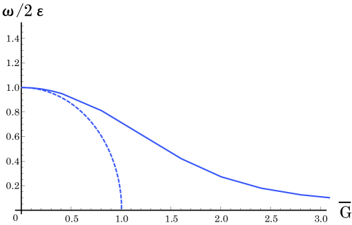
Figure 1: The first excited energies from the ground-state energy are depicted as functions of $\overline{G}=G/\epsilon\cdot 2\Omega$ for exact (solid curve) and the RPA (dashed curve) results with $\Omega=5$.

This paper aims mainly at discussing two subjects. First is to clarify the relationship among the three quantities $N$, $2\Omega$ and $2s$ appearing in the $su(2)$-Lipkin model. For this purpose, we prepare an auxiliary $su(2)$-algebra, three generators of which commute with the three of the original. This $su(2)$-algebra has been already taken up for various purposes by the present authors 5 . With the aid of this algebra, we can modify the $su(2)$-Lipkin model for treating the case where the condition $N=2\Omega=2s$ is broken, i.e., the non-closed shell case. It should be noted that one of the generators is related to the total fermion number operator which the Lipkin model does not contain. Combining these two $su(2)$-algebra, we obtain, for example, the relation $2s\leq N\leq 4\Omega-2s$. Therefore, in the case with $s=\Omega$, automatically, we have $N=2\Omega$. It suggests us that we can treat the cases with $N<2\Omega$ and $N>2\Omega$. The above is the first subject. Second is to develop a possible trial beyond the conventional RPA for the Lipkin model. Figure 1 depicts the frequency $\omega/(2\epsilon)$ given by the conventional RPA and the exactly calculated excitation energy from the ground- to the 1st excited-state as functions of $\overline{G}(=G/\epsilon\cdot 2\Omega)$ for $\Omega=5$. Here, $G$ denotes the strength of the interaction defined in the relation (79). We are forced to see that the discrepancy is quite conspicuous and cannot see any phase transition 6 . For the above situation, we must develop a new idea. In this paper, we will present a possible form for making up the above discrepancy without breaking down the basic framework of the conventional RPA. For this aim, we focus on the parts replaced with the expectation values given by the free vacuum. Our idea is to replace these parts with certain forms obtained through the relation of the Casimir invariant. With the help of this procedure, we can take up the effects let out in the conventional RPA. As an additional remark, we note that the problem discussed in this paper may be old-fashioned, but, until the present, any clear-cut solutions for them have been not obtained. This is our motivation for the present work. Concerning this point, we are interested in the paper7 .

Of course, there are many attempts to extend the RPA itself to include the higher effects such as an anharmonicity from before. For example, in order to extend the HF and RPA methods, the variational approach to the many-body problem was devised by introducing an appropriate trial state and the second RPA was derived in a useful form for obtaining approximate solutionsJdP1 . Also, by using the Green function formalism, the correction to the RPA was derived as a microscopic theory dealing with an anharmonic effectsJdP2 . In the words of the Beliaev-Zelevinsky boson expansion, the generalized RPA was considered by taking into account the boson-boson correlationsJdP3 . Further, it was shown that, if the variational parameters $a$, appearing in the generator-coordinate method, $\Psi(x)=\int\phi(x;a)f(a)da$, depends on the time, the variational parameters oscillate with the same frequency as that derived by the RPAJdP4 , while the relation between the generator-coordinate method and the RPA was indicated in several authorsAdd .

In the next section, a modified form of the $su(2)$-Lipkin model is presented. Another generators of the $su(2)$-algebra adding to the original ones in the $su(2)$-Lipkin model are introduced. In section 3, a renewed random phase approximation is formulated and the non-closed shell system can be treated. The conventional RPA is included in the renewal of the RPA developed in this section. In section 4, various numerical results obtained by the renewed RPA are shown. Especially, the renewed random phase approximation presents a good result for the first-excited energy compared to the conventional RPA. The last section is devoted to concluding remarks.

2 A modified form of the $su(2)$-Lipkin model

The $su(2)$-Lipkin model, which may be the simplest many-fermion model, consists of two single-particle levels with the degeneracies $2\Omega$. Here, $2\Omega$ denotes an integer and we specify the two levels by the index $l$ with $l=0$ and 1. The single-particle states are specified by an appropriate labeling. In this paper, we adopt the labeling $\mu=1,\ 2,\cdots,\ 2\Omega$ for $(0,\mu)$ and $(1,\mu)$. The basic operators in this model are as follows:

$${\widetilde{S}}_{0}=\frac{1}{2}\sum_{\mu}\left({\tilde{c}}_{1\mu}^{*}{\tilde{c}}_{1\mu}-{\tilde{c}}_{0\mu}^{*}{\tilde{c}}_{0\mu}\right)\ ,\quad{\widetilde{S}}_{+}=\sum_{\mu}{\tilde{c}}_{1\mu}^{*}{\tilde{c}}_{0\mu}\ ,\quad{\widetilde{S}}_{-}=\sum_{\mu}{\tilde{c}}_{0\mu}^{*}{\tilde{c}}_{1\mu}\ .$$ (1)

Here, ${\tilde{c}}_{l\mu}^{*}$ and ${\tilde{c}}_{l\mu}$ denote the creation and the annihilation fermion operators in the state $(l,\mu)$, respectively. Needless to say, the hermitian conjugate are given as

$${\widetilde{S}}_{0}^{*}={\widetilde{S}}_{0}\ ,\qquad{\widetilde{S}}_{\pm}^{*}={\widetilde{S}}_{\mp}\ .$$ (2)

The set $({\widetilde{S}}_{0,\pm})$ obeys the $su(2)$-algebra:

$$\left[\ {\widetilde{S}}_{+}\ ,\ {\widetilde{S}}_{-}\ \right]=2{\widetilde{S}}_{0}\ ,\qquad\left[\ {\widetilde{S}}_{0}\ ,\ {\widetilde{S}}_{\pm}\ \right]=\pm{\widetilde{S}}_{\pm}\ .$$ (3)

The Casimir operator ${\widetilde{\boldsymbol{S}}}^{2}$ is given in the form

$${\widetilde{\boldsymbol{S}}}^{2}=\frac{1}{2}\left[\ {\widetilde{S}}_{+}\ ,\ {\widetilde{S}}_{-}\ \right]_{+}+{\widetilde{S}}_{0}^{2}\ .$$ (4)

Naturally, $({\widetilde{S}}_{0,\pm})$ commutes with ${\widetilde{\boldsymbol{S}}}^{2}$.

The Hamiltonian treated in this paper is of the form which has been adopted conventionally:

$${\widetilde{H}}=2\epsilon{\widetilde{S}}_{0}-G\left(\left({\widetilde{S}}_{+}\right)^{2}+\left({\widetilde{S}}_{-}\right)^{2}\right)\ .$$ (5)

Here, $2\epsilon$ and $G$ denote the energy difference between the two single-particle levels and the interaction strength, respectively. We regard the $l=0$ level as the lower than the $l=1$. In this paper, we will treat the case with

$$\epsilon\geq 0\ ,\qquad G\geq 0\ .$$ (6)

First task in the algebraic approach for the Hamiltonian (5) is to give the minimum weight state. Without loss of generality, $2s$ fermion can occupy the single-particle states $\mu=1,\ 2,\cdots,\ 2s$ in the level $l=0$, because the single-particle energy does not depend on $\mu$. This state, which denotes $|{s}\rangle$, satisfies the condition

$${\widetilde{S}}_{-}|{s}\rangle=0\ ,\qquad{\widetilde{S}}_{0}|{s}\rangle=-s|{s}\rangle\ ,\qquad{\widetilde{\boldsymbol{S}}}^{2}|{s}\rangle=s(s+1)|{s}\rangle\ .$$ (7)

Certainly, the state $|{s}\rangle$ is a minimum weight state of the present $su(2)$-model. Then, we have the state $|{s,s_{0}}\rangle$ in the form

$$|{ss_{0}}\rangle=\left({\widetilde{S}}_{+}\right)^{s+s_{0}}|{s}\rangle\ ,\quad(s_{0}=-s,\ -s+1,\cdots,\ s-1,\ s)$$ (8)

Conventionally, this model has been investigated in the case with $2s=N=2\Omega$ ($N$; total fermion number) under the name of the study of collective motion observed in the closed-shell system. With the use of the state $|{s}\rangle$, we can investigate the case with $N=2s<2\Omega$. Then, the next task is to present the minimum weight state in the condition $N>2s$. If this task realizes, the basic part of the study of the $su(2)$-Lipkin model may be completed.

With the aim of obtaining the minimum weight state in $N>2s$, we introduce another $su(2)$-algebra under the same single-particle level scheme as that in the present model:

$${\widetilde{\Lambda}}_{0}=\frac{1}{2}\sum_{\mu}\left({\tilde{c}}_{1\mu}^{*}{\tilde{c}}_{1\mu}+{\tilde{c}}_{0\mu}^{*}{\tilde{c}}_{0\mu}\right)-\Omega\ ,\quad{\widetilde{\Lambda}}_{+}=\sum_{\mu}{\tilde{c}}_{1\mu}^{*}{\tilde{c}}_{0\mu}^{*}\ ,\quad{\widetilde{\Lambda}}_{-}=\sum_{\mu}{\tilde{c}}_{0\mu}{\tilde{c}}_{1\mu}\ ,$$

$$\left({\widetilde{\Lambda}}_{0}^{*}={\widetilde{\Lambda}}_{0}\ ,\quad{\widetilde{\Lambda}}_{\pm}^{*}={\widetilde{\Lambda}}_{\mp}\right)\ .$$ (9)

The set $({\widetilde{\Lambda}}_{0},{\widetilde{\Lambda}}_{\pm})$ obeys also the $su(2)$-algebra :

$$\left[\ {\widetilde{\Lambda}}_{+}\ ,\ {\widetilde{\Lambda}}_{-}\ \right]=2{\widetilde{\Lambda}}_{0}\ ,\qquad\left[\ {\widetilde{\Lambda}}_{0}\ ,\ {\widetilde{\Lambda}}_{\pm}\ \right]=\pm{\widetilde{\Lambda}}_{\pm}\ .$$ (10)

As was already mentioned, the algebra $({\widetilde{\Lambda}}_{\pm,0})$ has been taken up for the various purposes by the present authors 5 .

The Casimir operator ${\widetilde{\boldsymbol{\Lambda}}}^{2}$ is given as

$${\widetilde{\boldsymbol{\Lambda}}}^{2}=\frac{1}{2}\left[\ {\widetilde{\Lambda}}_{+}\ ,\ {\widetilde{\Lambda}}_{-}\ \right]_{+}+{\widetilde{\Lambda}}_{0}^{2}\ .$$ (11)

The noticeable relation which controls these two algebras is as follows:

$$\left[\ {\rm any\ of}\ {\widetilde{\Lambda}}_{0,\pm}\ ,\ {\rm any\ of}\ {\widetilde{S}}_{0,\pm}\ \right]=0\ .$$ (12)

First, we note that $|{s}\rangle$ is also a minimum weight state of $({\widetilde{\Lambda}}_{0,\pm})$:

$${\widetilde{\Lambda}}_{-}|{s}\rangle=0\ ,\qquad{\widetilde{\Lambda}}_{0}|{s}\rangle=-\lambda|{s}\rangle\ .$$ (13)

Naturally, $|{s}\rangle$ is an eigenstate of ${\widetilde{\boldsymbol{\Lambda}}}^{2}$ with the eigenvalue $\lambda(\lambda+1)$. Here, we must notice that $\lambda$ is given as

$$\lambda=\Omega-s\ ,\quad{\rm i.e.,}\quad s+\lambda=\Omega\ .$$ (14)

Then, we have $|{\lambda\lambda_{0}}\rangle$ in the form

$$|{s,\lambda\lambda_{0};s+\lambda=\Omega}\rangle=\left({\widetilde{\Lambda}}_{+}\right)^{\lambda+\lambda_{0}}|{s}\rangle\ .$$ (15)

The state (15) satisfies

$${\widetilde{\Lambda}}_{0}|{s,\lambda\lambda_{0};s+\lambda=\Omega}\rangle=\lambda_{0}|{s,\lambda\lambda_{0};s+\lambda=\Omega}\rangle\ .$$ (16)

With the use of the relation (12), we can see that the state (15) is the minimum weight state of $({\widetilde{S}}_{0,\pm})$:

$${\widetilde{S}}_{-}|{s,\lambda\lambda_{0};s+\lambda=\Omega}\rangle=0\ ,\quad{\widetilde{S}}_{0}|{s,\lambda\lambda_{0};s+\lambda=\Omega}\rangle=-s|{s,\lambda\lambda_{0};s+\lambda=\Omega}\rangle\ .$$ (17)

The definition of ${\widetilde{\Lambda}}_{0}$ shown in the relation (2) and its property (16) give us that the total fermion number $N$ in the state (15) is of the form

$$N=2\Omega+2\lambda_{0}\ .$$ (18)

Since $-\lambda\leq\lambda_{0}\leq\lambda$, we have

$$2\Omega-2\lambda\leq N\leq 2\Omega+2\lambda\ ,\quad{\rm i.e.,}\quad 2s\leq N\leq 4\Omega-2s\ .$$ (19)

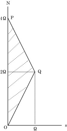
Figure 2: The inside area of OPQ denotes an area with $2s\leq N\leq 4\Omega-2s$ in Eq. (19).

In such a way, we obtained the minimum weight state in the condition $N>2s$ and the orthogonal set is given as

$$|{ss_{0},\lambda\lambda_{0};s+\lambda=\Omega}\rangle = \left({\widetilde{S}}_{+}\right)^{s+s_{0}}\left({\widetilde{\Lambda}}_{+}\right)^{\lambda+\lambda_{0}}|{s}\rangle\qquad({\rm in}\ \lambda=\Omega-s)$$ (20)

$$= \left({\widetilde{S}}_{+}\right)^{s+s_{0}}\left({\widetilde{\Lambda}}_{+}\right)^{\frac{1}{2}(N-2s)}|{s}\rangle$$

$$= \left({\widetilde{\Lambda}}_{+}\right)^{\frac{1}{2}(N-2s)}|{ss_{0}}\rangle\ .$$

Here, we used the relation (18). If paying attention only to the fact that the set $\{{\widetilde{S}}_{\pm,0}\}$ obeys the $su(2)$-algebra, we are able to obtain the eigenvalues of the Hamiltonian (5) in the space $\{|{ss_{0}}\rangle\}$ given in the relation (8). The results are not expressed in terms of $N$. In other words, there does not exist the reason why we restrict ourselves to the closed-shell system for the applicability of the Lipkin model. Any point existing in the interia of the triangle OPQ obeys the $su(2)$-Lipkin model. The point Q corresponds to the closed-shell system.

With the aim of making a connection between $({\widetilde{S}}_{0,\pm},{\widetilde{\Lambda}}_{0,\pm})$ and the minimum weight state $|{s}\rangle$ more clearly, we reform our algebra. First, we decompose ${\widetilde{S}}_{0,\pm}$ into the following two parts:

$${\widetilde{S}}_{0,\pm}={\widetilde{S}}_{0,\pm}^{(1)}+{\widetilde{S}}_{0,\pm}^{(2)}\ ,\hskip 256.0748pt$$ (21)

$${\widetilde{S}}_{0}^{(1)}=\frac{1}{2}\sum_{\mu}{}^{(1)}({\tilde{c}}_{1\mu}^{*}{\tilde{c}}_{1\mu}-{\tilde{c}}_{0\mu}^{*}{\tilde{c}}_{0\mu})\ ,\quad{\widetilde{S}}_{+}^{(1)}=\sum_{\mu}{}^{(1)}{\tilde{c}}_{1\mu}^{*}{\tilde{c}}_{0\mu}\ ,\quad{\widetilde{S}}_{-}^{(1)}=\sum_{\mu}{}^{(1)}{\tilde{c}}_{0\mu}^{*}{\tilde{c}}_{1\mu}\ ,\quad$$ (22a)

$${\widetilde{S}}_{0}^{(2)}=\frac{1}{2}\sum_{\mu}{}^{(2)}({\tilde{c}}_{1\mu}^{*}{\tilde{c}}_{1\mu}-{\tilde{c}}_{0\mu}^{*}{\tilde{c}}_{0\mu})\ ,\quad{\widetilde{S}}_{+}^{(2)}=\sum_{\mu}{}^{(2)}{\tilde{c}}_{1\mu}^{*}{\tilde{c}}_{0\mu}\ ,\quad{\widetilde{S}}_{-}^{(2)}=\sum_{\mu}{}^{(2)}{\tilde{c}}_{0\mu}^{*}{\tilde{c}}_{1\mu}\ .\quad$$ (22b)

Here, the sums $\sum_{\mu}^{(1)}$ and $\sum_{\mu}^{(2)}$ are defined as

$$\sum_{\mu}{}^{(1)}X_{\mu}=\sum_{\mu=1}^{2s}X_{\mu}\ ,\qquad\sum_{\mu}{}^{(2)}X_{\mu}=\sum_{\mu=2s+1}^{2\Omega}X_{\mu}\ .$$ (23)

They obey

$$\left[\ {\rm any\ of}\ {\widetilde{S}}_{0,\pm}^{(1)}\ ,\ {\rm any\ of}\ {\widetilde{S}}_{0,\pm}^{(2)}\ \right]=0\ .$$ (24)

The operation of ${\widetilde{S}}_{0,\pm}^{(2)}$ on $|{s}\rangle$ leads us to

$${\widetilde{S}}_{0,\pm}^{(2)}|{s}\rangle=0\ .$$ (25)

Then, we have

$${\widetilde{S}}_{-}^{(1)}|{s}\rangle=0\ ,\qquad{\widetilde{S}}_{0}^{(1)}|{s}\rangle=-s|{s}\rangle\ ,\qquad|{ss_{0}}\rangle=\left({\widetilde{S}}_{+}^{(1)}\right)^{s+s_{0}}|{s}\rangle\ .$$ (26)

For $|{ss_{0}}\rangle$, the relations (24) and (25) give us

$${\widetilde{S}}_{0,\pm}^{(2)}|{ss_{0}}\rangle=0\ .$$ (27)

The above tells us that the eigenvalue problem for $({\widetilde{S}}_{0,\pm})$ in our present model can be treated in the frame of $({\widetilde{S}}_{0,\pm}^{(1)})$. The part $({\widetilde{S}}_{0,\pm}^{(1)})$ can be rewritten in the form

$${\widetilde{S}}_{0}^{(1)}=-s+\frac{1}{2}{\tilde{n}}\ ,\qquad({\tilde{n}}=\sum_{\mu}{}^{(1)}({\tilde{a}}_{\mu}^{*}{\tilde{a}}_{\mu}+{\tilde{b}}_{\mu}^{*}{\tilde{b}}_{\mu}))$$

$${\widetilde{S}}_{+}^{(1)}=\sum_{\mu}{}^{(1)}{\tilde{a}}_{\mu}^{*}{\tilde{b}}_{\mu}^{*}\ ,\qquad{\widetilde{S}}_{-}^{(1)}=\sum_{\mu}{}^{(1)}{\tilde{b}}_{\mu}{\tilde{a}}_{\mu}\ .$$ (28)

Here, ${\tilde{a}}_{\mu}^{*}$ and ${\tilde{b}}_{\mu}^{*}$ are defined as

$${\tilde{a}}_{\mu}^{*}={\tilde{c}}_{1\mu}^{*}\ ,\qquad{\tilde{b}}_{\mu}^{*}={\tilde{c}}_{0\mu}\ .\qquad(\mu=1,\ 2,\cdots,\ 2s)$$

Needless to say, $({\widetilde{S}}_{0,\pm}^{(1)})$ obeys the $su(2)$-algebra:

$$\left[\ {\widetilde{S}}_{+}^{(1)}\ ,\ {\widetilde{S}}_{-}^{(1)}\ \right]=2{\widetilde{S}}_{0}^{(1)}\ ,\qquad\left[\ {\widetilde{S}}_{0}^{(1)}\ ,\ {\widetilde{S}}_{\pm}^{(1)}\ \right]=\pm{\widetilde{S}}_{\pm}^{(1)}\ .$$ (29)

We can see that $({\tilde{a}}_{\mu}^{*},{\tilde{a}}_{\mu})$ and $({\tilde{b}}_{\mu}^{*},{\tilde{b}}_{\mu})$ are nothing but the particle and the hole operators used in the case of the closed-shell system and if $\Omega$ used in the closed-shell system is replaced with $s$, the results are available in the case with $s<\Omega$.

We also decompose $({\widetilde{\Lambda}}_{0,\pm})$ into the following two parts :

$${\widetilde{\Lambda}}_{0,\pm}={\widetilde{\Lambda}}_{0,\pm}^{(1)}+{\widetilde{\Lambda}}_{0,\pm}^{(2)}\ ,\hskip 256.0748pt$$ (30)

$${\widetilde{\Lambda}}_{0}^{(1)}=\frac{1}{2}\sum_{\mu}{}^{(1)}({\tilde{c}}_{1\mu}^{*}{\tilde{c}}_{1\mu}+{\tilde{c}}_{0\mu}^{*}{\tilde{c}}_{0\mu})-s=\frac{1}{2}\sum_{\mu}{}^{(1)}({\tilde{a}}_{\mu}^{*}{\tilde{a}}_{\mu}-{\tilde{b}}_{\mu}^{*}{\tilde{b}}_{\mu})\ ,$$

$${\widetilde{\Lambda}}_{+}^{(1)}=\sum_{\mu}{}^{(1)}{\tilde{c}}_{1\mu}^{*}{\tilde{c}}_{0\mu}^{*}=\sum_{\mu}{}^{(1)}{\tilde{a}}_{\mu}^{*}{\tilde{b}}_{\mu}\ ,\quad{\widetilde{\Lambda}}_{-}^{(1)}=\sum_{\mu}{}^{(1)}{\tilde{c}}_{0\mu}{\tilde{c}}_{1\mu}=\sum_{\mu}{}^{(1)}{\tilde{b}}_{\mu}^{*}{\tilde{a}}_{\mu}\ ,\quad$$ (31a)

$${\widetilde{\Lambda}}_{0}^{(2)}=\frac{1}{2}\sum_{\mu}{}^{(2)}({\tilde{c}}_{1\mu}^{*}{\tilde{c}}_{1\mu}+{\tilde{c}}_{0\mu}^{*}{\tilde{c}}_{0\mu})-\lambda\ ,\quad(\lambda=\Omega-s)$$

$${\widetilde{\Lambda}}_{+}^{(2)}=\sum_{\mu}{}^{(2)}{\tilde{c}}_{1\mu}^{*}{\tilde{c}}_{0\mu}^{*}\ ,\quad{\widetilde{\Lambda}}_{-}^{(2)}=\sum_{\mu}{}^{(2)}{\tilde{c}}_{0\mu}{\tilde{c}}_{1\mu}\ .$$ (31b)

These decomposed algebras satisfy

$$\left[\ {\rm any\ of}\ {\widetilde{S}}_{0,\pm}^{(1)}\ {\rm and}\ {\widetilde{S}}_{0,\pm}^{(2)}\ ,\ {\rm any\ of}\ {\widetilde{\Lambda}}_{0,\pm}^{(1)}\ {\rm and}\ {\widetilde{\Lambda}}_{0,\pm}^{(2)}\ \right]=0\ ,$$ (32)

$${\widetilde{\Lambda}}_{0,\pm}^{(1)}|{s}\rangle=0\ ,$$ (33)

$${\widetilde{\Lambda}}_{-}^{(2)}|{s}\rangle=0\ ,\qquad{\widetilde{\Lambda}}_{0}^{(2)}|{s}\rangle=-\lambda|{s}\rangle\ .\qquad(\lambda=\Omega-s)$$ (34)

Then, by combining the above relations with the form (20), we have

$$|{ss_{0},\lambda\lambda_{0};s+\lambda=\Omega}\rangle = \left({\widetilde{\Lambda}}_{+}^{(2)}\right)^{\frac{1}{2}(N-2s)}|{ss_{0}}\rangle$$ (35)

$$= \left({\widetilde{\Lambda}}_{+}^{(2)}\right)^{\frac{1}{2}(N-2s)}\left({\widetilde{S}}_{+}^{(1)}\right)^{s+s_{0}}|{s}\rangle\ .$$

The relation (35) tells us that, in the case where the Hamiltonian (5) is investigated, at the first step, we specify the single-particle states $\mu=1,\ 2,\cdots,\ 2s$ which give us the minimum weight state $|{s}\rangle$. At the next step, we investigate the Hamiltonian (5) under appropriate method. Then, at the final step, we operate $({\widetilde{\Lambda}}_{+}^{(2)})^{\frac{1}{2}(N-2s)}$ on the eigenstates obtained at the second step and the eigenstates in the fermion number $N$ are derived. The above is our modified form of the $su(2)$-Lipkin model and, in 3, we formulate the random phase approximation (RPA) for the Hamiltonian.

3 A renewal of the conventional random phase approximation

In a way similar to that in the conventional random phase approximation (RPA), we begin our discussion with the analysis of the following equation of motion:

$$\left[\ {\widetilde{H}}\ ,\ {\widetilde{S}}_{\pm}^{(1)}\ \right]=\pm 2\epsilon{\widetilde{S}}_{\pm}^{(1)}\pm 2G\left[\ {\widetilde{S}}_{0}^{(1)}\ ,\ {\widetilde{S}}_{\mp}\ \right]_{+}\ .$$ (36)

The term $\pm 2G[{\widetilde{S}}_{0}^{(1)},{\widetilde{S}}_{\mp}]_{+}$ can be rewritten as

$$\pm 2G\left[\ {\widetilde{S}}_{0}^{(1)}\ ,\ {\widetilde{S}}_{\mp}\ \right]_{+}=\mp G\left[\ 2s-{\tilde{n}}\ ,\ {\widetilde{S}}_{\mp}^{(1)}\ \right]_{+}\mp 2G(2s-{\tilde{n}}){\widetilde{S}}_{\mp}^{(2)}\ .$$ (37)

In the case with $s=\Omega$, the term $\mp 2G(2s-{\tilde{n}}){\widetilde{S}}_{\mp}^{(2)}$ does not exist because of ${\widetilde{S}}_{\mp}={\widetilde{S}}_{\mp}^{(1)}$. And ${\tilde{n}}$ regarded as ${\tilde{n}}=0$, the relation (36) is reduced to the starting equation of the conventional RPA for the closed shell system, that is, $[{\widetilde{H}},{\widetilde{S}}_{\pm}^{(1)}]$ can be linearized for ${\widetilde{S}}_{\pm}^{(1)}$. In the case with $s<\Omega$, the term $\mp 2G(2s-{\tilde{n}}){\widetilde{S}}_{\mp}^{(2)}$ exists as the operator. However, as long as the equation of motion is investigated in the orthogonal set given in the relation (26), this term may be permitted to throw away. If we follow the above argument, our problem is to result in developing the idea how to treat ${\tilde{n}}$. Under the assumption that the change of the occupation of the single-particle states is small, it might be permitted beforehand to set up ${\tilde{n}}=0$. However, in the case where the interaction strength becomes large, the effect coming from ${\tilde{n}}$ is conjectured to be a subject of our investigation even if $s=\Omega$.

Before coming back to the main subject, we will mention some points which the Hamiltonian (5) connotes. The Hamiltonian (5) is expressed in the linear form for ${\widetilde{S}}_{0}$, $({\widetilde{S}}_{+})^{2}$ and $({\widetilde{S}}_{-})^{2}$ and, then, the eigenstates are classified in terms of the linear combinations of the even power of ${\widetilde{S}}_{+}^{(1)}$ in the states (26). Second group consists of the eigenstates expressed in terms of the linear combinations of the odd power of ${\widetilde{S}}_{+}^{(1)}$ in the states (26). Former and latter will be denoted by $|{2k})$ and $|{2k+1})$ $(k=0,1,2,\cdots)$, respectively. We regard $|{0})$ and $|{1})$ $(k=0)$ as the ground- and the first excited-state, respectively. Therefore, for the Hamiltonian (5), we have

$${\widetilde{H}}|{0})=E_{0}|{0})\ ,\qquad{\widetilde{H}}|{1})=E_{1}|{1})\ ,\qquad\omega=E_{1}-E_{0}\ (\geq 0)\ .$$ (38)

Further, without any approximation, we have the following relations for $k=0,1,2,\cdots$:

$$({1}|{\widetilde{S}}_{\pm}^{(1)}|{2k+1})=({0}|{\widetilde{S}}_{\pm}^{(1)}|{2k})=0\ ,$$ (39a)

$$({1}|{\tilde{n}}|{2k})=({0}|{\tilde{n}}|{2k+1})=0\ .$$ (39b)

With the aid of the relation $\sum_{k=0}(|{2k})({2k}|+|{2k+1})({2k+1}|)=1$ and with the use of the relation (39), we have the following :

$$({1}|{\tilde{n}}{\widetilde{S}}_{\pm}^{(1)}|{0})=\sum_{k=0}({1}|{\tilde{n}}|{2k+1})({2k+1}|{\widetilde{S}}_{\pm}^{(1)}|{0})\ ,$$ (40a)

$$({1}|{\widetilde{S}}_{\pm}^{(1)}{\tilde{n}}|{0})=\sum_{k=0}({1}|{\widetilde{S}}_{\pm}^{(1)}|{2k})({2k}|{\tilde{n}}|{0})\ .$$ (40b)

In addition to the relations (39), we introduce an approximation for terms related to $|{0})$ and $|{1})$:

$$({2k+1}|{\widetilde{S}}_{\pm}^{(1)}|{0})=({2k}|{\tilde{n}}|{0})=0\quad{\rm for}\quad k\neq 0\ .$$ (41)

Then, the relation (40) is approximated as

$$({1}|{\tilde{n}}{\widetilde{S}}_{\pm}^{(1)}|{0})=({1}|{\tilde{n}}|{1})({1}|{\widetilde{S}}_{\pm}^{(1)}|{0})=n_{1}S_{\pm}\ ,$$ (42a)

$$({1}|{\widetilde{S}}_{\pm}^{(1)}{\tilde{n}}|{0})=({1}|{\widetilde{S}}_{\pm}^{(1)}|{0})({0}|{\tilde{n}}|{0})=n_{0}S_{\pm}\ ,\qquad\qquad\qquad\qquad$$ (42b)

$$({1}|{\tilde{n}}|{1})=n_{1}\ ,\quad({0}|{\tilde{n}}|{0})=n_{0}\ ,\quad({1}|{\widetilde{S}}_{\pm}^{(1)}|{0})=S_{\pm}\ .$$ (43)

The approximate relation (42) gives us

$$({1}|[\ {\tilde{n}}\ ,\ {\widetilde{S}}_{\pm}^{(1)}\ ]_{+}|{0})=(n_{1}+n_{0})S_{\pm}\ .$$ (44)

Following the above-mentioned scheme for the approximation, we can derive the following equation from the relation (36):

$$\omega S_{\pm}=\pm 2\epsilon S_{\pm}\mp 2G(2s-n)S_{\mp}\ .$$ (45)

Here, $n$ denotes

$$n=\frac{1}{2}(n_{1}+n_{0})=n_{0}+\frac{1}{2}(n_{1}-n_{0})\ .$$ (46)

In the case with $(s=\Omega,\ n=0)$, we can see that the relation (46) is reduced to the equation derived under the conventional idea for RPA. In the conventional treatment, we have a relation to determine the absolute values of $S_{\pm}$. The relation corresponding to the conventional one is derived through the following process: With the use of the relation $({0}|[{\widetilde{S}}_{-}^{(1)},{\widetilde{S}}_{+}^{(1)}]|{0})=({0}|-2{\widetilde{S}}_{0}^{(1)}|{0})$, we have

$$\sum_{k=0}\left(({2k+1}|{\widetilde{S}}_{+}^{(1)}|{0})^{2}-({2k+1}|{\widetilde{S}}_{-}^{(1)}|{0})^{2}\right)=2s-({0}|{\tilde{n}}|{0})\ .$$ (47)

By adopting the approximation (41), the relation (47) becomes

$$(S_{+})^{2}-(S_{-})^{2}=2s-n_{0}\ .$$ (48)

In the case with $(s=\Omega,\ n_{0}=0)$, the relation (48) is written as

$$\left(S_{+}/\sqrt{2\Omega}\right)^{2}-\left(S_{-}/\sqrt{2\Omega}\right)^{2}=1\ .$$ (49)

The above is well-known formula under the name of the relation between the forward- and the backward-amplitude. The relations (45) and (48) form the basic equations of the present treatment. Needless to say, if $s=\Omega$ and $n_{0}=0$, both reduce to those in the conventional RPA. If $n_{0}$ and $n_{1}$ are given, the relations (45) and (48) give us the following results :

$$\frac{\omega}{2\epsilon}=\sqrt{1-\left(\frac{G}{\epsilon}(2s-n)\right)^{2}}\ ,\quad{\rm i.e.,}\quad\frac{G}{\epsilon}(2s-n)=\sqrt{1-\left(\frac{\omega}{2\epsilon}\right)^{2}}\ ,$$ (50)

$$(S_{\pm})^{2}=(2s-n_{0})\frac{1}{2}\left(\left(\frac{2\epsilon}{\omega}\right)\pm 1\right)\ .$$ (51)

If $s=\Omega$ and $n_{0}=n_{1}=0$, $\omega/(2\epsilon)$ can be expressed as

$$\frac{\omega}{2\epsilon}=\sqrt{1-\left(\frac{G}{\epsilon}\cdot 2\Omega\right)^{2}}\ .$$ (52)

In the case with $G\cdot 2\Omega/\epsilon=1$, $\omega/(2\epsilon)=0$ and at this point, the phase transition occurs. In our case, also the condition $G\cdot(2s-n)/\epsilon=1$ leads us $\omega/(2\epsilon)=0$. However, we can see that the above condition depends on $n$. The case $(S_{\pm})^{2}$ is also in the same situation as the above.

As was mentioned in the above, our further task is to determine $n_{0}$ and $n_{1}$ which may be functions of $\omega/(2\epsilon)$. Our first task is concerned with $n_{0}(=({0}|{\tilde{n}}|{0}))$. The idea comes from the Casimir operator (4). By calculating the expectation value $({0}|{\widetilde{\boldsymbol{S}}}^{2}|{0})(=s(s+1))$, we have

$$(2s-n_{0})^{2}+2\left(\frac{2\epsilon}{\omega}\right)(2s-n_{0})-4s(s+1)=0\ .$$ (53)

Here, $({0}|[{\widetilde{S}}_{+}^{(1)},{\widetilde{S}}_{-}^{(1)}]_{+}/2|{0})$ and $({0}|({\widetilde{S}}_{0}^{(1)})^{2}|{0})$ are approximated in the form

$$({0}|\frac{1}{2}[\ {\widetilde{S}}_{+}^{(1)},\ {\widetilde{S}}_{-}^{(1)}\ ]_{+}|{0})=\frac{1}{2}\left((S_{+})^{2}+(S_{-})^{2}\right)=\frac{1}{2}\left(\frac{2\epsilon}{\omega}\right)(2s-n_{0})\ ,$$ (54a)

$$({0}|({\widetilde{S}}_{0}^{(1)})^{2}|{0})=\left(-s+\frac{1}{2}n_{0}\right)^{2}=\frac{1}{4}(2s-n_{0})^{2}\ .$$ (54b)

Since $2s-n_{0}\geq 0$, we pick up the positive solution of the above-quadratic equation for $(2s-n_{0})$:

$$2s-n_{0}=-\frac{2\epsilon}{\omega}+\sqrt{\left(\frac{2\epsilon}{\omega}\right)^{2}+4s(s+1)}=\frac{\omega}{2\epsilon}\cdot\frac{4s(s+1)}{\sqrt{1+4s(s+1)\left(\frac{\omega}{2\epsilon}\right)^{2}}+1}\ .$$ (55)

The inverse of the above is expressed as

$$\frac{\omega}{2\epsilon}=\frac{1}{\sqrt{4s(s+1)}-(2s-n_{0})}-\frac{1}{\sqrt{4s(s+1)}+(2s-n_{0})}\ .$$ (55a)

The relation (55) will be taken up again in the relations (72), (73) and (74). We can see that the solution (55) gives us the following boundary values :

$${\rm(i)\ If}\ \omega/(2\epsilon)=1\ ,\quad 2s-n_{0}=2s\ ,\quad{\rm i.e.,}\quad n_{0}=0\ ,$$ (56a)

$${\rm(ii)\ If}\ \omega/(2\epsilon)=0\ ,\quad 2s-n_{0}=0\ ,\quad{\rm i.e.,}\quad n_{0}=2s\ .$$ (56b)

The relation (55) can be expressed as a function of $S_{-}$ :

$$n_{0}=\frac{(S_{-})^{2}}{2s+1+\sqrt{(2s+1)^{2}-4(S_{-})^{2}}}\ .$$ (57)

The above expression is approximated in the form

$$n_{0}=\frac{(S_{-})^{2}}{2(2s+1)}\ .\quad{\rm if}\quad 2s+1\gg 2(S_{-})\ ,\quad{\rm i.e.,}\quad n_{0}\ll s+\frac{1}{2}\ \ {\rm or}\ \ n_{0}\ll S_{-}\ ,$$ (58)

The form (58) may be regarded as the simplest approximate expression for $n_{0}$. As a supplementary remark, we mention the following: About sixty years ago, the effect of $n_{0}$ as the quasi-particle number was investigated in the study of the quasi-particle RPA for microscopic description of the first excited state of medium heavy even-even nuclei8 . If the formula used at that time is translated into the present model, it may be reduced to the form (58). In this case, $S_{-}/\sqrt{2s}$ plays a role of the backward amplitude in the quasi-particle RPA. Of course, the formula (58) is not applicable to the case with $n_{0}\approx 2s$.

Next, we discuss our idea for $n_{1}(=({1}|{\tilde{n}}|{1}))$. First, we notice the relation (36), which can be rewritten as follows :

$$\left[\ {\widetilde{H}}-\epsilon{\tilde{n}}\ ,\ {\widetilde{S}}_{\pm}\ \right]=\mp G\left[\ 2s-{\tilde{n}}\ ,\ {\widetilde{S}}_{\mp}\ \right]_{+}\ .$$ (59)

We discuss the case with $N=2s$ and, then, omit the superscript (1) used in 2. The relation (59) gives us

$$\left[\ {\widetilde{H}}-\epsilon{\tilde{n}}\ ,\ A{\widetilde{S}}_{+}+B{\widetilde{S}}_{-}\ \right]=-\left[\ G(2s-{\tilde{n}})\ ,\ A{\widetilde{S}}_{-}-B{\widetilde{S}}_{+}\ \right]_{+}\ .$$ (60)

Associating with the relation (60), we take up the following :

$$\left[\ {\tilde{n}}\ ,\ A{\widetilde{S}}_{+}+B{\widetilde{S}}_{-}\ \right]=2\left(A{\widetilde{S}}_{+}-B{\widetilde{S}}_{-}\right)\ .$$ (61)

For arbitrary values of $A$ and $B$, we have the relations (60) and (61). We will show that, for specific values, they are useful for our purpose. For the both sides of the relation (60), the states $|{0})$ and $|{1})$ lead us to

The left-hand side

$$= ({1}|[\ {\widetilde{H}}-\epsilon{\tilde{n}}\ ,\ A{\widetilde{S}}_{+}+B{\widetilde{S}}_{-}\ ]|{0})=\left((E_{1}-\epsilon n_{1})-(E_{0}-\epsilon n_{0})\right)(AS_{+}+BS_{-})\ ,$$

The right-hand side

$$= ({1}|-[\ G(2s-{\tilde{n}})\ ,\ A{\widetilde{S}}_{-}-B{\widetilde{S}}_{+}\ ]_{+}|{0})=-2G(2s-n)(AS_{-}-BS_{+})\ .$$ (62b)

Here, $S_{\pm}$ are shown in the relation (51) and, for the derivation of the relation (62), we adopt the approximation (42) and $n$ is given in the relation (46) ($n=(n_{1}+n_{0})/2$). For the relation (62b), we impose the condition

$$AS_{-}-BS_{+}=0\ .$$ (63)

Under this condition, the relation (62b) vanishes and $(A,B)$ is of the form

$$A=\frac{S_{+}}{(S_{+})^{2}+(S_{-})^{2}}\cdot C\ ,\qquad B=\frac{S_{-}}{(S_{+})^{2}+(S_{-})^{2}}\cdot C\ .$$ (64)

Here, $C$ denotes an arbitrary $c$-number factor $(C\neq 0$). The term $(AS_{+}+BS_{-})$ in the relation (62) is expressed as

$$AS_{+}+BS_{-}=C\neq 0\ .$$ (65)

The above consideration leads us to

$$(E_{1}-\epsilon n_{1})-(E_{0}-\epsilon n_{0})=0\ .$$ (66)

Since $E_{1}-E_{0}=\omega$, $(n_{1}-n_{0})$ is determined in the form

$$n_{1}-n_{0}=2\left(\frac{\omega}{2\epsilon}\right)\ .$$ (67)

Combining the relation (67) with (56) for the boundary values of $n_{0}$, we have

$${\rm(i)\ If}\ \ \omega/(2\epsilon)=1\ ,\ \ n_{0}=0\ \ {\rm and,\ then}\ \ n_{1}=2\ ,$$ (68a)

$${\rm(ii)\ If}\ \ \omega/(2\epsilon)=0\ ,\ \ n_{0}=2s\ \ {\rm and,\ then}\ \ n_{1}=2s\ .$$ (68b)

In order to examine the validity of the form (67), we apply our idea to the relation (61). With the use of $|{0})$ and $|{1})$, this relation is expressed in the form

$$({1}|[\ {\tilde{n}}\ ,\ A{\widetilde{S}}_{+}+B{\widetilde{S}}_{-}\ ]|{0})=2({1}|(A{\widetilde{S}}_{+}-B{\widetilde{S}}_{-})|{0})\ .$$ (69)

The above gives us

$$(n_{1}-n_{0})(AS_{+}+BS_{-})=2(AS_{+}-BS_{-})\ .$$ (70)

With the aid of the form (64), we obtain another expression for $(n_{1}-n_{0})$ :

$$n_{1}-n_{0}=2\cdot\frac{(S_{+})^{2}-(S_{-})^{2}}{(S_{+})^{2}+(S_{-})^{2}}\ .$$ (71)

Substituting the relation (51) for $(S_{\pm})^{2}$ into (71), we can see that the relation (71) is reduced to the form (67). The above argument suggests us that, for special values of $A$ and $B$, the relations (60) and (61) are compatible with each other, even if they are treated under our scheme for the approximation.

4 Discussion with numerical results

The $su(2)$-Lipkin model is, needless to say, constructed under the $su(2)$-algebra and it contains two basic parameters, $s$ and $G/\epsilon$, the numerical values of which are given from the outside. The parameter $\epsilon$ plays only a role of the measure of the energy. Therefore, the quantity such as, for example, $\omega/(2\epsilon)$, should be specified in terms of a function of $s$ and $G/\epsilon$. However, as can be seen in the relation (50) together with (55) and (67), $G/\epsilon$ is simply expressed as a function of $\omega/(2\epsilon)$. But, the inverse seems to be too complicated to give the explicit form. In this section, mainly, we will try to search the explicit form by incorporating the numerical results in the discussion.

Let us start with the discussion on $n_{0}$ and $n_{1}$. As was already mentioned, $G/\epsilon$ can be easily expressed as a function of $\omega/(2\epsilon)$. We can express $(2s-n)$ in the form

$$2s-n = 2s-n_{0}-\frac{1}{2}(n_{1}-n_{0})$$ (72)

$$= \frac{\omega}{2\epsilon}\left[\frac{4s(s+1)}{\sqrt{1+4s(s+1)\left(\frac{\omega}{2\epsilon}\right)^{2}}+1}-1\right]\ .\qquad\left(\frac{1}{2}(n_{1}-n_{0})=\frac{\omega}{2\epsilon}\right)$$

The quantity $\omega/(2\epsilon)$ changes its value in the range $0\leq\omega/(2\epsilon)\leq 1$ and we notice the following inequality :

$${\rm if}\ \ s\gg 0\ ,\qquad\frac{4s(s+1)}{\sqrt{1+4s(s+1)\left(\frac{\omega}{2\epsilon}\right)^{2}}+1}\gg 1\ .$$ (73)

For example, the case with $s=5$ and $\omega/(2\epsilon)=1/2$ gives us $120/(\sqrt{31}+1)=18.271\gg 1$. This indicates that the first term in the bracket $[\quad]$ in the relation (72) is much larger than the second, 1. Then, it may be permitted to neglect the second term, 1 and as a possible form of $(2s-n)$, we can adopt the form

$$2s-n=L\sqrt{4s(s+1)}\ .$$ (74)

Here, $L$ is defined in the form

$$L=\frac{\sqrt{4s(s+1)\left(\frac{\omega}{2\epsilon}\right)^{2}}}{\sqrt{1+4s(s+1)\left(\frac{\omega}{2\epsilon}\right)^{2}}+1}\ .$$ (75)

The above approximation corresponds to the condition $n_{1}=n_{0}$.

By substituting the relation (74) into (50), we obtain $G/\epsilon$ which is expressed in terms of $\omega/(2\epsilon)$ :

$$G/\epsilon\cdot\sqrt{4s(s+1)}L=\sqrt{1-(\omega/(2\epsilon))^{2}}\ .$$ (76)

The relation (76) gives us $\omega/(2\epsilon)$ expressed in terms of $G/\epsilon$ and $s$. If $s$ is finite, it may be easy to see that relation (76) leads us to the following two cases :

$${\rm(i)\ if}\ \ \omega/(2\epsilon)=1\ ,\quad G/\epsilon=0\ ,\quad {\rm if}\ \ G/\epsilon=0\ ,\quad\omega/(2\epsilon)=1\ ,$$

$${\rm inversely,}$$

$${\rm(ii)\ if}\ \ \omega/(2\epsilon)\rightarrow 0\ ,\quad G/\epsilon\rightarrow\infty\ , {\rm if}\ \ G/\epsilon\rightarrow\infty\ ,\quad\omega/(2\epsilon)\rightarrow 0\ .$$ (77)

In the conventional RPA, the case (i) is familiar to us, but, the case (ii) is ununderstandable. Especially, the case (ii) informs us that we cannot expect the phase transition which is well known in the conventional RPA. Therefore, it may be interesting to investigate the present RPA in parallel with the conventional RPA. For this aim, we introduce an auxiliary parameter $g/\epsilon$ which plays a role similar to that of $G/\epsilon$:

$$g/\epsilon\cdot 2s=G/\epsilon\cdot\sqrt{4s(s+1)}L\ .$$ (78)

The relation (76) can be expressed in the following form by introducing the parameter $\delta$ :

$$\delta=g/\epsilon\cdot 2s=\sqrt{1-(\omega/(2\epsilon))^{2}}\ ,\qquad{\rm i.e.,}\qquad\omega/(2\epsilon)=\sqrt{1-\delta^{2}}\ .$$ (79)

Formally, the relation (79) appears in the conventional RPA described under the interaction strength $g/\epsilon$. Associating with $\delta$, we define $\delta_{0}$ in the form

$$\delta_{0}=G/\epsilon\cdot\sqrt{4s(s+1)}\ .$$ (80)

The relations (75) and (78)$\sim$(80) give us to the following relation:

$$(\delta_{0}^{2}-\delta^{2})\sqrt{1-\delta^{2}}=\left(\frac{\delta_{0}}{\sigma}\right)\delta\ .\qquad(\sigma=\sqrt{4s(s+1)}/2)$$ (81)

With the aid of the relation (81), $\delta$ can be expressed as a function of $\delta_{0}$ and $s$. Of course, $\delta_{0}$ and $\delta$ are restricted to the condition

$${\rm(A)}\ \ 0\leq\delta_{0}\leq 1\ ,\qquad 0\leq\delta\leq\delta_{0}\ ,$$ (82a)

$${\rm(B)}\ \ 1\leq\delta_{0}\ ,\qquad\qquad 0\leq\delta\leq 1\ .$$ (82b)

Squaring both sides of the relation (81), we have

$$(\delta_{0}^{2}-\delta^{2})^{2}(1-\delta^{2})=\left(\frac{\delta_{0}}{\sigma}\right)^{2}\delta^{2}\ .$$ (83)

We can see that the relation (83) is a cubic equation for $\delta^{2}$. For example, the case with $\delta_{0}=1$ is easily solved in the exact form

$$\delta=\sqrt{1-\frac{1}{\sqrt[3]{2\sigma^{2}}}\left(\sqrt[3]{\sqrt{1+\frac{4}{27\sigma^{2}}}+1}-\sqrt[3]{\sqrt{1+\frac{4}{27\sigma^{2}}}-1}\right)}\ (=\delta^{1})\ .$$ (84)

Of course, the above obeys the condition (82). However, the process for arriving at the exact solutions in more general cases is too troublesome to treat directly the cubic equation (83). Then, we will try to find a possible approximate solutions. For this task, we use the solution (84).

Under the above preparative consideration, we will search an approximate method. The relation (81) is regarded as a quadratic equation for $\delta_{0}$ and the solution obeying the condition (82) is given by

$$\delta_{0}=\frac{\delta}{2\sigma\sqrt{1-\delta^{2}}}\left(1+\sqrt{1+\left(2\sigma\sqrt{1-\delta^{2}}\right)^{2}}\right)\ .$$ (85)

Behavior of the relation (85) is depicted in Fig.3 for the case $s=5$.

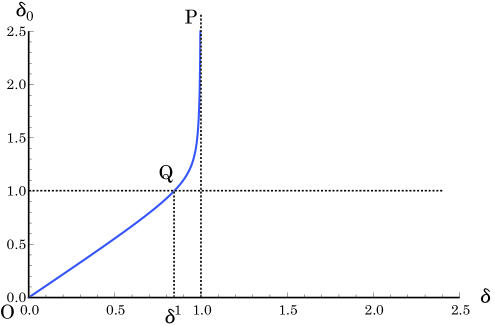
Figure 3: The exact solutions $\delta_{0}$ in Eq.(85) are depicted as a function of $\delta$.

The curve starts from the point O ($\delta=0,\ \delta_{0}=0$) under the derivative $(d\delta_{0}/d\delta)_{\delta=0}=\sqrt{(s+1)/s}$ and, via the point Q ($\delta=\delta^{1},\ \delta_{0}=1$) with the derivative $(d\delta_{0}/d\delta)_{\delta=\delta^{1}}=(2(\delta^{1})^{2}+1)/(3\delta^{1}-1)$, it gets closed to the point P ($\delta\rightarrow 1,\ \delta_{0}\rightarrow\infty$).

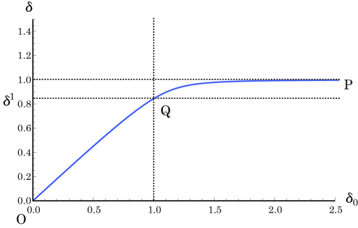
Figure 4: The exact solutions $\delta$ in Eq.(85) are depicted as a function of $\delta_{0}$.

Then, our problem is reduced to depict $\delta$ as a function of $\delta_{0}$ and it is carried out by exchanging the axis $\delta_{0}$ for the axis $\delta$ in Fig.3. In this way, we get Fig.4. For this task, the derivatives $(d\delta/d\delta_{0})_{\delta_{0}=0}=\sqrt{s/(s+1)}$ and $(d\delta/d\delta_{0})_{\delta_{0}=1}=(3\delta^{1}-1)/(2(\delta^{1})^{2}+1)$ are used and the others do not change. For an approximate expression of the curve OQP in Fig.4, we set up the form :

$$\delta=\frac{F(\delta_{0})}{\sqrt{1+F(\delta_{0})^{2}}}\ .$$ (86)

The reason why we set up the from (86) can be given as follows : Figure 4 suggests us that the curve OQP resembles the function $\sin\theta$ in the range $0\leq\theta\leq\pi$. Of course, $\theta$ may be very complicated function of $\delta_{0}$. Then, let us image a right triangle $\triangle{ABC}$ shown in Fig.5.

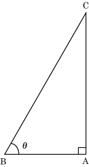
Figure 5: A right triangle $\triangle{ABC}$

In the case where the lengths of three sides of $\triangle{ABC}$ are $AB=1$, $AC=F(\delta_{0})$ and $BC=\sqrt{1+F(\delta_{0})^{2}}$, we have $\sin\theta=F(\delta_{0})/\sqrt{1+F(\delta_{0})^{2}}$. Then, following the resemblance mentioned above, it may be permitted to set up the relation (86). The above is the reason why we set up the form (86). For the relation (86), we have

$$F(\delta_{0})=\frac{\delta}{\sqrt{1-\delta^{2}}}\ ,\qquad\frac{dF(\delta_{0})}{d\delta_{0}}=\frac{\frac{d\delta}{d\delta_{0}}}{(\sqrt{1-\delta^{2}})^{3}}\ .$$ (87)

As for $F(\delta_{0})$, we adopt the following form :

$$F(\delta_{0})=a_{0}+a_{1}\delta_{0}+a_{2}(\delta_{0})^{2}+a_{3}(\delta_{0})^{3}\ .$$ (88)

Here, $a_{0}$, $a_{1}$, $a_{2}$ and $a_{3}$ denote the constants determined under the condition that $\delta$ passes the points O, Q and P with the derivatives at the points O and Q already shown. The result is as follows :

$$a_{0}=0\ ,\qquad a_{1}=\sqrt{\frac{s}{s+1}}\ ,$$

$$a_{2}=\frac{3\delta^{1}}{\sqrt{1-(\delta^{1})^{2}}}-\frac{1}{(\sqrt{1-(\delta^{1})^{2}})^{3}}\cdot\frac{3\delta^{1}-1}{2(\delta^{1})^{2}+1}-2\sqrt{\frac{s}{s+1}}\ ,$$

$$a_{3}=\frac{1}{(\sqrt{1-(\delta^{1})^{2}})^{3}}\cdot\frac{3\delta^{1}-1}{2(\delta^{1})^{2}+1}-\frac{2\delta^{1}}{\sqrt{1-(\delta^{1})^{2}}}+\sqrt{\frac{s}{s+1}}\ .$$ (89)

For the comparison, the approximate curve is shown together with the exact one in Fig.6. The agreement is quite good.

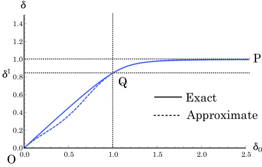
Figure 6: The comparison of the exact solutions $\delta$ in Eq.(85) and the approximate expression in Eq.(88) is depicted as a function of $\delta_{0}$.

In Fig.1, the exact and the RPA results for the first-excited energy in the $su(2)$-Lipkin model are depicted. It is ready to compare our result developed in this paper with the exact and the RPA results. In Fig.7, the first-excited energy from the ground-state energy is given in Eq.(79) with Eq.(78) with $s=5$ (dash-dotted curve) together with the RPA (dotted curve) and the exact (solid curve) results as functions of ${\overline{G}}(=G/\epsilon\cdot 2\Omega)$ which is related to $\delta_{0}$ through Eq.(80). For small $\overline{G}$, our results are close to the RPA results. However, in the region before and after $\overline{G}\approx 1$, our approximate results go away from the RPA results and approximate curve draws closer to the exact results asymptotically for $\overline{G}\gg 1$.

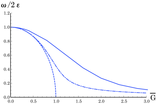
Figure 7: The first excited energies from the ground-state energy are depicted as functions of $\overline{G}=G/\epsilon\cdot 2\Omega$ for exact (solid curve), the RPA (dashed curve) results with $\Omega=5$ and our new approximate result (dash-dotted curve) in Eqs.(79) and (78) with $s=5$.

t]

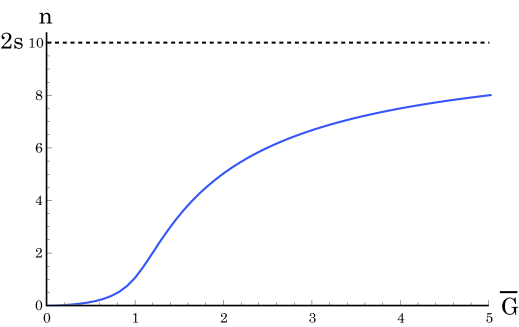
Figure 8: In the renewed RPA, $n$ is depicted as a function of ${\overline{G}}$ with $s=5$.

Here, it is interesting to see the value $n\equiv(n_{1}+n_{0})/2$ introduced in 3. As was already mentioned, if $n_{0}=n_{1}=0$, namely $n=0$, then Eq. (52) was deduced with $s=\Omega$. This result is nothing but the one derived in the conventional RPA as is depicted in Fig.7. However, in our renewed RPA, $n_{0}$ and $n_{1}$ are determined within the framework developed in 3, and as a result, $n$ is obtained. In Fig.8, the behavior of $n$ is shown numerically as a function of ${\overline{G}}$. For small $\overline{G}$ closer to zero, $n$ is nearly equal to zero. Therefore, the conventional RPA results are almost obtained as is shown in Fig.7. However, in the region before and after $\overline{G}\approx 1$, $n$ moves apart from zero. Thus, it may be good to say that our approximate results for the first-excited energy in Fig.7 go away from the conventional RPA results and our renewed RPA results draw closer to the exact ones for $\overline{G}\gg 1$.

In conclusion, it would be said that the renewed random phase approximation developed in this paper is workable beyond the conventional RPA in all the region of the interaction strength $G$ in the $su(2)$-Lipkin model.

5 Concluding remarks

In this paper, we have discussed two problems, which connote the $su(2)$-Lipkin model. Through the discussion on the first, we gave a relation among the three quantities $2\Omega$, $N$ and $s$. The result is depicted in Fig.2. Conventionally, the $su(2)$-Lipkin model has been applied only to the case with $2\Omega=N=2s$, i.e., the closed shell nuclei. However, our idea supports that we can treat this model also in the case satisfying the inequality (19). In the second, preserving the framework of the conventional RPA, we developed an idea how to investigate the term neglected in the conventional treatment. The result is depicted in Fig.7, which suggests us that we must reconsider the terminology, the “phase” used in various situations. For example, the two-level pairing model involves two phases, the non-superconductive and the superconductive phase in RPA. Figure 1 suggests us the following : The phase, which is usually interested in and may be called the normal phase, is effective in the range $0\leq G/(2\epsilon)\cdot 2s\leq 1$. In the range $1<G/(2\epsilon)\cdot 2s$, we cannot see anything. This is the result based on the conventional RPA. On the other hand, our RPA gives us the frequency $\omega/(2\epsilon)\ (>0)$ in any range of $G/(2\epsilon)\cdot 2s$ and, moreover, the result approaches the exact one. In this sense, we can treat the $su(2)$-Lipkin model only in the frame of the normal phase. The above is the second problem. If we take these two conclusions into consideration, it may be necessary to investigate another phase, which may be called the deformed phase.

With the aid of the Caylee-Klein parameters, the deformed phase in the $su(2)$-Lipkin model may be formulated. A new mean field may be constructed by the following canonical transformation from the original fermions $({\tilde{c}}_{1\mu},\ {\tilde{c}}_{0\mu}^{*})$ to the new ones $({\tilde{d}}_{1\mu},\ {\tilde{d}}_{0\mu}^{*})$ for $\mu=1,\ 2,\cdots,\ 2\Omega$ :

$$\left(\begin{array}[]{c}{\tilde{d}}_{1\mu}^{*}\\ {\tilde{d}}_{0\mu}^{*}\end{array}\right)=\left(\begin{array}[]{cc}u&-v\\ v^{*}&u^{*}\end{array}\right)\left(\begin{array}[]{c}{\tilde{c}}_{1\mu}^{*}\\ {\tilde{c}}_{0\mu}^{*}\end{array}\right)\ ,\quad{\rm i.e.,}\quad\left(\begin{array}[]{c}{\tilde{c}}_{1\mu}^{*}\\ {\tilde{c}}_{0\mu}^{*}\end{array}\right)=\left(\begin{array}[]{cc}u^{*}&v\\ -v^{*}&u\end{array}\right)\left(\begin{array}[]{c}{\tilde{d}}_{1\mu}^{*}\\ {\tilde{d}}_{0\mu}^{*}\end{array}\right)\ .$$ (102)

Here, $(u,\ v)$ and their complex conjugate are related to the Caylee-Klein parameters, the set of which is well known in the dynamics of rigid body. They satisfy the relation

$$|u|^{2}+|v|^{2}=1\ .$$ (103)

The set $(u,\ v)$ is related with the $D$-function with $j=1/2$ and in terms of the Euler angles $(\phi,\ \theta,\ \psi)$, they can be expressed as

$$u=e^{i\frac{1}{2}(\phi+\psi)}\cos\frac{\theta}{2}\ ,\qquad v=e^{i\frac{1}{2}(\phi-\psi)}\sin\frac{\theta}{2}\ .$$ (104)

The transformation (102) does not violate the basic framework of the model : After transformation, still the model consists of two single-particle levels with the degeneracy $2\Omega$ and, further, the forms of the total fermion number operator, the Casimir operator and ${\widetilde{\Lambda}}_{\pm,0}$ are unchanged. Of course, the Hamiltonian changes its form. Therefore, it may be an interesting problem to investigate the deformed phase. Finally, we stress that the $su(2)$-Lipkin model still connotes the problem to give the solution.

References

(1)
K. Sawada, Phys. Rev. 106, 372 (1957).
K. Sawada, K. A. Brueckner, N. Fukuda and R. Brout, Phys. Rev. 108, 507 (1957).
(2)
S. Takagi, Prog. Theor. Phys. 21, 174 (1959).
K. Ikeda, M. Kobayasi, T. Marumori, T. Shiozaki and S. Takagi, Prog. Theor. Phys. 22, 663 (1959).
S. Hatano, Prog. Theor. Phys. 24, 412 (1960).
G. E. Brown, J. A. Evans and D. J. Thouless, Nucl. Phys. 24,1 (1961).
(3)
R. Arvieu and M. Vénéroni, Compt. Rend. 250, 992 (1960).
M. Baranger, Phys. Rev. 120, 957 (1960).
T. Marumori, Prog. Theor. Phys. 24, 331 (1960).
(4)
H. J. Lipkin, N. Meshkov and A. Glick, Nucl. Phys. 62, 188 (1965).
(5)
Y. Tsue, C. Providência, J. da Providência and M. Yamamura, Prog. Theor. Phys. 127, 117; 303, (2012).
Y. Tsue, C. Providência, J. da Providência and M. Yamamura, Prog. Theor. Exp. Phys. 2016, 083D03; 083D04, (2016):
ibid. 2017, 081D01 (2017).
(6)
A. Klein and E. R. Marshalek, Rev. Mod. Phys. 63, 375 (1991).
(7)
J. Terasaki, A. Smetana, F. Šimkovic and M. I. Krivoruchenko, Int. J. Mod. Phys. E 26, 1750062 (2017).
(8)
J. da Providência, Nucl. Phys. 61, 87 (1965).
(9)
J. da Providência, Nucl. Phys. 83, 209 (1966).
(10)
J. da Providência, Nucl. Phys. A 108, 589 (1968).
(11)
J. da Providência, Nucl. Phys. A157, 358 (1970).
(12)
D. M. Brink and A. Weiguny, Phys Lett. 26B, 494 (1968).
D. M. Brink and A. Weiguny, Nucl. Phys. A120, 59 (1968).
H. Ui and L. C. Biedenharn, Phys. Lett. 26B, 608 (1968).
Chun Wa Wong, Nucl. Phys. A417, 545 (1970).
(13)
K. Hara, Prog. Theor. Phys. 32, 88 (1964).
K. Ikeda, T. Udagawa and H. Yamaura, Prog. Theor. Phys. 33, 22 (1965).
Y. Miyanishi and M. Yamamura, Prog. Theor. Phys. 38, 332 (1967).