Dependence of NLRs sizes on [O iii]  luminosity in low redshift AGN with double-peaked broad Balmer emission lines

Abstract

In the manuscript, the simple but interesting results are reported on the upper limits of NLRs sizes of a small sample of 38 low redshift ($z<0.1$) AGN with double-peaked broad emission lines (double-peaked BLAGN), in order to check whether the NLRs sizes in type-1 AGN and type-2 AGN obey the similar empirical dependence on [O iii]  luminosity. In order to correct the inclination effects on projected NLRs sizes of type-1 AGN, the accretion disk origin is commonly applied to describe the double-peaked broad H$\alpha$ leading to the determined inclination angles of central disk-like BLRs of the 38 double-peaked BLAGN. Then, considering the fixed SDSS fiber radius, the upper limits of NLRs sizes of the 38 double-peaked BLAGN can be estimated. Meanwhile, the strong linear correlation between continuum luminosity and [O iii]  luminosity is applied to confirm that the [O iii]  emissions of the 38 double-peaked BLAGN are totally covered in the SDSS fibers. Considering the reddening corrected measured [O iii]  luminosity, the upper limits of NLRs sizes of the 38 double-peaked BLAGN are within the 99.9999% confidence interval of the expected results from the empirical relation between NLRs sizes and [O iii]  luminosity in the type-2 AGN. In the current stage, there are no clues to challenge the Unified model of AGN, through the space properties of NLRs.

1 Introduction

Strong [O iii]  emission lines are fundamental characteristics of both broad line Active Galactic Nuclei (type-1 AGN) and narrow line AGN (type-2 AGN). Under the current framework of the preferred being-improved Unified Model (Antouncci, 1993; Netzer, 2015), type-1 AGN and type-2 AGN have totally the same central structures of narrow emission line regions (NLRs) and broad emission line regions (BLRs) (the two essential structures of AGN), but the BLRs are seriously obscured by central dust torus leading to no apparent broad optical emission lines detected in type-2 AGN. The well detected polarized broad emission lines in type-2 AGN, such as the results well discussed in Antonucci & Miller (1985); Tran (2001, 2003); Nagao et al. (2004); Cardamone et al. (2007); Shi et al. (2010); Barth et al. (2014); Pons & Watson (2016); Savic et al. (2018), provide robust evidence to strongly support the hidden BLRs in type-2 AGN. Certainly, there is one precious subclass of true type-2 AGN: type-2 AGN without hidden BLRs. More recent arguments on the very existence of true type-2 AGN can be found in Bianchi et al. (2019); Zhang et al. (2021). We mainly focus on properties of NLRs sizes of AGN, therefore, we do not discuss true type-2 AGN in the manuscript.

Basic physical sizes of NLRs in type-2 AGN and of BLRs in type-1 AGN have been well known. Sizes of BLRs ($R_{BLRs}$ distances between BLRs to central black hole (BH)) can be well determined by the well-known reverberation mapping technique (Blandford & McKee, 1982), through long-term variabilities of broad emission lines and continuum emissions. Peterson et al. (2004) have reported the measured sizes of BLRs in the sample of nearby broad line AGN (BLAGN) in the AGNWATCH project (see dozens of published papers listed in the project). Kaspi et al. (2000, 2005) have reported the measured sizes of BLRs of nearby 17 quasars. Bentz et al. (2010); Barth et al. (2015); Williams et al. (2018) have reported the measured sizes of BLRs in the sample of nearby Seyfert galaxies in the LAMP project. Wang et al. (2014); Du et al. (2016) have reported the measured sizes of BLRs in the sample of nearby Seyferts with high accretion rates. Shen et al. (2015); Grier et al. (2017) have reported the measured sizes of BLRs in the sample of SDSS QSOs. The reverberation mapping technique determined sizes of BLRs leads to the well accepted empirical relation between $R_{BLRs}$ and continuum luminosity of broad line AGN discussed and shown in Kaspi et al. (2000, 2005); Bentz et al. (2013).

Unlike the measurements of BLRs sizes in type-1 AGN, longer extended structures of NLRs indicate reverberation mapping technique can not be applied to measure NLRs sizes ($R_{NLRs}$) due to no variabilities in narrow emission lines (expected variability timescale around hundreds of years). However, in some nearby type-2 AGN or nearby high luminosity type-2 QSOs, the NLRs sizes have been well determined by properties of spatial resolved [O iii]  emission images, such as the measured NLRs sizes in Seyfert 2 galaxy NGC1386 in Bennert et al. (2006a), in the small sample of in Seyfert-2 galaxies in Bennert et al. (2006b), in the sample of 15 obscured QSOs in Greene et al. (2011), in the radio quiet type-2 QSOs in Liu et al. (2013a, b), in the luminous obscured QSOs in Hainline et al. (2013, 2014), in the obscured QSOs in Fischer et al. (2018), etc. Then, based on the measured sizes of NLRs, there is one empirical R-L relation between NLRs sizes and [O iii]  luminosity ($L_{[O~{}\textsc{iii}]}$) (in the manuscript, the R-L relation is for the relation on NLRs sizes, unless with specific statements) discussed and shown in Liu et al. (2013a); Hainline et al. (2013, 2014); Fischer et al. (2018); Dempsey & Zakamska (2018),

$$\begin{split}\log(\frac{R_{NLRs}}{\rm pc})=&(0.250\pm 0.018)\times\log(\frac{L_{[O~{}\textsc{iii}]}}{\rm 10^{42}erg/s})\\ &+(3.746\pm 0.028)\end{split}$$ (1)

, especially for AGN with 8$\mu$m luminosity smaller than $10^{45}{\rm erg/s}$ as discussed in Hainline et al. (2013); Dempsey & Zakamska (2018). In order to explain the R-L relation of NLRs, Liu et al. (2013a) have proposed a model of [O iii]  emission clumpy nebulae in which clouds that produce line emission transition from being ionization-bounded at small distances from central power source to being matter-bounded in the outer parts of the clumpy nebulae. Similar model was also discussed in Greene et al. (2011). More recently, Dempsey & Zakamska (2018) have re-constructed the R-L relation of NLRs by the proposed model that the NLRs as a collection of clouds in pressure equilibrium with the ionizing radiation.

Actually, NLRs sizes in type-1 AGN are hardly to be measured mainly due to inclination effects, although Bennert et al. (2002); Schmitt et al. (2003a, b) have reported NLRs sizes in several nearby broad line AGN. However, the measured NLRs sizes of the type-1 AGN in the literature, such as the results in Schmitt et al. (2003b), are about 1-2 magnitudes smaller than the expected results from the empirical relation between NLRs sizes and [O iii]  luminosity in the type-2 AGN in Liu et al. (2013a), which could be mainly due to inclination effects and/or quite shallow observations. Therefore, NLRs sizes of type-1 AGN in Schmitt et al. (2003b) are not considered in the manuscript. However, there is one subclass of type-1 AGN, the broad line AGN with double-peaked broad low-ionization emission lines (called as double-peaked BLAGN) of which inclination angles can be reasonably estimated, accepted accretion disk origin of the double-peaked broad emission lines as well discussed in Chen & Halpern (1989); Eracleous et al. (1995); Storchi-Bergmann et al. (2003); Strateva et al. (2003); Flohic & Eracleous (2008); Storchi-Bergmann et al. (2017), etc. In the manuscript, considering the fixed diameter of SDSS fibers, upper limits of NLRs sizes in low redshift double-peaked BLAGN in SDSS can be well estimated, which will be applied to test the R-L empirical relation of NLRs in type-1 AGN. The tests can provide further clues on whether there are difference of spatial distances of NLRs between type-1 AGN and type-2 AGN, to challenge or to support the Unified model of AGN, which is the main objective of the manuscript. Section 2 presents our hypotheses on estimating sizes of NLRs of double-peaked BLAGN. Section 3 shows our main sample of double-peaked BLAGN. Section 4 shows our main results and necessary discussions. Section 5 gives our final summaries and conclusions. We have adopted the cosmological parameters $H_{0}=70{\rm km\cdot s}^{-1}{\rm Mpc}^{-1}$, $\Omega_{\Lambda}=0.7$ and $\Omega_{\rm m}=0.3$ in the manuscript.

Figure 1: SDSS spectra of the 38 low redshift double-peaked BLAGN (marked with information of PLATE-MJD-FIBERID, and listed in the order shown in Table 1) and the best descriptions to the stellar lights by the SSP method. In each panel (except the ones without apparent stellar lights), solid dark green line shows the SDSS spectrum, solid red line shows the best descriptions to the SDSS spectrum with the emission lines being masked out, solid purple line shows the SSP method determined stellar lights, and solid blue line shows the determined power law AGN continuum emissions. In each panel, from left to right, the vertical red lines mark the following emission features masked out, including [O ii]$\lambda 3727$Å , H$\theta$, H$\eta$, [Ne iii]$\lambda 3869$Å, He i$\lambda 3891$Å, Calcium K line, [Ne iii]$\lambda 3968$Å, Calcium H line, [S ii]$\lambda 4070$Å, H$\delta$, H$\gamma$, [O iii]$\lambda 4364$Å, He i$\lambda 5877$Å and [O i]$\lambda 6300,6363$Å, respectively, and the area filled by red lines around 5000Å shows the region masked out including the emission features of probable optical Fe ii lines, broad and narrow H$\beta$ and [O iii] doublet, and the area filled by red lines around 6550Å shows the region masked out including the emission features of broad and narrow H$\alpha$, [N ii] and [S ii] doublets.Bottom region of each panel shows the residuals calculated by SDSS spectrum minus sum of the stellar lights and the power law continuum emissions, for the object with apparent stellar lights. In order to show clearly spectral features and features of stellar lights, the Y-axis is in logarithmic coordinate for the plots in top region of each panel.

Figure 1: –continued.

Figure 1: –continued.

2 Main Hypotheses on estimating upper limits of sizes of NLRs of double-peaked BLAGN

In order to explain the double-peaked broad emission lines of AGN, besides the accretion disk origin (Chen & Halpern, 1989; Eracleous et al., 1995; Storchi-Bergmann et al., 2017), the theoretical binary black hole model (BBH model) (Begelman et al., 1980; Di Matteo et al., 2005; Pfister et al., 2017; Sayeb et al., 2021) has been well proposed, such as the BBH model once applied to describe variability properties of the double-peaked broad Balmer lines of 3C390.3 in Gaskell (1996) and theoretical BBH model applied to generate double-peaked broad lines in Shen & Loeb (2010), etc. Once accepted the BBH model to explain the double-peaked broad emission lines, quasi-periodic oscillations (QPOs) could be expected, such as the well discussed in Graham et al. (2015a, b); Zheng et al. (2016); Liao et al. (2021); Zhang (2022) with QPOs signs applied to detect candidates for BBH systems. However, through the study of long-term variabilities of double-peaked BLAGN in Eracleous et al. (1997); Shapovalova et al. (2001); Storchi-Bergmann et al. (2003); Lewis, Eracleous & Storchi-Bergmann (2010); Zhang (2013); Zhang & Feng (2017), quite few QPOs can be commonly detected in long term variabilities of double-peaked BLAGN. Moreover, among the 38 collected low-redshift double-peaked BLAGN in our final sample in the following section, 37 double-peaked BLAGN have their long-term light curves collected from CSS (Catalina Sky Survey) (Drake et al., 2009). Long-term variability analysis of our sources does not show any QPOs signs as shown in section 4. Therefore, in the manuscript, the accretion disk origin has been well accepted to explain the double-peaked broad emission lines, and no further discussions are shown on the BBH model.

There are different kinds of relativistic accretion disk models in the literature, such as the circular accretion disk model in Chen & Halpern (1989), the improved elliptical accretion disk model in Eracleous et al. (1995), the model of circular disk with spiral arms in Storchi-Bergmann et al. (2003), a warped accretion disk model in Hartnoll & Blackman (2000), and a stochastically perturbed accretion disk model in Flohic & Eracleous (2008), etc. Here, the elliptical accretion disk model (without contributions of subtle structures) well discussed in Eracleous et al. (1995) is preferred, because the model can be applied to explain almost all observational double-peaked features of the double-peaked BLAGN in our sample. There are seven model parameters in the elliptical accretion disk model, inner boundary $r_{0}$ and out boundary $r_{1}$ in the units of $R_{G}$ (Schwarzschild radius), inclination angle $i$ of disk-like BLRs, eccentricity $e$, orientation angle $\phi_{0}$ of elliptical rings, local broadening velocity $\sigma_{L}$, line emissivity slope $q$ ($f_{r}~{}\propto~{}r^{-q}$). Meanwhile, we have also applied the very familiar elliptical accretion disk model, see our studies on double-peaked lines in Zhang et al. (2005); Zhang (2013a, 2015); Zhang et al. (2019). More detailed descriptions on the applied elliptical accretion disk model can be found in Eracleous et al. (1995); Storchi-Bergmann et al. (2003); Strateva et al. (2003), and there are no further discussions on the elliptical accretion disk model in the manuscript. Then, the elliptical accretion disk model can be well applied to describe double-peaked broad emission lines, leading to the well determined inclination angle $\sin(i)$ of central accretion disk.

Considering the SDSS fiber diameter of 3 arcseconds (2 arcseconds for eBOSS, the Extended Baryon Oscillation Spectroscopic Survey (detailed descriptions can be found in the web) as the projected space distance $D_{s}$ in units of $pc$, and considering the inclination angle $\sin(i)$ determined by the elliptical accretion disk model, the upper limits of sizes of the [O iii]  emission regions, as the upper limits of NLRs sizes $R_{NLRs,u}$, should be estimated as

$$R_{NLRs,u}=\frac{D_{s}}{sin(i)}$$ (2)

.

Before the end of the section, it is interesting to check whether the equation above can be reasonably applied to estimate upper limits of NLRs sizes of AGN. For the 14 obscured quasars well discussed in Liu et al. (2013a), their upper limits of NLRs sizes can be estimated as SDSS fiber radius of 1.5 arcseconds. Here, for the obscured quasars (type-2 quasar), we simply accepted $sin(i)\sim 1$. Due to the high redshift around 0.5 of the 14 obscured quasars, their upper limits of NLRs sizes are about $2.06\times 10^{4}pc$, quite larger than their measured NLRs sizes in Liu et al. (2013a), indicating the method to estimate upper limits of NLRs sizes are reasonable to some extent.

3 Sample of the double-peaked BLAGN

In the manuscript, we mainly consider the low redshift double-peaked BLAGN with redshift smaller than 0.1 by the following main reason. For redshift at 0.1 (distance about 460.3Mpc), the corresponding space distance of the SDSS fiber radius (1.5 arcseconds) is about $3350{\rm pc}$ ($10^{3.53}{\rm pc}$), similar as the mean value about $10^{3.5}{\rm pc}$ of the measured NLRs sizes of type-2 QSOs in Liu et al. (2013a); Hainline et al. (2013); Fischer et al. (2018). For objects with redshift quite larger than 0.1, the corresponding space distance by the SDSS fibers should be clearly larger than the expected sizes of NLRs, indicating that it is meaningless to check properties of upper limits of NLRs sizes of type-1 objects with redshift quite larger than 0.1.

We collect double-peaked BLAGN with redshift smaller than 0.1 as follows. On the one hand, there are 4 double-peaked BLAGN with redshift smaller than 0.1 in the sample of double-peaked BLAGN listed in Strateva et al. (2003), SDSS 0721-52228-0600 (SDSS PLATE-MJD-FIBERID), SDSS 0725-52258-0510, SDSS 0746-52238-0409 and SDSS 6139-56192-0440 (spectrum from eBOSS with fiber radius 1arcseconds). On the other hand, the other 11 appropriate double-peaked BLAGN are collected by the following two steps. First, all the 1752 SDSS QSOs with signal-to-noise larger than 10 and redshift smaller than 0.1 are firstly collected from SDSS DR16 (Data Release 16 (Ahumada et al., 2020)) by the following SQL query

⬇

SELECT

plate, fiberid, mjd

FROM SpecObjall

WHERE

class = ’QSO’ and z < 0.1

and zwarning = 0 and snmedian > 10

. Second, emission lines of all the 1752 SDSS QSOs are measured after host contributions are determined, as what are discussed in the following section. And then, we mainly check the QSOs with the broad H$\alpha$ described by more than 2 broad Gaussian components one by one by eyes, and collect 11 double-peaked BLAGN based on the criterion that there is at least one apparent hump included in the red-side or blue-side of broad H$\alpha$. Unfortunately, it is hard to provide a standard criterion which can be well described by a formula or formulas to collect candidates of AGN with double-peaked broad emission lines, therefore, the collected double-peaked BLAGN are identified by eyes.

Besides the double-peaked BLAGN collected from SDSS quasars in DR16, there is a sample of candidates of double-peaked BLAGN collected from SDSS main galaxies and reported in Liu et al. (2019). Then, based on the same criteria of $z~{}<~{}0.1$ and signal-to-noise of SDSS spectrum larger than 10, there are 106 candidates of double-peaked BLAGN collected from the sample of Liu et al. (2019) with the flag MULTI_PEAK=2. Furthermore, two additional criteria are accepted to collect double-peaked BLAGN from the sample of Liu et al. (2019). On the one hand, there should be apparent narrow Balmer emission lines detected in the SDSS spectra, in order to correct reddening effects on observed [O iii] emission intensities. On the other hand, there should be apparent both broad H$\alpha$ and broad H$\beta$ detected in the SDSS spectra, in order to ignore seriously obscurations on central BLRs, and in order to confirm the collected double-peaked BLAGN from SDSS main galaxies are also type-1 AGN (not type-1.5 nor type-1.9 AGN) totally similar as the double-peaked BLAGN (type-1 AGN) collected from SDSS quasars. Based on the two additional criteria, 23 double-peaked BLAGN are finally collected from the sample of Liu et al. (2019). In the following section, two examples are shown on an AGN with double-peaked broad H$\alpha$ but no apparent narrow Balmer emission lines, and on an AGN with only double-peaked broad H$\alpha$ but no apparent double-peaked broad H$\beta$, from the sample of Liu et al. (2019), after subtractions of host galaxy contributions from the SDSS spectra. Finally, there are 38 double-peaked BLAGN with redshift smaller than 0.1 included in our sample, 15 double-peaked BLAGN collected from SDSS quasars and 23 double-peaked BLAGN collected from the sample of Liu et al. (2019). The basic information of the 38 double-peaked BLAGN are listed in Table 1, including the PLATE-MJD-FIBERID, redshift, etc.

Figure 2: The best fitting results to the emission lines around H$\beta$ (panels in the first and the third column) and around H$\alpha$ (panels in the second and the fourth column) by multiple Gaussian functions. In each panel, solid line in dark green shows the line spectrum after subtractions of the contributions of stellar lights, solid red line shows the best fitting results by multiple Gaussian components plus a power law component, solid blue lines show the determined broad Gaussian components in the Balmer line, solid green line and solid cyan line (if there was) show the determined narrow and extended components in the Balmer line, and dashed blue line shows the determined power law component. In each panel in the first and the third column, solid pink line and solid purple line show the determined narrow and extended components in [O iii] doublet. In each panel in the second and the fourth column, solid lines in pink show the determined [O i] doublet including both narrow and extended components, solid purple lines show the determined [N ii] doublet, solid lines in magenta show the determined [S ii] doublet. In the panels for best fitting results around H$\beta$ of SDSS 0966-52642-0499, SDSS 2123-53793-0443 and SDSS 2783-54524-0517, dashed cyan lines show the determined optical Fe ii emission features. Bottom region of each panel shows the residuals calculated by line spectrum minus the best fitting results. In order to show clearly spectral broad emission line features, the Y-axis is in logarithmic coordinate for the plots in top region of each panel.

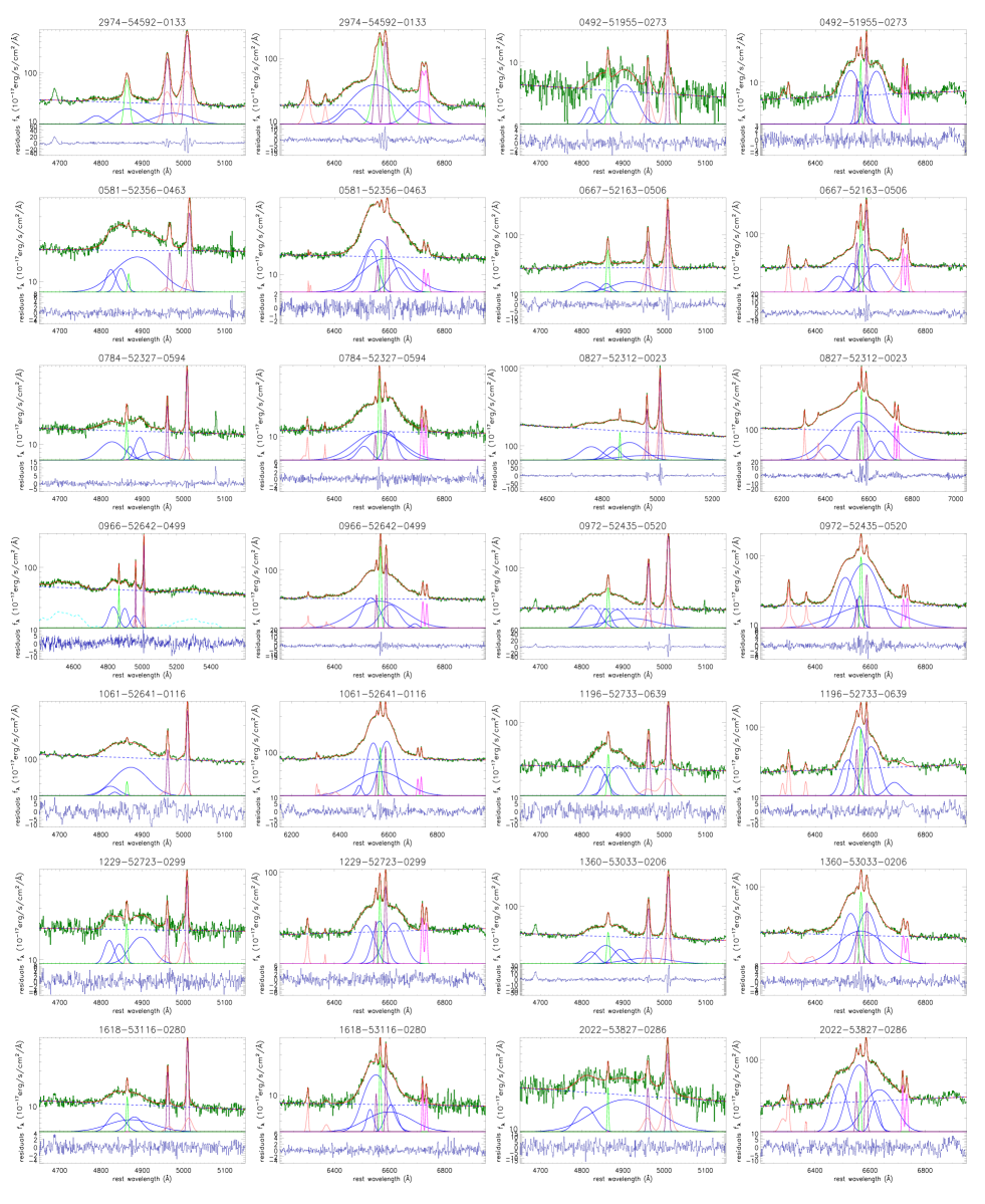
Figure 2: –continued.

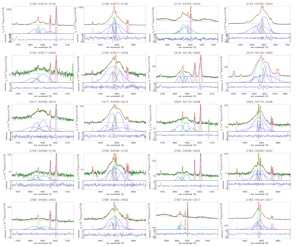
Figure 2: –continued.

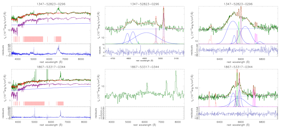
Figure 3: Two examples on the BLAGN with double-peaked broad H$\alpha$ identified in Liu et al. (2019), but without apparent narrow H$\beta$ in SDSS 1347-52823-0296 (top panels), without apparent broad H$\beta$ in SDSS 1867-53317-0344 (bottom panels). Each left panel shows the SDSS spectrum and the SSP method determined host galaxy contributions, symbols and line style have the same meanings as those in Figure 1. Middle and right panels show the best descriptions to the emission lines around H$\beta$ and around H$\alpha$, symbols and line style have the same meanings as those in Figure 2. Here, due to lack of apparent broad H$\beta$, there are no fitting results shown in bottom middle panel.

4 Main procedures, Main results and Main discussions

For the 38 double-peaked BLAGN, the SDSS spectra are shown in Figure 1. It is clear that there are apparent stellar lights included in the spectra of 30 double-peaked BLAGN. The stellar lights should be firstly determined, in order to find more accurate line profiles of emission lines, especially of the narrow emission lines. In the manuscript, the well accepted SSP (Simple Stellar Population) method is applied. Detailed discussions and descriptions on the SSP method can be found in Bruzual & Charlot (2003); Kauffmann et al. (2003); Cid Fernandes et al. (2005), here we do not show them any more. Similar as what we have previously done in Zhang (2014); Zhang et al. (2016, 2019); Zhang (2021a, b) to describe the stellar lights included in SDSS spectra of broad line AGN, we here exploit a power law component $\alpha\times\lambda^{\beta}$ applied to describe the AGN continuum emissions and the 39 simple stellar population templates from the Bruzual & Charlot (2003) which include the population age from 5Myr to 12Gyr, with three solar metallicities (Z = 0.008, 0.05, 0.02). Then through the Levenberg-Marquardt least-squares minimization method applied to the SDSS spectra with both narrow and broad emission lines being masked out, host galaxy contributions and the intrinsic AGN power law continuum components in the SDSS spectra can be clearly determined. Here, when the SSP method is applied, the emission lines are being masked out by line width about 400${\rm km/s}$ at zero intensity, and the broad H$\alpha$, H$\beta$ and H$\gamma$ are being masked out by line width about 3000${\rm km/s}$ at zero intensity, and the probable optical Fe ii emission lines (Kovacevic-Dojcinovic et al., 2010) are being masked out with rest wavelength range from 4400Å  to 5600Å. Meanwhile, when the model functions are applied, there are 42 model parameters, 39 strengthen factors with zero as the starting values for the 39 SSPs, the broadening velocity with ${\rm 100km~{}s^{-1}}$ as the starting value, $\alpha$ and $\beta$ for the power law component with zero as the starting values. The SSP method determined stellar lights and corresponding residuals are clearly shown in Figure 1 for the 30 double-peaked BLAGN with apparent stellar lights. Here, the residuals shown in Figure 1 are calculated by SDSS spectrum minus sum of the stellar lights and the power law continuum emissions. The values of $\chi^{2}$ (summed squared residuals divided by degree of freedom) are listed in Table 1 for the best fitting results to the SDSS spectra with emission lines being masked out.

Before subtracting the stellar lights from the SDSS spectra, one point is noted. Among the 30 double-peaked BLAGN of which SDSS spectra include apparent contributions of stellar lights, there are six objects, SDSS 1393-52824-0216, SDSS 1624-53386-0032, SDSS 0492-51955-0273, SDSS 1229-52723-0299, SDSS 2022-53827-0286 and SDSS 2419-54139-0083, of which intrinsic AGN continuum emissions are determined and described by red power law functions ($\beta~{}\geq~{}0$) not by commonly blue power law functions ($\beta~{}<~{}0$). The red power law AGN continuum emissions are probably due to intrinsic reddening effects of host galaxies and/or central high density clouds. The intrinsic reddening could have effects on strengths of broad emission lines but have few effects on line profiles of broad emission lines. Whereas, the main consider parameter of inclination angle is determined through properties of double-peaked line profiles. Therefore, although in the procedure above to determine contributions of stellar lights without considerations of intrinsic reddening effects, there are few effects on our final results on the upper limits of NLRs sizes of the collected low redshift double-peaked BLAGN.

After subtractions of the contributions of stellar lights, the emission lines are modeled by multiple Gaussian functions, in order to obtain more accurate line parameters (or line profiles) of both narrow and broad emission lines. Similar as what we have recently done in Zhang (2021a), the following model functions are applied to describe the emission lines around H$\alpha$ within rest wavelength range from 6250Å  to 6850Å, four broad Gaussian functions (second moment larger than 400${\rm km/s}$) applied to describe the broad H$\alpha$, one narrow Gaussian function (second moment smaller than 400${\rm km/s}$) plus one broad Gaussian function applied to describe the narrow and extended (if there was) components of narrow H$\alpha$, two narrow Gaussian functions applied to describe the [N ii] doublet, two narrow Gaussian functions applied to describe the [S ii] doublet, and two narrow plus two broad Gaussian functions applied to describe the [O i] doublet and a power law component $\alpha_{1}\times\lambda^{\beta}_{1}$ applied to describe the AGN continuum emissions underneath the emission lines around H$\alpha$. Similarly, the following model functions are applied to describe the emission lines around H$\beta$ within rest wavelength range from 4650Å  to 5250Å, four broad Gaussian functions applied to describe the broad H$\beta$, one narrow plus one broad Gaussian functions applied to describe the narrow and extended components of narrow H$\beta$, two narrow plus two broad Gaussian functions applied to describe the [O iii] doublet and a power law component $\alpha_{2}\times\lambda^{\beta}_{2}$ applied to describe the intrinsic AGN continuum emissions underneath the emission lines around H$\beta$.

When the model functions are applied to describe emission lines around H$\alpha$, there are 44 model parameters, 12 model parameters from the 4 broad Gaussian components (three model parameters for each broad Gaussian component, central wavelength $\lambda_{0b,~{}i}$, second moment $\sigma_{b,~{}i}$ and line flux $f_{b,~{}i}$) for the broad H$\alpha$, 21 model parameters from the 7 narrow Gaussian components (three model parameters for each Gaussian component, central wavelength $\lambda_{0n,~{}j}$, second moment $\sigma_{n,~{}j}$ and line flux $f_{n,~{}j}$), 9 model parameters from the three extended components of narrow H$\alpha$ and [O i] doublet ($\lambda_{0e,~{}k}$, $\sigma_{e,~{}k}$ and $f_{e,~{}k}$) and 2 model parameters $\alpha_{1}$ and $\beta_{1}$ for the power law component. The restrictions on the 44 model parameters are as follows. First, all broad and narrow Gaussian components have line fluxes not smaller than zero $f_{b,~{}i}~{}\geq~{}0~{}(i=1,~{}\dots,~{}4)$, $f_{n,~{}j}~{}\geq~{}0~{}(j=1,~{}\dots,~{}7)$ and $f_{e,~{}k}~{}\geq~{}0~{}(k=1,~{}\dots,~{}3)$, and have zero as the starting values of $f_{b,~{}i}$, $f_{n~{},j}$ and $f_{e,~{}k}$. Second, the 7 narrow Gaussian components have second moments smaller than 400${\rm km/s}$, $0~{}<~{}\sigma_{n,~{}j}~{}\leq~{}400{\rm km/s}~{}(j=1,~{}\dots,~{}7)$, and have 100${\rm km/s}$ as the starting values. Third, the 4 broad Gaussian components in broad Balmer lines have second moments larger than 400${\rm km/s}$, $\sigma_{b,~{}i}~{}\geq~{}400{\rm km/s}~{}(i=1,~{}\dots,~{}4)$, and have 1000${\rm km/s}$ as the starting values. Fourth, the 3 broad Gaussian components for the extended emission components in narrow emission lines have second moments larger than those of the corresponding narrow components, but have 600${\rm km/s}$ as the starting values. Fifth, the 7 narrow Gaussian components have central wavelengths in units of Å  to be within the range $\lambda_{0T,~{}j}-15\textsc{\AA}~{}\leq~{}\lambda_{0n,~{}j}~{}\leq~{}\lambda_{0T,~{}j}+15\textsc{\AA}$ with $\lambda_{0T,~{}j}~{}(j=1,~{}\dots,~{}7)$ as the theoretical vacuum rest wavelength of the emission component, and have $\lambda_{0T,~{}j}$ as the starting values. Sixth, the 3 broad Gaussian functions for the extended emission components have central wavelengths in units of Å  to be within the range $\lambda_{0T,~{}k}-30\textsc{\AA}~{}\leq~{}\lambda_{0e,~{}k}~{}\leq~{}\lambda_{0T,~{}k}+30\textsc{\AA}$ with $\lambda_{0T,~{}k}~{}(k=1,~{}\dots,~{}3)$ as the theoretical vacuum rest wavelength of the emission component, and have $\lambda_{0T,~{}k}$ as the starting values. Seventh, the 4 broad Gaussian components for broad H$\alpha$ have central wavelengths in units of Å  to be within the range $6450\textsc{\AA}~{}\leq~{}\lambda_{0b,~{}i}~{}\leq~{}6650\textsc{\AA}$, and have 6490Å, 6520Å, 6580Å, 6620Å  as the starting values. Eighth, $\alpha_{1}$ and $\beta_{1}$ are restricted by $\alpha_{1}~{}\geq~{}0$ and $-5~{}\leq~{}\beta_{1}~{}\leq~{}1$. Ninth, the flux ratio of [N ii] doublet is fixed to the theoretical values of 3. Tenth, the Gaussian components from each doublet have the same redshift and the same second moment.

Similar restrictions are applied to the 32 model parameters, when the model functions are applied to describe the emission lines around H$\beta$. There are 12 model parameters from the 4 broad Gaussian components ($\lambda_{0b,~{}i}$, $\sigma_{b,~{}i}$, $f_{b,~{}i}$, $i=1,~{}\dots,~{}4$) for the broad H$\beta$, 9 model parameters from the 3 narrow Gaussian components ($\lambda_{0n,~{}j}$, $\sigma_{n,~{}j}$, $f_{n,~{}j}$), 9 model parameters from the three extended components of narrow H$\beta$ and [O iii] doublet ($\lambda_{0e,~{}k}$, $\sigma_{e,~{}k}$ and $f_{e,~{}k}$) and 2 model parameters $\alpha_{2}$ and $\beta_{2}$ for the power law. For the parameters of the narrow Gaussian components ($j=1,~{}\dots,~{}3$), we have $f_{n,~{}j}~{}\geq~{}0$, $0~{}<~{}\sigma_{n,~{}j}~{}\leq~{}400{\rm km/s}$, $\lambda_{0T,~{}j}-15\textsc{\AA}~{}\leq~{}\lambda_{0n,~{}j}~{}\leq~{}\lambda_{0T,~{}j}+15\textsc{\AA}$, and have zero as staring values of $f_{n,~{}j}$, 100${\rm km/s}$ as starting values of $\sigma_{n,~{}j}$ and $\lambda_{0T,~{}j}$ as starting values of $\lambda_{0n,~{}j}$. For the parameters of the broad H$\beta$ ($i=1,~{}\dots,~{}4$), we have $f_{b,~{}i}~{}\geq~{}0$, $\sigma_{b,~{}i}~{}\geq~{}400{\rm km/s}$ and $4700\textsc{\AA}~{}\leq~{}\lambda_{0b,~{}i}~{}\leq~{}4980\textsc{\AA}$, and have zero as staring values of $f_{b,~{}i}$, have 1000${\rm km/s}$ as starting values of $\sigma_{b,~{}i}$, and have 4750Å, 4800Å, 4890Å, 4930Å  as starting values of $\lambda_{0b,~{}i}$. For the parameters of the extended components of narrow H$\beta$ and [O iii] doublet ($k=1,~{}\dots,~{}3$), we have $f_{e,~{}k}~{}\geq~{}0$, $\sigma_{e,~{}k}$ larger than those of corresponding narrow components, $\lambda_{0T,~{}k}-30\textsc{\AA}~{}\leq~{}\lambda_{0e,~{}k}~{}\leq~{}\lambda_{0T,~{}k}+30\textsc{\AA}$, and have zero as starting values of $f_{e,~{}k}$, have 600${\rm km/s}$ as starting values of $\sigma_{e,~{}k}$, and have $\lambda_{0T,~{}k}$ as the starting values of $\lambda_{0e,~{}k}$. For the power law component, we have $\alpha_{2}~{}\geq~{}0$ and $-5~{}\leq~{}\beta_{2}~{}\leq~{}1$. Meanwhile, the flux ratio of [O iii] doublet is fixed to the theoretical values of 3, and the components from the [O iii] doublet have the same redshift and the same second moment.

Then, through the Levenberg-Marquardt least-squares minimization method, the best-fitting results and corresponding residuals (line spectrum minus the best fitting results) to the emission lines can be well determined by the model functions above and shown in Figure 2. The values of $\chi^{2}$ (summed squared residuals divided by degree of freedom) for the best fitting results to the emissions lines by the model functions above can be well determined and listed in Table 1.As discussions above on criteria to collect double-peaked BLAGN from the sample of Liu et al. (2019), the candidate for double-peaked BLAGN in Liu et al. (2019) are not considered, if there are no narrow H$\beta$ or no apparent broad H$\beta$ in SDSS spectra. Fig. 3 shows one example on the shown spectrum without apparent narrow H$\beta$ in SDSS 1347-52823-0296, and one example on the shown spectrum without apparent broad H$\beta$ in SDSS 1867-53317-0344, after subtractions of host galaxy contributions.

Based on the shown results in Figure 2, three points are noted. First and foremost, after the emission lines are measured, broad Balmer emission lines have slightly different line profiles, such as the results shown in 0725-52258-0510 with broad H$\alpha$ described by four broad Gaussian components but with broad H$\beta$ described by only two broad Gaussian components. The difference could be due to worse mixed broad H$\beta$ emissions with extended [O iii] emissions. Therefore, in the manuscript, properties of the disk-like BLRs are mainly determined through the double-peaked broad H$\alpha$. Besides, as the shown residuals in Figure 1 and the best-fitting results and the corresponding residuals to emission lines around H$\beta$ in Figure 2, it is not necessary to consider the optical Fe ii emission lines in the 35 double-peaked BLAGN, besides the three double-peaked BLAGN SDSS 0966-52642-0499, SDSS 2123-53793-0443 and SDSS 2783-54524-0517. Similar as what we have done in Zhang (2021a), model functions including optical Fe ii templates (Kovacevic-Dojcinovic et al., 2010) and probable He ii component have been considered to describe the emissions within rest wavelength from 4400 to 5600Å  in the line spectra of SDSS 0966-52642-0499, SDSS 2123-53793-0443 and SDSS 2783-54524-0517, of which determined optical Fe ii emissions shown as dashed cyan lines in Figure 2. Last but not the least, there are extended components in narrow Balmer emission lines in the model functions, however, the extended narrow Balmer components are only detected in SDSS 0721-52228-0600. The core and the extended components in narrow Balmer lines have line widths (second moment) about ${\rm 98km/s}$ and ${\rm 230km/s}$ in SDSS 0721-52228-0600. Due to the line width (second moment) about ${\rm 240km/s}$ of the extended [O iii] component larger than the line width (second moment) about ${\rm 230km/s}$ of the extended components in narrow Balmer lines in SDSS 0721-52228-0600, therefore, the determined extended components in narrow Balmer lines are accepted from narrow Balmer emission regions in SDSS 0721-52228-0600. Although the multiple Gaussian components can not provide physical properties of the expected disk-like BLRs, the results in Figure 2 can provide more accurate measurements of the narrow emission lines, especially the line luminosity of [O iii]$\lambda 5007$Å. The determined narrow emission lines around H$\alpha$ can be subtracted from the line spectrum to obtain the pure double-peaked broad H$\alpha$ which will be described by the elliptical accretion disk model.

Finally, through the Levenberg-Marquardt least-squares minimization method, the pure double-peaked broad H$\alpha$ are best fitted by the elliptical accretion disk model and shown in Figure 4. When the elliptical accretion disk model is applied, the seven model parameters have restrictions as follows. The inner inner boundary $r_{0}$ is larger than 15${\rm R_{G}}$ and smaller than 1000${\rm R_{G}}$. The out boundary $r_{1}$ is larger than $r_{0}$ and smaller than $10^{6}{\rm R_{G}}$. The inclination angle $i$ of disk-like BLRs has $\sin(i)$ larger than 0.05 and smaller than 0.95. The eccentricity $e$ is larger than 0 and smaller than 1. The orientation angle $\phi_{0}$ of elliptical rings is larger than 0 and smaller than $2\pi$. The local broadening velocity $\sigma_{L}$ is larger than 10${\rm km/s}$ and smaller than $10^{4}{\rm km/s}$. Here, two points are noted on properties of the local broadening velocity. On the one hand, it is not totally clear on the origin of the local broadening velocity. As discussed in Chen & Halpern (1989), the most likely interpretation to the local broadening is due to the effects of electron scattering in a photoionized atmosphere of the disk. On the other hand, as the reported model fitting results to the double-peaked broad emission lines, such as in Chen & Halpern (1989); Eracleous et al. (1995); Strateva et al. (2003) etc., the local broadening velocity could be round a few hundreds to a few thousands of kilometers per second. Therefore, in the manuscript, the upper limit $10^{4}{\rm km/s}$ is accepted to the local broadening velocity in the model. The line emissivity slope $q$ ($f_{r}~{}\propto~{}r^{-q}$) is larger than -7 and smaller than 7. Fortunately, the double-peaked broad H$\alpha$ of the 38 double-peaked BLAGN can be well described by the elliptical accretion disk model, therefore, the other accretion disk models with improved subtle structures are not discussed any more in the manuscript. The determined seven model parameters and corresponding uncertainties are listed in Table 2 for the double-peaked broad H$\alpha$ in each double-peaked BLAGN. Here, the uncertainty of each model parameter is the formal 1sigma error computed from the covariance matrix, through the Levenberg-Marquardt least-squares minimization technique (the MPFIT package) (Markwardt, 2009). The determined $\chi^{2}$ values for the best descriptions to the double-peaked broad H$\alpha$ by the elliptical accretion disk model are listed in Table 1.

Based on the procedures above, the measured continuum intensity at 5100Å, the measured [O iii]$\lambda 5007$Å  line flux, the measured fluxes of narrow Balmer emission lines and the determined inclination angle of the disk-like BLRs are listed in Table 1. Certainly, based on each measured inclination angle of the disk-like BLRs in central accretion disk and the redshift, the expected upper limit $R_{NLRs,u}$ of NLRs sizes can be calculated and also listed in the final column of Table 1.

Before proceeding further, two points are noted. On the one hand, there are five nearby double-peaked BLAGN reported and discussed in Storchi-Bergmann et al. (2017). Among the five double-peaked BLAGN, NGC5548 has been observed in SDSS with PLATE-MJD-FIBERID=2127-53859-0085. However, there are no apparent bumps in the line profile of broad H$\alpha$. Therefore, NGC 5548 is not included in the sample of candidates for double-peaked BLAGN in Liu et al. (2019) nor included in our final sample of low redshift double-peaked BLAGN. However, based on the reported inclination angle 19°  ($\sin(i)\sim 0.3256$) of disk emission regions in NGC 5548 in Storchi-Bergmann et al. (2017), upper limit of NLRs size of NGC 5548 can be estimated as $R_{NLRs,u}~{}\sim~{}1550pc$. Based on the shown SDSS spectra and the best fitting results to the emission lines of NGC5548 in Figure 5, [O iii] line flux $f_{[O~{}\textsc{iii}]}\sim 44813\times 10^{-17}{\rm erg/s/cm^{2}}$ is accepted in NGC5548. In one word, NGC5548 is not included in our final sample, however, the estimated $R_{NLRs,u}$ and $f_{[O~{}\textsc{iii}]}$ (corresponding [O iii]  line luminosity $2.67\times 10^{41}{\rm erg/s}$) will be applied in the following results. On the other hand, when the elliptical accretion disk model is applied, the model parameter $r_{1}$ and $\sin(i)$ have probably similar effects on features around the peaks of double-peaked line profiles, therefore it is necessary to check whether the parameter $r_{1}$ and the parameter $\sin(i)$ can be clearly and solely determined through the model applied to describe the double-peaked broad lines. In other words, it is necessary to determine that the parameters $\sin(i)$ and the other model parameters are not completely degenerate together. Here, a simple procedure is applied as follows. Based on randomly collected values of the model parameters within their limits as described above (input values of the model parameters) in the elliptical accretion disk model, 400 simulating double-peaked broad H$\alpha$ are created with considerations of signal-to-noise about 15. Left panel of Figure 6 shows an example on the simulating double-peaked broad H$\alpha$. Then, the same procedure considering the elliptical accretion disk model is applied to fit the simulating double-peaked broad H$\alpha$ through the Levenberg-Marquardt least-squares minimization method with [200$R_{G}$, 1000$R_{G}$, 0.5, 2, 1000${\rm km/s}$, 0.2, 0.] as the starting values of the model parameters, leading to the measured values of the model parameters. An example on the best-fitting results to the simulating double-peaked broad H$\alpha$ is shown in the left panel of Figure 6. If the model parameter of $\sin(i)$ and the other model parameters are degenerate together, the input values of $\sin(i)$ should be quite different from the measured values of $\sin(i)$. However, as shown in the top second panel of Figure 6, there is a strong linear correlation with Spearman Rank correlation coefficient 0.928 ($P_{null}<10^{-15}$) between the input $\sin(i)$ and the measured $\sin(i)$. Moreover, besides the model parameter of $\sin(i)$, there are apparent linear correlations between the input model parameters and the re-measured model parameters determined by best fitting results to the simulating double-peaked broad H$\alpha$, with Spearman Rank correlation coefficients about 0.66 with $P_{null}<10^{-15}$, about 0.46 with $P_{null}<10^{-15}$, and 0.83 with $P_{null}<10^{-15}$, about 0.88 with $P_{null}<10^{-15}$, and 0.71 with with $P_{null}<10^{-15}$ for the correlations between between input $r_{0}$ and re-measured $r_{0}$, between input $r_{1}$ and re-measured $r_{1}$, between input $e$ and re-measured $e$, between input $q$ and re-measured $q$, between input $\sigma_{L}$ and re-measured $\sigma_{L}$, respectively. Therefore, not only the model parameter $\sin(i)$ but also the other model parameters can be solely determined in the elliptical accretion disk model, as long as the double-peaked line profiles are clean enough.

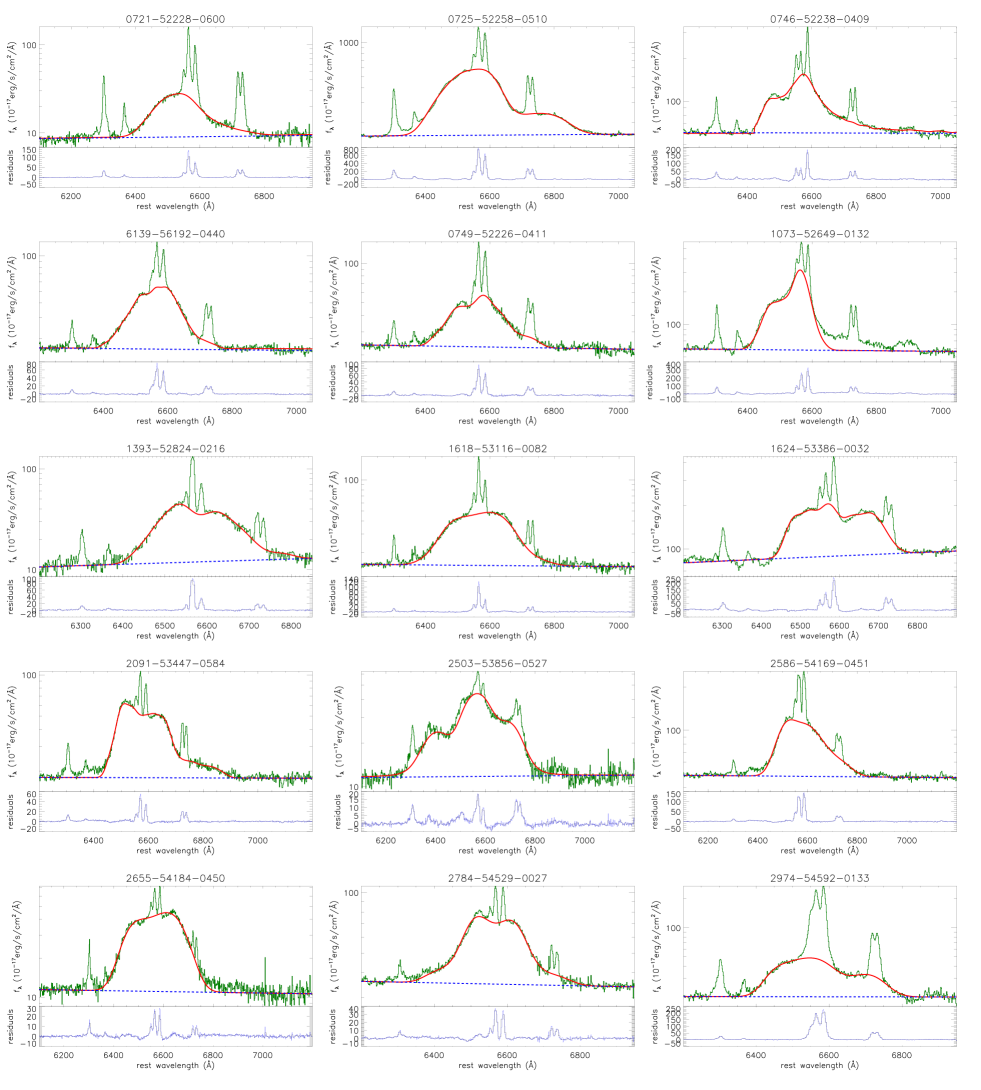
Figure 4: Elliptical accretion disk model determined the best descriptions to the double-peaked broad H$\alpha$. In each panel, solid line in dark green shows the line spectrum after subtractions of the contributions of stellar lights, solid red line shows the elliptical accretion disk model determined best descriptions to the double-peaked broad H$\alpha$, dashed blue line shows the power law continuum emissions similar as the one shown in Figure 2. Bottom region of each panel shows the residuals calculated by line spectrum minus sum of the best descriptions to the double-peaked broad H$\alpha$ plus the power law continuum emissions. In order to show clearly spectral broad emission line features, the Y-axis is in logarithmic coordinate for the plots in top region of each panel.

Figure 4: –continued.

Figure 4: –continued.

Figure 5: SDSS spectrum of NGC5548 (left panel) and the best fitting results to the emission lines around H$\beta$ (middle panel) and around H$\alpha$ (right panel). Symbols and line styles in the middle and the right panel have the same meanings as those in Figure 2.

Figure 6: Top left panel shows an example on the simulating double-peaked broad H$\alpha$ (dark green) and the best-fitting results (red). In left panel, the input and measured values of $r_{0}$, $r_{1}$ and $\sin(i)$ are marked in blue characters. The other panels show the correlations between the six input model parameters and the six re-measured model parameters with corresponding uncertainties determined by the best-fitting results to the simulating double-leaked broad H$\alpha$. In the last six panels, solid red lines and dashed blue lines show the X=Y and the corresponding 99.9999% confidence bands to X=Y.

Figure 7: Properties of $R_{NLRs,u}$ of the 38 double-peaked BLAGN (shown as solid red circles) in the plane of NLRs size versus [O iii] luminosity. Solid circles in dark green are the results for type-2 AGN with measured NLRs sizes discussed in Liu et al. (2013a), solid blue line shows the empirical R-L relation reported in Liu et al. (2013a). Dotted and dashed blue lines show the corresponding 90% and 99.9999% confidence bands of the empirical R-L relation. The three outliers, SDSS 0581-52356-0463, SDSS 1196-52733-0639 and SDSS 2756-54508-0150, are marked as solid purple circles in the figure. Solid cyan circle represents the results for NGC5548. The 500 blue open circles represent the simulating results based on the created $\log(L_{O~{}{\textsc{iii}}})$ line luminosity and the randomly created $\sin(i)$ and redshift.

Table 1: Parameters of the 38 double-peaked BLAGN

PMF	$z$	$f_{[O~{}{\textsc{iii}}]}$	$f_{H\alpha}$	$f_{H\beta}$	$E(B-V)$	$\sin(i)$	$\chi^{2}_{H\beta}$	$\chi^{2}_{H\alpha}$	$\chi^{2}_{disk}$	$f_{5100}$	$R$
0721-52228-0600	0.058	2699$\pm$56	886$\pm$22	307$\pm$37	…	0.325$\pm$0.013	1.14	1.78	1.67	9.34	5811
0725-52258-0510	0.047	25564$\pm$350	8601$\pm$148	2342$\pm$39	0.145	0.318$\pm$0.002	5.16	1.04	0.51	168.83	4766
0746-52238-0409	0.046	2656$\pm$66	442$\pm$25	99$\pm$10	0.31	0.289$\pm$0.001	1.06	0.96	1.65	55.59	5118
6139-56192-0440*	0.096	1946$\pm$73	823$\pm$23	189$\pm$8	0.287	0.555$\pm$0.028	1.18	0.93	1.02	17.85	3868
0749-52226-0411	0.096	2310$\pm$54	909$\pm$37	228$\pm$9	0.216	0.417$\pm$0.012	2.23	1.43	0.22	25.67	7685
1073-52649-0132	0.026	10887$\pm$226	2262$\pm$127	745$\pm$39	…	0.387$\pm$0.021	1.34	0.49	0.06	70.154	2134
1393-52824-0216	0.041	1415$\pm$60	1024$\pm$26	285$\pm$71	0.126	0.394$\pm$0.035	1.08	0.92	0.11	8.561	3342
1618-53116-0082	0.073	2778$\pm$56	675$\pm$20	251$\pm$9	…	0.471$\pm$0.055	1.37	0.65	0.88	18.627	5093
1624-53386-0032	0.0075	2265$\pm$133	1126$\pm$78	206$\pm$21	0.488	0.332$\pm$0.009	0.97	1.09	1.10	56.58	707
2091-53447-0584	0.073	770$\pm$69	480$\pm$18	151$\pm$28	0.02	0.312$\pm$0.002	1.01	0.81	1.42	20.31	7688
2503-53856-0527	0.071	465$\pm$71	235$\pm$16	64$\pm$8	0.147	0.663$\pm$0.059	0.96	0.76	1.03	12.88	3514
2586-54169-0451	0.084	2175$\pm$131	1955$\pm$90	406$\pm$23	0.378	0.254$\pm$0.005	0.73	0.83	1.39	54.78	10950
2655-54184-0450	0.084	596$\pm$63	227$\pm$18	49$\pm$8	0.342	0.412$\pm$2.671∗∗	0.86	0.79	1.25	12.55	6751
2784-54529-0027	0.083	916$\pm$9	355$\pm$15	91$\pm$8	0.202	0.805$\pm$0.125	1.23	1.22	1.82	44.47	3411
2974-54592-0133	0.043	7513$\pm$216	1562$\pm$214	687$\pm$25	…	0.294$\pm$0.022	2.25	0.61	0.58	22.77	4704
0492-51955-0273	0.039	162$\pm$178	80$\pm$9	41$\pm$9	…	0.188$\pm$1.185∗∗	0.82	0.86	1.01	4.14	6653
0581-52356-0463	0.091	217$\pm$24	88$\pm$11	18$\pm$5	0.391	0.165$\pm$0.291∗∗	0.97	0.85	1.19	16.73	18350
0667-52163-0506	0.042	1952$\pm$53	957$\pm$33	302$\pm$18	0.018	0.235$\pm$1.754∗∗	0.82	0.91	1.12	38.56	5744
0784-52327-0594	0.098	331$\pm$16	269$\pm$7	60$\pm$8	0.318	0.575$\pm$0.041	0.97	0.92	1.03	13.28	5697
0827-52312-0023	0.092	6151$\pm$92	1383$\pm$28	396$\pm$16	0.1	0.371$\pm$0.017	1.75	0.91	1.86	140.58	8256
0966-52642-0499	0.096	946$\pm$39	1099$\pm$21	230$\pm$10	0.372	0.806$\pm$0.183	0.98	0.68	0.73	57.88	3431
0972-52435-0520	0.094	2313$\pm$39	685$\pm$31	210$\pm$11	0.043	0.376$\pm$0.011	2.11	0.84	1.15	20.64	8334
1061-52641-0116	0.041	1141$\pm$52	553$\pm$39	80$\pm$15	0.69	0.471$\pm$0.023	1.28	0.63	0.82	95.66	2796
1196-52733-0639	0.022	1289$\pm$66	576$\pm$41	172$\pm$36	0.063	0.089$\pm$0.335∗∗	0.72	0.46	0.68	26.21	7828
1229-52723-0299	0.034	323$\pm$38	324$\pm$18	68$\pm$10	0.37	0.329$\pm$0.018	0.89	0.67	0.73	18.49	3302
1360-53033-0206	0.067	1877$\pm$67	700$\pm$36	192$\pm$19	0.138	0.461$\pm$0.044	1.61	0.64	0.59	36.75	4755
1618-53116-0280	0.074	388$\pm$19	150$\pm$7	39$\pm$5	0.183	0.667$\pm$0.215	0.86	0.92	0.89	9.29	3648
2022-53827-0286	0.023	571$\pm$126	240$\pm$35	63$\pm$15	0.18	0.287$\pm$0.012	0.59	0.35	0.33	20.58	2540
2108-53473-0120	0.023	6708$\pm$162	2310$\pm$162	800$\pm$72	…	0.473$\pm$0.014	1.59	0.41	0.62	249.40	1541
2123-53793-0443	0.077	3786$\pm$227	3531$\pm$252	360$\pm$92	0.994	0.577$\pm$0.095	0.71	0.58	1.02	249.45	4397
2165-53917-0009	0.085	391$\pm$37	170$\pm$23	35$\pm$11	0.384	0.478$\pm$0.024	0.94	0.83	0.97	10.37	5892
2419-54139-0083	0.047	4297$\pm$118	1677$\pm$115	380$\pm$62	0.302	0.655$\pm$0.104	1.52	0.41	0.51	25.21	2314
2477-54058-0014	0.047	587$\pm$191	408$\pm$39	67$\pm$12	0.582	0.522$\pm$0.037	0.81	0.62	0.64	25.24	2904
2593-54175-0208	0.099	440$\pm$27	477$\pm$12	114$\pm$7	0.258	0.416$\pm$0.018	0.82	0.64	0.64	15.28	7960
2756-54508-0150	0.082	637$\pm$19	162$\pm$7	53$\pm$8	…	0.252$\pm$0.009	0.93	0.86	0.96	6.22	10759
2760-54506-0022	0.078	1429$\pm$26	439$\pm$10	125$\pm$7	0.108	0.857$\pm$0.767	1.43	0.90	0.86	10.21	3001
2768-54265-0402	0.091	727$\pm$29	278$\pm$9	78$\pm$7	0.118	0.463$\pm$0.024	0.93	0.91	0.97	27.75	6539
2783-54524-0517	0.055	2197$\pm$82	1932$\pm$47	368$\pm$24	0.455	0.591$\pm$0.034	1.87	0.62	0.58	192.70	3019

Notice: The first and second column show the information of PLATE-MJD-FIBERID and redshift, the third to fifth columns show the line fluxes of [O iii]$\lambda 5007$Å, narrow H$\alpha$ and narrow H$\beta$, in units of $10^{-17}{\rm erg/s/cm^{2}}$, the sixth column shows the corresponding E(B-V) calculated from the flux ratio of narrow H$\alpha$ to narrow H$\beta$, the seventh column shows elliptical accretion disk model determined $\sin(i)$, the eighth, ninth and tenth column show the values of $\chi^{2}$ for the best descriptions to the emission lines around H$\beta$ and around H$\alpha$ by multiple Gaussian functions, and to the broad double-peaked H$\alpha$ by the elliptical accretion disk model, the eleventh column shows the continuum intensity at 5100Å  in the units of $10^{-17}{\rm erg/s/cm^{2}/\textsc{\AA}}$, and the final column shows the estimated upper limit of NLRs sizes $R_{NLRs,u}$ in the units of $pc$.
The first four rows are for the double-peaked BLAGN from the sample of Strateva et al. (2003). The fifth row to the fifteenth row are for the double-peaked BLAGN collected from SDSS quasars. The other rows are for the double-peaked BLAGN collected from the sample of Liu et al. (2019)
SDSS 6139-56192-0440 has its SDSS spectrum from the eBOSS with fiber diameter of 2 arcseconds, and the value $R_{NLRs,u}$ of SDSS 6139-56192-0440 is estimated by the fiber radius of 1 arcseconds.
^∗∗ means that the value is the one determined by the Levenberg-Marquardt least-squares minimization method, although the uncertainty is larger than the value.

Table 2: Parameters of the disk-like BLRs of the 38 double-peaked BLAGN

PMF	$r_{0}$	$r_{1}$	$\sin(i)$	$q$	$\sigma_{L}$	$e$	$\phi_{0}$
	$R_{G}$	$R_{G}$			$km/s$
0721-52228-0600	94$\pm$12	3450$\pm$560	0.325$\pm$0.013	1.98$\pm$0.07	1170$\pm$110	0.20$\pm$0.02	0.32$\pm$0.03
0725-52258-0510	61$\pm$2	1330$\pm$640	0.318$\pm$0.002	4.11$\pm$0.15	1740$\pm$40	0.31$\pm$0.01	1.81$\pm$0.03
0746-52238-0409	29$\pm$1	4826$\pm$420	0.289$\pm$0.001	2.23$\pm$0.01	650$\pm$35	0.78$\pm$0.01	2.47$\pm$0.02
6139-56192-0440	476$\pm$55	5175$\pm$670	0.555$\pm$0.028	2.03$\pm$0.04	460$\pm$50	0.70$\pm$0.01	2.91$\pm$0.01
0749-52226-0411	153$\pm$14	53329$\pm$25296	0.417$\pm$0.012	3.87$\pm$0.07	875$\pm$60	0.58$\pm$0.12	0.24$\pm$0.03
1073-52649-0132	235$\pm$77	3773$\pm$14627	0.387$\pm$0.021	3.05$\pm$0.44	770$\pm$146	0.67$\pm$0.22	0.58$\pm$0.04
1393-52824-0216	159$\pm$27	1911$\pm$1354	0.394$\pm$0.035	3.61$\pm$1.38	1140$\pm$180	0.26$\pm$0.06	0.01$\pm$0.02
1618-53116-0082	175$\pm$46	3485$\pm$2526	0.471$\pm$0.055	3.05$\pm$0.39	1520$\pm$260	0.24$\pm$0.06	0.42$\pm$0.11
1624-53386-0032	148$\pm$8	4633$\pm$678	0.332$\pm$0.009	4.46$\pm$0.16	900$\pm$20	0.57$\pm$0.03	0.01$\pm$0.01
2091-53447-0584	94$\pm$2	2749$\pm$110	0.312$\pm$0.002	2.78$\pm$0.04	770$\pm$30	0.01$\pm$0.01	0.23$\pm$0.02
2503-53856-0527	51$\pm$17	15063$\pm$3562	0.663$\pm$0.059	3.47$\pm$0.21	1610$\pm$45	0.27$\pm$0.03	2.04$\pm$0.04
2586-54169-0451	64$\pm$36	9879∗∗	0.254$\pm$0.005	4.76$\pm$4.96	1620$\pm$460	0.42$\pm$0.24	0.74$\pm$0.98
2655-54184-0450	267∗∗	2343∗∗	0.412$\pm$2.671∗∗	4.07∗∗	1980∗∗	0.28∗∗	0.49∗∗
2784-54529-0027	888$\pm$316	14900∗∗	0.805$\pm$0.125	3.41$\pm$1.08	1300$\pm$310	0.73$\pm$0.61	3.13$\pm$0.02
2974-54592-0133	76$\pm$66	4101∗∗	0.294$\pm$0.022	4.32$\pm$0.42	1530$\pm$115	0.36$\pm$0.36	1.39$\pm$0.38
0492-51955-0273	383∗∗	540∗∗	0.188∗∗	4.47∗∗	1395$\pm$450	0.26∗∗	2.48∗∗
0581-52356-0463	154$\pm$104	729∗∗	0.165∗∗	4.24∗∗	1515$\pm$40	0.56∗∗	2.01∗∗
0667-52163-0506	177∗∗	317∗∗	0.235∗∗	3.85∗∗	1410$\pm$372	0.29∗∗	1.63∗∗
0784-52327-0594	78$\pm$27	4548$\pm$622	0.575$\pm$0.041	1.13$\pm$0.08	934$\pm$62	0.19$\pm$0.01	0.21$\pm$0.01
0827-52312-0023	91$\pm$100	310$\pm$277	0.371$\pm$0.017	2.32∗∗	2451$\pm$92	0.95$\pm$0.01	1.68$\pm$0.08
0966-52642-0499	581$\pm$287	22827$\pm$10699	0.806$\pm$0.183	1.59$\pm$0.07	1174$\pm$44	0.001∗∗	2.41$\pm$0.11
0972-52435-0520	87$\pm$9	5396$\pm$426	0.376$\pm$0.011	1.33$\pm$0.02	1166$\pm$30	0.04$\pm$0.01	1.98$\pm$0.07
1061-52641-0116	164$\pm$23	9663$\pm$1110	0.471$\pm$0.023	1.45$\pm$0.02	930$\pm$34	0.18$\pm$0.02	2.32$\pm$0.06
1196-52733-0639	77$\pm$202	10914∗∗	0.089∗∗	1.83$\pm$2.10	1367$\pm$193	0.00∗∗	2.09∗∗
1229-52723-0299	749$\pm$759	3390$\pm$4338	0.329$\pm$0.018	2.13∗∗	1450$\pm$94	0.00∗∗	2.36∗∗
1360-53033-0206	54$\pm$11	8729$\pm$2078	0.461$\pm$0.044	1.16$\pm$0.05	986$\pm$44	0.03$\pm$0.02	2.18$\pm$0.04
1618-53116-0280	172$\pm$115	23035$\pm$15353	0.667$\pm$0.215	1.28$\pm$0.07	895$\pm$94	0.00∗∗	2.38$\pm$0.24
2022-53827-0286	196$\pm$31	4949$\pm$1532	0.287$\pm$0.012	2.70$\pm$0.08	817$\pm$49	0.57$\pm$0.08	2.16$\pm$0.04
2108-53473-0120	241$\pm$19	5795$\pm$374	0.473$\pm$0.014	1.46$\pm$0.03	800$\pm$25	0.09$\pm$0.01	2.25$\pm$0.01
2123-53793-0443	103$\pm$37	4094$\pm$1532	0.577$\pm$0.096	2.16$\pm$0.35	2290$\pm$77	0.44$\pm$0.14	1.55$\pm$0.09
2165-53917-0009	150$\pm$28	4359$\pm$524	0.478$\pm$0.024	1.36$\pm$0.05	1030$\pm$57	0.06$\pm$0.01	2.42$\pm$0.04
2419-54139-0083	746$\pm$224	11193$\pm$3537	0.655$\pm$0.104	5.77$\pm$2.61	880$\pm$15	0.79$\pm$0.01	3.77$\pm$0.02
2477-54058-0014	181$\pm$36	6080$\pm$946	0.522$\pm$0.037	1.24$\pm$0.04	1175$\pm$48	0.11$\pm$0.01	2.33$\pm$0.06
2593-54175-0208	122$\pm$21	2484$\pm$297	0.416$\pm$0.018	1.29$\pm$0.07	747$\pm$52	0.50$\pm$0.01	2.19$\pm$0.02
2756-54508-0150	168$\pm$20	40329$\pm$31137	0.252$\pm$0.009	2.55$\pm$0.04	678$\pm$72	0.16$\pm$0.05	2.18$\pm$0.04
2760-54506-0022	159∗∗	21907∗∗	0.857$\pm$0.767	0.84$\pm$0.11	1010$\pm$53	0.02$\pm$0.02	1.57$\pm$2.16
2768-54265-0402	201$\pm$29	6911$\pm$930	0.463$\pm$0.024	1.59$\pm$0.04	772$\pm$35	0.14$\pm$0.01	2.23$\pm$0.01
2783-54524-0517	114$\pm$14	21989$\pm$2727	0.591$\pm$0.034	1.46$\pm$0.02	800$\pm$39	0.00∗∗	2.51$\pm$0.01

Notice: ^∗∗ means the model determined value quite smaller than the corresponding uncertainties.
The first four rows are the results for the four double-peaked BLAGN from the sample of Strateva et al. (2003). The fifth row to the fifteenth row are for the double-peaked BLAGN collected from SDSS quasars. The other rows are for the double-peaked BLAGN collected from the sample of Liu et al. (2019)
The listed $\sin(i)$ in the fourth column are the same as the ones listed in the seventh column of Table 1.

Table 3: Line fluxes of broad Balmer emission lines of the 38 double-peaked BLAGN

PMF	$f_{\beta}$	$f_{\alpha}$	rat	$E(B-V)$
0721-52228-0600	588	3246	5.52	0.500
0725-52258-0510	19064	96874	5.08	0.428
0746-52238-0409	3086	14595	4.72	0.365
6139-56192-0440	1167	6299	5.39	0.480
0749-52226-0411	1025	4908	4.78	0.375
1073-52649-0132	6527	15850	2.42	0.000
1393-52824-0216	811	6096	7.51	0.765
1618-53116-0082	1887	8411	4.45	0.312
1624-53386-0032	4234	23628	5.57	0.506
2091-53447-0584	1651	8837	5.34	0.470
2503-53856-0527	1453	7974	5.48	0.487
2586-54169-0451	3238	14724	4.54	0.330
2655-54184-0450	1723	8707	5.05	0.420
2784-54529-0027	2556	8205	3.21	0.027
2974-54592-0133	1498	6813	4.54	0.330
0492-51955-0273	327	1813	5.53	0.498
0581-52356-0463	1065	3714	3.48	0.100
0667-52163-0506	1203	6212	5.16	0.440
0784-52327-0594	575	2363	4.11	0.240
0827-52312-0023	12902	40474	3.13	0.010
0966-52642-0499	2055	7941	3.86	0.185
0972-52435-0520	2067	12542	6.06	0.576
1061-52641-0116	4079	16065	3.93	0.205
1196-52733-0639	1842	8686	4.71	0.360
1229-52723-0299	730	3565	4.88	0.395
1360-53033-0206	1827	8003	4.37	0.301
1618-53116-0280	532	1984	3.72	0.156
2022-53827-0286	2264	11870	5.24	0.449
2108-53473-0120	9630	45910	4.76	0.374
2123-53793-0443	19853	78485	3.95	0.210
2165-53917-0009	741	4097	5.52	0.495
2419-54139-0083	2581	24967	9.67	0.985
2477-54058-0014	2276	9908	4.35	0.295
2593-54175-0208	950	4607	4.84	0.385
2756-54508-0150	417	2238	5.36	0.470
2760-54506-0022	496	2269	4.57	0.331
2768-54265-0402	791	4022	5.08	0.425
2783-54524-0517	3379	14498	4.29	0.275

Notice: The first column shows the information of PLATE-MJD-FIBERID, the second and the third column show the measured line flux of broad H$\beta$ and broad H$\alpha$ in the units of $10^{-17}{\rm erg/s/cm^{2}}$, the fourth column shows the flux ratio of broad H$\alpha$ to broad H$\beta$, the last column shows the calculated $E(B-V)$.
The first four rows are the results for the four double-peaked BLAGN from the sample of Strateva et al. (2003). The fifth row to the fifteenth row are for the double-peaked BLAGN collected from SDSS quasars. The other rows are for the double-peaked BLAGN collected from the sample of Liu et al. (2019).

Then, Figure 7 shows the dependence of $R_{NLRs,u}$ on the [O iii] line luminosity of the 38 low redshift double-peaked BLAGN. Here, based on the intrinsic flux ratio of narrow H$\alpha$ to narrow H$\beta$ as 3.1, reddening effects have been corrected to calculate the intrinsic [O iii] line luminosity for the objects with flux ratios of narrow H$\alpha$ to narrow H$\beta$ larger than 3.1, based on the well applied Galactic extinction curve in Fitzpatrick (1999). The applied values of $E(B-V)$ are also listed in Table 1. More interestingly, the upper limits of NLRs sizes $R_{NLRs,u}$ of the 38 double-peaked BLAGN are not apparently against the expected results from the empirical relation of type-2 AGN in the literature. Based on the linear regression result on the correlation between NLRs sizes and [O iii] luminosities of the type-2 AGN, the 90% and 99.9999% confidence bands are shown for the linear regression result. All the type-2 AGN with measured NLRs sizes shown in Liu et al. (2013a) are lying within the 99.9999% confidence bands. Whereas, there are 35 double-peaked BLAGN lying within the 99.9999% confidence bands, besides the three objects SDSS 0581-52356-0463, SDSS 1196-52733-0639 and SDSS 2756-54508-0150 above the upper boundary of the 99.9999% confidence bands. The three objects are shown in Figure 7 as solid purple circles.

However, considering the quite large uncertainties of NLRs sizes and the NLRs sizes as upper limits, it is hard to conclude that SDSS 0581-52356-0463, SDSS 1196-52733-0639 and SDSS 2756-54508-0150 do not obey the dependence of NLRs sizes on [O iii] luminosity from type-1 AGN. In the near future, large sample of low redshift double-peaked BLAGN in SDSS could provide further clues on whether are there different dependence of NLRs size on [O iii] luminosity between type-1 AGN and type-2 AGN. In the current stage, the simple conclusion can be well reached that there are the similar dependence of NLRs sizes on [O iii] luminosity between the type-1 AGN and the type-2 AGN, indicating no apparent clues to against the expected results from the unified model for different kinds of AGN.

Before further discussions on the results shown in Figure 7, it is necessary to consider whether the SDSS fibers cover all the [O iii] emissions of the 38 low redshift double-peaked BLAGN? We answer the question as follows. As what we have known that there is one strong linear correlation between continuum luminosity and [O iii] luminosity of QSOs, see our previous results in Zhang et al. (2017b) and results in Shen et al. (2011) and results in rakshit et al. (2020), if the SDSS fibers only cover part of [O iii] emissions, the observed [O iii] luminosity could be smaller than the expected value from the continuum luminosity, because the continuum emissions of type-1 AGN are totally covered by the SDSS fibers. Therefore, we check the correlation between continuum luminosity and [O iii] luminosity of the 38 double-peaked BLAGN. Here, based on the intrinsic flux ratio of broad H$\alpha$ to broad H$\beta$ as 3.1, intrinsic reddening effects have been corrected to calculate the intrinsic continuum luminosity for the objects with flux ratios of broad H$\alpha$ to broad H$\beta$ larger than 3.1, based on the well applied Galactic extinction curve in Fitzpatrick (1999). The line fluxes of the broad Balmer lines are calculated by sum of the fluxes of the broad Gaussian components shown as solid lines in Figure 2 and listed in Table 3. The applied $E(B-V)$ to correct continuum emissions are also listed in Table 3. The correlations are shown in left panel of Figure 8 between the reddening corrected continuum luminosity and [O iii]  line luminosity for the type-1 AGN discussed in Zhang et al. (2017b) and for the quasars in Shen et al. (2011) and for the quasars in rakshit et al. (2020). Based on the shown results in left panel of Figure 8, two points can be found. On the one hand, the results in Zhang et al. (2017b) are well consistent with those in Shen et al. (2011) and in rakshit et al. (2020), to support the robust correlation between continuum luminosity and [O iii]  line luminosity in type-1 AGN. On the other hand, the observed [O iii] luminosities are not statistically smaller than the expected values through the continuum luminosities. Based on the results shown in the left panel of Figure 8, the mean values of continuum luminosity to [O iii]  line luminosity $\log(L_{5100})-\log(L_{[O~{}\textsc{iii}]})$ are about 2.49$\pm$0.31, 2.49$\pm$0.37, 2.57$\pm$0.41 and 2.51$\pm$0.36 for the type-1 AGN in Zhang et al. (2017b), for the quasars in Shen et al. (2011), for the quasars in rakshit et al. (2020), and for the 38 double-peaked BLAGN, respectively, with the standard deviations as the uncertainties of the mean values. Student’s T-statistic technique is applied to confirm significance level higher than 75% that the normal type-1 AGN and the 38 double-peaked BLAGN have the same mean values of $\log(L_{5100})-\log(L_{[O~{}\textsc{iii}]})$. Therefore, the calculated $R_{NLRs,u}$ are truly the upper limits of sizes of NLRs of the 38 double-peaked BLAGN, after accepted that the [O iii] emission regions are expected to be totally covered in SDSS fibers.

Before given the final conclusions, it is necessary to check whether randomly collected values of $\sin(i)$ can lead to similar results as those in Figure 7 for the final sample of the 38 low redshift double-peaked BLAGN. A simple procedure is applied as follows. There are 500 values of $\sin(i)$ randomly created with inclination angle $i$ from 20°  to 70°, 500 values of redshift randomly created from 0 and 0.1. For the [O iii] line luminosity $\log(L_{[O~{}\textsc{iii}]})$, the values are created as follows. Based on the reported $\log(L_{[O~{}\textsc{iii}]})$ in Zhang et al. (2017b) of the 149 low-redshift Type-1 AGN with $z<0.1$, distribution of $\log(L_{[O~{}\textsc{iii}]})$ of the 149 quasars shown in right panel of Figure 8 has a Gaussian profile with mean value of 41.3 and standard deviation of 0.48. Although Shen et al. (2011) and rakshit et al. (2020) have reported large samples of SDSS quasars, there are only 21 quasars with redshift smaller than 0.1 in the sample of Shen et al. (2011), and only 53 quasars with redshift smaller than 0.1 in the sample of rakshit et al. (2020). Therefore, there are no further considerations of the low redshift quasars in Shen et al. (2011); rakshit et al. (2020) in right panel of Figure 8. Based on the Gaussian distribution of $\log(L_{[O~{}\textsc{iii}]})$ for quasars with $z<0.1$, 500 values of $\log(L_{[O~{}\textsc{iii}]})$ are created. Then, based on the 500 created $\log(L_{[O~{}\textsc{iii}]})$ and the 500 randomly created redshift and $\sin(i)$, the simulating dependence of upper limits of NLRs sizes on [O iii] line luminosity is shown as blue open circle in Figure 7. It is clear that there are more than one third of the 500 simulating data points lying out of the 99.9999% confidence interval of the expected results from the empirical relation between NLRs sizes and [O iii]  luminosity in the type-2 AGN. However, among the 38 low-redshift double-peaked BLAGN in our final sample, only three objects lying out of the 99.9999% confidence interval. Therefore, the results of the 38 double-peaked BLAGN in Figure 7 have real physical properties.

Moreover, as we have discussed in Section 2, the long-term variabilities of the 38 double-peaked BLAGN should be checked, in order to ignore the probable BBHs model applied to describe the double-peaked broad H$\alpha$. The long-term light curves have been collected from the CSS and shown in Figure 9 for the 37 double-peaked BLAGN, besides the SDSS 2123-53793-0443 without light curve provided by the CSS. The commonly accepted generalized Lomb-Scargle technique (GLS) (Lomb, 1976; Scargle, 1982; Zechmeister & Kurster, 2009; Zheng et al., 2016) is applied to check the probable QPOs signs. Here, as shown in Figure 9, there are no signs for apparent QPOs in the 37 double-peaked BLAGN. So that, there are no further discussions on the results in Figure 9, and the BBH model is not preferred in the collected double-peaked BLAGN. The results shown in Figure 7 are the basic and natural results on the upper limits of NLRs sizes after considerations of inclinations.

Figure 8: Left panel shows the correlation between continuum luminosity and [O iii]  luminosity. Solid dots plus error bars are the results for the type-1 AGN discussed in Zhang et al. (2017b). Contour in bluish colors represents the results for the quasars collected from Shen et al. (2011), with the color bar in bluish colors shown in top corner of the left panel. Contour in reddish colors represents the results for the quasars collected from rakshit et al. (2020), with the color bar in bluish colors shown in top corner of the left panel. Solid red circles plus error bars are the results for the 38 low redshift double-peaked BLAGN in the final sample after intrinsic reddening corrections. Solid dark green line and solid red lines show the best-fitting results and corresponding 2.6RMS scatters to the correlation. Right panel shows the distributions of $\log(L_{[O~{}\textsc{iii}]})$ of the 149 Type-1 AGN with redshift smaller than 0.1 in the sample of Zhang et al. (2017b).

Figure 9: Light curves of the 37 double-peaked BLAGN (panels in the first and the third column) and the corresponding GLS properties applied to detect QPOs signs ( panels in the second and the fourth column). In each panel for the GLS power properties, horizontal dashed red line shows the 99.99% confidence level (0.0001 as the false-alarm probability) for the probable periodicity.

Figure 9: –continued.

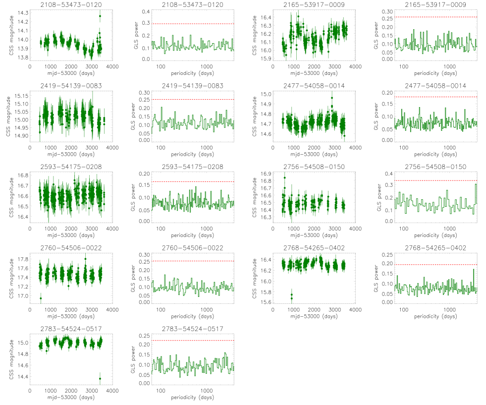
Figure 9: –continued.

5 Summaries and Conclusions

Finally, we give our main summaries and conclusions as follows.

• Double-peaked broad H$\alpha$ of 38 low redshift ($z<0.1$) double-peaked BLAGN can be well described by the elliptical accretion disk model, accepted the accretion disk origin of double-peaked broad emission lines leading to the well determined inclinations of central line emission regions.

• Considering the fixed SDSS fibers and the determined inclinations, upper limits of NLRs sizes in the 38 double-peaked BLAGN can be well estimated.

• The strong linear correlation between continuum luminosity and [O iii] luminosity can be well applied to confirm that the [O iii] emissions of the 38 low redshift double-peaked BLAGN are totally covered in the SDSS fibers, indicating the estimated upper limits of NLRs sizes are reliable.

• There are no QPOs signs in the long-term light curves of the collected low redshift double-peaked BLAGN, indicating the proposed BBH model is not preferred to explain the double-peaked broad H$\alpha$ of the low redshift double-peaked BLAGN.

• The 38 double-peaked BLAGN have their upper limits of NLRs sizes not statistically against the expected results through the R-L relation for NLRs in type-2 AGN, indicating that the current results can not provide clues to challenge the Unified model through the space properties of NLRs.

Data Availability

The data and program underlying this article will be shared on reasonable request to the corresponding author (xgzhang@njnu.edu.cn).

References

- Ahumada et al. (2020) Ahumada, Romina; Prieto, Carlos Allende; Almeida, A, et al., 2020, ApJS, 249, 3
- Antouncci (1993) Antonucci, R., 1993, ARA&A, 31, 473
- Antonucci & Miller (1985) Antonucci, R. J.; Miller, J. S. 1985, ApJ, 297, 621
- Barth et al. (2014) Barth, A. J.; Voevodkin, A.; Carson, D. J.; Wozniak, P., 2014, ApJ, 147, 12
- Barth et al. (2015) Barth, A. J.; Bennert, V. N.; Canalizo, G., et al., 2015, ApJS, 217, 26
- Begelman et al. (1980) Begelman, M. C.; Blandford, R. D.; Rees, M. J., 1980, Natur, 287, 307
- Bennert et al. (2002) Bennert, N.; Falcke, H., Schulz, H., et al., 2002, ApJL, 574, L105
- Bennert et al. (2006a) Bennert, N.; Jungwiert, B.; Komossa, S.; Haas, M.; Chini, R., 2006a, A&A, 446, 919
- Bennert et al. (2006b) Bennert, N.; Jungwiert, B.; Komossa, S.; Haas, M.; Chini, R., 2006b, A&A, 456, 953
- Bentz et al. (2010) Bentz, Misty C.; Walsh, Jonelle L.; Barth, A. J., et al., 2010, ApJ, 716, 993
- Bentz et al. (2013) Bentz, M. C.; Denney, K. D.; Grier, C. J.; et al., 2013, ApJ, 767, 149
- Bianchi et al. (2019) Bianchi, S.; Antonucci, R.; Capetti, A; et al., 2019, MNRAS Letter, 488, 1
- Blandford & McKee (1982) Blandford, R. D.; McKee, C. F., 1982, ApJ, 255, 419
- Bruzual & Charlot (2003) Bruzual, G., & Charlot, S. 2003, MNRAS, 344, 1000
- Cardamone et al. (2007) Cardamone, C. N.; Moran, E. C.; Kay, L. E., 2007, AJ, 134, 1263
- Chen & Halpern (1989) Chen, K. Y., & Halpern, J. P., 1989, ApJ, 344, 115
- Cid Fernandes et al. (2005) Cid Fernandes, R., Mateus, A., Sodre, L., Stasinska, G., Gomes, J. M., 2005, MNRAS, 358, 363
- Dempsey & Zakamska (2018) Dempsey, R.; Zakamska, N. L., 2018, MNRAS, 477, 4615
- Di Matteo et al. (2005) Di Matteo, T., Springel, V., Hernquist, L. 2005, Natur, 433, 604
- Drake et al. (2009) Drake, A. J.; Djorgovski, S. G.; Mahabal, A.; et al., 2009, ApJ, 696, 870
- Du et al. (2016) Du, P., Lu, K., Zhang Z., et al., 2016, ApJ, 825, 126
- Eracleous et al. (1995) Eracleous, M., Livio, M., Halpern, J. P., Storchi-Bergmann, T.,1995, ApJ, 438, 610
- Eracleous et al. (1997) Eracleous, M., Halpern, J. P., Gilbert, A. M., Newman, J. A., Filippenko, A. V., 1997, ApJ, 490, 216
- Fischer et al. (2018) Fischer, T., Kraemer, S., Schmitt, H., et al., 2018, ApJ, 856, 102
- Fitzpatrick (1999) Fitzpatrick, E. L., 1999, PASP, 111, 63
- Flohic & Eracleous (2008) Flohic, H. M. L. G., & Eracleous, M., 2008, ApJ, 686, 138
- Gaskell (1996) Gaskell, M., 1996, ApJ, 464, 107
- Greene et al. (2011) Greene, J. E.; Zakamska, N. L.; Ho, L. C.; Barth, A. J., 2011, ApJ, 732, 9
- Graham et al. (2015a) Graham, M. J.; Djorgovski, S. G.; Stern, D., et al., 2015a, Natur, 518, 74
- Graham et al. (2015b) Graham, M. J., Djorgovski, S. G., Stern, D., et al., 2015b, MNRAS, 453, 1562
- Grier et al. (2017) Grier, C. J.; Trump, J. R.; Shen, Y., et al., 2017, ApJ, 851, 21
- Greene et al. (2011) Greene, J. E.; Zakamska, N. L.; Ho, L. C.; Barth, A. J., 2010, ApJ, 732, 9
- Hainline et al. (2013) Hainline, K., Hickox, R., Greene, J., et al., 2013, ApJ, 774, 145
- Hainline et al. (2014) Hainline, K., Hickox, R., Greene, J., et al., 2014, ApJ, 787, 65
- Hartnoll & Blackman (2000) Hartnoll, S. A.; Blackman, E. G., 2000, MNRAS, 317, 880
- Kaspi et al. (2000) Kaspi, S.; Smith, P. S.; Netzer, H.; et al., 2000, ApJ, 533, 631
- Kaspi et al. (2005) Kaspi, S.; Maoz, D.; Netzer, H., et al., 2005, ApJ, 629, 61
- Kauffmann et al. (2003) Kauffmann, G., et al. 2003, MNRAS, 346, 1055
- Kovacevic-Dojcinovic et al. (2010) Kovacevic, J.; Popovic, L. C.; Dimitrijevic, M. S., 2010, ApJS, 189, 15
- Lewis, Eracleous & Storchi-Bergmann (2010) Lewis, K. T., Eracleous, M., & Storchi-Bergmann, T., 2010, ApJS, 187, 416
- Liao et al. (2021) Liao, Wei-Ting; Chen, Yu-Ching; Liu, X.; et al., 2021, MNRAS, 500, 4025
- Liu et al. (2013a) Liu G., Zakamska, N., Greene, J., et al., 2013a, MNRAS, 430, 2327
- Liu et al. (2013b) Liu G., Zakamska, N., Greene, J., et al., 2013b, MNRAS, 436, 2576
- Liu et al. (2019) Liu, H.; Liu, W.; Dong, X.; Zhou, H.; Wang, T.; Lu, H.; Yuan, W., 2019, ApJS, 243, 21
- Lomb (1976) Lomb, N. R. 1976, Ap&SS, 39, 447
- Markwardt (2009) Markwardt, C. B., 2009, ASPC, 411, 251
- Nagao et al. (2004) Nagao, T.; Kawabata, K. S.; Murayama, T.; Ohyama, Y.; Taniguchi, Y.; Sumiya, R.; Sasaki, S. S., 2004, ApJ, 128, 109
- Netzer (2015) Netzer, H., 2015, ARA&A, 53, 365
- Peterson et al. (2004) Peterson, B. M.; Ferrarese, L.; Gilbert, K. M.; et al., 2004, ApJ, 613, 682
- Pons & Watson (2016) Pons, E.; Watson, M. G., 2016, A&A, 594, 72
- Pfister et al. (2017) Pfister, Hugo; Lupi, Alessandro; Capelo, Pedro R.; et al., 2017, MNRAS, 371, 3646
- rakshit et al. (2020) Rakshit, S.; Stalin, C. S.; Kotilainen, J., 2020, ApJS, 249, 17
- Sayeb et al. (2021) Sayeb, M.; Blecha, L.; Kelley, L. Z.; et al., 2021, MNRAS, 501, 2531
- Savic et al. (2018) Savic, D.; Goosmann, R.; Popovic, L. C.; Marin, F.; Afanasiev, V. L., 2018, A&A, 614, 120
- Scargle (1982) Scargle, J. D. 1982, ApJ, 263, 835
- Schmitt et al. (2003a) Schmitt, H., Donley, J., Antonucci, R., et al., 2003a, ApJ, 597, 768
- Schmitt et al. (2003b) Schmitt, H., Donley, J., Antonucci, R., et al., 2003b, ApJS, 148, 327
- Shapovalova et al. (2001) Shapovalova, A. I., et al., 2001, A&A, 376, 775
- Shen & Loeb (2010) Shen, Y.; Loeb, A., 2010, ApJ, 725, 249
- Shen et al. (2011) Shen, Y.; Richards, G. T.; Strauss, M. A.; et al., 2011, ApJS, 194, 45
- Shen et al. (2015) Shen, Y., et al., 2015, ApJS, 216, 4
- Shi et al. (2010) Shi, Y.; Rieke, G. H.; Smith, P.; et al., 2010, ApJ, 714, 115
- Storchi-Bergmann et al. (2003) Storchi-Bergmann, T., et al., 2003, ApJ, 489, 8
- Storchi-Bergmann et al. (2017) Storchi-Bergmann, T., et al., 2017, ApJ, 835, 236
- Strateva et al. (2003) Strateva, I. V., et al., 2003, AJ, 126, 1720
- Tran (2001) Tran, H. D., 2001, ApJL, 554, 19
- Tran (2003) Tran, H. D., 2003, ApJ, 583, 632
- Wang et al. (2014) Wang, J.-M., Du, P., Hu, C., et al., 2014, ApJ, 793, 108
- Zhang et al. (2005) Wang, T. G.; Dong, X. B.; Zhang, X. G., et al. 2005, ApJ Letter, 625, 35
- Williams et al. (2018) Williams, P. R.; Pancoast, A.; Treu, T., et al., 2018, ApJ, 866, 75
- Zechmeister & Kurster (2009) Zechmeister, M.; Kurster, M., 2009, A&A, 496, 577
- Zhang (2013a) Zhang, X. G., 2013a, MNRAS, 429, 2274
- Zhang (2013) Zhang, X.-G., 2013, MNRAS Letter, 431, 112
- Zhang (2014) Zhang, X. G., 2014, MNRAS, 438, 557
- Zhang (2015) Zhang, X. G., 2015, MNRAS Letter, 447, 35
- Zhang et al. (2016) Zhang, X. G., Feng, L. L., 2016, MNRAS, 457, 3878
- Zhang & Feng (2017) Zhang, X. G., Feng L., 2017, MNRAS, 464, 2203
- Zhang et al. (2017b) Zhang, X. G. & Feng, L. L., 2017b, MNRAS, 468, 620
- Zhang et al. (2019) Zhang, X. G.,; Bao, M., Yuan, Q. R., 2019, MNRAS Letter, 490, 81
- Zhang et al. (2020) Zhang, X. G.; Feng, Y. Q.; Chen, H.; Yuan, Q., 2020, ApJ, 905, 97
- Zhang (2021a) Zhang, X. G., 2021a, ApJ, 909, 16, ArXiv:2101.02465
- Zhang (2021b) Zhang, X. G., 2021b, ApJ accepted, Arxiv:2107.09214
- Zhang et al. (2021) Zhang, X. G., Zhang, Y. F., Cheng, P., et al., 2021c, ApJ, 922, 248, Arxiv:2109.02189
- Zhang (2022) Zhang, X. G., 2022, MNRAS accepted, Arxiv:2202.11995
- Zheng et al. (2016) Zheng Z., Butler N. R., Shen Y., Jiang L., Wang J., Chen X., Cuadra, J., 2016, ApJ, 827, 56