Robustness Against Weak or Invalid Instruments: Exploring Nonlinear Treatment Models with Machine Learning

Abstract

We discuss causal inference for observational studies with possibly invalid instrumental variables. We propose a novel methodology called two-stage curvature identification (TSCI) by exploring the nonlinear treatment model with machine learning. The first-stage machine learning enables improving the instrumental variable’s strength and adjusting for different forms of violating the instrumental variable assumptions. The success of TSCI requires the instrumental variable’s effect on treatment to differ from its violation form. A novel bias correction step is implemented to remove bias resulting from the potentially high complexity of machine learning. Our proposed TSCI estimator is shown to be asymptotically unbiased and Gaussian even if the machine learning algorithm does not consistently estimate the treatment model. Furthermore, we design a data-dependent method to choose the best among several candidate violation forms. We apply TSCI to study the effect of education on earnings.

Keywords: Generalized IV strength, Confidence interval, Random forests, Boosting, Neural network.

1 Introduction

Observational studies are major sources for inferring causal effects when randomized experiments are not feasible. But such causal inference from observational studies requires strong assumptions and may be invalid due to the presence of unmeasured confounders. The instrumental variable (IV) regression is a practical and highly popular causal inference approach in the presence of unmeasured confounders. The IVs are required to satisfy three assumptions: conditioning on the baseline covariates, (A1) the IVs are associated with the treatment; (A2) the IVs are not associated with the unmeasured confounders; (A3) the IVs do not directly affect the outcome.

Despite the popularity of the IV method, there is a significant concern about whether the used IVs satisfy (A1)-(A3) in practice. Assumption (A1) requires the IV to be strongly associated with the treatment variable, which can be checked with an F-test in a first-stage linear regression model. Inference with the assumption (A1) being violated has been actively investigated under the name of weak IV (Stock et al., 2002; Staiger and Stock, 1997, e.g.). Assumptions (A2) and (A3) ensure that the IV only affects the outcome through the treatment. If an IV violates either (A2) or (A3), we call it an invalid IV and define its functional form of violating (A2) and (A3) as the violation form, e.g., a linear violation. In the just-identification regime, most empirical analyses rely on external knowledge to argue about the validity of (A2) and (A3). However, there is a pressing need to develop a robust causal inference method against the proposed IVs violating the classical assumptions.

1.1 Our results and contribution

We aim to devise a robust IV framework that leads to causal identification even if the IVs proposed by domain experts may violate assumptions (A1) to (A3). Our framework provides a robustness guarantee even when all proposed IVs are invalid, including the most common regime with a single IV that is possibly invalid. It is well known that the treatment effect is not identifiable when there is no constraint on how the IVs violate assumptions (A2) and (A3). Our key identification assumption is that the violations of (A2) and (A3) arise from simpler forms than the association between the treatment and the IVs; that is, we exclude “special coincidences” such as the IVs violate (A2) and (A3) by linear forms and the conditional mean model of the treatment given IVs is also linear. This identification condition can be evaluated with the generalized IV strength measure introduced in Section 3.3 for a user-specific violation form.

We propose a novel two-stage curvature identification (TSCI) method to infer the treatment effect. An important operational step is to fit the treatment model with a machine learning (ML) algorithm, e.g., random forests, boosting, or deep neural networks. This first-stage ML model enhances the IV’s strength by learning a general conditional mean model of treatment given the IVs, instead of restricting to a linear association model. In the second stage, we leverage the ML prediction and adjust for different IV violation forms. A main novelty of our proposal is to estimate the bias resulting from high complexity of the first-stage ML and implement a corresponding bias correction step; see more details in Section 3.2.

We show that the TSCI estimator is asymptotically Gaussian when the generalized IV strength measure is sufficiently large. We further devise a data-dependent way of choosing the most suitable violation form among a collection of IV violation forms. By including the valid IV setting into the selection, our proposed general TSCI methodology does not exclude the possibility of the IVs being valid but provides a robust IV method against different invalidity forms.

To sum up, the contribution of the current paper is two-fold:

1. TSCI explores a nonlinear treatment model with ML and leads to more reliable causal conclusions than existing methods assuming valid IVs.

2. TSCI provides an efficient way of integrating the first-stage ML. A methodological novelty of TSCI is its bias correction in its second stage, which addresses the issue of high complexity and potential overfitting of ML.

1.2 Comparison to existing literature

There is relevant literature on causal inference when assumptions (A2) and (A3) are violated. When all IVs are invalid, Lewbel (2012); Tchetgen et al. (2021) proposed an identification strategy by assuming that the treatment model has heteroscedastic error but the covariance between the treatment and outcome model errors is homoscedastic. Our proposed TSCI is based on a different idea by exploring the nonlinear structure between the treatment and the IVs, not requiring anything on homo- and heteroscedasticity. Bowden et al. (2015) and Kolesár et al. (2015) assumed that the direct effect of the IVs on the outcome is nearly orthogonal to the effect of the IVs on the treatment. Han (2008); Bowden et al. (2016); Kang et al. (2016); Windmeijer et al. (2019); Guo et al. (2018); Windmeijer et al. (2021) considered the setting that a proportion of IVs are valid and conducted causal inference by selecting valid IVs in a data-dependent way. Along this line, Guo (2023) proposed a uniform inference procedure that is robust to the IV selection error. More recently, Sun et al. (2023) leveraged the number of valid IVs and used the interaction of genetic markers to identify the causal effect. In contrast to assuming the orthogonality and existence of valid IVs, our proposed TSCI is effective even if all IVs are invalid and the effect orthogonality condition does not hold. Such a setting is especially useful in handling econometric applications with a single IV.

The nonlinear structure of the treatment model has been explored in the econometric and the more recent ML literature. In the IV literature, Kelejian (1971); Amemiya (1974); Newey (1990); Hausman et al. (2012) considered constructing a non-parametric treatment model and Belloni et al. (2012) proposed constructing the optimal IVs with a Lasso-type first-stage estimator. More recently, Chen et al. (2023); Liu et al. (2020) proposed constructing the IV as the first-stage prediction given by the ML algorithm. All of the above works are focused on the valid IV setting. In contrast, our current paper applies to the more robust regime where the IVs are allowed to violate assumptions (A2) or (A3) in a range of forms. Even in the context of valid IVs, our proposed TSCI may lead to a more accurate estimator than directly using the predicted value for the treatment model as the new IV (Chen et al., 2023; Liu et al., 2020); see Section 3.5 for details.

ML algorithms integrated into the IV analysis to better accommodate the complicated outcome model. In Sections 3.5 and 5.1, we provide detailed comparisons to Double Machine Learning (DML) proposed in Chernozhukov et al. (2018). Athey et al. (2019) proposed the generalized random forests to infer heterogeneous treatment effects. Both works are based on valid IVs, while our current paper assumes a homogeneous treatment effect and focuses on the different robust IV framework with possibly invalid IVs.

Finally, our proposed TSCI methodology can be used to check the IV validity for the just-identification case. This is distinct from the Sargan test, J test, or specification test (Hansen, 1982; Sargan, 1958; Woutersen and Hausman, 2019) which are used to test IV validity in the over-identification case.

Notation. For a matrix $X\in\mathbb{R}^{n\times p}$, a vector $x\in\mathbb{R}^{n}$, and a set $\mathcal{A}\subset\{1,\cdots,n\}$, we use $X_{\mathcal{A}}$ to denote the submatrix of $X$ whose row indices belong to $\mathcal{A}$, and $x_{\mathcal{A}}$ to denote the sub-vector of $x$ with indices in $\mathcal{A}.$ For a set $\mathcal{A}$, $\left|\mathcal{A}\right|$ denotes its cardinality. For a vector $x\in\mathbb{R}^{p}$, the $\ell_{q}$ norm of $x$ is defined as $\|x\|_{q}=\left(\sum_{l=1}^{p}|x_{l}|^{q}\right)^{\frac{1}{q}}$ for $q\geq 0$ with $\|x\|_{0}=\left|\{1\leq l\leq p:x_{l}\neq 0\}\right|$ and $\|x\|_{\infty}=\max_{1\leq l\leq p}|x_{l}|$. We use $c$ and $C$ to denote generic positive constants that may vary from place to place. For a sequence of random variables $X_{n}$ indexed by $n$, we use $X_{n}\overset{p}{\to}X$ and $X_{n}\overset{d}{\to}X$ to represent that $X_{n}$ converges to $X$ in probability and in distribution, respectively. For two positive sequences $a_{n}$ and $b_{n}$, $a_{n}\lesssim b_{n}$ means that $\exists C>0$ such that $a_{n}\leq Cb_{n}$ for all $n$; $a_{n}\asymp b_{n}$ if $a_{n}\lesssim b_{n}$ and $b_{n}\lesssim a_{n}$, and $a_{n}\ll b_{n}$ if $\limsup_{n\rightarrow\infty}{a_{n}}/{b_{n}}=0$. For a matrix $M$, we use ${\rm Tr}[M]$ to denote its trace, ${\rm rank}(M)$ to denote its rank, and $\|M\|_{F}$, $\|M\|_{2}$ and $\|M\|_{\infty}$ to denote its Frobenius norm, spectral norm and element-wise maximum norm, respectively. For a square matrix $M$, $M^{2}$ denotes the matrix multiplication of $M$ by itself. For a symmetric matrix $M$, we use $\lambda_{\max}(M)$ and $\lambda_{\min}(M)$ to denote its maximum and minimum eigenvalues, respectively.

2 Invalid instruments: modeling and identification

We consider i.i.d. data $\{Y_{i},D_{i},Z_{i},X_{i}\}_{1\leq i\leq n},$ where for the $i$-th observation, $Y_{i}\in\mathbb{R}$ and $D_{i}\in\mathbb{R}$ respectively denote the outcome and the treatment and $Z_{i}\in\mathbb{R}^{p_{z}}$ and $X_{i}\in\mathbb{R}^{p_{x}}$ respectively denote the IVs and measured covariates.

2.1 Examples for effect identification with nonlinear treatment models

To explain the main idea, we start with the special case with no covariates,

$$Y_{i}=D_{i}\beta+Z_{i}^{\intercal}\pi+\epsilon_{i},\quad\text{and}\quad D_{i}=f(Z_{i})+\delta_{i},\quad\text{for}\quad 1\leq i\leq n,$$ (1)

where the errors $\epsilon_{i}$ and $\delta_{i}$ satisfy ${\mathbf{E}}(\epsilon_{i}\mid Z_{i})=0$ and ${\mathbf{E}}(\delta_{i}\mid Z_{i})=0.$ These errors $\epsilon_{i}$ and $\delta_{i}$ are typically correlated due to unobserved confounding. The outcome model in (1) is commonly used in the invalid IV literature (Small, 2007; Kang et al., 2016; Guo et al., 2018; Windmeijer et al., 2019), with $\pi\neq 0$ standing for the violation of IV assumptions (A2) and (A3). The treatment model in (1) is not a causal generating model between $D_{i}$ and $Z_{i}$ but only stands for a probability model between $D_{i}$ and $Z_{i}$. Specifically, the treatment assignment might be directly influenced by unmeasured confounders, but the treatment model in (1) does not explicitly state this generating process. Instead, for the joint distribution of $D_{i}$ and $Z_{i}$, we define the conditional expectation $f(Z_{i})={\mathbf{E}}(D_{i}\mid Z_{i}),$ which leads to the treatment model in (1). We discuss the structural equation model interpretation of the model (1) in Section 2.3, which explicitly characterizes how unmeasured confounders may affect the treatment assignment.

We introduce some projection notations to facilitate the discussion. For a random variable $U_{i}$, define its best linear approximation by $Z_{i}$ as $\gamma^{*}=\operatorname*{arg\,min}_{\gamma\in\mathbb{R}^{p_{z}+1}}{\mathbf{E}}(U_{i}-\widetilde{Z}_{i}^{\intercal}\gamma)^{2}$ with $\widetilde{Z}_{i}=(1,Z_{i}^{\intercal})^{\intercal}$. For $1\leq i\leq n$, write $\mathcal{P}_{Z_{i}}U_{i}=\widetilde{Z}_{i}^{\intercal}\gamma^{*}$ and $\mathcal{P}^{\perp}_{Z_{i}}U_{i}=U_{i}-\widetilde{Z}_{i}^{\intercal}\gamma^{*}.$ We apply $\mathcal{P}^{\perp}_{Z_{i}}$ to the model (1) and obtain $\mathcal{P}^{\perp}_{Z_{i}}Y_{i}=\mathcal{P}^{\perp}_{Z_{i}}D_{i}\beta+\mathcal{P}^{\perp}_{Z_{i}}\epsilon_{i}$, where the linear violation form $Z_{i}^{\intercal}\pi$ in (1) is removed after applying the transformation $\mathcal{P}^{\perp}_{Z_{i}}$. If $f$ is nonlinear, then ${\rm Var}\left(\mathcal{P}^{\perp}_{Z_{i}}f(Z_{i})\right)>0$ and the adjusted variable $\mathcal{P}^{\perp}_{Z_{i}}f(Z_{i})$ can be used as a valid IV to identify the effect $\beta$ via the following estimating equation

$${\mathbf{E}}\left[\mathcal{P}^{\perp}_{Z_{i}}f(Z_{i})(Y_{i}-D_{i}\beta)\right]={\mathbf{E}}\left[\mathcal{P}^{\perp}_{Z_{i}}f(Z_{i})(Z_{i}^{\intercal}\pi+\epsilon_{i})\right]=0.$$ (2)

Note that the last equality follows from the population orthogonality between $\mathcal{P}^{\perp}_{Z_{i}}f(Z_{i})$ and $Z_{i}$, together with ${\mathbf{E}}(\epsilon_{i}\mid Z_{i})=0.$

The estimation equation in (2) reveals that the treatment effect $\beta$ can be identified by exploring the nonlinear structure of $f$ under the model (1). We propose to learn $f$ using a ML prediction model and measure the variability of $\mathcal{P}^{\perp}_{Z_{i}}f(Z_{i})$ by defining a notation of generalized IV strength in Section 3.3. We shall emphasize that using ML algorithms to learn the possibly nonlinear function $f$ is critical in the current framework, allowing for invalid IVs. The ML algorithms help capture complicated structures in $f$ and typically retain enough variability contained in the adjusted variable $\mathcal{P}^{\perp}_{Z_{i}}f(Z_{i})$. In Section A.1 in the supplement, we present another example for causal identification in the context of the randomized experiments with non-compliance and invalid IVs.

Remark 1

Nonlinear functional form identification has been proposed in various existing literature; see Lewbel (2019)[Sec.3.7] for a review. More concretely, Angrist and Pischke (2009)[Sec.4.6.1] discussed the identification of when the IV has a linear direct effect on the outcome, but the treatment model is a nonlinear parametric model of the IV. The Heckman selection model Heckman (1976) offered a practical and simple solution for estimating effects when the samples are not randomly selected. When no variables satisfy the exclusion restriction, one possible identification relies on the nonlinearity of the inverse Mills ratio. As pointed by Puhani (2000), such an identification is less reliable when the nonlinear model form is relatively weak in applications. Additionally, Shardell and Ferrucci (2016); Ten Have et al. (2007) proposed the causal identification using the interaction of the (binary) IV and baseline covariates as the new IV. Lewbel (2019) commented that the proposed identification fails when the nonlinear functional form does not exist or is relatively weak. As a main difference, our proposal does not use hand-picked instruments or assume the data-generating distribution has some pre-specified nonlinear functional forms. Operationally, we apply the first-stage ML algorithm to learn the complex nonlinear treatment model, which is more powerful in detecting the nonlinear dependence based on exploring the data. However, including the first-stage ML requires a more delicate following-up statistical procedure, such as the bias correction step in (19). More importantly, instead of betting on the existence of nonlinearity, our proposed generalized IV strength measure in (22) guides whether there is enough nonlinear structure after adjusting for invalid forms.

2.2 Model with a general class of invalid IVs

We now introduce the general outcome model, allowing for more complicated violation forms than the linear violation in (1),

$$Y_{i}=D_{i}\beta+g(Z_{i},X_{i})+\epsilon_{i},\quad\text{with}\quad{\mathbf{E}}(\epsilon_{i}\mid X_{i},Z_{i})=0,\quad\text{for}\quad 1\leq i\leq n$$ (3)

where $\beta\in\mathbb{R}$ is the homogeneous treatment effect and the function $g:\mathbb{R}^{p_{x}+p_{z}}\rightarrow\mathbb{R}$ encodes how the IVs violate the assumptions (A2) and (A3). The classical valid IV setting requires that the function $g(z,x)$ does not change with different assignment of $z$. In the invalid IV literature, the commonly used outcome model with a linear violation form can be viewed as a special case of (3) when taking $g(Z_{i},X_{i})=Z_{i}^{\intercal}\pi_{z}+X_{i}^{\intercal}\pi_{x}.$

For the treatment, we define its conditional mean function $f(Z_{i},X_{i})\coloneqq{\mathbf{E}}(D_{i}\mid Z_{i},X_{i})$ for $1\leq i\leq n,$ leading to the following treatment model:

$$D_{i}=f(Z_{i},X_{i})+\delta_{i}\quad\text{with}\quad{\mathbf{E}}(\delta_{i}\mid Z_{i},X_{i})=0.$$ (4)

The model (4) is flexible as $f$ might be any unknown function of $Z_{i}$ and $X_{i}$, and the treatment variable can be continuous, binary, or a count variable. Similarly to (1), the model (4) is only a probability relation instead of a causal generating model and the treatment assignment is allowed to be influenced by unmeasured confounders.

It is well known that, for the outcome model (3), the identification of $\beta$ is generally impossible without additional identifiability conditions on the function $g$. In this paper, we allow the existence of invalid IVs but constrain the functional form of violating (A2) and (A3) to a pre-specified class. An operational step is to specify a set of basis functions for $g(\cdot)$ in the outcome model (3).

Define $\phi(X_{i})={\mathbf{E}}[g(Z_{i},X_{i})\mid X_{i}]$ and decompose $g$ as $g(Z_{i},X_{i})=h(Z_{i},X_{i})+\phi(X_{i})$ with $h(Z_{i},X_{i})=g(Z_{i},X_{i})-\phi(X_{i}).$ When the IVs $Z_{i}$ are valid, $g(Z_{i},X_{i})$ does not directly depend on the assignment of $Z_{i}$, which implies $\phi(X_{i})=g(Z_{i},X_{i})$ and $h(\cdot)=0.$ In this case, we just need to approximate $g(z,x)=\phi(x)$ by a set of basis functions $\overrightarrow{\bf w}(x)\in\mathbb{R}^{p_{w}}$. With $\overrightarrow{\bf w}(x)$, we approximate $g(Z_{i},X_{i})=\phi(X_{i})$ by a linear combination of $W_{i}=\overrightarrow{\bf w}(X_{i})\in\mathbb{R}^{p_{w}}$ for $1\leq i\leq n$ and $\{\phi(X_{i})\}_{1\leq i\leq n}$ by the matrix $W=(W^{\intercal}_{1},\ldots,W^{\intercal}_{n})^{\intercal}$. For example, if $\phi(x)$ is linear, we set $\overrightarrow{\bf w}(x)=\{1,x_{1},x_{2},\cdots,x_{p_{x}}\}$. Furthermore, we consider the additive model $\phi(x)=\sum_{j=1}^{p_{x}}\phi_{j}(x_{j})$ with smooth functions $\{\phi_{j}(\cdot)\}_{1\leq j\leq p_{x}}.$ For $1\leq j\leq p_{x},$ we construct a set of basis functions $\overrightarrow{{\mathbf{b}}_{j}}=\{b_{j,l}(\cdot)\}_{1\leq l\leq M_{j}}$ for $\phi_{j}(x_{j})$ with $M_{j}\geq 1$ denoting the number of basis functions. Examples of the basis functions include the polynomial or B spline basis. We then approximate $\phi(x)$ with $\overrightarrow{\bf w}(x)=\{1,\overrightarrow{{\mathbf{b}}_{1}}(x_{1}),\cdots,\overrightarrow{{\mathbf{b}}_{p_{x}}}(x_{p_{x}})\}.$

When the IV is invalid with $h\not\equiv 0$, in addition to approximating $\phi(x)$ by $\overrightarrow{\bf w}(x)$, we further approximate the function $h(z,x)$ by a set of pre-specified basis functions $v_{1}(z,x),\cdots,v_{L}(z,x)$ and then approximate $g(z,x)$ by

$$\mathcal{V}\coloneqq\{v_{1}(z,x),\cdots,v_{L}(z,x),\overrightarrow{\bf w}(x)\}\quad\text{with}\quad v_{l}:\mathbb{R}^{p_{x}+p_{z}}\rightarrow\mathbb{R}\quad\text{for}\quad 1\leq l\leq L.$$ (5)

We now present different choices of $g(\cdot)$ in (3), or equivalently, the basis set $\mathcal{V}$ in (5). With them, the model (3) can accommodate a wide range of valid or invalid IV forms.

1. Linear violation. We take $g(z,x)=\sum_{l=1}^{p_{z}}\pi_{l}z_{l}+\phi(x)$ and $\mathcal{V}=\{z_{1},\cdots,z_{p_{z}},\overrightarrow{\bf w}(x)\}.$

2. Polynomial violation (for a single IV). We consider $g(z,x)=h(z)+\phi(x)$, where the IV and baseline covariates affect the outcome in an additive manner. We set $\mathcal{V}=\{v_{1}(z),\cdots,v_{L}(z),\overrightarrow{\bf w}(x)\}$ and may take $v_{1}(z),\cdots,v_{L}(z)$ as (piecewise) polynomials of various orders.

3. Interaction violation (for a single IV). We consider $g(z,x)=\sum_{l=1}^{p_{x}}\alpha_{l}\cdot z\cdot x_{l}+\phi(x)$, allowing the IV to affect the outcome interactively with the base covariates. For such a violation form, we set $\mathcal{V}=\{z\cdot x_{1},\cdots,z\cdot x_{p_{x}},\overrightarrow{\bf w}(x)\}.$

We focus on the single IV setting for the polynomial and interaction violation to simplify the notations. It can be extended to the setting with multiple IVs.

Two important remarks are in order for the choice of $g$ and $\mathcal{V}$. Firstly, the choice of $g$ and the corresponding basis set $\mathcal{V}$ is part of the outcome model specification (3), reflecting the users’ belief about how the IVs can potentially violate the assumptions (A2) and (A3). In applications, empirical researchers might apply domain knowledge and construct the pre-specified set of basis functions in (5). For example, Angrist and Lavy (1999) applied the Maimonides’ rule to construct the IV as the transformation of a variable “enrollment” and then adjust with the possible violation form generated by a linear, quadratic, or piecewise linear transformation of “enrollment”. Importantly, we do not have to assume the knowledge of $\mathcal{V}$ and will present in Section 3.4 a data-dependent way to choose the best $\mathcal{V}$ from a collection of candidate basis sets. Secondly, the linear violation form with $g(z,x)=\sum_{l=1}^{p_{z}}\pi_{l}z_{l}+\phi(x)$ is the most commonly used violation form in the context of the multiple IV framework (Small, 2007; Kang et al., 2016; Guo et al., 2018; Windmeijer et al., 2019). Most existing methods require at least a proportion of $Z_{i}$ to be valid, i.e., the corresponding $\pi_{l}$ being zero. In contrast, our framework allows all IVs to be invalid (i.e., all $\pi_{l}$ to be nonzero) by taking $\mathcal{V}=\{z_{1},\cdots,z_{p_{z}},\overrightarrow{\bf w}(x)\}.$

With the set ${\cal V}$ of basis functions in (5), we define the matrix $V$ which evaluates the functions in ${\cal V}$ at the observed variables:

$$V=\begin{pmatrix}V_{1}&\cdots&V_{n}\end{pmatrix}^{\intercal}\in\mathbb{R}^{n\times(L+p_{w})}\quad\text{with}\quad V_{i}=\left(v_{1}(Z_{i},X_{i}),\cdots,v_{L}(Z_{i},X_{i}),W_{i}^{\intercal}\right)^{\intercal},$$ (6)

for $1\leq i\leq n$. Note that we always use an intercept $W_{i,1}=1$. Instead of assuming $V_{i}$ perfectly generating $g(Z_{i},X_{i})$, we go with a broader framework by allowing an approximation error of $g(X_{i},Z_{i})$ by the best linear combination of $V_{i}$, defined as

$$R_{i}(V)\coloneqq g(Z_{i},X_{i})-V^{\intercal}_{i}\pi\quad\text{with}\quad\pi\coloneqq\operatorname*{arg\,min}_{b}{\mathbf{E}}\left[g(Z_{i},X_{i})-V_{i}^{\intercal}b\right]^{2}.$$ (7)

Define $R(V)=(R_{1}(V),\cdots,R_{n}(V))\in\mathbb{R}^{n}$. We shall omit the dependence on $V$ when there is no confusion. With (7), we express the outcome model (3) as

$$Y_{i}=D_{i}\beta+V_{i}^{\intercal}\pi+R_{i}(V)+\epsilon_{i},\quad\text{for}\quad 1\leq i\leq n.$$ (8)

If $g(Z_{i},X_{i})$ is well approximated by a linear combination of $V_{i},$ $\|R(V)\|_{2}/\sqrt{n}$ is close to zero or even $\|R(V)\|_{2}=0$.

2.3 Causal interpretation: structural equation and potential outcome models

We first provide the structural equation model (SEM) interpretation of the models (3) and (4). We consider the following SEM for $Y_{i}$ and $D_{i}$ and $X_{i}$,

$$Y_{i}\leftarrow a_{0}+D_{i}\beta+g_{1}(Z_{i},X_{i})+\nu_{1}(H_{i})+\epsilon^{0}_{i},\quad\text{and}\quad D_{i}\leftarrow f_{1}(Z_{i},X_{i})+\nu_{2}(H_{i})+\delta_{i}^{0},$$ (9)

where $H_{i}$ denotes some unmeasured confounders, $\epsilon^{0}_{i}$ and $\delta_{i}^{0}$ are random errors independent of $D_{i},Z_{i},X_{i},H_{i},$ and $a_{0}$ is the intercept such that ${\mathbf{E}}g_{1}(Z_{i},X_{i})={\mathbf{E}}\nu_{1}(H_{i})=0$. Define $g_{2}(Z_{i},X_{i})={\mathbf{E}}\left(\nu_{1}(H_{i})\mid Z_{i},X_{i}\right)$ and $f_{2}(Z_{i},X_{i})={\mathbf{E}}\left(\nu_{2}(H_{i})\mid Z_{i},X_{i}\right).$ In (9), the unmeasured confounders $H_{i}$ might affect both the outcome and treatment, $g_{1}$ encodes a direct effect of the IVs on the outcome, and $g_{2}$ captures the association between the IVs and the unmeasured confounders. The SEM (9) together with the definitions of $f_{2}$ and $g_{2}$ imply the outcome model (3) with $\epsilon_{i}=\epsilon^{0}_{i}+\nu_{1}(H_{i})-g_{2}(Z_{i},X_{i}).$ The treatment model $D_{i}=f(Z_{i},X_{i})+\delta_{i}$ arises with $f(Z_{i},X_{i})=f_{1}(Z_{i},X_{i})+f_{2}(Z_{i},X_{i})$ and $\delta_{i}=\delta^{0}_{i}+\nu_{2}(H_{i})-f_{2}(Z_{i},X_{i}).$

We now present how to interpret the invalid IV model with the potential outcome perspective. For the $i$-th subject with the baseline covariates $X_{i}$, we use $Y^{(z,d)}(X_{i})$ to denote the potential outcome with the IVs and the treatment assigned to $z\in\mathbb{R}^{p_{z}}$ and $d\in\mathbb{R}$, respectively. For $1\leq i\leq n,$ we consider the potential outcome model (Splawa-Neyman et al., 1990; Rubin, 1974),

$$Y_{i}^{(z,d)}(X_{i})=Y_{i}^{(0,0)}(X_{i})+d\beta+g_{1}(z,X_{i})\quad\text{and}\quad{\mathbf{E}}(Y_{i}^{(0,0)}(X_{i})\mid Z_{i},X_{i})=g_{2}(Z_{i},X_{i}),$$ (10)

where $\beta\in\mathbb{R}$ denotes the treatment effect, $g_{1}:\mathbb{R}^{p_{\rm z}+p_{\rm x}}\rightarrow\mathbb{R}$, and $g_{2}:\mathbb{R}^{p_{\rm z}+p_{\rm x}}\rightarrow\mathbb{R}.$ If $g_{1}(z,x)$ changes with $z$, the IVs directly affect the outcome, violating the assumption (A3). If $g_{2}(z,x)$ changes with $z$, the IVs are associated with unmeasured confounders, violating the assumption (A2). The model (10) extends the Additive LInear, Constant Effects (ALICE) model of Holland (1988) by allowing for a general class of invalid IVs. By the consistency assumption $Y_{i}=Y^{(Z_{i},D_{i})}_{i}(X_{i}),$ (10) implies (3) with $g(\cdot)=g_{1}(\cdot)+g_{2}(\cdot)$ and $\epsilon_{i}=Y_{i}^{(0,0)}(X_{i})-g_{2}(Z_{i},X_{i}).$ We can easily generalize (10) by considering $Y_{i}^{(z,d)}(X_{i})=Y_{i}^{(0,0)}(X_{i})+d\beta_{i}+g_{1}(z,X_{i}),$ where $\beta_{i}$ denotes the individual effect for the $i$-th individual. If we consider the random effect $\beta_{i}$ with ${\mathbf{E}}\beta_{i}=\beta$ and $\beta_{i}-\beta$ being independent of $(Z_{i},X_{i},D_{i}),$ then we obtain the model (3) with $\epsilon_{i}=Y_{i}^{(0,0)}(X_{i})-g_{2}(Z_{i},X_{i})+(\beta_{i}-\beta)D_{i}$ and our proposed method can be applied to make inference for $\beta={\mathbf{E}}\beta_{i}.$

2.4 Overview of TSCI

We propose in Section 3 a novel methodology called two-stage curvature identification (TSCI) to identify $\beta$ under models (3) and (4). We first assume knowledge of the basis set $\mathcal{V}$ in (5) that spans the function $g(\cdot).$ The proposal consists of two stages: in the first stage, we employ ML algorithms to learn the conditional mean $f(\cdot)$ in the treatment model (4); in the second stage, we adjust for the IV invalidity form encoded by $\mathcal{V}$ and construct the confidence interval for $\beta$ by leveraging the first-stage ML fits.

The success of TSCI relies on the following identification condition.

Condition 1

Define the best linear approximation of $f(Z_{i},X_{i})$ by $V_{i}$ in population as $\gamma^{*}=\operatorname*{arg\,min}_{\gamma}{\mathbf{E}}(f(Z_{i},X_{i})-V_{i}^{\intercal}\gamma)^{2}.$ We assume ${\mathbf{E}}(f(Z_{i},X_{i})-V_{i}^{\intercal}\gamma^{*})^{2}>0.$

The condition states that the basis set $\mathcal{V}$, used for generating $g(\cdot)$, does not fully span the conditional mean function $f(\cdot)$ of the treatment model. For any user-specified $\mathcal{V}$ in (5), Condition 1 can be partially examined by evaluating a generalized IV strength introduced in Section 3.3. When the generalized IV strength is sufficiently large, our proposed TSCI methodology leads to an estimator $\widehat{\beta}(\mathcal{V})$ in (19) such that

$$(\widehat{\beta}(\mathcal{V})-\beta)/\widehat{\rm SE}(\mathcal{V})\overset{d}{\to}N(0,1),$$ (11)

with the estimated standard error $\widehat{\rm SE}(\mathcal{V})$ depending on the generalized IV strength. Importantly, the basis set $\mathcal{V}$ used for generating $g(\cdot)$ does not need to be fixed in advance: we discuss in Section 3.4 a data-driven strategy for choosing a “good” basis set $\mathcal{V}_{\widehat{q}}$ among a collection of candidate sets $\mathcal{V}_{0}\subset\mathcal{V}_{1}\subset\cdots\subset\mathcal{V}_{Q}$ for a positive integer $Q$, where $\mathcal{V}_{0}$ corresponds to the valid IV setting. Our proposed TSCI compares estimators assuming valid IVs and adjusting for violation forms generated from the family $\{\mathcal{V}_{q}\}_{1\leq q\leq Q}.$ Thus, we encompass the setting of valid IVs and through this comparison, the TSCI methodology provides more robust causal inference tools than directly assuming IVs’ validity.

Intuitively, Condition 1 requires $f(\cdot)$ to be more non-linear than $g(\cdot)$, which cannot be fully tested since $g(\cdot)$ is unknown. We shall provide two important remarks on the plausibility of Condition 1. Firstly, when the proposed IVs are valid with $g(z,x)$ being independent of $z$, Condition 1 is satisfied as long as $f(z,x)$ depends on $z$. More interestingly, when $g(z,x)$ has a relatively weak dependence on $z$ (i.e., the IVs violate (A2) and (A3) locally), Condition 1 holds if the machine learning algorithm captures a strong dependence of $f(z,x)$ on $z$. In practice, domain scientists identify IVs based on their knowledge, and these IVs, even when violating assumptions (A2) and (A3), may have a relatively weak direct effect on the outcome or are weakly associated with the unmeasured confounders. In such a situation, TSCI provides robust causal inference by allowing the proposed IV to be invalid. However, we are not suggesting the users take any covariate as an invalid IV to implement our proposal. Secondly, even if Condition 1 does not hold, our proposed TSCI estimator is reduced to an estimator assuming valid IVs which then has a similar performance to TSLS and DML. In Section 5.3, we explore the performance of TSCI when Condition 1 does not hold.

3 TSCI with Machine Learning

We discuss the first and second stages of our TSCI methodology in Sections 3.1 and 3.2, respectively. The main novelty of our proposal is to estimate a bias caused by the first-stage ML and implement a follow-up bias correction.

3.1 First stage: machine learning models for the treatment model

We estimate the conditional mean $f(\cdot)$ in the treatment model (4) by a general ML fit. We randomly split the data into two disjoint subsets $\mathcal{A}_{1}$ and $\mathcal{A}_{2}$. Throughout the paper we use $\mathcal{A}_{1}=\{1,2,\cdots,n_{1}\}$ with $n_{1}=\lfloor 2n/3\rfloor$ and set $\mathcal{A}_{2}=\{n_{1}+1,\cdots,n\}.$ Our results can be extended to any other splitting with $|\mathcal{A}_{1}|\asymp|\mathcal{A}_{2}|.$ Sample splitting is essential for removing the endogeneity of the ML predicted values. Without sample splitting, the ML predicted value for the treatment can be close to the treatment (due to overfitting) and hence highly correlated with unmeasured confounders, leading to a TSCI estimator suffering from a significant bias.

The main step is to construct the ML prediction model with data belonging to $\mathcal{A}_{2}$ and express the ML estimator of $f_{\mathcal{A}_{1}}=({f}(Z_{1},X_{1}),\cdots,{f}(Z_{n_{1}},X_{n_{1}}))^{\intercal}$ as

$$\widehat{f}_{\mathcal{A}_{1}}=\Omega D_{\mathcal{A}_{1}}\quad\text{for some matrix}\quad\Omega\in\mathbb{R}^{n_{1}\times n_{1}},$$ (12)

where the data belonging to $\mathcal{A}_{2}$ is used to train the ML algorithm and construct the transformation matrix $\Omega$. Our proposed TSCI method mainly relies on expressing the first-stage prediction as the linear estimator in (12). A wide range of first-stage ML algorithms are shown to have the expression in (12). In the following, we follow the results in Lin and Jeon (2006); Meinshausen (2006); Wager and Athey (2018) and express the sample split random forests in the form (12). In Sections A.6, A.7, and A.8 in the supplement, we present the explicit definitions of $\Omega$ for boosting, deep neural network (DNN), and approximation with B-splines, respectively.

Importantly, the transformation matrix $\Omega\in\mathbb{R}^{n_{1}\times n_{1}}$ has a related meaning as the hat matrix in linear regression procedures: however, $\Omega$ is not a projection matrix for nonlinear ML algorithms, which creates additional challenges in adopting the first-stage ML fit; see Section A.2.

Split random forests in (12). To avoid the overfitting of random forests, we adopt the construction of honest trees and forests as in Wager and Athey (2018) and slightly modify it by excluding self-prediction for our purpose. We construct the random forests (RF) with the data $\{D_{i},X_{i},Z_{i}\}_{i\in\mathcal{A}_{2}}$ and estimate $f(Z_{i},X_{i})$ for $i\in\mathcal{A}_{1}$ by the constructed RF together with the data $\{X_{i},Z_{i},D_{i}\}_{i\in\mathcal{A}_{1}}$. RF aggregates $S\geq 1$ decision trees, with each decision tree being viewed as the partition of the whole covariate space $\mathbb{R}^{p_{x}+p_{z}}$ into disjoint subspaces $\{\mathcal{R}_{l}\}_{1\leq l\leq J}.$ Let $\theta$ denote the random parameter that determines how a tree is grown. For any given $(z^{\intercal},x^{\intercal})^{\intercal}\in\mathbb{R}^{p_{x}+p_{z}}$ and a given tree with the parameter $\theta$, there exists an unique leaf $l(z,x,\theta)$ with $1\leq l(z,x,\theta)\leq J$ such that the subspace $\mathcal{R}_{l(z,x,\theta)}$ contains $(z^{\intercal},x^{\intercal})^{\intercal}.$ With the observations inside $\mathcal{R}_{l(z,x,\theta)}$, the decision tree estimates $f(z,x)={\mathbf{E}}(D\mid Z=z,X=x)$ by

$$\widehat{f}_{\theta}(z,x)=\sum_{j\in\mathcal{A}_{1}}\omega_{j}(z,x,\theta)D_{j}\quad\text{with}\quad\omega_{j}(z,x,\theta)=\frac{{\bf{1}}\left[(Z_{j}^{\intercal},X_{j}^{\intercal})^{\intercal}\in\mathcal{R}^{0}_{l(z,x,\theta)}\right]}{\sum_{k\in\mathcal{A}_{1}}{\bf{1}}\left[(Z_{k}^{\intercal},X_{k}^{\intercal})^{\intercal}\in\mathcal{R}^{0}_{l(z,x,\theta)}\right]},$$ (13)

where $\mathcal{R}^{0}_{l(z,x,\theta)}\coloneqq\mathcal{R}_{l(z,x,\theta)}/{(z,x)}$ is defined as the region excluding the point $(z,x).$ We use $\{\theta_{1},\cdots,\theta_{S}\}$ to denote the parameters corresponding to the $S$ trees. The estimator $\widehat{f}(z,x)=\frac{1}{S}\sum_{s=1}^{S}\widehat{f}_{\theta_{s}}(z,x)$ can be expressed as

$$\widehat{f}(z,x)=\sum_{j\in\mathcal{A}_{1}}\omega_{j}(z,x)D_{j}\quad\text{where}\quad w_{j}(z,x)=\frac{1}{S}\sum_{s=1}^{S}\omega_{j}(z,x,\theta_{s}),$$ (14)

with $\omega_{j}(z,x,\theta_{s})$ defined in (13). That is, the split RF estimator of $f_{\mathcal{A}_{1}}$ attains the form (12) with $\Omega_{ij}=\omega_{j}(Z_{i},X_{i})$ for $i,j\in\mathcal{A}_{1}$.

The construction of honest trees and removal of self-prediction help remove the endogeneity of the ML predicted values $\{\widehat{f}(Z_{i},X_{i})\}_{i\in\mathcal{A}_{1}}$. Firstly, due to the sample-splitting, the construction of $\Omega$ does not directly depend on $\{D_{i}\}_{i\in\mathcal{A}_{1}},$ which removes the endogeneity contained in the ML predicted values. Secondly, consider an extreme setting with $Z_{i}$ and $X_{i}$ not being predictive for $D_{i}$. In such a scenario, without removing the self-prediction, the estimator $\widehat{f}(Z_{i},X_{i})$ will be dominated by its own treatment observation $D_{i}$ and $\widehat{f}(Z_{i},X_{i})$ is still highly correlated with the unmeasured confounders, leading to a biased TSCI estimator. The removal of self-prediction can be viewed as an ML version of the “leave-one-out” estimator for the treatment model, which was proposed in Angrist et al. (1999) to reduce the bias of TSLS with many IVs. In the numerical studies, we have observed that the exclusion of self-prediction leads to a more accurate estimator than the corresponding TSCI estimator with self-prediction, regardless of the IV strength; see Table S1 for the detailed comparison.

3.2 Second stage: adjusting for violation forms and correcting bias

In the second stage, we leverage the first-stage ML fits in the form of (12) and adjust for the possible IV invalidity forms. In the remaining of the construction, we consider the outcome model in the form of (8) and assume that $V_{i}^{\intercal}\pi$ provides an accurate approximation of $g(Z_{i},X_{i})$, resulting in zero or sufficiently small $R_{i}(V)$. Hence $R_{i}(V)$ does not enter in the following construction of the estimator for $\beta$. We quantify the effect of the error term $R_{i}(V)$ in the theoretical analysis in Section 4 and propose in Section 3.4 a data-dependent way of choosing $V$ such that $R_{i}(V)$ is sufficiently small.

Applying the transformation $\Omega$ in (12) to the model (8) with data in $\mathcal{A}_{1}$, we obtain

$$\widehat{Y}_{\mathcal{A}_{1}}=\widehat{f}_{\mathcal{A}_{1}}\beta+\widehat{V}_{\mathcal{A}_{1}}\pi+\widehat{R}_{\mathcal{A}_{1}}+\widehat{\epsilon}_{\mathcal{A}_{1}},$$ (15)

where $\widehat{Y}_{\mathcal{A}_{1}}=\Omega Y_{\mathcal{A}_{1}},\widehat{f}_{\mathcal{A}_{1}}=\Omega D_{\mathcal{A}_{1}},\widehat{V}_{\mathcal{A}_{1}}=\Omega V_{\mathcal{A}_{1}},\widehat{R}_{\mathcal{A}_{1}}=\Omega R_{\mathcal{A}_{1}},$ and $\widehat{\epsilon}_{\mathcal{A}_{1}}=\Omega\epsilon_{\mathcal{A}_{1}}.$ For a matrix $V$, we use $P_{V}$ and $P_{V}^{\perp}$ to denote the projection to the column spaces of $V$ and its orthogonal complement, respectively. Based on (15), we project out the columns of $\widehat{V}_{\mathcal{A}_{1}}$ and estimate the effect $\beta$ by

$$\widehat{\beta}_{\rm init}(V)\coloneqq\frac{\widehat{Y}_{\mathcal{A}_{1}}^{\intercal}P^{\perp}_{\widehat{V}_{\mathcal{A}_{1}}}\widehat{f}_{\mathcal{A}_{1}}}{\widehat{f}_{\mathcal{A}_{1}}^{\intercal}P^{\perp}_{\widehat{V}_{\mathcal{A}_{1}}}\widehat{f}_{\mathcal{A}_{1}}}=\frac{{Y}_{\mathcal{A}_{1}}^{\intercal}\mathbf{M}(V){D}_{\mathcal{A}_{1}}}{{D}_{\mathcal{A}_{1}}^{\intercal}\mathbf{M}(V){D}_{\mathcal{A}_{1}}}\quad\text{with}\quad\mathbf{M}(V)=\Omega^{\intercal}P^{\perp}_{\widehat{V}_{\mathcal{A}_{1}}}\Omega.$$ (16)

When $R_{i}(V)=0$, then we decompose the error of the above estimator as

$$\widehat{\beta}_{\rm init}(V)-\beta=\frac{{{\epsilon}_{\mathcal{A}_{1}}^{\intercal}\mathbf{M}(V){\delta}_{\mathcal{A}_{1}}}}{{{D}_{\mathcal{A}_{1}}^{\intercal}\mathbf{M}(V){D}_{\mathcal{A}_{1}}}}+\frac{{\epsilon}_{\mathcal{A}_{1}}^{\intercal}\mathbf{M}(V){f}_{\mathcal{A}_{1}}}{{D}_{\mathcal{A}_{1}}^{\intercal}\mathbf{M}(V){D}_{\mathcal{A}_{1}}}.$$ (17)

In the above decomposition, the first term on the right-hand side is a bias component appearing due to the use of the first-stage ML. To explain this, we consider the homoscedastic correlation ${\rm Cov}(\epsilon_{i},\delta_{i}\mid Z_{i},X_{i})={\rm Cov}(\epsilon_{i},\delta_{i})$ and obtain the explicit bias expression,

$$\frac{{\epsilon}_{\mathcal{A}_{1}}^{\intercal}\mathbf{M}(V){\delta}_{\mathcal{A}_{1}}}{{D}_{\mathcal{A}_{1}}^{\intercal}\mathbf{M}(V){D}_{\mathcal{A}_{1}}}\approx\frac{{\rm Cov}(\delta_{i},\epsilon_{i})\cdot{\rm Tr}[\mathbf{M}(V)]}{{D}_{\mathcal{A}_{1}}^{\intercal}\mathbf{M}(V){D}_{\mathcal{A}_{1}}},$$ (18)

where ${\rm Tr}[\mathbf{M}(V)]$ denotes the trace of $\mathbf{M}(V)$ defined in (16). Note that ${\rm Tr}[\mathbf{M}(V)]$ can be viewed as degrees of freedom or complexity measure for the ML algorithm. It may become particularly large in the overfitting regime. The bias in (18) also becomes large when the denominator ${D}_{\mathcal{A}_{1}}^{\intercal}\mathbf{M}(V){D}_{\mathcal{A}_{1}}$ is small, which means a weak generalized IV strength in the following (22). Thus, both the numerator and denominator in (18) can lead to a large bias of $\widehat{\beta}_{\rm init}(V)$. In Figure 1, we illustrate the bias of $\widehat{\beta}_{\rm init}(V)$ in settings with different values of the IV strength scaled to ${D}_{\mathcal{A}_{1}}^{\intercal}\mathbf{M}(V){D}_{\mathcal{A}_{1}}$.

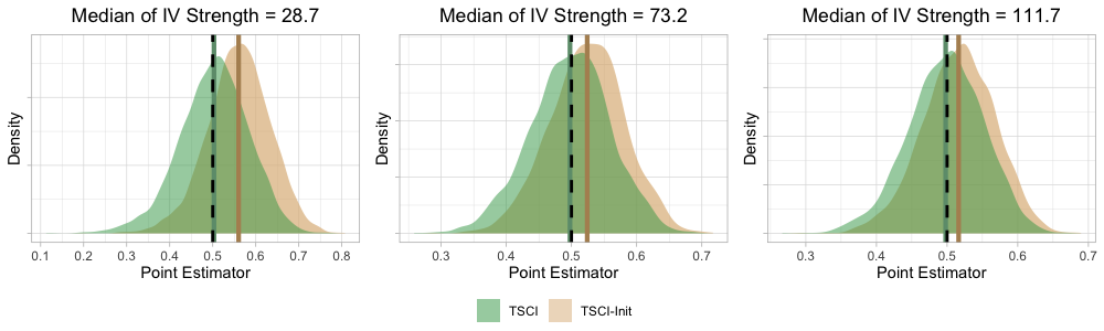
Figure 1: Density plot of TSCI and TSCI-Init estimators (with 500 simulations), which are after and before bias correction, respectively. The three panels from left to right correspond to settings with increasing IV strengths; see Section D.1 in the supplement for details. The black dashed line represents the true value $\beta=0.5$. The green and brown solid lines indicate the means of TSCI and TSCI-Init estimators.

To address this finite-sample bias of $\widehat{\beta}_{\rm init}(V)$, we propose the following bias-corrected estimator,

$$\widehat{\beta}(V)=\frac{{Y}_{\mathcal{A}_{1}}^{\intercal}\mathbf{M}(V){D}_{\mathcal{A}_{1}}}{{D}_{\mathcal{A}_{1}}^{\intercal}\mathbf{M}(V){D}_{\mathcal{A}_{1}}}-\frac{\sum_{i=1}^{n_{1}}[\mathbf{M}(V)]_{ii}\widehat{\delta}_{i}[\widehat{\epsilon}(V)]_{i}}{{{D}_{\mathcal{A}_{1}}^{\intercal}\mathbf{M}(V){D}_{\mathcal{A}_{1}}}}.$$ (19)

with $\widehat{\delta}_{i}=D_{i}-\widehat{f}_{i}$ for $1\leq i\leq n_{1}$ and $\widehat{\epsilon}(V)=P^{\perp}_{V}[Y-D\widehat{\beta}_{\rm init}(V)]$. We show in Figure 1 that our proposal effectively corrects the bias of $\widehat{\beta}_{\rm init}(V)$. Importantly, our proposed bias correction is effective for both homoscedastic and heteroscedastic correlations. We present a simplified bias correction assuming homoscedastic correlation in Section A.10 in the supplement.

Centering at $\widehat{\beta}_{\rm RF}(V)$ defined in (19), we construct the confidence interval

$${\rm CI}(V)=\left(\widehat{\beta}(V)-z_{\alpha/2}\widehat{\rm SE}(V),\widehat{\beta}(V)+z_{\alpha/2}\widehat{\rm SE}(V)\right),$$ (20)

with $z_{\alpha/2}$ denoting the upper $\alpha/2$ quantile of the standard normal distribution and

$$\widehat{\rm SE}(V)=\frac{\sqrt{\sum_{i=1}^{n_{1}}[\widehat{\epsilon}(V)]^{2}_{i}[\mathbf{M}(V){D}_{\mathcal{A}_{1}}]_{i}^{2}}}{{D}_{\mathcal{A}_{1}}^{\intercal}\mathbf{M}(V){D}_{\mathcal{A}_{1}}}\quad\text{with}\quad\widehat{\epsilon}(V)=P^{\perp}_{V}\left[Y-D\widehat{\beta}_{\rm init}(V)\right].$$ (21)

Remark 2

The bias component in (18) results from the correlation between $\epsilon_{i}$ and $\delta_{i}$ for $i\in\mathcal{A}_{1}$. In the regime of many IVs, Angrist et al. (1999) proposed the “leave-one-out” jackknife-type IV estimator, that is, instead of fitting the first stage model with all the data, the treatment model for the $i$-th observation is fitted without using itself. Such an estimator effectively removes the bias for TSLS due to the correlation between $\epsilon_{i}$ and $\delta_{i}$. Our proposed removal of self-prediction is of a similar spirit to the jackknife. However, even after removing the self-prediction, the diagonal of $\mathbf{M}(V)$ is not zero, and hence the correlation between $\epsilon_{i}$ and $\delta_{i}$ still leads to a bias component, which requires the bias correction as in (19).

3.3 Generalized IV strength: detection of under-fitted machine learning

The IV strength is particularly important for identifying the treatment effect stably, and the weak IV is a major concern in practical applications of IV-based methods (Stock et al., 2002; Hansen et al., 2008). With a larger basis set $\mathcal{V}$, the IV strength will generally decrease as the information contained in $\mathcal{V}$ is projected out from the first-stage ML fit. It is crucial to introduce a generalized IV strength measure in consideration of invalid IV forms and the ML algorithm. Similarly to the classical setup, good performance of our proposed TSCI estimator also requires a relatively large generalized IV strength. We introduce a generalized IV strength measure as,

$$\mu(V)\coloneqq{{f}_{\mathcal{A}_{1}}^{\intercal}\mathbf{M}(V){f}_{\mathcal{A}_{1}}}/{\left[\sum_{i\in\mathcal{A}_{1}}{\rm Var}(\delta_{i}\mid X_{i},Z_{i})/n_{1}\right]}.$$ (22)

If ${\rm Var}(\delta_{i}\mid X_{i},Z_{i})=\sigma_{\delta}^{2},$ then $\mu(V)$ is reduced to ${f}_{\mathcal{A}_{1}}^{\intercal}\mathbf{M}(V){f}_{\mathcal{A}_{1}}/\sigma_{\delta}^{2}.$ A sufficiently large strength $\mu(V)$ will guarantee stable point and interval estimators defined in (19) and (20). Hence, we need to check whether $\mu(V)$ is sufficiently large. Since $f$ is unknown, we estimate ${f}_{\mathcal{A}_{1}}^{\intercal}\mathbf{M}(V){f}_{\mathcal{A}_{1}}$ by its sample version ${D}_{\mathcal{A}_{1}}^{\intercal}\mathbf{M}(V){D}_{\mathcal{A}_{1}}$ and estimate $\mu(V)$ by $\widehat{\mu(V)}\coloneqq{{D}_{\mathcal{A}_{1}}^{\intercal}\mathbf{M}(V){D}_{\mathcal{A}_{1}}}/\left[{\|D_{\mathcal{A}_{1}}-\widehat{f}_{\mathcal{A}_{1}}\|_{2}^{2}/n_{1}}\right].$

In Section 4, we show that our point estimator in (19) is consistent when the IV strength $\mu(V)$ is much larger than ${\rm Tr}\left[\mathbf{M}(V)\right]$; see Condition (R2). We now develop a bootstrap test to provide an empirical assessment of this IV strength requirement. Since Rothenberg (1984) and Stock et al. (2002) suggested the concentration parameter being larger than $10$ as being “adequate”, we develop a bootstrap test for $\mu(V)\geq\max\{2{\rm Tr}\left[\mathbf{M}(V)\right],10\}.$ We apply the wild bootstrap method and construct a probabilistic upper bound for the estimation error ${D}_{\mathcal{A}_{1}}^{\intercal}\mathbf{M}(V){D}_{\mathcal{A}_{1}}-{f}_{\mathcal{A}_{1}}^{\intercal}\mathbf{M}(V){f}_{\mathcal{A}_{1}}=2{f}_{\mathcal{A}_{1}}^{\intercal}\mathbf{M}(V){\delta}_{\mathcal{A}_{1}}+{\delta}_{\mathcal{A}_{1}}^{\intercal}\mathbf{M}(V){\delta}_{\mathcal{A}_{1}}.$ For $1\leq i\leq n_{1}$, we define $\widehat{\delta}_{i}=D_{i}-\widehat{f}_{i}$ and compute $\widetilde{\delta}_{i}=\widehat{\delta}_{i}-\bar{\mu}_{\delta}$ with $\bar{\mu}_{\delta}=\frac{1}{n_{1}}\sum_{i=1}^{n_{1}}\widehat{\delta}_{i}.$ For $1\leq l\leq L,$ we generate $\delta^{[l]}_{i}=U^{[l]}_{i}\cdot\widetilde{\delta}_{i}$ for $1\leq i\leq n_{1},$ with $\{U^{[l]}_{i}\}_{1\leq i\leq n_{1}}$ generated as i.i.d. standard normal random variables, and compute $S^{[l]}=\left[{2{f}_{\mathcal{A}_{1}}^{\intercal}\mathbf{M}(V){\delta}^{[l]}+({\delta}^{[l]})^{\intercal}\mathbf{M}(V){\delta}^{[l]}}\right]/\left[{{{\|D_{\mathcal{A}_{1}}-\widehat{f}_{\mathcal{A}_{1}}\|_{2}^{2}/n_{1}}}}\right].$ We use $\mathcal{S}_{\alpha_{0}}(V)$ to denote the upper $\alpha_{0}$ empirical quantile of $\{|S^{[l]}|\}_{1\leq l\leq L}$. We conduct the generalized IV strength test $\widehat{\mu(V)}\geq\max\{2{\rm Tr}\left[\mathbf{M}(V)\right],10\}+{\mathcal{S}_{\alpha_{0}}(V)},$ with ${\mathcal{S}_{\alpha_{0}}(V)}$ being a high probability upper bound for $|\widehat{\mu(V)}-\mu(V)|.$ We use $\alpha_{0}=0.025$ throughout this paper. If the above generalized IV strength test is passed, the IV is claimed to be strong after adjusting for the matrix $V$ defined in (6); otherwise, the IV is claimed to be weak after adjusting for the matrix $V.$ Empirically, we observe reliable inference properties when the estimated generalized IV strength $\widehat{\mu(V)}$ is above 40; see Figure S1 for details.

3.4 Data-dependent selection of $\mathcal{V}$

Our proposed TSCI estimator in (19) requires prior knowledge of the basis set $\mathcal{V}$, which generates the function $g(\cdot)$. In the following, we consider the nested sets of basis functions $\mathcal{V}_{0}\subset\mathcal{V}_{1}\subset\cdots\subset\mathcal{V}_{Q},$ where $Q$ is a positive integer. We devise a data-dependent way to choose the best one among $\{\mathcal{V}_{q}\}_{0\leq q\leq Q}$.

We define $\mathcal{V}_{0}\coloneqq\{\overrightarrow{\bf w}(x)\}$ as the set of basis functions for the valid IV setting. For $q\geq 1$, define $\mathcal{V}_{q}\coloneqq\{v_{1}(\cdot),\cdots,v_{L_{q}}(\cdot),\overrightarrow{\bf w}(x)\}$ as the basis set for different invalid IV forms, where $L_{q}\geq 1$ is the number of basis functions. We present two examples of $\{\mathcal{V}_{q}\}_{1\leq q\leq Q}$ for the single IV setting.

1. Polynomial violation: $\mathcal{V}_{q}=\{z,z^{2},\cdots,z^{q},\overrightarrow{\bf w}(x)\},$ for $1\leq q\leq Q.$

2. Interaction violation: $\mathcal{V}_{1}=\left\{z,z\cdot x_{1},z\cdot x_{2},\cdots,z\cdot x_{p_{x}},\overrightarrow{\bf w}(x)\right\}.$

For $0\leq q\leq Q$, we define the matrix $V_{q}\in\mathbb{R}^{n\times(L_{q}+p_{w})}$ with its $i$-th row defined as $(V_{q})_{i}=\left(v_{1}(Z_{i},X_{i}),\cdots,v_{L_{q}}(Z_{i},X_{i}),W_{i}^{\intercal}\right)^{\intercal}$ with $W_{i}=\overrightarrow{\bf w}(X_{i})$ for $1\leq i\leq n$.

For estimating $q\in\{0,1,\ldots\}$ from data, we proceed as follows. We implement the generalized IV strength test in Section 3.3 and define $Q_{\max}$ as,

$$Q_{\max}\coloneqq\max_{q\geq 0}\left\{q:\widehat{{\mu}(V_{q})}\geq\max\{2{\rm Tr}\left[\mathbf{M}(V_{q})\right],10\}+{\mathcal{S}_{\alpha_{0}}(V_{q})}\right\},$$ (23)

where $\alpha_{0}$ is set at $0.025$ by default. For a larger $q$, we tend to adjust out more information and have relatively weaker IVs. Intuitively, ${Q_{\max}}$ denotes the largest index such that the IVs still have enough strength after adjusting for $V_{q}$. With $Q_{\max},$ we shall choose among $\{V_{q}\}_{0\leq q\leq Q_{\max}}.$ As a remark, when there is no $q\geq 0$ satisfying (23), this corresponds to the weak IV regime. In such a scenario, we shall implement the valid IV estimator and output a warning of weak IV.

For any given $0\leq q\leq Q_{\max},$ we apply the generalized estimator in (19) and construct

$$\widehat{\beta}(V_{q})=\frac{{Y}_{\mathcal{A}_{1}}^{\intercal}\mathbf{M}(V_{q}){D}_{\mathcal{A}_{1}}}{{D}_{\mathcal{A}_{1}}^{\intercal}\mathbf{M}(V_{q}){D}_{\mathcal{A}_{1}}}-\frac{\sum_{i=1}^{n_{1}}[\mathbf{M}(V_{q})]_{ii}\widehat{\delta}_{i}[\widehat{\epsilon}(V_{Q_{\max}})]_{i}}{{{D}_{\mathcal{A}_{1}}^{\intercal}\mathbf{M}(V_{q}){D}_{\mathcal{A}_{1}}}},$$ (24)

with $\widehat{\delta}_{\mathcal{A}_{1}}=D_{\mathcal{A}_{1}}-\widehat{f}_{\mathcal{A}_{1}},$ $\mathbf{M}(\cdot)$ defined in (16), and $\widehat{\epsilon}(\cdot)$ defined in (21).

The selection of the best $V_{q}$ among $\{V_{q}\}_{0\leq q\leq Q_{\max}}$ relies on comparing the estimators $\{\widehat{\beta}(V_{q})\}_{0\leq q\leq Q_{\max}}.$ We start with comparing the difference between the estimators $\widehat{\beta}_{{V}_{q}}$ and $\widehat{\beta}_{{V}_{q^{\prime}}}$ with $0\leq q<q^{\prime}\leq Q_{\max}.$ When $\{g(X_{i},Z_{i})\}_{1\leq i\leq n}$ are well approximated by both $V_{q}$ and $V_{q^{\prime}}$, the approximation errors $R({V}_{q})$ and $R({V}_{q^{\prime}})$ defined in (7) are small and the main difference $\widehat{\beta}(V_{q^{\prime}})-\widehat{\beta}(V_{q})$ is approximately due to the randomness of the errors $\epsilon_{\mathcal{A}_{1}}.$ In such cases. we then have $\widehat{\beta}(V_{q^{\prime}})-\widehat{\beta}(V_{q})$ is approximated centered at zero with the following conditional variance,

$$\widehat{H}(V_{q},V_{q^{\prime}}) =\frac{\sum_{i=1}^{n_{1}}[\widehat{\epsilon}(V_{Q_{\max}})]^{2}_{i}[\mathbf{M}(V_{q^{\prime}}){D}_{\mathcal{A}_{1}}]_{i}^{2}}{[{D}_{\mathcal{A}_{1}}^{\intercal}\mathbf{M}(V_{q^{\prime}})D_{\mathcal{A}_{1}}]^{2}}+\frac{\sum_{i=1}^{n_{1}}[\widehat{\epsilon}(V_{Q_{\max}})]^{2}_{i}[\mathbf{M}(V_{q}){D}_{\mathcal{A}_{1}}]_{i}^{2}}{[{D}_{\mathcal{A}_{1}}^{\intercal}\mathbf{M}(V_{q})D_{\mathcal{A}_{1}}]^{2}}$$ (25)

$$-2\frac{\sum_{i=1}^{n_{1}}[\widehat{\epsilon}(V_{Q_{\max}})]^{2}_{i}[\mathbf{M}(V_{q^{\prime}}){D}_{\mathcal{A}_{1}}]_{i}[\mathbf{M}(V_{q}){D}_{\mathcal{A}_{1}}]_{i}}{[{D}_{\mathcal{A}_{1}}^{\intercal}\mathbf{M}(V_{q^{\prime}})D_{\mathcal{A}_{1}}]\cdot[{D}_{\mathcal{A}_{1}}^{\intercal}\mathbf{M}(V_{q})D_{\mathcal{A}_{1}}]}.$$

Based on the above approximation, we further conduct the following test for whether $\widehat{\beta}(V_{q})$ is significantly different from $\widehat{\beta}(V_{q^{\prime}})$,

$$\mathcal{C}(V_{q},V_{q^{\prime}})={\bf 1}\left({\left|\widehat{\beta}(V_{q})-\widehat{\beta}(V_{q^{\prime}})\right|}/{\sqrt{\widehat{H}(V_{q},V_{q^{\prime}})}}\geq z_{\alpha_{0}}\right),$$ (26)

where $\widehat{\beta}(V_{q})$ and $\widehat{\beta}(V_{q^{\prime}})$ are defined in (24). On the other hand, if the smaller matrix $V_{q}$ does not provide a good approximation of $\{g(Z_{i},X_{i})\}_{1\leq i\leq n}$, the difference $\left|\widehat{\beta}(V_{q})-\widehat{\beta}(V_{q^{\prime}})\right|$ tends to be much larger than the threshold in (26) and hence $\mathcal{C}(V_{q},V_{q^{\prime}})=1$, indicating that $V_{q}$ does not fully generate $\{g(Z_{i},X_{i})\}_{1\leq i\leq n}.$

For $Q_{\max}\geq 2,$ we generalize the pairwise comparison to multiple comparisons. For $0\leq q\leq Q_{\max}-1,$ we compare $\widehat{\beta}(V_{q})$ to any $\widehat{\beta}(V_{q^{\prime}})$ with ${q+1\leq q^{\prime}\leq Q_{\max}}$. Particularly, for $0\leq q\leq Q_{\max}-1,$ we define the test

$$\mathcal{C}(V_{q})={\bf 1}\left(\max_{q+1\leq q^{\prime}\leq Q_{\max}}\left[{\left|\widehat{\beta}(V_{q})-\widehat{\beta}(V_{q^{\prime}})\right|}/{\sqrt{\widehat{H}(V_{q},V_{q^{\prime}})}}\right]\geq\widehat{\rho}\right),$$ (27)

where the thresholding $\widehat{\rho}$ is chosen by the wild bootstrap; see more details in Section A.3 in the supplement. We define $\mathcal{C}(V_{Q_{\max}})=0$ as there is no index larger than ${Q_{\max}}$ that we might compare to. We interpret $\mathcal{C}(V_{q})=0$ as follows: none of the differences $\{|\widehat{\beta}(V_{q})-\widehat{\beta}(V_{q^{\prime}})|\}_{q+1\leq q^{\prime}\leq Q_{\max}}$ is large, indicating that $V_{q}$ (approximately) generates the function $g(\cdot)$ and $\widehat{\beta}(V_{q})$ is a reliable estimator.

We choose the index $\widehat{q}_{c}\in[0,Q_{\max}]$ as $\widehat{q}_{c}=\min_{0\leq q\leq Q_{\max}}\left\{q:\mathcal{C}(V_{q})=0\right\},$ which is the smallest $q$ such that $\mathcal{C}(V_{q})$ is zero. The index $\widehat{q}_{c}$ is interpreted as follows: any matrix containing ${V}_{\widehat{q}_{c}}$ as a submatrix does not lead to a substantially different estimator from that by ${V}_{\widehat{q}_{c}}.$ This provides evidence for ${V}_{\widehat{q}_{c}}$ forming a good approximation of $\{g(Z_{i},X_{i})\}_{1\leq i\leq n}.$ Here, the sub-index “c” represents the comparison as we compare different $\{V_{q}\}_{0\leq q\leq Q_{\max}}$ to choose the best one. Note that $\widehat{q}_{c}$ must exist since $\mathcal{C}(V_{Q_{\max}})=0$ by definition. In finite samples, there are chances that certain violations cannot be detected, especially if the TSCI estimators given by $V_{\widehat{q}_{c}}$ and $V_{\widehat{q}_{c}+1}$ are not significantly different. We propose a more robust choice of the index as $\widehat{q}_{r}=\min\{\widehat{q}_{c}+1,Q_{\max}\},$ where the sub index “r” denotes the robust selection; see the discussion after Theorem 3. We summarize our proposed TSCI estimator in Algorithm 1.

Algorithm 1 TSCI with machine learning

Input: Data $X\in\mathbb{R}^{n\times p_{x}},Z,D,Y\in\mathbb{R}^{n}$; Sets of basis $\{\mathcal{V}_{q}\}_{q\geq 0}$ for approximating $g(\cdot)$;

Output: $\widehat{q}_{c}$ and $\widehat{q}_{r}$; $\widehat{\beta}(V_{\widehat{q}_{c}})$ and $\widehat{\beta}(V_{\widehat{q}_{r}})$; ${\rm CI}(V_{\widehat{q}_{c}})$ and ${\rm CI}(V_{\widehat{q}_{r}})$.

1:Generate matrices $V_{q}$ based on $\mathcal{V}_{q}$ for $q\geq 0$ as in (6);

2:Compute $Q_{\max}$ as in (23) and $\widehat{\epsilon}(V_{Q_{\max}})$ as in (21);

3:Compute $\{\widehat{\beta}(V_{q})\}_{0\leq q\leq Q_{\max}}$ as in (24) and $\{\widehat{H}(V_{q},V_{q^{\prime}})\}_{0\leq q<q^{\prime}\leq Q_{\max}}$ as in (25);

4:if $Q_{\max}\geq 1$ then

5:     Compute $\{\mathcal{C}(V_{q})\}_{0\leq q\leq Q_{\max}-1}$ as in (27);

6:end if

7:Set $\mathcal{C}(V_{Q_{\max}})=0$;

8:Compute $\widehat{q}_{c}=\min\left\{0\leq q\leq Q_{\max}:\mathcal{C}(V_{q})=0\right\}$; $\triangleright$ Comparison selection

9:Compute $\widehat{q}_{r}=\min\{\widehat{q}_{c}+1,Q_{\max}\}$; $\triangleright$ Robust selection

10:Compute $\widehat{\beta}_{\rm RF}(V_{\widehat{q}_{c}})$ and $\widehat{\beta}_{\rm RF}(V_{\widehat{q}_{r}})$ as in (19) with $V=V_{\widehat{q}_{c}},V_{\widehat{q}_{r}},$ respectively;

11:Compute ${\rm CI}_{\rm RF}(V_{\widehat{q}_{c}})$ and ${\rm CI}_{\rm RF}(V_{\widehat{q}_{r}})$ as in (20) with $V=V_{\widehat{q}_{c}},V_{\widehat{q}_{r}},$ respectively.

As a remark, $\mathcal{C}(V_{q},V_{q^{\prime}})$ in (26) can be used to test the IV validity. For any $q^{\prime}\geq 1$, $\mathcal{C}(V_{0},V_{q^{\prime}})=1$ represents that the estimator assuming valid IV is sufficiently different from an estimator allowing for the violation form generated by $V_{q^{\prime}}$, indicating that the valid IV assumption is violated.

3.5 Comparison to Double Machine Learning and Machine Learning IV

We compare our proposed TSCI with the double machine learning (DML) estimator (Chernozhukov et al., 2018) and the machine learning IV (MLIV) estimator (Chen et al., 2023; Liu et al., 2020). As the most significant difference, TSCI provides a valid inference that is robust to a certain class of invalid IVs while DML and MLIV are designed for valid IV regimes only. We focus on the valid IV setting in the following and compare our proposal to DML and MLIV. In the DML framework, Chernozhukov et al. (2018) considered the outcome model $Y_{i}=D_{i}\beta+g(X_{i})+\epsilon_{i}$, which is a special case of our outcome model (3) by assuming valid IVs. The population parameter $\beta$ in DML can be identified through the following expression (Chernozhukov et al., 2018; Emmenegger and Bühlmann, 2021)

$$\beta=\frac{{\mathbf{E}}\left[Y_{i}-{\mathbf{E}}(Y_{i}\mid X_{i})\right][Z_{i}-{\mathbf{E}}(Z_{i}\mid X_{i})]}{{\mathbf{E}}\left[D_{i}-{\mathbf{E}}(D_{i}\mid X_{i})\right][Z_{i}-{\mathbf{E}}(Z_{i}\mid X_{i})]},$$ (28)

where ${\mathbf{E}}(Y_{i}\mid X_{i})$, ${\mathbf{E}}(Z_{i}\mid X_{i}),$ and ${\mathbf{E}}(D_{i}\mid X_{i})$ are fitted by machine learning algorithms.

As a fundamental difference, we apply machine learning algorithms to capture the nonlinear relation between $D_{i}$ and $Z_{i},X_{i}$ while (28) identifies $\beta$ based on the linear association ${\mathbf{E}}\left[D_{i}-{\mathbf{E}}(D_{i}\mid X_{i})\right][Z_{i}-{\mathbf{E}}(Z_{i}\mid X_{i})]$. Due to the first-stage ML, our proposed TSCI estimator is generally more efficient than the DML estimator. On the other hand, we approximate $g(z,x)$ by a set of basis functions, which might provide an inaccurate estimator when the basis functions are misspecified. In contrast, DML learns the conditional mean model by general machine learning algorithms and does not particularly require such a specification of basis functions. We compare the performance of DML and TSCI with valid IVs in Section 5.1 and with invalid IVs in Section 5.3.

Chen et al. (2023); Liu et al. (2020) proposed to use the ML prediction values $\widehat{f}_{\mathcal{A}_{1}}$ in (12) as the IV, referred to as the MLIV in the current paper. With this MLIV, the standard TSLS estimator can be implemented: in the first stage, use OLS regression of $D_{\mathcal{A}_{1}}$ on the MLIV $\widehat{f}_{\mathcal{A}_{1}}$ and the baseline covariates $V_{\mathcal{A}_{1}}$ and construct the predicted value $\widehat{D}_{\mathcal{A}_{1}}=c_{f}\widehat{f}_{\mathcal{A}_{1}}+{V}_{\mathcal{A}_{1}}c_{v}$ with $c_{f}\in\mathbb{R}$ and the vector $c_{v}$ denoting the OLS regression coefficients; in the second stage, use the outcome regression by replacing ${D}_{\mathcal{A}_{1}}$ with $\widehat{D}_{\mathcal{A}_{1}}$. The TSLS estimator with MLIV can then be expressed as

$$\widehat{\beta}_{\rm\texttt{MLIV}}\coloneqq{Y_{\mathcal{A}_{1}}^{\intercal}P_{V_{\mathcal{A}_{1}}}^{\perp}\widehat{D}_{\mathcal{A}_{1}}}/{\widehat{D}_{\mathcal{A}_{1}}^{\intercal}P_{V_{\mathcal{A}_{1}}}^{\perp}\widehat{D}_{\mathcal{A}_{1}}}=\beta+{\epsilon_{\mathcal{A}_{1}}^{\intercal}P_{V_{\mathcal{A}_{1}}}^{\perp}\widehat{f}_{\mathcal{A}_{1}}}/[{c_{f}\cdot\widehat{f}_{\mathcal{A}_{1}}^{\intercal}P_{V_{\mathcal{A}_{1}}}^{\perp}\widehat{f}_{\mathcal{A}_{1}}}].$$ (29)

The last equality of (29) holds by plugging in the outcome model $Y_{i}=D_{i}\beta+V_{i}^{\intercal}\pi+\epsilon_{i}$ and $\widehat{D}_{\mathcal{A}_{1}}=c_{f}\widehat{f}_{\mathcal{A}_{1}}+{V}_{\mathcal{A}_{1}}c_{v}$ and applying the orthogonality between $D_{\mathcal{A}_{1}}-\widehat{D}_{\mathcal{A}_{1}}$ and $\{\widehat{f}_{\mathcal{A}_{1}},{V}_{\mathcal{A}_{1}}\}.$ Note that a dominating term of $\widehat{\beta}_{\rm init}(V)-\beta$ in (17) is ${\widehat{\epsilon}_{\mathcal{A}_{1}}^{\intercal}P^{\perp}_{\widehat{V}_{\mathcal{A}_{1}}}\widehat{f}_{\mathcal{A}_{1}}}/{\widehat{f}_{\mathcal{A}_{1}}^{\intercal}P^{\perp}_{\widehat{V}_{\mathcal{A}_{1}}}\widehat{f}_{\mathcal{A}_{1}}}.$ In comparison, the last term in (29) is roughly inflated by a factor of $1/c_{f}$, appearing due to the additional first-stage regression using the MLIV. When the IV is relatively strong, then this factor $c_{f}$ is around 1, and MLIV and $\widehat{\beta}_{\rm init}(V)$ are of similar performance for valid IV settings. However, in the presence of relatively weak IVs, the coefficient $c_{f}$ in front of $\widehat{f}_{\mathcal{A}_{1}}$ has a large fluctuation due to the weak association between $D_{\mathcal{A}_{1}}$ and $\widehat{f}_{\mathcal{A}_{1}}.$ The weak IV problem deteriorates with the extra first stage regression using the MLIV. This explains why the estimator $\widehat{\beta}_{\rm\texttt{MLIV}}$ in (29) has a much larger bias and standard error than our proposed TSCI estimator in (19) when the IVs are relatively weak; see Section D.2 in the supplementary for the detailed comparison.

4 Theoretical justification

We first establish the asymptotic normality of $\widehat{\beta}(V)$ for a given $V$. To begin with, we present the required conditions. The first assumption is imposed on the regression errors in models (3) and (4) and the data $\{V_{i},f_{i}\}_{1\leq i\leq n}$ with $f_{i}=f(Z_{i},X_{i})$.

1. Conditioning on $Z_{i},X_{i}$, $\epsilon_{i}$ and $\delta_{i}$ are sub-gaussian random variables, that is, there exists a positive constant $K>0$ such that

   $$\sup_{Z_{i},X_{i}}\max\left\{\mathbb{P}(|\epsilon_{i}|>t\mid Z_{i},X_{i}),\mathbb{P}(|\delta_{i}|>t\mid Z_{i},X_{i})\right\}\leq\exp(-{K^{2}t^{2}}/{2}),$$

   with $\sup_{Z_{i},X_{i}}$ denoting the supremum over the support of the density of $Z_{i},X_{i}$. The random variables $\{V_{i},f_{i}\}_{1\leq i\leq n_{1}}$ satisfy $\lambda_{\min}\left(\sum_{i=1}^{n_{1}}V_{i}V_{i}^{\intercal}/n_{1}\right)\geq c$, $\left\|\sum_{i=1}^{n_{1}}V_{i}f_{i}/n_{1}\right\|_{2}\leq C,$ $\max_{1\leq i\leq n_{1}}\{|f_{i}|,\|V_{i}\|_{2}\}\leq C\sqrt{\log n_{1}},$ and $\left\|\sum_{i=1}^{n_{1}}V_{i}[R(V)]_{i}/n_{1}\right\|_{2}\leq C\|R(V)\|_{\infty}$, where $C>0$ and $c>0$ are constants independent of $n$ and $p.$ The matrix $\Omega$ defined in (12) satisfies $\lambda_{\max}(\Omega)\leq C$ for some positive constant $C>0.$

The conditional sub-gaussian assumption is required to establish some concentration results. For the special case where $\epsilon_{i}$ and $\delta_{i}$ are independent of $Z_{i},X_{i},$ it is sufficient to assuming sub-gaussian errors $\epsilon_{i}$ and $\delta_{i}.$ The sub-gaussian conditions on regression errors may be relaxed to moment conditions. The conditions on $V_{i}$ and $f_{i}$ will be automatically satisfied with high probability if ${\mathbf{E}}V_{i}V_{i}^{\intercal}$ is positive definite and $V_{i}$ and $f_{i}$ are sub-gaussian random variables, where the sub-gaussianality conditions on $\{V_{i},f_{i}\}_{1\leq i\leq n}$ may be relaxed to moment conditions. The proof of Lemma 1 in the supplement shows that $\lambda_{\max}(\Omega)\leq 1$ for random forests and deep neural networks.

The second assumption is imposed on the generalized IV strength $\mu(V)$ defined in (22). Throughout the paper, the asymptotics is taken as $n\to\infty.$

1. ${f}_{\mathcal{A}_{1}}^{\intercal}\mathbf{M}(V){f}_{\mathcal{A}_{1}}$ satisfies ${f}_{\mathcal{A}_{1}}^{\intercal}\mathbf{M}(V){f}_{\mathcal{A}_{1}}\rightarrow\infty$ and ${f}_{\mathcal{A}_{1}}^{\intercal}\mathbf{M}(V){f}_{\mathcal{A}_{1}}\gg{\rm Tr}[\mathbf{M}({V})]$, with $\mathbf{M}({V})$ defined in (16).

The above condition is closely related to Condition 1, where ${f}_{\mathcal{A}_{1}}^{\intercal}\mathbf{M}(V){f}_{\mathcal{A}_{1}}$ measures the variability of the estimated $\widehat{f}$ after adjusting for $V$ used to approximate $\{g(Z_{i},X_{i})\}_{1\leq i\leq n}$. Intuitively, a larger value of ${f}_{\mathcal{A}_{1}}^{\intercal}\mathbf{M}(V){f}_{\mathcal{A}_{1}}$ indicates that ${\mathbf{E}}(f(Z_{i},X_{i})-V_{i}^{\intercal}\gamma^{*})^{2}>0$ in Condition 1 holds more plausibly. The generalized IV strength $\mu(V)$ introduced in (22) is proportional to ${f}_{\mathcal{A}_{1}}^{\intercal}\mathbf{M}(V){f}_{\mathcal{A}_{1}}$ when ${\rm Var}(\delta_{i}\mid X_{i},Z_{i})$ is of a constant scale. Our proposed test in Section 3.3 is designed to test whether $\mu(V)$ is sufficiently large for TSCI. For the setting with ${\mathbf{E}}(f(Z_{i},X_{i})-V_{i}^{\intercal}\gamma^{*})^{2}$ in Condition 1 being a positive constant, ${f}_{\mathcal{A}_{1}}^{\intercal}\mathbf{M}(V){f}_{\mathcal{A}_{1}}$ can be of the order $n$, making Condition (R2) a mild assumption.

The following proposition establishes the consistency of $\widehat{\beta}_{\rm init}(V)$ if Conditions (R1) and (R2) hold and the approximation errors $\{R_{i}(V)=g(Z_{i},X_{i})-V^{\intercal}_{i}\pi\}_{1\leq i\leq n}$ are small.

Proposition 1

Consider the models (3) and (4). If Conditions (R1) and (R2) hold and $\|R_{\mathcal{A}_{1}}(V)\|_{2}^{2}\ll{f}_{\mathcal{A}_{1}}^{\intercal}\mathbf{M}(V){f}_{\mathcal{A}_{1}}$, then $\widehat{\beta}_{\rm init}(V)$ defined in (16) satisfies $\widehat{\beta}_{\rm init}(V)\overset{p}{\to}\beta.$

4.1 Improvement with bias correction

In the following, we present the distributional properties of the bias-corrected TSCI estimator $\widehat{\beta}(V)$ defined in (19) and demonstrate the advantage of this extra bias correction step. For establishing the asymptotic normality, we further impose a stronger generalized IV strength condition than (R2).

1. ${f}_{\mathcal{A}_{1}}^{\intercal}[\mathbf{M}(V)]^{2}{f}_{\mathcal{A}_{1}}\rightarrow\infty,$ ${f}_{\mathcal{A}_{1}}^{\intercal}[\mathbf{M}(V)]^{2}{f}_{\mathcal{A}_{1}}\gg\|R(V)\|_{2}^{2},$ and

   $${f}_{\mathcal{A}_{1}}^{\intercal}[\mathbf{M}(V)]^{2}{f}_{\mathcal{A}_{1}}\gg{\max\left\{({\rm Tr}[\mathbf{M}(V)])^{c},\log n\cdot\eta_{n}(V)^{2}\cdot({\rm Tr}[\mathbf{M}(V)])^{2}\right\}},$$

   where $c>1$ is some positive constant and $\eta_{n}(\cdot)$ is defined as

   $$\eta_{n}(V)=\|f_{\mathcal{A}_{1}}-\widehat{f}_{\mathcal{A}_{1}}\|_{\infty}+\left(|\beta-\widehat{\beta}_{\rm init}(V)|+\|R(V)\|_{\infty}+{{\frac{\log n}{\sqrt{n}}}}\right)(\sqrt{\log n}+\|f_{\mathcal{A}_{1}}-\widehat{f}_{\mathcal{A}_{1}}\|_{\infty}).$$ (30)

The above condition can be viewed as requiring the IV to be sufficiently strong, where ${f}_{\mathcal{A}_{1}}^{\intercal}[\mathbf{M}(V)]^{2}{f}_{\mathcal{A}_{1}}$ can be viewed as another measure of IV strength. If the treatment model is fitted with neural network, we have ${f}_{\mathcal{A}_{1}}^{\intercal}[\mathbf{M}(V)]^{2}{f}_{\mathcal{A}_{1}}={f}_{\mathcal{A}_{1}}^{\intercal}\mathbf{M}(V){f}_{\mathcal{A}_{1}}$. For random forests, we only have ${f}_{\mathcal{A}_{1}}^{\intercal}[\mathbf{M}(V)]^{2}{f}_{\mathcal{A}_{1}}\leq{f}_{\mathcal{A}_{1}}^{\intercal}\mathbf{M}(V){f}_{\mathcal{A}_{1}}$. $\eta_{n}(V)$ defined in (30) depends on the accuracy of the ML prediction model $\widehat{f}.$ We have $\eta_{n}(V)\rightarrow 0$ if $\|f_{\mathcal{A}_{1}}-\widehat{f}_{\mathcal{A}_{1}}\|_{\infty}\rightarrow 0$, $\widehat{\beta}_{\rm init}(V)\overset{p}{\to}\beta$, and $\|R(V)\|_{\infty}\rightarrow 0$. However, even for inconsistent $\widehat{f}$, $\eta_{n}(V)$ is of a smaller order of magnitude than $\sqrt{\log n}$ as long as $\|f_{\mathcal{A}_{1}}-\widehat{f}_{\mathcal{A}_{1}}\|_{\infty}$ is of a constant scale.

The following theorem establishes the asymptotic normality of the TSCI estimator.

Theorem 1

Consider the models (3) and (4). Suppose that Condition (R1), (R2-I) hold and

$$\frac{\max_{1\leq i\leq n_{1}}\sigma_{i}^{2}\cdot\left[\mathbf{M}(V){f}_{\mathcal{A}_{1}}\right]_{i}^{2}}{\sum_{i=1}^{n_{1}}\sigma_{i}^{2}\cdot\left[\mathbf{M}(V){f}_{\mathcal{A}_{1}}\right]_{i}^{2}}\rightarrow 0\quad\text{with}\quad\sigma_{i}^{2}={\mathbf{E}}(\epsilon_{i}^{2}\mid Z_{i},X_{i}).$$ (31)

Then $\widehat{\beta}(V)$ defined in (19) satisfies

$$\frac{1}{{\rm SE}(V)}\left(\widehat{\beta}(V)-\beta\right)\overset{d}{\to}N(0,1),\quad\text{with}\quad{\rm SE}(V)=\frac{\sqrt{\sum_{i=1}^{n_{1}}\sigma^{2}_{i}[\mathbf{M}(V){f}_{\mathcal{A}_{1}}]_{i}^{2}}}{{f}_{\mathcal{A}_{1}}^{\intercal}\mathbf{M}(V){f}_{\mathcal{A}_{1}}}.$$

If $\widehat{\rm SE}(V)$ used in (20) satisfies $\widehat{\rm SE}(V)/{\rm SE}(V)\overset{p}{\to}1,$ then the confidence interval ${\rm CI}(V)$ in (20) satisfies $\liminf_{n\rightarrow\infty}\mathbb{P}(\beta\in{\rm CI}(V))=1-\alpha.$

We emphasize that the validity of our proposed confidence interval does not require the ML prediction model $\widehat{f}$ to be a consistent estimator of $f$. Particularly, Condition (R2) and (R2-I) can be plausibly satisfied as long as the ML algorithms capture enough association between the treatment and the IVs. The condition (31) is imposed such that not a single entry of the vector $\mathbf{M}(V){f}_{\mathcal{A}_{1}}$ dominates all other entries, which is needed for verifying the Linderberg condition. The standard error ${\rm SE}(V)$ relies on the generalized IV strength for a given matrix $V$. If ${f}_{\mathcal{A}_{1}}^{\intercal}\mathbf{M}(V){f}_{\mathcal{A}_{1}}/n_{1}$ is of constant order, then ${\rm SE}(V)\lesssim{1}/{\sqrt{n}}.$ A larger matrix $V$ will generally lead to a larger ${\rm SE}(V)$ because ${f}_{\mathcal{A}_{1}}^{\intercal}\mathbf{M}(V){f}_{\mathcal{A}_{1}}$ decreases after adjusting for more information contained in $V$. The consistency of $\widehat{\rm SE}(V)$ is presented in Lemma 2 in the supplement.

We now explain the effectiveness of the bias correction for the homoscedastic setting with ${\rm Cov}(\epsilon_{i},\delta_{i}\mid Z_{i},X_{i})={\rm Cov}(\epsilon_{i},\delta_{i})$. For the initial estimator $\widehat{\beta}_{\rm init}(V),$ we can establish that $\frac{1}{{\rm SE}(V)}\left(\widehat{\beta}_{\rm init}(V)-\beta\right)={\mathcal{G}}(V)+\widetilde{\mathcal{E}}(V),$ where ${\mathcal{G}}(V)\overset{d}{\to}N(0,1)$ and

$$\left|\widetilde{\mathcal{E}}(V)\right|\leq\frac{{\rm Cov}(\epsilon_{i},\delta_{i})\cdot{\rm Tr}[\mathbf{M}(V)]+\|R(V)\|_{2}}{\sqrt{{f}_{\mathcal{A}_{1}}[\mathbf{M}(V)]^{2}{f}_{\mathcal{A}_{1}}}}+\frac{\sqrt{{\rm Tr}([\mathbf{M}({V})]^{2})}}{({f}_{\mathcal{A}_{1}}[\mathbf{M}(V)]^{2}{f}_{\mathcal{A}_{1}})^{c_{0}}},$$ (32)

for some positive constant $c_{0}>0.$ Our proposed bias-corrected estimator $\widehat{\beta}(V)$ is effective in reducing the bias component $\widetilde{\mathcal{E}}(V).$ Particularly, Theorem 4 in Section A.10 in the supplement establishes that the term ${\rm Cov}(\epsilon_{i},\delta_{i})\cdot{\rm Tr}[\mathbf{M}(V)]/\sqrt{{f}_{\mathcal{A}_{1}}[\mathbf{M}(V)]^{2}{f}_{\mathcal{A}_{1}}}$ in (32) is reduced to $\eta_{n}(V)\cdot{\rm Tr}[\mathbf{M}(V)]/\sqrt{{f}_{\mathcal{A}_{1}}[\mathbf{M}(V)]^{2}{f}_{\mathcal{A}_{1}}}$. If $\eta_{n}(V)\rightarrow 0$, which can be achieved for a consistent ML prediction $\widehat{f}$, the bias-corrected TSCI estimator effectively reduces the finite-sample or higher-order bias. However, even if $\widehat{f}_{\mathcal{A}_{1}}$ is inconsistent with $\|f_{\mathcal{A}_{1}}-\widehat{f}_{\mathcal{A}_{1}}\|_{2}\lesssim\sqrt{n}$, the bias correction will not lead to a worse estimator.

4.2 Guarantee for Algorithm 1

We now justify the validity of the confidence interval from the TSCI Algorithm 1, which is based on the asymptotic normality of $\widehat{\beta}(V_{\widehat{q}})$ with a data-dependent index $\widehat{q}$. The property of $\widehat{q}$ relies on a careful analysis of the difference $\widehat{\beta}(V_{q})-\widehat{\beta}(V_{q^{\prime}})$ for $0\leq q<q^{\prime}\leq Q_{\max}$.

We start with the setting where both $V_{q}$ and $V_{q^{\prime}}$ provide good approximations to $\{g(Z_{i},X_{i})\}_{1\leq i\leq n},$ leading to sufficiently small $\|R(V_{q})\|_{2}$ and $\|R(V_{q^{\prime}})\|_{2}$. In this case, the dominating component of $\widehat{\beta}(V_{q})-\widehat{\beta}(V_{q^{\prime}})$ is $S^{\intercal}\epsilon_{\mathcal{A}_{1}}$ with

$$S=\left(\frac{1}{f_{\mathcal{A}_{1}}^{\intercal}\mathbf{M}(V_{q^{\prime}})f_{\mathcal{A}_{1}}}\mathbf{M}(V_{q^{\prime}})-\frac{1}{f_{\mathcal{A}_{1}}^{\intercal}\mathbf{M}(V_{q})f_{\mathcal{A}_{1}}}\mathbf{M}(V_{q})\right)f_{\mathcal{A}_{1}}\in\mathbb{R}^{n_{1}}.$$ (33)

Conditioning on the data in $\mathcal{A}_{2}$ and $\{X_{i},Z_{i}\}_{i\in\mathcal{A}_{1}},$ $S^{\intercal}\epsilon_{\mathcal{A}_{1}}$ is of zero mean and variance

$${H}(V_{q},V_{q^{\prime}})=\frac{\sum_{i=1}^{n_{1}}\sigma_{i}^{2}[\mathbf{M}(V_{q^{\prime}}){f}_{\mathcal{A}_{1}}]_{i}^{2}}{[{f}_{\mathcal{A}_{1}}^{\intercal}\mathbf{M}(V_{q^{\prime}})f_{\mathcal{A}_{1}}]^{2}}+\frac{\sum_{i=1}^{n_{1}}\sigma_{i}^{2}[\mathbf{M}(V_{q}){f}_{\mathcal{A}_{1}}]_{i}^{2}}{[{f}_{\mathcal{A}_{1}}^{\intercal}\mathbf{M}(V_{q})f_{\mathcal{A}_{1}}]^{2}}-2\frac{\sum_{i=1}^{n_{1}}\sigma_{i}^{2}[\mathbf{M}(V_{q^{\prime}}){f}_{\mathcal{A}_{1}}]_{i}[\mathbf{M}(V_{q}){f}_{\mathcal{A}_{1}}]_{i}}{[{f}_{\mathcal{A}_{1}}^{\intercal}\mathbf{M}(V_{q^{\prime}})f_{\mathcal{A}_{1}}]\cdot[{f}_{\mathcal{A}_{1}}^{\intercal}\mathbf{M}(V_{q})f_{\mathcal{A}_{1}}]},$$ (34)

with $\sigma_{i}^{2}={\mathbf{E}}(\epsilon_{i}^{2}\mid Z_{i},X_{i}).$ The following condition requires that the variance of $S^{\intercal}f_{\mathcal{A}_{1}}$ dominates other components of $\widehat{\beta}(V_{q})-\widehat{\beta}(V_{q^{\prime}}),$ which are mainly finite-sample approximation errors.

1. The variance $H(V_{q},V_{q^{\prime}})$ in (34) satisfies

   $$\sqrt{H(V_{q},V_{q^{\prime}})}\gg\max_{V\in\{V_{q},V_{q^{\prime}}\}}\left\{\frac{1}{\mu(V)}\left[1+(1+\sqrt{\log n}\cdot\eta_{n}(V_{Q_{\max}}))\cdot{\rm Tr}[\mathbf{M}(V)]\right]\right\},$$

   with $\eta_{n}(\cdot)$ defined in (30). There exists $c>0$ such that ${\rm Var}(\delta_{i}\mid Z_{i},X_{i})\geq c.$

When the first stage is fitted with the basis method or neural network and ${\rm Var}(\epsilon_{i}\mid Z_{i},X_{i})=\sigma_{\epsilon}^{2},{\rm Var}(\delta_{i}\mid Z_{i},X_{i})=\sigma_{\delta}^{2},$ we have $H(V_{q},V_{q^{\prime}})=\sigma_{\epsilon}^{2}\left({1}/{f^{\intercal}\mathbf{M}({V}_{q^{\prime}})f}-{1}/{f^{\intercal}\mathbf{M}({V}_{q})f}\right)$ and ${\mu(V_{q})}={f^{\intercal}\mathbf{M}({V}_{q})f}/\sigma_{\delta}^{2}$ for $q\leq q^{\prime}.$ If we assume that $f^{\intercal}\mathbf{M}({V}_{q^{\prime}})f=c_{*}f^{\intercal}\mathbf{M}({V}_{q})f$ for some $0<c_{*}<1,$ we have $H(V_{q},V_{q^{\prime}})=\frac{1-c_{*}}{c_{*}}\frac{\sigma_{\epsilon}^{2}}{\sigma_{\delta}^{2}}\mu(V_{q}).$ In this case, Condition (R3) is satisfied if $\mu(V_{q})\gg({\rm Tr}[\mathbf{M}(V_{q})])^{2}$ and $\mu(V_{q^{\prime}})\gg({\rm Tr}[\mathbf{M}(V_{q^{\prime}})])^{2}$ up to some polynomial order of $\log n$. In this case, Condition (R3) is slightly stronger than Condition (R2-I).

The following theorem establishes the asymptotic normality of $\widehat{\beta}(V_{q})-\widehat{\beta}(V_{q^{\prime}})$ under the null setting where both $R(V_{q})$ and $R(V_{q^{\prime}})$ are small.

Theorem 2

Consider the model (3) and (4). Suppose that (R1) and (R3) hold, (R2) holds for $V\in\{V_{q},V_{q^{\prime}}\}$, and $S$ defined in (33) satisfies $\max_{i\in\mathcal{A}_{1}}{S_{i}^{2}}/(\sum_{i\in\mathcal{A}_{1}}S_{i}^{2})\rightarrow 0$. If $\sqrt{H(V_{q},V_{q^{\prime}})}\gg\max_{V\in\{V_{q},V_{q^{\prime}}\}}{\|R(V)\|_{2}}/{\sqrt{\mu(V)}},$ then $\left(\widehat{\beta}(V_{q})-\widehat{\beta}(V_{q^{\prime}})\right)/{\sqrt{H(V_{q},V_{q^{\prime}})}}\overset{d}{\to}N(0,1),$ with $\widehat{\beta}(\cdot)$ and $H(V_{q},V_{q^{\prime}})$ defined in (24) and (34), respectively.

For small approximation errors $\|R(V_{q})\|_{2}$ and $\|R(V_{q^{\prime}})\|_{2}$, the condition $\sqrt{H(V_{q},V_{q^{\prime}})}\gg\max_{V\in\{V_{q},V_{q^{\prime}}\}}{\|R(V)\|_{2}}/{\sqrt{\mu(V)}}$ holds. In this case, Theorem 2 establishes that the difference $\widehat{\beta}(V_{q})-\widehat{\beta}(V_{q^{\prime}})$ is centered at zero and has an asymptotic normal distribution.

We now move on to the case that at least one of $V_{q}$ and $V_{q^{\prime}}$ does not approximate $\{g(Z_{i},X_{i})\}_{1\leq i\leq n}$ well. In this case, Theorem 2 does not hold and we establish Theorem 5 in the supplement that $(\widehat{\beta}(V_{q})-\widehat{\beta}(V_{q^{\prime}}))/{\sqrt{H(V_{q},V_{q^{\prime}})}}$ is centered at

$$\mathcal{L}_{n}(V_{q},V_{q^{\prime}})=\frac{1}{\sqrt{H(V_{q},V_{q^{\prime}})}}\left(\frac{D_{\mathcal{A}_{1}}^{\intercal}\mathbf{M}(V_{q})[R(V_{q})]_{\mathcal{A}_{1}}}{{D}^{\intercal}_{\mathcal{A}_{1}}\mathbf{M}(V_{q})D_{\mathcal{A}_{1}}}-\frac{D_{\mathcal{A}_{1}}^{\intercal}\mathbf{M}(V_{q^{\prime}})[R(V_{q^{\prime}})]_{\mathcal{A}_{1}}}{{D}^{\intercal}_{\mathcal{A}_{1}}\mathbf{M}(V_{q^{\prime}})D_{\mathcal{A}_{1}}}\right).$$ (35)

To simultaneously quantify the errors of $\{\widehat{\beta}(V_{q})-\widehat{\beta}(V_{q^{\prime}})\}_{0\leq q<q^{\prime}\leq Q_{\max}},$ we define the $\alpha_{0}$ quantile for the maximum of multiple random error components in (33),

$$\mathbb{P}\left(\max_{0\leq q<q^{\prime}\leq Q_{\max}}\frac{1}{\sqrt{{H}(V_{q},V_{q^{\prime}})}}\left|\frac{f_{\mathcal{A}_{1}}^{\intercal}\mathbf{M}(V_{q^{\prime}})\epsilon_{\mathcal{A}_{1}}}{{f}_{\mathcal{A}_{1}}^{\intercal}\mathbf{M}(V_{q^{\prime}})f_{\mathcal{A}_{1}}}-\frac{f_{\mathcal{A}_{1}}^{\intercal}\mathbf{M}(V_{q})\epsilon_{\mathcal{A}_{1}}}{f_{\mathcal{A}_{1}}^{\intercal}\mathbf{M}(V_{q})f_{\mathcal{A}_{1}}}\right|\geq\rho(\alpha_{0})\right)=\alpha_{0}.$$ (36)

We introduce the following condition for accurate selection among $\{\mathcal{V}_{q}\}_{0\leq q\leq Q}.$

1. For $\mathcal{V}_{0}\subset\mathcal{V}_{1}\subset\cdots\subset\mathcal{V}_{Q}$ and corresponding matrices $\{{V}_{q}\}_{0\leq q\leq Q}$, there exists $q^{*}\in\{0,1,2,\cdots,Q\}$ such that $q^{*}\leq Q_{\max}$ and $R(V_{q^{*}})=0$ with $Q_{\max}$ defined in (23). For any integer $q\in[0,q^{*}-1],$ there exists an integer $q^{\prime}\in[q+1,q^{*}]$ such that

   $$\mathcal{L}_{n}(V_{q},V_{q^{\prime}})\geq A\rho({\alpha_{0}})\quad\text{with}\quad A>2,$$ (37)

   where $\mathcal{L}_{n}(V_{q},V_{q^{\prime}})$ is defined in (35) and $\rho({\alpha_{0}})$ is defined in (36).

The above condition ensures that there exists $\mathcal{V}_{q^{*}}$ such that the function $g$ is well approximated by the column space of $V_{q^{*}}$. The well-separation condition (37) is interpreted as follows: if $g$ is not well approximated by the column space of $V_{q}$, then the estimation bias of $\widehat{\beta}(V_{q})$ is larger than the uncertainty $\rho({\alpha_{0}})$ due to the multiple random error components. Note that $\mathcal{L}_{n}(V_{q},V_{q^{*}})$ defined in (35) is a measure of the bias of $\widehat{\beta}(V_{q}).$

The following theorem guarantees the coverage property for the CIs corresponding to $V_{\widehat{q}_{c}}$ and $V_{\widehat{q}_{r}}$ in Algorithm 1.

Theorem 3

Consider the model (3) and (4). Suppose that Conditions (R1) and (R4) hold, Condition (R2-I) holds for $V\in\{V_{q}\}_{0\leq q\leq Q_{\max}}$, Condition (R3) holds for any $0\leq q<q^{\prime}\leq Q_{\max}$, $\widehat{H}(V_{q},V_{q^{\prime}})/H(V_{q},V_{q^{\prime}})\overset{p}{\to}1$, and $\widehat{\rho}/\rho(\alpha_{0})\overset{p}{\to}1$ with $\widehat{\rho}$ used in (27) and $\rho(\alpha_{0})$ defined in (36) respectively. Our proposed CI in Algorithm 1 satisfies $\liminf_{n\rightarrow\infty}\mathbb{P}\left[\beta\in{\rm CI}(V_{\widehat{q}})\right]\geq 1-\alpha-2\alpha_{0}$ with $\widehat{q}=\widehat{q}_{c}$ or $\widehat{q}_{r}$ where $\alpha_{0}$ is used in (36).

The condition (37) of (R4) is critical to guarantee the selection consistency $\widehat{q}_{c}=q^{*}$, ensuring that ${\rm CI}(V_{\widehat{q}_{c}})$ achieves the desired coverage. However, in finite samples, we may make mistakes in conducting the selection among $\{V_{q}\}_{0\leq q\leq Q_{\max}}.$ The selection method $\widehat{q}_{r}$ is more robust in the sense that statistical inference based on $V_{\widehat{q}_{r}}$ is still valid even if we cannot separate $V_{q^{*}-1}$ and $V_{q^{*}}.$ To achieve the uniform inference without requiring the well-separation condition (37), we may simply apply TSCI with $\mathcal{V}_{Q_{\max}}$. However, such a confidence interval might be conservative by adjusting for a large $V_{Q_{\max}}.$

5 Simulation studies

In Section 5.1, we consider the valid IV settings and compare our proposal to the DML estimator proposed in Chernozhukov et al. (2018). In Sections 5.2 and 5.3, we demonstrate our proposal for general invalid IV settings and also compare it with the DML estimator. In Section D.3 in the supplement, we further consider multiple IVs settings and compare TSCI with existing methods based on the majority rule. We compute all measures using 500 simulations throughout the numerical studies. The code for replicating the numerical results is available at https://github.com/zijguo/TSCI-Replication.

5.1 Comparison with DML in valid IV settings

We focus on the valid IV settings and illustrate the advantages and limitations of both TSCI and DML. We adopt the data generative setting used in the R package dmlalg (Emmenegger, 2021) and implement DML by the R package DoubleML (Bach et al., 2021). We set the sample size as $n=3000$ and generate the baseline covariate $X_{i}\in\mathbb{R}$ following the uniform distribution on $[-\pi,\pi]$. Conditioning on $X_{i}$, we generate the IV $Z_{i}$ and the hidden confounder $H_{i}$ following $Z_{i}\mid X_{i}\sim N(3\cdot\tanh(2X_{i}-1),1)$ and $H_{i}\mid X_{i}\sim N(2\cdot\sin(X_{i}),1)$, respectively. We generate the outcome $Y_{i}$ and treatment $D_{i}$ using the SEM in (9). Particularly, we generate the outcome $Y_{i}$ following $Y_{i}=D_{i}+X_{i}^{2}/2-3\cdot\cos(\pi H_{i}/4)+e_{i,2}$ and consider the following two treatment models,

• Setting S1: $D_{i}=-a\cdot|Z_{i}|-2\cdot\tanh(X_{i})-H_{i}+e_{i,1},$

• Setting S2: $D_{i}=a\cdot Z_{i}^{2}/2-2\cdot\tanh(X_{i})-H_{i}+e_{i,1},$

where $a$ controls the nonlinearity of the treatment model and strength of the IV and $e_{i,1}\sim N(0,1)$ and $e_{i,2}\sim N(0,1)$ are independent noises. Note that a larger value of $a$ in the treatment model leads to a more nonlinear dependence between $D_{i}$ and $Z_{i}$. The treatment model and the outcome model are consistent to (4) and (3) with $\delta_{i}$ and $\epsilon_{i}$ being composed of a hidden confounder term and an independent random noise.

In addition to the above two settings, we consider another setting where $g(X_{i})$ in the outcome model is more complicated. We set $p_{x}=5$ and for $1\leq i\leq n$, we generate $\{X_{i,j}\}_{1\leq j\leq p_{x}}$ which are independently distributed, and each of them follows a uniform distribution on $[-1,1]$. We generate $Z_{i}$ and $H_{i}$ following $Z_{i}\mid X_{i}\sim N(3\cdot\tanh(2X_{i,1}-1),1)$ and $H_{i}\mid X_{i}\sim N(2\cdot\sin(X_{i,1}),1)$. We generate $\{D_{i},Y_{i}\}_{1\leq i\leq n}$ following

• Setting S3: $D_{i}=b\cdot Z_{i}+\sin(2\pi Z_{i})+3/2\cdot\cos(2\pi Z_{i})-1/5\cdot\sum_{j=1}^{p_{x}}X_{i,j}-1/2\cdot H_{i}+e_{i,1}$ and $Y_{i}=D_{i}/2+g(X_{i})-\cos(\pi H_{i}/4)+e_{i,2}$ with $g(X_{i})=\sum_{1\leq j\neq k\leq p_{x}}X_{i,j}X_{i,k}$,

where the value of $b$ controls the linear association strength in Setting S3. We implement Algorithm 1 with random forests by specifying a collection of basis functions for $g(x)$. Since the IV is valid here, we use the set of basis functions $\mathcal{V}_{0}=\{1,\overrightarrow{\bf b}_{1}(x_{1}),\cdots,\overrightarrow{\bf b}_{p_{x}}(x_{p_{x}})\}$ with $\overrightarrow{\bf b}_{j}(x_{j})$ denoting the B-spline basis with 5 knots of $x_{j}$ for $1\leq j\leq p_{x}$.

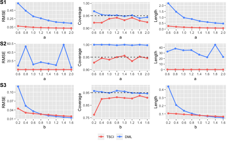
Figure 2: Comparison of DML and TSCI in terms of RMSE, CI coverage, and length under Settings S1, S2, and S3. The larger value of the constant $a$ in Settings S1 and S2 stands for a higher nonlinearity level in the treatment model, and the larger value of $b$ in Setting S3 for a higher linearity level. In addition, a larger value of $a$ and $b$ indicate larger generalized IV strength.

In Figure 2, we compare DML and TSCI under Settings S1, S2, and S3. In the top two panels, TSCI achieves the desired coverage level in Settings S1 and S2. Even though DML achieves desired coverage in setting S1, the RMSE and CI length of DML is uniformly larger than those of our proposed TSCI. As discussed in Section 3.5, this happens since DML only uses the linear association in the treatment model while TSCI can increase the IV strength by applying ML algorithms to fit nonlinear treatment models. We have designed setting S2 as a less favorable setting for DML, where the linear association between the treatment and IV is nearly zero but the nonlinear association is strong. Consequently, the CI length and RMSE of the DML procedure is much larger than our proposed TSCI. In Setting S3, TSCI does not show the advantage over DML and has an under-coverage problem. This is caused by the estimation bias due to the misspecification of $g(x)$ in the outcome model. DML is not exposed to such bias because it uses ML algorithms to fit $E(Y_{i}\mid X_{i})$. We also implement TSLS in Settings S1, S2 and S3, but we do not include it in the figures because it has low coverage due to misspecification of nonlinear $g(x)$.

5.2 TSCI with invalid IVs

We now demonstrate our TSCI method under the general setting with possibly invalid IVs. In the following, we focus on the continuous treatment and will investigate the performance of TSCI for binary treatment in Section D.5 in the supplement. We generate $X^{*}_{i}\in\mathbb{R}^{p_{x}+1}$ following a multivariate normal distribution with zero mean and covariance matrix $\Sigma$ where $\Sigma_{ij}=0.5^{|i-j|}$ for $1\leq i,j\leq p_{x}+1$. With $\Phi$ denoting the standard normal cumulative distribution function, we define $X_{ij}=\Phi(X^{*}_{ij})$ for $1\leq j\leq p_{x}.$ We generate a continuous IV as $Z_{i}=4(\Phi(X^{*}_{i,p_{x}+1})-0.5)\in(-2,2)$.

We consider the following two conditional mean models for the treatment,

• Setting B1: $f(Z_{i},X_{i})=-\frac{25}{12}+Z_{i}+Z_{i}^{3}/3+Z_{i}\cdot(a\cdot\sum_{j=1}^{5}X_{ij})-\frac{3}{10}\cdot\sum_{j=1}^{p}X_{ij},$

• Setting B2: $f(Z_{i},X_{i})=\sin(2\pi Z_{i})+\frac{3}{2}\cos(2\pi Z_{i})+Z_{i}\cdot(a\cdot\sum_{j=1}^{5}X_{ij})-\frac{3}{10}\cdot\sum_{j=1}^{p}X_{ij}.$

The value of the constant $a$ controls the interaction strength between $Z_{i}$ and the first five variables of $X_{i}$, and when $a=0$, the interaction term disappears. We vary $a$ across $\{0,0.5,1\}$ and $n$ across $\{1000,3000,5000\}$ to observe the performance.

We consider the outcome model (3) with two forms of $g(Z_{i},X_{i})$: (a)Vio=1: $g(Z_{i},X_{i})=Z_{i}+1/5\cdot\sum_{j=1}^{p_{x}}X_{ij}$; (b)Vio=2: $g(Z_{i},X_{i})=Z_{i}+Z_{i}^{2}-1+1/5\cdot\sum_{j=1}^{p_{x}}X_{ij}$. We set the errors $\{(\delta_{i},\epsilon_{i})^{\intercal}\}_{1\leq i\leq n}$ as heteroscedastic following Bekker and Crudu (2015): for $1\leq i\leq n,$ generate $\delta_{i}\sim N(0,Z_{i}^{2}+0.25)$ and $\epsilon_{i}=0.6\delta_{i}+\sqrt{{[1-0.6^{2}]}/[0.86^{4}+1.38072^{2}]}(1.38072\cdot\tau_{1,i}+0.86^{2}\cdot\tau_{2,i}),$ where conditioning on $Z_{i}$, $\tau_{1,i}$ and $\tau_{2,i}$ are generated to be independent of $\delta_{i}$, with $\tau_{1,i}\sim N(0,Z_{i}^{2}+0.25)$ and $\tau_{2,i}\sim N(0,1).$

We shall implement TSCI with random forests as detailed in Algorithm 1. Since the IV is possibly invalid, we consider four possible basis sets $\{\mathcal{V}_{q}\}_{0\leq q\leq 3}$ to approximate $g(z,x)$, where $\mathcal{V}_{0}=\{\overrightarrow{\bf w}(x)\}$ and $\mathcal{V}_{q}=\{z,\cdots,z^{q},\overrightarrow{\bf w}(x)\}$ for $1\leq q\leq 3$ with $\overrightarrow{\bf w}(x)=\{1,x_{1},\cdots,x_{p_{x}}\}$. Our proposed TSCI is designed to choose the best $\mathcal{V}_{q}$.

As “naive” benchmarks, we compare TSCI with three different random forests based methods in the oracle setting, where the best $\mathcal{V}_{q}$ is known a priori. In particular, RF-Init denotes the TSCI estimator without bias correction; RF-Full is to implement TSCI without data-splitting; RF-Plug is the estimator of directly plugging the ML fitted treatment in the outcome model, as a naive generalization of TSLS. We give the detailed expressions of these three estimators and their CIs in Section A.2 in the supplement.

			TSCI-RF				Proportions of selection				TSLS	Other RF(oracle)
vio	a	n	Oracle	Comp	Robust	Invalidity	$\widehat{q}_{c}=0$	$\widehat{q}_{c}=1$	$\widehat{q}_{c}=2$	$\widehat{q}_{c}=3$		Init	Plug	Full
1	0.0	1000	0.91	0.01	0.01	0.01	0.99	0.01	0.00	0.00	0.00	0.80	0.38	0.01
		3000	0.92	0.92	0.92	1.00	0.00	0.84	0.16	0.00	0.00	0.91	0.64	0.00
		5000	0.91	0.92	0.93	1.00	0.00	0.85	0.15	0.00	0.00	0.89	0.74	0.00
	0.5	1000	0.91	0.23	0.25	0.24	0.76	0.24	0.01	0.00	0.00	0.84	0.56	0.02
		3000	0.95	0.94	0.94	1.00	0.00	0.97	0.02	0.01	0.00	0.91	0.43	0.00
		5000	0.92	0.92	0.91	1.00	0.00	0.98	0.01	0.01	0.00	0.88	0.09	0.00
	1.0	1000	0.96	0.92	0.92	0.95	0.05	0.93	0.01	0.00	0.00	0.91	0.52	0.08
		3000	0.94	0.94	0.95	1.00	0.00	0.99	0.01	0.00	0.00	0.92	0.00	0.00
		5000	0.94	0.94	0.94	1.00	0.00	0.98	0.02	0.01	0.00	0.92	0.00	0.00

Table 1: Coverage for Setting B1 with Vio=1. The columns indexed with “TSCI-RF” correspond to our proposed TSCI with random forests, where the columns indexed with “Oracle”, “Comp” and “Robust” correspond to the estimators with $\mathcal{V}_{q}$ selected by the oracle knowledge, the comparison method, and the robust method. The column indexed with “Invalidity” reports the proportion of detecting the proposed IV as invalid. The columns indexed with “Proportions of selection” reports the proportions of basis sets $\mathcal{V}_{q}$ for $0\leq q\leq 3$ selected by TSCI-RF. The column indexed with “TSLS” corresponds to the TSLS estimator. The columns indexed with “Init”, “Plug”, and “Full” correspond to the RF estimators without bias correction, the plug-in RF estimator and the no data-splitting RF estimator, with the oracle knowledge of the best $\mathcal{V}_{q}$.

In Table 1, we compare the coverage properties of our proposed TSCI, TSLS, and the above three random forests based methods with Vio=1 in the outcome model. We observe that TSLS fails to have desired coverage probability 95% due to the existence of invalid IV; furthermore, RF-Full and RF-Plug have coverages far below 95% and RF-Init has slightly lower coverage due to the finite-sample bias. In contrast, our proposed TSCI achieves the desired coverage with a relatively strong interaction or large sample size. This is mainly due to its correct selection of $\mathcal{V}_{q}$ in those settings. In some settings with small interaction and small sample size (like $a=0$, $n=1000$), TSCI fails to select the correct basis set, and the coverage is below 95%. For the outcome model with Vio=2, TSCI can have desired coverage as well with a relatively strong interaction or large sample size; see Table S2 in the supplement.

For Setting B1, we further report the absolute bias and CI length in Tables S3 and S4 in the supplement, respectively. In Section D.4, we consider a binary IV setting, denoted as B3, and observe that Settings B2 and B3 exhibit a similar pattern to those of B1. Setting B2 is easier than B1 in the sense that the generalized IV strength remains relatively large even after adjusting for quadratic violation forms in the basis set $\mathcal{V}_{2}$.

5.3 TSCI with various nonlinearity levels

In the following, we explore the performance of our proposed TSCI when this identification condition (Condition 1) fails to hold, that is, the conditional mean model $f(z,x)$ is not more complex than $g(z,x).$ To approximate such a regime, we consider the outcome model $Y_{i}=D_{i}/2+Z_{i}+\sum_{i=1}^{p_{x}}X_{i,j}^{2}-\cos(\pi H_{i}/4)+e_{i,2}$ and the treatment model $D_{i}=f(Z_{i},X_{i})-H_{i}/2+e_{i,1}$ with different specification of $f$ detailed in Table 2 where $e_{i,1}$,$e_{i,2}$ are independent random noises following the standard normal distribution. In such a generating model, when $a$ gets close to zero, $f(z,x)$ becomes a linear function in $z$, and Condition 1 fails since $g(z,x)$ is also linear in $z.$

Settings	Distribution $Z_{i}$ and $X_{i}$	Treatment model
C1	Same as Setting B1 in Section 5.2	$f(Z_{i},X_{i})=Z_{i}+1/2\cdot Z_{i}\cdot(a\cdot\sum_{i=1}^{p_{x}}X_{i,j})-25/12-3/10\cdot\sum_{i=1}^{p_{x}}X_{i,j}$
C2	Same as Setting S3 in Section 5.1
C3	Same as Setting B1 in Section 5.2	$f(Z_{i},X_{i})=Z_{i}+a\cdot(\sin(2\pi Z_{i})+3/2\cdot\cos(2\pi Z_{i})-3/10\cdot\sum_{i=1}^{p_{x}}X_{i,j}$

Table 2: Different simulation settings, where $f(z,x)$ becomes a linear function of $z$ with $a\rightarrow 0.$

We fix $n=3000$ and $p_{x}=5$, generate $Z_{i}$ and $X_{i}$ as detailed in Table 2, and generate $H_{i}$ as $H_{i}\mid X_{i}\sim N(2\cdot\sin(X_{i,1}),1).$ We implement TSCI detailed in Algorithm 1 by specifying $\{\mathcal{V}_{q}\}_{0\leq q\leq 3}$ as $\mathcal{V}_{q}=\{z,\dots,z^{q},\overrightarrow{\bf b}(x)\}$ with $\overrightarrow{\bf b}(x)=\{1,\overrightarrow{\bf b}_{1}(x_{1}),\cdots,\overrightarrow{\bf b}_{p_{x}}(x_{p_{x}})\}$, where $\overrightarrow{\bf b}_{j}(x_{j})$ denotes the B-spline basis functions defined in Section 5.1.

In Figure 3, we compare TSCI to DML and TSLS when treatment conditional mean models change from linear ($a=0$) to nonlinear ($a>0$); Note that in addition, a larger value of $a$ increases the generalized IV strength. We vary the value of $a$ in $\{0,0.1,0.2,\cdots,1.2\}$ where larger values of $a$ represent more nonlinear dependence between $D_{i}$ and $Z_{i}$. When $a$ is 0, Condition 1 fails to hold, and hence TSCI cannot identify the treatment effect when there are invalid IVs. In such settings, TSCI has similar performance to DML and TSLS. However, when $a$ gets slightly larger than $0$, TSCI has a better RMSE than DML and TSLS, especially for settings C2 and C3. When $a$ is sufficiently large (e.g., $a\geq 0.1$ in Setting C2), TSCI detects the invalid IV and achieves the desired coverage. However, DML and TSLS do not have coverage since they are designed for valid IV settings.

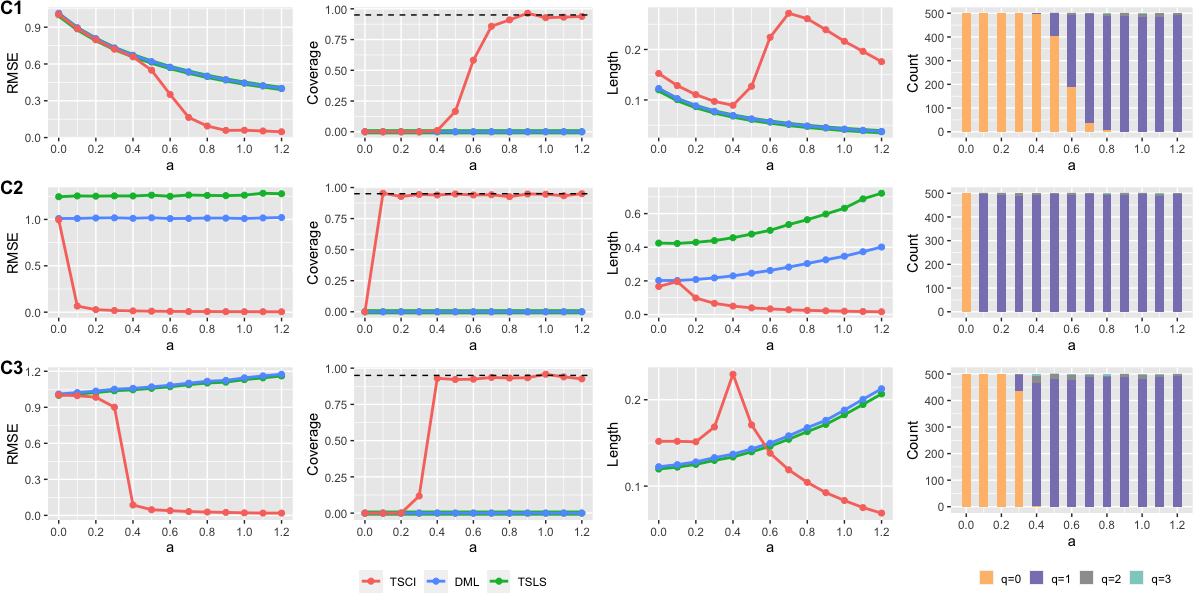
Figure 3: Comparison of TSCI, DML and TSLS in terms of RMSE, CI coverage, and length in Settings C1, C2 and C3, where $a$ controls the nonlinearity level in the treatment model. The stacked bar charts show the basis selection of TSCI, where $q=1$ corresponds to the correct selection.

We shall point out that, in Setting C2, the confidence intervals by TSCI are shorter than that of DML, even after adjusting for the linear invalid IV forms. This happens since the remaining nonlinear IV strength after adjusting for the invalidity form is even larger than the IV strength due to the linear association.

6 Real data analysis

We revisit the question on the effect of education on income (Card, 1993). We follow Card (1993) and analyze the same data set from the National Longitudinal Survey of Young Men. The outcome is the log wages (lwage), and the treatment is the years of schooling (educ). As argued in Card (1993), there are various reasons that the treatment is endogenous. For example, the unobserved confounder “ability bias” may affect both the schooling years and wages, leading to the OLS estimator having a positive bias. Following Card (1993), we use the indicator for a nearby 4-year college in 1966 (nearc4) as the IV and include the following covariates: a quadratic function of potential experience (exper and expersq), a race indicator (black), and dummy variables for residence in a standard metropolitan statistical area in 1976 (smsa) and in 1966 (smsa66), and the dummy variable for residence in the south in 1976 (south), and a full set of 8 regional dummy variables(reg1 to reg8). The data set consists of $n=3010$ observations, which is made available by the R package ivmodel (Kang et al., 2021).

We implement random forests for the treatment model and report the variable importance in Figure S4 in the supplement, where the IV nearc4 ranks the seventh in terms of variable importance, after the covariates exper,expersq, black,south,smsa,smsa66.

We allow for different IV violation forms by approximating $g(z,x)$ with various basis functions $\{\mathcal{V}_{q}\}_{q=0,1,2}$ detailed in Table 3. Particularly, since $\mathcal{V}_{0}$ does not involve the IV nearc4, $\mathcal{V}_{0}$ corresponds to the valid IV setting as assumed in the analysis of Card (1993); moreover, $\mathcal{V}_{1}$ and $\mathcal{V}_{2}$ correspond to invalid IV settings by allowing the IV nearc4 to affect the outcome directly or interactively with the baseline covariates. The main difference is that $\mathcal{V}_{1}$ includes the interaction with the six most important covariates while $\mathcal{V}_{2}$ includes all fourteen covariates.

$\mathcal{V}_{0}$	$\{\texttt{exper,expersq,black,south,smsa,smsa66,}\texttt{reg1,reg2,reg3,reg4,reg5,reg6,reg7,reg8}\}$
$\mathcal{V}_{1}$	$\mathcal{V}_{0}\cup\texttt{nearc4}\cdot\{1,\texttt{exper},\texttt{expersq},\texttt{black},\texttt{south},\texttt{smsa},\texttt{smsa66}\}$
$\mathcal{V}_{2}$	$\mathcal{V}_{0}\cup\texttt{nearc4}\cdot\{1,\texttt{exper},\texttt{expersq},\texttt{black},\texttt{south},\texttt{smsa},\texttt{smsa66},\texttt{reg1},\texttt{reg2},\texttt{reg3},\texttt{reg4},\texttt{reg5},\texttt{reg6},\texttt{reg7},\texttt{reg8}\}$

Table 3: Definitions of $\mathcal{V}_{0},\mathcal{V}_{1}$ and $\mathcal{V}_{2}$, which are used to approximate $g(\cdot)$.

We implement Algorithm 1 to choose the best from $\{\mathcal{V}_{0},\mathcal{V}_{1},\mathcal{V}_{2}\},$ and construct the TSCI estimator. Since the TSCI estimates depend on the specific sample splitting, we report 500 TSCI estimates due to 500 different splittings. On the leftmost panel of Figure 4, we compare estimates of OLS, TSLS, and TSCI, which uses $\mathcal{V}_{\widehat{q}_{c}}$ reported from Algorithm 1. The median of these 500 TSCI estimators is $0.0604$, 87.2% of these 500 estimates are smaller than the OLS estimate (0.0747), and 100% of TSCI estimates are smaller than the TSLS estimate (0.1315). In contrast to the TSLS estimator, the TSCI estimators tend to be smaller than the OLS estimator, which helps correct the positive “ability bias”.

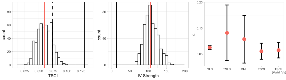
Figure 4: The leftmost panel reports the histograms of the TSCI (random forests) estimates with the comparison method, where the estimates differ due to the randomness of different 500 realized sample splittings; the solid red line corresponds to the median of the TSCI estimates, while the solid and dashed black lines correspond to the TSLS and OLS estimates, respectively. The middle panel displays the histogram of the generalized IV strength (after adjusting for $\mathcal{V}_{\widehat{q}_{c}}$) over the different 500 realized sample splittings; the solid red line denotes the median of all IV strength for TSCI while the solid black line denotes the IV strength of TSLS. The rightmost panel compares different confidence intervals (CIs) produced by OLS, TSLS, DML, and our proposed TSCI with $\mathcal{V}_{\widehat{q}_{c}}$, and TSCI assuming valid IVs. The CIs of TSCI are adjusted by the multi-splitting method due to finite samples; see Appendix A.4.

On the rightmost panel of Figure 4, we compare different confidence intervals (CIs). The TSLS CI is $(0.0238,0.2393)$, and the DML CI is $(0.0061,0.1907)$, which are both much wider than the CIs by TSCI. This wide interval results from the relatively weak IV because TSLS and DML only consider the linear association between IV and the treatment. The CI by TSCI with random forests varies with the specific sample splitting. We follow Meinshausen et al. (2009) and implement the multi-split method to adjust the finite-sample variation due to sample splitting; see Section A.4 in the supplement. The multi-split CI is (0.0294, 0.0914). The CIs based on the TSCI estimator with random forests are pushed to the lower part of the wide CI by TSLS. The CIs by our proposed TSCI in Algorithm 1 tend to shift down in comparison to the TSCI assuming valid IVs.

We shall point out that the IV strengths for the TSCI estimators, even after adjusting for the selected basis functions, are typically much larger than the TSLS (the concentration parameter is $13.33$), which is illustrated in the middle panel of Figure 4. This happens since the first-stage ML captures much more associations than the linear model in TSLS, even after adjusting for the possible IV violations captured by $\mathcal{V}_{\widehat{q}_{c}}$.

Among 500 sample splittings, the proportion of choosing $\mathcal{V}_{0},\mathcal{V}_{1},$ and $\mathcal{V}_{2}$ are $59.2\%$, $38.2\%$, and $2.6\%$, respectively, where around $41\%$ of splittings report nearc4 as invalid IVs. Importantly, $93.6\%$ out of the 500 splittings report $Q_{\text{max}}>\widehat{q}_{c}$, which represents that $\widehat{\beta}_{\mathcal{V}_{\widehat{q}_{c}}}$ is not statistically different from $\widehat{\beta}_{\mathcal{V}_{Q_{\text{max}}}}$ produced by the largest $\mathcal{V}_{Q_{\text{max}}}$. This indicates that $\mathcal{V}_{\widehat{q}_{c}}$ already provides a reasonably good approximation of $g(Z_{i},X_{i})$ in the outcome model. In Section E.1 of the supplement, we consider alternative choices of $\mathcal{V}_{2}$ and observe that the results are consistent with that reported above. In Section E.2, we further propose a falsification argument regarding Condition 1 for the data analysis.

7 Conclusion and discussion

We integrate modern ML algorithms into the framework of instrumental variable analysis. We devise a novel TSCI methodology which provides reliable causal conclusions even with a wide range of violation forms. Our proposed generalized IV strength measure helps to understand when our proposed method is reliable and supports the basis functions’ selection in approximating the violation form of possibly invalid IVs. The current methodology is focused on inference for a linear and constant treatment effect. An interesting future research direction is about inference for heterogeneous treatment effects (Athey and Imbens, 2016; Wager and Athey, 2018) but in presence of potentially invalid instruments.

Appendix A Additional Methods and Theories

A.1 Identification in random experiments with non-compliance and invalid IVs

In the following, we explain how a nonlinear treatment model helps identify the causal effect in randomized experiments with non-compliance and possibly invalid IVs. For the $i$-th subject, we use $Z_{i}\in\{0,1\}$ to denote the random treatment assignment (which serves as an instrument) and $D_{i}\in\{0,1\}$ to denote whether the subject actually takes the treatment or not. We use $X_{i}\in\{0,1\}$ to denote a binary covariate and $Y^{(z,d)}_{i}(x)$ to denote the potential outcome for a subject with the assignment $z$, the treatment value $d$, and the covariate $x$.

A primary concern is that $Z_{i}$ may be an invalid IV even if it is randomly assigned. To facilitate the discussion, we follow the discussion in imbens2014instrumental and adopt the example from mcdonald1992effects studying the effect of influenza vaccination on being hospitalized for flu-related reasons. The researchers randomly sent letters to physicians encouraging them to vaccinate their patients. In this example, $Z_{i}$ denotes the indicator for the physician receiving the encouragement letter, while $D_{i}$ stands for the patient being vaccinated or not. The outcome $Y_{i}$ denotes whether the patient is hospitalized for a flu-related reason. As pointed out in imbens2014instrumental, the physician receiving the letter may “take actions that affect the likelihood of the patient getting infected with the flu other than simply administering the flu vaccine”, indicating that $Z_{i}$ may have a direct effect on the outcome and violate the classical IV assumptions.

For a covariate $x$, we define the intention-to-treat (ITT) on the outcome as ${\rm ITT}_{Y}(x)={\mathbf{E}}(Y_{i}\mid Z_{i}=1,X_{i}=x)-{\mathbf{E}}(Y_{i}\mid Z_{i}=0,X_{i}=x)$ and the ITT on the treatment as ${\rm ITT}_{D}(x)={\mathbf{E}}(D_{i}\mid Z_{i}=1,X_{i}=x)-{\mathbf{E}}(D_{i}\mid Z_{i}=0,X_{i}=x).$ In the following proposition, we assume the constant effect and demonstrate the treatment effect identification even if the IV $Z_{i}$ directly affects the outcome (violating assumption (A2)).

Proposition 2

Suppose that (I1) ${\rm ITT}_{D}(x=1)-{\rm ITT}_{D}(x=0)\neq 0$, (I2) $Z_{i}$ is randomly assigned, (I3) $Y^{(z^{\prime},d)}_{i}(x)-Y^{(z,d)}_{i}(x)=(z^{\prime}-z)\pi$ for $x\in\{0,1\}$, and (I4) $Y^{(z,d^{\prime})}_{i}(x)-Y^{(z,d)}_{i}(x)=(d^{\prime}-d)\beta.$ Then we identify $\beta$ as $\frac{{\rm ITT}_{Y}(x=1)-{\rm ITT}_{Y}(x=0)}{{\rm ITT}_{D}(x=1)-{\rm ITT}_{D}(x=0)}.$

The proof of the above proposition is presented in Section B.1. Condition (I4) assumes a constant effect while (I1)-(I3) are relaxations of the classical IV assumptions (A1)-(A3), respectively. Particularly, the random assignment required by (I2) implies (A2) and (I2) is satisfied in randomized experiments with non-compliance. Condition (I3) allows the IV to affect the outcome directly but assumes that the IV’s direct effect does not interact with the baseline covariate $X_{i}$. When there exists a direct effect, the identification of $\beta$ relies on the Condition (I1). Condition (I1) essentially requires that the treatment assignment is interactively determined by $Z_{i}$ and $X_{i}$: a special example is given by $D_{i}={\bf 1}\left(\gamma_{0}+\gamma_{z}Z_{i}+\gamma_{x}X_{i}+\gamma Z_{i}\cdot X_{i}+\delta_{i}>0\right)$ where $\delta_{i}$ denotes a random variable independent of $Z_{i}$ and $X_{i}.$ Such identification conditions have been proposed in Shardell and Ferrucci (2016); Ten Have et al. (2007). Particularly, Shardell and Ferrucci (2016) has pointed out that ${\rm ITT}_{D}(x=1)-{\rm ITT}_{D}(x=0)$ is referred to as the compliance score and Condition (I1) requires that the compliance score changes with the covariate value $x$.

We provide now some discussions on the plausibility of Condition (I1). We still use the vaccination example from mcdonald1992effects and imagine that we may have access to the covariate $X_{i}$, an indicator for whether the patients took regular flu shots in the past few years. Patients who regularly take flu shots (with $X_{i}=1$) are more likely to follow the physician’s encouragement than those who do not (with $X_{i}=0$), indicating ${\rm ITT}_{D}(x=1)-{\rm ITT}_{D}(x=0)\neq 0$. However, regarding the concern “take actions that affect the likelihood of the patient getting infected with the flu other than simply administering the flu vaccine” imbens2014instrumental, such a direct effect of $Z_{i}$ might not interact with $X_{i}$.

A.2 Pitfalls with the naive machine learning

As the benchmarks in Section 5.2, we also include the point estimators $\widehat{\beta}_{\text{init}}$, $\widehat{\beta}_{\text{plug}},$ and $\widehat{\beta}_{\text{full}}$ together with their corresponding standard errors. We construct the 95% confidence interval as $(\widehat{\beta}-1.96*\widehat{\rm SE},\widehat{\beta}+1.96*\widehat{\rm SE}).$

RF-Init. We compute $\widehat{\beta}$ as $\widehat{\beta}_{\rm init}$ in (16) and $\widehat{\sigma}_{\epsilon}(V)=\sqrt{\|P^{\perp}_{V}[Y-D\widehat{\beta}_{\rm init}(V)]\|_{2}^{2}/(n-r)}.$ Calculate $\widehat{\rm SE}={\widehat{\sigma}_{\epsilon}\sqrt{{D}_{\mathcal{A}_{1}}^{\intercal}[\mathbf{M}(V)]^{2}{D}_{\mathcal{A}_{1}}}}/{{D}_{\mathcal{A}_{1}}^{\intercal}\mathbf{M}(V){D}_{\mathcal{A}_{1}}}.$

RF-Plug and its pitfall. A simple idea of combining TSLS with ML is to directly use $\widehat{f}_{\mathcal{A}_{1}}$ in the second stage. We may calculate such a two-stage estimator as $\widehat{\beta}_{\rm plug}(V)={{Y}_{\mathcal{A}_{1}}^{\intercal}P^{\perp}_{{V}_{\mathcal{A}_{1}}}\widehat{f}_{\mathcal{A}_{1}}}/{\widehat{f}_{\mathcal{A}_{1}}^{\intercal}P^{\perp}_{{V}_{\mathcal{A}_{1}}}\widehat{f}_{\mathcal{A}_{1}}},$ where the second-stage regression is implemented by regressing $Y_{\mathcal{A}_{1}}$ on $\widehat{f}_{\mathcal{A}_{1}}=\Omega D_{\mathcal{A}_{1}}$ and $V_{\mathcal{A}_{1}}$. We compute the standard error $\widehat{\rm SE}=\sqrt{\frac{\|P^{\perp}_{V}(Y-\widehat{\beta}_{\rm plug}(V)D)\|_{2}^{2}}{|\mathcal{A}_{1}|\cdot{\widehat{D}_{\mathcal{A}_{1}}^{\intercal}P^{\perp}_{{V}_{\mathcal{A}_{1}}}}}}.$ angrist2009mostly[Sec.4.6.1] criticized such use of the nonlinear first-stage model under the name of “forbidden regression” and chen2020mostly pointed out that $\widehat{\beta}_{\rm plug}(V)$ is biased since $\Omega$ in (12) is not a projection matrix for random forests.

RF-Full and its pitfall. Sample splitting is essential for removing the endogeneity of the ML-predicted values. Without sample splitting, the ML predicted value for the treatment can be close to the treatment (due to overfitting) and hence highly correlated with unmeasured confounders, leading to a TSCI estimator suffering from a significant bias. In the following, we take the non-split Random Forests as an example. Similarly to $\Omega$ defined in (12), we define the transformation matrix $\Omega^{\rm full}$ for random forests constructed with the full data. As a modification of (16), we consider the corresponding TSCI estimator,

$$\widehat{\beta}_{\rm full}(V)={Y^{\intercal}\mathbf{M}^{\rm full}(V){D}}/{{D}^{\intercal}\mathbf{M}^{\rm full}(V){D}}\quad\text{with}\quad\mathbf{M}^{\rm full}_{\rm RF}(V)=(\Omega^{\rm full})^{\intercal}P^{\perp}_{\widetilde{V}}\Omega^{\rm full},$$ (38)

where $\widetilde{V}=\Omega^{\rm full}V$. We calculate its standard error as

$$\widehat{\rm SE}=\frac{\widehat{\sigma}_{\rm full}(V)\sqrt{{{D}^{\intercal}[\mathbf{M}^{\rm full}(V)]^{2}{D}}}}{{D}^{\intercal}\mathbf{M}^{\rm full}(V){D}}\quad\text{with}\quad\widehat{\sigma}_{\rm full}(V)=\sqrt{\|P^{\perp}_{V}(Y-\widehat{\beta}_{\rm RF}^{\rm full}(V)D)\|_{2}^{2}/{n}}.$$

The simulation results in Section 5 show that the estimator $\widehat{\beta}_{\rm full}(V)$ in (38) suffers from a large bias and the resulting confidence interval does not achieve the desired coverage.

A.3 Choice of $\widehat{\rho}$ in (27)

In the following, we present the choice of $\widehat{\rho}=\widehat{\rho}(\alpha_{0})>0$ used in (27) by the wild bootstrap. For $1\leq i\leq n_{1},$ we compute $\widetilde{\epsilon}_{i}=[\widehat{\epsilon}(V_{Q_{\max}})]_{i}-\bar{\mu}_{\epsilon}$ where $\widehat{\epsilon}(V_{Q_{\max}})$ is defined in (21) with $V=V_{Q_{\max}}$ and $\bar{\mu}_{\epsilon}=\frac{1}{n_{1}}\sum_{i=1}^{n_{1}}[\widehat{\epsilon}(V_{Q_{\max}})]_{i}$. We generate $\epsilon^{[l]}_{i}=U^{[l]}_{i}\cdot\widetilde{\epsilon}_{i}$ for $1\leq i\leq n_{1}$ and $1\leq l\leq L,$ where $\{U^{[l]}_{i}\}_{1\leq i\leq n_{1}}$ are i.i.d. standard normal random variables. We define

$$T^{[l]}=\max_{0\leq q<q^{\prime}\leq Q_{\max}}\frac{1}{{\sqrt{\widehat{H}(V_{q},V_{q^{\prime}})}}}\left[\frac{f_{\mathcal{A}_{1}}^{\intercal}\mathbf{M}(V_{q^{\prime}})\epsilon^{[l]}}{{f}_{\mathcal{A}_{1}}^{\intercal}\mathbf{M}(V_{q^{\prime}})f_{\mathcal{A}_{1}}}-\frac{f_{\mathcal{A}_{1}}^{\intercal}\mathbf{M}(V_{q})\epsilon^{[l]}}{f_{\mathcal{A}_{1}}^{\intercal}\mathbf{M}(V_{q})f_{\mathcal{A}_{1}}}\right]\;\text{for}\;1\leq l\leq L.$$

We set $\widehat{\rho}=\widehat{\rho}(\alpha_{0})$ to be the upper $\alpha_{0}$ empirical quantile of $\{|T^{[l]}|\}_{1\leq l\leq L}$, that is,

$$\widehat{\rho}(\alpha_{0})=\min\left\{\rho\in\mathbb{R}:\frac{1}{L}\sum_{l=1}^{L}{\bf 1}\left(|{T^{[l]}}|\leq\rho\right)\geq 1-\alpha_{0}\right\},$$ (39)

where $\alpha_{0}$ is set as $0.025$ by default.

A.4 Finite-sample adjustment of uncertainty from data splitting

Even though our asymptotic theory in Section 4 is valid for any random sample splitting, the constructed point estimators and confidence intervals do vary with different sample splittings in finite samples. This randomness due to sample splittings has been also observed in double machine learning chernozhukov2018double and multi-splitting meinshausen2009p. Following chernozhukov2018double and meinshausen2009p, we introduce a confidence interval which aggregates multiple confidence intervals due to different splittings. Consider $S$ random splittings and for the $s$-th splitting, we use $\widehat{\beta}^{s}$ and $\widehat{\rm SE}^{s}$ to denote the corresponding TSCI point and standard error estimators, respectively. Following Section 3.4 of chernozhukov2018double, we introduce the median estimator $\widehat{\beta}^{\rm med}={\rm median}\{\widehat{\beta}^{s}\}_{1\leq s\leq S}$ together with $\widehat{\rm SE}^{\rm med}={\rm median}\left\{\sqrt{[\widehat{\rm SE}^{s}]^{2}+(\widehat{\beta}^{s}-\widehat{\beta}^{\rm med})^{2}}\right\}_{1\leq s\leq S},$ and construct the median confidence interval as $(\widehat{\beta}^{\rm med}-z_{\alpha/2}\widehat{\rm SE}^{\rm med},\widehat{\beta}^{\rm med}+z_{\alpha/2}\widehat{\rm SE}^{\rm med}).$ Alternatively, following meinshausen2009p, we construct the p values $p^{s}(\beta_{0})=2(1-\Phi(|\widehat{\beta}^{s}-\beta_{0}|/\widehat{\rm SE}^{s}))$ for $\beta_{0}\in\mathbb{R}$ and $1\leq s\leq S,$ where $\Phi$ is the CDF of the standard normal. We define the multi-splitting confidence interval as $\{\beta_{0}\in\mathbb{R}:2\cdot{\rm median}\{p^{s}(\beta_{0})\}_{s=1}^{S}\geq\alpha\}.$ See equation (2.2) of meinshausen2009p.

A.5 Choices of Violation Basis Functions for Multiple IVs

When there are multiple IVs, there are more choices to specify the violation form, and $\{\mathcal{V}_{q}\}_{1\leq q\leq Q}$ are not necessarily nested. For example, when we have two IVs $z_{1}$ and $z_{2}$, we may set $\mathcal{V}_{q_{1},q_{2}}=\{1,z_{1},\cdots,z_{1}^{q_{1}},z_{2},\cdots,z_{2}^{q_{2}}\},$ and then $\{\mathcal{V}_{q_{1},q_{2}}\}_{0\leq q_{1},q_{2}\leq Q}$ are not nested. However, even in such a case, our proposed selection method is still applicable. Specifically, for any $0\leq q_{1},q_{2}\leq Q$, we compare the estimator generated by $\mathcal{V}_{q_{1},q_{2}}$ to that by $\mathcal{V}_{q^{\prime}_{1},q^{\prime}_{2}}$ with $q^{\prime}_{1}\geq q_{1}$ and $q^{\prime}_{2}\geq q_{2}.$

A.6 TSCI with boosting

In the following, we demonstrate how to express the $L_{2}$ boosting estimator buhlmann2007boosting,buhlmann2006sparse in the form of (12). The boosting methods aggregate a sequence of base procedures $\{\widehat{g}^{[m]}(\cdot)\}_{m\geq 1}.$ For $m\geq 1,$ we construct the base procedure $\widehat{g}^{[m]}$ using the data in $\mathcal{A}_{2}$ and compute the estimated values given by the $m$-th base procedure $\widehat{g}^{[m]}_{\mathcal{A}_{1}}=\left(\widehat{g}^{[m]}(X_{1},Z_{1}),\cdots,\widehat{g}^{[m]}(X_{n_{1}},Z_{n_{1}})\right)^{\intercal}$. With $\widehat{f}^{[0]}_{\mathcal{A}_{1}}=0$ and $0<\nu\leq 1$ as the step-length factor (the default being $\nu=0.1$), we conduct the sequential updates,

$$\widehat{f}^{[m]}_{\mathcal{A}_{1}}=\widehat{f}^{[m-1]}_{\mathcal{A}_{1}}+\nu\widehat{g}^{[m]}_{\mathcal{A}_{1}}\quad\text{with}\quad\widehat{g}^{[m]}_{\mathcal{A}_{1}}=\mathcal{H}^{[m]}(D_{\mathcal{A}_{1}}-\widehat{f}^{[m-1]}_{\mathcal{A}_{1}})\quad\text{for}\quad m\geq 1,$$

where $\mathcal{H}^{[m]}\in\mathbb{R}^{n_{1}\times n_{1}}$ is a hat matrix determined by the base procedures.

With the stopping time $m_{\rm stop}$, the $L_{2}$ boosting estimator is $\widehat{f}^{\rm boo}=\widehat{f}^{[m_{\rm stop}]}.$ We now compute the transformation matrix $\Omega$. Set $\Omega^{[0]}=0$ and for $m\geq 1,$ we define

$$\widehat{f}^{[m]}_{\mathcal{A}_{1}}=\Omega^{[m]}D_{\mathcal{A}_{1}}\quad\text{with}\quad\Omega^{[m]}=\nu\mathcal{H}^{[m]}+({\rm I}-\nu\mathcal{H}^{[m]})\Omega^{[m-1]}.$$ (40)

Define $\Omega^{\rm boo}=\Omega^{[m_{\rm stop}]}$ and write $\widehat{f}^{\rm boo}=\Omega^{\rm boo}D_{\mathcal{A}_{1}},$ which is the desired form in (12).

In the following, we give two examples of the construction of the base procedures and provide the detailed expression for $\mathcal{H}^{[m]}$ used in (40). We write $C_{i}=(X_{i}^{\intercal},Z_{i}^{\intercal})^{\intercal}\in\mathbb{R}^{p}$ and define the matrix $C\in\mathbb{R}^{n\times p}$ with its $i$-th row as $C_{i}^{\intercal}.$ An important step of building the base procedures $\{\widehat{g}^{[m]}(Z_{i},X_{i})\}_{m\geq 1}$ is to conduct the variable selection. That is, each base procedure is only constructed based on a subset of covariates $C_{i}=(X_{i}^{\intercal},Z_{i}^{\intercal})\in\mathbb{R}^{p}.$

Pairwise regression.

In Algorithm 2, we describe the construction of $\Omega^{\rm boo}$ with the pairwise regression and the pairwise thin plate as the base procedure. For both base procedures, we need to specify how to construct the basis functions in steps 3 and 8. For the pairwise regression, we set the first element of $C_{i}$ as $1$ and define $S^{j,l}_{i}=C_{ij}C_{il}$ for $1\leq i\leq n.$ Then for step 3, we define $\mathcal{P}^{j,l}$ as the projection matrix to the vector $S^{j,l}_{\mathcal{A}_{2}};$ for step 8, we define $\mathcal{H}^{[m]}=(S^{\widehat{j}_{m},\widehat{l}_{m}}_{\mathcal{A}_{1}})^{\intercal}/{\|S^{\widehat{j}_{m},\widehat{l}_{m}}_{\mathcal{A}_{1}}\|_{2}^{2}}.$

For the pairwise thin plate, we follow chapter 7 of green1993nonparametric to construct the projection matrix. For $1\leq j<l\leq p,$ we define the matrix $T^{j,l}=\begin{pmatrix}1&1&\cdots&1\\ X_{1,j}&X_{2,j}&\cdots&X_{n,j}\\ X_{1,l}&X_{2,l}&\cdots&X_{n,l}\end{pmatrix}.$ For $1\leq s\leq n,$ define $E^{j,l}_{s,s}=0$; for $1\leq s\neq t\leq n,$ define

$$E^{j,l}_{s,t}=\frac{1}{16\pi}\left\|(X_{s,(j,l)}-X_{t,(j,l)}\right\|_{2}^{2}\log(\left\|(X_{s,(j,l)}-X_{t,(j,l)}\right\|_{2}^{2}).$$

Then we define $\bar{\mathcal{P}}^{j,l}=\begin{pmatrix}E^{j,l}_{\mathcal{A}_{2},\mathcal{A}_{2}}&(T^{j,l}_{\cdot,\mathcal{A}_{2}})^{\intercal}\end{pmatrix}\begin{pmatrix}E^{j,l}_{\mathcal{A}_{2},\mathcal{A}_{2}}&(T^{j,l}_{\cdot,\mathcal{A}_{2}})^{\intercal}\\ T^{j,l}_{\cdot,\mathcal{A}_{2}}&0\end{pmatrix}^{-1}\in\mathbb{R}^{n_{2}\times(n_{2}+3)}$. In step 3, compute $\mathcal{P}^{j,l}\in\mathbb{R}^{n_{2}\times n_{2}}$ as the first $n_{2}$ columns of $\bar{\mathcal{P}}^{j,l}.$ For step 8, we compute

$$\bar{\mathcal{H}}^{j,l}=\begin{pmatrix}E^{j,l}_{\mathcal{A}_{1},\mathcal{A}_{1}}&(T^{j,l}_{\cdot,\mathcal{A}_{1}})^{\intercal}\end{pmatrix}\begin{pmatrix}E^{j,l}_{\mathcal{A}_{1},\mathcal{A}_{1}}&(T^{j,l}_{\cdot,\mathcal{A}_{1}})^{\intercal}\\ T^{j,l}_{\cdot,\mathcal{A}_{1}}&0\end{pmatrix}^{-1}\in\mathbb{R}^{n_{1}\times(n_{1}+3)},$$

and set $\mathcal{H}^{[m]}\in\mathbb{R}^{n_{1}\times n_{1}}$ as the first $n_{1}$ columns of $\bar{\mathcal{H}}^{\widehat{j}_{m},\widehat{l}_{m}}.$

Algorithm 2 Construction of $\Omega$ in Boosting with non-parametric pairwise regression

Input: Data $C\in\mathbb{R}^{n\times p},D\in\mathbb{R}^{n}$; the step-length factor $0<\nu\leq 1$; the stoping time $m_{\rm stop}.$

Output: $\Omega^{\rm boo}$

1:Randomly split the data into disjoint subsets $\mathcal{A}_{1},\mathcal{A}_{2}$ with $n_{1}=\lfloor\frac{2n}{3}\rfloor$ and $|\mathcal{A}_{2}|=n-n_{1}$;

2:Set $m=0,$ $\widehat{f}^{[0]}_{\mathcal{A}_{2}}=0,$ and $\Omega^{[0]}=0.$

3:For $1\leq j,l\leq p$, compute $\mathcal{P}^{j,l}$ as the projection matrix to a set of basis functions generated by $C_{\mathcal{A}_{2},j}$ and $C_{\mathcal{A}_{2},l}.$

4:for $1\leq m\leq m_{\rm stop}$ do

5:     Compute the adjusted outcome $U^{[m]}_{\mathcal{A}_{2}}=D_{\mathcal{A}_{2}}-\widehat{f}^{[m-1]}_{\mathcal{A}_{2}}$

6:     Implement the following base procedure on $\{C_{i},U^{[m]}_{i}\}_{i\in\mathcal{A}_{2}}$

$$(\widehat{j}_{m},\widehat{l}_{m})=\operatorname*{arg\,min}_{1\leq j,l\leq p}\left\|U^{[m]}_{\mathcal{A}_{2}}-\mathcal{P}^{j,l}U^{[m]}_{\mathcal{A}_{2}}\right\|^{2}.$$

7:     Update $\widehat{f}^{[m]}_{\mathcal{A}_{2}}=\widehat{f}^{[m-1]}_{\mathcal{A}_{2}}+\nu\mathcal{P}^{\widehat{j}_{m},\widehat{l}_{m}}\left(D_{\mathcal{A}_{2}}-\widehat{f}^{[m-1]}_{\mathcal{A}_{2}}\right)$

8:     Construct $\mathcal{H}^{[m]}$ in the same way as $\mathcal{P}^{\widehat{j}_{m},\widehat{l}_{m}}$ but with the data in $\mathcal{A}_{1}.$

9:     Compute $\Omega^{[m]}=\nu\mathcal{H}^{[m]}+({\rm I}-\nu\mathcal{H}^{[m]})\Omega^{[m-1]}$

10:end for

11:Return $\Omega^{\rm boo}$

Decision tree.

In Algorithm 3, we describe the construction of $\Omega^{\rm boo}$ with the decision tree as the base procedure.

Algorithm 3 Construction of $\Omega$ in Boosting with Decision tree

Input: Data $C\in\mathbb{R}^{n\times p},D\in\mathbb{R}^{n}$; the step-length factor $0<\nu\leq 1$; the stoping time $m_{\rm stop}.$

Output: $\Omega^{\rm boo}$

1:Randomly split the data into disjoint subsets $\mathcal{A}_{1},\mathcal{A}_{2}$ with $n_{1}=\lfloor\frac{2n}{3}\rfloor$ and $|\mathcal{A}_{2}|=n-n_{1}$;

2:Set $m=0,$ $\widehat{f}^{[0]}_{\mathcal{A}_{2}}=0,$ and $\Omega^{[0]}=0.$

3:for $1\leq m\leq m_{\rm stop}$ do

4:     Compute the adjusted outcome $U^{[m]}_{\mathcal{A}_{2}}=D_{\mathcal{A}_{2}}-\widehat{f}^{[m-1]}_{\mathcal{A}_{2}}$

5:     Run the decision tree on $\{C_{i},U^{[m]}_{i}\}_{i\in\mathcal{A}_{2}}$ and partition $\mathbb{R}^{p}$ as leaves $\{\mathcal{R}^{[m]}_{1},\cdots,\mathcal{R}^{[m]}_{L}\};$

6:     For any $j\in\mathcal{A}_{2},$ we identify the leaf $\mathcal{R}^{[m]}_{l(C_{j})}$ containing $C_{j}$ and compute

$$\mathcal{P}^{[m]}_{j,t}=\frac{{\bf{1}}\left[C_{t}\in\mathcal{R}^{[m]}_{l(C_{j})}\right]}{\sum_{k\in\mathcal{A}_{2}}{\bf{1}}\left[C_{k}\in\mathcal{R}^{[m]}_{l(C_{j})}\right]}\quad\text{for}\quad t\in\mathcal{A}_{2}$$

7:     Compute the matrix $(\mathcal{P}^{[m]}_{j,t})_{j,t\in\mathcal{A}_{2}}$ and update

$$\widehat{f}^{[m]}_{\mathcal{A}_{2}}=\widehat{f}^{[m-1]}_{\mathcal{A}_{2}}+\nu\mathcal{P}^{[m]}\left(D_{\mathcal{A}_{2}}-\widehat{f}^{[m-1]}_{\mathcal{A}_{2}}\right)$$

8:     Construct the matrix $(\mathcal{H}^{[m]}_{j,t})_{j,t\in{\mathcal{A}_{1}}}$ as $\mathcal{H}^{[m]}_{j,t}=\frac{{\bf{1}}\left[C_{t}\in\mathcal{R}^{[m]}_{l(C_{j})}\right]}{{\sum_{k\in\mathcal{A}_{1}}}{\bf{1}}\left[C_{k}\in\mathcal{R}^{[m]}_{l(C_{j})}\right]}.$

9:     Compute $\Omega^{[m]}=\nu\mathcal{H}^{[m]}+({\rm I}-\nu\mathcal{H}^{[m]})\Omega^{[m-1]}$

10:end for

11:Return $\Omega^{\rm boo}$

A.7 TSCI with deep neural network

In the following, we demonstrate how to calculate $\Omega$ for a deep neural network james2013introduction. We define the first hidden layer as $H^{(1)}_{i,k}=\sigma\left(\omega^{(1)}_{k,0}+\sum_{l=1}^{p_{\rm z}}\omega^{(1)}_{k,l}Z_{il}+\sum_{l=1}^{p_{\rm x}}\omega^{(1)}_{k,l+p_{\rm z}}X_{i,l}\right)$ for $1\leq k\leq K_{1},$ where $\sigma(\cdot)$ is the activation function and $\{\omega^{(1)}_{k,l}\}_{1\leq k\leq K_{1},1\leq l\leq p_{x}+p_{z}}$ are parameters. For $m\geq 2$, we define the $m$-th hidden layer as $H^{(m)}_{i,k}=\sigma\left(\omega^{(m)}_{k,0}+\sum_{l=1}^{K_{m-1}}\omega^{(m)}_{k,l}H^{(m-1)}_{i,l}\right)$ for $1\leq k\leq K_{m},$ where $\{\omega^{(m)}_{k,l}\}_{1\leq k\leq K_{m},1\leq l\leq K_{m-1}}$ are unknown parameters. For given $M\geq 1,$ we estimate the unknown parameters based on the data $\{X_{i},Z_{i},D_{i}\}_{i\in\mathcal{A}_{2}}$,

$$\left\{\widehat{\beta},\{\widehat{\omega}^{(m)}\}_{1\leq m\leq M}\right\}\coloneqq\operatorname*{arg\,min}_{\{\beta_{k}\}_{0\leq k\leq K_{M}},\{\omega^{(m)}\}_{1\leq m\leq M}}\sum_{i\in\mathcal{A}_{2}}\left(Y_{i}-\beta_{0}-\sum_{k=1}^{K_{M}}\beta_{k}H^{(M)}_{i,k}\right)^{2}.$$

With $\{\widehat{\omega}^{(m)}\}_{1\leq m\leq M},$ for $1\leq m\leq M$ and $1\leq i\leq n_{1}$, we define

$$\widehat{H}^{(m)}_{i,k}=\sigma\left(\widehat{\omega}^{(m)}_{k0}+\sum_{l=1}^{K_{m-1}}\widehat{\omega}^{(m)}_{kl}H^{(m-1)}_{i,l}\right)\quad\text{for}\quad 1\leq k\leq K_{m}$$

with $\widehat{H}^{(1)}_{i,k}=\sigma\left(\widehat{\omega}^{(1)}_{k0}+\sum_{l=1}^{p_{\rm z}}\widehat{\omega}^{(1)}_{kl}Z_{il}+\sum_{l=1}^{p_{\rm x}}\widehat{\omega}^{(1)}_{k,l+p_{\rm z}}X_{il}\right)$ for $1\leq k\leq K_{1}.$ We use $\Omega^{\rm DNN}=\widehat{H}^{(M)}\left([\widehat{H}^{(M)}]^{\intercal}\widehat{H}^{(M)}\right)^{-1}[\widehat{H}^{(M)}]^{\intercal}$ to denote the projection to the column space of the matrix $\widehat{H}^{(M)}$ and express the deep neural network estimator as $\Omega^{\rm DNN}D_{\mathcal{A}_{1}}.$ With $\widehat{V}_{\mathcal{A}_{1}}=\Omega^{\rm DNN}V_{\mathcal{A}_{1}},$ we define $\mathbf{M}_{\rm DNN}(V)=\left[\Omega^{\rm DNN}\right]^{\intercal}P^{\perp}_{\widehat{V}_{\mathcal{A}_{1}}}\Omega^{\rm DNN},$ which is shown to be an orthogonal projection matrix in Lemma 1 in the supplement.

A.8 TSCI with B-spline

As a simplification, we consider the additive model ${\mathbf{E}}(D_{i}\mid Z_{i},X_{i})=\gamma_{1}(Z_{i})+\gamma_{2}(X_{i}),$ and assume that $\gamma_{1}(\cdot)$ can be well approximated by a set of B-spline functions $\{b_{1}(\cdot),\cdots,b_{M}(\cdot)\}.$ In practice, the number $M$ can be chosen by cross-validation. We define the matrix $B\in\mathbb{R}^{n\times M}$ with its $i$-th row $B_{i}=\left(b_{1}(Z_{i}),\cdots,b_{M}(Z_{i})\right)^{\intercal}.$ Without loss of generality, we approximate $\gamma_{2}(X_{i})$ by $W_{i}\in\mathbb{R}^{p_{w}}$, which is generated by the same set of basis functions for $\phi(X_{i})$. Define $\Omega^{\rm ba}=P_{BW}\in\mathbb{R}^{n\times n}$ as the projection matrix to the space spanned by the columns of $B\in\mathbb{R}^{n\times k}$ and $W\in\mathbb{R}^{n\times p_{w}}$. We write the first-stage estimator as $\Omega^{\rm ba}D$ and compute $\mathbf{M}_{\rm ba}(V)=\left[\Omega^{\rm ba}\right]^{\intercal}P^{\perp}_{\widehat{V},{W}}\Omega^{\rm ba}$ with $\widehat{V}=\Omega^{\rm ba}V.$ The transformation matrix $\mathbf{M}_{\rm ba}(V)$ is a projection matrix with $M-{\rm rank}(V)\leq{\rm rank}\left[\mathbf{M}_{\rm ba}(V)\right]\leq M.$ When the basis number $M$ is small and the degree of freedom $M+p_{w}$ is much smaller than $n$, sample splitting is not even needed for if the B-spline is used for fitting the treatment model, which is different from the general machine learning algorithms.

A.9 Properties of $\mathbf{M}(V)$

The following lemma is about the property of the transformation matrix $\mathbf{M}(V)$, whose proof can be found in Section C.4. Recall that

$$\mathbf{M}_{\rm RF}({V})=\Omega^{\intercal}P^{\perp}_{\widehat{V}_{\mathcal{A}_{1}}}\Omega\quad\text{with}\quad\Omega_{ij}=\omega_{j}(Z_{i},X_{i}),$$

where $\omega_{j}(z,x)$ is defined in (14).

Lemma 1

The transformation matrix $\mathbf{M}_{\rm RF}({V})$ satisfies

$$\lambda_{\max}(\mathbf{M}_{\rm RF}({V}))\leq 1\quad\text{and}\quad b^{\intercal}[\mathbf{M}_{\rm RF}({V})]^{2}b\leq b^{\intercal}\mathbf{M}_{\rm RF}({V})b\quad\text{for any}\quad b\in\mathbb{R}^{n_{1}}.$$ (41)

As a consequence, we establish ${\rm Tr}\left([\mathbf{M}_{\rm RF}({V})]^{2}\right)\leq{\rm Tr}[\mathbf{M}(V)].$ The transformation matrixs $\mathbf{M}_{\rm ba}(V)$ and $\mathbf{M}_{\rm DNN}({V})$ are orthogonal projection matrices with

$$[\mathbf{M}_{\rm ba}(V)]^{2}=\mathbf{M}_{\rm ba}(V)\quad\text{and}\quad[\mathbf{M}_{\rm DNN}({V})]^{2}=\mathbf{M}_{\rm DNN}({V}).$$ (42)

The transformation matrix $\mathbf{M}_{\rm boo}({V})$ satisfies

$$\lambda_{\max}(\mathbf{M}_{\rm boo}({V}))\leq\|\Omega^{\rm boo}\|_{2}^{2},\quad\text{and}\quad b^{\intercal}[\mathbf{M}_{\rm boo}({V})]^{2}b\leq\|\Omega^{\rm boo}\|_{2}^{2}\cdot b^{\intercal}\mathbf{M}_{\rm boo}({V})b,$$ (43)

for any $b\in\mathbb{R}^{n_{1}}.$ As a consequence, we establish ${\rm Tr}\left([\mathbf{M}_{\rm boo}({V})]^{2}\right)\leq\|\Omega^{\rm boo}\|_{2}^{2}\cdot{\rm Tr}[\mathbf{M}(V)].$

A.10 Homoscadastic correlation

In the following, we discuss the simplified method and theory in the homoscadastic correlation setting, that is, ${\rm Cov}(\epsilon_{i},\delta_{i}\mid Z_{i},X_{i})={\rm Cov}(\epsilon_{i},\delta_{i})$. With this extra assumption, we present the following bias-corrected estimator as an alternative to the estimator defined in (19),

$$\widetilde{\beta}_{\rm RF}(V)=\widehat{\beta}_{\rm init}(V)-\frac{\widehat{\rm Cov}(\delta_{i},\epsilon_{i})\cdot{\rm Tr}[\mathbf{M}(V)]}{{D}_{\mathcal{A}_{1}}^{\intercal}\mathbf{M}(V){D}_{\mathcal{A}_{1}}},$$

where $\widehat{\beta}_{\rm init}(V)$ is defined in (16) and the estimator of ${\rm Cov}(\delta_{i},\epsilon_{i})$ is defined as,

$$\widehat{\rm Cov}(\delta_{i},\epsilon_{i})=\frac{1}{n_{1}-r}(D_{\mathcal{A}_{1}}-\widehat{f}_{\mathcal{A}_{1}})^{\intercal}P^{\perp}_{V_{\mathcal{A}_{1}}}[Y_{\mathcal{A}_{1}}-D_{\mathcal{A}_{1}}\widehat{\beta}_{\rm init}(V)],$$

with $r$ denoting the rank of the matrix $(V,W)$. The correction in constructing $\widetilde{\beta}_{\rm RF}(V)$ implicitly requires ${\rm Cov}(\epsilon_{i},\delta_{i}\mid Z_{i},X_{i})={\rm Cov}(\epsilon_{i},\delta_{i}),$ which might limit practical applications.

We present a simplified version of Theorem 6 by assuming homoscadastic correlation. We shall only present the results for the TSCI with random forests but the extension to the general machine learning methods is straightforward.

Theorem 4

Consider the model (3) and (4) with ${\rm Cov}(\epsilon_{i},\delta_{i}\mid Z_{i},X_{i})={\rm Cov}(\epsilon_{i},\delta_{i})$. Suppose that Conditions (R1) and (R2) hold, then

$$\left|\widehat{\rm Cov}(\delta_{i},\epsilon_{i})-{\rm Cov}(\delta_{i},\epsilon_{i})\right|\leq\eta^{0}_{n}(V)\leq\eta_{n}(V),$$ (44)

where $\eta_{n}(V)$ is defined in (30) and

$$\eta^{0}_{n}(V)=\frac{\|f_{\mathcal{A}_{1}}-\widehat{f}_{\mathcal{A}_{1}}\|_{2}}{\sqrt{n}}+\sqrt{\frac{\log n}{n}}+\left(|\beta-\widehat{\beta}_{\rm init}(V)|+\frac{\|R(V)\|_{2}}{\sqrt{n}}\right)\left(1+\frac{\|f_{\mathcal{A}_{1}}-\widehat{f}_{\mathcal{A}_{1}}\|_{2}}{\sqrt{n}}\right).$$ (45)

Furthermore, if we assume (31) holds, then $\widetilde{\beta}_{\rm RF}(V)$ satisfies

$$\frac{1}{{\rm SE}(V)}\left(\widetilde{\beta}_{\rm RF}(V)-\beta\right)={\mathcal{G}}(V)+\mathcal{E}(V),$$ (46)

where ${\rm SE}(V)$ is defined in (59), ${\mathcal{G}}(V)\overset{d}{\to}N(0,1)$ and there exist positive constants $C>0$ and $t_{0}>0$ such that

$$\liminf_{n\rightarrow\infty}\mathbb{P}\left(\left|\mathcal{E}(V)\right|\leq C\frac{\eta^{0}_{n}(V)\cdot{\rm Tr}[\mathbf{M}(V)]+\|R(V)\|_{2}+t_{0}\sqrt{{\rm Tr}([\mathbf{M}_{\rm RF}({V})]^{2})}}{\sqrt{{f}_{\mathcal{A}_{1}}[\mathbf{M}(V)]^{2}{f}_{\mathcal{A}_{1}}}}\right)\geq 1-\exp(-t_{0}^{2}),$$ (47)

with $\eta^{0}_{n}(V)$ defined in (45).

As a remark, if $\|R(V)\|_{2}/\sqrt{n}\rightarrow 0$, $\widehat{\beta}_{\rm init}(V)\overset{p}{\to}\beta$, and ${\|f_{\mathcal{A}_{1}}-\widehat{f}_{\mathcal{A}_{1}}\|_{2}}/{\sqrt{n}}\rightarrow 0,$ then we have $\eta^{0}_{n}(V)\rightarrow 0.$

A.11 Consistency of variance estimators

The following lemma controls the variance consistency, whose proof can be found in Section C.5.

Lemma 2

Suppose that Conditions (R1) and (R2) hold and $\kappa_{n}(V)^{2}+\sqrt{\log n}\kappa_{n}(V)\overset{p}{\to}0,$ with $\kappa_{n}(V)=\sqrt{\log n}\left(\|R(V)\|_{\infty}+|\beta-\widehat{\beta}_{\rm init}(V)|+{\log n}/{\sqrt{n}}\right).$ If

$$\frac{{\sum_{i=1}^{n_{1}}\sigma^{2}_{i}[\mathbf{M}(V){D}_{\mathcal{A}_{1}}]_{i}^{2}}}{{\sum_{i=1}^{n_{1}}\sigma^{2}_{i}[\mathbf{M}(V){f}_{\mathcal{A}_{1}}]_{i}^{2}}}\overset{p}{\to}1,\quad\text{and}\quad\frac{\max_{1\leq i\leq n_{1}}[\mathbf{M}(V){D}_{\mathcal{A}_{1}}]_{i}^{2}}{{{\sum_{i=1}^{n_{1}}[\mathbf{M}(V){D}_{\mathcal{A}_{1}}]_{i}^{2}}}}\overset{p}{\to}0,$$

then we have ${\widehat{\rm SE}(V)}/{{\rm SE}(V)}\overset{p}{\to}1.$

A.12 Size and Power of $\mathcal{C}(V_{q},V_{q^{\prime}})$

The limiting distribution in Theorem 2 implies the size and power of the comparison test $\mathcal{C}(V_{q},V_{q^{\prime}})$ in (26), stated in the following theorem.

Theorem 5

Suppose that the Conditions of Theorem 2 hold, $\widehat{H}(V_{q},V_{q^{\prime}})/H(V_{q},V_{q^{\prime}})\overset{p}{\to}1$, and $\mathcal{L}_{n}(V_{q},V_{q^{\prime}})$ defined in (35) satisfies $\mathcal{L}_{n}(V_{q},V_{q^{\prime}})\overset{p}{\to}\mathcal{L}^{*}(V_{q},V_{q^{\prime}})$ for $\mathcal{L}^{*}(V_{q},V_{q^{\prime}})\in\mathbb{R}\cup\{-\infty,\infty\},$ then the test $\mathcal{C}(V_{q},V_{q^{\prime}})$ in (26) with corresponding $\alpha_{0}$ satisfies,

$$\lim_{n\rightarrow\infty}\mathbf{P}\left(\mathcal{C}(V_{q},V_{q^{\prime}})=1\right)=1-\Phi\left(z_{\alpha_{0}}-\mathcal{L}^{*}(V_{q},V_{q^{\prime}})\right)+\Phi\left(-z_{\alpha_{0}}-\mathcal{L}^{*}(V_{q},V_{q^{\prime}})\right).$$ (48)

With $\left|\mathcal{L}^{*}(V_{q},V_{q^{\prime}})\right|=0$, then we have $\lim_{n\rightarrow\infty}\mathbf{P}\left(\mathcal{C}(V_{q},V_{q^{\prime}})=1\right)=2\alpha_{0}.$ With $\left|\mathcal{L}^{*}(V_{q},V_{q^{\prime}})\right|=\infty$, then we have $\lim_{n\rightarrow\infty}\mathbf{P}\left(\mathcal{C}(V_{q},V_{q^{\prime}})=1\right)=1.$

Appendix B Proofs

We establish Proposition 2 in Section B.1. In Section B.2, we establish Proposition 1. In Section B.3, we establish Theorems 6 and 1. We prove Theorems 2 and 5 in Section B.4. We establish Theorem 3 in Section B.5 and prove Theorem 4 in Section B.6.

We define the conditional covariance matrices $\Lambda,\Sigma^{\delta},\Sigma^{\epsilon}\in\mathbb{R}^{n_{1}\times n_{1}}$ as $\Lambda={\mathbf{E}}({\delta}_{\mathcal{A}_{1}}{\epsilon}_{\mathcal{A}_{1}}^{\intercal}\mid X_{\mathcal{A}_{1}},Z_{\mathcal{A}_{1}}),$ $\Sigma^{\delta}={\mathbf{E}}({\delta}_{\mathcal{A}_{1}}{\delta}_{\mathcal{A}_{1}}^{\intercal}\mid X_{\mathcal{A}_{1}},Z_{\mathcal{A}_{1}}),$ and $\Sigma^{\epsilon}={\mathbf{E}}({\epsilon}_{\mathcal{A}_{1}}{\epsilon}_{\mathcal{A}_{1}}^{\intercal}\mid X_{\mathcal{A}_{1}},Z_{\mathcal{A}_{1}})$. For any $i,j\in\mathcal{A}_{1}$ and $i\neq j,$ we have $\Lambda_{i,j}={\mathbf{E}}\left[\delta_{j}{\mathbf{E}}(\epsilon_{i}\mid X_{\mathcal{A}_{1}},Z_{\mathcal{A}_{1}},\delta_{j})\mid X_{\mathcal{A}_{1}},Z_{\mathcal{A}_{1}}\right].$ Since ${\mathbf{E}}(\epsilon_{i}\mid X_{\mathcal{A}_{1}},Z_{\mathcal{A}_{1}},\delta_{j})={\mathbf{E}}(\epsilon_{i}\mid X_{i},Z_{i})=0$ for $i\neq j$, we have $\Lambda_{i,j}=0$ and $\Lambda$ is a diagonal matrix. Similarly, we can show $\Sigma^{\delta}$ and $\Sigma^{\epsilon}$ are diagonal matrices. The conditional sub-gaussian condition in (R1) implies that $\max_{1\leq j\leq n_{1}}\max\left\{|\Lambda_{j,j}|,|\Sigma^{\delta}_{j,j}|,|\Sigma^{\epsilon}_{j,j}|\right\}\leq K^{2}.$ We shall use $\mathcal{O}$ to denote the set of random variables $\{Z_{i},X_{i}\}_{1\leq i\leq n}$ and $\{D_{i}\}_{i\in\mathcal{A}_{2}}$.

We introduce the following lemma about the concentration of quadratic forms, which is Theorem 1.1 in rudelson2013hanson.

Lemma 3

(Hanson-Wright inequality) Let $\epsilon\in\mathbb{R}^{n}$ be a random vector with independent sub-gaussian components $\epsilon_{i}$ with zero mean and sub-gaussian norm $K$. Let $A$ be an $n\times n$ matrix. For every $t\geq 0$, $\mathbf{P}\left(|\epsilon^{\intercal}A\epsilon-{\mathbf{E}}\epsilon^{\intercal}A\epsilon|>t\right)\leq 2\exp\left[-c\min\left(\frac{t^{2}}{K^{4}\|A\|_{F}^{2}},\frac{t}{K^{2}\|A\|_{2}}\right)\right].$

Note that $2\epsilon^{\intercal}A\delta=(\epsilon+\delta)^{\intercal}A(\epsilon+\delta)-\epsilon^{\intercal}A\epsilon-\delta^{\intercal}A\delta.$ If both $\epsilon_{i}$ and $\delta_{i}$ are sub-gaussian, we apply the union bound, Lemma 3 for both $\epsilon$ and $\delta$ and then establish,

$$\mathbf{P}\left(|\epsilon^{\intercal}A\delta-{\mathbf{E}}\epsilon^{\intercal}A\delta|>t\right)\leq 6\exp\left[-c\min\left(\frac{t^{2}}{K^{4}\|A\|_{F}^{2}},\frac{t}{K^{2}\|A\|_{2}}\right)\right].$$ (49)

B.1 Proof of Proposition 2

Note that

$${\mathbf{E}}(Y_{i}\mid Z_{i}=z,X_{i}=1)$$ (50)

$$={\mathbf{E}}\left[D^{(z)}_{i}(x=1)Y^{(1,z)}_{i}(x=1)+(1-D^{(z)}_{i}(x=1))Y^{(0,z)}_{i}(x=1)\mid Z_{i}=z,X_{i}=1\right]$$

$$={\mathbf{E}}\left[D^{(z)}_{i}(x=1)Y^{(1,z)}_{i}(x=1)+(1-D^{(z)}_{i}(x=1))Y^{(0,z)}_{i}(x=1)\mid X_{i}=1\right]$$

We assume that $Y^{(1,z)}_{i}(x=1)-Y^{(1,w)}_{i}(x=1)=Y^{(1,z)}_{i}(x=0)-Y^{(1,w)}_{i}(x=0)=(z-w)\pi$ and obtain

$${\rm ITT}_{Y}(x=1)\coloneqq{\mathbf{E}}(Y_{i}\mid Z_{i}=z,X_{i}=1)-{\mathbf{E}}(Y_{i}\mid Z_{i}=w,X_{i}=1)$$ (51)

$$={\mathbf{E}}\left[(D^{(z)}_{i}(x=1)-D^{(w)}_{i}(x=1))(Y^{(1,w)}_{i}(x=1)-Y^{(0,w)}_{i}(x=1))\mid X_{i}=1\right]+(z-w)\pi$$

$$=\beta{\mathbf{E}}\left[D^{(z)}_{i}(x=1)-D^{(w)}_{i}(x=1)\mid X_{i}=1\right]+(z-w)\pi$$

$$=\beta\left({\mathbf{E}}(D_{i}\mid Z_{i}=z,X_{i}=1)-{\mathbf{E}}(D_{i}\mid Z_{i}=w,X_{i}=1)\right)+(z-w)\pi$$

$$=\beta\cdot{\rm ITT}_{D}(x=1)+(z-w)\pi.$$

Similarly, we have

$${\rm ITT}_{Y}(x=0)=\beta\cdot{\rm ITT}_{D}(x=0)+(z-w)\pi.$$ (52)

We combine (51) and (52) to establish the results.

B.2 Proof of Proposition 1

Recall that we are analyzing $\widehat{\beta}_{\rm init}(V)$ defined in (16) with replacing $\mathbf{M}(V)$ by $\mathbf{M}(V).$ We have decomposed the estimation error $\widehat{\beta}_{\rm init}(V)-\beta$ as

$$\widehat{\beta}_{\rm init}(V)-\beta=\frac{{{\epsilon}_{\mathcal{A}_{1}}^{\intercal}\mathbf{M}(V){\delta}_{\mathcal{A}_{1}}+{\epsilon}_{\mathcal{A}_{1}}^{\intercal}\mathbf{M}(V){f}_{\mathcal{A}_{1}}+R_{\mathcal{A}_{1}}(V)^{\intercal}\mathbf{M}(V){D}_{\mathcal{A}_{1}}}}{{D}_{\mathcal{A}_{1}}^{\intercal}\mathbf{M}(V){D}_{\mathcal{A}_{1}}}.$$ (53)

The following Lemma controls the key components of the above decomposition, whose proof can be found in Section C.1 in the supplement.

Lemma 4

Under Condition (R1), with probability larger than $1-\exp\left(-c\min\left\{t_{0}^{2},t_{0}\right\}\right)$ for some positive constants $c>0$ and $t_{0}>0,$

$$\left|{{\epsilon}_{\mathcal{A}_{1}}^{\intercal}\mathbf{M}(V){\delta}_{\mathcal{A}_{1}}}-{\rm Tr}[\mathbf{M}({V})\Lambda]\right|\leq t_{0}K^{2}\sqrt{{\rm Tr}([\mathbf{M}({V})]^{2})},\;\left|{\epsilon}_{\mathcal{A}_{1}}^{\intercal}\mathbf{M}(V){f}_{\mathcal{A}_{1}}\right|\leq t_{0}K\sqrt{{f}_{\mathcal{A}_{1}}^{\intercal}[\mathbf{M}(V)]^{2}{f}_{\mathcal{A}_{1}}}$$ (54)

$$\left|\frac{D^{\intercal}_{\mathcal{A}_{1}}\mathbf{M}(V)D_{\mathcal{A}_{1}}}{f^{\intercal}_{\mathcal{A}_{1}}\mathbf{M}(V)f_{\mathcal{A}_{1}}}-1\right|\lesssim\frac{K^{2}{\rm Tr}[\mathbf{M}({V})]+t_{0}K^{2}\sqrt{{\rm Tr}([\mathbf{M}({V})]^{2})}+t_{0}K\sqrt{f_{\mathcal{A}_{1}}^{\intercal}[\mathbf{M}(V)]^{2}f_{\mathcal{A}_{1}}}}{{f^{\intercal}_{\mathcal{A}_{1}}\mathbf{M}(V)f_{\mathcal{A}_{1}}}}.$$ (55)

where $\Lambda={\mathbf{E}}({\delta}_{\mathcal{A}_{1}}{\epsilon}_{\mathcal{A}_{1}}^{\intercal}\mid X_{\mathcal{A}_{1}},Z_{\mathcal{A}_{1}}).$

Define $\tau_{n}={f}_{\mathcal{A}_{1}}^{\intercal}\mathbf{M}(V){f}_{\mathcal{A}_{1}}.$ Together with (41) and the generalized IV strength condition (R2), we apply (55) with $t_{0}=\tau_{n}^{1/2-c_{0}}$ for some $0<c_{0}<1/2$. Then there exists positive constants $c>0$ and $C>0$ such that with probability larger than $1-\exp\left(-c\tau_{n}^{1/2-c_{0}}\right),$

$$\left|\frac{D^{\intercal}_{\mathcal{A}_{1}}\mathbf{M}(V)D_{\mathcal{A}_{1}}}{f^{\intercal}_{\mathcal{A}_{1}}\mathbf{M}(V)f_{\mathcal{A}_{1}}}-1\right|\leq C\frac{K^{2}{\rm Tr}[\mathbf{M}({V})]}{{{{f}_{\mathcal{A}_{1}}^{\intercal}\mathbf{M}(V){f}_{\mathcal{A}_{1}}}}}+C\frac{K+K^{2}}{(f_{\mathcal{A}_{1}}^{\intercal}\mathbf{M}(V)f_{\mathcal{A}_{1}})^{c_{0}}}\leq 0.1.$$ (56)

Together with (53), we establish

$$\left|\widehat{\beta}_{\rm init}(V)-\beta\right|\lesssim\frac{\left|{\epsilon}_{\mathcal{A}_{1}}^{\intercal}\mathbf{M}(V){f}_{\mathcal{A}_{1}}\right|}{{{{f}_{\mathcal{A}_{1}}^{\intercal}\mathbf{M}(V){f}_{\mathcal{A}_{1}}}}}+\frac{\left|{\epsilon}_{\mathcal{A}_{1}}^{\intercal}\mathbf{M}(V){\delta}_{\mathcal{A}_{1}}\right|}{{{{f}_{\mathcal{A}_{1}}^{\intercal}\mathbf{M}(V){f}_{\mathcal{A}_{1}}}}}+\sqrt{\frac{{R_{\mathcal{A}_{1}}(V)^{\intercal}\mathbf{M}(V)R_{\mathcal{A}_{1}}(V)}}{{{f}_{\mathcal{A}_{1}}^{\intercal}\mathbf{M}(V){f}_{\mathcal{A}_{1}}}}}.$$ (57)

By applying the decomposition (57) and the upper bounds (54), and (54) with $t_{0}=(f_{\mathcal{A}_{1}}^{\intercal}\mathbf{M}(V)f_{\mathcal{A}_{1}})^{1/2-c_{0}},$ we establish that, conditioning on $\mathcal{O}$, with probability lager than $1-\exp\left(-c\tau_{n}^{1/2-c_{0}}\right)$ for some positive constants $c>0$ and $c_{0}\in(0,1/2),$

$$|\widehat{\beta}_{\rm init}(V)-\beta|\lesssim\frac{K^{2}{\rm Tr}[\mathbf{M}({V})]}{{{f}_{\mathcal{A}_{1}}^{\intercal}\mathbf{M}(V){f}_{\mathcal{A}_{1}}}}+\frac{K+K^{2}}{(f_{\mathcal{A}_{1}}^{\intercal}\mathbf{M}(V)f_{\mathcal{A}_{1}})^{c_{0}}}+\frac{\|R_{\mathcal{A}_{1}}(V)\|_{2}}{\sqrt{{{f}_{\mathcal{A}_{1}}^{\intercal}\mathbf{M}(V){f}_{\mathcal{A}_{1}}}}}.$$ (58)

The above concentration bound, the assumption (R2), and the assumption ${f}_{\mathcal{A}_{1}}^{\intercal}\mathbf{M}(V){f}_{\mathcal{A}_{1}}\gg\|R_{\mathcal{A}_{1}}(V)\|_{2}^{2}$ imply $\mathbb{P}(|\widehat{\beta}_{\rm init}(V)-\beta|\geq c\mid\mathcal{O})\rightarrow 0$. Then for any constant $c>0$, we have $\mathbb{P}(|\widehat{\beta}_{\rm init}(V)-\beta|\geq c)={\mathbf{E}}\left(\mathbb{P}(|\widehat{\beta}_{\rm init}(V)-\beta|\geq c\mid\mathcal{O})\right).$ We apply the bounded convergence theorem and establish $\mathbb{P}(|\widehat{\beta}_{\rm init}(V)-\beta|\geq c)\rightarrow 0$ and hence $\widehat{\beta}_{\rm init}(V)\overset{p}{\to}\beta.$

B.3 Proof of Theorem 1

In the following, we shall prove Theorem 6, which implies Theorem 1 together with Condition (R2-I).

Theorem 6

Suppose that the same conditions of Proposition 1 and (31) hold. Then $\widehat{\beta}(V)$ defined in (19) satisfies

$$\frac{1}{{\rm SE}(V)}\left(\widehat{\beta}(V)-\beta\right)={\mathcal{G}}(V)+\mathcal{E}(V)\quad\text{with}\quad{\rm SE}(V)=\frac{\sqrt{\sum_{i=1}^{n_{1}}\sigma^{2}_{i}[\mathbf{M}(V){f}_{\mathcal{A}_{1}}]_{i}^{2}}}{{f}_{\mathcal{A}_{1}}^{\intercal}\mathbf{M}(V){f}_{\mathcal{A}_{1}}},$$ (59)

where ${\mathcal{G}}(V)\overset{d}{\to}N(0,1)$ and there exist positive constants $t_{0}>0$ and $C>0$ such that

$$\liminf_{n\rightarrow\infty}\mathbb{P}\left(\left|\mathcal{E}(V)\right|\leq\frac{\sqrt{\log n}\cdot\eta_{n}(V)\cdot{\rm Tr}[\mathbf{M}(V)]+t_{0}\sqrt{{\rm Tr}([\mathbf{M}({V})]^{2})}+\|R(V)\|_{2}}{\sqrt{{f}_{\mathcal{A}_{1}}[\mathbf{M}(V)]^{2}{f}_{\mathcal{A}_{1}}}}\right)\geq 1-\exp(-t_{0}^{2}),$$ (60)

with $\eta_{n}(V)$ defined in (30).

We start with the following error decomposition,

$$\widehat{\beta}_{\rm RF}(V)-\beta=\frac{{\epsilon}_{\mathcal{A}_{1}}^{\intercal}\mathbf{M}(V){f}_{\mathcal{A}_{1}}+R_{\mathcal{A}_{1}}(V)^{\intercal}\mathbf{M}(V){D}_{\mathcal{A}_{1}}}{{D}_{\mathcal{A}_{1}}^{\intercal}\mathbf{M}(V){D}_{\mathcal{A}_{1}}}+\frac{{\rm Err}_{1}+{\rm Err}_{2}}{{D}_{\mathcal{A}_{1}}^{\intercal}\mathbf{M}(V){D}_{\mathcal{A}_{1}}},$$ (61)

with ${\rm Err}_{1}=\sum_{1\leq i\neq j\leq n_{1}}^{n_{1}}[\mathbf{M}(V)]_{ij}\delta_{i}\epsilon_{j}$ and ${\rm Err}_{2}=\sum_{i=1}^{n_{1}}[\mathbf{M}(V)]_{ii}(f_{i}-\widehat{f}_{i})\left(\epsilon_{i}+[\widehat{\epsilon}(V)]_{i}-\epsilon_{i}\right)+\sum_{i=1}^{n_{1}}[\mathbf{M}(V)]_{ii}\delta_{i}\left([\widehat{\epsilon}(V)]_{i}-\epsilon_{i}\right).$ Define

$${\mathcal{G}}(V)=\frac{1}{{\rm SE}(V)}\frac{{\epsilon}_{\mathcal{A}_{1}}^{\intercal}\mathbf{M}(V){f}_{\mathcal{A}_{1}}}{{D}_{\mathcal{A}_{1}}^{\intercal}\mathbf{M}(V){D}_{\mathcal{A}_{1}}},\quad\mathcal{E}(V)=\frac{1}{{\rm SE}(V)}\frac{R_{\mathcal{A}_{1}}(V)^{\intercal}\mathbf{M}(V){D}_{\mathcal{A}_{1}}-{\rm Err}_{1}-{\rm Err}_{2}}{{D}_{\mathcal{A}_{1}}^{\intercal}\mathbf{M}(V){D}_{\mathcal{A}_{1}}}.$$

Then the decomposition (61) implies (59). We apply (56) together with the generalized IV strength condition (R2) and establish $\frac{D^{\intercal}_{\mathcal{A}_{1}}\mathbf{M}(V)D_{\mathcal{A}_{1}}}{f^{\intercal}_{\mathcal{A}_{1}}\mathbf{M}(V)f_{\mathcal{A}_{1}}}\overset{p}{\to}1.$ Condition (31) implies the Linderberg condition. Hence, we establish $\mathcal{G}(V)\mid\mathcal{O}\overset{d}{\to}N(0,1),$ and $\mathcal{G}(V)\overset{d}{\to}N(0,1).$

Since ${\mathbf{E}}({\rm Err}_{1}\mid\mathcal{O})=0$, we apply the similar argument as in (54) and obtain that, conditioning on $\mathcal{O}$, with probability larger than $1-\exp\left(-ct_{0}^{2}\right)$ for some constants $c>0$ and $t_{0}>0,$ $\left|{\rm Err}_{1}\right|\leq t_{0}K^{2}\sqrt{\sum_{1\leq i\neq j\leq n_{1}}[\mathbf{M}(V)]_{ij}^{2}}\leq t_{0}K^{2}\sqrt{{\rm Tr}([\mathbf{M}({V})]^{2})}.$ Then we establish

$$\mathbb{P}\left(\left|{\rm Err}_{1}\right|\geq t_{0}K^{2}\sqrt{{\rm Tr}([\mathbf{M}({V})]^{2})}\right) ={\mathbf{E}}\left[\mathbb{P}\left(\left|{\rm Err}_{1}\right|\geq t_{0}K^{2}\sqrt{{\rm Tr}([\mathbf{M}({V})]^{2})}\mid\mathcal{O}\right)\right]\leq\exp\left(-ct_{0}^{2}\right).$$ (62)

We introduce the following Lemma to control ${\rm Err}_{2},$ whose proof is presented in Section C.2 in the supplement.

Lemma 5

If Condition (R2) holds, then with probability larger than $1-n_{1}^{-c},$

$$\max_{1\leq i\leq n_{1}}\left|[\widehat{\epsilon}(V)]_{i}-\epsilon_{i}\right|\leq C\sqrt{\log n}\left(\|R(V)\|_{\infty}+|\beta-\widehat{\beta}_{\rm init}(V)|+\frac{\log n}{\sqrt{n}}\right).$$

The sub-gaussianity of $\epsilon_{i}$ implies that, with probability larger than $1-n_{1}^{-c}$ for some positive constant $c>0,$ $\max_{1\leq i\leq n_{1}}|\epsilon_{i}|+\max_{1\leq i\leq n_{1}}|\delta_{i}|\leq C\sqrt{\log n}$ for some positive constant $C>0.$ Since $\mathbf{M}(V)$ is positive definite, we have $[\mathbf{M}(V)]_{ii}\geq 0$ for any $1\leq i\leq n_{1}.$ We have

$$\left|{\rm Err}_{2}\right|\lesssim\sum_{i=1}^{n_{1}}[\mathbf{M}(V)]_{ii}\left[|f_{i}-\widehat{f}_{i}|\left(\sqrt{\log n}+\left|[\widehat{\epsilon}(V)]_{i}-\epsilon_{i}\right|\right)+\sqrt{\log n}\left|[\widehat{\epsilon}(V)]_{i}-\epsilon_{i}\right|\right].$$ (63)

By Lemma 5, we have $|{\rm Err}_{2}|\lesssim\sqrt{\log n}\cdot\eta_{n}(V)\cdot{\rm Tr}[\mathbf{M}(V)]$ with $\eta_{n}(V)$ defined in (30). Together with (62), we establish $\liminf_{n\rightarrow\infty}\mathbb{P}\left(\left|\mathcal{E}(V)\right|\leq CU_{n}(V)\right)\geq 1-\exp(-t_{0}^{2}).$

B.4 Proofs of Theorems 2 and 5

By conditional sub-gaussianity and ${\rm Var}(\delta_{i}\mid Z_{i},X_{i})\geq c,$ we have $c\leq{\rm Var}(\delta_{i}\mid Z_{i},X_{i})\leq C.$ Hence, we have $\mu(V)\asymp{{f}_{\mathcal{A}_{1}}^{\intercal}\mathbf{M}(V){f}_{\mathcal{A}_{1}}}.$ With $H(V_{q},V_{q^{\prime}})$ defined in (34), we have

$$\frac{\widehat{\beta}(V_{q})-\widehat{\beta}(V_{q^{\prime}})}{\sqrt{H(V_{q},V_{q^{\prime}})}}=\mathcal{G}_{n}(V_{q},V_{q^{\prime}})+\mathcal{L}_{n}(V_{q},V_{q^{\prime}})+\frac{1}{\sqrt{H(V_{q},V_{q^{\prime}})}}\left(\widetilde{\mathcal{E}}(V_{q})-\widetilde{\mathcal{E}}(V_{q^{\prime}})\right),$$ (64)

where $\mathcal{L}_{n}(V_{q},V_{q^{\prime}})$ is defined in (35),

$$\mathcal{G}_{n}(V_{q},V_{q^{\prime}})=\frac{1}{\sqrt{H(V_{q},V_{q^{\prime}})}}\left(\frac{{f}^{\intercal}_{\mathcal{A}_{1}}\mathbf{M}(V_{q})\epsilon_{\mathcal{A}_{1}}}{{D}^{\intercal}_{\mathcal{A}_{1}}\mathbf{M}(V_{q})D_{\mathcal{A}_{1}}}-\frac{{f}^{\intercal}_{\mathcal{A}_{1}}\mathbf{M}(V_{q^{\prime}})\epsilon_{\mathcal{A}_{1}}}{{D}^{\intercal}_{\mathcal{A}_{1}}\mathbf{M}(V_{q^{\prime}})D_{\mathcal{A}_{1}}}\right),$$ (65)

$$\widetilde{\mathcal{E}}(V_{q})=\frac{\sum_{i=1}^{n_{1}}[\mathbf{M}(V_{q})]_{ii}\widehat{\delta}_{i}[\widehat{\epsilon}(V_{Q_{\max}})]_{i}-\delta_{\mathcal{A}_{1}}^{\intercal}\mathbf{M}(V_{q})\epsilon_{\mathcal{A}_{1}}}{{D}_{\mathcal{A}_{1}}^{\intercal}\mathbf{M}(V_{q}){D}_{\mathcal{A}_{1}}}.$$

The remaining proof relies on the following lemma, whose proof can be found at Section C.3 in the supplement.

Lemma 6

Suppose that Conditions (R1), (R2), and (R3) hold, then

$$\frac{1}{\sqrt{H(V_{q},V_{q^{\prime}})}}\left|\widetilde{\mathcal{E}}(V_{q})-\widetilde{\mathcal{E}}(V_{q^{\prime}})\right|\overset{p}{\to}0,\quad\text{and}\quad\mathcal{G}_{n}(V_{q},V_{q^{\prime}})\overset{d}{\to}N(0,1).$$

By applying (56), we establish that, conditioning on $\mathcal{O}$, with probability larger than $1-\exp\left(-c\tau_{n}^{1/2-c_{0}}\right),$ $\left|\mathcal{L}_{n}(V_{q},V_{q^{\prime}})\right|\lesssim\frac{1}{\sqrt{H(V_{q},V_{q^{\prime}})}}\left(\frac{\|[R(V_{q})]_{\mathcal{A}_{1}}\|_{2}}{\sqrt{\mu(V_{q})}}+\frac{\|[R(V_{q^{\prime}})]_{\mathcal{A}_{1}}\|_{2}}{\sqrt{\mu(V_{q^{\prime}})}}\right).$ Then we apply the above inequality and the condition $\sqrt{H(V_{q},V_{q^{\prime}})}\gg\max_{V\in\{V_{q},V_{q^{\prime}}\}}{\|R(V)\|_{2}}/{\sqrt{\mu(V)}}$ and establish that $\left|\mathcal{L}_{n}(V_{q},V_{q^{\prime}})\right|\overset{p}{\to}0.$ Together with the decomposition (64), and Lemma 6, we establish the asymptotic limiting distribution of $\widehat{\beta}(V_{q})-\widehat{\beta}(V_{q^{\prime}})$ in Theorem 2.

With the decomposition (64), we establish (48) in Theorem 5 by the following Lemma 6 and applying the condition $\mathcal{L}_{n}(V_{q},V_{q^{\prime}})\overset{p}{\to}\mathcal{L}^{*}(V_{q},V_{q^{\prime}})$ and $\widehat{H}(V_{q},V_{q^{\prime}})\overset{p}{\to}{H}(V_{q},V_{q^{\prime}}).$

B.5 Proof of Theorem 3

In the following, we shall prove

$$\liminf_{n\rightarrow\infty}\mathbb{P}\left[\beta\in{\rm CI}(V_{\widehat{q}})\right]\geq 1-\alpha-2\alpha_{0}\quad\text{with}\quad\widehat{q}=\widehat{q}_{c}\;\;\text{or}\;\;\widehat{q}_{r},$$ (66)

Recall that the test $\mathcal{C}(V_{q})$ is defined in (27) and note that

$$\left\{\widehat{q}_{c}=q^{*}\right\}=\left\{Q_{\max}\geq q^{*}\right\}\cap\left(\cap_{q=0}^{q^{*}-1}\left\{\mathcal{C}(V_{q})=1\right\}\right)\cap\left\{\mathcal{C}(V_{q^{*}})=0\right\}.$$ (67)

Define the events

$$\mathcal{B}_{1}=\left\{\max_{0\leq q<q^{\prime}\leq Q_{\max}}\left|\mathcal{G}_{n}(V_{q},V_{q^{\prime}})\right|\leq\rho(\alpha_{0})\right\}\quad\text{and}\quad\mathcal{B}_{2}=\left\{\left|\widehat{\rho}/\rho(\alpha_{0})-1\right|\leq\tau_{0}\right\},$$

$$\mathcal{B}_{3}=\left\{\max_{0\leq q<q^{\prime}\leq Q_{\max}}\frac{1}{\sqrt{H(V_{q},V_{q^{\prime}})}}\left|\widetilde{\mathcal{E}}(V_{q})-\widetilde{\mathcal{E}}(V_{q^{\prime}})\right|\leq\tau_{1}\rho(\alpha_{0})\right\}.$$

where $\rho(\alpha_{0})$ is defined in (36), $\widehat{\rho}$ is defined in (39) with $\mathbf{M}_{\rm RF}$ replaced by $\mathbf{M}$, and $\mathcal{G}_{n}(V_{q},V_{q^{\prime}})$ is defined in (65). By the definition of $\rho(\alpha_{0})$ in (36) and the following (86), we control the probability of the event $\lim_{n\rightarrow\infty}\mathbf{P}\left(\mathcal{B}_{1}\right)=1-2\alpha_{0}.$ By the following (6) and $\widehat{\rho}/\rho(\alpha_{0})\overset{p}{\to}1$, we establish that, for any positive constants $\tau_{0}>0$ and $\tau_{1}>0,$ $\liminf_{n\rightarrow\infty}\mathbf{P}\left(\mathcal{B}_{2}\cap\mathcal{B}_{3}\right)=1.$ Combing the above two equalities, we have

$$\liminf_{n\rightarrow\infty}\mathbf{P}\left(\mathcal{B}_{1}\cap\mathcal{B}_{2}\cap\mathcal{B}_{3}\right)\geq 1-2\alpha_{0}.$$ (68)

For any $0\leq q\leq q^{*}-1,$ the condition (R4) implies that there exists some $q+1\leq q^{\prime}\leq q^{*}$ such that $\left|\mathcal{L}_{n}(V_{q},V_{q^{\prime}})\right|\geq A\rho(\alpha_{0}).$ On the event $\mathcal{B}_{1}\cap\mathcal{B}_{2}\cap\mathcal{B}_{3}$, we apply the expression (64) and obtain

$$\left|[\widehat{\beta}(V_{q})-\widehat{\beta}(V_{q^{\prime}})]/{\sqrt{H(V_{q},V_{q^{\prime}})}}\right|\geq A\rho(\alpha_{0})-\rho(\alpha_{0})-\tau_{1}\rho(\alpha_{0})\geq(A-1-\tau_{1})(1-\tau_{0})\widehat{\rho}.$$ (69)

For any $q^{*}\leq q^{\prime}\leq Q_{\max},$ we have $R(V_{q^{\prime}})=0.$ Then on the event $\mathcal{B}_{1}\cap\mathcal{B}_{2}\cap\mathcal{B}_{3}$, we apply the expression (64) and obtain that,

$$\left|[\widehat{\beta}(V_{Q*})-\widehat{\beta}(V_{q^{\prime}})]/{\sqrt{H(V_{Q*},V_{q^{\prime}})}}\right|\leq\rho(\alpha_{0})+\tau_{1}\rho(\alpha_{0})\leq(1+\tau_{1})(1+\tau_{0})\widehat{\rho}\leq 1.01\widehat{\rho}.$$

Together with (69), the event $\mathcal{B}_{1}\cap\mathcal{B}_{2}\cap\mathcal{B}_{3}$ implies $\cap_{q=0}^{q^{*}-1}\left\{\mathcal{C}(V_{q})=1\right\}\cap\left\{\mathcal{C}(V_{q^{*}})=0\right\}.$ By (68), we establish $\liminf_{n\rightarrow\infty}\mathbf{P}\left[\left(\cap_{q=0}^{q^{*}-1}\left\{\mathcal{C}(V_{q})=1\right\}\right)\cap\left\{\mathcal{C}(V_{q^{*}})=0\right\}\right]\geq 1-2\alpha_{0}.$ Together with (67), we have $\liminf_{n\rightarrow\infty}\mathbf{P}\left(\widehat{q}_{c}\neq q^{*}\right)\leq 2\alpha_{0}.$ To control the coverage probability, we decompose $\mathbf{P}\left(\frac{1}{{\rm SE}(V_{\widehat{q}_{c}})}\left|\widehat{\beta}(V_{\widehat{q}_{c}})-\beta\right|\geq z_{\alpha/2}\right)$ as

$$\mathbf{P}\left(\left\{\frac{1}{{\rm SE}(V_{\widehat{q}_{c}})}\left|\widehat{\beta}(V_{\widehat{q}_{c}})-\beta\right|\geq z_{\alpha/2}\right\}\cap\left\{\widehat{q}_{c}=q^{*}\right\}\right)$$ (70)

$$+\mathbf{P}\left(\left\{\frac{1}{{\rm SE}(V_{\widehat{q}_{c}})}\left|\widehat{\beta}(V_{\widehat{q}_{c}})-\beta\right|\geq z_{\alpha/2}\right\}\cap\left\{\widehat{q}_{c}\neq q^{*}\right\}\right).$$

Note that

$$\mathbf{P}\left(\left\{\frac{1}{{\rm SE}(V_{\widehat{q}_{c}})}\left|\widehat{\beta}(V_{\widehat{q}_{c}})-\beta\right|\geq z_{\alpha/2}\right\}\cap\left\{\widehat{q}_{c}=q^{*}\right\}\right)\leq\mathbf{P}\left(\left\{\frac{1}{{\rm SE}(V_{q^{*}})}\left|\widehat{\beta}(V_{q^{*}})-\beta\right|\geq z_{\alpha/2}\right\}\right)\leq\alpha,$$

and $\mathbf{P}\left(\left\{\frac{1}{{\rm SE}(V_{\widehat{q}_{c}})}\left|\widehat{\beta}(V_{\widehat{q}_{c}})-\beta\right|\geq z_{\alpha/2}\right\}\cap\left\{\widehat{q}_{c}\neq q^{*}\right\}\right)\leq\mathbf{P}\left(\widehat{q}_{c}\neq q^{*}\right)\leq 2\alpha_{0}.$ By the decomposition (70), we combine the above two inequalities and establish

$$\mathbf{P}\left(\frac{1}{{\rm SE}(V_{\widehat{q}_{c}})}\left|\widehat{\beta}(V_{\widehat{q}_{c}})-\beta\right|\geq z_{\alpha/2}\right)\leq\alpha+2\alpha_{0},$$

which implies (66) with $\widehat{q}=\widehat{q}_{c}.$ By the definition $\widehat{q}_{r}=\min\{\widehat{q}_{c}+1,Q_{\max}\},$ we apply a similar argument and establish (66) with $\widehat{q}=\widehat{q}_{r}.$

B.6 Proof of Theorem 4

If ${\rm Cov}(\epsilon_{i},\delta_{i}\mid Z_{i},X_{i})={\rm Cov}(\epsilon_{i},\delta_{i})$, then (54) further implies

$$\left|{{\epsilon}_{\mathcal{A}_{1}}^{\intercal}\mathbf{M}(V){\delta}_{\mathcal{A}_{1}}}-{\rm Cov}(\epsilon_{i},\delta_{i})\cdot{\rm Tr}[\mathbf{M}_{\rm RF}({V})]\right|\leq t_{0}K^{2}\sqrt{{\rm Tr}([\mathbf{M}_{\rm RF}({V})]^{2})}.$$ (71)

Proof of (44).

We decompose the error $\widehat{\rm Cov}(\delta_{i},\epsilon_{i})-{\rm Cov}(\delta_{i},\epsilon_{i})$ as,

$$\frac{1}{n_{1}-r}(f_{\mathcal{A}_{1}}-\widehat{f}_{\mathcal{A}_{1}}+\delta_{\mathcal{A}_{1}})^{\intercal}P^{\perp}_{V_{\mathcal{A}_{1}}}[\epsilon_{\mathcal{A}_{1}}+D_{\mathcal{A}_{1}}(\beta-\widehat{\beta}_{\rm init}(V))+R_{\mathcal{A}_{1}}(V)]-{\rm Cov}(\delta_{i},\epsilon_{i})$$ (72)

$$=T_{1}+T_{2}+T_{3},$$

where $T_{1}=\frac{1}{n_{1}-r}\left[(\delta_{\mathcal{A}_{1}})^{\intercal}P^{\perp}_{V_{\mathcal{A}_{1}}^{\intercal}}\epsilon_{\mathcal{A}_{1}}-(n_{1}-r){\rm Cov}(\delta_{i},\epsilon_{i})\right],$ and

$$T_{2} =\frac{1}{n_{1}-r}(\delta_{\mathcal{A}_{1}})^{\intercal}P^{\perp}_{V_{\mathcal{A}_{1}}^{\intercal}}\left[D_{\mathcal{A}_{1}}(\beta-\widehat{\beta}_{\rm init}(V))+R_{\mathcal{A}_{1}}(V)\right],$$

$$T_{3} =\frac{1}{n_{1}-r}(f_{\mathcal{A}_{1}}-\widehat{f}_{\mathcal{A}_{1}})^{\intercal}P^{\perp}_{V_{\mathcal{A}_{1}}^{\intercal}}[\epsilon_{\mathcal{A}_{1}}+D_{\mathcal{A}_{1}}(\beta-\widehat{\beta}_{\rm init}(V))+R_{\mathcal{A}_{1}}(V)].$$

We apply (49) with $A=P^{\perp}_{V_{\mathcal{A}_{1}}^{\intercal}}$ and $t=t_{0}K^{2}\sqrt{n_{1}-r}$ for some $0<t_{0}\leq\sqrt{n_{1}-r},$ and establish

$$\mathbb{P}\left(\left|\epsilon_{\mathcal{A}_{1}}^{\intercal}P^{\perp}_{V_{\mathcal{A}_{1}}^{\intercal}}\delta_{\mathcal{A}_{1}}-{\rm Cov}(\epsilon_{i},\delta_{i})\cdot{\rm Tr}\left(P^{\perp}_{V_{\mathcal{A}_{1}}^{\intercal}}\right)\right|\geq t_{0}K^{2}\sqrt{n_{1}-r}\mid\mathcal{O}\right)\leq 6\exp\left(-ct_{0}^{2}\right).$$

By choosing $t_{0}=\log(n_{1}-r),$ we establish that, with probability larger than $1-(n_{1}-r)^{-c}$ for some positive constant $c>0,$ then

$$\left|T_{1}\right|\lesssim\sqrt{{\log(n_{1}-r)}/{(n_{1}-r)}}.$$ (73)

We apply (49) with $A=P^{\perp}_{V_{\mathcal{A}_{1}}^{\intercal}}$ and $t=t_{0}K^{2}\sqrt{n_{1}-r}$ for some $0<t_{0}\leq\sqrt{n_{1}-r},$

$$\mathbb{P}\left(\left|\epsilon_{\mathcal{A}_{1}}^{\intercal}P^{\perp}_{V_{\mathcal{A}_{1}}^{\intercal}}D_{\mathcal{A}_{1}}-{\rm Cov}(\epsilon_{i},D_{i})\cdot{\rm Tr}\left(P^{\perp}_{V_{\mathcal{A}_{1}}^{\intercal}}\right)\right|\geq t_{0}K^{2}\sqrt{n_{1}-r}\mid\mathcal{O}\right)\leq 6\exp\left(-ct_{0}^{2}\right).$$

The above concentration bound implies

$$\mathbb{P}\left(\frac{1}{n_{1}-r}\left|\epsilon_{\mathcal{A}_{1}}^{\intercal}P^{\perp}_{V_{\mathcal{A}_{1}}^{\intercal}}D_{\mathcal{A}_{1}}\right|\geq C\left(1+\sqrt{\frac{\log(n_{1}-r)}{n_{1}-r}}\right)\mid\mathcal{O}\right)\leq 6(n_{1}-r)^{-c}.$$ (74)

Hence, we establish that, with probability larger than $1-(n_{1}-r)^{-c},$

$$\left|T_{2}\right|\lesssim\left|\beta-\widehat{\beta}_{\rm init}(V)\right|+{\|R(V)\|_{2}}/{\sqrt{n_{1}-r}},$$ (75)

where the last inequality follows from (58). Regarding $T_{3},$ we have

$$|T_{3}|=\left|\frac{1}{n_{1}-r}(f_{\mathcal{A}_{1}}-\widehat{f}_{\mathcal{A}_{1}})^{\intercal}P^{\perp}_{V_{\mathcal{A}_{1}}^{\intercal}}[\epsilon_{\mathcal{A}_{1}}+D_{\mathcal{A}_{1}}(\beta-\widehat{\beta}_{\rm init}(V))+R_{\mathcal{A}_{1}}(V)]\right|$$ (76)

$$\lesssim\frac{\|P^{\perp}_{V_{\mathcal{A}_{1}}^{\intercal}}(f_{\mathcal{A}_{1}}-\widehat{f}_{\mathcal{A}_{1}})\|_{2}}{\sqrt{n_{1}-r}}\frac{\|P^{\perp}_{V_{\mathcal{A}_{1}}^{\intercal}}\epsilon_{\mathcal{A}_{1}}\|_{2}+\|P^{\perp}_{V_{\mathcal{A}_{1}}^{\intercal}}D_{\mathcal{A}_{1}}\|_{2}\cdot|\beta-\widehat{\beta}_{\rm init}(V)|+\|R_{\mathcal{A}_{1}}(V)\|_{2}}{\sqrt{n_{1}-r}}.$$

By a similar argument as in (74), we establish that, with probability larger than $1-(n_{1}-r)^{-c},$ $\frac{1}{\sqrt{n_{1}}}\|P^{\perp}_{V_{\mathcal{A}_{1}}^{\intercal}}\epsilon_{\mathcal{A}_{1}}\|_{2}+\frac{1}{\sqrt{n_{1}}}\|P^{\perp}_{V_{\mathcal{A}_{1}}^{\intercal}}D_{\mathcal{A}_{1}}\|_{2}\leq C,$ for some positive constant $C>0.$ Together with (76), we establish that, with probability larger than $1-(n_{1}-r)^{-c},$

$$\left|T_{3}\right|\lesssim\frac{\|P^{\perp}_{V_{\mathcal{A}_{1}}^{\intercal}}(f_{\mathcal{A}_{1}}-\widehat{f}_{\mathcal{A}_{1}})\|_{2}}{\sqrt{n_{1}-r}}\cdot\left(1+|\beta-\widehat{\beta}_{\rm init}(V)|+\frac{\|R(V)\|_{2}}{\sqrt{n_{1}-r}}\right).$$

Together with (72) and the upper bounds (73) and (75), we establish (44).

Proof of (47).

By (53), we obtain the following decomposition for $\widetilde{\beta}_{\rm RF}(V)$ in (19),

$$\widehat{\beta}_{\rm RF}(V)-\beta=\frac{{\epsilon}_{\mathcal{A}_{1}}^{\intercal}\mathbf{M}(V){f}_{\mathcal{A}_{1}}-[\widehat{\rm Cov}(\delta_{i},\epsilon_{i})-{\rm Cov}(\delta_{i},\epsilon_{i})]{\rm Tr}[\mathbf{M}(V)]}{{D}_{\mathcal{A}_{1}}^{\intercal}\mathbf{M}(V){D}_{\mathcal{A}_{1}}}$$ (77)

$$+\frac{{\epsilon}_{\mathcal{A}_{1}}^{\intercal}\mathbf{M}(V){\delta}_{\mathcal{A}_{1}}-{\rm Cov}(\delta_{i},\epsilon_{i}){\rm Tr}[\mathbf{M}(V)]}{{D}_{\mathcal{A}_{1}}^{\intercal}\mathbf{M}(V){D}_{\mathcal{A}_{1}}}+\frac{R_{\mathcal{A}_{1}}(V)^{\intercal}\mathbf{M}(V){D}_{\mathcal{A}_{1}}}{{D}_{\mathcal{A}_{1}}^{\intercal}\mathbf{M}(V){D}_{\mathcal{A}_{1}}}.$$

The above decomposition implies (59) with $\mathcal{G}(V)=\frac{1}{{\rm SE}(V)}\frac{{\epsilon}_{\mathcal{A}_{1}}^{\intercal}\mathbf{M}(V){f}_{\mathcal{A}_{1}}}{{{D}_{\mathcal{A}_{1}}^{\intercal}\mathbf{M}(V){D}_{\mathcal{A}_{1}}}},$ and

$${\rm SE}(V)\cdot\mathcal{E}(V)=\frac{R_{\mathcal{A}_{1}}(V)^{\intercal}\mathbf{M}(V){D}_{\mathcal{A}_{1}}}{{D}_{\mathcal{A}_{1}}^{\intercal}\mathbf{M}(V){D}_{\mathcal{A}_{1}}}$$

$$+\frac{[{\rm Cov}(\delta_{i},\epsilon_{i})-\widehat{\rm Cov}(\delta_{i},\epsilon_{i})]{\rm Tr}[\mathbf{M}(V)]+{\epsilon}_{\mathcal{A}_{1}}^{\intercal}\mathbf{M}(V){\delta}_{\mathcal{A}_{1}}-{\rm Cov}(\delta_{i},\epsilon_{i}){\rm Tr}[\mathbf{M}(V)]}{{D}_{\mathcal{A}_{1}}^{\intercal}\mathbf{M}(V){D}_{\mathcal{A}_{1}}}.$$

We establish $\mathcal{G}(V)\overset{d}{\to}N(0,1)$ by applying the same arguments as in Section B.3 in the main paper. We establish (47) by combining (44), (56), and (71).

Appendix C Proof of Extra Lemmas

C.1 Proof of Lemma 4

Note that ${\mathbf{E}}\left[{\epsilon}_{\mathcal{A}_{1}}^{\intercal}\mathbf{M}(V){\delta}_{\mathcal{A}_{1}}\mid\mathcal{O}\right]={\rm Tr}\left(\mathbf{M}(V)\Lambda\right).$ We apply (49) with $A=\mathbf{M}(V)$ and $t=t_{0}K^{2}\|\mathbf{M}(V)\|_{F}$ for some $t_{0}>0$ and establish

$$\mathbb{P}\left(\left|\epsilon_{\mathcal{A}_{1}}^{\intercal}\mathbf{M}(V)\delta_{\mathcal{A}_{1}}-{\rm Tr}\left(\mathbf{M}(V)\Lambda\right)\right|\geq t_{0}K^{2}\|\mathbf{M}(V)\|_{F}\mid\mathcal{O}\right)$$ (78)

$$\leq 6\exp\left(-c\min\left\{t_{0}^{2},t_{0}\frac{\|\mathbf{M}(V)\|_{F}}{\|\mathbf{M}(V)\|_{2}}\right\}\right)\leq 6\exp\left(-c\min\left\{t_{0}^{2},t_{0}\right\}\right),$$

where the last inequality follows from $\|\mathbf{M}(V)\|_{F}\geq\|\mathbf{M}(V)\|_{2}$. The above concentration bound implies (54) by taking an expectation with respect to $\mathcal{O}.$

Since ${\mathbf{E}}\left[{\delta}_{\mathcal{A}_{1}}^{\intercal}\mathbf{M}(V){\delta}_{\mathcal{A}_{1}}\mid\mathcal{O}\right]={\rm Tr}\left(\mathbf{M}(V)\Sigma^{\delta}\right),$ we apply a similar argument to (78) and establish

$$\mathbb{P}\left(\left|\delta_{\mathcal{A}_{1}}^{\intercal}\mathbf{M}(V)\delta_{\mathcal{A}_{1}}-{\rm Tr}\left(\mathbf{M}(V)\Sigma^{\delta}\right)\right|\geq t_{0}K^{2}\|\mathbf{M}(V)\|_{F}\mid\mathcal{O}\right)\leq 2\exp\left(-c\min\left\{t_{0}^{2},t_{0}\right\}\right).$$ (79)

Note that ${\mathbf{E}}\left[{\delta}_{\mathcal{A}_{1}}^{\intercal}\mathbf{M}(V){f}_{\mathcal{A}_{1}}\mid\mathcal{O}\right]=0,$ and conditioning on $\mathcal{O}$, $\{{\delta}_{i}\}_{i\in\mathcal{A}_{1}}$ are independent sub-gaussian random variables. We apply Proposition 5.16 of vershynin2010introduction and establish that, with probability larger than $1-\exp(-t_{0}^{2})$ for some positive constant $c>0,$

$$\mathbb{P}\left({\delta}_{\mathcal{A}_{1}}^{\intercal}\mathbf{M}(V){f}_{\mathcal{A}_{1}}\geq Ct_{0}K\sqrt{{f}_{\mathcal{A}_{1}}^{\intercal}[\mathbf{M}(V)]^{2}{f}_{\mathcal{A}_{1}}}\mid\mathcal{O}\right)\leq\exp(-ct_{0}^{2}).$$ (80)

The above concentration bound implies (54) by taking an expectation with respect to $\mathcal{O}.$

By the decomposition ${D}_{\mathcal{A}_{1}}^{\intercal}\mathbf{M}(V){D}_{\mathcal{A}_{1}}-{f}_{\mathcal{A}_{1}}^{\intercal}\mathbf{M}(V){f}_{\mathcal{A}_{1}}={\delta}_{\mathcal{A}_{1}}^{\intercal}\mathbf{M}(V){f}_{\mathcal{A}_{1}}+{\delta}_{\mathcal{A}_{1}}^{\intercal}\mathbf{M}(V){\delta}_{\mathcal{A}_{1}},$ we establish (55) by applying the concentration bounds (79) and (80).

C.2 Proof of Lemma 5

Under the model $Y_{i}=D_{i}\beta+V_{i}^{\intercal}\pi+R_{i}+\epsilon_{i}$, we have

$$Y_{\mathcal{A}_{1}}-\widehat{\beta}_{\rm init}(V)D_{\mathcal{A}_{1}}=V_{\mathcal{A}_{1}}\pi+R_{{\mathcal{A}_{1}}}+D_{\mathcal{A}_{1}}(\beta-\widehat{\beta}_{\rm init}(V))+\epsilon_{\mathcal{A}_{1}}.$$ (81)

The least square estimator of $\pi$ is expressed as, $\widehat{\pi}=(V^{\intercal}V)^{-1}V^{\intercal}\left(Y_{\mathcal{A}_{1}}-\widehat{\beta}_{\rm init}(V)D_{\mathcal{A}_{1}}\right).$ Note that

$$(V^{\intercal}V)^{-1}V^{\intercal}\left(Y_{\mathcal{A}_{1}}-\widehat{\beta}_{\rm init}(V)D_{\mathcal{A}_{1}}\right)-\pi$$

$$=(V^{\intercal}V)^{-1}V^{\intercal}\left([R(V)]_{{\mathcal{A}_{1}}}+D_{\mathcal{A}_{1}}(\beta-\widehat{\beta}_{\rm init}(V))+\epsilon_{\mathcal{A}_{1}}\right)$$

$$=(\sum_{i=1}^{n_{1}}V_{i}V_{i}^{\intercal})^{-1}\sum_{i=1}^{n_{1}}V_{i}\left([R(V)]_{i}+D_{i}(\beta-\widehat{\beta}_{\rm init}(V))+\epsilon_{i}\right).$$

Note that ${\mathbf{E}}V_{i}\epsilon_{i}=0$ and conditioning on $\mathcal{O}$, $\{{\epsilon}_{i}\}_{i\in\mathcal{A}_{1}}$ are independent sub-gaussian random variables. By Proposition 5.16 of vershynin2010introduction, there exist positive constants $C>0$ and $c>0$ such that $\mathbb{P}\left(\frac{1}{n_{1}}\left|\sum_{i=1}^{n_{1}}V_{ij}\epsilon_{i}\right|\geq Ct_{0}{\sqrt{\sum_{i=1}^{n_{1}}V_{ij}^{2}}}/{n_{1}}\mid\mathcal{O}\right)\leq\exp(-ct_{0}^{2}).$ By Condition (R1), we have $\max_{i,j}V_{ij}^{2}\leq C\log n$ and apply the union bound and establish

$$\mathbb{P}\left(\left\|\sum_{i=1}^{n_{1}}V_{i}\epsilon_{i}/n_{1}\right\|_{\infty}\geq C{\log n_{1}}/{\sqrt{n_{1}}}\right)\leq n_{1}^{-c}.$$ (82)

Similarly to (82), we establish $\mathbb{P}\left(\left\|\frac{1}{n_{1}}\sum_{i=1}^{n_{1}}V_{i}\delta_{i}\right\|_{\infty}\geq C\frac{\log n_{1}}{\sqrt{n_{1}}}\right)\leq n_{1}^{-c}.$ Together with the expression $\frac{1}{n_{1}}\sum_{i=1}^{n_{1}}V_{i}D_{i}=\frac{1}{n_{1}}\sum_{i=1}^{n_{1}}V_{i}f_{i}+\frac{1}{n_{1}}\sum_{i=1}^{n_{1}}V_{i}\delta_{i},$ we apply Condition (R1) and establish $\mathbb{P}\left(\left|\frac{1}{n_{1}}\sum_{i=1}^{n_{1}}V_{i}D_{i}\right|\geq C\right)\leq n_{1}^{-c}.$ Together with (82), and Condition (R1), we establish that, with probability larger than $1-n_{1}^{-c},$

$$\|\widehat{\pi}-\pi\|_{2}\lesssim\|R(V)\|_{\infty}+\left|\beta-\widehat{\beta}_{\rm init}(V)\right|+{\log n}/{\sqrt{n}}.$$ (83)

Our proposed estimator $\widehat{\epsilon}(V)$ defined in (21) has the following equivalent expression,

$$\widehat{\epsilon}(V) =P^{\perp}_{V_{\mathcal{A}_{1}}^{\intercal}}[Y_{\mathcal{A}_{1}}-D_{\mathcal{A}_{1}}\widehat{\beta}_{\rm init}(V)]$$

$$=Y_{\mathcal{A}_{1}}-D_{\mathcal{A}_{1}}\widehat{\beta}_{\rm init}(V)-V(V^{\intercal}V)^{-1}V^{\intercal}\left(Y_{\mathcal{A}_{1}}-\widehat{\beta}_{\rm init}(V)D_{\mathcal{A}_{1}}\right)$$

$$=Y_{\mathcal{A}_{1}}-D_{\mathcal{A}_{1}}\widehat{\beta}_{\rm init}(V)-V_{\mathcal{A}_{1}}\widehat{\pi}.$$

Then we apply (81) and obtain $[\widehat{\epsilon}(V)]_{i}-\epsilon_{i}=D_{i}(\beta-\widehat{\beta}_{\rm init}(V))+V_{i}^{\intercal}(\pi-\widehat{\pi})+R_{i}(V).$ Together with Condition (R1) and (83), we establish Lemma 5.

C.3 Proof of Lemma 6

Similarly to (61), we decompose $\widetilde{\mathcal{E}}(V_{q})$ as $\widetilde{\mathcal{E}}(V_{q})=\frac{{\rm Err}_{1}+{\rm Err}_{2}}{{D}_{\mathcal{A}_{1}}^{\intercal}\mathbf{M}(V_{q}){D}_{\mathcal{A}_{1}}},$ where ${\rm Err}_{1}=\sum_{1\leq i\neq j\leq n_{1}}^{n_{1}}[\mathbf{M}(V_{q})]_{ij}\delta_{i}\epsilon_{j}$, and

$${\rm Err}_{2}=\sum_{i=1}^{n_{1}}[\mathbf{M}(V_{q})]_{ii}(f_{i}-\widehat{f}_{i})\left(\epsilon_{i}+[\widehat{\epsilon}(V_{Q_{\max}})]_{i}-\epsilon_{i}\right)+\sum_{i=1}^{n_{1}}[\mathbf{M}(V_{q})]_{ii}\delta_{i}\left([\widehat{\epsilon}(V_{Q_{\max}})]_{i}-\epsilon_{i}\right).$$

We apply the same analysis as that of (63) and establish

$$\left|{\rm Err}_{2}\right| \lesssim\sum_{i=1}^{n_{1}}[\mathbf{M}(V)]_{ii}\left[|f_{i}-\widehat{f}_{i}|\left(\sqrt{\log n}+\left|[\widehat{\epsilon}(V_{Q_{\max}})]_{i}-\epsilon_{i}\right|\right)+\sqrt{\log n}\left|[\widehat{\epsilon}(V_{Q_{\max}})]_{i}-\epsilon_{i}\right|\right].$$

By Lemma 5 with $V=V_{Q_{\max}},$ we apply the similar argument as that of (60) and establish that

$$\mathbb{P}\left(\left|\widetilde{\mathcal{E}}(V_{q})\right|\geq C\frac{\sqrt{\log n}\cdot\eta_{n}(V_{Q_{\max}})\cdot{\rm Tr}[\mathbf{M}(V_{q})]+t_{0}\sqrt{{\rm Tr}([\mathbf{M}({V_{q}})]^{2})}}{{{f}_{\mathcal{A}_{1}}\mathbf{M}(V_{q}){f}_{\mathcal{A}_{1}}}}\right)\geq 1-\exp(-t_{0}^{2})$$

where $\eta_{n}(V)$ is defined in (30). We establish $\left|\widetilde{\mathcal{E}}(V_{q})\right|/{\sqrt{H(V_{q},V_{q^{\prime}})}}\overset{p}{\to}0$ under Condition (R3). Similarly, we establish $\left|\widetilde{\mathcal{E}}(V_{q^{\prime}})\right|/{\sqrt{H(V_{q},V_{q^{\prime}})}}\overset{p}{\to}0$ under Condition (R3). That is, we establish $\frac{1}{\sqrt{H(V_{q},V_{q^{\prime}})}}\left|\widetilde{\mathcal{E}}(V_{q})-\widetilde{\mathcal{E}}(V_{q^{\prime}})\right|\overset{p}{\to}0.$

Now we prove $\mathcal{G}_{n}(V_{q},V_{q^{\prime}})\overset{d}{\to}N(0,1)$ and start with the decomposition,

$$\frac{f_{\mathcal{A}_{1}}^{\intercal}\mathbf{M}(V_{q^{\prime}})\epsilon_{\mathcal{A}_{1}}}{D_{\mathcal{A}_{1}}^{\intercal}\mathbf{M}(V_{q^{\prime}})D_{\mathcal{A}_{1}}}-\frac{{f}^{\intercal}_{\mathcal{A}_{1}}\mathbf{M}(V_{q})\epsilon_{\mathcal{A}_{1}}}{{D}^{\intercal}_{\mathcal{A}_{1}}\mathbf{M}(V_{q})D_{\mathcal{A}_{1}}}=\frac{f_{\mathcal{A}_{1}}^{\intercal}\mathbf{M}(V_{q^{\prime}})\epsilon_{\mathcal{A}_{1}}}{f_{\mathcal{A}_{1}}^{\intercal}\mathbf{M}(V_{q^{\prime}})f_{\mathcal{A}_{1}}}-\frac{{f}^{\intercal}_{\mathcal{A}_{1}}\mathbf{M}(V_{q})\epsilon_{\mathcal{A}_{1}}}{{f}^{\intercal}_{\mathcal{A}_{1}}\mathbf{M}(V_{q})f_{\mathcal{A}_{1}}}$$ (84)

$$+\frac{f_{\mathcal{A}_{1}}^{\intercal}\mathbf{M}(V_{q^{\prime}})\epsilon_{\mathcal{A}_{1}}}{f_{\mathcal{A}_{1}}^{\intercal}\mathbf{M}(V_{q^{\prime}})f_{\mathcal{A}_{1}}}\left(\frac{{f_{\mathcal{A}_{1}}^{\intercal}\mathbf{M}(V_{q^{\prime}})f_{\mathcal{A}_{1}}}}{{D_{\mathcal{A}_{1}}^{\intercal}\mathbf{M}(V_{q^{\prime}})D_{\mathcal{A}_{1}}}}-1\right)-\frac{{f}^{\intercal}_{\mathcal{A}_{1}}\mathbf{M}(V_{q})\epsilon_{\mathcal{A}_{1}}}{{f}^{\intercal}_{\mathcal{A}_{1}}\mathbf{M}(V_{q})f_{\mathcal{A}_{1}}}\left(\frac{{f_{\mathcal{A}_{1}}^{\intercal}\mathbf{M}(V_{q})f_{\mathcal{A}_{1}}}}{{D_{\mathcal{A}_{1}}^{\intercal}\mathbf{M}(V_{q})D_{\mathcal{A}_{1}}}}-1\right).$$

Since the vector $S$ defined in (33) satisfies $\max_{i\in\mathcal{A}_{1}}{S_{i}^{2}}/{\sum_{i\in\mathcal{A}_{1}}S_{i}^{2}}\rightarrow 0,$ we verify the Linderberg condition and establish

$$\frac{1}{\sqrt{H(V_{q},V_{q^{\prime}})}}\left(\frac{f_{\mathcal{A}_{1}}^{\intercal}\mathbf{M}(V_{q^{\prime}})\epsilon_{\mathcal{A}_{1}}}{f_{\mathcal{A}_{1}}^{\intercal}\mathbf{M}(V_{q^{\prime}})f_{\mathcal{A}_{1}}}-\frac{{f}^{\intercal}_{\mathcal{A}_{1}}\mathbf{M}(V_{q})\epsilon_{\mathcal{A}_{1}}}{{f}^{\intercal}_{\mathcal{A}_{1}}\mathbf{M}(V_{q})f_{\mathcal{A}_{1}}}\right)\overset{d}{\to}N(0,1).$$ (85)

We apply (54) and (55) and establish that with probability larger than $1-\exp\left(-c\min\left\{t_{0}^{2},t_{0}\right\}\right)$ for some positive constants $c>0$ and $t_{0}>0,$

$$\left|\frac{f_{\mathcal{A}_{1}}^{\intercal}\mathbf{M}(V_{q})\epsilon_{\mathcal{A}_{1}}}{f_{\mathcal{A}_{1}}^{\intercal}\mathbf{M}(V_{q})f_{\mathcal{A}_{1}}}\right|\lesssim\frac{t_{0}}{\sqrt{\mu(V_{q})}},\quad\text{and}\quad\left|\frac{{f_{\mathcal{A}_{1}}^{\intercal}\mathbf{M}(V_{q})f_{\mathcal{A}_{1}}}}{{D_{\mathcal{A}_{1}}^{\intercal}\mathbf{M}(V_{q})D_{\mathcal{A}_{1}}}}-1\right|\lesssim\frac{{\rm Tr}[\mathbf{M}({V_{q}})]}{\mu(V_{q})}+\frac{t_{0}}{\sqrt{\mu(V_{q})}}.$$

We apply the above inequalities and establish that with probability larger than $1-\exp\left(-c\min\left\{t_{0}^{2},t_{0}\right\}\right)$ for some positive constants $c>0$ and $t_{0}>0,$

$$\frac{1}{\sqrt{H(V_{q},V_{q^{\prime}})}}\left|\frac{f_{\mathcal{A}_{1}}^{\intercal}\mathbf{M}(V_{q^{\prime}})\epsilon_{\mathcal{A}_{1}}}{f_{\mathcal{A}_{1}}^{\intercal}\mathbf{M}(V_{q^{\prime}})f_{\mathcal{A}_{1}}}\left(\frac{{f_{\mathcal{A}_{1}}^{\intercal}\mathbf{M}(V_{q^{\prime}})f_{\mathcal{A}_{1}}}}{{D_{\mathcal{A}_{1}}^{\intercal}\mathbf{M}(V_{q^{\prime}})D_{\mathcal{A}_{1}}}}-1\right)\right|$$

$$\lesssim\frac{1}{\sqrt{H(V_{q},V_{q^{\prime}})}}\frac{t_{0}}{\sqrt{\mu(V_{q})}}\left(\frac{{\rm Tr}[\mathbf{M}({V_{q}})]}{\mu(V_{q})}+\frac{t_{0}}{\sqrt{\mu(V_{q})}}\right).$$

Under the condition (R3), we establish

$$\frac{1}{\sqrt{H(V_{q},V_{q^{\prime}})}}\left|\frac{f_{\mathcal{A}_{1}}^{\intercal}\mathbf{M}(V_{q})\epsilon_{\mathcal{A}_{1}}}{f_{\mathcal{A}_{1}}^{\intercal}\mathbf{M}(V_{q})f_{\mathcal{A}_{1}}}\left(\frac{{f_{\mathcal{A}_{1}}^{\intercal}\mathbf{M}(V_{q})f_{\mathcal{A}_{1}}}}{{D_{\mathcal{A}_{1}}^{\intercal}\mathbf{M}(V_{q})D_{\mathcal{A}_{1}}}}-1\right)\right|\overset{p}{\to}0.$$

Similarly, we have $\frac{1}{\sqrt{H(V_{q},V_{q^{\prime}})}}\left|\frac{f_{\mathcal{A}_{1}}^{\intercal}\mathbf{M}(V_{q^{\prime}})\epsilon_{\mathcal{A}_{1}}}{f_{\mathcal{A}_{1}}^{\intercal}\mathbf{M}(V_{q^{\prime}})f_{\mathcal{A}_{1}}}\left(\frac{{f_{\mathcal{A}_{1}}^{\intercal}\mathbf{M}(V_{q^{\prime}})f_{\mathcal{A}_{1}}}}{{D_{\mathcal{A}_{1}}^{\intercal}\mathbf{M}(V_{q^{\prime}})D_{\mathcal{A}_{1}}}}-1\right)\right|\overset{p}{\to}0.$ The above inequalities and the decomposition (84) imply

$$\left|\mathcal{G}_{n}(V_{q},V_{q^{\prime}})-\frac{1}{\sqrt{H(V_{q},V_{q^{\prime}})}}\left(\frac{f_{\mathcal{A}_{1}}^{\intercal}\mathbf{M}(V_{q^{\prime}})\epsilon_{\mathcal{A}_{1}}}{f_{\mathcal{A}_{1}}^{\intercal}\mathbf{M}(V_{q^{\prime}})f_{\mathcal{A}_{1}}}-\frac{{f}^{\intercal}_{\mathcal{A}_{1}}\mathbf{M}(V_{q})\epsilon_{\mathcal{A}_{1}}}{{f}^{\intercal}_{\mathcal{A}_{1}}\mathbf{M}(V_{q})f_{\mathcal{A}_{1}}}\right)\right|\overset{p}{\to}0.$$ (86)

Together with (85), we establish $\mathcal{G}_{n}(V_{q},V_{q^{\prime}})\overset{d}{\to}N(0,1)$.

C.4 Proof of Lemma 1

Note that $[\mathbf{M}_{\rm RF}({V})]^{2}=(\Omega)^{\intercal}P^{\perp}_{\widehat{V}_{\mathcal{A}_{1}}}\Omega(\Omega)^{\intercal}P^{\perp}_{\widehat{V}_{\mathcal{A}_{1}}}\Omega,$ and $\mathbf{M}(V)$ and $[\mathbf{M}_{\rm RF}({V})]^{2}$ are positive definite. For a vector $b\in\mathbb{R}^{n}$, we have

$$b^{\intercal}[\mathbf{M}_{\rm RF}({V})]^{2}b=(P^{\perp}_{\widehat{V}_{\mathcal{A}_{1}}}\Omega b)^{\intercal}\Omega(\Omega)^{\intercal}P^{\perp}_{\widehat{V}_{\mathcal{A}_{1}}}\Omega b\leq\|P^{\perp}_{\widehat{V}_{\mathcal{A}_{1}}}\Omega b\|_{2}^{2}\|\Omega\|_{2}^{2}.$$ (87)

Let $\|\Omega\|_{1}$ and $\|\Omega\|_{\infty}$ denote the matrix $1$ and $\infty$ norm, respectively. Since $\|\Omega\|_{1}=1$ and $\|\Omega\|_{\infty}=1$ for the random forests setting, we have the upper bound for the spectral norm $\|\Omega\|_{2}^{2}\leq\|\Omega\|_{1}\cdot\|\Omega\|_{\infty}\leq 1.$ Together with (87), we establish (41). Note that $b^{\intercal}\mathbf{M}_{\rm RF}({V})b=b^{\intercal}(\Omega)^{\intercal}P^{\perp}_{\widehat{V}_{\mathcal{A}_{1}}}\Omega b\leq\|\Omega\|_{2}^{2}\|b\|_{2}^{2},$ we establish that $\lambda_{\max}(\mathbf{M}_{\rm RF}({V}))\leq 1.$

We apply the minimax expression of eigenvalues and obtain that

$$\lambda_{k}([\mathbf{M}_{\rm RF}({V})]^{2}) =\max_{U:{\rm dim}(U)=k}\min_{u\in U}\frac{u^{\intercal}[\mathbf{M}_{\rm RF}({V})]^{2}u}{\|u\|_{2}^{2}}$$

$$\leq\max_{U:{\rm dim}(U)=k}\min_{u\in U}\frac{u^{\intercal}\mathbf{M}_{\rm RF}({V})u}{\|u\|_{2}^{2}}=\lambda_{k}(\mathbf{M}_{\rm RF}({V})).$$

where the inequality follows from (41). The above inequality leads to ${\rm Tr}\left([\mathbf{M}_{\rm RF}({V})]^{2}\right)\leq{\rm Tr}[\mathbf{M}(V)].$ Since $P_{BW}^{\perp}P_{V_{BW},W}^{\perp}=P_{BW}^{\perp}$, we have

² $$=P_{BW}P_{V_{BW},W}^{\perp}P_{BW}P_{V_{BW},W}^{\perp}P_{BW}$$

$$=P_{BW}P_{V_{BW},W}^{\perp}\left({\rm I}-P_{BW}^{\perp}\right)P_{V_{BW},W}^{\perp}P_{BW}=P_{BW}P_{V_{BW},W}^{\perp}P_{BW}=\mathbf{M}_{\rm ba}({V})$$

Similar to the above proof, we establish $[\mathbf{M}_{\rm DNN}({V})]^{2}=\mathbf{M}_{\rm DNN}({V}).$ The proof of (43) is the same as that of (41) by replacing (87) with $b^{\intercal}[\mathbf{M}_{\rm RF}({V})]^{2}b\leq b^{\intercal}\mathbf{M}_{\rm RF}({V})b\cdot\|\Omega\|_{2}^{2}.$

C.5 Proof of Lemma 2

By rewriting Lemma 5, we have that, with probability larger than $1-n^{-c},$

$$\max_{1\leq i\leq n_{1}}\left|[\widehat{\epsilon}(V)]_{i}-\epsilon_{i}\right|\leq C\kappa_{n}(V),\quad\kappa_{n}(V)=\sqrt{\log n}\left(\|R(V)\|_{\infty}+|\beta-\widehat{\beta}_{\rm init}(V)|+\frac{\log n}{\sqrt{n}}\right).$$ (88)

It is sufficient to show

$$\frac{({f}_{\mathcal{A}_{1}}^{\intercal}\mathbf{M}(V){f}_{\mathcal{A}_{1}})^{2}}{{\sum_{i=1}^{n_{1}}\sigma^{2}_{i}[\mathbf{M}(V){f}_{\mathcal{A}_{1}}]_{i}^{2}}}\frac{{\sum_{i=1}^{n_{1}}[\widehat{\epsilon}(V)]^{2}_{i}[\mathbf{M}(V){D}_{\mathcal{A}_{1}}]_{i}^{2}}}{({D}_{\mathcal{A}_{1}}^{\intercal}\mathbf{M}(V){D}_{\mathcal{A}_{1}})^{2}}\overset{p}{\to}1.$$ (89)

Note that

$$\frac{{\sum_{i=1}^{n_{1}}[\widehat{\epsilon}(V)]^{2}_{i}[\mathbf{M}(V){D}_{\mathcal{A}_{1}}]_{i}^{2}}}{{\sum_{i=1}^{n_{1}}\sigma^{2}_{i}[\mathbf{M}(V){f}_{\mathcal{A}_{1}}]_{i}^{2}}}=\frac{{\sum_{i=1}^{n_{1}}\sigma^{2}_{i}[\mathbf{M}(V){D}_{\mathcal{A}_{1}}]_{i}^{2}}}{{\sum_{i=1}^{n_{1}}\sigma^{2}_{i}[\mathbf{M}(V){f}_{\mathcal{A}_{1}}]_{i}^{2}}}\cdot\frac{{\sum_{i=1}^{n_{1}}[\widehat{\epsilon}(V)]^{2}_{i}[\mathbf{M}(V){D}_{\mathcal{A}_{1}}]_{i}^{2}}}{{\sum_{i=1}^{n_{1}}\sigma^{2}_{i}[\mathbf{M}(V){D}_{\mathcal{A}_{1}}]_{i}^{2}}}.$$ (90)

We further decompose

$$\frac{{\sum_{i=1}^{n_{1}}[\widehat{\epsilon}(V)]^{2}_{i}[\mathbf{M}(V){D}_{\mathcal{A}_{1}}]_{i}^{2}}}{{\sum_{i=1}^{n_{1}}\sigma^{2}_{i}[\mathbf{M}(V){D}_{\mathcal{A}_{1}}]_{i}^{2}}}-1=\frac{{\sum_{i=1}^{n_{1}}[\widehat{\epsilon}(V)-\epsilon_{i}+\epsilon_{i}]^{2}[\mathbf{M}(V){D}_{\mathcal{A}_{1}}]_{i}^{2}}}{{\sum_{i=1}^{n_{1}}\sigma^{2}_{i}[\mathbf{M}(V){D}_{\mathcal{A}_{1}}]_{i}^{2}}}-1$$ (91)

$$=\frac{{\sum_{i=1}^{n_{1}}[\widehat{\epsilon}(V)-\epsilon_{i}]^{2}[\mathbf{M}(V){D}_{\mathcal{A}_{1}}]_{i}^{2}}}{{\sum_{i=1}^{n_{1}}\sigma^{2}_{i}[\mathbf{M}(V){D}_{\mathcal{A}_{1}}]_{i}^{2}}}+\frac{{\sum_{i=1}^{n_{1}}\epsilon_{i}[\widehat{\epsilon}(V)-\epsilon_{i}][\mathbf{M}(V){D}_{\mathcal{A}_{1}}]_{i}^{2}}}{{\sum_{i=1}^{n_{1}}\sigma^{2}_{i}[\mathbf{M}(V){D}_{\mathcal{A}_{1}}]_{i}^{2}}}+\frac{{\sum_{i=1}^{n_{1}}(\epsilon_{i}^{2}-\sigma^{2}_{i})[\mathbf{M}(V){D}_{\mathcal{A}_{1}}]_{i}^{2}}}{{\sum_{i=1}^{n_{1}}\sigma^{2}_{i}[\mathbf{M}(V){D}_{\mathcal{A}_{1}}]_{i}^{2}}}$$

Note that $\left|\frac{{\sum_{i=1}^{n_{1}}(\epsilon_{i}^{2}-\sigma^{2}_{i})[\mathbf{M}(V){D}_{\mathcal{A}_{1}}]_{i}^{2}}}{{\sum_{i=1}^{n_{1}}\sigma^{2}_{i}[\mathbf{M}(V){D}_{\mathcal{A}_{1}}]_{i}^{2}}}\right|\lesssim\left|\frac{{\sum_{i=1}^{n_{1}}(\epsilon_{i}^{2}-\sigma^{2}_{i})[\mathbf{M}(V){D}_{\mathcal{A}_{1}}]_{i}^{2}}}{{\sum_{i=1}^{n_{1}}[\mathbf{M}(V){D}_{\mathcal{A}_{1}}]_{i}^{2}}}\right|.$ Define the vector $a\in\mathbb{R}^{n_{1}}$ with $a_{i}=\frac{[\mathbf{M}(V){D}_{\mathcal{A}_{1}}]_{i}^{2}}{{{\sum_{i=1}^{n_{1}}[\mathbf{M}(V){D}_{\mathcal{A}_{1}}]_{i}^{2}}}}$ and we have $\|a\|_{1}=1$ and $\|a\|_{2}^{2}\leq\|a\|_{\infty}.$ By applying Proposition 5.16 of vershynin2010introduction, we establish that,

$$\mathbb{P}\left(\left|\sum_{i=1}^{n_{1}}a_{i}(\epsilon_{i}^{2}-\sigma^{2}_{i})\right|\geq t_{0}K\|a\|_{\infty}\mid\mathcal{O}\right)\leq\exp(-c\min\{t_{0}^{2},t_{0}\}).$$ (92)

By the condition $\|a\|_{\infty}\overset{p}{\to}0$ and $\kappa_{n}(V)^{2}+\sqrt{\log n}\kappa_{n}(V)\overset{p}{\to}0,$ we establish

$${{\sum_{i=1}^{n_{1}}[\widehat{\epsilon}(V)]^{2}_{i}[\mathbf{M}(V){D}_{\mathcal{A}_{1}}]_{i}^{2}}}/{{\sum_{i=1}^{n_{1}}\sigma^{2}_{i}[\mathbf{M}(V){D}_{\mathcal{A}_{1}}]_{i}^{2}}}\overset{p}{\to}1.$$

By (90) and ${{\sum_{i=1}^{n_{1}}\sigma^{2}_{i}[\mathbf{M}(V){D}_{\mathcal{A}_{1}}]_{i}^{2}}}/{{\sum_{i=1}^{n_{1}}\sigma^{2}_{i}[\mathbf{M}(V){f}_{\mathcal{A}_{1}}]_{i}^{2}}}\overset{p}{\to}1$, and $\frac{({f}_{\mathcal{A}_{1}}^{\intercal}\mathbf{M}(V){f}_{\mathcal{A}_{1}})^{2}}{({D}_{\mathcal{A}_{1}}^{\intercal}\mathbf{M}(V){D}_{\mathcal{A}_{1}})^{2}}\overset{p}{\to}1,$ we establish (89).

Appendix D Additional Simulation Results

D.1 The appropriate threshold of IV strength for reliable inference

In this section, we show the performance of TSCI in terms of RMSE, bias, and CI coverage with different IV strengths. We generate $Z_{i}$, $X_{i}$ and errors $\{(\delta_{i},\epsilon_{i})^{\intercal}\}_{1\leq i\leq n}$ following the same procedure as in Settings B1 and B2 in Section 5.2 but with $Z_{i}=\Psi(X^{*}_{i,p_{x}+1})\in(0,1)$. We generate the treatment and outcome $\{D_{i},Y_{i}\}_{1\leq i\leq n}$ following $D_{i}=1/2\cdot Z_{i}+a\cdot\left(\sin(2\pi Z_{i})+3/2\cdot\cos(2\pi Z_{i})\right)-3/10\cdot\sum_{j=1}^{10}X_{i,j}+\delta_{i}$ and $Y_{i}=1/2\cdot D_{i}+1/5\cdot\sum_{j=1}^{10}X_{i,j}+\epsilon_{i}$. With fixing the sample size $n=3000$, we control the IV strength by varying $a$ across $\{0.15,0.17,\cdots,0.35\}$. Since we consider the valid IV setting, we implement TSCI with random forests for 500 times and specify $\mathcal{V}_{0}=\{\overrightarrow{\bf w}(x)\}$ with $\overrightarrow{\bf w}(x)=\{1,x_{1},\cdots,x_{p_{x}}\}$. In Figure S1, we show that when IV strength is above 40, TSCI has a smaller RMSE and bias, and its confidence interval achieves the desired coverage.

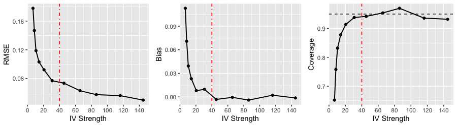
Figure S1: RMSE, bias and CI coverage of TSCI with different IV strengths. The red dashed line indicates the IV strength as 40. The black dashed line indicates the 95% coverage level.

We also use the setting with $a\in\{0.25,0.3,0.33\}$ to illustrate the bias of $\widehat{\beta}_{\rm init}(V)$ and the effect of the proposed bias correction in Figure 1 in the main paper.

D.2 Comparison with machine-learning IV

In the following, we compare our TSCI estimator with the MLIV estimator described in (29) while setting the full set of observed covariates as adjusted forms in our method. We use the exactly same setting in Section D.1. In Table S1, we compare TSCI with MLIV for different $n\in\{1000,3000,5000\}$ and different $a\in\{0.2,0.25,0.3,0.35\}$ with a larger value of $a$ corresponding to a stronger IV. We implement 500 rounds of simulations and report the average measure.

Table S1: Comparison of TSCI and MLIV with the treatment model fitted by RF. The columns indexed with “without self-prediction” stands for the split RF being implemented without self-prediction, while “with self-prediction” stands for the split RF being implemented with self-prediction. The columns indexed by “TSCI”, “Init”, “MLIV” correspond to our proposed TSCI estimator in (19), the initial estimator in (16), and the MLIV estimator in (29). The column indexed with “RMSE Ratio” represents the MSE ratio of the MLLV estimator to TSCI estimator; the column indexed with “IV Str” stands for our proposed IV strength in (22).

		without self-prediction					with self-prediction
		Bias			RMSE		Bias			RMSE
a	n	TSCI	Init	MLIV	Ratio	IV Str	TSCI	Init	MLIV	Ratio	IV Str
0.20	1000	0.17	0.30	-4.31	374.06	2.18	0.28	0.38	0.48	1.51	11.90
	3000	0.03	0.14	-0.15	2.94	12.11	0.17	0.29	0.45	2.17	42.06
	5000	0.01	0.10	-0.07	1.67	27.97	0.12	0.23	0.42	2.69	76.41
0.25	1000	0.06	0.18	-0.38	23.14	3.84	0.17	0.28	0.41	1.88	15.79
	3000	0.00	0.06	-0.05	1.37	30.35	0.08	0.17	0.35	2.97	74.95
	5000	0.00	0.04	-0.02	1.11	77.97	0.04	0.12	0.32	3.84	156.57
0.30	1000	0.02	0.09	-0.11	2.01	7.49	0.09	0.18	0.32	2.22	23.92
	3000	-0.00	0.02	-0.02	1.09	74.82	0.03	0.09	0.25	3.74	151.09
	5000	0.00	0.02	-0.01	1.06	194.74	0.01	0.06	0.21	4.51	316.40
0.35	1000	0.00	0.05	-0.05	1.29	14.32	0.04	0.11	0.24	2.57	41.62
	3000	-0.01	0.01	-0.01	0.99	144.72	0.01	0.04	0.17	3.55	255.65
	5000	-0.00	0.01	-0.01	1.00	337.34	0.01	0.04	0.16	4.44	526.98

In Table S1, we observe that the MLIV has a larger bias and standard error than TSCI, leading to an inflated MSE of MLIV. We have explained in Section 3.5 that this happens when the IV strength captured by RF is relatively weak. For a stronger IV (with $a=0.35$), when the sample size is 3000 or 5000 and the self-prediction is excluded, the MLIV and TSCI have comparable MSE, but our proposed TSCI estimator generally exhibits a smaller bias. Moreover, by comparing TSCI and initial estimators, our proposed bias correction step effectively removes the bias due to the high complexity of RF algorithm. Another interesting observation is that the removal of self-prediction helps reducing the bias of both TSCI and MLIV estimators for the reason of reducing the correlation between the ML predicted value and the unmeasured confounders.

We then show how the coefficient $c_{f}$ in (29) in the main paper inflates the estimation error of MLIV when IV is weak. In Figure S2, we display the distribution of TSCI and MLIV estimators in box plots and the frequency of $c_{f}$ in the histogram in the setting with $n=1000$ and $a=0.2$. We can see that there are certain proportion of the coefficient $c_{f}$ close to 0, which would inflate the estimator to extremely large values and thus increase the MLIV estimator variance when IV is weak.

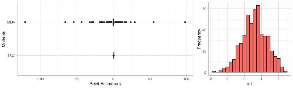
Figure S2: The left panel shows the boxplot of TSCI and MLIV estimators and the right panel shows the histogram of the coefficient $c_{f}$ of $\widehat{f}$ in the first stage regression $D\sim\widehat{f}+X$ in the MLIV method.

D.3 Multiple IV (with non-linearity)

In this section, we consider multiple IVs and compare TSCI with existing methods dealing with invalid IVs, including TSHT guo2018confidence and CIIV windmeijer2019confidence. We consider the setting with 10 IVs. With fixing the sample size $n=3000$, we generate $X^{*}_{i}\in\mathbb{R}^{p_{x}+p_{z}}$ following the multivariate normal distribution with zero mean and covariance $\Sigma$ where $\Sigma_{i,j}=0.5^{|i-j|}$ for $1\leq i,j\leq p_{x}+p_{z}$. We define the first $p_{z}$ columns of $X^{*}$ as IVs and denote it by $Z_{i}=X^{*}_{i,1:p_{z}}$. The remaining columns are defined as observed covariates, that is $X_{i}=X^{*}_{i,(p_{z}+1):(p_{z}+p_{x})}$. We generate errors $\{(\delta_{i},\epsilon_{i})^{\intercal}\}_{1\leq i\leq n}$ following the bivariate normal distribution with zero mean, unit variance and covariance as 0.5. We generate $\{D_{i},Y_{i}\}_{1\leq i\leq n}$ following $D_{i}=\sum_{j=1}^{p_{z}}|Z_{i,j}|+\sum_{j=1}^{p_{z}}\tanh(Z_{i,j})+1/2\cdot\sum_{j=1}^{p_{x}}X_{i,j}+\delta_{i}$ and $Y_{i}=D_{i}+Z_{i}\pi+1/2\cdot\sum_{j=1}^{p_{x}}X_{i,j}+\epsilon_{i}$ where the vector $\pi\in\mathbb{R}^{p_{z}}$ indicates the invalidity level of each IV. The $j$-th IV is valid if $\pi_{j}=0$; otherwise, it is invalid. A larger $|\pi_{j}|$ value indicates that the $j$-th IV is more severely invalid. We consider the following two settings,

• Setting D1: $\pi=a\cdot(0,0,0,0,{0.5},0.5,0.5,0.5,0.5,0.5)^{\intercal}$,

• Setting D2: $\pi=a\cdot(0,0,0,0,0.5,0.5,0.5,1,1,1)^{\intercal}$.

For Setting D1, neither the majority nor the plurality rule is satisfied. For Setting D2, the plurality rule is satisfied. We vary the value of $a\in\{0.1,0.2,\cdots,1\}$ to simulate the different levels of invalidity. We specify the sets of basis as $\mathcal{V}_{0}=\{\overrightarrow{\bf w}(x)\}$ with $\overrightarrow{\bf w}(x)=\{1,x_{1},\cdots,x_{p_{x}}\}$, $\mathcal{V}_{1}=\{\mathbf{z},\overrightarrow{\bf w}(x)\}$ and $\mathcal{V}_{2}=\{\mathbf{z},\mathbf{z}^{2},\overrightarrow{\bf w}(x)\}$ with $\mathbf{z}^{2}=\{z_{1}^{2},\cdots,z_{10}^{2}\}$. We run 500 rounds of simulation and report the results in Figure S3.

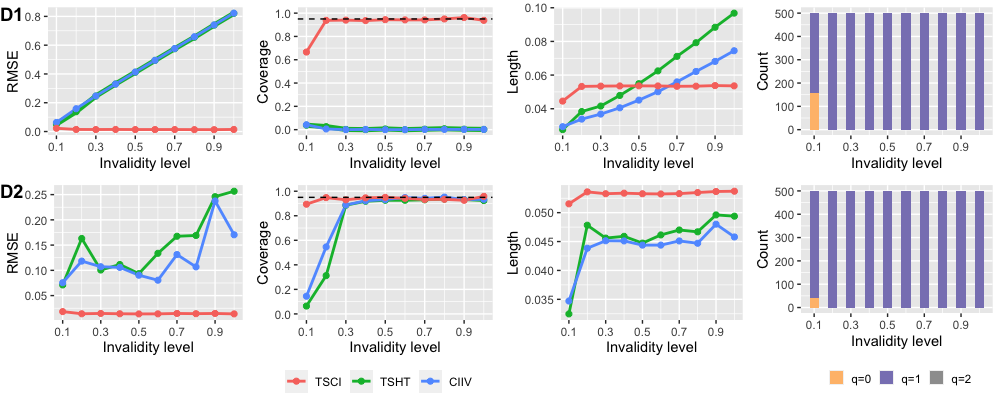
Figure S3: Comparison of TSCI with TSHT and CIIV in terms of RMSE, CI coverage and length under Settings D1 and D2. Setting D1 corresponds to a setting that the plurality rule fails while Setting D2 corresponds to a setting that the plurality holds. The stacked bar charts in the last column show the basis selection of TSCI where $\mathcal{V}_{q=1}$ is the oracle basis set. “TSCI” is our proposed method detailed in Algorithm 1. “TSHT” and “CIIV” are the methods proposed in guo2018confidence and windmeijer2019confidence.

In Setting D1, neither the majority rule nor the plurality rule is satisfied, so TSHT and CIIV cannot select valid IVs and do not achieve a desired coverage level of 95%. In contrast, TSCI is able to detect the existing invalidity and obtain valid inference. When the invalidity level is low (with $a=0.1$), TSCI may not be able to identify the invalidity and thus lead to coverage below 95%.

In Setting D2, TSCI achieves the desired coverage level while TSHT and CIIV achieve the desired coverage for a relatively large invalidity level. When the invalidity level is low, say $a=0.1$ and $a=0.2$, TSHT and CIIV are significantly impacted by locally invalid IVs and generate poor coverage. In comparison to TSHT and CIIV, TSCI provides much more robust performance to the low invalidity levels because it evaluates the total invalidity levels accumulated by all ten invalid IVs.

D.4 Additional Results in Section 5.2

In this section, we further report the additional results for Setting B1 and results for Setting B2, and introduce a setting with binary IV denoted as Setting B3.

For Setting B1, we report the coverage for Vio=2 in Table S2 and we further report the mean absolute bias and the confidence interval length in for both violation forms in Tables S3 and S4, respectively. In Table S3, TSLS has a large bias due to the existence of invalid IVs; even in the oracle setting with the prior knowledge of the best $\mathcal{V}_{q}$ approximating $g$, RF-Full, and RF-Plug have a large bias. Compared with RF-Init, TSCI corrects the bias effectively and thus have the desired 95% coverage. In Table S4, the CI of TSCI is shorter than the oracle method in settings with small sample size or weak interaction strength, because it fails to select the correct violation forms.

			TSCI-RF				Proportions of selection				TSLS	Other RF(oracle)
vio	a	n	Oracle	Comp	Robust	Invalidity	$\widehat{q}_{c}=0$	$\widehat{q}_{c}=1$	$\widehat{q}_{c}=2$	$\widehat{q}_{c}=3$		Init	Plug	Full
2	0.0	1000	0.92	0.01	0.01	0.00	1.00	0.00	0.00	0.00	0.00	0.82	0.30	0.01
		3000	0.94	0.94	0.94	1.00	0.00	0.00	1.00	0.00	0.00	0.91	0.63	0.00
		5000	0.94	0.94	0.94	1.00	0.00	0.00	1.00	0.00	0.00	0.88	0.77	0.00
	0.5	1000	0.92	0.11	0.12	0.21	0.79	0.08	0.13	0.00	0.00	0.86	0.49	0.01
		3000	0.94	0.93	0.92	1.00	0.00	0.00	0.97	0.03	0.00	0.90	0.37	0.00
		5000	0.94	0.94	0.94	1.00	0.00	0.00	0.99	0.01	0.00	0.88	0.03	0.00
	1.0	1000	0.95	0.89	0.89	0.96	0.04	0.02	0.93	0.01	0.00	0.89	0.40	0.01
		3000	0.93	0.93	0.93	1.00	0.00	0.00	0.99	0.01	0.00	0.92	0.00	0.00
		5000	0.93	0.93	0.93	1.00	0.00	0.00	1.00	0.00	0.00	0.90	0.00	0.00

Table S2: Coverage (at nominal level 0.95) for Setting B1 with Vio=2. The columns indexed with “TSCI-RF” correspond to our proposed TSCI with random forests, where the columns indexed with “Oracle”, “Comp” and “Robust” correspond to the estimators with $\mathcal{V}_{q}$ selected by the oracle knowledge, the comparison method, and the robust method. The column indexed with “Invalidity” reports the proportion of detecting the proposed IV as invalid. The columns indexed with “Proportions of selection” reports the proportions of basis sets $\mathcal{V}_{q}$ for $0\leq q\leq 3$ selected by TSCI-RF. The column indexed with “TSLS” corresponds to the TSLS estimator. The columns indexed with “Init”, “Plug”, “Full” correspond to the RF estimators without bias correction, the plug-in RF estimator and the no data-splitting RF estimator, with the oracle knowledge of the best $\mathcal{V}_{q}$.

			TSCI-RF				Proportions of selection				TSLS	Other RF(oracle)
vio	a	n	Oracle	Comp	Robust	Invalidity	$\widehat{q}_{c}=0$	$\widehat{q}_{c}=1$	$\widehat{q}_{c}=2$	$\widehat{q}_{c}=3$		Init	Plug	Full
1	0.0	1000	0.02	0.53	0.53	0.01	0.99	0.01	0.00	0.00	0.56	0.13	0.48	0.30
		3000	0.01	0.01	0.01	1.00	0.00	0.84	0.16	0.00	0.56	0.04	0.14	0.25
		5000	0.00	0.00	0.00	1.00	0.00	0.85	0.15	0.00	0.56	0.03	0.05	0.23
	0.5	1000	0.01	0.26	0.25	0.24	0.76	0.24	0.01	0.00	0.33	0.08	0.24	0.22
		3000	0.00	0.00	0.00	1.00	0.00	0.97	0.02	0.01	0.33	0.03	0.16	0.19
		5000	0.00	0.00	0.00	1.00	0.00	0.98	0.01	0.01	0.33	0.02	0.22	0.18
	1.0	1000	0.00	0.01	0.01	0.95	0.05	0.93	0.01	0.00	0.23	0.04	0.15	0.13
		3000	0.00	0.00	0.00	1.00	0.00	0.99	0.01	0.00	0.23	0.01	0.38	0.11
		5000	0.00	0.00	0.00	1.00	0.00	0.98	0.02	0.01	0.23	0.01	0.37	0.10
2	0.0	1000	0.00	0.54	0.54	0.00	1.00	0.00	0.00	0.00	0.56	0.11	0.53	0.29
		3000	0.00	0.00	0.00	1.00	0.00	0.00	1.00	0.00	0.56	0.05	0.13	0.25
		5000	0.00	0.00	0.00	1.00	0.00	0.00	1.00	0.00	0.56	0.03	0.05	0.23
	0.5	1000	0.01	0.38	0.38	0.21	0.79	0.08	0.13	0.00	0.33	0.08	0.34	0.23
		3000	0.00	0.00	0.01	1.00	0.00	0.00	0.97	0.03	0.33	0.03	0.19	0.20
		5000	0.00	0.00	0.01	1.00	0.00	0.00	0.99	0.01	0.33	0.03	0.29	0.19
	1.0	1000	0.01	0.04	0.04	0.96	0.04	0.02	0.93	0.01	0.23	0.04	0.25	0.15
		3000	0.00	0.00	0.00	1.00	0.00	0.00	0.99	0.01	0.23	0.02	0.52	0.12
		5000	0.00	0.00	0.00	1.00	0.00	0.00	1.00	0.00	0.23	0.01	0.48	0.11

Table S3: Absolute Bias for Setting B1. The columns indexed with “TSCI-RF” correspond to our proposed TSCI with random forests, where the columns indexed with “Oracle”, “Comp” and “Robust” correspond to estimators with $\mathcal{V}_{q}$ selected by the oracle knowledge, the comparison method, and the robust method. The column indexed with “Invalidity” reports the proportion of detecting the proposed IV as invalid. The columns indexed with “Proportions of selection” reports the proportions of basis sets $\mathcal{V}_{q}$ selected by TSCI-RF using the comparison method. The columns indexed with “TSLS” corresponds to the TSLS estimator. The columns indexed with “Init”, “Plug”, “Full” correspond to the RF estimators without bias correction, the plug-in RF estimator and the no data-splitting RF estimator, with the oracle knowledge of the best $\mathcal{V}_{q}$.

			TSCI-RF				Proportions of selection				TSLS	Other RF(oracle)
vio	a	n	Oracle	Comp	Robust	Invalidity	$\widehat{q}_{c}=0$	$\widehat{q}_{c}=1$	$\widehat{q}_{c}=2$	$\widehat{q}_{c}=3$		Init	Plug	Full
1	0.0	1000	0.49	0.11	0.11	0.01	0.99	0.01	0.00	0.00	0.08	0.49	0.82	0.22
		3000	0.32	0.32	0.32	1.00	0.00	0.84	0.16	0.00	0.05	0.32	0.38	0.14
		5000	0.23	0.23	0.23	1.00	0.00	0.85	0.15	0.00	0.04	0.23	0.27	0.11
	0.5	1000	0.38	0.13	0.14	0.24	0.76	0.24	0.01	0.00	0.05	0.38	0.60	0.19
		3000	0.22	0.22	0.23	1.00	0.00	0.97	0.02	0.01	0.03	0.22	0.26	0.11
		5000	0.17	0.17	0.17	1.00	0.00	0.98	0.01	0.01	0.02	0.17	0.19	0.09
	1.0	1000	0.25	0.24	0.24	0.95	0.05	0.93	0.01	0.00	0.04	0.25	0.33	0.14
		3000	0.13	0.13	0.13	1.00	0.00	0.99	0.01	0.00	0.02	0.13	0.18	0.08
		5000	0.10	0.10	0.10	1.00	0.00	0.98	0.02	0.01	0.02	0.10	0.13	0.06
2	0.0	1000	0.49	0.17	0.17	0.00	1.00	0.00	0.00	0.00	0.12	0.49	0.85	0.21
		3000	0.31	0.31	0.31	1.00	0.00	0.00	1.00	0.00	0.07	0.31	0.38	0.14
		5000	0.23	0.23	0.23	1.00	0.00	0.00	1.00	0.00	0.06	0.23	0.27	0.11
	0.5	1000	0.38	0.16	0.16	0.21	0.79	0.08	0.13	0.00	0.07	0.38	0.70	0.18
		3000	0.23	0.23	0.26	1.00	0.00	0.00	0.97	0.03	0.04	0.23	0.28	0.11
		5000	0.17	0.17	0.21	1.00	0.00	0.00	0.99	0.01	0.03	0.17	0.20	0.09
	1.0	1000	0.24	0.24	0.24	0.96	0.04	0.02	0.93	0.01	0.05	0.24	0.40	0.14
		3000	0.13	0.13	0.13	1.00	0.00	0.00	0.99	0.01	0.03	0.13	0.22	0.08
		5000	0.10	0.10	0.11	1.00	0.00	0.00	1.00	0.00	0.02	0.10	0.15	0.06

Table S4: Average CI length for Setting B1. The columns indexed with “TSCI-RF” correspond to TSCI with random forests, where the columns indexed with “Oracle”, “Comp” and “Robust” correspond to estimators with $\mathcal{V}_{q}$ selected by the oracle knowledge, the comparison method, and the robust method. The column indexed with “Invalidity” reports the proportion of detecting the proposed IV as invalid. The columns indexed with “Proportions of selection” reports the proportions of basis sets $\mathcal{V}_{q}$ selected by TSCI-RF using the comparison method. The columns indexed with “TSLS” corresponds to the TSLS estimator. The columns indexed with “Init”, “Plug”, “Full” correspond to the RF estimators without bias correction, the plug-in RF estimator and the no data-splitting RF estimator, with the oracle knowledge of the best $\mathcal{V}_{q}$.

			TSCI-RF				Proportions of selection				TSLS	Other RF(oracle)
vio	a	n	Oracle	Comp	Robust	Invalidity	$\widehat{q}_{c}=0$	$\widehat{q}_{c}=1$	$\widehat{q}_{c}=2$	$\widehat{q}_{c}=3$		Init	Plug	Full
1	0	1000	0.84	0.84	0.84	1.00	0.00	1.00	0.00	0.00	0.58	0.81	0.16	0.00
		3000	0.93	0.93	0.94	1.00	0.00	0.96	0.04	0.00	0.11	0.91	0.00	0.00
		5000	0.93	0.94	0.94	1.00	0.00	0.95	0.05	0.00	0.01	0.93	0.00	0.00
	0.5	1000	0.94	0.94	0.95	1.00	0.00	0.95	0.04	0.01	0.00	0.88	0.00	0.01
		3000	0.93	0.93	0.92	1.00	0.00	0.95	0.05	0.00	0.00	0.92	0.00	0.01
		5000	0.93	0.93	0.93	1.00	0.00	0.99	0.01	0.00	0.00	0.92	0.00	0.00
	1	1000	0.94	0.94	0.95	1.00	0.00	0.98	0.01	0.00	0.00	0.92	0.00	0.01
		3000	0.95	0.96	0.96	1.00	0.00	0.98	0.02	0.00	0.00	0.93	0.00	0.00
		5000	0.93	0.93	0.93	1.00	0.00	0.99	0.01	0.00	0.00	0.91	0.00	0.00
2	0	1000	0.84	0.17	0.17	0.99	0.01	0.97	0.02	0.00	0.55	0.16	0.13	0.00
		3000	0.96	0.96	0.94	1.00	0.00	0.00	0.99	0.01	0.14	0.93	0.00	0.00
		5000	0.95	0.95	0.94	1.00	0.00	0.00	0.99	0.01	0.02	0.92	0.00	0.01
	0.5	1000	0.95	0.73	0.72	0.92	0.08	0.17	0.70	0.05	0.00	0.68	0.00	0.03
		3000	0.94	0.94	0.94	1.00	0.00	0.00	0.95	0.05	0.00	0.93	0.00	0.00
		5000	0.95	0.95	0.95	1.00	0.00	0.00	0.98	0.02	0.00	0.92	0.00	0.00
	1	1000	0.96	0.95	0.96	1.00	0.00	0.01	0.93	0.06	0.00	0.94	0.00	0.01
		3000	0.96	0.95	0.94	1.00	0.00	0.00	0.95	0.05	0.00	0.93	0.00	0.00
		5000	0.96	0.96	0.95	1.00	0.00	0.00	0.97	0.03	0.00	0.95	0.00	0.00

Table S5: CI coverage for Setting B2. The columns indexed with “TSCI-RF” correspond to TSCI with random forests, where the columns indexed with “Oracle”, “Comp” and “Robust” correspond to estimators with $\mathcal{V}_{q}$ selected by the oracle knowledge, the comparison method, and the robust method. The column indexed with “Invalidity” reports the proportion of detecting the proposed IV as invalid. The columns indexed with “Proportions of selection” reports the proportions of basis sets $\mathcal{V}_{q}$ selected by TSCI-RF using the comparison method. The columns indexed with “TSLS” corresponds to the TSLS estimator. The columns indexed with “Init”, “Plug”, “Full” correspond to the RF estimators without bias correction, the plug-in RF estimator and the no data-splitting RF estimator, with the oracle knowledge of the best $\mathcal{V}_{q}$.

For Setting B2, we report the empirical coverage in Table S5 which are generally similar to those for Setting B1.

To approximate the real data analysis in Section 6, we further generate a binary IV as $Z_{i}={\bf 1}(\Phi(X^{*}_{i,6})>0.6)$ and the covariates $X_{i,j}=X^{*}_{i,j}$ for $1\leq i\leq n$ and $1\leq j\leq 5.$ We consider the following models for $f(Z_{i},X_{i})$ and $g(Z_{i},X_{i})$,

• Setting B3 (binary IV): $f(Z_{i},X_{i})=Z_{i}\cdot(1+a\sum_{j=1}^{4}X_{ij}(1+X_{i,j+1}))-3/10\cdot\sum_{i=1}^{5}X_{ij}$ and $g(Z_{i},X_{i})=Z_{i}+1/2\cdot Z_{i}\cdot(\sum_{i=1}^{3}X_{ij})).$

Compared to Settings B1 and B2, the outcome model in Setting B3 involves the interaction between $Z_{i}$ and $X_{i}$ while the treatment model involves a more complicated interaction term, whose strength is controlled by $a$. We specify $\mathcal{V}_{0}=\{\overrightarrow{\bf w}(x)\}$ with $\overrightarrow{\bf w}(x)=\{1,x_{1},\cdots,x_{5}\}$ and $\mathcal{V}_{1}=\mathcal{V}_{0}\cup\{z,z\cdot x_{1},\cdots,z\cdot x_{5}\}$. With the specified basis sets, we implement TSCI with random forests as detailed in Algorithm 1 in the main paper. In Table S6, we demonstrate our proposed TSCI method for Setting B3. The observations are coherent with those for Settings B1 and B2. The main difference between the binary IV (Setting B3) and the continuous IV (Settings B1 and B2) is that the treatment effect is not identifiable for $a=0$, which happens only for the binary IV setting. However, with a non-zero interaction and a relatively large sample size, our proposed TSCI methods achieve the desired coverage. We also observe that the bias correction is effective and improves the coverage when the interaction $a$ is relatively small.

		TSCI-RF										RF-Init
		Bias			Length			Coverage			Invalidity	Bias	Coverage
a	n	Orac	Comp	Robust	Orac	Comp	Robust	Orac	Comp	Robust		Orac	Orac
0.25	1000	0.01	0.56	0.56	0.42	0.23	0.23	0.90	0.28	0.28	0.31	0.10	0.82
	3000	0.00	0.01	0.01	0.23	0.23	0.23	0.95	0.95	0.95	0.99	0.05	0.84
	5000	0.00	0.00	0.00	0.18	0.18	0.18	0.94	0.94	0.94	1.00	0.03	0.86
0.50	1000	0.00	0.02	0.02	0.22	0.22	0.22	0.93	0.90	0.90	0.97	0.04	0.90
	3000	-0.00	-0.00	-0.00	0.12	0.12	0.12	0.93	0.93	0.93	1.00	0.02	0.89
	5000	0.00	0.00	0.00	0.09	0.09	0.09	0.95	0.95	0.95	1.00	0.02	0.89
0.75	1000	0.00	0.00	0.00	0.15	0.15	0.15	0.92	0.90	0.90	0.99	0.02	0.91
	3000	0.00	0.00	0.00	0.08	0.08	0.08	0.94	0.94	0.94	1.00	0.01	0.89
	5000	-0.00	-0.00	-0.00	0.06	0.06	0.06	0.93	0.93	0.93	1.00	0.01	0.91

Table S6: Bias, length, and coverage (at nominal level 0.95) for Setting B3. The columns indexed with “TSCI-RF” corresponds to our proposed TSCI with random forests, where the columns indexed with “Bias”, “Length”, and “Coverage” correspond to the absolute bias of the point estimator, the length and empirical coverage of the constructed CI respectively. The columns indexed with “Oracle”, “Comp” and “Robust” correspond to TSCI estimators with $\mathcal{V}_{q}$ selected by the oracle knowledge, the comparison method, and the robust method. The column indexed with “Invalidity” reports the proportion of detecting the proposed IV as invalid. The columns indexed with “RF-Init” correspond to the RF estimators without bias correction but with the oracle knowledge of the best $\mathcal{V}_{q}$.

D.5 Binary Treatment

We consider the binary treatment setting and explore the finite-sample performance of our proposed TSCI method. We consider the outcome model $Y_{i}=D_{i}\beta+Z_{i}+0.2\cdot\sum_{j=1}^{p}{X_{ij}}+\epsilon_{i}$ with $\beta=1$ and $p_{x}=20.$ We generate $\epsilon_{i}$ and $\delta_{i}$ following bivariate normal distribution with zero mean, unit variance and covariance as 0.5. We generate the binary treatment $D_{i}$ with the conditional mean as

$${\mathbf{E}}(D_{i}\mid Z_{i},X_{i})=\frac{\exp(f(Z_{i},X_{i})+\delta_{i})}{1+\exp(f(Z_{i},X_{i})+\delta_{i})},$$

where $f(Z_{i},X_{i})$ is specified in the following two ways.

• Setting 1 (continuous IV): generate $Z_{i},X_{i}$ following Section 5.2. $f(Z_{i},X_{i})=-25/12+Z_{i}+Z_{i}^{2}+1/8\cdot Z_{i}^{4}+Z_{i}\cdot(a\cdot\sum_{j=1}^{5}X_{i,j})-3/10\cdot\sum_{j=1}^{p_{x}}X_{i,j}$.

• Setting 2 (binary IV): generate $f(Z_{i},X_{i})=Z_{i}\cdot(1+a\cdot\sum_{j=1}^{5}X_{ij})-\sum_{j=1}^{p}0.3X_{ij}$.

			TSCI-RF										RF-Init		TSCI-RF
			Bias			Length			Coverage			Invalidity	Bias	Coverage	Weak IV
Setting	a	n	Orac	Comp	Robust	Orac	Comp	Robust	Orac	Comp	Robust		Orac	Orac
		1000	0.00	0.00	0.00	1.08	1.08	1.08	0.92	0.92	0.92	1.00	0.05	0.94	0.99
		3000	0.01	0.01	0.00	0.59	0.59	0.61	0.94	0.93	0.93	1.00	0.00	0.95	0.00
	0.0	5000	0.00	0.00	0.01	0.44	0.45	0.89	0.94	0.93	0.95	1.00	0.01	0.94	0.00
		1000	0.03	0.03	0.03	1.12	1.12	1.12	0.90	0.90	0.90	1.00	0.07	0.94	0.99
		3000	0.00	0.00	0.00	0.62	0.62	0.62	0.93	0.93	0.93	1.00	0.01	0.94	0.00
	0.5	5000	0.00	0.00	0.01	0.45	0.45	0.68	0.94	0.93	0.93	1.00	0.01	0.94	0.00
		1000	0.01	0.01	0.01	1.22	1.22	1.22	0.92	0.92	0.92	1.00	0.04	0.95	0.99
		3000	0.01	0.01	0.00	0.66	0.66	0.67	0.95	0.95	0.95	1.00	0.01	0.96	0.00
	1.0	5000	0.00	0.00	0.00	0.49	0.49	0.62	0.93	0.93	0.93	1.00	0.01	0.94	0.00
		1000	0.01	0.01	0.01	1.30	1.30	1.30	0.89	0.89	0.89	1.00	0.06	0.94	1.00
		3000	0.00	0.00	0.00	0.73	0.73	0.74	0.95	0.95	0.95	1.00	0.01	0.96	0.01
1	1.5	5000	0.00	0.00	0.01	0.53	0.54	0.82	0.93	0.92	0.93	1.00	0.01	0.94	0.00
		1000	0.37	0.37	0.37	1.62	1.62	1.62	0.66	0.66	0.66	0.93	0.41	0.78	1.00
		3000	0.41	0.41	0.41	1.25	1.25	1.25	0.60	0.60	0.60	1.00	0.42	0.72	1.00
	0.0	5000	0.35	0.35	0.35	1.05	1.05	1.05	0.61	0.61	0.61	1.00	0.40	0.65	1.00
		1000	0.30	0.30	0.30	1.21	1.21	1.21	0.65	0.65	0.65	1.00	0.36	0.77	1.00
		3000	0.21	0.21	0.21	1.18	1.18	1.18	0.73	0.73	0.73	1.00	0.29	0.83	1.00
	0.5	5000	0.10	0.10	0.10	1.09	1.09	1.09	0.82	0.82	0.82	1.00	0.22	0.89	1.00
		1000	0.16	0.20	0.16	1.35	1.30	1.35	0.77	0.77	0.77	0.93	0.26	0.87	1.00
		3000	0.03	0.03	0.03	1.11	1.10	1.11	0.88	0.88	0.88	0.99	0.11	0.94	1.00
	1.0	5000	0.00	0.00	0.00	0.92	0.92	0.92	0.89	0.89	0.89	1.00	0.07	0.93	0.57
		1000	0.06	0.22	0.06	1.59	1.31	1.59	0.83	0.67	0.83	0.75	0.18	0.93	1.00
		3000	0.01	0.02	0.01	1.14	1.13	1.14	0.90	0.90	0.90	0.98	0.08	0.93	0.87
2	1.5	5000	0.00	0.00	0.00	0.91	0.91	0.91	0.93	0.93	0.93	1.00	0.04	0.95	0.02

Table S7: Bias, length, and coverage (at nominal level 0.95) for binary treatment model with Model 1 (continuous IV) and Model 4 (binary IV). The columns indexed with “TSCI-RF” corresponds to our proposed TSCI with the random forests, where the columns indexed with “Bias”, “Length”, and “Coverage” correspond to the absolute bias of the point estimator, the length and empirical coverage of the constructed confidence interval respectively. The columns indexed with “Oracle”, “Comp” and “Robust” correspond to the TSCI estimators with $\mathcal{V}_{q}$ selected by the oracle knowledge, the comparison method, and the robust method. The column indexed with “Invalidity” reports the proportion of detecting the proposed IV as invalid. The columns indexed with “RF-Init” correspond to the RF estimators without bias correction but with the oracle knowledge of the best $\mathcal{V}_{q}$. The column indexed with “Weak IV” stands for the proportion out of 500 simulations reporting $Q_{\max}<1.$

The binary treatment result is summarized in Table S7. The main observation is similar to those for the continuous treatment reported in the main paper. We shall point out the major differences in the following. The settings with the binary treatment are in general more challenging since the IV strength is relatively weak. To measure this, we have reported the column indexed with “weak IV” standing for the proportion of simulations with $Q_{\max}=0.$ For settings where our proposed generalized IV strength is strong such that $Q_{\max}\geq 1$, our proposed TSCI method achieves the desired coverage level. Even when the generalized IV strength leads to $Q_{\max}<1,$ our proposed (oracle) TSCI may still achieve the desired coverage level for setting 1.

Appendix E Additional Results for Real Data Analysis

This section contains the additional results for the real data analysis. In Figure S4, we first show the importance score of all variables in random forests, based on which the six most important covariates are selected to construct the basis set $\mathcal{V}_{1}$ in Section 6.

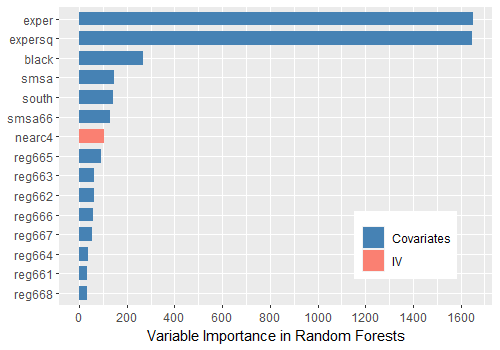
Figure S4: The importance score of each variable in random forest fitting.

E.1 Other specifications of $\mathcal{V}_{2}$

In the following, in addition to the basis set $\mathcal{V}_{2}$ considered in Section 6, we consider three more specifications of $\mathcal{V}_{2}$, as detailed in Table S8, and test the robustness of TSCI’s selection process.

$\mathcal{V}_{2}$	$\mathcal{V}_{1}\cup${nearc4$\cdot$reg1, nearc4$\cdot$reg2, nearc4$\cdot$reg3, nearc4$\cdot$reg4,nearc4$\cdot$reg5, nearc4$\cdot$reg6, nearc4$\cdot$reg7, nearc4$\cdot$reg8}
$\mathcal{V}_{2}^{(1)}$	$\mathcal{V}_{1}\cup\{\texttt{nearc4}\cdot\texttt{exper}^{3}\}$
$\mathcal{V}_{2}^{(2)}$	$\mathcal{V}_{1}\cup\{\texttt{nearc4}\cdot\texttt{exper}\cdot\texttt{black},\texttt{nearc4}\cdot\texttt{exper}\cdot\texttt{south},\texttt{nearc4}\cdot\texttt{exper}\cdot\texttt{smsa},\texttt{nearc4}\cdot\texttt{exper}\cdot\texttt{smsa66}$, $\texttt{nearc4}\cdot\texttt{expersq}\cdot\texttt{black},\texttt{nearc4}\cdot\texttt{expersq}\cdot\texttt{south},\texttt{nearc4}\cdot\texttt{expersq}\cdot\texttt{smsa},\texttt{nearc4}\cdot\texttt{expersq}\cdot\texttt{smsa66}$, $\texttt{nearc4}\cdot\texttt{black}\cdot\texttt{south},\texttt{nearc4}\cdot\texttt{black}\cdot\texttt{smsa},\texttt{nearc4}\cdot\texttt{black}\cdot\texttt{smsa66}$, $\texttt{nearc4}\cdot\texttt{south}\cdot\texttt{smsa},\texttt{nearc4}\cdot\texttt{south}\cdot\texttt{smsa66},\texttt{nearc4}\cdot\texttt{smsa}\cdot\texttt{smsa66}\}$
$\mathcal{V}_{2}^{(3)}$	$\mathcal{V}_{1}\cup\{\texttt{nearc4}\cdot\texttt{exper}^{3},\texttt{nearc4}\cdot\texttt{exper}\cdot\texttt{black},\texttt{nearc4}\cdot\texttt{exper}\cdot\texttt{south},\texttt{nearc4}\cdot\texttt{exper}\cdot\texttt{smsa},\texttt{nearc4}\cdot\texttt{exper}\cdot\texttt{smsa66}$, $\texttt{nearc4}\cdot\texttt{expersq}\cdot\texttt{black},\texttt{nearc4}\cdot\texttt{expersq}\cdot\texttt{south},\texttt{nearc4}\cdot\texttt{expersq}\cdot\texttt{smsa},\texttt{nearc4}\cdot\texttt{expersq}\cdot\texttt{smsa66}$, $\texttt{nearc4}\cdot\texttt{black}\cdot\texttt{south},\texttt{nearc4}\cdot\texttt{black}\cdot\texttt{smsa},\texttt{nearc4}\cdot\texttt{black}\cdot\texttt{smsa66}$, $\texttt{nearc4}\cdot\texttt{south}\cdot\texttt{smsa},\texttt{nearc4}\cdot\texttt{south}\cdot\texttt{smsa66},\texttt{nearc4}\cdot\texttt{smsa}\cdot\texttt{smsa66}\}$

Table S8: Different specifications of the second basis set $\mathcal{V}_{2}$. $\mathcal{V}_{2}$ is the specification we used in Section 6. $\mathcal{V}_{2}^{(1)}$ contains the two-way interaction of the IV with covariates exper and expersq and $\mathcal{V}_{1}$; $\mathcal{V}_{2}^{(2)}$ includes all the two-way interactions of the IV with 6 most important covariates excluding the interaction of the IV with exper, expersq; $\mathcal{V}_{2}^{(3)}$ includes all the two-way interactions of the IV with 6 most important covariates.

We implement TSCI with random forests as detailed in Algorithm 1 with specifying $\mathcal{V}_{0},\mathcal{V}_{1}$ as in Section 6 and different $\mathcal{V}_{2}$ in Table S8. We observe that the point estimators and confidence intervals are relatively stable even with different specifications of $\mathcal{V}_{2}.$

Identifications	TSCI		Proportions of selection			Prob($Q_{\text{max}}>\widehat{q}_{c}$)	IV str.
	Estimate	CI	$\widehat{q}_{c}=0$	$\widehat{q}_{c}=1$	$\widehat{q}_{c}=2$
TSCI-$\mathcal{V}_{2}$	0.0604	(0.0294, 0.0914)	59.2%	38.2%	2.6%	93.6%	112.7950
TSCI-$\mathcal{V}_{2}^{(1)}$	0.0575	(0.0263, 0.0886)	40.0%	58.6%	1.4%	2.3%	111.8835
TSCI-$\mathcal{V}_{2}^{(2)}$	0.0614	(0.0303, 0.0916)	55.0%	40.0%	5.0%	72.9%	111.6233
TSCI-$\mathcal{V}_{2}^{(3)}$	0.0575	(0.0268, 0.0891)	39.2%	60.6%	0.2%	0%	113.0134

Table S9: Inference and basis selection of TSCI with different identifications of $\mathcal{V}_{2}$. The columns indexed with “Inference” correspond to the point estimators and the CI reported by TSCI in Algorithm 1 with $\mathcal{V}_{\widehat{q}_{c}}$. The columns indexed with “Proportions of selection” correspond to proportions of different selections over 500 rounds of simulations. The column indexed with “Prob($Q_{\text{max}}>\widehat{q}_{c}$)” indicates the proportion of $Q_{\text{max}}>\widehat{q}_{c}$. This case means that TSCI is able to selects $\widehat{q}_{c}$ without any weak IV constraints. The last column shows the average IV strength for TSCI estimators.

E.2 Falsification Argument of Condition 1

We propose in the following a falsification argument regarding Condition 1 for the data analysis. Particularly, we demonstrate that the regression model using covariates belonging to $\mathcal{V}_{1}$ provides a good approximation of $g(z,x)$ but not $f(z,x)$. With the TSCI estimator $\widehat{\beta}_{\mathcal{V}_{\widehat{q}_{c}}}$, we construct the pseudo outcome $\widetilde{Y}=Y-D\widehat{\beta}_{\mathcal{V}_{\widehat{q}_{c}}}$ and if $\widehat{\beta}_{\mathcal{V}_{\widehat{q}_{c}}}$ is a reasonably good estimator of $\beta$, then the pseudo outcome $\{\widetilde{Y}_{i}\}_{1\leq i\leq n}$ can be used as proxies of $\{g(Z_{i},X_{i})\}_{1\leq i\leq n}.$ Then we implement two OLS regressions of the pseudo outcome on the covariates in $\mathcal{V}_{1}$ and $\mathcal{V}_{2}$ as defined in Table 3. In addition, we build a random forests prediction model for the pseudo outcome with the predictors $Z_{i}$ and $X_{i}$. To evaluate the performance, we split the data into a training set $\mathcal{A}_{2}$ and a test set $\mathcal{A}_{1}$ as in Section 3.1, where test set $\mathcal{A}_{1}$ is used to estimate the out-of-sample MSE of the model constructed with the training set $\mathcal{A}_{2}$. We randomly split the data 500 times and report the violin plot of 500 MSE on the left panel of Figure S5. Since our specified basis set $\mathcal{V}_{1}$ leads to a nearly similar prediction performance as the random forests prediction model, this suggests that $\mathcal{V}_{1}$ provides a good approximation of the function $g(\cdot)$ if the TSCI estimator is accurate. In comparison, we use the treatment variable to replace the pseudo outcome and compare the MSE of the three prediction models. On the right panel of Figure S5, the random forests prediction model performs much better than the OLS with covariates in $\mathcal{V}_{1}$ and $\mathcal{V}_{2}$, indicating that $\mathcal{V}_{1}$ does not provide a good approximation for $f(\cdot)$ in the treatment model.

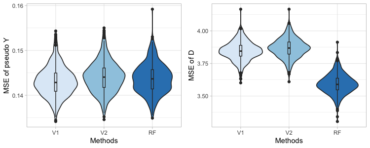
Figure S5: Violin plot of MSE for different prediction models, where the left and right panels correspond to using $\widetilde{Y}_{i}=Y_{i}-D_{i}\widehat{\beta}_{\mathcal{V}_{\widehat{q}_{c}}}$ and $D_{i}$ as the regression outcome variables, respectively. On both panels, “V1”, “V2”, and “RF” respectively stand for OLS regression with $\mathcal{V}_{1}$, $\mathcal{V}_{2}$, and random forests with $Z_{i}$ and $X_{i}$, where $\mathcal{V}_{1}$ and $\mathcal{V}_{2}$ are specified in Table 3.

chicago.bst IVRef

References

• Amemiya (1974) Amemiya, T. (1974). The nonlinear two-stage least-squares estimator. J. Econom. 2(2), 105–110.
• Angrist et al. (1999) Angrist, J. D., G. W. Imbens, and A. B. Krueger (1999). Jackknife instrumental variables estimation. J. Appl. Econ. 14(1), 57–67.
• Angrist and Lavy (1999) Angrist, J. D. and V. Lavy (1999). Using maimonides’ rule to estimate the effect of class size on scholastic achievement. Q. J. Econ. 114(2), 533–575.
• Angrist and Pischke (2009) Angrist, J. D. and J.-S. Pischke (2009). Mostly harmless econometrics: An empiricist’s companion. Princeton university press.
• Athey and Imbens (2016) Athey, S. and G. Imbens (2016). Recursive partitioning for heterogeneous causal effects. Proc. Natl. Acad. Sci. 113(27), 7353–7360.
• Athey et al. (2019) Athey, S., J. Tibshirani, and S. Wager (2019). Generalized random forests. Ann. Stat. 47(2), 1148–1178.
• Bach et al. (2021) Bach, P., V. Chernozhukov, M. S. Kurz, and M. Spindler (2021). DoubleML – An object-oriented implementation of double machine learning in R. arXiv:2103.09603 [stat.ML].
• Bekker and Crudu (2015) Bekker, P. A. and F. Crudu (2015). Jackknife instrumental variable estimation with heteroskedasticity. J. Econom. 185(2), 332–342.
• Belloni et al. (2012) Belloni, A., D. Chen, V. Chernozhukov, and C. Hansen (2012). Sparse models and methods for optimal instruments with an application to eminent domain. Econometrica 80(6), 2369–2429.
• Bowden et al. (2015) Bowden, J., G. Davey Smith, and S. Burgess (2015). Mendelian randomization with invalid instruments: effect estimation and bias detection through egger regression. Int. J. Epidemiol. 44(2), 512–525.
• Bowden et al. (2016) Bowden, J., G. Davey Smith, P. C. Haycock, and S. Burgess (2016). Consistent estimation in mendelian randomization with some invalid instruments using a weighted median estimator. Genet. Epidemiol. 40(4), 304–314.
• Card (1993) Card, D. (1993). Using geographic variation in college proximity to estimate the return to schooling. Natl. Bur. Econ. Res. Camb, Mass., USA.
• Chen et al. (2023) Chen, J., D. L. Chen, and G. Lewis (2023). Mostly harmless machine learning: learning optimal instruments in linear iv models. J. Mach. Learn. Res., forthcoming.
• Chernozhukov et al. (2018) Chernozhukov, V., D. Chetverikov, M. Demirer, E. Duflo, C. Hansen, W. Newey, and J. Robins (2018). Double/debiased machine learning for treatment and structural parameters. J. Econom. 21(1).
• Emmenegger (2021) Emmenegger, C. (2021). dmlalg: Double machine learning algorithms. R-package available on CRAN.
• Emmenegger and Bühlmann (2021) Emmenegger, C. and P. Bühlmann (2021). Regularizing double machine learning in partially linear endogenous models. Electron. J. Stat. 15(2), 6461–6543.
• Guo (2023) Guo, Z. (2023). Causal inference with invalid instruments: post-selection problems and a solution using searching and sampling. J. R. Stat. Soc. Ser. B. 85(3), 959–985.
• Guo et al. (2018) Guo, Z., H. Kang, T. Tony Cai, and D. S. Small (2018). Confidence intervals for causal effects with invalid instruments by using two-stage hard thresholding with voting. J. R. Statist. Soc. B 80(4), 793–815.
• Han (2008) Han, C. (2008). Detecting invalid instruments using l1-gmm. Econ. Lett. 101(3), 285–287.
• Hansen et al. (2008) Hansen, C., J. Hausman, and W. Newey (2008). Estimation with many instrumental variables. J. Bus. Econ. Stat. 26(4), 398–422.
• Hansen (1982) Hansen, L. P. (1982). Large sample properties of generalized method of moments estimators. Econometrica, 1029–1054.
• Hausman et al. (2012) Hausman, J. A., W. K. Newey, T. Woutersen, J. C. Chao, and N. R. Swanson (2012). Instrumental variable estimation with heteroskedasticity and many instruments. Quant. Econom. 3(2), 211–255.
• Heckman (1976) Heckman, J. J. (1976). The common structure of statistical models of truncation, sample selection and limited dependent variables and a simple estimator for such models. In Annals of economic and social measurement, volume 5, number 4, pp.  475–492. NBER.
• Holland (1988) Holland, P. W. (1988). Causal inference, path analysis and recursive structural equations models. ETS Res. Rep. Ser. 1988(1), i–50.
• Kang et al. (2021) Kang, H., Y. Jiang, Q. Zhao, and D. S. Small (2021). Ivmodel: an R package for inference and sensitivity analysis of instrumental variables models with one endogenous variable. Obs Stud 7(2), 1–24.
• Kang et al. (2016) Kang, H., A. Zhang, T. T. Cai, and D. S. Small (2016). Instrumental variables estimation with some invalid instruments and its application to mendelian randomization. J. Am. Stat. Assoc. 111(513), 132–144.
• Kelejian (1971) Kelejian, H. H. (1971). Two-stage least squares and econometric systems linear in parameters but nonlinear in the endogenous variables. J. Am. Stat. Assoc. 66(334), 373–374.
• Kolesár et al. (2015) Kolesár, M., R. Chetty, J. Friedman, E. Glaeser, and G. W. Imbens (2015). Identification and inference with many invalid instruments. J. Bus. Econ. Stat. 33(4), 474–484.
• Lewbel (2012) Lewbel, A. (2012). Using heteroscedasticity to identify and estimate mismeasured and endogenous regressor models. J. Bus. Econ. Stat. 30(1), 67–80.
• Lewbel (2019) Lewbel, A. (2019). The identification zoo: Meanings of identification in econometrics. J. Econ. Lit. 57(4), 835–903.
• Lin and Jeon (2006) Lin, Y. and Y. Jeon (2006). Random forests and adaptive nearest neighbors. J. Am. Stat. Assoc. 101(474), 578–590.
• Liu et al. (2020) Liu, R., Z. Shang, and G. Cheng (2020). On deep instrumental variables estimate. arXiv preprint arXiv:2004.14954.
• Meinshausen (2006) Meinshausen, N. (2006). Quantile regression forests. J. Mach. Learn. Res. 7(Jun), 983–999.
• Meinshausen et al. (2009) Meinshausen, N., L. Meier, and P. Bühlmann (2009). P-values for high-dimensional regression. J. Am. Stat. Assoc. 104(488), 1671–1681.
• Newey (1990) Newey, W. K. (1990). Efficient instrumental variables estimation of nonlinear models. Econometrica, 809–837.
• Puhani (2000) Puhani, P. (2000). The heckman correction for sample selection and its critique. J. Econ. Surv. 14(1), 53–68.
• Rothenberg (1984) Rothenberg, T. J. (1984). Approximating the distributions of econometric estimators and test statistics. Handb. Econom. 2, 881–935.
• Rubin (1974) Rubin, D. B. (1974). Estimating causal effects of treatments in randomized and nonrandomized studies. J. Educ. Psychol. 66(5), 688.
• Sargan (1958) Sargan, J. D. (1958). The estimation of economic relationships using instrumental variables. Econometrica, 393–415.
• Shardell and Ferrucci (2016) Shardell, M. and L. Ferrucci (2016). Instrumental variable analysis of multiplicative models with potentially invalid instruments. Stat. Med. 35(29), 5430–5447.
• Small (2007) Small, D. S. (2007). Sensitivity analysis for instrumental variables regression with overidentifying restrictions. J. Am. Stat. Assoc. 102(479), 1049–1058.
• Splawa-Neyman et al. (1990) Splawa-Neyman, J., D. M. Dabrowska, and T. Speed (1990). On the application of probability theory to agricultural experiments. essay on principles. section 9. Stat. Sci., 465–472.
• Staiger and Stock (1997) Staiger, D. and J. H. Stock (1997). Instrumental variables regression with weak instruments. Econometrica 65(3), 557–586.
• Stock et al. (2002) Stock, J. H., J. H. Wright, and M. Yogo (2002). A survey of weak instruments and weak identification in generalized method of moments. J. Bus. Econ. Stat. 20(4), 518–529.
• Sun et al. (2023) Sun, B., Z. Liu, and E. J. Tchetgen Tchetgen (2023, 02). Semiparametric efficient G-estimation with invalid instrumental variables. Biometrika 110(4), 953–971.
• Tchetgen et al. (2021) Tchetgen, E. T., B. Sun, and S. Walter (2021). The genius approach to robust mendelian randomization inference. Stat. Sci. 36(3), 443–464.
• Ten Have et al. (2007) Ten Have, T. R., M. M. Joffe, K. G. Lynch, G. K. Brown, S. A. Maisto, and A. T. Beck (2007). Causal mediation analyses with rank preserving models. Biometrics 63(3), 926–934.
• Wager and Athey (2018) Wager, S. and S. Athey (2018). Estimation and inference of heterogeneous treatment effects using random forests. J. Am. Stat. Assoc. 113(523), 1228–1242.
• Windmeijer et al. (2019) Windmeijer, F., H. Farbmacher, N. Davies, and G. Davey Smith (2019). On the use of the lasso for instrumental variables estimation with some invalid instruments. J. Am. Stat. Assoc. 114(527), 1339–1350.
• Windmeijer et al. (2021) Windmeijer, F., X. Liang, F. P. Hartwig, and J. Bowden (2021). The confidence interval method for selecting valid instrumental variables. J. R. Statist. Soc. B 83(4), 752–776.
• Woutersen and Hausman (2019) Woutersen, T. and J. A. Hausman (2019). Increasing the power of specification tests. J. Econom. 211(1), 166–175.