Survey of Gravitationally-lensed Objects in HSC Imaging (SuGOHI). VIII. New galaxy-scale lenses from the HSC SSP

Abstract

We conduct a search for galaxy-scale strong gravitational lens systems in Data Release 4 of the Hyper Suprime-Cam Subaru Strategic Program (HSC SSP), consisting of data taken up to the S21A semester. We select 103191 luminous red galaxies from the Baryon Oscillation Spectroscopic Survey (BOSS) sample that have deep multiband imaging from the HSC SSP and use the YattaLens algorithm to automatically identify lens candidates with blue arc-like features. The candidates are visually inspected and graded based on their likelihood of being a lens. We find 8 definite lenses, 28 probable lenses, and 138 possible lenses. The new lens candidates generally have lens redshifts in the range $0.3\lesssim z_{\mathrm{L}}\lesssim 0.9$, a key intermediate redshift range to study the evolution of galaxy structure. Follow-up spectroscopy will confirm these new lenses and measure source redshifts to enable detailed lens modeling.

1 Introduction

Strong gravitational lensing by galaxies is a valuable tool for studying cosmology and extragalactic astronomy. Since lensing is sensitive to the total mass distribution of the galaxy, including both baryonic and dark matter, it serves as a unique probe of galaxies’ internal structure. Strong lensing has been used to study the total density profile (e.g., [Koopmans et al. (2006), Koopmans et al. (2009), Auger et al. (2010)]), the stellar initial mass function (e.g., [Treu et al. (2010), Sonnenfeld et al. (2019)]), and the distribution of dark matter subhalos around the lens galaxy (e.g., [Vegetti et al. (2010), Vegetti et al. (2012), Vegetti et al. (2014), Nierenberg et al. (2014), Nierenberg et al. (2017), Gilman et al. (2020)]), among other properties. Lensed quasars can also be used to constrain cosmological parameters, particularly the Hubble constant (Refsdal, 1964), through a measurement of their time delays, providing an important independent measure of the expansion rate of the Universe (e.g., Wong et al. (2020); Birrer et al. (2020)).

However, strong lensing is a relatively rare phenomenon, requiring a chance alignment between a foreground massive galaxy or galaxy cluster with a bright background source. Because of their rarity, deep and wide imaging surveys are required to build statistical samples of strong lenses. In particular, lenses at intermediate redshifts ($0.3\lesssim z_{\mathrm{L}}\lesssim 1.0$) are important for studying the evolution of galaxies over cosmic time.

The recently-completed Hyper Suprime Cam Subaru Strategic Program (HSC SSP; Aihara et al. (2018)) is an ideal dataset for discovering new gravitational lenses from deep multiband imaging data across a wide area of the sky. The HSC SSP covers a large area ($>1000$ deg²) in the $grizy$ bands to a depth ($i\sim 26.2$) greater than comparable surveys (e.g., Dark Energy Survey). Our ongoing lens search, the Survey of Gravitationally lensed objects in HSC Imaging (SuGOHI), has already resulted in hundreds of new gravitational lens candidates at both the galaxy scale (SuGOHI-g; Sonnenfeld et al. (2018); Wong et al. (2018); Sonnenfeld et al. (2020)) and the galaxy group/cluster scale (SuGOHI-c; Jaelani et al. (2020)), including a number of lensed quasar candidates (SuGOHI-q; Chan et al. (2020)). These lenses have been found through a variety of search methodologies, including automated algorithms, visual inspection, citizen science, and machine learning methods.

In this paper, we apply the YattaLens algorithm (Sonnenfeld et al., 2018) to the latest data release of the HSC SSP, covering 1310 deg² of the sky. YattaLens is a proven method that has been used in the past on HSC SSP data to discover new galaxy-scale lenses (e.g., Sonnenfeld et al. (2018); Wong et al. (2018)). Starting with a catalog of known massive galaxies with spectroscopic redshifts, we use YattaLens to automatically identify potential lens candidates in the multiband imaging data, which are then visually inspected and evaluated to find the most promising systems.

This paper is organized as follows. In Section 2, we describe the imaging and spectroscopic data used in this study. Section 3 describes our lens search methodology. In Section 4, we present our newly-discovered strong lens candidates. We summarize our results and conclusions in Section 5. All magnitudes given are on the AB system. All images are oriented with North up and East to the left.

2 Data

2.1 HSC SSP Imaging

The HSC SSP is an optical imaging survey conducted with the Hyper Suprime-Cam (Miyazaki et al., 2012, 2018; Kawanomoto et al., 2018; Komiyama et al., 2018) on the Subaru telescope, which has a pixel scale of $0\farcs 168$/pixel. The Wide component of the HSC SSP consists of $grizy$ imaging to a depth of $z\sim 26.2$. The data used in this paper are taken from Data Release 4 of the HSC SSP, which comprises data taken up to the S21A semester, and covers 1310 deg² in all bands, including 984 deg² to the full depth. The median seeing in the $i$-band is $\sim 0\farcs 6$. The data are reduced with hscPipe version 8.4 (Bosch et al., 2018).

2.2 BOSS Spectroscopy

We pre-select objects to apply our search methodology to using spectroscopic data from the Baryon Oscillation Spectroscopic Survey (BOSS; Dawson et al. (2013)), a component of the Sloan Digital Sky Survey III (SDSS-III; Eisenstein et al. (2011)). The BOSS sample consists primarily of luminous red galaxies (LRGs) out to a redshift of $z\lesssim 0.7$. The redshifts used in this study come from Data Release 15 (Aguado et al., 2019). In principle, this search could be scaled up to any input catalog of objects, with or without spectroscopic redshifts. We use the BOSS LRG sample because these are the most massive galaxies, and therefore are more likely to be strong lenses due to their large lensing cross-section, as well as the fact that they have existing spectroscopy that could be valuable for follow-up.

3 Lens Search

3.1 Pre-selection

We select galaxies from the HSC SSP that have spectroscopic redshifts from BOSS between $0.1<z<1.0$ and that have at least one observation in each of the $g$, $r$, and $i$ bands. We do not include galaxies that were originally searched in Sonnenfeld et al. (2018), unless the galaxy only had one $g$-band observation at the time, as a deeper observation could reveal lensing features. After selecting the sample of galaxies and matching with the BOSS catalog, we remove known lenses by matching with the Master Lens Database (Moustakas et al. in preparation). We also match against the existing SuGOHI catalog, which includes all previous candidates from previous SuGOHI publications, and remove these objects. This leaves a total of 103191 galaxies to be processed.

3.2 YattaLens

We use the lens-finding algorithm YattaLens (Sonnenfeld et al., 2018) to select lens candidates from our input catalog. Here, we briefly describe the YattaLens algorithm and the settings we use to run it.

We start by obtaining cutouts roughly $10\arcsec\times 10\arcsec$ ($\sim$ $60\times 60$ pixels at the HSC pixel scale) in size centered on each of the input objects in the $gri$ bands, as well as the corresponding point spread functions (PSF). YattaLens fits an elliptical de Vaucouleurs profile (de Vaucouleurs, 1948) to the $i$-band image within a 3 radius region around the center of the galaxy. The best-fit profile is then convolved with the PSF and subtracted from all three bands. YattaLens then calls SExtractor (Bertin & Arnouts, 1996) to search the lens-subtracted $g$-band cutout for objects that could be lensed arcs using the following criteria:

1. Distance from the lens center between 3 and 30 pixels (roughly $0\farcs 5<R<5\farcs 0$).

2. Major-to-minor axis ratio $>$ 1.4.

3. Maximum difference of $30^{\circ}$ between the position angle of the major axis of the object and the direction tangential to a circle centered on the lens and passing through the object centroid.

4. Minimum angular aperture (the angle subtended by the object as measured from the lens centroid) of $25^{\circ}$.

5. A footprint size between 20 and 500 pixels.

Objects that satisfy all of these criteria are considered to be potential lensed arcs. If at least one candidate arc is detected, the objects detected in the $g$-band are masked out in the corresponding $i$-band image and the main galaxy is fit again, this time with a more flexible Sérsic profile. Additional non-arc-like objects in the $i$-band image are either fit with a Sérsic profile if it is within 1.3 times the distance of the farthest arc candidate from the lens, or are masked out of it is further away.

YattaLens then applies a color cut of $g-i<2.0$ to the lensed arc candidates. This cut removes satellite galaxies that happen to be elongated tangential to the lens galaxy, which is a frequent source of contamination. The object fluxes in the $g$ and $i$-bands are measured by summing over the pixels in the $g$-band footprint from SExtractor, factoring in an additional 20% systematic uncertainty that accounts for residuals in the lens light subtraction. Different objects are considered to be multiple lensed images of the same source if their $g-i$ color is consistent within $2\sigma$. Other arc-like objects with a different color that are within 1.3 times the distance of the farthest arc candidate from the lens are classified as foreground objects and are fitted with a Sérsic profile. Further-away objects are masked out. This process is then repeated for non-arc-like objects.

Each set of arcs is then fit with a simple lens model consisting of a singular isothermal ellipsoid (SIE). The source light is modeled as a circular exponential profile. The mass centroid is fixed to the lens light centroid. The model’s free parameters are the lens Einstein radius, lens axis ratio and associated position angle, the source position, source effective radius, and the amplitude of the lens, source, and foreground objects’ surface brightness distributions. Foreground objects are treated as massless and do not contribute to the lens potential. The maximum-likelihood model fit is found using a modified version of the code developed by Auger et al. (2011). We do not report the lens model parameters, as YattaLens is designed purely for identifying lens candidates rather than detailed modeling, and the best-fit parameters can often be substantially off from the true values (A. Sonnenfeld, private communication).

YattaLens also fits the image with a ring galaxy model and a Sérsic model with disky/boxy isophotes to see if either can fit the data better than the lens model. This filters out common interlopers such as spiral arms and elongated foreground galaxies. If the lens model has a higher $\chi^{2}$ than the ring or Sérsic models for each set of multiple image candidates, the object is deemed to not be a lens, otherwise it is considered to be a legitimate lens candidate. We refer the reader to Sonnenfeld et al. (2018), particularly Figures 1 and 2, for visual examples of this procedure.

After running YattaLens on the 103191 objects in the input catalog, we are left with 2319 lens candidates.

3.3 Lens Grading

We visually inspect the lens candidates selected by YattaLens and assign scores to them based on their probability of being a lens, $P_{\mathrm{lens}}$. We score them on a numerical scale from 0 to 3 according to the following criteria:

• 3: definite lens ($P_{\mathrm{lens}}>0.997$)

• 2: probable lens ($0.997>P_{\mathrm{lens}}>0.5$)

• 1: possible lens ($0.5>P_{\mathrm{lens}}>0.003$)

• 0: non-lens ($0.003>P_{\mathrm{lens}}$)

The scoring was performed by the eight co-authors of this study, all of whom have experience working with strong lensing images from the HSC SSP and have graded candidates in the past. The $\chi^{2}$ information from YattaLens is not used as part of the scoring procedure. The 2319 candidates were initially split into two subsamples, which were each scored independently by four graders. After this initial round of scoring, candidates that were unanimously agreed to be non-lenses were removed, and the remaining candidates were then scored by all eight graders. The scores were then compiled and averaged, and the scores given by each grader were revealed and compared. Graders were then allowed to discuss individual candidates and adjust their scores, particularly for controversial objects where the scores were discrepant or were close to the boundary of a lens grade. The final classification of candidates is based on their mean score according to the following scheme, which has been used in previous SuGOHI publications:

• A (definite lens): $\langle$score$\rangle>2.5$

• B (probable lens): $2.5\geq\langle$score$\rangle>1.5$

• C (possible lens): $1.5\geq\langle$score$\rangle>0.5$

• D (non-lens): $\langle$score$\rangle\leq 0.5$

4 New Lens Candidates

In total, we discovered 8 grade A candidates, 28 grade B candidates, and 138 grade C candidates. The grade A and grade B candidates are listed in Table 1. We show multiband composite images of the grade A candidates in Figure 1 and of the grade B candidates in Figure 2. The lens redshift distribution is shown in Figure 3. The new lens candidates have spectroscopic lens redshifts spanning the range $0.3\leq z_{\mathrm{L}}\leq 0.9$. For comparison, we show the redshift distribution of our 36 grade A and grade B lenses in Figure 4 along with the 106 previously-identified galaxy-galaxy lens candidates with grades A or B from the SuGOHI-g sample (Sonnenfeld et al., 2018, 2020; Wong et al., 2018; Jaelani et al., 2020) that have known lens redshifts. For completeness, we list the grade C lens candidates in the Appendix.

We search the NASA/IPAC Extragalactic Database (NED) to see if spectroscopic source redshifts have been found for any of our grade A and B candidates. We also check recent lens searches (Section 4.1) for spectroscopic source redshift measurements. These are indicated in Table 1 where available. Interestingly, the three cases in which a source redshift is known are all grade B. While the knowledge of a source redshift in these cases should, in principle, serve as strong evidence for the lensing nature of these objects (enough to elevate them to grade A), we report the original grade for consistency. This, along with the somewhat lower proportion of grade A/B/C lenses relative to Sonnenfeld et al. (2018) and Wong et al. (2018), does suggest that our grading is conservative in that the likelihood of a candidate being a lens may be higher than their grade suggests.

Table 1: Grade A and B Lens candidates

Name	$\alpha$ (J2000)	$\delta$ (J2000)	$z_{\mathrm{L}}$	$z_{\mathrm{S}}$	Grade	Other refs.
HSCJ001424+004145	3.6012	0.6959	0.5704	–	B	1,9,11
HSCJ012018+001125	20.0756	0.1905	0.5988	–	B	9,10,11
HSCJ014404–000746	26.0168	-0.1296	0.5631	–	A	1
HSCJ021742–002206	34.4251	-0.3685	0.6069	–	A
HSCJ092800+044653	142.0036	4.7815	0.7392	–	B
HSCJ093658+035845	144.2438	3.9792	0.5900	–	B
HSCJ104223+001521	160.5974	0.2559	0.5484	–	B	5
HSCJ104259+025858	160.7459	2.9830	0.5413	–	B	2
HSCJ104545+024149	161.4409	2.6971	0.5685	–	B
HSCJ104818+003434	162.0766	0.5762	0.5604	–	B
HSCJ105227+022433	163.1130	2.4094	0.5086	–	A
HSCJ111356+010404	168.4865	1.0680	0.6402	–	B
HSCJ111420+015149	168.5852	1.8639	0.5112	–	B
HSCJ115349+023128	178.4559	2.5247	0.7142	–	B
HSCJ115851+042737	179.7126	4.4604	0.5476	–	B
HSCJ120949+020908	182.4542	2.1525	0.7092	–	B
HSCJ122856+023438	187.2369	2.5772	0.4950	–	A	2
HSCJ123616+021421	189.0668	2.2394	0.4497	–	B
HSCJ123754+015902	189.4752	1.9839	0.6039	2.30	B	3
HSCJ124125+042131	190.3549	4.3589	0.5027	–	B
HSCJ125516+041553	193.8204	4.2649	0.6548	–	B
HSCJ125852+040726	194.7185	4.1241	0.6046	–	A
HSCJ125925–001053	194.8580	-0.1814	0.6643	–	B
HSCJ130004+014450	195.0202	1.7473	0.5341	–	B	6
HSCJ130848+024602	197.2003	2.7675	0.5550	1.2551	B	4
HSCJ131513+003445	198.8072	0.5794	0.5989	–	B	2
HSCJ131945+013151	199.9412	1.5311	0.6971	–	B	7
HSCJ133350+022145	203.4600	2.3625	0.5686	–	B	2
HSCJ133459+001617	203.7478	0.2715	0.4836	–	B	2
HSCJ135252+033532	208.2177	3.5924	0.6302	–	A
HSCJ142822+031759	217.0936	3.3000	0.5885	1.3072	B	7
HSCJ150408+015744	226.0373	1.9624	0.5246	–	B
HSCJ223212+031330	338.0507	3.2252	0.7042	–	A	9,11
HSCJ234114+031506	355.3116	3.2518	0.7268	–	A	8
HSCJ234117–002937	355.3230	-0.4939	0.5314	–	B	9,10,11
HSCJ235853+012406	359.7217	1.4018	0.4805	–	B	7,9,11

Lens redshifts are from SDSS DR15. “Other refs." column indicates recent publications that also identified these systems as lens candidates, and are indicated as follows: 1) Jacobs et al. (2019); 2) Petrillo et al. (2019); 3) Cao et al. (2020); 4) Talbot et al. (2021); 5) Li et al. (2020); 6) Li et al. (2021); 7) Huang et al. (2021); 8) Stein et al. (2022); 9) Cañameras et al. (2021); 10) Jaelani et al. (in preparation); 11) Shu et al. (2022)

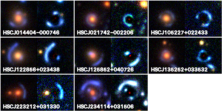
Figure 1: Grade A lens candidates. For each candidate, the left panel shows the composite $gri$ color image from the HSC SSP imaging, while the right panel shows the image with the lens galaxy subtracted by YattaLens. The cutouts are roughly $\sim 10\arcsec\times 10\arcsec$.

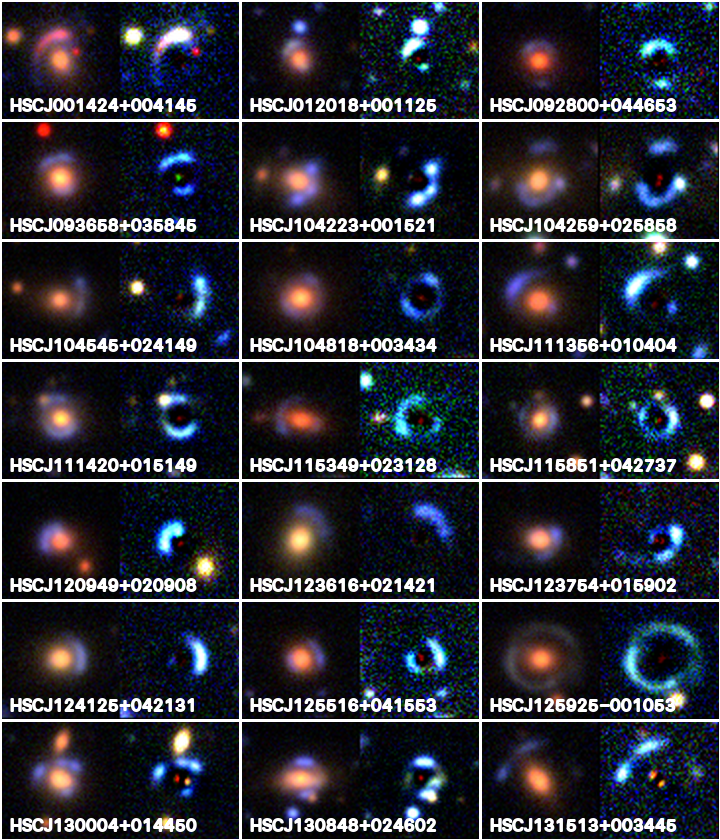
Figure 2: Grade B lens candidates, similar to Figure 1.

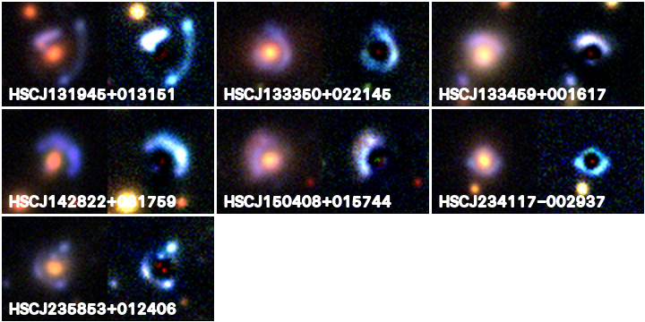
Figure 2: (Continued.)

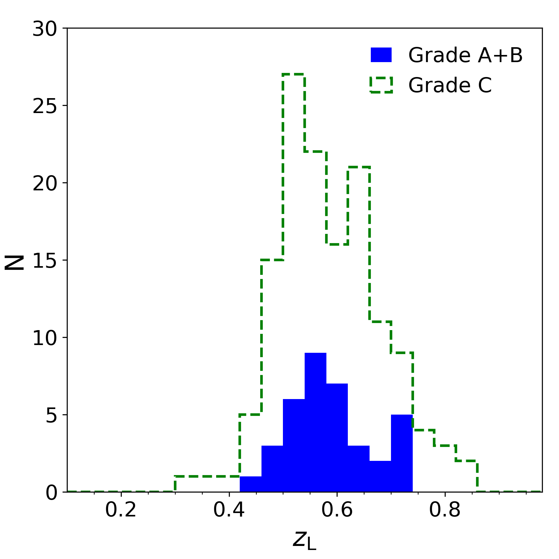
Figure 3: Histogram of spectroscopic lens redshifts for the lens candidates found in this study. The grade A and grade B candidates are combined (blue solid histogram) and shown separately from the grade C candidates (green dashed histogram).

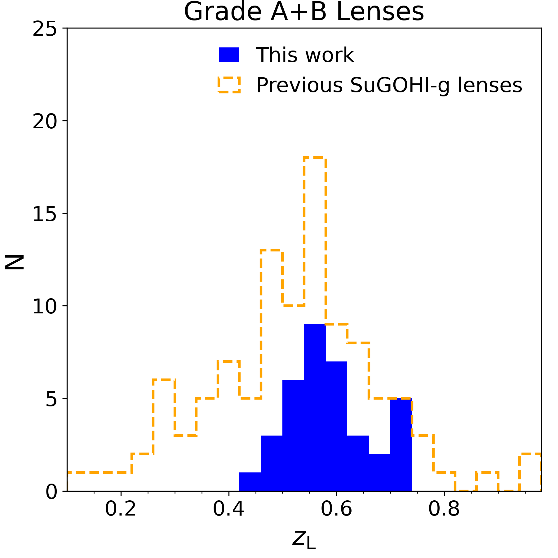
Figure 4: Histogram of spectroscopic lens redshifts for the 36 combined grade A and grade B lens candidates found in this study (blue solid histogram), compared to lens redshifts for the existing 106 grade A and grade B galaxy-galaxy lenses in the SuGOHI-g sample (orange dashed histogram) that have known lens redshifts.

4.1 Overlap with other lens searches

Separate from this work, Cañameras et al. (2021), Shu et al. (2022), and Jaelani et al. (in preparation) have recently applied machine learning-based lens search algorithms to the HSC SSP Public Data Release 2 (Aihara et al., 2019) and have published lens candidates from these searches. Additional lens candidates from recent lens searches in other surveys have also been compiled and are cross-matched with our candidates (R. Cañameras, private communication).

Although our work is based on a larger dataset, there is some overlap in the candidates we have discovered, and the quality of the HSC imaging data is often superior to those of these previous searches. We have indicated these candidates and cited the appropriate references in Table 1. While some of these previous searches graded the lens candidates in a similar way to this study, they are often based on lower-quality data or used a slightly different grading scheme. As such, we do not take into consideration a candidate’s grade or likelihood of being a lens from these previous studies.

4.2 Comparison to previous searches and datasets

We compare the statistics of lens candidates selected in this paper to previous searches in the HSC SSP using YattaLens. The Sonnenfeld et al. (2018) sample includes candidates selected through other methods, so it’s not quite a fair comparison to this work. Wong et al. (2018) used YattaLens to analyze $\sim 31000$ LRGs and identify 772 candidates, while this paper analyzes 103191 LRGs and returns 2319 candidates, which is a comparable rate. After inspection, Wong et al. (2018) finds 200 definite/probable/possible candidates out of 776, while this paper finds 174 such candidates out of 2319. This difference can be partially explained by our pre-selection, which removed $\sim 150$ known and previously-selected candidates from entire SuGOHI sample of galaxy-scale lenses. Had these systems not been filtered out, many of them likely would have been identified by YattaLens and graded as possible candidates. The lower rate in this paper may also be partially due to more conservative scoring, as was suggested in Section 4.1.

It is difficult to directly compare the number lens candidates found in various surveys due to different survey depths, image quality, and area, as well as differences in the criteria used to judge the quality of a lens candidate. Nevertheless, we can comment on a few comparable datasets and the size of the of lens candidate samples from them to the SuGOHI-g sample to give a broad overview of where our sample stands in relation to them. Restricting the sample to galaxy-galaxy lenses with a grade of either A, B, or C from SuGOHI publications (i.e., not including external publications such as Cañameras et al. (2021), Shu et al. (2022), etc.), we have identified 1464 lens candidates (of which 282 are grade A or B) to date in the HSC SSP in 1310 deg² through the latest data release. By comparison, a search for strong lenses in the Kilo-Degree Survey found 268 “high-quality" candidates (Petrillo et al., 2019; Li et al., 2020, 2021) in $\sim 1350$ deg². A search through $\sim 30000$ deg² in Pan-STARRS by Cañameras et al. (2020) found 353 candidates with a grade roughly equivalent to our grade A and B lenses. Finally, the survey most comparable to the HSC SSP is the Dark Energy Survey, in which lens searches through $\sim 5000$ deg² have yielded $\sim 500$ “probable" lenses and $\sim 750$ “possible" lenses (Jacobs et al., 2019), with an additional 186 candidates identified by Rojas et al. (2021). In this context, the HSC SSP is quite competitive in number of lens candidates identified relative to survey area. It should be noted again that the greater depth of the HSC SSP makes us more likely to detect fainter and higher-redshift lenses, which fills a valuable niche.

4.3 Comments on Individual Lens Candidates

Here, we briefly comment on a few notable systems among the grade A and B candidates that we have discovered.

4.3.1 Group-scale lenses

Some of our lens candidates are potentially group-scale lenses, as they either have multiple galaxies within the arc(s), or have an arc radius that implies a much larger lensing mass than a single lens galaxy. These systems are HSCJ104545+024149 (grade B), HSCJ131945+013151 (grade B), and HSCJ223212+031330 (grade A). These candidates, if confirmed, may be valuable for studying group-scale halos, particularly the distribution of the dark matter within these structures.

4.3.2 HSCJ234114+031506: A potential double source plane lens

Based on the image configuration, HSCJ234114+031506 (grade A) is a potential double source plane lens (DSPL), in which there are two distinct sources at different redshifts. These systems are valuable due to the improved constraints on the lens model and the potential to constrain cosmological parameters (e.g., Collett et al. (2012); Collett & Auger (2014); Linder (2016)), but are extremely rare. Only a handful of galaxy-scale DSPLs been discovered so far, including one spectroscopically-confirmed system from the HSC SSP (the “Eye of Horus"; Tanaka et al. (2016)).

The large northern arc in HSCJ234114+031506 is an obvious lensed feature, but it is unclear whether the compact image just south of the lens galaxy is the counterimage of this arc, or of the other nearby clump (northeast of the lens galaxy) interior to the arc. In addition, the more distant object to the west of the lens galaxy may be a counterimage of the northeast clump. Follow-up spectroscopy should reveal the nature of these objects.

5 Summary

As part of the SuGOHI project, we have conducted a search for galaxy-scale strong gravitational lenses in DR4 of the HSC SSP (covering 1310 deg² in the $grizy$ bands) using the lens-finding algorithm YattaLens. We run the search on 103191 LRGs with spectroscopy from BOSS DR15 and visually inspect and grade the candidates identified by YattaLens as potential lenses. We find 8 definite (grade A) lenses, 28 probable (grade B) lenses, and 138 possible (grade C) lenses. We cross-check with recent lens searches in the literature. The lens candidates have lens redshifts primarily in the range $0.3\lesssim z_{\mathrm{L}}\lesssim 0.9$, consistent with previous lenses found as part of SuGOHI-g. This intermediate redshift range makes this sample valuable for future studies of the evolution of galaxy structure from $z\sim 1$ to the present epoch. Follow-up spectroscopy will confirm these lenses and measure source redshifts to enable science results from detailed lens modeling.

We thank the referee, whose comments helped to improve this paper. We thank Alessandro Sonnenfeld, Sherry Suyu, and Masayuki Tanaka for useful discussions and input. We thank Raoul Cañameras and Yiping Shu for providing an updated list of lens candidates from recent searches with which to cross-check our newly discovered candidates. The Hyper Suprime-Cam (HSC) collaboration includes the astronomical communities of Japan and Taiwan, and Princeton University. The HSC instrumentation and software were developed by the National Astronomical Observatory of Japan (NAOJ), the Kavli Institute for the Physics and Mathematics of the Universe (Kavli IPMU), the University of Tokyo, the High Energy Accelerator Research Organization (KEK), the Academia Sinica Institute for Astronomy and Astrophysics in Taiwan (ASIAA), and Princeton University. Funding was contributed by the FIRST program from the Japanese Cabinet Office, the Ministry of Education, Culture, Sports, Science and Technology (MEXT), the Japan Society for the Promotion of Science (JSPS), Japan Science and Technology Agency (JST), the Toray Science Foundation, NAOJ, Kavli IPMU, KEK, ASIAA, and Princeton University. This paper is based in part on data collected at the Subaru Telescope and retrieved from the HSC data archive system, which is operated by Subaru Telescope and Astronomy Data Center (ADC) at NAOJ. Data analysis was in part carried out with the cooperation of Center for Computational Astrophysics (CfCA) at NAOJ. We are honored and grateful for the opportunity of observing the Universe from Maunakea, which has the cultural, historical and natural significance in Hawaii. This paper makes use of software developed for Vera C. Rubin Observatory. We thank the Rubin Observatory for making their code available as free software at http://pipelines.lsst.io/. Funding for SDSS-III has been provided by the Alfred P. Sloan Foundation, the Participating Institutions, the National Science Foundation, and the U.S. Department of Energy Office of Science. The SDSS-III web site is http://www.sdss3.org/. SDSS-III is managed by the Astrophysical Research Consortium for the Participating Institutions of the SDSS-III Collaboration including the University of Arizona, the Brazilian Participation Group, Brookhaven National Laboratory, Carnegie Mellon University, University of Florida, the French Participation Group, the German Participation Group, Harvard University, the Instituto de Astrofisica de Canarias, the Michigan State/Notre Dame/JINA Participation Group, Johns Hopkins University, Lawrence Berkeley National Laboratory, Max Planck Institute for Astrophysics, Max Planck Institute for Extraterrestrial Physics, New Mexico State University, New York University, Ohio State University, Pennsylvania State University, University of Portsmouth, Princeton University, the Spanish Participation Group, University of Tokyo, University of Utah, Vanderbilt University, University of Virginia, University of Washington, and Yale University. This work is supported by JSPS KAKENHI Grant Numbers JP20K14511, JP20K04016, JP20H00181, JP20H05856, and JP18K03693. J. H. H. C. acknowledges support from the Swiss National Science Foundation (SNSF). A. T. J. is supported by Riset ITB 2021. This research made use of Astropy, a community-developed core Python package for Astronomy (Astropy Collaboration et al., 2013, 2018). This research made use of Matplotlib, a 2D graphics package used for Python (Hunter, 2007).

Grade C Lens Candidates

For completeness, we list the grade C lens candidates identified in our lens search here in Table 2.

Table 2: Grade C Lens candidates

Name	$\alpha$ (J2000)	$\delta$ (J2000)	$z_{\mathrm{L}}$
HSCJ000106+010329	0.2771	1.0583	0.7213
HSCJ000158+043438	0.4928	4.5774	0.6753
HSCJ000222+042125	0.5957	4.3571	0.7072
HSCJ000449+041056	1.2048	4.1824	0.4934
HSCJ000733+022624	1.8898	2.4401	0.4647
HSCJ001144+010102	2.9359	1.0175	0.7936
HSCJ001317+020931	3.3243	2.1588	0.5432
HSCJ002037+002058	5.1575	0.3497	0.3288
HSCJ002624+041825	6.6039	4.3071	0.7169
HSCJ002652+030356	6.7171	3.0656	0.6469
HSCJ003254+004839	8.2257	0.8109	0.6573
HSCJ003632+014916	9.1363	1.8213	0.6477
HSCJ003650+005316	9.2112	0.8880	0.6029
HSCJ005356+015546	13.4848	1.9296	0.6891
HSCJ005453+022522	13.7214	2.4230	0.5046
HSCJ005630–001123	14.1279	-0.1900	0.6811
HSCJ005937+010731	14.9066	1.1255	0.6577
HSCJ010021–004349	15.0899	-0.7303	0.5548
HSCJ010201+025404	15.5067	2.9014	0.5581
HSCJ010434+035410	16.1452	3.9030	0.5438
HSCJ012308+011027	20.7850	1.1743	0.6541
HSCJ012411+025155	21.0477	2.8654	0.5084
HSCJ013539+025615	23.9146	2.9376	0.5772
HSCJ014101+032742	25.2573	3.4617	0.5218
HSCJ020745+004721	31.9391	0.7894	0.5422
HSCJ021214+002719	33.0617	0.4553	0.5372
HSCJ021803–000254	34.5159	-0.0486	0.3472
HSCJ022027–004453	35.1139	-0.7481	0.7743
HSCJ022314–002558	35.8110	-0.4328	0.5614
HSCJ022624–001716	36.6001	-0.2879	0.5540
HSCJ023637+025729	39.1560	2.9583	0.6683
HSCJ083759+050612	129.4976	5.1035	0.6284
HSCJ083841+025720	129.6733	2.9556	0.5408
HSCJ084306+051435	130.7774	5.2431	0.6232
HSCJ084905+034329	132.2738	3.7249	0.4659
HSCJ085247+045218	133.1982	4.8718	0.5458
HSCJ093626+034716	144.1122	3.7878	0.6962
HSCJ093844+015406	144.6855	1.9019	0.8345
HSCJ101734–001227	154.3919	-0.2076	0.8457
HSCJ102041+002226	155.1714	0.3739	0.6143

Lens redshifts are from SDSS DR15.

Table 2: (Continued.)

Name	$\alpha$ (J2000)	$\delta$ (J2000)	$z_{\mathrm{L}}$
HSCJ102117+031442	155.3225	3.2450	0.6742
HSCJ102311–000702	155.7989	-0.1174	0.4735
HSCJ102858–013141	157.2419	-1.5282	0.5178
HSCJ103430+042557	158.6265	4.4326	0.6546
HSCJ103519+050108	158.8324	5.0191	0.6353
HSCJ104146+021925	160.4429	2.3238	0.4850
HSCJ104307+041425	160.7815	4.2403	0.5751
HSCJ104358+022843	160.9950	2.4789	0.7851
HSCJ104549–002713	161.4574	-0.4538	0.5017
HSCJ104727+024906	161.8667	2.8184	0.5699
HSCJ104817+004336	162.0720	0.7268	0.5811
HSCJ105202+001427	163.0107	0.2409	0.6272
HSCJ105329+012255	163.3739	1.3820	0.7975
HSCJ105338+045536	163.4101	4.9267	0.5050
HSCJ105813+031136	164.5554	3.1934	0.4728
HSCJ110028+024436	165.1200	2.7436	0.5228
HSCJ110114+002016	165.3094	0.3380	0.6085
HSCJ110155+032954	165.4827	3.4985	0.4440
HSCJ110404–003703	166.0190	-0.6175	0.5027
HSCJ110511+042147	166.2978	4.3632	0.7176
HSCJ110840–001927	167.1686	-0.3244	0.4505
HSCJ110905+005118	167.2712	0.8551	0.6368
HSCJ111230+043153	168.1281	4.5314	0.4993
HSCJ111618+033628	169.0772	3.6079	0.4661
HSCJ111818+021102	169.5774	2.1840	0.5180
HSCJ112203–014707	170.5144	-1.7854	0.4525
HSCJ112221–011759	170.5890	-1.3000	0.7005
HSCJ112710+025956	171.7928	2.9991	0.5387
HSCJ113838+050110	174.6612	5.0196	0.6475
HSCJ114358+022513	175.9927	2.4205	0.6342
HSCJ114847+032706	177.1993	3.4518	0.6271
HSCJ115247+034254	178.1973	3.7152	0.5721
HSCJ115313+030814	178.3060	3.1373	0.5844
HSCJ115446+042415	178.6934	4.4042	0.7196
HSCJ115907+051911	179.7829	5.3200	0.4692
HSCJ120233+042541	180.6395	4.4281	0.5077
HSCJ120255+034044	180.7314	3.6791	0.5256
HSCJ120745+041400	181.9380	4.2334	0.6194
HSCJ121040+033354	182.6697	3.5652	0.7540
HSCJ122843+023818	187.1824	2.6385	0.5260

Table 2: (Continued.)

Name	$\alpha$ (J2000)	$\delta$ (J2000)	$z_{\mathrm{L}}$
HSCJ122948+013652	187.4527	1.6146	0.6183
HSCJ123035+052251	187.6474	5.3810	0.4701
HSCJ124503+024354	191.2632	2.7319	0.4949
HSCJ124629+004116	191.6211	0.6880	0.5730
HSCJ125220+025504	193.0858	2.9180	0.5178
HSCJ125604–003229	194.0177	-0.5415	0.7249
HSCJ125903+014542	194.7630	1.7618	0.5178
HSCJ130044+031657	195.1864	3.2826	0.6798
HSCJ130500+032545	196.2540	3.4293	0.5266
HSCJ131037+021947	197.6551	2.3300	0.5056
HSCJ131140+025539	197.9179	2.9276	0.6115
HSCJ131417–010555	198.5711	-1.0989	0.4833
HSCJ131519+040008	198.8315	4.0024	0.7557
HSCJ131604+040924	199.0194	4.1569	0.5786
HSCJ131626+020910	199.1089	2.1530	0.6845
HSCJ131759+025548	199.4975	2.9302	0.6018
HSCJ131933–004256	199.8885	-0.7158	0.6575
HSCJ132221–012821	200.5878	-1.4727	0.5423
HSCJ132439–015026	201.1664	-1.8407	0.4379
HSCJ132904+020015	202.2679	2.0044	0.5195
HSCJ133328+425215	203.3694	42.8711	0.5873
HSCJ134017+420751	205.0742	42.1311	0.5370
HSCJ134504–012202	206.2705	-1.3673	0.5555
HSCJ135110+443315	207.7926	44.5544	0.5650
HSCJ135346+021338	208.4447	2.2274	0.4589
HSCJ140218+022318	210.5786	2.3884	0.6941
HSCJ140252+023101	210.7177	2.5171	0.6017
HSCJ140347+425700	210.9459	42.9503	0.3946
HSCJ141628+030004	214.1204	3.0013	0.4899
HSCJ141758+022347	214.4942	2.3965	0.5219
HSCJ142240+441140	215.6670	44.1946	0.5859
HSCJ142532+032850	216.3843	3.4806	0.5294
HSCJ142615+033050	216.5661	3.5139	0.5237
HSCJ142652+433113	216.7175	43.5204	0.5770
HSCJ142820+031902	217.0869	3.3175	0.5933
HSCJ143018+034441	217.5776	3.7448	0.6769
HSCJ144411+030655	221.0478	3.1153	0.7677
HSCJ144530+434129	221.3752	43.6915	0.5332
HSCJ145130+042054	222.8785	4.3484	0.7004
HSCJ220958+013722	332.4942	1.6230	0.6250

Table 2: (Continued.)

Name	$\alpha$ (J2000)	$\delta$ (J2000)	$z_{\mathrm{L}}$
HSCJ221655+035733	334.2325	3.9594	0.5469
HSCJ222653+035502	336.7215	3.9173	0.6978
HSCJ222951–012440	337.4645	-1.4111	0.7065
HSCJ223315+041108	338.3137	4.1858	0.6318
HSCJ223513+034313	338.8063	3.7204	0.6316
HSCJ224101+041820	340.2567	4.3056	0.5916
HSCJ231207+043501	348.0295	4.5839	0.5597
HSCJ231740+040317	349.4181	4.0548	0.5851
HSCJ232546–003916	351.4424	-0.6547	0.6010
HSCJ232833+024214	352.1385	2.7040	0.4926
HSCJ233219+022838	353.0827	2.4772	0.6517
HSCJ233917+010908	354.8243	1.1523	0.6262
HSCJ233945+015726	354.9379	1.9575	0.5046
HSCJ234246+044345	355.6932	4.7292	0.4915
HSCJ234824+025357	357.1015	2.8993	0.5498
HSCJ235052+035356	357.7167	3.8990	0.5145
HSCJ235503+014443	358.7653	1.7453	0.5224
HSCJ235730+010133	359.3776	1.0260	0.6379

References

- Aguado et al. (2019) Aguado, D. S., et al. 2019, ApJS, 240, 23
- Aihara et al. (2018) Aihara, H., et al. 2018, PASJ, 70, S4
- Aihara et al. (2019) —. 2019, PASJ, 71, 114
- Astropy Collaboration et al. (2013) Astropy Collaboration, et al. 2013, A&A, 558, A33
- Astropy Collaboration et al. (2018) —. 2018, AJ, 156, 123
- Auger et al. (2010) Auger, M. W., Treu, T., Bolton, A. S., Gavazzi, R., Koopmans, L. V. E., Marshall, P. J., Moustakas, L. A., & Burles, S. 2010, ApJ, 724, 511
- Auger et al. (2011) Auger, M. W., Treu, T., Brewer, B. J., & Marshall, P. J. 2011, MNRAS, 411, L6
- Bertin & Arnouts (1996) Bertin, E., & Arnouts, S. 1996, A&AS, 117, 393
- Birrer et al. (2020) Birrer, S., et al. 2020, A&A, 643, A165
- Bosch et al. (2018) Bosch, J., et al. 2018, PASJ, 70, S5
- Cañameras et al. (2020) Cañameras, R., et al. 2020, A&A, 644, A163
- Cañameras et al. (2021) —. 2021, A&A, 653, L6
- Cao et al. (2020) Cao, X., Li, R., Shu, Y., Mao, S., Kneib, J.-P., & Gao, L. 2020, MNRAS, 499, 3610
- Chan et al. (2020) Chan, J. H. H., et al. 2020, A&A, 636, A87
- Collett & Auger (2014) Collett, T. E., & Auger, M. W. 2014, MNRAS, 443, 969
- Collett et al. (2012) Collett, T. E., Auger, M. W., Belokurov, V., Marshall, P. J., & Hall, A. C. 2012, MNRAS, 424, 2864
- Dawson et al. (2013) Dawson, K. S., et al. 2013, AJ, 145, 10
- de Vaucouleurs (1948) de Vaucouleurs, G. 1948, Annales d’Astrophysique, 11, 247
- Drinkwater et al. (2017) Drinkwater, M. J., et al. 2017, Monthly Notices of the Royal Astronomical Society, 474, 4151. https://doi.org/10.1093/mnras/stx2963
- Eisenstein et al. (2011) Eisenstein, D. J., et al. 2011, AJ, 142, 72
- Gilman et al. (2020) Gilman, D., Birrer, S., Nierenberg, A., Treu, T., Du, X., & Benson, A. 2020, MNRAS, 491, 6077
- Huang et al. (2021) Huang, X., et al. 2021, ApJ, 909, 27
- Hunter (2007) Hunter, J. D. 2007, Computing in Science & Engineering, 9, 90
- Jacobs et al. (2019) Jacobs, C., et al. 2019, ApJS, 243, 17
- Jaelani et al. (2020) Jaelani, A. T., et al. 2020, MNRAS, 495, 1291
- Kawanomoto et al. (2018) Kawanomoto, S., et al. 2018, Publications of the Astronomical Society of Japan, psy056. http://dx.doi.org/10.1093/pasj/psy056
- Komiyama et al. (2018) Komiyama, Y., et al. 2018, PASJ, 70, S2
- Koopmans et al. (2006) Koopmans, L. V. E., Treu, T., Bolton, A. S., Burles, S., & Moustakas, L. A. 2006, ApJ, 649, 599
- Koopmans et al. (2009) Koopmans, L. V. E., et al. 2009, ApJ, 703, L51
- Li et al. (2020) Li, R., et al. 2020, ApJ, 899, 30
- Li et al. (2021) —. 2021, ApJ, 923, 16
- Linder (2016) Linder, E. V. 2016, Phys. Rev. D, 94, 083510
- Miyazaki et al. (2012) Miyazaki, S., et al. 2012, in Proc. SPIE, Vol. 8446, Ground-based and Airborne Instrumentation for Astronomy IV, 84460Z
- Miyazaki et al. (2018) Miyazaki, S., et al. 2018, PASJ, 70, S1
- Nierenberg et al. (2014) Nierenberg, A. M., Treu, T., Wright, S. A., Fassnacht, C. D., & Auger, M. W. 2014, MNRAS, 442, 2434
- Nierenberg et al. (2017) Nierenberg, A. M., et al. 2017, MNRAS, 471, 2224
- Petrillo et al. (2019) Petrillo, C. E., et al. 2019, MNRAS, 484, 3879
- Refsdal (1964) Refsdal, S. 1964, MNRAS, 128, 307
- Rojas et al. (2021) Rojas, K., et al. 2021, arXiv e-prints, arXiv:2109.00014
- Shu et al. (2022) Shu, Y., Cañameras, R., Schuldt, S., Suyu, S. H., Taubenberger, S., Inoue, K. T., & Jaelani, A. T. 2022, A&A, 662, A4
- Sonnenfeld et al. (2019) Sonnenfeld, A., Jaelani, A. T., Chan, J., More, A., Suyu, S. H., Wong, K. C., Oguri, M., & Lee, C.-H. 2019, A&A, 630, A71
- Sonnenfeld et al. (2018) Sonnenfeld, A., et al. 2018, PASJ, 70, S29
- Sonnenfeld et al. (2020) —. 2020, A&A, 642, A148
- Stein et al. (2022) Stein, G., Blaum, J., Harrington, P., Medan, T., & Lukić, Z. 2022, ApJ, 932, 107
- Talbot et al. (2021) Talbot, M. S., Brownstein, J. R., Dawson, K. S., Kneib, J.-P., & Bautista, J. 2021, MNRAS, 502, 4617
- Tanaka et al. (2016) Tanaka, M., et al. 2016, ApJ, 826, L19
- Treu et al. (2010) Treu, T., Auger, M. W., Koopmans, L. V. E., Gavazzi, R., Marshall, P. J., & Bolton, A. S. 2010, ApJ, 709, 1195
- Vegetti et al. (2014) Vegetti, S., Koopmans, L. V. E., Auger, M. W., Treu, T., & Bolton, A. S. 2014, MNRAS, 442, 2017
- Vegetti et al. (2010) Vegetti, S., Koopmans, L. V. E., Bolton, A., Treu, T., & Gavazzi, R. 2010, MNRAS, 408, 1969
- Vegetti et al. (2012) Vegetti, S., Lagattuta, D. J., McKean, J. P., Auger, M. W., Fassnacht, C. D., & Koopmans, L. V. E. 2012, Nature, 481, 341
- Wong et al. (2018) Wong, K. C., et al. 2018, ApJ, 867, 107
- Wong et al. (2020) —. 2020, MNRAS, 498, 1420