DPar2: Fast and Scalable PARAFAC2 Decomposition for Irregular Dense Tensors

Abstract

Given an irregular dense tensor, how can we efficiently analyze it? An irregular tensor is a collection of matrices whose columns have the same size and rows have different sizes from each other. PARAFAC2 decomposition is a fundamental tool to deal with an irregular tensor in applications including phenotype discovery and trend analysis. Although several PARAFAC2 decomposition methods exist, their efficiency is limited for irregular dense tensors due to the expensive computations involved with the tensor.

In this paper, we propose DPar2, a fast and scalable PARAFAC2 decomposition method for irregular dense tensors. DPar2 achieves high efficiency by effectively compressing each slice matrix of a given irregular tensor, careful reordering of computations with the compression results, and exploiting the irregularity of the tensor. Extensive experiments show that DPar2 is up to $6.0\times$ faster than competitors on real-world irregular tensors while achieving comparable accuracy. In addition, DPar2 is scalable with respect to the tensor size and target rank.

I Introduction

How can we efficiently analyze an irregular dense tensor? Many real-world multi-dimensional arrays are represented as irregular dense tensors; an irregular tensor is a collection of matrices with different row lengths. For example, stock data can be represented as an irregular dense tensor; the listing period is different for each stock (irregularity), and almost all of the entries of the tensor are observable during the listing period (high density). The irregular tensor of stock data is the collection of the stock matrices whose row and column dimension corresponds to time and features (e.g., the opening price, the closing price, the trade volume, etc.), respectively. In addition to stock data, many real-world data including music song data and sound data are also represented as irregular dense tensors. Each song can be represented as a slice matrix (e.g., time-by-frequency matrix) whose rows correspond to the time dimension. Then, the collection of songs is represented as an irregular tensor consisting of slice matrices of songs each of whose time length is different. Sound data are represented similarly.

Tensor decomposition has attracted much attention from the data mining community to analyze tensors [1, 2, 3, 4, 5, 6, 7, 8, 9, 10]. Specifically, PARAFAC2 decomposition has been widely used for modeling irregular tensors in various applications including phenotype discovery [11, 12], trend analysis [13], and fault detection [14]. However, existing PARAFAC2 decomposition methods are not fast and scalable enough for irregular dense tensors. Perros et al. [11] improve the efficiency for handling irregular sparse tensors, by exploiting the sparsity patterns of a given irregular tensor. Many recent works [12, 15, 16, 17] adopt their idea to handle irregular sparse tensors. However, they are not applicable to irregular dense tensors that have no sparsity pattern. Although Cheng and Haardt [18] improve the efficiency of PARAFAC2 decomposition by preprocessing a given tensor, there is plenty of room for improvement in terms of computational costs. Moreover, there remains a need for fully employing multicore parallelism. The main challenge to successfully design a fast and scalable PARAFAC2 decomposition method is how to minimize the computational costs involved with an irregular dense tensor and the intermediate data generated in updating factor matrices.

In this paper, we propose DPar2 (Dense PARAFAC2 decomposition), a fast and scalable PARAFAC2 decomposition method for irregular dense tensors. Based on the characteristics of real-world data, DPar2 compresses each slice matrix of a given irregular tensor using randomized Singular Value Decomposition (SVD). The small compressed results and our careful ordering of computations considerably reduce the computational costs and the intermediate data. In addition, DPar2 maximizes multi-core parallelism by considering the difference in sizes between slices. With these ideas, DPar2 achieves higher efficiency and scalability than existing PARAFAC2 decomposition methods on irregular dense tensors. Extensive experiments show that DPar2 outperforms the existing methods in terms of speed, space, and scalability, while achieving a comparable fitness, where the fitness indicates how a method approximates a given data well (see Section IV-A).

(a) Trade-off

(b) Trade-off

(c) Trade-off

(d) Trade-off

Figure 1: [Best viewed in color] Measurement of the running time and fitness on real-world datasets for three target ranks $R$: $10$, $15$, and $20$. DPar2 provides the best trade-off between speed and fitness. DPar2 is up to $6.0\times$ faster than the competitors while having a comparable fitness.

The contributions of this paper are as follows.

Algorithm. We propose DPar2, a fast and scalable PARAFAC2 decomposition method for decomposing irregular dense tensors.

Analysis. We provide analysis for the time and the space complexities of our proposed method DPar2.

Experiment. DPar2 achieves up to $6.0\times$ faster running time than previous PARAFAC2 decomposition methods based on ALS while achieving a similar fitness (see Fig. 1).

Discovery. With DPar2, we find that the Korean stock market and the US stock market have different correlations (see Fig. 12) between features (e.g., prices and technical indicators). We also find similar stocks (see Table III) on the US stock market during a specific event (e.g., COVID-19).

In the rest of this paper, we describe the preliminaries in Section II, propose our method DPar2 in Section III, present experimental results in Section IV, discuss related works in Section V, and conclude in Section VI. The code and datasets are available at https://datalab.snu.ac.kr/dpar2.

II Preliminaries

In this section, we describe tensor notations, tensor operations, Singular Value Decomposition (SVD), and PARAFAC2 decomposition. We use the symbols listed in Table I.

TABLE I: Symbol description.

Symbol	Description
$\{\mathbf{X}_{k}\}^{K}_{k=1}$	irregular tensor of slices $\mathbf{X}_{k}$ for $k=1,...,K$
$\mathbf{X}_{k}$	slice matrix ($\in I_{k}\times J$)
$\mathbf{X}(i,:)$	$i$-th row of a matrix $\mathbf{X}$
$\mathbf{X}(:,j)$	$j$-th column of a matrix $\mathbf{X}$
$\mathbf{X}(i,j)$	$(i,j)$-th element of a matrix $\mathbf{X}$
$\mathbf{X}_{(n)}$	mode-$n$ matricization of a tensor $\boldsymbol{\mathscr{X}}$
$\mathbf{Q}_{k}$, $\mathbf{S}_{k}$	factor matrices of the $k$th slice
$\mathbf{H}$, $\mathbf{V}$	factor matrices of an irregular tensor
$\mathbf{A}_{k}$, $\mathbf{B}_{k}$, $\mathbf{C}_{k}$	SVD results of the $k$th slice
$\mathbf{D}$, $\mathbf{E}$, $\mathbf{F}$	SVD results of the second stage
$\mathbf{F}^{(k)}$	$k$th vertical block matrix $(\in\mathbb{R}^{R\times R})$ of $\mathbf{F}(\in\mathbb{R}^{KR\times R})$
$\mathbf{Z}_{k}$, $\mathbf{\Sigma_{k}}$, $\mathbf{P}_{k}$	SVD results of $\mathbf{F}^{(k)}\mathbf{E}\mathbf{D}^{T}\mathbf{V}\mathbf{S}_{k}\mathbf{H}^{T}$
$R$	target rank
$\otimes$	Kronecker product
$\odot$	Khatri-Rao product
$*$	element-wise product
$\mathbin{\|}$	horizontal concatenation
$vec(\cdot)$	vectorization of a matrix

II-A Tensor Notation and Operation

We use boldface lowercases (e.g. $\mathbf{x}$) and boldface capitals (e.g. $\mathbf{X}$) for vectors and matrices, respectively. In this paper, indices start at $1$. An irregular tensor is a 3-order tensor $\boldsymbol{\mathscr{X}}$ whose $k$-frontal slice $\boldsymbol{\mathscr{X}}(:,:,k)$ is $\mathbf{X}_{k}\in\mathbb{R}^{I_{k}\times J}$. We denote irregular tensors by $\{\mathbf{X}_{k}\}^{K}_{k=1}$ instead of $\boldsymbol{\mathscr{X}}$ where $K$ is the number of $k$-frontal slices of the tensor. An example is described in Fig. 2. We refer the reader to [19] for the definitions of tensor operations including Frobenius norm, matricization, Kronecker product, and Khatri-Rao product.

II-B Singular Value Decomposition (SVD)

Singular Value Decomposition (SVD) decomposes $\mathbf{A}\in\mathbb{R}^{I\times J}$ to $\mathbf{X}=\mathbf{U}\mathbf{\Sigma}\mathbf{V}^{\text{T}}$. $\mathbf{U}\in\mathbb{R}^{I\times R}$ is the left singular vector matrix of $\mathbf{A}$; $\mathbf{U}=\begin{bmatrix}\mathbf{u}_{1}\cdots\mathbf{u}_{r}\end{bmatrix}$ is a column orthogonal matrix where $R$ is the rank of $\mathbf{A}$ and $\mathbf{u}_{1}$, $\cdots$, $\mathbf{u}_{R}$ are the eigenvectors of $\mathbf{A}\mathbf{A}^{\text{T}}$. $\mathbf{\Sigma}$ is an $R\times R$ diagonal matrix whose diagonal entries are singular values. The $i$-th singular value $\sigma_{i}$ is in $\mathbf{\Sigma}_{i,i}$ where $\sigma_{1}$ $\geq$ $\sigma_{2}$ $\geq$ $\cdots$ $\geq$ $\sigma_{R}$ $\geq$ $0$. $\mathbf{V}\in\mathbb{R}^{J\times R}$ is the right singular vector matrix of $\mathbf{A}$; $\mathbf{V}=\begin{bmatrix}\mathbf{v}_{1}\cdots\mathbf{v}_{R}\end{bmatrix}$ is a column orthogonal matrix where $\mathbf{v}_{1}$, $\cdots$, $\mathbf{v}_{R}$ are the eigenvectors of $\mathbf{A}^{\text{T}}\mathbf{A}$.

1

0:  $\mathbf{A}\in\mathbb{R}^{I\times J}$

0:  $\mathbf{U}\in\mathbb{R}^{I\times R}$, $\mathbf{S}\in\mathbb{R}^{R\times R}$, and $\mathbf{V}\in\mathbb{R}^{J\times R}$.

20:  target rank $R$, and an exponent $q$

1:  generate a Gaussian test matrix $\mathbf{\Omega}\in\mathbb{R}^{J\times(R+s)}$

2:  construct $\mathbf{Y}\leftarrow(\mathbf{A}\mathbf{A}^{T})^{q}\mathbf{A}\mathbf{\Omega}$

3:  $\mathbf{Q}\mathbf{R}\leftarrow\mathbf{Y}$ using QR factorization

4:  construct $\mathbf{B}\leftarrow\mathbf{Q}^{T}\mathbf{A}$

5:  $\tilde{\mathbf{U}}\mathbf{\Sigma}\mathbf{V}^{T}\leftarrow\mathbf{B}$ using truncated SVD at rank $R$

6:  return  $\mathbf{U}=\mathbf{Q}\tilde{\mathbf{U}}$, $\mathbf{\Sigma}$, and $\mathbf{V}$

Algorithm 1 Randomized SVD [20]

Randomized SVD. Many works [21, 20, 22] have introduced efficient SVD methods to decompose a matrix $\mathbf{A}\in\mathbb{R}^{I\times J}$ by applying randomized algorithms. We introduce a popular randomized SVD in Algorithm 1. Randomized SVD finds a column orthogonal matrix $\mathbf{Q}\in\mathbb{R}^{I\times(R+s)}$ of $(\mathbf{A}\mathbf{A}^{T})^{q}\mathbf{A}\mathbf{\Omega}$ using random matrix $\mathbf{\Omega}$, constructs a smaller matrix $\mathbf{B}=\mathbf{Q}^{T}\mathbf{A}$ $(\in\mathbb{R}^{(R+s)\times J})$, and finally obtains the SVD result $\mathbf{U}$ $(=\mathbf{Q}\tilde{\mathbf{U}})$, $\mathbf{\Sigma}$, $\mathbf{V}$ of $\mathbf{A}$ by computing SVD for $\mathbf{B}$, i.e., $\mathbf{B}\approx\tilde{\mathbf{U}}\mathbf{\Sigma}\mathbf{V}^{T}$. Given a matrix $\mathbf{A}$, the time complexity of randomized SVD is $\boldsymbol{\mathscr{O}}(IJR)$ where $R$ is the target rank.

II-C PARAFAC2 decomposition

PARAFAC2 decomposition proposed by Harshman [23] successfully deals with irregular tensors. The definition of PARAFAC2 decomposition is as follows:

Definition 1 (PARAFAC2 Decomposition).

Given a target rank $R$ and a 3-order tensor $\{\mathbf{X}_{k}\}^{K}_{k=1}$ whose $k$-frontal slice is $\mathbf{X}_{k}\in\mathbb{R}^{I_{k}\times J}$ for $k=1,...,K$, PARAFAC2 decomposition approximates each $k$-th frontal slice $\mathbf{X}_{k}$ by $\mathbf{U}_{k}\mathbf{S}_{k}\mathbf{V}^{T}$. $\mathbf{U}_{k}$ is a matrix of the size $I_{k}\times R$, $\mathbf{S}_{k}$ is a diagonal matrix of the size $R\times R$, and $\mathbf{V}$ is a matrix of the size $J\times R$ which are common for all the slices. $\Box$

1

0:  $\mathbf{X}_{k}\in\mathbb{R}^{I_{k}\times J}$ for $k=1,...,K$

0:  $\mathbf{U}_{k}\in\mathbb{R}^{I_{k}\times R}$, $\mathbf{S}_{k}\in\mathbb{R}^{R\times R}$ for $k=1,...,K$, and $\mathbf{V}\in\mathbb{R}^{J\times R}$.

20:  target rank $R$

1:  initialize matrices $\mathbf{H}\in\mathbb{R}^{R\times R}$, $\mathbf{V}$, and $\mathbf{S}_{k}$ for $k=1,...,K$

2:  repeat

3:     for $k=1,...,K$ do

34:        compute $\mathbf{Z}^{\prime}_{k}\mathbf{\Sigma^{\prime}_{k}}\mathbf{P}_{k}^{{}^{\prime}T}\leftarrow\mathbf{X}_{k}\mathbf{V}\mathbf{S}_{k}\mathbf{H}^{T}$ by performing truncated SVD at rank $R$

45:        $\mathbf{Q}_{k}\leftarrow\mathbf{Z}^{\prime}_{k}\mathbf{P}_{k}^{{}^{\prime}T}$

6:     end for

7:     for $k=1,...,K$ do

58:        $\mathbf{Y}_{k}\leftarrow\mathbf{Q}_{k}^{T}\mathbf{X}_{k}$

9:     end for

610:     construct a tensor $\boldsymbol{\mathscr{Y}}\in\mathbb{R}^{R\times J\times K}$ from slices $\mathbf{Y}_{k}\in\mathbb{R}^{R\times J}$ for $k=1,...,K$

/* running a single iteration of CP-ALS on $\boldsymbol{\mathscr{Y}}$ */

711:     $\mathbf{H}\leftarrow\mathbf{Y}_{(1)}(\mathbf{W}\odot\mathbf{V})(\mathbf{W}^{T}\mathbf{W}*\mathbf{V}^{T}\mathbf{V})^{\dagger}$

812:     $\mathbf{V}\leftarrow\mathbf{Y}_{(2)}(\mathbf{W}\odot\mathbf{H})(\mathbf{W}^{T}\mathbf{W}*\mathbf{H}^{T}\mathbf{H})^{\dagger}$

913:     $\mathbf{W}\leftarrow\mathbf{Y}_{(3)}(\mathbf{V}\odot\mathbf{H})(\mathbf{V}^{T}\mathbf{V}*\mathbf{H}^{T}\mathbf{H})^{\dagger}$

14:     for $k=1,...,K$ do

15:        $\mathbf{S}_{k}\leftarrow diag(\mathbf{W}(k,:))$

1016:     end for

1117:  until the maximum iteration is reached, or the error ceases to decrease;

18:  for $k=1,...,K$ do

19:     $\mathbf{U}_{k}\leftarrow\mathbf{Q}_{k}\mathbf{H}$

20:  end for

Algorithm 2 PARAFAC2-ALS [24]

The objective function of PARAFAC2 decomposition [23] is given as follows.

$$\min_{\{\mathbf{U}_{k}\},\{\mathbf{S}_{k}\},\mathbf{V}}\sum_{k=1}^{K}{||\mathbf{X}_{k}-\mathbf{U}_{k}\mathbf{S}_{k}\mathbf{V}^{T}||_{F}^{2}}$$ (1)

For uniqueness, Harshman [23] imposed the constraint (i.e., $\mathbf{U}_{k}^{T}\mathbf{U}=\Phi$ for all $k$), and replace $\mathbf{U}_{k}^{T}$ with $\mathbf{Q}_{k}\mathbf{H}$ where $\mathbf{Q}_{k}$ is a column orthogonal matrix and $\mathbf{H}$ is a common matrix for all the slices. Then, Equation (1) is reformulated with $\mathbf{Q}_{k}\mathbf{H}$:

$$\min_{\{\mathbf{Q}_{k}\},\{\mathbf{S}_{k}\},\mathbf{H},\mathbf{V}}\sum_{k=1}^{K}{||\mathbf{X}_{k}-\mathbf{Q}_{k}\mathbf{H}\mathbf{S}_{k}\mathbf{V}^{T}||_{F}^{2}}$$ (2)

Fig. 2 shows an example of PARAFAC2 decomposition for a given irregular tensor. A common approach to solve the above problem is ALS (Alternating Least Square) which iteratively updates a target factor matrix while fixing all factor matrices except for the target. Algorithm 2 describes PARAFAC2-ALS. First, we update each $\mathbf{Q}_{k}$ while fixing $\mathbf{H}$, $\mathbf{V}$, $\mathbf{S}_{k}$ for $k=1,...,K$ (lines 4 and 5). By computing SVD of $\mathbf{X}_{k}\mathbf{V}\mathbf{S}_{k}\mathbf{H}^{T}$ as $\mathbf{Z}^{\prime}_{k}\mathbf{\Sigma^{\prime}}_{k}\mathbf{P}_{k}^{{}^{\prime}T}$, we update $\mathbf{Q}_{k}$ as $\mathbf{Z}^{\prime}_{k}\mathbf{P}_{k}^{{}^{\prime}T}$, which minimizes Equation (3) over $\mathbf{Q}_{k}$ [11, 24, 25]. After updating $\mathbf{Q}_{k}$, the remaining factor matrices $\mathbf{H}$, $\mathbf{V}$, $\mathbf{S}_{k}$ is updated by minimizing the following objective function:

$$\min_{\{\mathbf{S}_{k}\},\mathbf{H},\mathbf{V}}\sum_{k=1}^{K}{||\mathbf{Q}_{k}^{T}\mathbf{X}_{k}-\mathbf{H}\mathbf{S}_{k}\mathbf{V}^{T}||_{F}^{2}}$$ (3)

Minimizing this function is to update $\mathbf{H}$, $\mathbf{V}$, $\mathbf{S}_{k}$ using CP decomposition of a tensor $\boldsymbol{\mathscr{Y}}\in\mathbb{R}^{R\times J\times K}$ whose $k$-th frontal slice is $\mathbf{Q}_{k}^{T}\mathbf{X}_{k}$ (lines 8 and 10). We run a single iteration of CP decomposition for updating them [24] (lines 11 to 16). $\mathbf{Q}_{k}$, $\mathbf{H}$, $\mathbf{S}_{k}$, and $\mathbf{V}$ are alternatively updated until convergence.

Iterative computations with an irregular dense tensor require high computational costs and large intermediate data. RD-ALS [18] reduces the costs by preprocessing a given tensor and performing PARAFAC2 decomposition using the preprocessed result, but the improvement of RD-ALS is limited. Also, recent works successfully have dealt with sparse irregular tensors by exploiting sparsity. However, the efficiency of their models depends on the sparsity patterns of a given irregular tensor, and thus there is little improvement on irregular dense tensors. Specifically, computations with large dense slices $\mathbf{X}_{k}$ for each iteration are burdensome as the number of iterations increases. We focus on improving the efficiency and scalability in irregular dense tensors.

III Proposed Method

In this section, we propose DPar2, a fast and scalable PARAFAC2 decomposition method for irregular dense tensors.

III-A Overview

Before describing main ideas of our method, we present main challenges that need to be tackled.

• Dealing with large irregular tensors. PARAFAC2 decomposition (Algorithm 2) iteratively updates factor matrices (i.e., $\mathbf{U}_{k}$, $\mathbf{S}_{k}$, and $\mathbf{V}$) using an input tensor. Dealing with a large input tensor is burdensome to update the factor matrices as the number of iterations increases.

• Minimizing numerical computations and intermediate data. How can we minimize the intermediate data and overall computations?

• Maximizing multi-core parallelism. How can we parallelize the computations for PARAFAC2 decomposition?

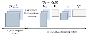
Figure 2: Example of PARAFAC2 decomposition. Given an irregular tensor $\{\mathbf{X}_{k}\}^{K}_{k=1}$, PARAFAC2 decomposes it into the factor matrices $\mathbf{H}$, $\mathbf{V}$, $\mathbf{Q}_{k}$, and $\mathbf{S}_{k}$ for $k=1,...,K$. Note that $\mathbf{Q}_{k}\mathbf{H}$ is equal to $\mathbf{U}_{k}$.

The main ideas that address the challenges mentioned above are as follows:

• Compressing an input tensor using randomized SVD considerably reduces the computational costs to update factor matrices (Section III-B).

• Careful reordering of computations with the compression results minimizes the intermediate data and the number of operations (Sections III-C to III-E).

• Careful distribution of work between threads enables DPar2 to achieve high efficiency by considering various lengths $I_{k}$ for $k=1,...,K$ (Section III-F).

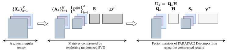
Figure 3: Overview of DPar2. Given an irregular tensor $\{\mathbf{X}_{k}\}^{K}_{k=1}$, DPar2 first compresses the given irregular tensor by exploiting randomized SVD. Then, DPar2 iteratively and efficiently updates the factor matrices, $\mathbf{Q}_{k}$, $\mathbf{H}$, $\mathbf{S}_{k}$, and $\mathbf{V}$, using only the compressed matrices, to get the result of PARAFAC2 decomposition.

As shown in Fig. 3, DPar2 first compresses each slice of an irregular tensor using randomized SVD (Section III-B). The compression is performed once before iterations, and only the compression results are used at iterations. It significantly reduces the time and space costs in updating factor matrices. After compression, DPar2 updates factor matrices at each iteration, by exploiting the compression results (Sections III-C to III-E). Careful reordering of computations is required to achieve high efficiency. Also, by carefully allocating input slices to threads, DPar2 accelerates the overall process (Section III-F).

III-B Compressing an irregular input tensor

DPar2 (see Algorithm 3) is a fast and scalable PARAFAC2 decomposition method based on ALS described in Algorithm 2. The main challenge that needs to be tackled is to minimize the number of heavy computations involved with a given irregular tensor $\{\mathbf{X}_{k}\}^{K}_{k=1}$ consisting of slices $\mathbf{X}_{k}$ for $k=1,...,K$ (in lines 4 and 8 of Algorithm 2). As the number of iterations increases (lines 2 to 17 in Algorithm 2), the heavy computations make PARAFAC2-ALS slow. For efficiency, we preprocess a given irregular tensor into small matrices, and then update factor matrices by carefully using the small ones.

Our approach to address the above challenges is to compress a given irregular tensor $\{\mathbf{X}_{k}\}^{K}_{k=1}$ before starting iterations. As shown in Fig. 4, our main idea is two-stage lossy compression with randomized SVD for the given tensor: 1) DPar2 performs randomized SVD for each slice $\mathbf{X}_{k}$ for $k=1,...,K$ at target rank $R$, and 2) DPar2 performs randomized SVD for a matrix, the horizontal concatenation of singular value matrices and right singular vector matrices of slices $\mathbf{X}_{k}$. Randomized SVD allows us to compress slice matrices with low computational costs and low errors.

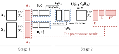
Figure 4: Two-stage SVD for a given irregular tensor. In the first stage, DPar2 performs randomized SVD of $\mathbf{X}_{k}$ for all $k$. In the second stage, DPar2 performs randomized SVD of $\mathbf{M}\in\mathbb{R}^{J\times KR}$ which is the horizontal concatenation of $\mathbf{C}_{k}\mathbf{B}_{k}$.

First Stage. In the first stage, DPar2 compresses a given irregular tensor by performing randomized SVD for each slice $\mathbf{X}_{k}$ at target rank $R$ (line 3 in Algorithm 3).

$$\mathbf{X}_{k}\approx\mathbf{A}_{k}\mathbf{B}_{k}\mathbf{C}_{k}^{T}$$ (4)

where $\mathbf{A}_{k}\in\mathbb{R}^{I_{k}\times R}$ is a matrix consisting of left singular vectors, $\mathbf{B}_{k}\in\mathbb{R}^{R\times R}$ is a diagonal matrix whose elements are singular values, and $\mathbf{C}_{k}\in\mathbb{R}^{J\times R}$ is a matrix consisting of right singular vectors.

Second Stage. Although small compressed data are generated in the first step, there is a room to further compress the intermediate data from the first stage. In the second stage, we compress a matrix $\mathbf{M}=\mathbin{\|}_{k=1}^{K}{\left(\mathbf{C}_{k}\mathbf{B}_{k}\right)}$ which is the horizontal concatenation of $\mathbf{C}_{k}\mathbf{B}_{k}$ for $k=1,...,K$. Compressing the matrix $\mathbf{M}$ maximizes the efficiency of updating factor matrices $\mathbf{H}$, $\mathbf{V}$, and $\mathbf{W}$ (see Equation (3)) at later iterations. We construct a matrix $\mathbf{M}\in\mathbb{R}^{J\times KR}$ by horizontally concatenating $\mathbf{C}_{k}\mathbf{B}_{k}$ for $k=1,...,K$ (line 5 in Algorithm 3). Then, DPar2 performs randomized SVD for $\mathbf{M}$ (line 6 in Algorithm 3):

$$\mathbf{M}=[\mathbf{C}_{1}\mathbf{B}_{1};\cdots;\mathbf{C}_{K}\mathbf{B}_{K}]=\mathbin{\|}_{k=1}^{K}{\left(\mathbf{C}_{k}\mathbf{B}_{k}\right)}\approx\mathbf{D}\mathbf{E}\mathbf{F}^{T}$$ (5)

where $\mathbf{D}\in\mathbb{R}^{J\times R}$ is a matrix consisting of left singular vectors, $\mathbf{E}\in\mathbb{R}^{R\times R}$ is a diagonal matrix whose elements are singular values, and $\mathbf{F}\in\mathbb{R}^{KR\times R}$ is a matrix consisting of right singular vectors.

With the two stages, we obtain the compressed results $\mathbf{D}$, $\mathbf{E}$, $\mathbf{F}$, and $\mathbf{A}_{k}$ for $k=1,...,K$. Before describing how to update factor matrices, we re-express the $k$-th slice $\mathbf{X}_{k}$ by using the compressed results:

$$\mathbf{X}_{k}\approx\mathbf{A}_{k}\mathbf{F}^{(k)}\mathbf{E}\mathbf{D}^{T}$$ (6)

where $\mathbf{F}^{(k)}\in\mathbb{R}^{R\times R}$ is the $k$th vertical block matrix of $\mathbf{F}$:

$$\mathbf{F}=\begin{bmatrix}\mathbf{F}^{(1)}\\ \vdots\\ \mathbf{F}^{(K)}\end{bmatrix}$$ (7)

Since $\mathbf{C}_{k}\mathbf{B}_{k}$ is the $k$th horizontal block of $\mathbf{M}$ and $\mathbf{D}\mathbf{E}\mathbf{F}^{(k)T}$ is the $k$th horizontal block of $\mathbf{D}\mathbf{E}\mathbf{F}^{T}$, $\mathbf{B}_{k}\mathbf{C}_{k}^{T}$ corresponds to $\mathbf{F}^{(k)}\mathbf{E}\mathbf{D}^{T}$. Therefore, we obtain Equation (6) by replacing $\mathbf{B}_{k}\mathbf{C}_{k}^{T}$ with $\mathbf{F}^{(k)}\mathbf{E}\mathbf{D}^{T}$ from Equation (4).

In updating factor matrices, we use $\mathbf{A}_{k}\mathbf{F}^{(k)}\mathbf{E}\mathbf{D}^{T}$ instead of $\mathbf{X}_{k}$. The two-stage compression lays the groundwork for efficient updates.

III-C Overview of update rule

Our goal is to efficiently update factor matrices, $\mathbf{H}$, $\mathbf{V}$, and $\mathbf{S}_{k}$ and $\mathbf{Q}_{k}$ for $k=1,...,K$, using the compressed results $\mathbf{A}_{k}\mathbf{F}^{(k)}\mathbf{E}\mathbf{D}^{T}$. The main challenge of updating factor matrices is to minimize numerical computations and intermediate data by exploiting the compressed results obtained in Section III-B. A naive approach would reconstruct $\tilde{\mathbf{X}}_{k}=\mathbf{A}_{k}\mathbf{F}^{(k)}\mathbf{E}\mathbf{D}^{T}$ from the compressed results, and then update the factor matrices. However, this approach fails to improve the efficiency of updating factor matrices. We propose an efficient update rule using the compressed results to 1) find $\mathbf{Q}_{k}$ and $\mathbf{Y}_{k}$ (lines 5 and 8 in Algorithm 2), and 2) compute a single iteration of CP-ALS (lines 11 to 13 in Algorithm 2).

There are two differences between our update rule and PARAFAC2-ALS (Algorithm 2). First, we avoid explicit computations of $\mathbf{Q}_{k}$ and $\mathbf{Y}_{k}$. Instead, we find small factorized matrices of $\mathbf{Q}_{k}$ and $\mathbf{Y}_{k}$, respectively, and then exploit the small ones to update $\mathbf{H}$, $\mathbf{V}$, and $\mathbf{W}$. The small matrices are computed efficiently by exploiting the compressed results $\mathbf{A}_{k}\mathbf{F}^{(k)}\mathbf{E}\mathbf{D}^{T}$ instead of $\mathbf{X}_{k}$. The second difference is that DPar2 obtains $\mathbf{H}$, $\mathbf{V}$, and $\mathbf{W}$ using the small factorized matrices of $\mathbf{Y}_{k}$. Careful ordering of computations with them considerably reduces time and space costs at each iteration. We describe how to find the factorized matrices of $\mathbf{Q}_{k}$ and $\mathbf{Y}_{k}$ in Section III-D, and how to update factor matrices in Section III-E.

III-D Finding the factorized matrices of $\mathbf{Q}_{k}$ and $\mathbf{Y}_{k}$

The first goal of updating factor matrices is to find the factorized matrices of $\mathbf{Q}_{k}$ and $\mathbf{Y}_{k}$ for $k=1,...,K$, respectively. In Algorithm 2, finding $\mathbf{Q}_{k}$ and $\mathbf{Y}_{k}$ is expensive due to the computations involved with $\mathbf{X}_{k}$ (lines 4 and 8 in Algorithm 2). To reduce the costs for $\mathbf{Q}_{k}$ and $\mathbf{Y}_{k}$, our main idea is to exploit the compressed results $\mathbf{A}_{k}$, $\mathbf{D}$, $\mathbf{E}$, and $\mathbf{F}^{(k)}$, instead of $\mathbf{X}_{k}$. Additionally, we exploit the column orthogonal property of $\mathbf{A}_{k}$, i.e., $\mathbf{A}_{k}^{T}\mathbf{A}_{k}=\mathbf{I}$, where $\mathbf{I}$ is the identity matrix.

We first re-express $\mathbf{Q}_{k}$ using the compressed results obtained in Section III-B. DPar2 reduces the time and space costs for $\mathbf{Q}_{k}$ by exploiting the column orthogonal property of $\mathbf{A}_{k}$. First, we express $\mathbf{X}_{k}\mathbf{V}\mathbf{S}_{k}\mathbf{H}^{T}$ as $\mathbf{A}_{k}\mathbf{F}^{(k)}\mathbf{E}\mathbf{D}^{T}\mathbf{V}\mathbf{S}_{k}\mathbf{H}^{T}$ by replacing $\mathbf{X}_{k}$ with $\mathbf{A}_{k}\mathbf{F}^{(k)}\mathbf{E}\mathbf{D}^{T}$. Next, we need to obtain left and right singular vectors of $\mathbf{A}_{k}\mathbf{F}^{(k)}\mathbf{E}\mathbf{D}^{T}$ $\mathbf{V}\mathbf{S}_{k}\mathbf{H}^{T}$. A naive approach is to compute SVD of $\mathbf{A}_{k}\mathbf{F}^{(k)}\mathbf{E}\mathbf{D}^{T}\mathbf{V}\mathbf{S}_{k}\mathbf{H}^{T}$, but there is a more efficient way than this approach. Thanks to the column orthogonal property of $\mathbf{A}_{k}$, DPar2 performs SVD of $\mathbf{F}^{(k)}\mathbf{E}\mathbf{D}^{T}\mathbf{V}\mathbf{S}_{k}$ $\mathbf{H}^{T}$ $\in\mathbb{R}^{R\times R}$, not $\mathbf{A}_{k}\mathbf{F}^{(k)}\mathbf{E}\mathbf{D}^{T}\mathbf{V}\mathbf{S}_{k}\mathbf{H}^{T}\in\mathbb{R}^{I_{k}\times R}$, at target rank $R$ (line 9 in Algorithm 3):

$$\mathbf{F}^{(k)}\mathbf{E}\mathbf{D}^{T}\mathbf{V}\mathbf{S}_{k}\mathbf{H}^{T}\overset{\text{SVD}}{=}\mathbf{Z}_{k}\mathbf{\Sigma}_{k}\mathbf{P}_{k}^{T}$$ (8)

where $\mathbf{\Sigma}_{k}$ is a diagonal matrix whose entries are the singular values of $\mathbf{F}^{(k)}\mathbf{E}\mathbf{D}^{T}\mathbf{V}\mathbf{S}_{k}\mathbf{H}^{T}$, the column vectors of $\mathbf{Z}_{k}$ and $\mathbf{P}_{k}$ are the left singular vectors and the right singular vectors of $\mathbf{F}^{(k)}\mathbf{E}\mathbf{D}^{T}\mathbf{V}\mathbf{S}_{k}\mathbf{H}^{T}$, respectively. Then, we obtain the factorized matrices of $\mathbf{Q}_{k}$ as follows:

$$\mathbf{Q}_{k}=\mathbf{A}_{k}\mathbf{Z}_{k}\mathbf{P}_{k}^{T}$$ (9)

where $\mathbf{A}_{k}\mathbf{Z}_{k}$ and $\mathbf{P}_{k}$ are the left and the right singular vectors of $\mathbf{A}_{k}\mathbf{F}^{(k)}\mathbf{E}\mathbf{D}^{T}\mathbf{V}\mathbf{S}_{k}\mathbf{H}^{T}$, respectively. We avoid the explicit construction of $\mathbf{Q}_{k}$, and use $\mathbf{A}_{k}\mathbf{Z}_{k}\mathbf{P}_{k}^{T}$ instead of $\mathbf{Q}_{k}$. Since $\mathbf{A}_{k}$ is already column-orthogonal, we avoid performing SVD of $\mathbf{A}_{k}\mathbf{F}^{(k)}\mathbf{E}\mathbf{D}^{T}\mathbf{V}\mathbf{S}_{k}\mathbf{H}^{T}$, which are much larger than $\mathbf{F}^{(k)}\mathbf{E}\mathbf{D}^{T}\mathbf{V}\mathbf{S}_{k}\mathbf{H}^{T}$.

1

0:  $\mathbf{X}_{k}\in\mathbb{R}^{I_{k}\times J}$ for $k=1,...,K$

0:  $\mathbf{U}_{k}\in\mathbb{R}^{I_{k}\times R}$, $\mathbf{S}_{k}\in\mathbb{R}^{R\times R}$ for $k=1,...,K$, and $\mathbf{V}\in\mathbb{R}^{J\times R}$.

20:  target rank $R$

31:  initialize matrices $\mathbf{H}\in\mathbb{R}^{R\times R}$, $\mathbf{V}$, and $\mathbf{S}_{k}$ for $k=1,...,K$

/* Compressing slices in parallel */

2:  for $k=1,...,K$ do

43:     compute $\mathbf{A}_{k}\mathbf{\mathbf{B}_{k}}\mathbf{C}_{k}^{T}\leftarrow\text{SVD}(\mathbf{X}_{k})$ by performing randomized SVD at rank $R$

4:  end for

55:  $\mathbf{M}\leftarrow\mathbin{\|}_{k=1}^{K}{\left(\mathbf{C}_{k}\mathbf{B}_{k}\right)}$

66:  compute $\mathbf{D}\mathbf{E}\mathbf{F}^{T}\leftarrow\text{SVD}(\mathbf{M})$ by performing randomized SVD at rank $R$

/* Iteratively updating factor matrices */

7:  repeat

8:     for $k=1,...,K$ do

79:        compute $\mathbf{Z}_{k}\mathbf{\Sigma}_{k}\mathbf{P}_{k}^{T}\leftarrow\text{SVD}(\mathbf{F}^{(k)}\mathbf{E}\mathbf{D}^{T}\mathbf{V}\mathbf{S}_{k}\mathbf{H}^{T})$ by performing SVD at rank $R$

810:     end for

/* no explicit computation of $\mathbf{Y}_{k}$ */

11:     for $k=1,...,K$ do

912:        $\mathbf{Y}_{k}\leftarrow\mathbf{P}_{k}\mathbf{Z}_{k}^{T}\mathbf{F}^{(k)}\mathbf{E}\mathbf{D}^{T}$

1013:     end for

/* running a single iteration of CP-ALS on $\boldsymbol{\mathscr{Y}}$ */

1114:     compute $\mathbf{G}^{(1)}\leftarrow\mathbf{Y}_{(1)}(\mathbf{W}\odot\mathbf{V})$ based on Lemma 1

1215:     $\mathbf{H}\leftarrow\mathbf{G}^{(1)}(\mathbf{W}^{T}\mathbf{W}*\mathbf{V}^{T}\mathbf{V})^{\dagger}$ $\triangleright$ Normalize $\mathbf{H}$

1316:     compute $\mathbf{G}^{(2)}\leftarrow\mathbf{Y}_{(2)}(\mathbf{W}\odot\mathbf{H})$ based on Lemma 2

1417:     $\mathbf{V}\leftarrow\mathbf{G}^{(2)}(\mathbf{W}^{T}\mathbf{W}*\mathbf{H}^{T}\mathbf{H})^{\dagger}$ $\triangleright$ Normalize $\mathbf{V}$

1518:     compute $\mathbf{G}^{(3)}\leftarrow\mathbf{Y}_{(3)}(\mathbf{V}\odot\mathbf{H})$ based on Lemma 3

1619:     $\mathbf{W}\leftarrow\mathbf{G}^{(3)}(\mathbf{V}^{T}\mathbf{V}*\mathbf{H}^{T}\mathbf{H})^{\dagger}$

20:     for $k=1,...,K$ do

21:        $\mathbf{S}_{k}\leftarrow diag(\mathbf{W}(k,:))$

1722:     end for

1823:  until the maximum iteration is reached, or the error ceases to decrease;

24:  for $k=1,...,K$ do

1925:     $\mathbf{U}_{k}\leftarrow\mathbf{A}_{k}\mathbf{Z}_{k}\mathbf{P}_{k}^{T}\mathbf{H}$

26:  end for

Algorithm 3 DPar2

Next, we find the factorized matrices of $\mathbf{Y}_{k}$. DPar2 re-expresses $\mathbf{Q}_{k}^{T}\mathbf{X}_{k}$ (line 8 in Algorithm 2) as $\mathbf{Q}_{k}^{T}\mathbf{A}_{k}\mathbf{F}^{(k)}\mathbf{E}\mathbf{D}^{T}$ using Equation (6). Instead of directly computing $\mathbf{Q}_{k}^{T}\mathbf{A}_{k}\mathbf{F}^{(k)}\mathbf{E}\mathbf{D}^{T}$, we replace $\mathbf{Q}_{k}^{T}$ with $\mathbf{P}_{k}\mathbf{Z}_{k}^{T}\mathbf{A}_{k}^{T}$. Then, we represent $\mathbf{Y}_{k}$ as the following expression (line 12 in Algorithm 3):

$$\mathbf{Y}_{k}\leftarrow \mathbf{Q}_{k}^{T}\mathbf{A}_{k}\mathbf{F}^{(k)}\mathbf{E}\mathbf{D}^{T}=\mathbf{P}_{k}\mathbf{Z}_{k}^{T}\mathbf{A}_{k}^{T}\mathbf{A}_{k}\mathbf{F}^{(k)}\mathbf{E}\mathbf{D}^{T}$$

$$=\mathbf{P}_{k}\mathbf{Z}_{k}^{T}\mathbf{F}^{(k)}\mathbf{E}\mathbf{D}^{T}$$

Note that we use the property $\mathbf{A}_{k}^{T}\mathbf{A}_{k}=\mathbf{I}_{R\times R}$, where $\mathbf{I}_{R\times R}$ is the identity matrix of size $R\times R$, for the last equality. By exploiting the factorized matrices of $\mathbf{Q}_{k}$, we compute $\mathbf{Y}_{k}$ without involving $\mathbf{A}_{k}$ in the process.

III-E Updating $\mathbf{H}$, $\mathbf{V}$, and $\mathbf{W}$

The next goal is to efficiently update the matrices $\mathbf{H}$, $\mathbf{V}$, and $\mathbf{W}$ using the small factorized matrices of $\mathbf{Y}_{k}$. Naively, we would compute $\boldsymbol{\mathscr{Y}}$ and run a single iteration of CP-ALS with $\boldsymbol{\mathscr{Y}}$ to update $\mathbf{H}$, $\mathbf{V}$, and $\mathbf{W}$ (lines 11 to 13 in Algorithm 2). However, multiplying a matricized tensor and a Khatri-Rao product (e.g., $\mathbf{Y}_{(1)}(\mathbf{W}\odot\mathbf{V})$) is burdensome, and thus we exploit the structure of the decomposed results $\mathbf{P}_{k}\mathbf{Z}_{k}^{T}\mathbf{F}^{(k)}\mathbf{E}\mathbf{D}^{T}$ of $\mathbf{Y}_{k}$ to reduce memory requirements and computational costs. In other word, we do not compute $\mathbf{Y}_{k}$, and use only $\mathbf{P}_{k}\mathbf{Z}_{k}^{T}\mathbf{F}^{(k)}\mathbf{E}\mathbf{D}^{T}$ in updating $\mathbf{H}$, $\mathbf{V}$, and $\mathbf{W}$. Note that the $k$-th frontal slice of $\boldsymbol{\mathscr{Y}}$, $\boldsymbol{\mathscr{Y}}(:,:,k)$, is $\mathbf{P}_{k}\mathbf{Z}_{k}^{T}\mathbf{F}^{(k)}\mathbf{E}\mathbf{D}^{T}$.

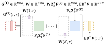
Figure 5: Computation for $\mathbf{G}^{(1)}=\mathbf{Y}_{(1)}(\mathbf{W}\odot\mathbf{V})$. The $r$th column $\mathbf{G}^{(1)}(:,r)$ of $\mathbf{G}^{(1)}$ is computed by $\left(\sum_{k=1}^{K}{\mathbf{W}(k,r)\left(\mathbf{P}_{k}\mathbf{Z}_{k}^{T}\mathbf{F}^{(k)}\right)}\right)\mathbf{E}\mathbf{D}^{T}\mathbf{V}(:,r)$.

Updating $\mathbf{H}$. In $\mathbf{Y}_{(1)}(\mathbf{W}\odot\mathbf{V})(\mathbf{W}^{T}\mathbf{W}*\mathbf{V}^{T}\mathbf{V})^{\dagger}$, we focus on efficiently computing $\mathbf{Y}_{(1)}(\mathbf{W}\odot\mathbf{V})$ based on Lemma 1. A naive computation for $\mathbf{Y}_{(1)}(\mathbf{W}\odot\mathbf{V})$ requires a high computational cost $\boldsymbol{\mathscr{O}}(JKR^{2})$ due to the explicit reconstruction of $\mathbf{Y}_{(1)}$. Therefore, we compute that term without the reconstruction by carefully determining the order of computations and exploiting the factorized matrices of $\mathbf{Y}_{(1)}$, $\mathbf{D}$, $\mathbf{E}$, $\mathbf{P}_{k}$, $\mathbf{Z}_{k}$, and $\mathbf{F}^{(k)}$ for $k=1,...,K$. With Lemma 1, we reduce the computational cost of $\mathbf{Y}_{(1)}(\mathbf{W}\odot\mathbf{V})$ to $\boldsymbol{\mathscr{O}}(JR^{2}+KR^{3})$.

Lemma 1.

Let us denote $\mathbf{Y}_{(1)}(\mathbf{W}\odot\mathbf{V})$ with $\mathbf{G}^{(1)}\in\mathbb{R}^{R\times R}$. $\mathbf{G}^{(1)}(:,r)$ is equal to $\left(\left(\sum_{k=1}^{K}{\mathbf{W}(k,r)\left(\mathbf{P}_{k}\mathbf{Z}_{k}^{T}\mathbf{F}^{(k)}\right)}\right)\mathbf{E}\mathbf{D}^{T}\mathbf{V}(:,r)\right)$. $\Box$

Proof.

$\mathbf{Y}_{(1)}$ is represented as follows:

$$\mathbf{Y}_{(1)} =\begin{bmatrix}\mathbf{P}_{1}\mathbf{Z}_{1}^{T}\mathbf{F}^{(1)}\mathbf{E}\mathbf{D}^{T}&;\cdots;&\mathbf{P}_{K}\mathbf{Z}_{K}^{T}\mathbf{F}^{(K)}\mathbf{E}\mathbf{D}^{T}\end{bmatrix}$$

$$=\left(\mathbin{\|}_{k=1}^{K}{\left(\mathbf{P}_{k}\mathbf{Z}_{k}^{T}\mathbf{F}^{(k)}\right)}\right)\begin{bmatrix}\mathbf{E}\mathbf{D}^{T}&\cdots&\mathbf{O}\\ \vdots&\ddots&\vdots\\ \mathbf{O}&\cdots&\mathbf{E}\mathbf{D}^{T}\end{bmatrix}$$

$$=\left(\mathbin{\|}_{k=1}^{K}{\left(\mathbf{P}_{k}\mathbf{Z}_{k}^{T}\mathbf{F}^{(k)}\right)}\right)\left(\mathbf{I}_{K\times K}\otimes\mathbf{E}\mathbf{D}^{T}\right)$$

where $\mathbf{I}_{K\times K}$ is the identity matrix of size $K\times K$. Then, $\mathbf{G}^{(1)}=\mathbf{Y}_{(1)}(\mathbf{W}\odot\mathbf{V})$ is expressed as follows:

$$\mathbf{G}^{(1)} =\left(\mathbin{\|}_{k=1}^{K}{\left(\mathbf{P}_{k}\mathbf{Z}_{k}^{T}\mathbf{F}^{(k)}\right)}\right)$$

$$\times\left(\mathbf{I}_{K\times K}\otimes\mathbf{E}\mathbf{D}^{T}\right)\left(\mathbin{\|}_{r=1}^{R}{\left(\mathbf{W}(:,r)\otimes\mathbf{V}(:,r)\right)}\right)$$

$$=\left(\mathbin{\|}_{k=1}^{K}{\left(\mathbf{P}_{k}\mathbf{Z}_{k}^{T}\mathbf{F}^{(k)}\right)}\right)\left(\mathbin{\|}_{r=1}^{R}{\left(\mathbf{W}(:,r)\otimes\mathbf{E}\mathbf{D}^{T}\mathbf{V}(:,r)\right)}\right)$$

The mixed-product property (i.e., $(\mathbf{A}\otimes\mathbf{B})(\mathbf{C}\otimes\mathbf{D})=\mathbf{A}\mathbf{C}\otimes\mathbf{B}\mathbf{D})$) is used in the above equation. Therefore, $\mathbf{G}^{(1)}(:,r)$ is equal to $\left(\mathbin{\|}_{k=1}^{K}{\left(\mathbf{P}_{k}\mathbf{Z}_{k}^{T}\mathbf{F}^{(k)}\right)}\right)\left(\mathbf{W}(:,r)\otimes\mathbf{E}\mathbf{D}^{T}\mathbf{V}(:,r)\right)$. We represent it as $\sum_{k=1}^{K}{\mathbf{W}(k,r)\left(\mathbf{P}_{k}\mathbf{Z}_{k}^{T}\mathbf{F}^{(k)}\right)}$ $\mathbf{E}\mathbf{D}^{T}\mathbf{V}(:,r)$ using block matrix multiplication since the $k$-th vertical block vector of $\left(\mathbf{W}(:,r)\otimes\mathbf{E}\mathbf{D}^{T}\mathbf{V}(:,r)\right)\in\mathbb{R}^{KR}$ is $\mathbf{W}(k,r)\mathbf{E}\mathbf{D}^{T}\mathbf{V}(:,r)\in\mathbb{R}^{R}$. ∎

As shown in Fig. 5, we compute $\mathbf{Y}_{(1)}(\mathbf{W}\odot\mathbf{V})$ column by column. In computing $\mathbf{G}^{(1)}(:,r)$, we compute $\mathbf{E}\mathbf{D}^{T}\mathbf{V}(:,r)$, sum up $\mathbf{W}(k,r)\left(\mathbf{P}_{k}\mathbf{Z}_{k}^{T}\mathbf{F}^{(k)}\right)$ for all $k$, and then perform matrix multiplication between the two preceding results (line 14 in Algorithm 3). After computing $\mathbf{G}^{(1)}\leftarrow\mathbf{Y}_{(1)}(\mathbf{W}\odot\mathbf{V})$, we update $\mathbf{H}$ by computing $\mathbf{G}^{(1)}(\mathbf{W}^{T}\mathbf{W}*\mathbf{V}^{T}\mathbf{V})^{\dagger}$ where ${\dagger}$ denotes the Moore-Penrose pseudoinverse (line 15 in Algorithm 3). Note that the pseudoinverse operation requires a lower computational cost compared to computing $\mathbf{G}^{(1)}$ since the size of $(\mathbf{W}^{T}\mathbf{W}*\mathbf{V}^{T}\mathbf{V})\in\mathbb{R}^{R\times R}$ is small.

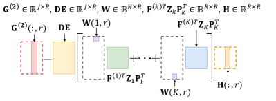
Figure 6: Computation for $\mathbf{G}^{(2)}=\mathbf{Y}_{(2)}(\mathbf{W}\odot\mathbf{H})$. The $r$th column $\mathbf{G}^{(2)}(:,r)$ of $\mathbf{G}^{(2)}$ is computed by $\mathbf{D}\mathbf{E}\sum_{k=1}^{K}{\left(\mathbf{W}(k,r)\mathbf{F}^{(k)T}\mathbf{Z}_{k}\mathbf{P}_{k}^{T}\mathbf{H}(:,r)\right)}$.

Updating $\mathbf{V}$. In computing $\mathbf{Y}_{(2)}(\mathbf{W}\odot\mathbf{U})(\mathbf{W}^{T}\mathbf{W}*\mathbf{U}^{T}\mathbf{U})^{\dagger}$, we need to efficiently compute $\mathbf{Y}_{(2)}(\mathbf{W}\odot\mathbf{U})$ based on Lemma 2. As in updating $\mathbf{H}$, a naive computation for $\mathbf{Y}_{(2)}(\mathbf{W}\odot\mathbf{U})$ requires a high computational cost $\boldsymbol{\mathscr{O}}(JKR^{2})$. We efficiently compute $\mathbf{Y}_{(2)}(\mathbf{W}\odot\mathbf{U})$ with the cost $\boldsymbol{\mathscr{O}}(JR^{2}+KR^{3})$, by carefully determining the order of computations and exploiting the factorized matrices of $\mathbf{Y}_{(2)}$.

Lemma 2.

Let us denote $\mathbf{Y}_{(2)}(\mathbf{W}\odot\mathbf{H})$ with $\mathbf{G}^{(2)}\in\mathbb{R}^{J\times R}$. $\mathbf{G}^{(2)}(:,r)$ is equal to $\mathbf{D}\mathbf{E}\left(\sum_{k=1}^{K}{\left(\mathbf{W}(k,r)\mathbf{F}^{(k)T}\mathbf{Z}_{k}\mathbf{P}_{k}^{T}\mathbf{H}(:,r)\right)}\right)$. $\Box$

Proof.

$\mathbf{Y}_{(2)}$ is represented as follows:

$$\mathbf{Y}_{(2)} =\begin{bmatrix}\mathbf{D}\mathbf{E}\mathbf{F}^{(1)T}\mathbf{Z}_{1}\mathbf{P}_{1}^{T}&;\cdots;&\mathbf{D}\mathbf{E}\mathbf{F}^{(K)T}\mathbf{Z}_{K}\mathbf{P}_{K}^{T}\end{bmatrix}$$

$$=\mathbf{D}\mathbf{E}\left(\mathbin{\|}_{k=1}^{K}{\mathbf{F}^{(k)T}\mathbf{Z}_{k}\mathbf{P}_{k}^{T}}\right)$$

Then, $\mathbf{G}^{(2)}=\mathbf{Y}_{(2)}(\mathbf{W}\odot\mathbf{H})$ is expressed as follows:

$$\mathbf{G}^{(2)} =\mathbf{D}\mathbf{E}\left(\mathbin{\|}_{k=1}^{K}{\mathbf{F}^{(k)T}\mathbf{Z}_{k}\mathbf{P}_{k}^{T}}\right)$$

$$\times\begin{bmatrix}\mathbf{W}(1,1)\mathbf{H}(:,1);&\cdots&;\mathbf{W}(1,R)\mathbf{H}(:,R)\\ \vdots&\vdots&\vdots\\ \mathbf{W}(K,1)\mathbf{H}(:,1);&\cdots&;\mathbf{W}(K,R)\mathbf{H}(:,R)\end{bmatrix}$$

$\mathbf{G}^{(2)}(:,r)$ is equal to $\mathbf{D}\mathbf{E}\sum_{k=1}^{K}{\left(\mathbf{W}(k,r)\mathbf{F}^{(k)T}\mathbf{Z}_{k}\mathbf{P}_{k}^{T}\mathbf{H}(:,r)\right)}$ according to the above equation. ∎

As shown in Fig. 6, we compute $\mathbf{G}^{(2)}\leftarrow\mathbf{Y}_{(2)}(\mathbf{W}\odot\mathbf{H})$ column by column. After computing $\mathbf{G}^{(2)}$, we update $\mathbf{V}$ by computing $\mathbf{G}^{(2)}(\mathbf{W}^{T}\mathbf{W}*\mathbf{H}^{T}\mathbf{H})^{\dagger}$ (lines 16 and 17 in Algorithm 3).

Updating $\mathbf{W}$. In computing $\mathbf{Y}_{(3)}(\mathbf{V}\odot\mathbf{H})(\mathbf{V}^{T}\mathbf{V}*\mathbf{H}^{T}\mathbf{H})^{\dagger}$, we efficiently compute $\mathbf{Y}_{(3)}(\mathbf{V}\odot\mathbf{H})$ based on Lemma 3. As in updating $\mathbf{H}$ and $\mathbf{V}$, a naive computation for $\mathbf{Y}_{(3)}(\mathbf{V}\odot\mathbf{H})$ requires a high computational cost $\boldsymbol{\mathscr{O}}(JKR^{2})$. We compute $\mathbf{Y}_{(3)}(\mathbf{V}\odot\mathbf{H})$ with the cost $\boldsymbol{\mathscr{O}}(JR^{2}+KR^{3})$ based on Lemma 3. Exploiting the factorized matrices of $\mathbf{Y}_{(3)}$ and carefully determining the order of computations improves the efficiency.

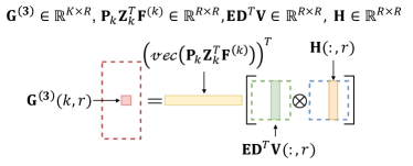
Figure 7: Computation for $\mathbf{G}^{(3)}=\mathbf{Y}_{(3)}(\mathbf{V}\odot\mathbf{H})$. $\mathbf{G}^{(3)}(k,r)$ is computed by $\left(vec\left(\mathbf{P}_{k}\mathbf{Z}_{k}^{T}\mathbf{F}^{(k)}\right)\right)^{T}\left(\mathbf{E}\mathbf{D}^{T}\mathbf{V}(:,r)\otimes\mathbf{H}(:,r)\right)$.

Lemma 3.

Let us denote $\mathbf{Y}_{(3)}(\mathbf{V}\odot\mathbf{H})$ with $\mathbf{G}^{(3)}\in\mathbb{R}^{K\times R}$. $\mathbf{G}^{(3)}(k,r)$ is equal to $\left(vec\left(\mathbf{P}_{k}\mathbf{Z}_{k}^{T}\mathbf{F}^{(k)}\right)\right)^{T}\left(\mathbf{E}\mathbf{D}^{T}\mathbf{V}(:,r)\otimes\mathbf{H}(:,r)\right)$ where $vec(\cdot)$ denotes the vectorization of a matrix. $\Box$

Proof.

$\mathbf{Y}_{(3)}$ is represented as follows:

$$\mathbf{Y}_{(3)} =\begin{bmatrix}\left(vec\left(\mathbf{P}_{1}\mathbf{Z}_{1}^{T}\mathbf{F}^{(1)}\mathbf{E}\mathbf{D}^{T}\right)\right)^{T}\\ \vdots\\ \left(vec\left(\mathbf{P}_{K}\mathbf{Z}_{K}^{T}\mathbf{F}^{(K)}\mathbf{E}\mathbf{D}^{T}\right)\right)^{T}\end{bmatrix}$$

$$=\left(\mathbin{\|}_{k=1}^{K}{\left(vec\left(\mathbf{P}_{k}\mathbf{Z}_{k}^{T}\mathbf{F}^{(k)}\mathbf{E}\mathbf{D}^{T}\right)\right)}\right)^{T}$$

$$=\left(\mathbin{\|}_{k=1}^{K}{\left(\mathbf{D}\mathbf{E}\otimes\mathbf{I}\right)vec\left(\mathbf{P}_{k}\mathbf{Z}_{k}^{T}\mathbf{F}^{(k)}\right)}\right)^{T}$$

$$=\left(\mathbin{\|}_{k=1}^{K}{\left(vec\left(\mathbf{P}_{k}\mathbf{Z}_{k}^{T}\mathbf{F}^{(k)}\right)\right)}\right)^{T}\left(\mathbf{E}\mathbf{D}^{T}\otimes\mathbf{I}_{R\times R}\right)$$

where $\mathbf{I}_{R\times R}$ is the identity matrix of size $R\times R$. The property of the vectorization (i.e., $vec(\mathbf{A}\mathbf{B})=(\mathbf{B}^{T}\otimes\mathbf{I})vec(\mathbf{A})$) is used. Then, $\mathbf{G}^{(3)}=\mathbf{Y}_{(3)}(\mathbf{V}\odot\mathbf{H})$ is expressed as follows:

$$\mathbf{G}^{(3)} =\left(\mathbin{\|}_{k=1}^{K}{\left(vec\left(\mathbf{P}_{k}\mathbf{Z}_{k}^{T}\mathbf{F}^{(k)}\right)\right)}\right)^{T}$$

$$\times\left(\mathbin{\|}_{r=1}^{R}{\left(\mathbf{E}\mathbf{D}^{T}\mathbf{V}(:,r)\otimes\mathbf{H}(:,r)\right)}\right)$$

$\mathbf{G}^{(3)}(k,r)$ is $\left(vec\left(\mathbf{P}_{k}\mathbf{Z}_{k}^{T}\mathbf{F}^{(k)}\right)\right)^{T}\left(\mathbf{E}\mathbf{D}^{T}\mathbf{V}(:,r)\otimes\mathbf{H}(:,r)\right)$ according to the above equation. ∎

We compute $\mathbf{G}^{(3)}=\mathbf{Y}_{(3)}(\mathbf{V}\odot\mathbf{H})$ row by row. Fig. 7 shows how we compute $\mathbf{G}^{(3)}(k,r)$. In computing $\mathbf{G}^{(3)}$, we first compute $\mathbf{E}\mathbf{D}^{T}\mathbf{V}$, and then obtain $\mathbf{G}^{(3)}(k,:)$ for all $k$ (line 18 in Algorithm 3). After computing $\mathbf{G}^{(3)}$, we update $\mathbf{W}$ by computing $\mathbf{G}^{(3)}(\mathbf{V}^{T}\mathbf{V}*\mathbf{H}^{T}\mathbf{H})^{\dagger}$ where ${\dagger}$ denotes the Moore-Penrose pseudoinverse (line 19 in Algorithm 3). We obtain $\mathbf{S}_{k}$ whose diagonal elements correspond to the $k$th row vector of $\mathbf{W}$ (line 21 in Algorithm 3).

After convergence, we obtain the factor matrices, ($\mathbf{U}_{k}\leftarrow\mathbf{A}_{k}\mathbf{Z}_{k}\mathbf{P}_{k}^{T}\mathbf{H}$ $=\mathbf{Q}_{k}\mathbf{H}$), $\mathbf{S}_{k}$, and $\mathbf{V}$ (line 25 in Algorithm 3).

Convergence Criterion. At the end of each iteration, we determine whether to stop or not (line 23 in Algorithm 3) based on the variation of $e=\left(\sum_{k=1}^{K}\|\mathbf{X}_{k}-\hat{\mathbf{X}}_{k}\|_{\mathbf{F}}^{2}\right)$ where $\hat{\mathbf{X}}_{k}=\mathbf{Q}_{k}\mathbf{H}\mathbf{S}_{k}\mathbf{V}^{T}$ is the $k$th reconstructed slice. However, measuring reconstruction errors $\sum_{k=1}^{K}\|\mathbf{X}_{k}-\hat{\mathbf{X}}_{k}\|_{\mathbf{F}}^{2}$ is inefficient since it requires high time and space costs proportional to input slices $\mathbf{X}_{k}$. To efficiently verify the convergence, our idea is to exploit $\mathbf{A}_{k}\mathbf{F}^{(k)}\mathbf{E}\mathbf{D}^{T}$ instead of $\mathbf{X}_{k}$, since the objective of our update process is to minimize the difference between $\mathbf{A}_{k}\mathbf{F}^{(k)}\mathbf{E}\mathbf{D}^{T}$ and $\hat{\mathbf{X}}_{k}=\mathbf{Q}_{k}\mathbf{H}\mathbf{S}_{k}\mathbf{V}^{T}$. With this idea, we improve the efficiency by computing $\sum_{k=1}^{K}\|\mathbf{P}_{k}\mathbf{Z}_{k}^{T}\mathbf{F}^{(k)}\mathbf{E}\mathbf{D}^{T}-\mathbf{H}\mathbf{S}_{k}\mathbf{V}^{T}\|_{\mathbf{F}}^{2}$, not the reconstruction errors. Our computation requires the time $\boldsymbol{\mathscr{O}}(JKR^{2})$ and space costs $\boldsymbol{\mathscr{O}}(JKR)$ which are much lower than the costs $\boldsymbol{\mathscr{O}}(\sum_{k=1}^{K}{I_{k}JR})$ and $\boldsymbol{\mathscr{O}}(\sum_{k=1}^{K}{I_{k}J})$ of naively computing $\sum_{k=1}^{K}\|\mathbf{X}_{k}-\hat{\mathbf{X}}_{k}\|_{\mathbf{F}}^{2}$, respectively. From $\|\mathbf{P}_{k}\mathbf{Z}_{k}^{T}\mathbf{F}^{(k)}\mathbf{E}\mathbf{D}^{T}-\mathbf{H}\mathbf{S}_{k}\mathbf{V}^{T}\|_{\mathbf{F}}^{2}$, we derive $\|\mathbf{A}_{k}\mathbf{F}^{(k)}\mathbf{E}\mathbf{D}^{T}-\hat{\mathbf{X}}_{k}\|_{\mathbf{F}}^{2}$. Since the Frobenius norm is unitarily invariant, we modify the computation as follows:

$$\|\mathbf{P}_{k}\mathbf{Z}_{k}^{T}\mathbf{F}^{(k)}\mathbf{E}\mathbf{D}^{T}-\mathbf{H}\mathbf{S}_{k}\mathbf{V}^{T}\|_{\mathbf{F}}^{2}$$

$$=\|\mathbf{Q}_{k}\mathbf{P}_{k}\mathbf{Z}_{k}^{T}\mathbf{F}^{(k)}\mathbf{E}\mathbf{D}^{T}-\mathbf{Q}_{k}\mathbf{H}\mathbf{S}_{k}\mathbf{V}^{T}\|_{\mathbf{F}}^{2}$$

$$=\|\mathbf{A}_{k}\mathbf{Z}_{k}\mathbf{P}_{k}^{T}\mathbf{P}_{k}\mathbf{Z}_{k}^{T}\mathbf{F}^{(k)}\mathbf{E}\mathbf{D}^{T}-\mathbf{Q}_{k}\mathbf{H}\mathbf{S}_{k}\mathbf{V}^{T}\|_{\mathbf{F}}^{2}$$

$$=\|\mathbf{A}_{k}\mathbf{F}^{(k)}\mathbf{E}\mathbf{D}^{T}-\hat{\mathbf{X}}_{k}\|_{\mathbf{F}}^{2}$$

where $\mathbf{P}_{k}^{T}\mathbf{P}_{k}$ and $\mathbf{Z}_{k}\mathbf{Z}_{k}^{T}$ are equal to $\mathbf{I}\in\mathbb{R}^{R\times R}$ since $\mathbf{P}_{k}$ and $\mathbf{Z}_{k}$ are orthonormal matrices. Note that the size of $\mathbf{P}_{k}\mathbf{Z}_{k}^{T}\mathbf{F}^{(k)}\mathbf{E}\mathbf{D}^{T}$ and $\mathbf{H}\mathbf{S}_{k}\mathbf{V}^{T}$ is $R\times J$ which is much smaller than the size $I_{k}\times J$ of input slices $\mathbf{X}_{k}$. This modification completes the efficiency of our update rule.

1

0:  the number $T$ of threads, $\mathbf{X}_{k}\in\mathbb{R}^{I_{k}\times J}$ for $k=1,...,K$

0:  sets $\boldsymbol{\mathscr{T}}_{i}$ for $i=1,...,T$.

1:  initialize $\boldsymbol{\mathscr{T}}_{i}\leftarrow\emptyset$ for $i=1,...,T$.

2:  construct a list $S$ of size $T$ whose elements are zero

23:  construct a list $L_{init}$ containing the number of rows of $\mathbf{X}_{k}$ for $k=1,...,K$

34:  sort $L_{init}$ in descending order, and obtain lists $L_{val}$ and $L_{ind}$ that contain sorted values and those corresponding indices

5:  for $k=1,...,K$ do

46:     $t_{min}\leftarrow\operatorname*{argmin}S$

57:     $l\leftarrow L_{ind}[k]$

68:     $\boldsymbol{\mathscr{T}}_{t_{min}}\leftarrow\boldsymbol{\mathscr{T}}_{t_{min}}\cup\{\mathbf{X}_{l}\}$

9:     $S[t_{min}]\leftarrow S[t_{min}]+L_{val}[k]$

10:  end for

Algorithm 4 Careful distribution of work in DPar2

III-F Careful distribution of work

The last challenge for an efficient and scalable PARAFAC2 decomposition method is how to parallelize the computations described in Sections III-B to III-E. Although a previous work [11] introduces the parallelization with respect to the $K$ slices, there is still a room for maximizing parallelism. Our main idea is to carefully allocate input slices $\mathbf{X}_{k}$ to threads by considering the irregularity of a given tensor.

The most expensive operation is to compute randomized SVD of input slices $\mathbf{X}_{k}$ for all $k$; thus we first focus on how well we parallelize this computation (i.e., lines 2 to 4 in Algorithm 3). A naive approach is to randomly allocate input slices to threads, and let each thread compute randomized SVD of the allocated slices. However, the completion time of each thread can vary since the computational cost of computing randomized SVD is proportional to the number of rows of slices; the number of rows of input slices is different from each other as shown in Fig. 8. Therefore, we need to distribute $\mathbf{X}_{k}$ fairly across each thread considering their numbers of rows.

For $i=1,..,T$, consider that an $i$th thread performs randomized SVD for slices in a set $\boldsymbol{\mathscr{T}}_{i}$ where $T$ is the number of threads. To reduce the completion time, the sums of rows of slices in the sets should be nearly equal to each other. To achieve it, we exploit a greedy number partitioning technique that repeatedly adds a slice into a set with the smallest sum of rows. Algorithm 4 describes how to construct the sets $\boldsymbol{\mathscr{T}}_{i}$ for compressing input slices in parallel. Let $L_{init}$ be a list containing the number of rows of $\mathbf{X}_{k}$ for $k=1,...,K$ (line 3 in Algorithm 4). We first obtain lists $L_{val}$ and $L_{ind}$, sorted values and those corresponding indices, by sorting $L_{init}$ in descending order (line 4 in Algorithm 4). We repeatedly add a slice $\mathbf{X}_{k}$ to a set $\boldsymbol{\mathscr{T}}_{i}$ that has the smallest sum. For each $k$, we find the index $t_{min}$ of the minimum in $S$ whose $i$th element corresponds to the sum of row sizes of slices in the $i$th set $\boldsymbol{\mathscr{T}}_{i}$ (line 6 in Algorithm 4). Then, we add a slice $\mathbf{X}_{l}$ to the set $\boldsymbol{\mathscr{T}}_{t_{min}}$ where $l$ is equal to $L_{ind}[k]$, and update the list $S$ by $S[t_{min}]\leftarrow S[t_{min}]+L_{val}[k]$ (lines 7 to 9 in Algorithm 4). Note that $S[k]$, $L_{ind}[k]$, and $L_{val}[k]$ denote the $k$th element of $S$, $L_{ind}$, and $L_{val}$, respectively. After obtaining the sets $\boldsymbol{\mathscr{T}}_{i}$ for $i=1,..,T$, $i$th thread performs randomized SVD for slices in the set $\boldsymbol{\mathscr{T}}_{i}$.

After decomposing $\mathbf{X}_{k}$ for all $k$, we do not need to consider the irregularity for parallelism since there is no computation with $\mathbf{A}_{k}$ which involves the irregularity. Therefore, we uniformly allocate computations across threads for all $k$ slices. In each iteration (lines 8 to 22 in Algorithm 3), we easily parallelize computations. First, we parallelize the iteration (lines 8 to 10) for all $k$ slices. To update $\mathbf{H}$, $\mathbf{V}$, and $\mathbf{W}$, we need to compute $\mathbf{G}^{(1)}$, $\mathbf{G}^{(2)}$, and $\mathbf{G}^{(3)}$ in parallel. In Lemmas 1 and 2, DPar2 parallelly computes $\mathbf{W}(k,r)\left(\mathbf{P}_{k}\mathbf{Z}_{k}^{T}\mathbf{F}^{(k)}\right)$ and $\mathbf{W}(k,r)\mathbf{F}^{(k)}\mathbf{Z}_{k}\mathbf{P}_{k}^{T}\mathbf{H}(:,r)$ for $k$, respectively. In Lemma 3, DPar2 parallelly computes $\left(vec\left(\mathbf{P}_{k}\mathbf{Z}_{k}^{T}\mathbf{F}^{(k)}\right)\right)^{T}\left(\mathbf{E}\mathbf{D}^{T}\mathbf{V}(:,r)\otimes\mathbf{H}(:,r)\right)$ for $k$.

(a) US stock data

(b) KR stock data

Figure 8: The length of temporal dimension of input slices $\mathbf{X}_{k}$ on US Stock and Korea Stock data. We sort the lengths in descending order.

III-G Complexities

We analyze the time complexity of DPar2.

Lemma 4.

Compressing input slices takes $\boldsymbol{\mathscr{O}}\left(\left(\sum_{k=1}^{K}{I_{k}JR}\right)+JKR^{2}\right)$ time.

Proof.

The SVD in the first stage takes $\boldsymbol{\mathscr{O}}\left(\sum_{k=1}^{K}{I_{k}JR}\right)$ times since computing randomized SVD of $\mathbf{X}_{k}$ takes $\boldsymbol{\mathscr{O}}(I_{k}JR)$ time. Then, the SVD in the second stage takes $\boldsymbol{\mathscr{O}}\left(JKR^{2}\right)$ due to randomized SVD of $\mathbf{M}_{(2)}\in\mathbb{R}^{J\times KR}$. Therefore, the time complexity of the SVD in the two stages is $\boldsymbol{\mathscr{O}}\left(\left(\sum_{k=1}^{K}{I_{k}JR}\right)+JKR^{2}\right)$. ∎

Lemma 5.

At each iteration, computing $\mathbf{Y}_{k}$ and updating $\mathbf{H}$, $\mathbf{V}$, and $\mathbf{W}$ takes $\boldsymbol{\mathscr{O}}(JR^{2}+KR^{3})$ time.

Proof.

For $\mathbf{Y}_{k}$, computing $\mathbf{F}^{(k)}\mathbf{E}\mathbf{D}^{T}\mathbf{V}\mathbf{S}_{k}\mathbf{H}^{T}$ and performing SVD of it for all $k$ take $\boldsymbol{\mathscr{O}}(JR^{2}+KR^{3})$. Updating each of $\mathbf{H}$, $\mathbf{V}$, and $\mathbf{W}$ takes $\boldsymbol{\mathscr{O}}(JR^{2}+KR^{3}+R^{3})$ time. Therefore, the complexity for $\mathbf{Y}_{k}$, $\mathbf{H}$, $\mathbf{V}$, and $\mathbf{W}$ is $\boldsymbol{\mathscr{O}}\left(JR^{2}+KR^{3}\right)$. ∎

Theorem 1.

The time complexity of DPar2 is $\boldsymbol{\mathscr{O}}\left(\left(\sum_{k=1}^{K}{I_{k}JR}\right)+JKR^{2}+MKR^{3}\right)$ where $M$ is the number of iterations.

Proof.

The overall time complexity of DPar2 is the summation of the compression cost (see Lemma 4) and the iteration cost (see Lemma 5): $\boldsymbol{\mathscr{O}}\left(\left(\sum_{k=1}^{K}{I_{k}JR}\right)+JKR^{2}+M(JR^{2}+KR^{3})\right)$. Note that $MJR^{2}$ term is omitted since it is much smaller than $\left(\sum_{k=1}^{K}{I_{k}JR}\right)$ and $JKR^{2}$. ∎

Theorem 2.

The size of preprocessed data of DPar2 is $\boldsymbol{\mathscr{O}}\left(\left(\sum_{k=1}^{K}{I_{k}R}\right)+KR^{2}+JR\right)$.

Proof.

The size of preprocessed data of DPar2 is proportional to the size of $\mathbf{E}$, $\mathbf{D}$, $\mathbf{A}_{k}$, and $\mathbf{F}^{(k)}$ for $k=1,...,K$. The size of $\mathbf{E}$ and $\mathbf{D}$ is $R$ and $J\times R$, respectively. For each $k$, the size of $\mathbf{A}$ and $\mathbf{F}$ is $I_{k}\times R$ and $R\times R$, respectively. Therefore, the size of preprocessed data of DPar2 is $\boldsymbol{\mathscr{O}}\left(\left(\sum_{k=1}^{K}{I_{k}R}\right)+KR^{2}+JR\right)$. ∎

IV Experiments

TABLE II: Description of real-world tensor datasets.

Dataset	Max Dim. $I_{k}$	Dim. $J$	Dim. $K$	Summary
FMA1 [26]	$704$	$2,049$	$7,997$	music
Urban2 [27]	$174$	$2,049$	$8,455$	urban sound
US Stock3	$7,883$	$88$	$4,742$	stock
Korea Stock4 [3]	$5,270$	$88$	$3,664$	stock
Activity5 [28, 29]	$553$	$570$	$320$	video feature
Action5 [28, 29]	$936$	$570$	$567$	video feature
Traffic6 [30]	$2,033$	$96$	$1,084$	traffic
PEMS-SF7	$963$	$144$	$440$	traffic

(a) Preprocessing time

(b) Iteration time

Figure 9: [Best viewed in color] (a) DPar2 efficiently preprocesses a given irregular dense tensor, which is up to $10\times$ faster compared to RD-ALS. (b) At each iteration, DPar2 runs by up to $10.3\times$ faster than the second best method.

In this section, we experimentally evaluate the performance of DPar2. We answer the following questions:

Performance (Section IV-B). How quickly and accurately does DPar2 perform PARAFAC2 decomposition compared to other methods?

Data Scalability (Section IV-C). How well does DPar2 scale up with respect to tensor size and target rank?

Multi-core Scalability (Section IV-D). How much does the number of threads affect the running time of DPar2?

Discovery (Section IV-E). What can we discover from real-world tensors using DPar2?

IV-A Experimental Settings

We describe experimental settings for the datasets, competitors, parameters, and environments.

Machine. We use a workstation with $2$ CPUs (Intel Xeon E5-2630 v4 @ 2.2GHz), each of which has $10$ cores, and 512GB memory for the experiments.

Real-world Data. We evaluate the performance of DPar2 and competitors on real-world datasets summarized in Table II. FMA dataset [26] is the collection of songs. Urban Sound dataset [27] is the collection of urban sounds such as drilling, siren, and street music. For the two datasets, we convert each time series into an image of a log-power spectrogram so that their forms are (time, frequency, song; value) and (time, frequency, sound; value), respectively. US Stock dataset is the collection of stocks on the US stock market. Korea Stock dataset [3] is the collection of stocks on the South Korea stock market. Each stock is represented as a matrix of (date, feature) where the feature dimension includes 5 basic features and 83 technical indicators. The basic features collected daily are the opening, the closing, the highest, and the lowest prices and trading volume, and technical indicators are calculated based on the basic features. The two stock datasets have the form of (time, feature, stock; value). Activity data and Action data⁵ are the collection of features for motion videos. The two datasets have the form of (frame, feature, video; value). We refer the reader to [28] for their feature extraction. Traffic data is the collection of traffic volume around Melbourne, and its form is (sensor, frequency, time; measurement). PEMS-SF data contain the occupancy rate of different car lanes of San Francisco bay area freeways: (station, timestamp, day; measurement). Traffic data and PEMS-SF data are 3-order regular tensors, but we can analyze them using PARAFAC2 decomposition approaches.

Figure 10: The size of preprocessed data. DPar2 generates up to $201\times$ smaller preprocessed data than input tensors used for SPARTan and PARAFAC2-ALS.

Synthetic Data. We evaluate the scalability of DPar2 and competitors on synthetic tensors. Given the number $K$ of slices, and the slice sizes $I$ and $J$, we generate a synthetic tensor using tenrand(I, J, K) function in Tensor Toolbox [31], which randomly generates a tensor $\boldsymbol{\mathscr{X}}\in\mathbb{R}^{I\times J\times K}$. We construct a tensor $\{\mathbf{X}_{k}\}_{k=1}^{K}$ where $\mathbf{X}_{k}$ is equal to $\boldsymbol{\mathscr{X}}(:,:,k)$ for $k=1,...K$.

Competitors. We compare DPar2 with PARAFAC2 decomposition methods based on ALS. All the methods including DPar2 are implemented in MATLAB (R2020b).

• DPar2: the proposed PARAFAC2 decomposition model which preprocesses a given irregular dense tensor and updates factor matrices using the preprocessing result.

• RD-ALS [18]: PARAFAC2 decomposition which preprocesses a given irregular tensor. Since there is no public code, we implement it using Tensor Toolbox [31] based on its paper [18].

• PARAFAC2-ALS: PARAFAC2 decomposition based on ALS approach. It is implemented based on Algorithm 2 using Tensor Toolbox [31].

• SPARTan [11]: fast and scalable PARAFAC2 decomposition for irregular sparse tensors. Although it targets on sparse irregular tensors, it can be adapted to irregular dense tensors. We use the code implemented by authors.

(a) Scalability for tensor size

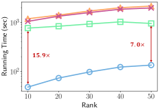
(b) Scalability for rank

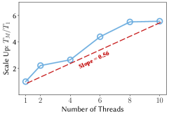
(c) Machine Scalability

Figure 11: Data scalability. DPar2 is more scalable than other PARAFAC2 decomposition methods in terms of both tensor size and rank. (a) DPar2 is $15.3\times$ faster than the second-fastest method on the irregular dense tensor of the total size $1.6\times 10^{10}$. (b) DPar2 is $7.0\times$ faster than the second-fastest method even when a high target rank is given. (c) Multi-core scalability with respect to the number of threads. $T_{M}$ indicates the running time of DPar2 on the number $M$ of threads. DPar2 gives near-linear scalability, and accelerates $5.5\times$ when the number of threads increases from $1$ to $10$.

Parameters. We use the following parameters.

• Number of threads: we use $6$ threads except in Section IV-D.

• Max number of iterations: the maximum number of iterations is set to $32$.

• Rank: we set the target rank $R$ to $10$ except in the trade-off experiments of Section IV-B and Section IV-D. We also set the rank of randomized SVD to $10$ which is the same as the target rank $R$ of PARAFAC2 decomposition.

To compare running time, we run each method $5$ times, and report the average.

Fitness. We evaluate the fitness defined as follows:

$$1-\left(\frac{\sum_{k=1}^{K}\|\mathbf{X}_{k}-\hat{\mathbf{X}}_{k}\|_{\mathbf{F}}^{2}}{\sum_{k=1}^{K}\|\mathbf{X}_{k}\|_{\mathbf{F}}^{2}}\right)$$

where $\mathbf{X}_{k}$ is the $k$-th input slice and $\hat{\mathbf{X}}_{k}$ is the $k$-th reconstructed slice of PARAFAC2 decomposition. Fitness close to $1$ indicates that a model approximates a given input tensor well.

IV-B Performance (Q1)

We evaluate the fitness and the running time of DPar2, RD-ALS, SPARTan, and PARAFAC2-ALS.

Trade-off. Fig. 1 shows that DPar2 provides the best trade-off of running time and fitness on real-world irregular tensors for the three target ranks: $10$, $15$, and $20$. DPar2 achieves $6.0\times$ faster running time than the competitors for FMA dataset while having a comparable fitness. In addition, DPar2 provides at least $1.5\times$ faster running times than the competitors for the other datasets. The performance gap is large for FMA and Urban datasets whose sizes are larger than those of the other datasets. It implies that DPar2 is more scalable than the competitors in terms of tensor sizes.

Preprocessing time. We compare DPar2 with RD-ALS and exclude SPARTan and PARAFAC2-ALS since only RD-ALS has a preprocessing step. As shown in Fig. 9(a), DPar2 is up to $10\times$ faster than RD-ALS. There is a large performance gap on FMA and Urban datasets since RD-ALS cannot avoid the overheads for the large tensors. RD-ALS performs SVD of the concatenated slice matrices $\mathbin{\|}_{k=1}^{K}{\mathbf{X}^{T}_{k}}$, which leads to its slow preprocessing time.

Iteration time. Fig. 9(b) shows that DPar2 outperforms competitors for running time at each iteration. Compared to SPARTan and PARAFAC2-ALS, DPar2 significantly reduces the running time per iteration due to the small size of the preprocessed results. Although RD-ALS reduces the computational cost at each iteration by preprocessing a given tensor, DPar2 is up to $10.3\times$ faster than RD-ALS. Compared to RD-ALS that computes the variation of $\left(\sum_{k=1}^{K}\|\mathbf{X}_{k}-\mathbf{Q}_{k}\mathbf{H}\mathbf{S}_{k}\mathbf{V}^{T}\|_{\mathbf{F}}^{2}\right)$ for the convergence criterion, DPar2 efficiently verifies the convergence by computing the variation of $\sum_{k=1}^{K}\|\mathbf{P}_{k}\mathbf{Z}_{k}^{T}\mathbf{F}^{(k)}\mathbf{E}\mathbf{D}^{T}-\mathbf{H}\mathbf{S}_{k}\mathbf{V}^{T}\|_{\mathbf{F}}^{2}$, which affects the running time at each iteration. In summary, DPar2 obtains $\mathbf{U}_{k}$, $\mathbf{S}_{k}$, and $\mathbf{V}$ in a reasonable running time even if the number of iterations increases.

Size of preprocessed data. We measure the size of preprocessed data on real-world datasets. For PARAFAC2-ALS and SPARTan, we report the size of input irregular tensor since they have no preprocessing step. Compared to an input irregular tensor, DPar2 generates much smaller preprocessed data by up to $201$ times as shown in Fig. 10. Given input slices $\mathbf{X}_{k}$ of size $I_{k}\times J$, the compression ratio increases as the number $J$ of columns increases; the compression ratio is larger on FMA, Urban, Activity, and Action datasets than on US Stock, KR Stock, Traffic, and PEMS-SF. This is because the compression ratio is proportional to $\frac{\text{Size of an irregular tensor}}{\text{Size of the preprocessed results}}\approx\frac{IJK}{IKR+KR^{2}+JR}=\frac{1}{R/J+R^{2}/IJ+R/IK}$ assuming $I_{1}=...=I_{K}=I$; $R/J$ is the dominant term which is much larger than $R^{2}/IJ$ and $R/IK$.

IV-C Data Scalability (Q2)

We evaluate the data scalability of DPar2 by measuring the running time on several synthetic datasets. We first compare the performance of DPar2 and the competitors by increasing the size of an irregular tensor. Then, we measure the running time by changing a target rank.

Tensor Size. To evaluate the scalability with respect to the tensor size, we generate $5$ synthetic tensors of the following sizes $I\times J\times K$: $\{1000\times 1000\times 1000,1000\times 1000\times 2000,2000\times 1000\times 2000,2000\times 2000\times 2000,2000\times 2000\times 4000\}$. For simplicity, we set $I_{1}=\cdots=I_{K}=I$. Fig. 11(a) shows that DPar2 is up to $15.3\times$ faster than competitors on all synthetic tensors; in addition, the slope of DPar2 is lower than that of competitors. Also note that only DPar2 obtains factor matrices of PARAFAC2 decomposition within a minute for all the datasets.

Rank. To evaluate the scalability with respect to rank, we generate the following synthetic data: $I_{1}=\cdots=I_{K}=2,000$, $J=2,000$, and $K=4,000$. Given the synthetic tensors, we measure the running time for $5$ target ranks: $10$, $20$, $30$, $40$, and $50$. DPar2 is up to $15.9\times$ faster than the second-fastest method with respect to rank in Fig. 11(b). For higher ranks, the performance gap slightly decreases since DPar2 depends on the performance of randomized SVD which is designed for a low target rank. Still, DPar2 is up to $7.0\times$ faster than competitors with respect to the highest rank used in our experiment.

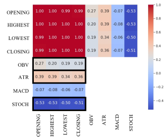
(a) US stock data

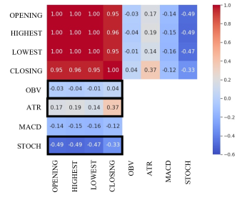
(b) Korea stock data

Figure 12: The similarity patterns of features are different on the two stock markets. (a) For US Stock data, ATR and OBV have a positive correlation with the price features. (b) For Korea Stock data, they are uncorrelated with the price features in general.

IV-D Multi-core Scalability (Q3)

We generate the following synthetic data: $I_{1}=\cdots=I_{K}=2,000$, $J=2,000$, and $K=4,000$, and evaluate the multi-core scalability of DPar2 with respect to the number of threads: $1,2,4,6,8,$ and $10$. $T_{M}$ indicates the running time when using the number $M$ of threads. As shown in Fig. 11(c), DPar2 gives near-linear scalability, and accelerates $5.5\times$ when the number of threads increases from $1$ to $10$.

IV-E Discoveries (Q4)

We discover various patterns using DPar2 on real-world datasets.

IV-E1 Feature Similarity on Stock Dataset

We measure the similarities between features on US Stock and Korea Stock datasets, and compare the results. We compute Pearson Correlation Coefficient (PCC) between $\mathbf{V}(i,:)$, which represents a latent vector of the $i$th feature. For effective visualization, we select 4 price features (the opening, the closing, the highest, and the lowest prices), and 4 representative technical indicators described as follows:

• OBV (On Balance Volume): a technical indicator for cumulative trading volume. If today’s closing price is higher than yesterday’s price, OBV increases by the amount of today’s volume. If not, OBV decreases by the amount of today’s volume.

• ATR (Average True Range): a technical indicator for volatility developed by J. Welles Wilder, Jr. It increases in high volatility while decreasing in low volatility.

• MACD (Moving Average Convergence and Divergence): a technical indicator for trend developed by Gerald Appel. It indicates the difference between long-term and short-term exponential moving averages (EMA).

• STOCH (Stochastic Oscillator): a technical indicator for momentum developed by George Lane. It indicates the position of the current closing price compared to the highest and the lowest prices in a duration.

Fig. 12(a) and 12(b) show correlation heatmaps for US Stock data and Korea Stock data, respectively. We analyze correlation patterns between price features and technical indicators. On both datasets, STOCH has a negative correlation and MACD has a weak correlation with the price features. On the other hand, OBV and ATR indicators have different patterns on the two datasets. On the US stock dataset, ATR and OBV have a positive correlation with the price features. On the Korea stock dataset, OBV has little correlation with the price features. Also, ATR has little correlation with the price features except for the closing price. These different patterns are due to the difference of the two markets in terms of market size, market stability, tax, investment behavior, etc.

IV-E2 Finding Similar Stocks

On US Stock dataset, which stock is similar to a target stock $s_{T}$ in a time range that a user is curious about? In this section, we provide analysis by setting the target stock $s_{T}$ to Microsoft (Ticker: MSFT), and the range a duration when the COVID-19 was very active (Jan. 2, 2020 - Apr. 15, 2021). We efficiently answer the question by 1) constructing the tensor included in the range, 2) obtaining factor matrices with DPar2, and 3) post-processing the factor matrices of DPar2. Since $\mathbf{U}_{k}$ represents temporal latent vectors of the $k$th stock, the similarity $sim(s_{i},s_{j})$ between stocks $s_{i}$ and $s_{j}$ is computed as follows:

$$sim(s_{i},s_{j})=\exp\left(-\gamma{{\|\mathbf{U}_{s_{i}}-\mathbf{U}_{s_{j}}\|_{F}^{2}}}\right)$$ (10)

where $\exp$ is the exponential function. We set $\gamma$ to $0.01$ in this section. Note that we use only the stocks that have the same target range since $\mathbf{U}_{s_{i}}-\mathbf{U}_{s_{j}}$ is defined only when the two matrices are of the same size.

Based on $sim(s_{i},s_{j})$, we find similar stocks to $s_{T}$ using two different techniques: 1) $k$-nearest neighbors, and 2) Random Walks with Restarts (RWR). The first approach simply finds stocks similar to the target stock, while the second one finds similar stocks by considering the multi-faceted relationship between stocks.

$k$-nearest neighbors. We compute $sim(s_{T},s_{j})$ for $j=1,...,K$ where $K$ is the number of stocks to be compared, and find top-$10$ similar stocks to $s_{T}$, Microsoft (Ticker: MSFT). In Table IV(a), the Microsoft stock is similar to stocks of the Technology sector or with a large capitalization (e.g., Amazon.com, Apple, and Alphabet) during the COVID-19. Moody’s is also similar to the target stock.

TABLE III: Based on the results of DPar2, we find similar stocks to Microsoft (MSFT) during the COVID-19. (a) Top-$10$ stocks from $k$-nearest neighbors. (b) Top-$10$ stocks from RWR. The blue color refers to the stocks that appear only in one of the two approaches among the top-10 stocks.

Rank	Stock Name	Sector
1	Adobe	Technology
2	Amazon.com	Consumer Cyclical
3	Apple	Technology
4	Moody’s	Financial Services
5	Intuit	Technology
6	ANSYS	Technology
7	Synopsys	Technology
8	Alphabet	Communication Services
9	ServiceNow	Technology
10	EPAM Systems	Technology

(a) Similarity based Result

Rank	Stock Name	Sector
1	Synopsys	Technology
2	ANSYS	Technology
3	Adobe	Technology
4	Amazon.com	Consumer Cyclical
5	Netflix	Communication Services
6	Autodesk	Technology
7	Apple	Technology
8	Moody’s	Financial Services
9	NVIDIA	Technology
10	S&P Global	Financial Services

(b) RWR Result

Random Walks with Restarts (RWR). We find similar stocks using another approach, Random Walks with Restarts (RWR) [32, 33, 34, 35]. To exploit RWR, we first a similarity graph based on the similarities between stocks. The elements of the adjacency matrix $\mathbf{A}$ of the graph is defined as follows:

$$\mathbf{A}(i,j)=\begin{cases}sim(s_{i},s_{j})&\text{if $i\neq j$}\\ 0&\text{if $i=j$}\end{cases}$$ (11)

We ignore self-loops by setting $\mathbf{A}(i,i)$ to $0$ for $i=1,...,K$.

After constructing the graph, we find similar stocks using RWR. The scores $\mathbf{r}$ is computed by using the power iteration [36] as described in [37]:

$$\mathbf{r}^{(i)}\leftarrow(1-c)\tilde{\mathbf{A}}^{T}\mathbf{r}^{(i-1)}+c\mathbf{q}$$ (12)

where $\tilde{\mathbf{A}}$ is the row-normalized adjacency matrix, $\mathbf{r}^{(i)}$ is the score vector at the $i$th iteration, $c$ is a restart probability, and $\mathbf{q}$ is a query vector. We set $c$ to $0.15$, the maximum iteration to $100$, and $\mathbf{q}$ to the one-hot vector where the element corresponding to Microsoft is 1, and the others are 0.

As shown in Table III, the common pattern of the two approaches is that many stocks among the top-10 belong to the technology sector. There is also a difference. In Table III, the blue color indicates the stocks that appear only in one of the two approaches among the top-10. In Table IV(a), the $k$-nearest neighbor approach simply finds the top-$10$ stocks which are closest to Microsoft based on distances. On the other hand, the RWR approach finds the top-$10$ stocks by considering more complicated relationships. There are $4$ stocks appearing only in Table IV(b). S&P Global is included since it is very close to Moody’s which is ranked $4$th in Table IV(a). Netflix, Autodesk, and NVIDIA are relatively far from the target stock compared to stocks such as Intuit and Alphabet, but they are included in the top-$10$ since they are very close to Amazon.com, Adobe, ANSYS, and Synopsys. This difference comes from the fact that the $k$-nearest neighbors approach considers only distances from the target stock while the RWR approach considers distances between other stocks in addition to the target stock.

DPar2 allows us to efficiently obtain factor matrices, and find interesting patterns in data.

V Related Works

We review related works on tensor decomposition methods for regular and irregular tensors.

Tensor decomposition on regular dense tensors. There are efficient tensor decomposition methods on regular dense tensors. Pioneering works [38, 39, 40, 41, 42, 43] efficiently decompose a regular tensor by exploiting techniques that reduce time and space costs. Also, a lot of works [44, 45, 46, 47] proposed scalable tensor decomposition methods with parallelization to handle large-scale tensors. However, the aforementioned methods fail to deal with the irregularity of dense tensors since they are designed for regular tensors.

PARAFAC2 decomposition on irregular tensors. Cheng and Haardt [18] proposed RD-ALS which preprocesses a given tensor and performs PARAFAC2 decomposition using the preprocessed result. However, RD-ALS requires high computational costs to preprocess a given tensor. Also, RD-ALS is less efficient in updating factor matrices since it computes reconstruction errors for the convergence criterion at each iteration. Recent works [11, 12, 15] attempted to analyze irregular sparse tensors. SPARTan [11] is a scalable PARAFAC2-ALS method for large electronic health records (EHR) data. COPA [12] improves the performance of PARAFAC2 decomposition by applying various constraints (e.g., smoothness). REPAIR [15] strengthens the robustness of PARAFAC2 decomposition by applying low-rank regularization. We do not compare DPar2 with COPA and REPAIR since they concentrate on imposing practical constraints to handle irregular sparse tensors, especially EHR data. However, we do compare DPar2 with SPARTan which the efficiency of COPA and REPAIR is based on. TASTE [16] is a joint PARAFAC2 decomposition method for large temporal and static tensors. Although the above methods are efficient in PARAFAC2 decomposition for irregular tensors, they concentrate only on irregular sparse tensors, especially EHR data. LogPar [17], a logistic PARAFAC2 decomposition method, analyzes temporal binary data represented as an irregular binary tensor. SPADE [48] efficiently deals with irregular tensors in a streaming setting. TedPar [49] improves the performance of PARAFAC2 decomposition by explicitly modeling the temporal dependency. Although the above methods effectively deal with irregular sparse tensors, especially EHR data, none of them focus on devising an efficient PARAFAC2 decomposition method on irregular dense tensors. On the other hand, DPar2 is a fast and scalable PARAFAC2 decomposition method for irregular dense tensors.

VI Conclusion

In this paper, we propose DPar2, a fast and scalable PARAFAC2 decomposition method for irregular dense tensors. By compressing an irregular input tensor, careful reordering of the operations with the compressed results in each iteration, and careful partitioning of input slices, DPar2 successfully achieves high efficiency to perform PARAFAC2 decomposition for irregular dense tensors. Experimental results show that DPar2 is up to $6.0\times$ faster than existing PARAFAC2 decomposition methods while achieving comparable accuracy, and it is scalable with respect to the tensor size and target rank. With DPar2, we discover interesting patterns in real-world irregular tensors. Future work includes devising an efficient PARAFAC2 decomposition method in a streaming setting.

References

- [1] Y.-R. Lin, J. Sun, P. Castro, R. Konuru, H. Sundaram, and A. Kelliher, “Metafac: community discovery via relational hypergraph factorization,” in KDD, 2009, pp. 527–536.
- [2] S. Spiegel, J. Clausen, S. Albayrak, and J. Kunegis, “Link prediction on evolving data using tensor factorization,” in PAKDD. Springer, 2011, pp. 100–110.
- [3] J.-G. Jang and U. Kang, “Fast and memory-efficient tucker decomposition for answering diverse time range queries,” in Proceedings of the 27th ACM SIGKDD Conference on Knowledge Discovery & Data Mining, 2021, pp. 725–735.
- [4] S. Oh, N. Park, J.-G. Jang, L. Sael, and U. Kang, “High-performance tucker factorization on heterogeneous platforms,” IEEE Transactions on Parallel and Distributed Systems, vol. 30, no. 10, pp. 2237–2248, 2019.
- [5] T. Kwon, I. Park, D. Lee, and K. Shin, “Slicenstitch: Continuous cp decomposition of sparse tensor streams,” in ICDE. IEEE, 2021, pp. 816–827.
- [6] D. Ahn, S. Kim, and U. Kang, “Accurate online tensor factorization for temporal tensor streams with missing values,” in CIKM ’21: The 30th ACM International Conference on Information and Knowledge Management, Virtual Event, Queensland, Australia, November 1 - 5, 2021, G. Demartini, G. Zuccon, J. S. Culpepper, Z. Huang, and H. Tong, Eds. ACM, 2021, pp. 2822–2826.
- [7] D. Ahn, J.-G. Jang, and U. Kang, “Time-aware tensor decomposition for sparse tensors,” Machine Learning, Sep 2021.
- [8] D. Ahn, S. Son, and U. Kang, “Gtensor: Fast and accurate tensor analysis system using gpus,” in CIKM ’20: The 29th ACM International Conference on Information and Knowledge Management, Virtual Event, Ireland, October 19-23, 2020, M. d’Aquin, S. Dietze, C. Hauff, E. Curry, and P. Cudré-Mauroux, Eds. ACM, 2020, pp. 3361–3364.
- [9] D. Choi, J.-G. Jang, and U. Kang, “S3cmtf: Fast, accurate, and scalable method for incomplete coupled matrix-tensor factorization,” PLOS ONE, vol. 14, no. 6, pp. 1–20, 06 2019.
- [10] N. Park, S. Oh, and U. Kang, “Fast and scalable method for distributed boolean tensor factorization,” The VLDB Journal, Mar 2019.
- [11] I. Perros, E. E. Papalexakis, F. Wang, R. W. Vuduc, E. Searles, M. Thompson, and J. Sun, “Spartan: Scalable PARAFAC2 for large & sparse data,” in SIGKDD. ACM, 2017, pp. 375–384.
- [12] A. Afshar, I. Perros, E. E. Papalexakis, E. Searles, J. C. Ho, and J. Sun, “COPA: constrained PARAFAC2 for sparse & large datasets,” in CIKM. ACM, 2018, pp. 793–802.
- [13] N. E. Helwig, “Estimating latent trends in multivariate longitudinal data via parafac2 with functional and structural constraints,” Biometrical Journal, vol. 59, no. 4, pp. 783–803, 2017.
- [14] B. M. Wise, N. B. Gallagher, and E. B. Martin, “Application of parafac2 to fault detection and diagnosis in semiconductor etch,” Journal of Chemometrics: A Journal of the Chemometrics Society, vol. 15, no. 4, pp. 285–298, 2001.
- [15] Y. Ren, J. Lou, L. Xiong, and J. C. Ho, “Robust irregular tensor factorization and completion for temporal health data analysis,” in CIKM. ACM, 2020, pp. 1295–1304.
- [16] A. Afshar, I. Perros, H. Park, C. Defilippi, X. Yan, W. Stewart, J. Ho, and J. Sun, “Taste: Temporal and static tensor factorization for phenotyping electronic health records,” in Proceedings of the ACM Conference on Health, Inference, and Learning, 2020, pp. 193–203.
- [17] K. Yin, A. Afshar, J. C. Ho, W. K. Cheung, C. Zhang, and J. Sun, “Logpar: Logistic parafac2 factorization for temporal binary data with missing values,” in SIGKDD, 2020, pp. 1625–1635.
- [18] Y. Cheng and M. Haardt, “Efficient computation of the PARAFAC2 decomposition,” in ACSCC. IEEE, 2019, pp. 1626–1630.
- [19] T. G. Kolda and B. W. Bader, “Tensor decompositions and applications,” SIAM Review, vol. 51, no. 3, pp. 455–500, 2009.
- [20] N. Halko, P. Martinsson, and J. A. Tropp, “Finding structure with randomness: Probabilistic algorithms for constructing approximate matrix decompositions,” SIAM Review, vol. 53, no. 2, pp. 217–288, 2011.
- [21] F. Woolfe, E. Liberty, V. Rokhlin, and M. Tygert, “A fast randomized algorithm for the approximation of matrices,” Applied and Computational Harmonic Analysis, vol. 25, no. 3, pp. 335–366, 2008.
- [22] K. L. Clarkson and D. P. Woodruff, “Low-rank approximation and regression in input sparsity time,” JACM, vol. 63, no. 6, p. 54, 2017.
- [23] R. A. Harshman, “Parafac2: Mathematical and technical notes,” UCLA working papers in phonetics, vol. 22, no. 3044, p. 122215, 1972.
- [24] H. A. Kiers, J. M. Ten Berge, and R. Bro, “Parafac2—part i. a direct fitting algorithm for the parafac2 model,” Journal of Chemometrics: A Journal of the Chemometrics Society, vol. 13, no. 3-4, pp. 275–294, 1999.
- [25] G. H. Golub and C. F. Van Loan, Matrix computations. JHU press, 2013, vol. 3.
- [26] M. Defferrard, K. Benzi, P. Vandergheynst, and X. Bresson, “FMA: A dataset for music analysis,” in ISMIR, 2017. [Online]. Available: https://arxiv.org/abs/1612.01840
- [27] J. Salamon, C. Jacoby, and J. P. Bello, “A dataset and taxonomy for urban sound research,” in Proceedings of the ACM International Conference on Multimedia, MM ’14, Orlando, FL, USA, November 03 - 07, 2014. ACM, 2014, pp. 1041–1044.
- [28] J. Wang, Z. Liu, Y. Wu, and J. Yuan, “Mining actionlet ensemble for action recognition with depth cameras,” in 2012 IEEE Conference on Computer Vision and Pattern Recognition, Providence, RI, USA, June 16-21, 2012. IEEE Computer Society, 2012, pp. 1290–1297.
- [29] F. Karim, S. Majumdar, H. Darabi, and S. Harford, “Multivariate lstm-fcns for time series classification,” 2018.
- [30] F. Schimbinschi, X. V. Nguyen, J. Bailey, C. Leckie, H. Vu, and R. Kotagiri, “Traffic forecasting in complex urban networks: Leveraging big data and machine learning,” in Big Data (Big Data), 2015 IEEE International Conference on. IEEE, 2015, pp. 1019–1024.
- [31] B. W. Bader, T. G. Kolda et al., “Matlab tensor toolbox version 3.0-dev,” Available online, Oct. 2017. [Online]. Available: https://www.tensortoolbox.org
- [32] J. Jung, J. Yoo, and U. Kang, “Signed random walk diffusion for effective representation learning in signed graphs,” PLOS ONE, vol. 17, no. 3, pp. 1–19, 03 2022.
- [33] J. Jung, W. Jin, H. Park, and U. Kang, “Accurate relational reasoning in edge-labeled graphs by multi-labeled random walk with restart,” World Wide Web, vol. 24, no. 4, pp. 1369–1393, 2021.
- [34] J. Jung, W. Jin, and U. Kang, “Random walk-based ranking in signed social networks: model and algorithms,” Knowl. Inf. Syst., vol. 62, no. 2, pp. 571–610, 2020.
- [35] W. Jin, J. Jung, and U. Kang, “Supervised and extended restart in random walks for ranking and link prediction in networks,” PLOS ONE, vol. 14, no. 3, pp. 1–23, 03 2019.
- [36] L. Page, S. Brin, R. Motwani, and T. Winograd, “The pagerank citation ranking: Bringing order to the web.” Stanford InfoLab, Tech. Rep., 1999.
- [37] J. Jung, N. Park, S. Lee, and U. Kang, “Bepi: Fast and memory-efficient method for billion-scale random walk with restart,” in Proceedings of the 2017 ACM International Conference on Management of Data, 2017, pp. 789–804.
- [38] J. Jang and U. Kang, “D-tucker: Fast and memory-efficient tucker decomposition for dense tensors,” in ICDE. IEEE, 2020, pp. 1850–1853.
- [39] O. A. Malik and S. Becker, “Low-rank tucker decomposition of large tensors using tensorsketch,” in NeurIPS, 2018, pp. 10 117–10 127.
- [40] Y. Wang, H. F. Tung, A. J. Smola, and A. Anandkumar, “Fast and guaranteed tensor decomposition via sketching,” in NeurIPS, 2015, pp. 991–999.
- [41] C. E. Tsourakakis, “MACH: fast randomized tensor decompositions,” in SDM, 2010, pp. 689–700.
- [42] C. Battaglino, G. Ballard, and T. G. Kolda, “A practical randomized CP tensor decomposition,” SIAM J. Matrix Anal. Appl., vol. 39, no. 2, pp. 876–901, 2018.
- [43] A. Gittens, K. S. Aggour, and B. Yener, “Adaptive sketching for fast and convergent canonical polyadic decomposition,” in ICML, ser. Proceedings of Machine Learning Research, vol. 119. PMLR, 2020, pp. 3566–3575.
- [44] A. H. Phan and A. Cichocki, “PARAFAC algorithms for large-scale problems,” Neurocomputing, vol. 74, no. 11, pp. 1970–1984, 2011.
- [45] X. Li, S. Huang, K. S. Candan, and M. L. Sapino, “2pcp: Two-phase CP decomposition for billion-scale dense tensors,” in 32nd IEEE International Conference on Data Engineering, ICDE 2016, Helsinki, Finland, May 16-20, 2016, 2016, pp. 835–846.
- [46] W. Austin, G. Ballard, and T. G. Kolda, “Parallel tensor compression for large-scale scientific data,” in IPDPS, 2016, pp. 912–922.
- [47] D. Chen, Y. Hu, L. Wang, A. Y. Zomaya, and X. Li, “H-PARAFAC: hierarchical parallel factor analysis of multidimensional big data,” IEEE Trans. Parallel Distrib. Syst., vol. 28, no. 4, pp. 1091–1104, 2017.
- [48] E. Gujral, G. Theocharous, and E. E. Papalexakis, “Spade: S treaming pa rafac2 de composition for large datasets,” in SDM. SIAM, 2020, pp. 577–585.
- [49] K. Yin, W. K. Cheung, B. C. Fung, and J. Poon, “Tedpar: Temporally dependent parafac2 factorization for phenotype-based disease progression modeling,” in SDM. SIAM, 2021, pp. 594–602.