Learning Motion-Dependent Appearance for High-Fidelity Rendering of Dynamic Humans from a Single Camera
Abstract
Appearance of dressed humans undergoes a complex geometric transformation induced not only by the static pose but also by its dynamics, i.e., there exists a number of cloth geometric configurations given a pose depending on the way it has moved. Such appearance modeling conditioned on motion has been largely neglected in existing human rendering methods, resulting in rendering of physically implausible motion. A key challenge of learning the dynamics of the appearance lies in the requirement of a prohibitively large amount of observations. In this paper, we present a compact motion representation by enforcing equivariance—a representation is expected to be transformed in the way that the pose is transformed. We model an equivariant encoder that can generate the generalizable representation from the spatial and temporal derivatives of the 3D body surface. This learned representation is decoded by a compositional multi-task decoder that renders high fidelity time-varying appearance. Our experiments show that our method can generate a temporally coherent video of dynamic humans for unseen body poses and novel views given a single view video.
1 Introduction
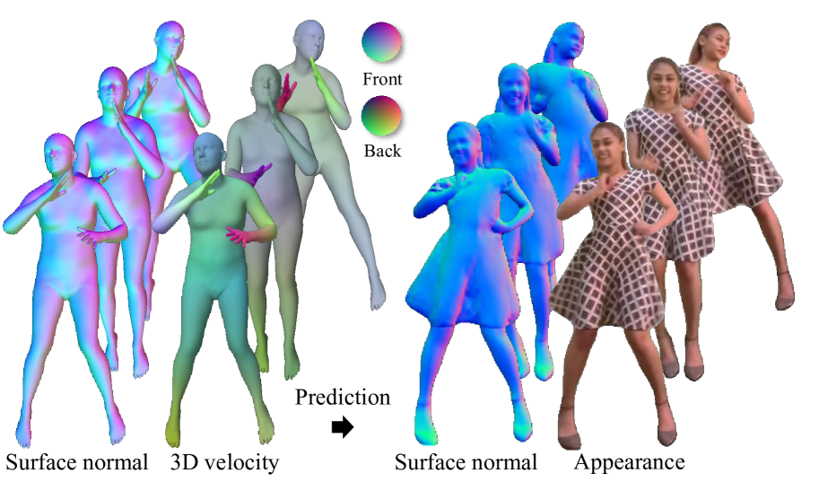
We express ourselves by moving our body that drives a sequence of natural secondary motion, e.g., dynamic movement of dress induced by dancing as shown in Figure 1. This secondary motion is the resultant of complex physical interactions with the body, which is, in general, time-varying. This presents a major challenge for plausible rendering of dynamic dressed humans in applications such as video based retargetting or social presence. Many existing approaches such as pose-guided person image generation [7] focus on static poses as a conditional variable. Despite its promising rendering quality, it fails to generate a physically plausible secondary motion, e.g., generating the same appearance for fast and slow motions.
One can learn the dynamics of the secondary motion from videos. This, however, requires a tremendous amount of data, i.e., videos depicting all possible poses and associated motions. In practice, only a short video clip is available, e.g., the maximum length of videos in social media (e.g., TikTok) are limited to 15-60 seconds. The learned representation is, therefore, prone to overfitting.
In this paper, we address the fundamental question of “can we learn a representation for dynamics given a limited amount of observations?”. We argue that a meaningful representation can be learned by enforcing an equivariant property—a representation is expected to be transformed in the way that the body pose is transformed. With the equivariance, we model the dynamics of the secondary motion as a function of spatial and time derivative of the 3D body. We construct this representation by re-arranging 3D features in the canonical coordinate system of the body surface, i.e., the UV map, which is invariant to the choice of the 3D coordinate system.
The UV map also captures the semantic meaning of body parts since each body part is represented by a UV patch. The resulting representation is compact and discriminative compared to the 2D pose representations that often suffer from geometric ambiguity due to 2D projection.
We observe that two dominant factors significantly impact the physicality of the generated appearance. First, the silhouette of dressed humans is transformed according to the body movement and the physical properties (e.g., material) of the individual garment types (e.g., top and bottom garments might undergo different deformations). Second, the local geometry of the body and clothes is highly correlated, e.g., surface normals of T-shirt and body surface, which causes appearance and disappearance of folds and wrinkles. To incorporate these factors, we propose a compositional decoder that breaks down the final appearance rendering into modular subtasks. This decoder predicts the time-varying semantic maps and surface normals as intermediate representations. While the semantic maps capture the time-varying silhouette deformations, the surface normals are effective in synthesizing high quality textures, which further enables re-lighting. We combine these intermediate representations to produce the final appearance.
Our experiments show that our method can generate a temporally coherent video of an unseen secondary motion from novel views given a single view training video. We conduct thorough comparisons with various state-of-the-art baseline approaches. Thanks to the discriminative power, our representation demonstrates superior generalization ability, consistently outperforming previous methods when trained on shorter training videos. Furthermore, our method shows better performance in handling complex motion sequences including 3D rotations as well as rendering consistent views in applications such as free-viewpoint rendering. The intermediate representations predicted by our method such as surface normals also enable applications such as relighting which are otherwise not applicable.
2 Related Work
Two major rendering approaches have been used for high quality human synthesis: model based and retrieval based approaches. Model based approaches leverage the 3D shape models, e.g., 3DMM face model [4], that can synthesize a novel view based on the geometric transformation [58, 11]. Retrieval approaches synthesize an image by finding matches in both local and global shape and appearance [6, 31]. These are, now, combined with a deep representation to form neural rendering and generative networks.
Neural Rendering. As human appearances are modulated by their poses, it is possible to generate the high fidelity appearance by using a parametric 3D body model, e.g., deformable template models [36]. For example, some existing approaches [45, 69] learned a constant appearance of a person by mapping from per-vertex RGB colors defined on the SMPL body to synthesized images. Textured neural avatars [52] learned a person-specific texture map by projecting the image features to a body surface coordinate (invariant to poses) to model human appearances. These approaches, however, are limited to statics, i.e., the generated appearance is completely blind to pose and motion.
To model pose-dependent appearances, Liu et al. [35] implicitly learned the texture variation over poses, which allowed them to refine the initial appearance obtained from texture map through a template model. On the other hand, Raj et al. [48] explicitly learned pose-dependent neural textures. To further enhance the quality of rendering, person-specific template models [2] were used by incorporating additional meshes representing the garments [66]. However, none of these approaches are capable of modeling the time-varying secondary motion. Habermann et al. [19] utilized a motion cue to model the motion-dependent appearances while requiring a pre-learned person-specific 3D template model. Zhang et al. [70] proposed a neural rendering approach to synthesize the dynamic appearance of loose garments assuming a coarse 3D garment proxy is provided. In contrast, our method uses the 3D body prior to model the dynamic appearance of both tight and loose garments.
The requirement of the parametric model can be relaxed by leveraging flexible neural rendering fields. For instance, neural volumetric representations [40] have been used to model general dynamic scenes [57, 65, 15, 59, 33] and humans [42, 43] using deformation fields. Nonetheless, the range of generated motion is still limited. Recent methods learned the appearance of a person in the canonical space of the coarse 3D body template and employ skinning and volume rendering approaches to synthesize images [47, 44, 8]. Liu et al. [34] extended such approaches by introducing pose-dependent texture maps to model pose-dependent appearance. Modeling time-varying appearance induced by the secondary motion with such volumetric approaches is still the uncharted area of study.
Generative Networks. Generative adversarial learning enforces a generator to synthesize photorealistic images that are almost indistinguishable from the real images. For example, image-to-image translation can synthesize pose-conditioned appearance of a person by using various pose representations such as 2D keypoints [37, 13, 46, 72, 53, 56, 50], semantic labels [39, 55, 12, 3, 68, 20, 14], or dense surface coordinate parametrizations [41, 17, 51, 1]. Despite remarkable fidelity, these were built upon the 2D synthesis of static images at every frame, in general, failing to generate physically plausible secondary motion. To address this challenge, several works have utilized temporal cues either in training time [7] to enable temporally smooth results or as input signals [61, 60] to model motion-dependent appearances. Kappel et al. [25] modeled the pose-dependent appearances of loose garments conditioned on 2D keypoints by learning temporal coherence using a recurrent network. However, due to the nature of 2D pose representations, the physicality of the generated motion is limited, e.g., our experiments show that the method works well mostly for planar motions but is limited in expressing 3D rotations. Wang et al. [63] is the closest to our work, which maps a sequence of dense surface parameterization to motion features that are used to synthesize dynamic appearances using StyleGAN [26]. In contrast, our method is built on a new 3D motion representation which shows superior discriminative power, consistently outperforming [63] in terms of generalizing to unseen poses as demonstrated in our experiments.
3 Method
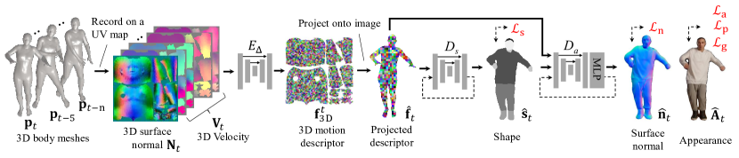
Given a monocular video of a person in motion and the corresponding 3D body fit estimates, we learn a motion representation to describe the time-varying appearance of the secondary motion induced by body movement (Section 3.1). We propose a multitask compositional renderer (Section 3.2) that uses this representation to render the subject-specific final appearance of moving dressed humans. Our renderer first predicts two intermediate representations including time-varying semantic maps that capture garment specific silhouette deformations and surface normals that capture the local geometric changes such as folds and wrinkles. These intermediate representations are combined to synthesize the final appearance. We obtain the 3D body fits estimates from the input video using a new model-based tracking optimization (Supplementary material). The overview of our rendering framework is shown in Figure 2.
3.1 Equivariant 3D Motion Descriptor
We cast the problem of human rendering as learning a representation via a feature encoder-decoder framework:
| (1) |
where an encoder takes as an input a representation of a posed body, (e.g., 2D sparse or dense keypoints or 3D body surface vertices), and outputs per-pixel features that can be used by the decoder to reconstruct the appearance of the corresponding pose where and are the width and height of the output image (appearance). We first discuss how can be modeled to render static appearance, then introduce our 3D motion descriptor to render time-varying appearance with secondary motion effects.
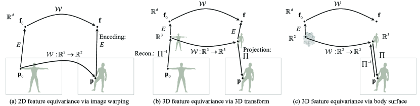
Learning a representation from Equation (1) from a limited amount of data is challenging because both encoder and decoder need to memorize every appearance in relation to the corresponding pose, . To address the data challenge, one can use an equivariant geometric transformation, , such that a feature is expected to be transformed in the way that the body pose is transformed:
| (2) |
where is an arbitrary pose. A naive encoder that satisfies this equiavariance learns a constant feature by warping any to a neutral pose :
| (3) |
where . Figure 3(a) and (b) illustrate cases where is defined as image warping in 2D or skinning in 3D respectively. can be derived by warping to the T-pose, of which feature can be warped back to the posed feature before decoding, . Since is constant, the encoder does not need to be learned. One can only learn the decoder to render a static appearance.
To model the time-varying appearance for the secondary motion that depends on both body pose and motion, one can extend Equation (3) to encode the spatial and temporal gradients as a residual feature encoding:
| (6) |
where and are the spatial and temporal derivatives of the posed body, respectively. The spatial derivatives essentially represent the pose corrective deformations [30, 36]. The temporal derivatives denote the body surface velocity which results in secondary motion. Since these spatial and temporal gradients are no longer constant, one needs to learn an encoder to encode the residual features.
In this paper, we use a 3D representation of the posed body lifted from an image by leveraging recent success in single view pose reconstruction [24, 9, 28]. Hence, spatial and temporal derivatives of the body pose correspond to the surface normals and body surface velocities, respectively:
| (7) |
where is the 3D surface normal, and represents the instantaneous velocities of the vertices in the body surface. We model the geometric transformation function to warp an arbitrary 3D pose to a canonical representation, . We record in a spatially aligned 2D positional map, specifically the UV map of the 3D body mesh where each pixel contains the 3D information of a unique point on the body mesh surface. This enables us to leverage 2D CNNs to apply local convolution operations to capture the relationship between neighboring body parts [38]. Therefore, called 3D motion descriptor is the feature defined in the UV coordinates where is the dimension of the per-vertex 3D feature. is the projected 3D feature in the image coordinates where is a coordinate transformation that transports the features defined in the UV space to the image plane via the dense UV coordinates of the body mesh.
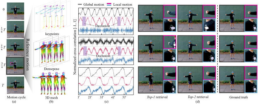
The key advantage of the 3D motion descriptor over commonly used 2D sparse [25] or dense [63] keypoint representations is discriminativity. Consider a toy example of a person rotating his body left to right multiple times. Given one cycle (i.e., 0-T) of such a motion as input (Figure 4(a)), assume we want to synthesize the appearance of the person performing the repetitions of the same motion (i.e., cycles T-5T). As a proof of concept, we model using a nearest neighbor classifier to retrieve the relevant image patches (top two patches) for each body part from the reference motion based on the correlation of the motion descriptors as shown in Figure 4(c). Due to the inherent depth ambiguity, multiple 3D motion trajectories yield the same 2D projected trajectory [23]. Hence, the 2D motion descriptors using sparse (Figure 4(b), top) and dense (Figure 4(b), middle) 2D keypoints confuse the directions of out-of-plane body rotation, resulting in erroneous nearest neighbor retrievals as shown in Figure 4(d). Furthermore, 2D representations entangle the viewpoint and pose into a common feature. This not only avoids a compact representation (e.g., the same body motion maps to different 2D trajectories with respect to different viewpoints and yields different features) but also suffers from occlusions in the image space. In our example in Figure 4(c), top and bottom, the upper arm is occluded in portions of the input video denoted with the purple blocks, hence no reliable local motion descriptors can be computed at those time instances. In contrast, our 3D motion descriptor is highly discriminative, which does not confuse the direction of body rotations, resulting in accurate image patch retrievals.
3.2 Multitask Compositional Decoder
Given 3D motion features, the decoder still needs to learn to generate diverse and plausible secondary motion, which is prone to overfitting given a limited amount of data. We integrate the following properties that can mitigate this challenge. (1) Composition: we design the decoder using a composition of modular functions where each modular function is learned to generate physically and semantically meaningful intermediate representations. Learning each modular function is more accurate than learning an end-to-end decoder as a whole as shown in our ablation study (Section 4.1); (2) Multi-task: each intermediate representation receives its own supervision signals resulting in multi-task learning. The motion features, , are shared by all intermediate modules resulting in a compact representation; (3) Recurrence: each module is modeled as an autoregressive network, which allows learning the dynamics rather than memorizing the pose-specific appearance.
Our decoder is a composition of two modular functions:
| (8) |
where and are the functions that generate the shape with semantic maps and the appearance.
learns the dynamics of the 2D shape:
| (9) |
where is the projected features onto the image at time , and is the predicted shape with semantics where is the number of semantic categories. In our experiments we set (background, top clothing, bottom clothing, face, hair, skin, shoes).
learns the dynamics of appearance given the shape and 3D motion descriptor:
| (10) |
where and are the generated appearance and surface normals at time .
We learn the 3D motion descriptor as well as the modular decoder functions by minimizing the following loss:
| (11) |
where , , , , are the appearance, shape, surface normal, perceptual similarity, and generative adversarial losses, and , , , and are their weights, respectively. We set , and in our experiments. is the training dataset composed of the ground truth 3D pose and its appearance .
where , , and are the generated appearance, shape, and surface normal, respectively. and are the shape [16] and surface normal estimates [22], and is the feature extractor that computes perceptual features from conv--2 layers in VGG-16 networks [54], is the PatchGAN discriminator [21] that validates the plausibility of the synthesized image conditioned on the shape mask.
3.3 Model-based Monocular 3D Pose Tracking
While there has been significant improvements in monocular 3D body estimation [28, 29, 9], we observe that predicting accurate and temporally coherent 3D body sequences is still challenging, which inhibit to reconstruct high-quality 3D motion descriptors. Hence, we devise a new optimization framework that learns a tracking function to address this challenge. We describe the full methodology and evaluation of our 3D tracking pipeline in the supplementary materials.
| Method | YouTube 1 (6K) | YouTube 2 (10K) | YouTube 3 (4K) | MPI (10K) | Custom 1 (15K) | Custom 2 (15K) | Avg. |
|---|---|---|---|---|---|---|---|
| EDN [7] | 0.954 / 3.06 / 0.356 | 0.943 / 4.39 / 0.465 | 0.871 / 6.23 / 0.467 | 0.824 / 4.59 / 0.287 | 0.916 / 5.26 / 0.450 | 0.928 / 5.06 / 0.423 | 0.906 / 4.76 / 0.408 |
| V2V [62] | 0.960 / 2.23 / 0.235 | 0.958 / 3.33 / 0.405 | 0.880 / 4.47 / 0.401 | 0.824 / 3.58 / 0.298 | 0.935 / 3.52 / 0.306 | 0.943 / 4.15 / 0.385 | 0.916 / 3.54 / 0.338 |
| HFMT [25] | 0.944 / 4.19 / 0.412 | 0.923 / 6.63 / 0.775 | 0.862 / 7.16 / 0.456 | 0.826 / 5.03 / 0.291 | 0.905 / 6.24 / 0.321 | 0.915 / 6.63 / 0.390 | 0.895 / 5.98 / 0.440 |
| DIW [63] | 0.966 / 2.21 / 0.275 | 0.960 / 3.03 / 0.370 | 0.894 / 4.69 / 0.396 | 0.825 / 2.94 / 0.359 | 0.939 / 3.23 / 0.304 | 0.944 / 3.95 / 0.412 | 0.921 / 3.34 / 0.336 |
| Ours | 0.973 / 2.01 / 0.240 | 0.964 / 2.83 / 0.338 | 0.897 / 4.50 / 0.412 | 0.825 / 2.82 / 0.203 | 0.942 / 3.12 / 0.279 | 0.946 / 3.81 / 0.404 | 0.925 / 3.18 / 0.312 |
4 Experiments
We validate the performance of our method across various examples and perform extensive qualitative and quantitative comparisons with previous work.
Implementation Details. We utilize the Adam optimizer [27] to train our model with a learning rate of . Given an input video ( frames), we train our model for roughly 72 hours using 4 NVIDIA V100 GPUs using a batch size of 4. Our motion features are learned from the body surface normals in the current frame and the body surface velocities in the past frames. The features are recorded in a UV map of size 128128. We synthesize final renderings and surface normal maps of size 512512. We implement our model in Pytoch and utilize the Pytorch3D differentiable rendering layers [49]. Details of the network designs and 3D tracking pipeline are given in the supplementary materials.
The coordinate transformation that transports the motion features from the UV space to the image plane, i.e., in Equation (7), can be implemented either by using image-based dense UV estimates [18] or by directly rendering the UV coordinates of the 3D body fits. To provide a fair comparison with previous work which also utilize dense UV estimates, we use the former option. When demonstrating our method on applications where we do not have corresponding ground truth frames to estimate dense UV maps (e.g., novel viewpoint synthesis), we use the latter option.
Baselines. We compare ours to four prior methods that focused on synthesizing dressed humans in motion. 1) Everybody dance now (EDN) [7] uses image-to-image translation to synthesize human appearance conditioned on 2D keypoints and uses a temporal discriminator to enforce plausible dynamic appearance. 2) Video-to-video translation (V2V) [62] is a sequential video generator that synthesizes high-quality human renderings from 2D keypoints and dense UV maps where the motion is modeled with optical flow in the image space. 3) High-fidelity motion transfer (HFMT) [25] is a compositional recurrent network which predicts plausible motion-dependent shape and appearance from 2D keypoints. 4) Dance in the wild (DIW) [63] synthesizes dynamic appearance of humans based on a motion descriptor composed of time-consecutive 2D keypoints and dense UV maps. We evaluate only on foreground by removing the background synthesized by the methods EDN, V2V, and DIW using a human segmentation method [16]. HFMT predicts a foreground mask similar to ours. In the supplementary material, we also compare our method to the 3D based approach [8] for neural avatar modeling from a single camera, which explicitly reconstruct the geometry of animatable human.
Datasets. We perform experiments on video sequences that demonstrate a wide range of motion sequences and clothing types, which include non-trivial secondary motion. Specifically, we select three dance videos (e.g., hip-hop and salsa) from YouTube and one sequence from prior work [25] that shows a female subject in a large dress. We also capture two custom sequences showing a male and a female subject respectively performing assorted motions (e.g., walking, running, punching, jumping etc.) including 3D rotations.
Metrics. We measure the quality of the synthesized frames with two metrics: 1) Structure similarity (SSIM) [64] compares the local patterns of pixel intensity in the normalized luminance and contrast space. 2) Perceptual distance (LPIPS) [71] evaluates the cognitive similarity of a synthesized image to ground truth by comparing their perceptual features extracted from a deep neural network. We evaluate the temporal plausibility by comparing the perceptual change across frames [10]: where and are the synthesized and ground truth images.
| Method | YouTube 1 (0.6K) | YouTube 2 (1K) | YouTube 3 (0.4K) | MPI (1K) | Custom 1 (1.5K) | Custom 2 (1.5K) | Avg. |
|---|---|---|---|---|---|---|---|
| DIW [63] | 0.939 / 4.12 / 0.330 | 0.940 / 5.00 / 0.463 | 0.869 / 6.75 / 0.513 | 0.824 / 4.45 / 0.472 | 0.915 / 5.46 / 0.566 | 0.920 / 6.36 / 0.698 | 0.901 / 5.36 / 0.507 |
| Ours | 0.949 / 3.36 / 0.457 | 0.951 / 4.16 / 0.402 | 0.883 / 5.35 / 0.546 | 0.824 / 4.09 / 0.327 | 0.928 / 4.25 / 0.512 | 0.931 / 4.95 / 0.558 | 0.911 / 4.36 / 0.467 |
4.1 Evaluation
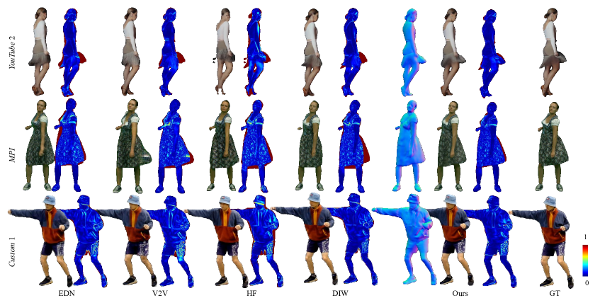
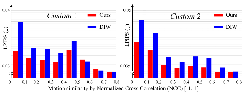
Comparisons We provide quantitative evaluation in Table 1 and show qualitative results in Figure 5 (see Supplementary Video). Similar to our method, we train each baseline for roughly 72 hours until convergence. Both qualitative and quantitative results show that sparse 2D keypoint based pose representation used in EDN is not as effective as other baselines or our method. HFMT is successful in modeling dynamic appearance changes for mostly planar motions (i.e., MPI sequence), but shows inferior performance in remaining sequences that involve 3D rotations. This is due to the depth ambiguity inherent in sparse 2D keypoint based representation. While V2V performs well in terms of quantitative numbers, it suffers from significant texture drifting issues as shown in Figure 5, second row. We speculate that this is due to the errors in the optical flow estimation, especially in case of loose clothing, which is used as a supervisory signal. DIW uses dense UV coordinates to model the dynamic appearance changes of loose garments and is the strongest baseline. While it performs consistently well, we observe that the performance gap between DIW and our method increases for motion segments consisting of 3D rotations. This gap is magnified when the testing motion deviates from the training data. In Figure 6, we plot how the perceptual error changes along the motion similarity between the training and testing data which is computed by NCC between two sets of the time-varying 3D meshes similar to Figure 4. We observe bigger increase in the error for DIW as testing frames deviate more from the training data.
We next perform further comparisons with DIW evaluating the generalization ability of each approach.
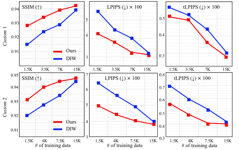
Generalization An effective motion representation that encodes the dynamic appearance change of dressed humans should be discriminative to distinguish all possible deformations induced by a pose transformation given the current state of the body and the garments. In order to compare the discriminative power of our motion descriptor and the dense keypoint based representation proposed by DIW, we evaluate how well each representation generalizes to unseen poses. Specifically, we train each model using only of the original training sequences by subsampling the training frames while ensuring training and testing pose sequences are sufficiently distinct. Considering the reduced amount of data, we limit the training time to 24 hours for both approaches. As shown in Table 2, the performance gap between the two methods increases. For the Custom 1 and 2 sequences, we further repeat the same experiment using , , and of the original training data as shown in Figure 7 where the performance of our method shows slower degradation than that of DIW. These quantitative results as well as visual results provided in the supplementary materials demonstrate the superiority of our 3D motion descriptor in terms of generalizing to novel poses.
Ablation Study Using the Custom 2 sequence, we train a variant w/o 3D motion descriptors by providing dense uv renderings as input directly to the decoder. We also disable the shape (w/o shape) and surface normal (w/o surface normal) prediction components. We repeat these trainings with subsampled data (). As shown in Table 3, the use of 3D motion descriptors and compositional rendering improves the perceptual quality of the synthesized images. The performance gap between our full model and w/o surface normal is larger with limited training data, implying that our multi-task framework helps with generalization. Qualitative results are given in the supplementary materials.
| Method | Full data (15K) | 10 data (1.5K) |
|---|---|---|
| w/o shape | 0.945 / 4.31 / 0.401 | 0.929 / 5.28/ 0.565 |
| w/o surface normal | 0.945 / 3.89 / 0.418 | 0.929 / 5.17 / 0.602 |
| w/o 3D motion | 0.942 / 4.17 / 0.584 | 0.928 / 5.43 / 0.760 |
| Full | 0.946 / 3.81 / 0.404 | 0.931 / 4.95 / 0.558 |
4.2 Applications
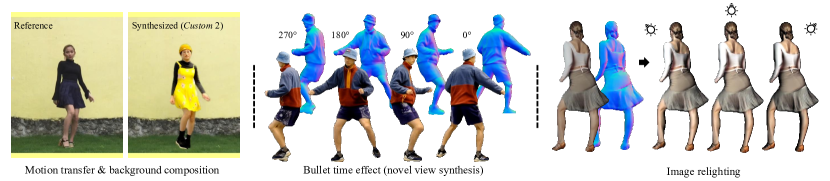
Our method enables several additional applications as shown in Figure 8. Since our method works with 3D body based motion representation, it can be easily used to transfer motion from a source to a target character by simply transferring the joint rotations between the characters. We can also create bullet time effects by creating a target motion sequence by globally rotating the 3D body. Thanks to the surface normal prediction, we can also perform relighting which is otherwise not applicable. Please refer to the supplementary material for more details and results.
5 Conclusion
We presented a method to render the dynamic appearance of a dressed human given a reference monocular video. Our method utilizes a novel 3D motion descriptor that encodes the time varying appearance of garments to model effects such as secondary motion. Our experiments show that our 3D motion descriptor is effective in modeling complex motion sequences involving 3D rotations. Our descriptor also demonstrates superior discriminator power compared to state-of-the-art alternatives enabling our method to better generalize to novel poses.
While showing impressive results, our method still has limitations. Highly articulated hand regions can appear blurry, hence refining the appearance of such regions with specialized modules is a promising direction. Our current model is subject specific, extending different parts of the model, e.g., 3D motion descriptor learning, to be universal is also an interesting future direction.
Broader Impact While our goal is to enable content creation for tasks such as video based motion retargeting or social presence, there can be some misuse of our technology to fabricate fake videos or news. We hope that parallel advances in deep face detection and image forensics can help to mitigate such concerns.
Acknowledgement
We would like to thank Julien Philip for providing useful feedback on our paper draft. Jae Shin Yoon is supported by Doctoral Dissertation Fellowship from University of Minnesota. This work is partially supported by NSF CNS-1919965.
References
- [1] Badour AlBahar, Jingwan Lu, Jimei Yang, Zhixin Shu, Eli Shechtman, and Jia-Bin Huang. Pose with Style: Detail-preserving pose-guided image synthesis with conditional stylegan. ACM Transactions on Graphics, 2021.
- [2] Timur Bagautdinov, Chenglei Wu, Tomas Simon, Fabian Prada, Takaaki Shiratori, Shih-En Wei, Weipeng Xu, Yaser Sheikh, and Jason Saragih. Driving-signal aware full-body avatars. SIGGRAPH, 2021.
- [3] Guha Balakrishnan, Amy Zhao, Adrian V Dalca, Fredo Durand, and John Guttag. Synthesizing images of humans in unseen poses. In CVPR, 2018.
- [4] Volker Blanz and Thomas Vetter. A morphable model for the synthesis of 3d faces. In SIGGRAPH, page 187–194, 1999.
- [5] Zhe Cao, Tomas Simon, Shih-En Wei, and Yaser Sheikh. Realtime multi-person 2d pose estimation using part affinity fields. In CVPR, 2017.
- [6] Dan Casas, Marco Volino, John Collomosse, and Adrian Hilton. 4d video textures for interactive character appearance. Comput. Graph. Forum, 33(2):371–380, May 2014.
- [7] Caroline Chan, Shiry Ginosar, Tinghui Zhou, and Alexei A Efros. Everybody dance now. In ICCV, 2019.
- [8] Jianchuan Chen, Ying Zhang, Di Kang, Xuefei Zhe, Linchao Bao, and Huchuan Lu. Animatable neural radiance fields from monocular rgb video. ICCV, 2021.
- [9] Vasileios Choutas, Georgios Pavlakos, Timo Bolkart, Dimitrios Tzionas, and Michael J Black. Monocular expressive body regression through body-driven attention. In ECCV, 2020.
- [10] Mengyu Chu, You Xie, Jonas Mayer, Laura Leal-Taixé, and Nils Thuerey. Learning temporal coherence via self-supervision for gan-based video generation. SIGGRAPH, 2020.
- [11] Alvaro Collet, Ming Chuang, Pat Sweeney, Don Gillett, Dennis Evseev, David Calabrese, Hugues Hoppe, Adam Kirk, and Steve Sullivan. High-quality streamable free-viewpoint video. ACM Trans. Graph., 34(4), July 2015.
- [12] Haoye Dong, Xiaodan Liang, Xiaohui Shen, Bochao Wang, Hanjiang Lai, Jia Zhu, Zhiting Hu, and Jian Yin. Towards multi-pose guided virtual try-on network. In ICCV, 2019.
- [13] Patrick Esser, Ekaterina Sutter, and Björn Ommer. A variational u-net for conditional appearance and shape generation. In CVPR, 2018.
- [14] Oran Gafni, Oron Ashual, and Lior Wolf. Single-shot freestyle dance reenactment. In CVPR, 2021.
- [15] Chen Gao, Ayush Saraf, Johannes Kopf, and Jia-Bin Huang. Dynamic view synthesis from dynamic monocular video. ICCV, 2021.
- [16] Ke Gong, Xiaodan Liang, Yicheng Li, Yimin Chen, Ming Yang, and Liang Lin. Instance-level human parsing via part grouping network. In ECCV, 2018.
- [17] Artur Grigorev, Artem Sevastopolsky, Alexander Vakhitov, and Victor Lempitsky. Coordinate-based texture inpainting for pose-guided human image generation. In Proceedings of the IEEE/CVF Conference on Computer Vision and Pattern Recognition, pages 12135–12144, 2019.
- [18] Rıza Alp Güler, Natalia Neverova, and Iasonas Kokkinos. Densepose: Dense human pose estimation in the wild. In CVPR, pages 7297–7306, 2018.
- [19] Marc Habermann, Lingjie Liu, Weipeng Xu, Michael Zollhoefer, Gerard Pons-Moll, and Christian Theobalt. Real-time deep dynamic characters. SIGGRAPH, 2021.
- [20] Xintong Han, Xiaojun Hu, Weilin Huang, and Matthew R Scott. Clothflow: A flow-based model for clothed person generation. In ICCV, 2019.
- [21] Phillip Isola, Jun-Yan Zhu, Tinghui Zhou, and Alexei A Efros. Image-to-image translation with conditional adversarial networks. In CVPR, 2017.
- [22] Yasamin Jafarian and Hyun Soo Park. Learning high fidelity depths of dressed humans by watching social media dance videos. In CVPR, pages 12753–12762, June 2021.
- [23] Eakta Jain, Yaser Sheikh, Moshe Mahler, and Jessica Hodgins. Augmenting Hand Animation with Three-dimensional Secondary Motion. In MZoran Popovic and Miguel Otaduy, editors, SCA. The Eurographics Association, 2010.
- [24] Angjoo Kanazawa, Michael J Black, David W Jacobs, and Jitendra Malik. End-to-end recovery of human shape and pose. In Proceedings of the IEEE conference on computer vision and pattern recognition, 2018.
- [25] Moritz Kappel, Vladislav Golyanik, Mohamed Elgharib, Jann-Ole Henningson, Hans-Peter Seidel, Susana Castillo, Christian Theobalt, and Marcus Magnor. High-fidelity neural human motion transfer from monocular video. In CVPR, 2021.
- [26] Tero Karras, Samuli Laine, and Timo Aila. A style-based generator architecture for generative adversarial networks. In CVPR, pages 4401–4410. Computer Vision Foundation / IEEE, 2019.
- [27] Diederik P Kingma and Max Welling. Auto-encoding variational bayes. ICLR, 2013.
- [28] Muhammed Kocabas, Nikos Athanasiou, and Michael J Black. Vibe: Video inference for human body pose and shape estimation. In CVPR, 2020.
- [29] Nikos Kolotouros, Georgios Pavlakos, Michael J Black, and Kostas Daniilidis. Learning to reconstruct 3d human pose and shape via model-fitting in the loop. In ICCV, 2019.
- [30] J. P. Lewis, Matt Cordner, and Nickson Fong. Pose space deformation: A unified approach to shape interpolation and skeleton-driven deformation. In SIGGRAPH, page 165–172, 2000.
- [31] Kun Li, Jingyu Yang, Leijie Liu, Ronan Boulic, Yu-Kun Lai, Yebin Liu, Yubin Li, and Eray Molla. Spa: Sparse photorealistic animation using a single rgb-d camera. IEEE Transactions on Circuits and Systems for Video Technology, 27(4):771–783, 2017.
- [32] Ruilong Li, Shan Yang, David A. Ross, and Angjoo Kanazawa. Ai choreographer: Music conditioned 3d dance generation with aist++, 2021.
- [33] Zhengqi Li, Simon Niklaus, Noah Snavely, and Oliver Wang. Neural scene flow fields for space-time view synthesis of dynamic scenes. In CVPR, 2021.
- [34] Lingjie Liu, Marc Habermann, Viktor Rudnev, Kripasindhu Sarkar, Jiatao Gu, and Christian Theobalt. Neural actor: Neural free-view synthesis of human actors with pose control. 2021.
- [35] Lingjie Liu, Weipeng Xu, Michael Zollhoefer, Hyeongwoo Kim, Florian Bernard, Marc Habermann, Wenping Wang, and Christian Theobalt. Neural rendering and reenactment of human actor videos. SIGGRAPH, 2019.
- [36] Matthew Loper, Naureen Mahmood, Javier Romero, Gerard Pons-Moll, and Michael J. Black. Smpl: A skinned multi-person linear model. ACM TOG, 2015.
- [37] Liqian Ma, Xu Jia, Qianru Sun, Bernt Schiele, Tinne Tuytelaars, and Luc Van Gool. Pose guided person image generation. In NeurIPS, 2017.
- [38] Qianli Ma, Shunsuke Saito, Jinlong Yang, Siyu Tang, and Michael J Black. Scale: Modeling clothed humans with a surface codec of articulated local elements. In CVPR, 2021.
- [39] Yifang Men, Yiming Mao, Yuning Jiang, Wei-Ying Ma, and Zhouhui Lian. Controllable person image synthesis with attribute-decomposed gan. In CVPR, 2020.
- [40] Ben Mildenhall, Pratul P. Srinivasan, Matthew Tancik, Jonathan T. Barron, Ravi Ramamoorthi, and Ren Ng. Nerf: Representing scenes as neural radiance fields for view synthesis. In ECCV, 2020.
- [41] Natalia Neverova, Riza Alp Guler, and Iasonas Kokkinos. Dense pose transfer. In ECCV, 2018.
- [42] Keunhong Park, Utkarsh Sinha, Jonathan T Barron, Sofien Bouaziz, Dan B Goldman, Steven M Seitz, and Ricardo Martin-Brualla. Deformable neural radiance fields. ICCV, 2021.
- [43] Keunhong Park, Utkarsh Sinha, Peter Hedman, Jonathan T Barron, Sofien Bouaziz, Dan B Goldman, Ricardo Martin-Brualla, and Steven M Seitz. Hypernerf: A higher-dimensional representation for topologically varying neural radiance fields. SIGGRAPH Asia, 2021.
- [44] Sida Peng, Junting Dong, Qianqian Wang, Shangzhan Zhang, Qing Shuai, Hujun Bao, and Xiaowei Zhou. Animatable neural radiance fields for human body modeling. In ICCV, 2021.
- [45] Sergey Prokudin, Michael J Black, and Javier Romero. Smplpix: Neural avatars from 3d human models. In WACV, 2021.
- [46] Albert Pumarola, Antonio Agudo, Alberto Sanfeliu, and Francesc Moreno-Noguer. Unsupervised person image synthesis in arbitrary poses. In CVPR, 2018.
- [47] Albert Pumarola, Enric Corona, Gerard Pons-Moll, and Francesc Moreno-Noguer. D-nerf: Neural radiance fields for dynamic scenes. In CVPR, 2021.
- [48] Amit Raj, Julian Tanke, James Hays, Minh Vo, Carsten Stoll, and Christoph Lassner. Anr: Articulated neural rendering for virtual avatars. In CVPR, year=2021.
- [49] Nikhila Ravi, Jeremy Reizenstein, David Novotny, Taylor Gordon, Wan-Yen Lo, Justin Johnson, and Georgia Gkioxari. Accelerating 3d deep learning with pytorch3d. arXiv:2007.08501, 2020.
- [50] Yurui Ren, Xiaoming Yu, Junming Chen, Thomas H Li, and Ge Li. Deep image spatial transformation for person image generation. In CVPR, 2020.
- [51] Kripasindhu Sarkar, Dushyant Mehta, Weipeng Xu, Vladislav Golyanik, and Christian Theobalt. Neural re-rendering of humans from a single image.
- [52] Aliaksandra Shysheya, Egor Zakharov, Kara-Ali Aliev, Renat Bashirov, Egor Burkov, Karim Iskakov, Aleksei Ivakhnenko, Yury Malkov, Igor Pasechnik, Dmitry Ulyanov, et al. Textured neural avatars. In CVPR, 2019.
- [53] Aliaksandr Siarohin, Stéphane Lathuilière, Sergey Tulyakov, Elisa Ricci, and Nicu Sebe. First order motion model for image animation. In NeurIPS, 2019.
- [54] Karen Simonyan and Andrew Zisserman. Very deep convolutional networks for large-scale image recognition. In International Conference on Learning Representations, 2015.
- [55] Sijie Song, Wei Zhang, Jiaying Liu, and Tao Mei. Unsupervised person image generation with semantic parsing transformation. In CVPR, 2019.
- [56] Hao Tang, Song Bai, Li Zhang, Philip HS Torr, and Nicu Sebe. Xinggan for person image generation. In European Conference on Computer Vision, 2020.
- [57] Edgar Tretschk, Ayush Tewari, Vladislav Golyanik, Michael Zollhöfer, Christoph Lassner, and Christian Theobalt. Non-rigid neural radiance fields: Reconstruction and novel view synthesis of a dynamic scene from monocular video. ICCV, 2021.
- [58] M. Volino, D. Casas, J.P. Collomosse, and A. Hilton. Optimal representation of multiple view video. In BMVC, 2014.
- [59] Chaoyang Wang, Ben Eckart, Simon Lucey, and Orazio Gallo. Neural trajectory fields for dynamic novel view synthesis. arXiv, 2021.
- [60] Ting-Chun Wang, Ming-Yu Liu, Andrew Tao, Guilin Liu, Jan Kautz, and Bryan Catanzaro. Few-shot video-to-video synthesis. NeurIPS, 2019.
- [61] Ting-Chun Wang, Ming-Yu Liu, Jun-Yan Zhu, Guilin Liu, Andrew Tao, Jan Kautz, and Bryan Catanzaro. Video-to-video synthesis. NeurIPS, 2018.
- [62] Ting-Chun Wang, Ming-Yu Liu, Jun-Yan Zhu, Andrew Tao, Jan Kautz, and Bryan Catanzaro. High-resolution image synthesis and semantic manipulation with conditional gans. In CVPR, 2018.
- [63] Tuanfeng Y. Wang, Duygu Ceylan, Krishna Kumar Singh, and Niloy J. Mitra. Dance in the wild: Monocular human animation with neural dynamic appearance synthesis, 2021.
- [64] Zhou Wang, Alan C Bovik, Hamid R Sheikh, and Eero P Simoncelli. Image quality assessment: from error visibility to structural similarity. TIP, 13(4):600–612, 2004.
- [65] Wenqi Xian, Jia-Bin Huang, Johannes Kopf, and Changil Kim. Space-time neural irradiance fields for free-viewpoint video. In CVPR, 2021.
- [66] Donglai Xiang, Fabian Andres Prada, Timur Bagautdinov, Weipeng Xu, Yuan Dong, He Wen, Jessica Hodgins, and Chenglei Wu. Explicit clothing modeling for an animatable full-body avatar. arXiv preprint arXiv:2106.14879, 2021.
- [67] Yuanlu Xu, Song-Chun Zhu, and Tony Tung. Denserac: Joint 3d pose and shape estimation by dense render-and-compare. In ICCV, pages 7759–7769, 2019.
- [68] Ceyuan Yang, Zhe Wang, Xinge Zhu, Chen Huang, Jianping Shi, and Dahua Lin. Pose guided human video generation. In ECCV, 2018.
- [69] Jae Shin Yoon, Lingjie Liu, Vladislav Golyanik, Kripasindhu Sarkar, Hyun Soo Park, and Christian Theobalt. Pose-guided human animation from a single image in the wild. In CVPR, 2021.
- [70] Meng Zhang, Tuanfeng Y. Wang, Duygu Ceylan, and Niloy J. Mitra. Dynamic neural garments. ACM TOG, 2021.
- [71] Richard Zhang, Phillip Isola, Alexei A Efros, Eli Shechtman, and Oliver Wang. The unreasonable effectiveness of deep features as a perceptual metric. In CVPR, 2018.
- [72] Zhen Zhu, Tengteng Huang, Baoguang Shi, Miao Yu, Bofei Wang, and Xiang Bai. Progressive pose attention transfer for person image generation. In CVPR, 2019.
In the supplementary materials, we provide the details and evaluations of our 3D performance tracking method, network designs for our human rendering models, and more results and comparison. Please also refer to the supplementary video.
A Model-based Monocular 3D Pose Tracking
Given a video of a moving person, we represent as the posed 3D body at each frame. Specifically, we predict the parameters of the template SMPL model [36], i.e., , where is a function that takes the pose and shape parameters and provides the vertex locations of the 3D posed body. To this end, we learn a tracking function that regresses accurate and temporally coherent pose and camera parameters from an image sequence:
| (12) |
where is the tracking function, is the image at time , and is the camera translation relative to the body, camera rotation is encoded in . We assume the shape, , is constant. We use a weak-perspective camera projection model [24] where we represent the camera translation in the z axis as the scale parameter. is learned by minimizing the following loss for each input video:
| (13) |
where , , , and are the fitting, rendering, data prior, and temporal consistency losses, respectively, and , , and are their weights. We set , and in our experiments. The overview of our optimization framework is described in Figure 9.
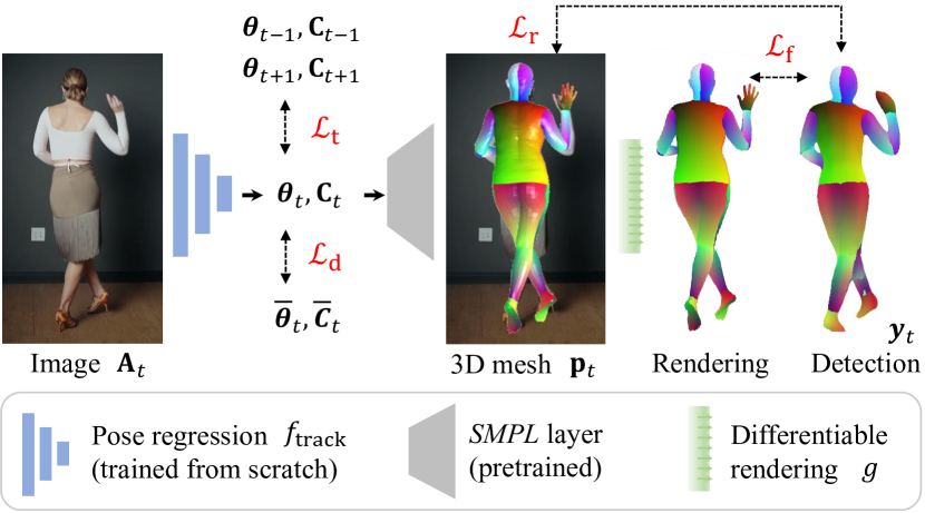
and utilize image-based dense UV map predictions [18] which enforce the 3D body fits to better align with the image space silhouettes of the body. Specifically, measures the 2D distance between the projected 3D vertex locations and corresponding 2D points in the image:
| (14) |
where is the set of dense keypoints in the image, obtained from image-based dense UV map predictions [67], are the corresponding 3D vertices, and is the camera projection which is a function of . measures the difference between the rendered and detected UV maps, :
| (15) |
where is the differentiable rendering function that renders the UV coordinates from the 3D body model.
provides the data driven prior on body and camera poses, i.e., , where and are the initial body and camera parameters predicted by a state-of-the-art method [28]. enforces the temporal smoothness over time: .
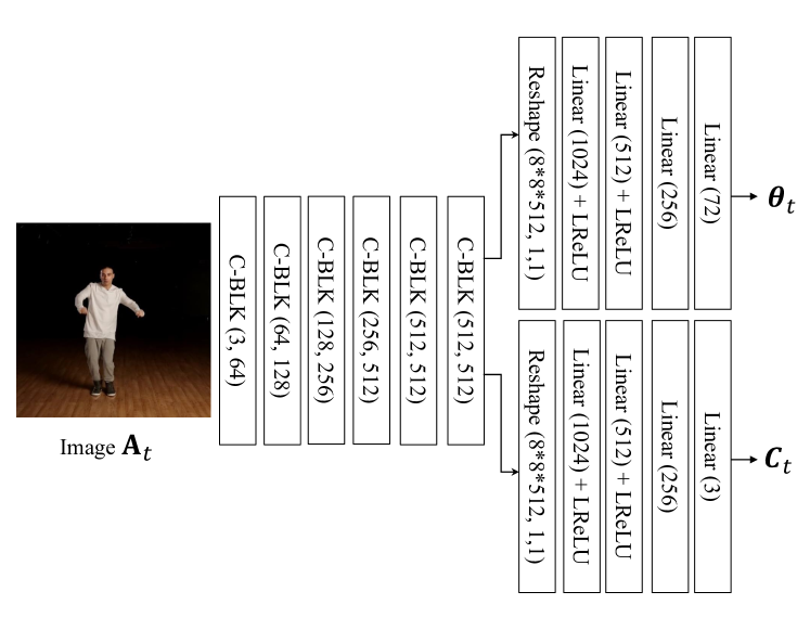
We enable using a convolutional neural network. The details of our network designs are described in Figure 10. where it predicts the 3D body and camera pose from an image .
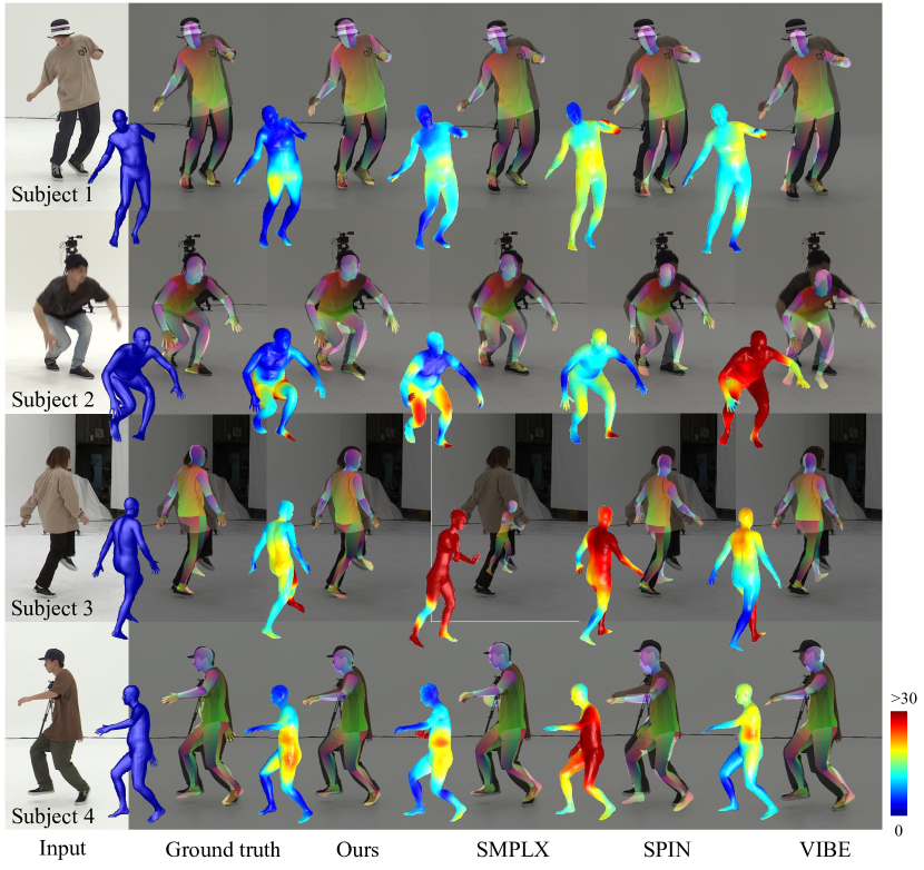
Evaluation We validate the performance of our 3D pose tracking method by comparing with previous monocular image based (SPIN [29] and SMPLx [9]) and video based (VIBE [28]) 3D body estimation methods.
We use the AIST++ dataset [32] which provides pseudo-ground truth SMPL fits obtained from multiview images. For randomly selected four subjects, we select four viewpoints and two motion styles (600 frames per motion) resulting in 4800 testing frames per subject. Due to the differences in the camera models adopted by each method (i.e., perspective or orthographic cameras), there exist a scale ambiguity between the predictions and the ground truth. Hence, we measure the per-vertex 2D projection error between the ground truth and predicted 3D body model in the image space. We provide quantitative and qualitative results in Table 4 and Figure 12, respectively. By exploiting both temporal cues and dense keypoint estimates, our method outperforms the previous work.
| Sub.1 | Sub.2 | Sub.3 | Sub.4 | Avg. | |
| SPIN [29] | 16.53.7 | 22.66.6 | 23.46.2 | 21.54.4 | 21.05.2 |
| VIBE [28] | 13.92.9 | 12.22.8 | 17.75.1 | 15.52.9 | 14.83.4 |
| SMPLx [9] | 9.01.6 | 10.21.7 | 16.210.2 | 12.14.4 | 11.94.5 |
| Ours | 8.31.1 | 8.72.0 | 13.73.5 | 11.31.9 | 10.52.1 |
B Comparison to 3D based Approach
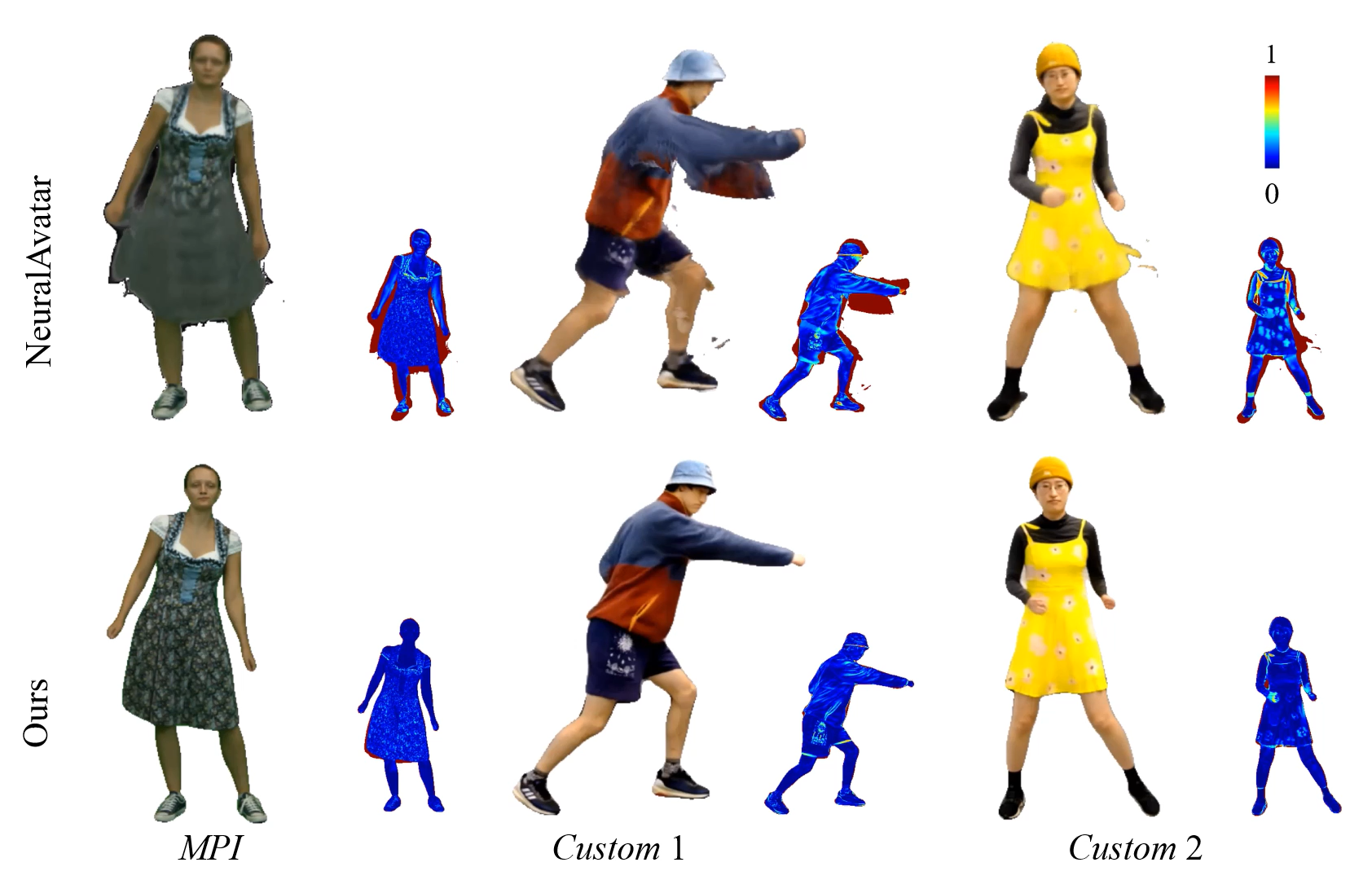
In Fig. 13 and Table 5, we show qualitative and quantitative comparisons to the recent 3D based method [8] for neural avatar modeling from a single camera, which explicitly reconstruct the geometry of animatable human. This method cannot effectively produce motion-dependent texture due to the failure in modeling of 3D deformation for clothing geometry, leading to rendering results with blurry, noisy, and static appearance as shown in Fig. 13, upper row.
| MPI | Custom 1 | Custom 2 | |
|---|---|---|---|
| NeuralAvatar [8] | 0.808 / 15.3 | 0.860 / 12.2 | 0.869 / 12.7 |
| Ours | 0.825 / 2.82 | 0.942 / 3.12 | 0.946 / 3.81 |
C More results
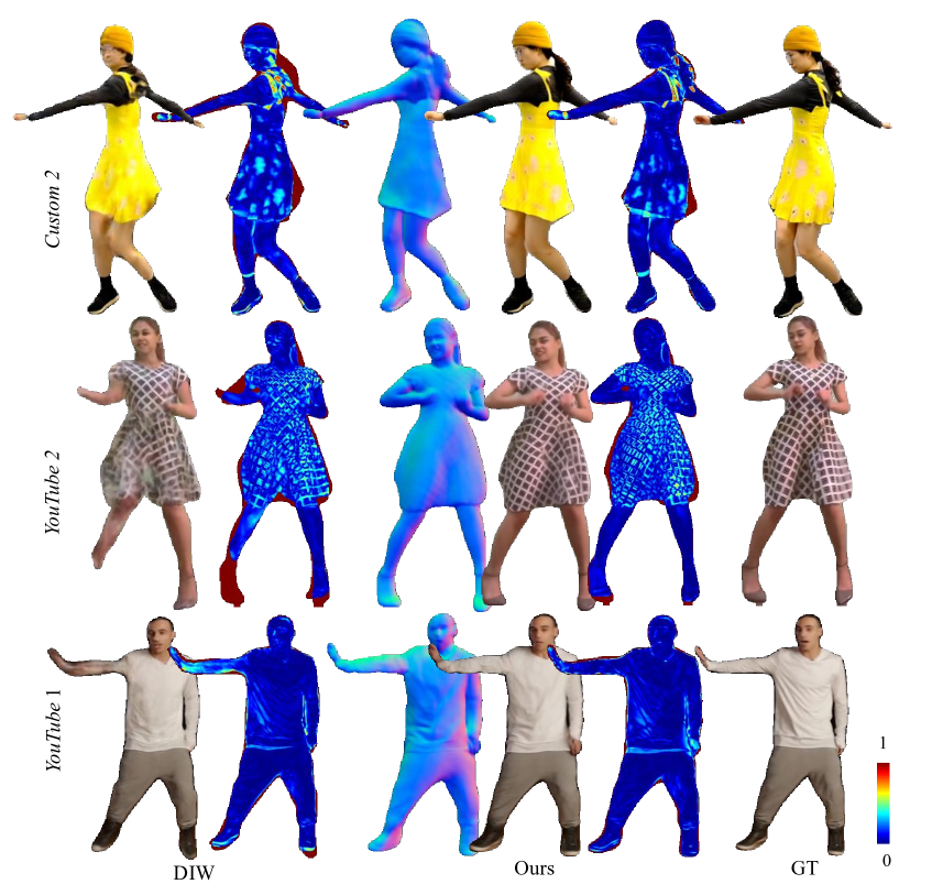
In Figure 14, we show the qualitative results of our rendering model and the one from DIW [63] which are trained with a small number of data (10 of the full training data). This result shows a similar trend as the Table 2 in the main manuscript.
D Network Designs for Human Rendering
We learn our motion encoder and compositional rendering decoders, using convolutional neural networks. In this section, we provide the implementation details of our network designs.
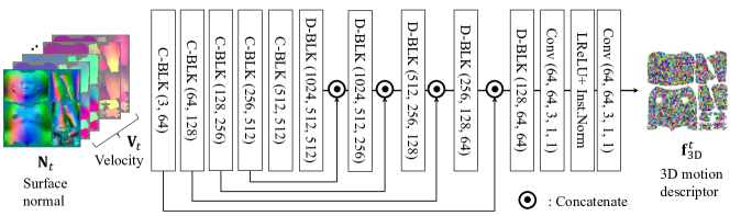
3D Motion Encoder Network, . Figure 15 describes the network details for our 3D motion encoder . It takes as input 3D surface normal of the current frame and velocity for past frames recorded in the UV space of the body and outputs 3D motion descriptors .
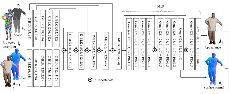
Shape Decoder Network, . Figure 16 describes the network details for our shape decoder network which takes as input the 3D motion descriptor rendered in the image space and the predicted shape in the previous time instance , and outputs the person-specific 2D shape which is composed seven category label maps.
Appearance Decoder Network, . Figure 17 describes the network details for our appearance decoder network which takes as input the projected 3D motion descriptor rendered in the image space, predicted shape , and the predicted appearance and surface normal in the previous time instance , and outputs the 3D surface normal and appearance .