Entanglement duality in spin-spin interactions

Abstract

We examine entanglement of thermal states for spin-$\frac{1}{2}$ dimers in external magnetic fields. Entanglement transition in the temperature-magnetic field plane demonstrates a duality in spin-spin interactions. This identifies dual categories of symmetric and anti-symmetric dimers with each category classified into toric entanglement classes. The entanglement transition line is preserved from each toric entanglement class to its dual toric class. The toric classification is an indication of topological nature of the entanglement.

I Introduction

The classification concept has been incorporated into different fields of studies ranging from biological systems to abstract topology, in order to categorize relevant objects based on shared characteristics. Scientific classification schemes have not only led to new discoveries of materials and resources, such as in the topological classification of matter chiu16 and of entangled quantum states johansson14 , but have also significantly helped to find the most efficient and robust approaches to technological advances.

One of the fundamental characteristics of quantum mechanics is the quantum correlation or the entanglement, which lies at the heart of the difference between the classical and quantum world einstein1935 ; schrodinger1935 ; bell1964 . It is widely believed to be much stronger than classical correlations and over the years has become a critically important resource for many applications in quantum technology including quantum computing, quantum cryptography, quantum communication, and hyper-sensitive measurements nielsen2010 . As a primary attribute of quantum mechanics, quantum entanglement is also much more involved with the foundations, predictions and interpretations of quantum phenomena. It is strongly linked to the concepts of quantum phase transition and quantum geometric phases osterloh2002 ; osborne2002 ; wei2005 ; orus2008 ; son2011 ; azimi-mousolou2013 . Nonetheless, the mysterious characteristics of the quantum entanglement still needs to be explored in-depth.

Here we use entanglement in terms of concurrence hill1997 ; wootters98 from a new perspective, i.e. classification, in order to analyze spin-spin interactions in dimers and classify them into entanglement classes. For this, we focus on the entanglement transition line for thermal state of the general traceless spin-pair model in the external parameter space specified by temperature and applied magnetic field. With this we categorize dimers into dual categories of symmetric and anti-symmetric dimers. Each category is classified into toric entanglement classes, where each class together with its dual are distinguished by the same entanglement transition line in temperature-magnetic field plane. As a nontrivial example, we introduce dual symmetric and anti-symmetric Heisenberg spin-pair interactions and specify their toric entanglement classes. We note that in Ref. arnesen01 , the entanglement between two spins in a one dimensional Heisenberg chain has also been studied as a function of temperature and external magnetic field, but not from the classification approach, which is the main concern here.

II General Model Hamiltonian

We start with the general traceless spin-pair model described by the Hamiltonian ($\hbar=1$ throughout the paper)

$$H(\omega,\mathbb{J})=\frac{\omega_{+}}{2}\sigma_{z}^{(1)}+\frac{\omega_{-}}{2}\sigma_{z}^{(2)}+\boldsymbol{\sigma}^{(1)}\cdot\mathbb{J}\boldsymbol{\sigma}^{(2)},$$ (1)

with the real-valued matrix

$$\mathbb{J}=\left(\begin{array}[]{ccc}J_{xx}&J_{xy}&0\\ J_{yx}&J_{yy}&0\\ 0&0&J_{zz}\end{array}\right),$$ (5)

where

$$J_{xx} = \frac{1}{2}(J+r),\ J_{yy}=\frac{1}{2}(J-r),$$

$$J_{xy} = \frac{1}{2}\left(K-D\right),\ J_{yx}=\frac{1}{2}\left(K+D\right),$$

$$\omega_{\pm} = \omega\pm\Delta.$$ (6)

This model accounts for a wide range of important spin-spin interaction systems, including Heisenberg ($J=J_{zz}$), Dzyaloshinskii–Moriya (D), and symmetric exchange ($K$), as well as XY anisotropy ($r$). It further allows for the spins to interact differently with the external magetic field ($\Delta$), due to field inhomogenties or differences in magnetic moments.

The two-qubit Hamiltonian is chosen so as to ensures that the thermal equilibrium state at temperature $T$ is of a $X$-type:

$$\varrho_{T}=\frac{1}{\mathcal{Z}}e^{-H/T}=\left(\begin{array}[]{cccc}\rho_{11}&0&0&\rho_{14}\\ 0&\rho_{22}&\rho_{23}&0\\ 0&\rho_{32}&\rho_{33}&0\\ \rho_{41}&0&0&\rho_{44}\end{array}\right).$$ (11)

in the ordered product qubit-qubit basis $\{|00\rangle,|01\rangle,|10\rangle,|11\rangle\}$ and we put Boltzmann’s constant $k_{B}=1$ from now. Explicitly, we have

$$\rho_{11} = \frac{1}{\mathcal{Z}}e^{-\frac{J_{zz}}{T}}[\cosh\frac{\epsilon_{1}}{T}-\sinh\frac{\epsilon_{1}}{T}\cos\vartheta],$$

$$\rho_{44} = \frac{1}{\mathcal{Z}}e^{-\frac{J_{zz}}{T}}[\cosh\frac{\epsilon_{1}}{T}+\sinh\frac{\epsilon_{1}}{T}\cos\vartheta],$$

$$\rho_{14} = \rho_{41}^{*}=-\frac{1}{\mathcal{Z}}e^{-\frac{J_{zz}}{T}}e^{-i\varphi}\sinh\frac{\epsilon_{1}}{T}\sin\vartheta,$$

$$\rho_{22} = \frac{1}{\mathcal{Z}}e^{\frac{J_{zz}}{T}}[\cosh\frac{\epsilon_{2}}{T}-\sinh\frac{\epsilon_{2}}{T}\cos\theta],$$

$$\rho_{33} = \frac{1}{\mathcal{Z}}e^{\frac{J_{zz}}{T}}[\cosh\frac{\epsilon_{2}}{T}+\sinh\frac{\epsilon_{2}}{T}\cos\theta],$$

$$\rho_{23} = \rho_{32}^{*}=-\frac{1}{\mathcal{Z}}e^{\frac{J_{zz}}{T}}e^{-i\phi}\sinh\frac{\epsilon_{2}}{T}\sin\theta,$$ (12)

where

$$\tan\vartheta = \frac{\sqrt{r^{2}+K^{2}}}{\omega},\ \ \ \ \ \ \ \ \tan\varphi=\frac{K}{r},$$ (13)

$$\tan\theta = \frac{\sqrt{J^{2}+D^{2}}}{\Delta},\ \ \ \ \ \ \ \ \tan\phi=\frac{D}{J},$$

$$\epsilon_{1} = \sqrt{\omega^{2}+r^{2}+K^{2}},\ \ \ \ \ \ \epsilon_{2}=\sqrt{\Delta^{2}+J^{2}+D^{2}},\ \$$

and $\mathcal{Z}=2\left(e^{-\frac{J_{zz}}{T}}\cosh\frac{\epsilon_{1}}{T}+e^{\frac{J_{zz}}{T}}\cosh\frac{\epsilon_{2}}{T}\right)$ the partition function.

The above $X$-state form is suitable in our analysis form two points of views: (i) as pointed out before, it accounts for thermal states of several important spin-spin interaction models, and (ii) the entanglement measure concurrence $C(\varrho_{T})$ hill1997 ; wootters98 can be calculated analytically. Indeed, one finds mazzola10

$$C(\varrho_{T})=2\max\big{\{}C_{1},C_{2},0\big{\}},$$ (14)

where

$$C_{1} = |\rho_{14}|-\sqrt{\rho_{22}\rho_{33}},$$

$$C_{2} = |\rho_{23}|-\sqrt{\rho_{11}\rho_{44}}.$$ (15)

We pursue by exploring the entanglement transition, for which one may solve

$$\max\big{\{}C_{1},C_{2}\big{\}}=0$$ (16)

to extract the critical line in the temperature-magnetic field parameter space. Eq. (16) gives rise to the following duality

$$(\text{I})\ \ \ \ \ C_{2}\leq C_{1} = 0$$

$$(\text{II})\ \ \ \ \ C_{1}\leq C_{2} = 0,$$ (17)

which becomes

$$(\text{I})\ \ \ \ \ e^{-\frac{2J_{zz}}{T}}p^{2}-e^{\frac{2J_{zz}}{T}}q^{2} = e^{\frac{2J_{zz}}{T}}$$

$$(\text{II})\ \ \ \ \ e^{\frac{2J_{zz}}{T}}q^{2}-e^{-\frac{2J_{zz}}{T}}p^{2} = e^{-\frac{2J_{zz}}{T}},$$ (18)

for our model system with $p=f(\epsilon_{1},\nu)$ and $q=f(\epsilon_{2},\theta)$ given by the function $f(x,y)=\sinh\frac{x}{T}\sin y$.

This duality equation allows us to categorize the spin-spin interactions in dimers into a dual categories of interactions. Here we focus on symmetric and antisymmetric dimers in the sense that the two spins of same size forming the dimer possess parallel or antiparallel orientations of the respective magnetic moments. For each case the corresponding Hamiltonian would have the following form

• Symmetric: Here with parallel magnetic moments we have $\omega_{+}=\omega_{-}=B$ and therefore

  $$H_{\text{s}} = \frac{B}{2}[\sigma_{z}^{(1)}+\sigma_{z}^{(2)}]+J_{zz}\sigma^{(1)}_{z}\sigma^{(2)}_{z}$$

  $$+\frac{J}{2}[\sigma^{(1)}_{x}\sigma^{(2)}_{x}+\sigma^{(1)}_{y}\sigma^{(2)}_{y}]-\frac{D}{2}[\sigma^{(1)}_{x}\sigma^{(2)}_{y}-\sigma^{(1)}_{y}\sigma^{(2)}_{x}]$$

  $$+\frac{r}{2}[\sigma^{(1)}_{x}\sigma^{(2)}_{x}-\sigma^{(1)}_{y}\sigma^{(2)}_{y}]+\frac{K}{2}[\sigma^{(1)}_{x}\sigma^{(2)}_{y}+\sigma^{(1)}_{y}\sigma^{(2)}_{x}].$$

  Note that we have $\Delta=0$ and $\theta=\pi/2$.

• Antisymmetric: In this case we have antiparallel magnetic moments, i.e., $\omega_{+}=-\omega_{-}=B$ and therefore

  $$H_{\text{as}} = \frac{B}{2}[\sigma_{z}^{(1)}-\sigma_{z}^{(2)}]-J_{zz}\sigma^{(1)}_{z}\sigma^{(2)}_{z}$$

  $$+\frac{J}{2}[\sigma^{(1)}_{x}\sigma^{(2)}_{x}+\sigma^{(1)}_{y}\sigma^{(2)}_{y}]-\frac{D}{2}[\sigma^{(1)}_{x}\sigma^{(2)}_{y}-\sigma^{(1)}_{y}\sigma^{(2)}_{x}]$$

  $$+\frac{r}{2}[\sigma^{(1)}_{x}\sigma^{(2)}_{x}-\sigma^{(1)}_{y}\sigma^{(2)}_{y}]+\frac{K}{2}[\sigma^{(1)}_{x}\sigma^{(2)}_{y}+\sigma^{(1)}_{y}\sigma^{(2)}_{x}],$$

  . (20)

  where in contrast to symmetric dimers we have $\omega=0$ and thus $\nu=\pi/2$.

We note that (I) and (II) in Eq. (18) classify the above two categories of symmetric and antisymmetric dimers, each within its own category, into equivalence classes of dimers in a way that all the dimers in the same class have the same entanglement phase diagram in the temperature-magnetic field parameter space. Explicitly, if we solve Eq. (18) for the critical line in the $(B,T)$ plane, across which the thermal state changes its entangling feature from entangled to separable, then we find out that two dimers specified with interaction parameters $(J,D,r,K)$ and $(J^{\prime},D^{\prime},r^{\prime},K)$ give rise to the same critical line in the $(B,T)$ plane or they are in the same class if and only if

$$\left\{\begin{array}[]{ll}J^{2}+D^{2}=J^{\prime 2}+D^{\prime 2}\\ r^{2}+K^{2}=r^{\prime 2}+K^{\prime 2}.\end{array}\right.$$ (23)

In other words, the above symmetric and antisymmetric categories consist of equivalence classes of dimers, where each class can be represented topologically as a two dimensional torus in the $(J,D,r,K)$ parameter space as shown in Fig. 1. Here, we may refer to an equivalence class of symmetric dimers as an S-class and an equivalence class of antisymmetric dimers as an AS-class.

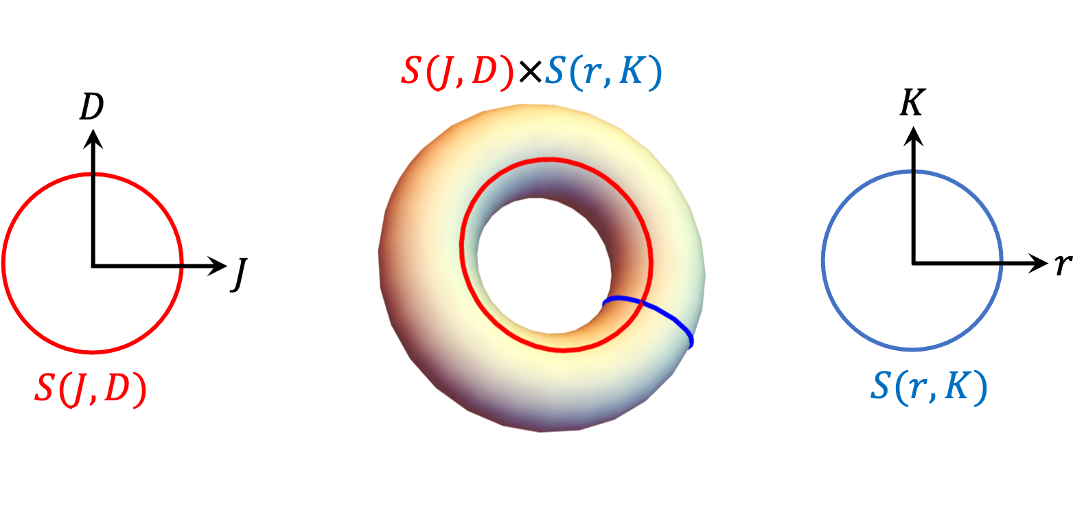
Figure 1: (Color online) Schematic picture of a S-class or AS-class as a two dimensional torus in the $(J,D,r,K)$ parameter space.

Having each category of dimers classified into equivalent toric classes of entangled spins, we further notice that each class in one category has its one-to-one correspondence dual class in the opposite category. To see this we realize that the two equations in the duality equation Eq. (18) are indeed two sides of the same coin and actually are related by flipping the sign of the $J_{zz}$ coupling parameter and exchanging the $p$ and $q$ functions. Therefore, if a given toric S-class characterized by the coupling parameters $(J,D,r,K)$ is obtained by one of the equations in Eq. (18), then its corresponding dual AS-class characterized by the coupling parameters $(\tilde{J},\tilde{D},\tilde{r},\tilde{K})$ can be obtained from the other equation in Eq. (18) and vice versa. The two dual toric S-class and AS-class are equivalent in a sense that they give rise to the same entanglement phase diagram in the $(B,T)$ plane if their characterisation parameters satisfy the following relations

$$\left\{\begin{array}[]{ll}J^{2}+D^{2}=\tilde{r}^{2}+\tilde{K}^{2}\\ r^{2}+K^{2}=\tilde{J}^{2}+\tilde{D}^{2}.\end{array}\right.$$ (26)

These relations compared to the ones given in Eq. (23) indicate that the dual symmetric and antisymmetric entanglement classes have the same toric characteristic but with their radial or meridian circles in swapped order as depicted in Fig 2.

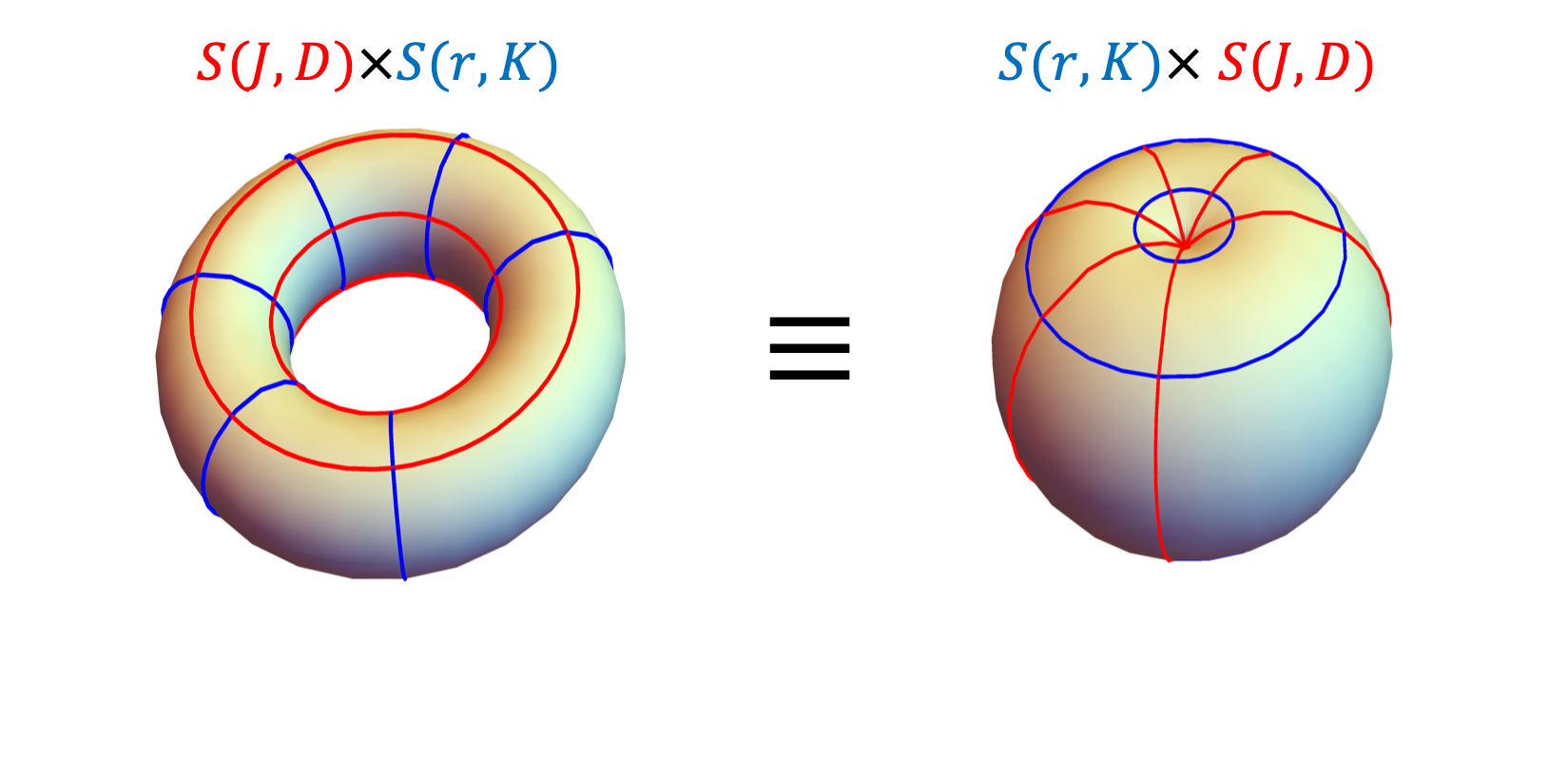
Figure 2: (Color online) Toric visualisation of dual symmetric and antisymmetric entanglement classes. Each class has the same toric characteristic as its dual but with radial or meridian circles in swapped order.

Note that although the above analysis focuses on concurrence, we have found exactly the same classification and entanglement duality using non-locality horodecki1995 ; horst13 and negativity Vidal2002 . Other than the entanglement duality in spin-spin interactions demonstrated above, our analysis reveals the geometric and topological nature of quantum entanglement in a sense that entanglement phase diagram in dimers provide a clear geometric foliation of coupling parameter manifold into two dimensional compact torus leaves.

To further clarify our point and show that the entanglement analysis above provide a non-trivial classification and duality, we consider two examples in the following section.

III Examples

Consider two identical spin-$\frac{1}{2}$ particles with Heisenberg spin-spin exchange interaction of strength $J$ in an external magnetic field, as given by the Hamiltonian

$$H^{\rm{Heisenberg}} = B\left(s_{z}^{(1)}+s_{z}^{(2)}\right)+J{\bf s}^{(1)}\cdot{\bf s}^{(2)}.$$ (27)

Here, ${\bf s}=\frac{1}{2}\boldsymbol{\sigma}$ and $B$ is the homogeneous field strength. We assume antiferromagnetic coupling $J>0$ as entanglement cannot occur for ferromagnetic coupling arnesen01 .

According to the above classification the Heisenberg model describes a class of symmetric dimers, which includes all the spin-spin interaction models following the general form of the Hamiltonian

$$H^{\rm{Heisenberg}}_{\text{s}} = B\left(s_{z}^{(1)}+s_{z}^{(2)}\right)+Js^{(1)}_{z}s^{(2)}_{z}$$

$$+J^{\prime}[s^{(1)}_{x}s^{(2)}_{x}+s^{(1)}_{y}s^{(2)}_{y}]$$

$$-D^{\prime}[s^{(1)}_{x}s^{(2)}_{y}-s^{(1)}_{y}s^{(2)}_{x}]$$

such that $J^{\prime 2}+D^{\prime 2}=J^{2}$. Note that $H^{\rm{Heisenberg}}_{\text{s}}=H_{\rm{Heisenberg}}$ for $D^{\prime}=0$ and $J^{\prime}=J$. Below we show all dimers in this class have the same entanglement phase diagram in $(B,T)$ plane.

For the Hamiltonian in Eq. (LABEL:eq:GHeisenberg), the thermal state is characterized by the following nonzero elements:

$$\rho^{\prime}_{11} = \frac{1}{\mathcal{Z}}e^{-B/T},\ \ \rho^{\prime}_{44}=\frac{1}{\mathcal{Z}^{\prime}}e^{B/T},$$

$$\rho^{\prime}_{22} = \rho^{\prime}_{33}=\frac{e^{J/2T}}{\mathcal{Z}^{\prime}}\cosh\left(\Gamma^{\prime}/2T\right),$$

$$\rho^{\prime}_{23} = (\rho^{\prime}_{32})^{\ast}=-\frac{e^{J/2T}}{\mathcal{Z}^{\prime}}e^{-i\phi}\sinh\left(\Gamma^{\prime}/2T\right)$$ (29)

with partition function

$$\mathcal{Z}^{\prime} = 2e^{J/2T}\cosh\left(\Gamma^{\prime}/2T\right)+2\cosh\left(B/T\right),$$ (30)

where $\Gamma^{\prime}=\sqrt{J^{\prime 2}+D^{\prime 2}}=J$. The concurrence functions are then given by

$$C_{1} = -\frac{e^{J/2T}}{\mathcal{Z}^{\prime}}\cosh\left(\Gamma^{\prime}/T\right)=-\frac{\left(1+e^{J/T}\right)}{2\mathcal{Z}^{\prime}}<0,$$

$$C_{2} = \frac{1}{\mathcal{Z}}\left[e^{J/2T}\sinh\left(\Gamma^{\prime}/T\right)-1\right]=\frac{e^{J/T}-3}{2\mathcal{Z}^{\prime}}$$ (31)

which result in

$$C(\varrho^{\prime}_{T})=\max\left\{\frac{e^{J/T}-3}{\mathcal{Z}^{\prime}},0\right\}.$$ (32)

Thus, $\varrho^{\prime}_{T}$ is entangled if $e^{J/T}-3>0$. This defines a critical temperature

$$T^{\prime}_{c}=\sqrt{J^{\prime 2}+D^{\prime 2}}/\ln 3=J/\ln 3\approx 0.91J,$$ (33)

which is independent of the external magnetic field $B$, for all dimers in the Heisenberg class denoted here by $[H^{\rm{Heisenberg}}]$. As shown in Fig. 3, above the critical temperature the thermal state ceases to be entangled. The same critical temperature as in Eq. (33) has been obtained in Ref. arnesen01 for antiferromagnetic Heisenberg exchange without the Dzyaloshinskii–Moriya interaction, i.e., $D^{\prime}=0$. Note that the toric characteristic equation

$$J^{\prime 2}+D^{\prime 2}=J^{2}$$ (34)

identifies each symmetric Heisenberg entanglement class as a one dimensional torus (one-sphere) in the $(J^{\prime},D)$ plane with the radius given by the strength of the Heisenberg coupling constant $J$. In other words, symmetric Heisenberg entanglement classes foliates the $(J^{\prime},D^{\prime})$ parameter space into circles (see Fig. 3).

On the opposite category of antisymmetric dimers, the dual Heisenberg model is described by the antisymmetric Hamiltonian

$$H^{\rm{Heisenberg}}_{\text{as}} = B\left(s_{z}^{(1)}-s_{z}^{(2)}\right)-Js^{(1)}_{z}s^{(2)}_{z}$$

$$+\tilde{r}[s^{(1)}_{x}s^{(2)}_{x}-s^{(1)}_{y}s^{(2)}_{y}]$$

$$+\tilde{K}[s^{(1)}_{x}s^{(2)}_{y}+s^{(1)}_{y}s^{(2)}_{x}],$$

(35)

where

$$\tilde{r}^{2}+\tilde{K}^{2}=J^{2}$$ (36)

with $J$ being the Heisenberg coupling constant in Eq. (27). In this case, the dual thermal state is given by the nonzero elements

$$\tilde{\rho}_{11} = \tilde{\rho}_{44}=\frac{e^{J/2T}}{\tilde{\mathcal{Z}}}\cosh\left(\tilde{\Gamma}/2T\right),$$

$$\tilde{\rho}_{22} = \frac{1}{\tilde{\mathcal{Z}}}e^{-B/T},\ \ \tilde{\rho}_{33}=\frac{1}{\tilde{\mathcal{Z}}}e^{B/T},$$

$$\tilde{\rho}_{14} = \tilde{\rho}_{41}^{\ast}=-\frac{e^{J/2T}}{\tilde{\mathcal{Z}}}e^{-i\varphi}\sinh\left(\tilde{\Gamma}/2T\right)$$ (37)

with partition function

$$\tilde{\mathcal{Z}} = 2e^{J/2T}\cosh\left(\tilde{\Gamma}/T\right)+2\cosh\left(B/T\right),$$ (38)

where $\tilde{\Gamma}=\sqrt{\tilde{r}^{2}+\tilde{K}^{2}}=J$. The concurrence functions are given by

$$C_{1} = \frac{1}{\tilde{\mathcal{Z}}}\left[e^{J/2T}\sinh\left(\tilde{\Gamma}/T\right)-1\right]=\frac{e^{J/T}-3}{2\tilde{\mathcal{Z}}},$$

$$C_{2} = -\frac{e^{J/2T}}{\tilde{\mathcal{Z}}}\cosh\left(\tilde{\Gamma}/T\right)=-\frac{\left(1+e^{J/T}\right)}{2\tilde{\mathcal{Z}}}<0,$$ (39)

which compared to its symmetric counterparts in Eq. (31) the $C_{1}$ and $C_{1}$ functions are swapped. This results in

$$C(\tilde{\varrho}_{T})=\max\left\{\frac{e^{J/T}-3}{\tilde{\mathcal{Z}}},0\right\}.$$ (40)

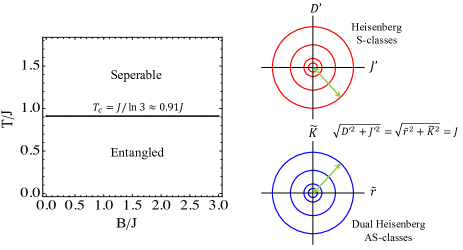
Figure 3: (Color online) Left panel shows the entanglement phase diagram for symmetric and dual antisymmetric Heisenberg dimers. For each of the Heisenberg type of dimers, the entanglement undergoes a sudden change at the relative critical temperature $T_{c}=T^{\prime}_{c}=\tilde{T_{c}}=J/\ln 3\approx 0.91J$ independent of the applied magnetic field strength $B$, which is an indication of quantum phase transition. Right panels illustrate toric visualisation of symmetric (S) and dual antisymmetric (AS) Heisenberg entanglement classes. While each circle of radius $J$ in the $(J^{\prime},D^{\prime})$ plane represent a Heisenberg S-class corresponding to a given isotropic Heisenberg exchange coupling $J$, the equivalent dual AS-class is represented by a circle in the $(\tilde{r},\tilde{K})$ plane with the same radius of $J$.

Similar to the symmetric Heisenberg dimers, the dual thermal state $\tilde{\varrho}_{T}$ is also entangled if $e^{J/T}-3>0$. This indicates the entanglement phase diagram with the critical temperature

$$\tilde{T}_{c}=\sqrt{\tilde{r}^{2}+\tilde{K}^{2}}/\ln 3=J/\ln 3\approx 0.91J,$$ (41)

for antisymmetric Heisenberg dimers to be the same as one obtained for symmetric Heisenberg dimers above. However, in the dual antisymmetric case the toric characteristic equation given by Eq. (36), as shown in Fig. 3 foliates instead the $(\tilde{r},\tilde{K})$ parameter space into circles of radii specified by the Heisenberg exchange parameter $J$.

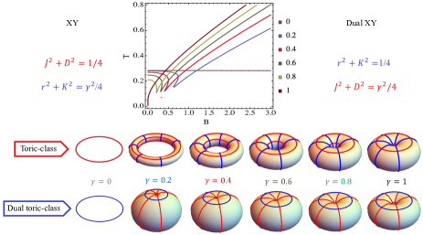
Figure 4: (Color online) Upper panel shows the entanglement transition curve for symmetric and dual antisymmetric XY dimers for different values of anisotropy parameter $\gamma$. While the isotropic limit $\gamma=0$ represents the narrowest area of entanglement with magnetic field independent critical temperature, the critical temperature becomes magnetic field dependent for $\gamma\neq 0$ and the entanglement area increases with $\gamma$ so that the Ising limit $\gamma=1$ represents the broadest entanglement area in the temperature-magnetic field plane. Each value of $\gamma$ distinguishes exclusive dual toric entanglement classes depicted in the lower panel.

In addition, Fig. 4 illustrates the classification of the XY interaction, given by the Hamiltonian

$$H^{\rm XY}_{\text{s/as}} = (1+\gamma)s_{x}^{(1)}s_{x}^{(2)}+(1-\gamma)s_{y}^{(1)}s_{y}^{(2)}$$ (42)

$$+B(s_{z}^{(1)}\pm s_{z}^{(2)}),$$

into dual toric entanglement classes. Here $\gamma\in[0,1]$ is the dimensionless anisotropy parameter controlling the cylindrical asymmetry of the spin-spin interaction and $+$ ($-$) is for symmetric (antisymmetric) XY model. The XY model defines interactions from the isotropic limit $\gamma=0$ with additional symmetry $[H^{\rm XY}_{\text{s/as}},s^{z}]=0$ to the opposite limit $\gamma=1$, which corresponds to the Ising model with totally ordered Neel ground state. By comparing the Hamiltonian in Eq. (42) with the dual symmetric and antisymmetric Hamiltonians in Eqs. (LABEL:SH) and (20) for $J_{zz}=0$ and then applying the above classification procedure to the XY model, we fine dual characteristic equations as

$$\left\{\begin{array}[]{ll}J^{2}+D^{2}=1/4\\ r^{2}+K^{2}=\gamma^{2}/4\end{array}\right.\equiv\left\{\begin{array}[]{ll}J^{2}+D^{2}=\gamma^{2}/4\\ r^{2}+K^{2}=1/4\end{array}\right.$$ (47)

which specify dual toric XY entanglement classes as depicted in the lower panel of Fig. 4. In fact, it is the anisotropy parameter $\gamma$ that controls the entanglement classes and the spin-spin duality. Note that the critical temperature depends on applied magnetic field for all $\gamma\neq 0$.

IV Conclusions

In conclusion, we have demonstrated an entanglement duality of a wide class of physically important spin-spin interaction dimer models by analyzing entanglement transition of thermal states in the temperature-magnetic field plane. This duality allows us to foliate coupling parameter space into dual symmetric and antisymmetric toric entanglement classes. This classification is an indication of topological nature of the quantum correlations and hope it can contribute to our deeper understanding of the various aspects of the mysterious concept of the quantum correlations.

V Acknowledgment

The authors acknowledge financial support from the Knut and Alice Wallenberg Foundation through Grant No. 2018.0060. E.S. acknowledges financial support from the Swedish Research Council (VR) through Grant No. 2017-03832.

References

• (1) C.-K. Chiu, J. C. Y. Teo, A. P. Schnyder, and S. Ryu, Classification of topological quantum matter with symmetries, Rev. Mod. Phys. 88, 035005 (2016).
• (2) M. Johansson, M. Ericsson, E. Sjöqvist, and A. Osterloh, Classification scheme of pure multipartite states based on topological phases, Phys. Rev. A 89, 012320 (2014).
• (3) A. Einstein, B. Podolsky, and N. Rosen, Can Quantum-Mechanical Description of Physical Reality Be Considered Complete?, Phys. Rev. 47, 777 (1935).
• (4) E. Schrödinger, The Present Status of Quantum Mechanics, Naturwissenschaften 23, 807 (1935).
• (5) J. S. Bell, On the Einstein Podolsky Rosen paradox, Physics 1, 195 (1964).
• (6) M. A. Nielsen and I. L. Chuang, Quantum Computation and Quantum Information, 10th Ed. (Cambridge University Press, Cambridge, England, 2010).
• (7) A. Osterloh, L. Amico, G. Falci, and R. Fazio, Scaling of entanglement close to a quantum phase transition, Nature (London) 416, 608 (2002).
• (8) T. J. Osborne and M. A. Nielsen, Entanglement in a simple quantum phase transition, Phys. Rev. A 66, 032110 (2002).
• (9) T.-C. Wei, D. Das, S. Mukhopadyay, S. Vishveshwara, and P. M. Goldbart, Global entanglement and quantum criticality in spin chains, Phys. Rev. A 71, 060305(R) (2005).
• (10) R. Orús, Universal Geometric Entanglement Close to Quantum Phase Transitions, Phys. Rev. Lett. 100, 130502 (2008).
• (11) W. Son, L. Amico, R. Fazio, A. Hamma, S. Pascazio, and V. Vedral, Quantum phase transition between cluster and antiferromagnetic states, Europhys. Lett. 95, 50001 (2011).
• (12) V. Azimi-Mousolou, C. M. Canali, and E. Sjöqvist, Unifying geometric entanglement and geometric phase in a quantum phase transition, Phys. Rev. A 88, 012310 (2013).
• (13) S. Hill and W. K. Wootters, Entanglement of a Pair of Quantum Bits, Phys. Rev. Lett. 78, 5022 (1997).
• (14) W. K. Wootters, Entanglement of Formation of an Arbitrary State of Two Qubits, Phys. Rev. Lett. 80, 2245 (1998).
• (15) M. C. Arnesen, S. Bose, and V. Vedral, Natural Thermal and Magnetic Entanglement in the 1D Heisenberg Model, Phys. Rev. Lett. 87, 017901 (2001).
• (16) L. Mazzola, B. Bellomo, R. Lo Franco, and G. Compagno, Connection among entanglement, mixedness, and nonlocality in a dynamical context, Phys. Rev. A 81, 052116 (2010).
• (17) R. Horodecki, P. Horodecki, and M. Horodecki, Violating Bell inequality by mixed spin-$\frac{1}{2}$ states: necessary and sufficient condition, Phys. Lett. A 200, 340 (1995).
• (18) B. Horst, K. Bartkiewicz, and A. Miranowicz, Two-qubit mixed states more entangled than pure states: Comparison of the relative entropy of entanglement for a given nonlocality, Phys. Rev. A 87, 042108 (2013).
• (19) G. Vidal and R. F. Werner, Computable measure of entanglement, Phys. Rev. A 65, 032314 (2002).