What to Hide from Your Students: Attention-Guided Masked Image Modeling

Abstract

Transformers and masked language modeling are quickly being adopted and explored in computer vision as vision transformers and masked image modeling (MIM). In this work, we argue that image token masking differs from token masking in text, due to the amount and correlation of tokens in an image. In particular, to generate a challenging pretext task for MIM, we advocate a shift from random masking to informed masking. We develop and exhibit this idea in the context of distillation-based MIM, where a teacher transformer encoder generates an attention map, which we use to guide masking for the student.

We thus introduce a novel masking strategy, called attention-guided masking (AttMask), and we demonstrate its effectiveness over random masking for dense distillation-based MIM as well as plain distillation-based self-supervised learning on classification tokens. We confirm that AttMask accelerates the learning process and improves the performance on a variety of downstream tasks. We provide the implementation code at https://github.com/gkakogeorgiou/attmask.

1 Introduction

Self-supervised learning (SSL) has attracted significant attention over the last years. Recently, several studies are shifting towards adapting SSL to transformer architectures. Originating in natural language processing, where self-supervised transformers [63, 15] have revolutionized the field, these architectures were introduced to computer vision with the vision transformer (ViT) [17] as an alternative to convolutional neural networks [35, 59, 26]. ViT formulates an image as a sequence of tokens obtained directly from raw patches and then follows a pure transformer architecture. Despite the absence of image-specific inductive bias, ViT shows strong image representation learning capacity.

Considering that transformers are data-hungry, many studies advocate pre-training them on unsupervised pretext tasks, determined only by raw data. A prominent paradigm is to mask a portion of the input tokens—words in text or patches in images—and train the transformer to predict these missing tokens [15, 2, 78, 24, 72]. This paradigm, called masked language modeling (MLM) in the language domain [15], is remarkably successful and extends to the vision domain as masked image modeling (MIM) [2, 72, 78].

MIM-based self-supervised methods have already shown impressive results on images. However, an important aspect that has not been well explored so far is how to choose which image tokens to mask. Typically, the selection is random, as has been the norm for text data. In this work, we argue that random token masking for image data is not as effective.

In text, random word masking is likely to hide high-level concepts that describe entire semantic entities such as objects (nouns) and actions (verbs). By contrast, an image has much more tokens than a sentence, which are highly redundant, and random masking is less likely to hide “interesting” parts; or when it does, the remaining parts still easily reveal the identity of the visual concepts. As shown in Figure 1(b-d), unless masking is very aggressive, this is thus less likely to form challenging token reconstruction examples that would allow the transformer to develop strong comprehension skills.

The question we ask is this: Can we develop a masking strategy that addresses this limitation and makes informed decisions on which tokens to mask?

To this end, we propose to exploit the intrinsic properties of ViT and in particular its self-attention mechanism. Given an input sequence of image patches, we forward it through the transformer encoder, thereby obtaining an attention map in its output. We then mask the most attended tokens. As shown in Figure 1(f-g), the motivation is that highly-attended tokens form more coherent image regions that correspond to more discriminative cues comparing with random tokens, thus leading to a more challenging MIM task.

This strategy, which we call attention-guided masking (AttMask), is an excellent fit to popular distillation-based self-supervised objectives, because it is the teacher encoder that sees the entire image and extracts the attention map, and the student encoder that sees the masked image and solves the reconstruction task. AttMask thus incurs zero additional cost.

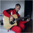
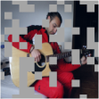
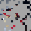
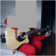
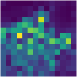
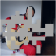
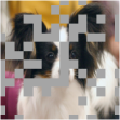
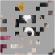
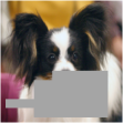
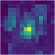
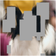
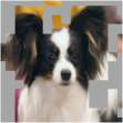
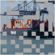
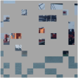
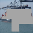
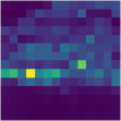
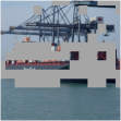
(a) Input	(b) Random	(c) Random	(d) Block	(e) Attention	(f) AttMask	(g) AttMask
Image	(30)	(75)	Wise	Map	High	Low

Figure 1: Different than random masking strategies (b-d), our attention-guided masking (AttMask) uses the attention map arising in the encoder (e) to mask the most highly attended by default (f), or the low-attended (g) patches. (b) is used by SimMIM [72], (c) by MAE [24], (d) by BEiT [2] and (g) by MST [38].

We make the following contributions:

1. We introduce a novel masking strategy for self-supervised learning, called AttMask, that exploits the intrinsic properties of ViT by leveraging its self-attention maps to guide token masking (subsection 3.2).

2. We show how to efficiently incorporate this above masking strategy into teacher-student frameworks that use a MIM reconstruction objective and demonstrate significant performance improvements over random masking.

3. Through extensive experimental evaluation, we confirm that AttMask offers several benefits: it accelerates the learning process; it improves performance on a data-limited regime (subsection 4.2) and on a variety of downstream tasks (subsection 4.3); it increases the robustness against background changes, thus revealing that it reduces background dependency.

2 Related Work

Vision Transformers.

Transformers are based on self-attention [63] and require pretraining on large unlabelled corpora [15]. Their adaptation to vision tasks is not straightforward. Representing pixels by tokens is impractical due to the quadratic complexity of self-attention, giving rise to approximations [11, 51, 67, 27, 65]. The idea of representing image patches by tokens is proposed in [13], where patches are of size $2\times 2$, and is further studied in ViT [17], where patches are $16\times 16$. Despite the absence of image-specific inductive bias, ViT is competitive to convolutional neural networks for ImageNet [14] and other smaller benchmark datasets [34, 46]. Since it is pretrained on a large and private dataset [58], authors of DeiT [62] question its efficiency and propose an improved data-efficient version, which however is based on a strong teacher instead [54].

Self-supervised Learning.

Early self-supervised learning methods follow the paradigm of training on an annotation-free pretext task, determined only by raw data [16, 22, 1, 36, 44, 48, 74, 32]. This task can be e.g. the prediction of patch orderings [48] or rotation angles [22]. Starting from instance discrimination [68] and contrastive predictive coding [50], contrastive learning has become very popular [9, 18, 3, 30, 43, 57, 66]. These methods pull positives together and push negatives apart, where positives are typically determined by different views of the same example. Alternatively, contrastive learning often relies on clustering [73, 5, 6, 7, 37, 79, 20]. The requirement of negatives is eliminated in BYOL [23], OBoW [21], SimSiam [10] and DINO [8], where the challenge is to avoid representation collapse, most notably by a form of self-distillation [60].

Using transformers, MIM as a pretext task is proposed in BEiT [2], which maps the images to discrete patch tokens and recovers tokens for masked patches, according to a block-wise random strategy. Other than that, MIM methods use continuous representations: SimMIM [72] randomly masks large patches and predicts the corresponding pixels by direct regression; MAE [24] randomly masks a large portion of patches and predicts the corresponding pixels using an autoencoder; MST [38] masks low-attended patches and reconstructs the entire input with a decoder; iBOT [78] extends the self-distillation loss of DINO to dense features corresponding to block-wise masked patches. Here, we advocate masking of highly-attended patches, in a sense the opposite of MST, and we exhibit this idea in the context of DINO and iBOT.

Regularization and Augmentation.

As the complexity of a task increases, networks with more and more parameters are introduced. But with increased representational power comes increased need for more data or risk of overfitting. Several regularization and data augmentation methods have been proposed in this direction [14, 55, 29, 56], combined with standard supervised tasks.

In this context, feature masking is introduced by Dropout [56], which randomly drops hidden neuron activations. To address the strong spatial correlation in convolutional feature maps, SpatialDropout [61] randomly drops entire channels. DropBlock [19] generalizes Dropout—or constrains SpatialDropout—by dropping features in a block, i.e., a square region of a feature map. Attention Dropout [12] makes use of self-attention to mask the most discriminative part of an image. Feature-space masking, guided by attention from another network or branch, has been extensively studied as a mechanism to explore beyond the most discriminative object parts for weakly-supervised object detection [31, 28, 75]. Our work is a natural evolution of these ideas, where attention is an intrinsic mechanism of transformers; and the task becomes that of densely reconstructing the masked features. This is a pretext task, without need for supervision.

3 Method

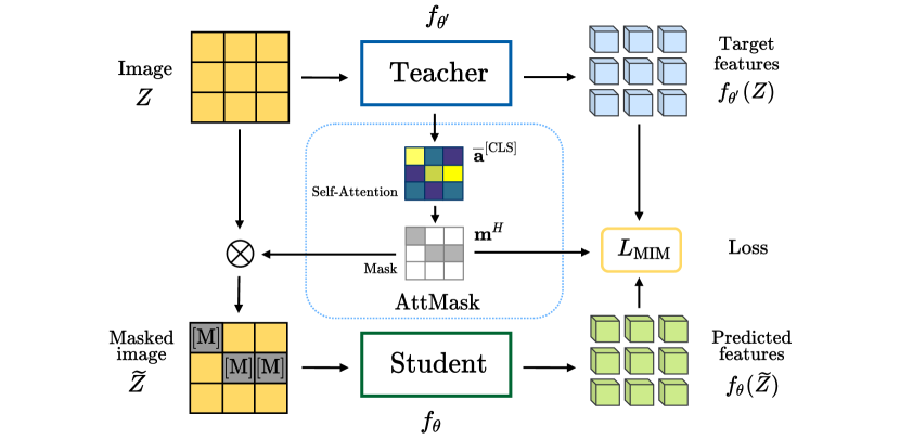
Figure 2: Simplified overview of AttMask as incorporated in the masked image modelling (MIM) objective of iBOT [78]. A tokenized image $Z$ (1) is given as input to a teacher encoder $f_{\theta^{\prime}}$, generating target features $f_{\theta^{\prime}}(Z)$ and an attention map $\overline{\mathbf{a}}^{\textsc{[cls]}}$ (7). We then generate a mask $\mathbf{m}^{H}$ (11) on the most attended tokens and accordingly a masked version $\widetilde{Z}$ (12) of the image, which is given as input to a student encoder $f_{\theta}$ to generate the predicted features $f_{\theta}(\widetilde{Z})$. Using $\mathbf{m}^{H}$, loss $L_{\textsc{MIM}}$ (3) is a dense distillation loss between predicted and target features of the masked tokens. Additionally, a global loss $L_{\textsc{g}}$ (4) between [cls] tokens is applied (not shown here).

A simplified overview of the method is shown in Figure 2. We first discuss in subsection 3.1 preliminaries and background on vision transformers and self-supervision with distillation-based masked image modeling. In subsection 3.2, we then detail our attention-guided token masking strategy, called AttMask, and how we incorporate it into masked image modeling.

3.1 Preliminaries and Background

Vision Transformer [17].

We are given an input image $X\in{}^{h\times w\times c}$, where $h\times w$ is the spatial resolution and $c$ is the number of channels. The first step is to tokenize it, i.e., convert it to a sequence of token embeddings. The image is divided into $n=hw/p^{2}$ non-overlapping patches $P_{i}\in{}^{p\times p\times c}$ for $i=1,\dots,n$, where $p\times p$ is the patch resolution. Each patch is flattened into a vector in ${}^{p^{2}c}$ and projected to an embedding vector $\mathbf{z}_{i}\in{}^{d}$ using a linear layer, where $d$ is the embedding dimension. A learnable embedding $\mathbf{z}^{\textsc{[cls]}}\in{}^{d}$ of a “classification” token [cls] is then prepended to form the tokenized image

$$Z=(\mathbf{z}^{\textsc{[cls]}};\mathbf{z}_{1};\dots;\mathbf{z}_{n})\in{}^{(n+1)\times d},$$ (1)

where “;” denotes row-wise stacking. The role of this special token is to represent the image at the output. A sequence of position embeddings is added to $Z$ to retain positional information. The resulting sequence is the input to the transformer encoder. Each layer of the encoder consists of a multi-head self-attention (MSA) block followed by a multi-layer perceptron (MLP) block. Through all of its layers, the encoder uses a sequence of fixed length $n+1$ of token embeddings of fixed dimension $d$, represented by a $(n+1)\times d$ matrix. The embedding of the [cls] token at the output layer serves as the image representation.

An MSA block consists of a number $H$ of heads, each computing a scaled dot-product self-attention [63], i.e., the relevance of each image patch to others, encoded as an $(n+1)\times(n+1)$ attention matrix. As discussed in subsection 3.2, we average attention matrices over all the heads of the last encoder layer and we use the row corresponding to the [cls] token to generate token masks.

Distillation-based Masked Image Modeling.

Self-distillation, using a moving average of the student as teacher [60], is studied for self-supervision in BYOL [23] and extended to vision transformers in DINO [8], which applies the distillation loss globally on the [cls] token. iBOT [78] turns this task into masked image modeling (MIM) by applying the loss densely on masked tokens.

Given an input image $X$ tokenized as $Z=(\mathbf{z}^{\textsc{[cls]}};\mathbf{z}_{1};\dots;\mathbf{z}_{n})$, a mask vector $\mathbf{m}=(m_{1},\dots,m_{n})\in\{0,1\}^{n}$ is generated, giving rise to a masked tokenized image $\widetilde{Z}=(\mathbf{z}^{\textsc{[cls]}};\tilde{\mathbf{z}}_{1};\dots;\tilde{\mathbf{z}}_{n})$, with

$$\tilde{\mathbf{z}}_{i}=(1-m_{i})\cdot\mathbf{z}_{i}+m_{i}\cdot\mathbf{z}^{\textsc{[mask]}}$$ (2)

for $i=1,\dots,n$, where $\mathbf{z}^{\textsc{[mask]}}\in{}^{d}$ is a learnable embedding of a “mask” token [mask]. Following the strategy of BEiT [2], the mask vector is generated with random block-wise token sampling, that is, defined in terms of random rectangles in the 2D layout of the $n$ tokens as a $(h/p)\times(w/p)$ matrix.

Following DINO [8], the transformer encoder is followed by a head that includes an MLP and scaled softmax, such that output token embeddings can be interpreted as probabilities. We denote by $f_{\theta}$ the mapping that includes the addition of the position embeddings, the encoder and the head, while $\theta$ is the set of learnable parameters. Given a tokenized image $Z$, masked or not, we denote by $f_{\theta}(Z)\in{}^{(n+1)\times d}$ the output token sequence and by $f_{\theta}(Z)_{i},f_{\theta}(Z)^{\textsc{[cls]}}\in{}^{d}$ the embedding of the $i$-th and [cls] token respectively. The teacher parameters $\theta^{\prime}$ are obtained from the student parameters $\theta$ by exponential moving average (EMA) according to $\theta^{\prime}\leftarrow\alpha\theta^{\prime}+(1-\alpha)\theta$.

For each input image, two standard resolution augmented global views are generated, with tokenized images $Z^{a},Z^{b}$ and mask vectors $\mathbf{m}^{a},\mathbf{m}^{b}$. For each view $v$ in $V=\{a,b\}$ and for each masked token, the MIM objective is to minimize the reconstruction loss between the student $f_{\theta}$ output for the masked input $\widetilde{Z}^{v}$ and the teacher $f_{\theta^{\prime}}$ output for the non-masked input $Z^{v}$:

$$L_{\textsc{mim}}=-\sum_{v\in V}\sum_{i=1}^{n}m_{i}^{v}f_{\theta^{\prime}}(Z^{v})_{i}\log({f_{\theta}(\widetilde{Z}^{v})_{i}}).$$ (3)

Following DINO [8], a similar loss is applied globally on the [cls] tokens between the student output for one masked view $\widetilde{Z}^{v}$ and the teacher output for the other non-masked view $Z^{u}$:

$$L_{\textsc{g}}=-\sum_{(u,v)\in V^{2}}\mathbbm{1}_{u\neq v}f_{\theta^{\prime}}(Z^{u})^{\textsc{[cls]}}\log(f_{\theta}(\widetilde{Z}^{v})^{\textsc{[cls]}}).$$ (4)

Finally, as detailed in the Appendix Appendix 0.B, a multi-crop strategy applies, giving rise to a loss $L_{\textsc{lc}}$ (A13) between local crops and global views. The overall loss of iBOT [78] is a weighted sum of $L_{\textsc{mim}}$ (3) and $L_{\textsc{g}}$ (4) $+$ $L_{\textsc{lc}}$ (A13). DINO itself uses the sum $L_{\textsc{g}}$ (4) $+$ $L_{\textsc{lc}}$ (A13) without masking.

3.2 AttMask: Attention-guided Token Masking

Prior MIM-based self-supervised methods use random or block-wise random token masking. In this section we describe our attention-guided token masking strategy, which hides tokens that correspond to the salient regions of an image and thus define a more challenging MIM objective.

Attention Map Generation.

Given an input sequence $Y\in{}^{(n+1)\times d}$, a multi-head self-attention (MSA) layer uses three linear layers to map $Y$ to the query $Q_{j}$, key $K_{j}$ and value $V_{j}$ sequences for $j=1,\dots,H$, where $H$ is the number of heads, $Q_{j},K_{j},V_{j}\in{}^{(n+1)\times d^{\prime}}$ and $d^{\prime}=d/H$. Then, it forms the $(n+1)\times(n+1)$ attention matrix, where softmax is row-wise:

$$A_{j}=\operatorname{softmax}\left(Q_{j}K_{j}^{\top}/\sqrt{d^{\prime}}\right).$$ (5)

To generate token masks from any layer of the transformer encoder, we average the attention matrices over all heads:

$$\overline{A}=\frac{1}{H}\sum_{j=1}^{H}A_{j}.$$ (6)

Now, each row of an attention matrix is a vector in ⁿ⁺¹, that corresponds to one token and, excluding the diagonal elements, determines an attention vector in ⁿ over all other tokens. We focus on the attention vector of the [cls] token, which comprises all but the first elements of the first row of $\overline{A}$:

$$\overline{\mathbf{a}}^{\textsc{[cls]}} =\left(\overline{a}_{1,2},\overline{a}_{1,3},\dots,\overline{a}_{1,n+1}\right),$$ (7)

where $\overline{a}_{i,j}$ is the element $i,j$ of $\overline{A}$. This vector can be reshaped to $(h/p)\times(w/p)$ attention map, to be visualized as a 2D image, indicating the regions of the input image that the [cls] token is attending.

Mask Generation: Highly-attended Tokens.

There is a permutation $\sigma_{\downarrow}:\{1,\dots,n\}\rightarrow\{1,\dots,n\}$ that brings the elements of $\overline{\mathbf{a}}^{\textsc{[cls]}}$ in descending order, such that $\overline{a}^{\textsc{[cls]}}_{\sigma_{\downarrow}(i)}\geq\overline{a}^{\textsc{[cls]}}_{\sigma_{\downarrow}(j)}$ for $i<j$, where $\overline{a}^{\textsc{[cls]}}_{i}$ is the $i$-th element of $\overline{\mathbf{a}}^{\textsc{[cls]}}$. Choosing a number $k=\left\lfloor{rn}\right\rfloor$ that is proportional to the total number $n$ of tokens with mask ratio $r\in[0,1]$, we define

$$M^{H}\coloneqq\{\sigma_{\downarrow}(i),\dots,\sigma_{\downarrow}(k)\}$$ (8)

as the set of indices of the top-$k$ most attended tokens. We thus define the high-attention mask vector $\mathbf{m}^{H}$ with elements

$$m_{i}^{H}\coloneqq\mathbbm{1}_{M^{H}}(i)=\left\{\begin{array}[]{cc}1&\quad\textrm{if}\ i\in M^{H}\\ 0&\quad\textrm{otherwise}\\ \end{array}\right.$$ (11)

for $i=1,\dots,n$. This masking strategy, which we call AttMask-High, essentially hides the patches that correspond to the most discriminative or salient regions of an image. By AttMask we shall refer to this strategy as default.

Low-attended Tokens.

We also examine the opposite approach of AttMask-High that masks the least attended tokens. In particular, we define the set of indices of the bottom-$k$ least attended tokens $M^{L}=\{\sigma_{\uparrow}(i),\dots,\sigma_{\uparrow}(k)\}$ and the low-attention mask vector $\mathbf{m}^{L}$ with $m_{i}^{L}\coloneqq\mathbbm{1}_{M^{L}}(i)$ based on the permutation $\sigma_{\uparrow}$ that brings the elements of $\overline{\mathbf{a}}^{\textsc{[cls]}}$ in ascending order, that is, $\overline{a}^{\textsc{[cls]}}_{\sigma_{\downarrow}(i)}\leq\overline{a}^{\textsc{[cls]}}_{\sigma_{\downarrow}(j)}$ for $i<j$. This strategy, which we call AttMask-Low and is similar to the masking strategy of MST [38], hides patches of the image background. Our experiments show that AttMask-Low does not work well with the considered MIM-based loss.

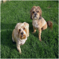
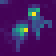
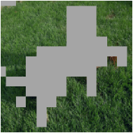
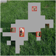
(a) Input Image	(b) Attention Map	(c) AttMask-High	(d) AttMask-Hint

Figure 3: Given image (a), the mean attention map (b) is averaged over heads (6),(7). The AttMask-High strategy (c) masks the most attended patches, while AttMask-Hint (d) reveals few of them to leave hints about the identity of the masked object.

Highly-attended with Hints.

Finally, because AttMask-High may be overly aggressive in hiding the foreground object of an image, especially when the mask ratio $r$ is high, we also examine an alternative strategy that we call AttMask-Hint: While still masking highly attended tokens, we allow a small number of the most highly attended ones to be revealed, so as to leave hints about the identity of the masked object. In particular, we remove from the initial set $M^{H}$ a small number $m=\left\lfloor{sn}\right\rfloor$ of tokens with show ratio $s<r$. These $m$ tokens are randomly selected from the $\left\lfloor{s_{\max}n}\right\rfloor$ most attended tokens in $M^{H}$, where $s_{\max}>s$. An example comparing AttMask-Hint with AttMask-High is illustrated in Figure 3.

Incorporating AttMask into Self-supervised Methods.

Because the embedding of the [cls] token at the output layer of the transformer encoder serves as the image representation, we generate token masks based on the attention vector precisely of the [cls] token of the output layer. In particular, given a global view tokenized as $Z^{v}=(\mathbf{z}^{\textsc{[cls]}};\mathbf{z}_{1};\dots;\mathbf{z}_{n})$, we obtain the attention vector $\overline{\mathbf{a}}^{\textsc{[cls]}}$ (7) and the corresponding high-attention mask vector $\mathbf{m}^{H}$ (11) at the output layer of the teacher. Then, similarly to (2), we give as input to the student the masked version $\widetilde{Z}^{v}=(\mathbf{z}^{\textsc{[cls]}};\tilde{\mathbf{z}}_{1};\dots;\tilde{\mathbf{z}}_{n})$ with

$$\tilde{\mathbf{z}}_{i}=(1-m_{i}^{H})\cdot\mathbf{z}_{i}+m_{i}^{H}\cdot\mathbf{z}^{\textsc{[mask]}}.$$ (12)

We argue that masking highly attended regions using $\mathbf{m}^{H}$ helps in learning powerful representations. In section 4, we also experiment with low-attended regions using $\mathbf{m}^{L}$, supporting further our argument.

AttMask can be incorporated into different methods to either replace the block-wise strategy of BEiT [2] or introduce masking. For iBOT [78], we use $\widetilde{Z}^{v}$ in $L_{\textsc{mim}}$ (3) and $L_{\textsc{g}}$ (4). For DINO [8], we introduce masking by using $\widetilde{Z}^{v}$ for global views in $L_{\textsc{g}}$ (4), but not for local crops in the $L_{\textsc{lc}}$ (A13) loss (see Appendix Appendix 0.B).

4 Experiments

4.1 Setup

Datasets and Evaluation Protocol.

We pretrain iBOT and DINO on 20% and 100% of the ImageNet-1k [14] training set. For 20%, we select the first 20% of training samples per class. We evaluate on ImageNet-1k validation set by $k$-NN or linear probing. For linear probing, we train a linear classifier on top of features using the same training protocol as in DINO [8]. With linear probing, we also validate robustness against background changes on ImageNet-9 (IN-9) [69]. For $k$-NN [68], we freeze the pretrained model and extract features of training images, then use a $k$-nearest neighbor classifier with $k=20$. We also perform the same $k$-NN experiment, now extracting features only from $\nu\in\{1,5,10,20\}$ examples per class. This task is more challenging and is similar to few-shot classification, only the test classes are the same as in representation learning.

We downstream to other tasks either with or without finetuning. We finetune on CIFAR10 [34], CIFAR100 [34] and Oxford Flowers [47] for image classification measuring accuracy; on COCO [39] for object detection and instance segmentation measuring mean average precision (mAP); and on ADE20K [77] for semantic segmentation measuring mean Intersection over Union (mIoU). Without finetuning, we extract features as with $k$-NN and we evaluate using dataset-specific evaluation protocol and metrics. We test on revisited $\mathcal{R}$Oxford and $\mathcal{R}$Paris [53] for image retrieval measuring mAP [53]; on Caltech-UCSD Birds (CUB200) [64], Stanford Cars (CARS196) [33], Stanford Online Products (SOP) [49] and In-Shop Clothing Retrieval (In-Shop) [41] for fine-grained classification measuring Recall@$k$ [45]; and on DAVIS 2017 [52] for video object segmentation measuring mean region similarity $\mathcal{J}_{m}$ and contour-based accuracy $\mathcal{F}_{m}$ [52].

In Appendix Appendix 0.A, we provide more benchmarks, visualizations and ablations.

Implementation Details.

As transformer encoder, we use ViT-S/16 [17]. The attention map (7) is generated from the last layer of the teacher encoder by default, i.e., layer 12. We mask the input with probability $p=0.5$, while the mask ratio $r$ is sampled uniformly as $r\sim U(a,b)$ with $[a,b]=[0.1,0.5]$ by default. For AttMask-Hint, we set $s_{\max}=0.1$ and the show ratio $s$ is sampled uniformly from $[s_{\max}a,s_{\max}b]=[0.01,0.05]$. Following [8, 78], we apply multi-crop [7] scheme, as detailed in Appendix Appendix 0.B. The overall loss of iBOT [78] is a weighted sum of $L_{\textsc{mim}}$ (3), with weight $\lambda$, and $L_{\textsc{g}}$ (4) $+$ $L_{\textsc{lc}}$ (A13) (DINO [8]), with weight 1, where $L_{\textsc{lc}}$ (A13) is the multi-crop loss. By default, $\lambda=1$. Hyperparameters are ablated in subsection 4.4. Training details are given in the Appendix Appendix 0.B.

4.2 Experimental Analysis

We provide an analysis on 20% of ImageNet-1k training samples, incorporating AttMask into distillation-based MIM [78] or self-distillation only [8]. We also provide results on robustness against background changes.

Masking Strategies: Distillation-based MIM.

We explore a number of masking strategies using distillation-based MIM, by incorporating AttMask into iBOT [78]. We compare AttMask with random block-wise masking [2], which is the default in iBOT, random patch masking with the same ratio, as well as with a more aggressive ratio, following MAE [24]. AttMask masks the most attended tokens (AttMask-High) by default, but we also consider the least attended (AttMask-Low) and the most attended with hints (AttMask-Hint).

Table 1: Different masking strategies for iBOT [78] pre-training on 20% of ImageNet. Top-1 accuracy for $k$-NN, linear probing on ImageNet validation set; fine-tuning on CIFAR10/100. $\dagger$: default iBOT masking strategy from BEiT [2]. $\ddagger$: aggressive random masking strategy from MAE [24].

iBOT Masking	Ratio (%)	ImageNet-1k		CIFAR10	CIFAR100
		$k$-NN	Linear	Fine-tuning
Random Block-Wise†	10-50	46.7	56.4	98.0	86.0
Random‡	75	47.3	55.5	97.7	85.5
Random	10-50	47.8	56.7	98.0	86.1
AttMask-Low (ours)	10-50	44.0	53.4	97.6	84.6
AttMask-Hint (ours)	10-50	49.5	57.5	98.1	86.6
AttMask-High (ours)	10-50	49.7	57.9	98.2	86.6

We evaluate performance using $k$-NN and linear probing evaluation protocol on the validation set, along with a fine-tuning evaluation on CIFAR10 and CIFAR100. As shown in Table 1, the AttMask-High outperforms all other masking strategies on all the evaluation metrics. In particular, AttMask-High achieves an improvement of +3.0% on $k$-NN and +1.5% on linear probing compared with the default iBOT strategy (random block-wise).

Interestingly, random patch masking outperforms the default iBOT strategy, while the more aggressive MAE-like strategy is inferior and AttMask-Low performs the lowest. Intuitively, this means that masking and reconstruction of non-salient regions does not provide a strong supervisory signal under a MIM objective. By contrast, our AttMask creates the more aggressive task of reconstructing the most salient regions and guides the model to explore the other regions. In this setup, AttMask-Hint is slightly lower than AttMask-High.

Table 2: Top-1 $k$-NN accuracy on ImageNet-1k validation for iBOT pre-training on different percentage (%) of ImageNet-1k. $\dagger$: default iBOT masking strategy from BEiT [2]. % ImageNet-1k 5 10 20 100 Random Block-Wise^† 15.7 31.9 46.7 71.5 AttMask-High (ours) 17.5 33.8 49.7 72.5 Figure 4: Top-1 $k$-NN accuracy on ImageNet-1k validation for iBOT training vs. training epoch on 20% ImageNet training set. $\dagger$: default iBOT masking strategy from BEiT [2].

Data and Training Efficiency.

Self-supervised methods on vision transformers typically require millions of images, which is very demanding in computational resources. We advocate that being effective on less data and fast training are good properties for a self-supervised method. In this direction, we assess efficiency on less data and training time, still with iBOT training. In Table 2 we observe that our AttMask-High consistently outperforms the default random block-wise masking strategy of iBOT at lower percentage of ImageNet-1k training set. In addition, in Table 2, AttMask-High achieves the same performance as random block-wise with 42% fewer training epochs.

Table 3: Top-1 $k$-NN accuracy on ImageNet-1k validation for DINO [8] pre-training on 20% of the ImageNet-1k training set using mask ratio of 10-50%. $\dagger$: default DINO.

No Masking†	Random	AttMask-Low	AttMask-Hint	AttMask-High
43.0	43.4	42.7	43.6	43.5

Masking Strategies: Self-distillation Only.

Here, we compare masking strategies using distillation only, without MIM reconstruction loss, by incorporating AttMask into DINO [8]. That is, we apply only the cross-view cross-entropy loss on the [cls] token (4). In Table 3, AttMask-High improves $k$-NN by +0.5 compared with the default DINO (no masking), while AttMask-Low is inferior. This reveals that AttMask is effective even without a MIM loss. Moreover, AttMask-Hint is slightly better than AttMask-High in this setting.

Table 4: Background robustness: Linear probing of iBOT model on IN-9 [69] and its variations, when pre-trained on 20% ImageNet-1k under different masking strategies. $\dagger$: default iBOT masking strategy from BEiT [2]. $\ddagger$: aggressive random masking.

iBOT Masking	Ratio (%)	OF	MS	MR	MN	NF	OBB	OBT	IN-9
Random Block-wise†	10-50	72.4	74.3	59.4	56.8	36.3	14.4	15.0	89.1
Random‡	75	73.1	73.8	58.8	55.9	35.6	13.7	14.5	87.9
Random	10-50	72.8	75.3	60.4	57.5	34.9	10.3	14.4	89.3
AttMask-Low (ours)	10-50	66.0	71.1	55.2	52.2	32.4	12.5	14.0	86.6
AttMask-Hint (ours)	10-50	74.4	75.9	61.7	58.3	39.6	16.7	15.7	89.6
AttMask-High (ours)	10-50	75.2	76.2	62.3	59.4	40.6	15.2	15.3	89.8

Robustness Against Background Changes.

Deep learning models tend to depend on image background. However, to generalize well, they should be robust against background changes and rather focus on foreground. To analyze this property, we use ImageNet-9 (IN-9) dataset [69], which includes nine coarse-grained classes with seven background/foreground variations. In four datasets, the background is altered: Only-FG (OF), Mixed-Same (MS), Mixed-Rand (MR), and Mixed-Next (MN). In another three, the foreground is masked: No-FG (NF), Only-BG-B (OBB), and Only-BG-T (OBT).

In Table 4, we evaluate the impact of background changes on IN-9 and its variations, training iBOT under different masking strategies. We observe that, except for O.BB. and O.BT, AttMask-High is the most robust. On OBB and OBT where the foreground object is completely missing, AttMask-Hint exploits slightly better the background correlations with the missing object.

In the Appendix subsection 0.A.3, we provide visualizations of attention maps in Figure A5 and masking examples in Figure A7.

4.3 Benchmark

We pre-train iBOT with AttMask-High and AttMask-Hint on 100% of ImageNet-1k and compare it with baseline iBOT and other distillation-based methods.

Table 5: Top-1 accuracy on ImageNet validation set. (a) $k$-NN and linear probing using the full ImageNet training set; (b) k-NN using only $\nu\in\{1,5,10,20\}$ examples per class. Pre-training on 100% ImageNet-1k for 100 epochs.

Method	(a) Full		(b) Few Examples
	$k$-NN	Linear	$\nu=1$	5	10	20
DINO [8]	70.9	74.6
MST [38]	72.1	75.0
iBOT [78]	71.5	74.4	32.9	47.6	52.5	56.4
iBOT+AttMask-High	72.5	75.7	37.1	51.3	55.7	59.1
iBOT+AttMask-Hint	72.8	76.1	37.6	52.2	56.4	59.6

ImageNet Classification.

As shown in Table 5(a), AttMask-High brings an improvement of 1% $k$-NN and 1.3% linear probing over baseline iBOT [78] and is better than prior methods. AttMask-High is thus effective for larger datasets too. Table 5(b) shows results of the more challenging task where only $\nu\in\{1,5,10,20\}$ training examples per class are used for the $k$-NN classifier. In this case, AttMask-High is very effective, improving the baseline iBOT masking strategy by 3-4%, demonstrating the quality of the learned representation. In this setup, AttMask-Hint offers a further small improvement over AttMask-High. For simplicity though, we use AttMask-High by default as AttMask.

More results are given in the Appendix. In particular, in Table A13, we provide results similar to Table 5 but with pre-training for 300 epochs. Also, in Table A14 we report further supervised finetuning on ImageNet-1k. In Table A10, we investigate the quality of the patch features by using global average pooling (GAP) rather than the [CLS] token embeddings. In Table A11, we study the effect of masking salient image parts at inference.

Table 6: Fine-tuning for image classification on CIFAR10 [34], CIFAR100 [34] and Oxford Flowers [47]; Object detection (AP^b, %) and instance segmentation (AP^m, %) on COCO [39]; and semantic segmentation on ADE20K [77] (mIoU, %). Models pre-trained on 100% ImageNet-1k training set for 100 epochs.

Method	CIFAR10	CIFAR100	Flowers	COCO		ADE20K
	Accuracy			APb	APm	mIoU
iBOT	98.8	89.5	96.8	48.2	41.8	44.9
iBOT+AttMask	98.8	90.1	97.7	48.8	42.0	45.3

Downstream Tasks with Fine-tuning.

We fine-tune the pre-trained models with iBOT and iBOT with AttMask for image classification on CIFAR10 [34], CIFAR100 [34] and Oxford Flowers [47], object detection and instance segmentation on COCO [39], and semantic segmentation on ADE20K [77]. In Table 6, we observe that AttMask brings small improvement on the baseline iBOT masking strategy on image classification fine-tuning in all cases. Furthermore, we observe that AttMask improves clearly the scores by 0.6% AP^b on object detection and 0.4% mIoU on semantic segmentation.

Table 7: Image retrieval (mAP, %) on (a) $\mathcal{R}$Oxford and (b) $\mathcal{R}$Paris [53] and video object segmentation (mean region similarity $\mathcal{J}_{m}$ and contour-based accuracy $\mathcal{F}_{m}$, %) on (c) DAVIS 2017 [52], without fine-tuning. Models pre-trained on 100% ImageNet-1k training set for 100 epochs.

Method	(a) $\mathcal{R}$Oxford		(b) $\mathcal{R}$Paris		(c) DAVIS 2017
	Medium	Hard	Medium	Hard	$(\mathcal{J}\&\mathcal{F})_{m}$	$\mathcal{J}_{m}$	$\mathcal{F}_{m}$
iBOT	31.0	11.7	56.2	28.9	60.5	59.5	61.4
iBOT+AttMask	33.5	12.1	59.0	31.5	62.1	60.6	63.5

Table 8: Fine-grained classification (R@$k$: Recall@$k$, %) [45] without fine-tuning. Models pre-trained on 100% ImageNet-1k training set for 100 epochs.

Method	CUB200			CARS196			SOP			In-Shop
	R@1	2	4	R@1	2	4	R@1	10	100	R@1	10	20
iBOT	51.4	63.8	75.0	35.6	46.0	56.3	57.4	72.2	84.0	39.1	61.9	68.2
iBOT+AttMask	57.2	69.4	80.3	39.8	50.4	61.4	59.0	73.9	85.4	40.7	63.7	70.3

Downstream Tasks without Fine-tuning.

Without finetuning, we use the pretrained models with iBOT and iBOT with AttMask to extract features as with $k$-NN and we evaluate using dataset-specific evaluation protocol and metrics. As shown in Table 7(a,b), AttMask is very effective on image retrieval, improving by 1-3% mAP the baseline iBOT masking strategy on $\mathcal{R}$Oxford and $\mathcal{R}$Paris [53], on both medium and hard protocols. More impressive the performance on fine-grained classification, improving by 2-6% R@1 on all datasets, as shown in Table 8. Finally, AttMask improves on video object segmentation on DAVIS 2017 [52] on all metrics, as shown in Table 7(c). These experiments are very important because they evaluate the quality of the pretrained features as they are, without fine-tuning and without even an additional layer, on datasets of different distribution than the pretraining set. AttMask improves performance by a larger margin in this type of tasks, compared with ImageNet.

In Table A12 in the Appendix, we additionally provide results for scene classification with linear probing on Places205 [76].

4.4 Ablation Study

We provide an ablation for the main choices and hyperparameters of our masking strategy and loss function, incorporating AttMask into iBOT [78] and pre-training on 20% of ImageNet-1k training samples. We provide additional ablations in the Appendix. In Table A15, we examine the MIM loss weight. In Table A16, we ablate both the masking strategy and the mask ratio $r$.

Table 9: AttMask $k$-NN top-1 accuracy on ImageNet-1k validation for iBOT pre-training on 20% of ImageNet-1k vs. (a) layer from which the attention map (7) is generated; (b) masking probability $p$ (using batch size 180); and (c) mask ratio $r$.

(a) Layer				(b) Masking Prob $p$					(c) Mask Ratio $r$ (%)
6	9	11	12	0	0.25	0.50	0.75	1	10-30	10-50	10-70	30
48.1	48.1	49.8	49.7	43.4	47.3	49.4	49.4	44.2	49.5	49.7	48.5	49.1

Layer for Attention Map Generation.

The attention map (7) is generated from the last layer of the teacher encoder by default, that is, layer 12 of ViT-S. In Table 9(a), we aim to understand the impact of other layer choices on AttMask. We observe that the deeper layers achieve the highest $k$-NN performance. Although layer 11 works slightly better, we keep the choice of layer 12 for simplicity, since layer 12 embeddings are used anyway in the loss function.

Masking Probability and Mask Ratio.

We mask the global views with probability $p=0.5$ by default. Table 9(b) reports on other choices and confirms that this choice is indeed best. Therefore, it is useful that student network sees both masked and non-masked images.

The mask ratio $r$ is sampled uniformly as $r\sim U(a,b)$ with $[a,b]=[0.1,0.5]$ by default. Table 9(c) shows the sensitivity of AttMask with respect to the upper bound $b$, along with a fixed ratio $r=0.3$. AttMask is relatively stable, with the default interval $[0.1,0.5]$ working best and the more aggressive choice $[0.1,0.7]$ worst. This is possibly due to the foreground objects being completely masked and confirms that masking the most attended patches is an effective strategy. The added variation around the fixed ratio $r=0.3$ is beneficial.

5 Conclusion

By leveraging the self-attention maps of ViT for guiding token masking, our AttMask is able to hide from the student network discriminative image cues and thus lead to more challenging self-supervised objectives. We empirically demonstrate that AttMask offers several benefits over random masking when used in self-supervised pre-training with masked image modeling. Notably, it accelerates the learning process, achieves superior performance on a variety of downstream tasks, and it increases the robustness against background changes, thus revealing that it reduces background dependency. The improvement is most pronounced in more challenging downstream settings, like using the pretrained features without any additional learning or finetuning, or working with limited data. This reveals the superior quality of the learned representation.

Acknowledgments.

We thank Shashanka Venkataramanan for his valuable contribution to certain experiments. This work was supported by computational time granted from GRNET in the Greek HPC facility ARIS under projects PR009017, PR011004 and PR012047 and by the HPC resources of GENCI-IDRIS in France under the 2021 grant AD011012884. NTUA thanks NVIDIA for the support with the donation of GPU hardware. This work has been supported by RAMONES and iToBos projects, funded by the EU Horizon 2020 research and innovation programme, under grants 101017808 and 965221, respectively.

Appendix 0.A More Experiments

We provide more benchmarks (subsection 0.A.1), more ablations (subsection 0.A.2), and more visualizations (subsection 0.A.3).

0.A.1 More Benchmarks

How Does AttMask Affect the Patch Features?

In contrast with the DINO objective that is applied only on the output [CLS] token embeddings, the MIM objective is directly applied to the output features of the patch tokens. Table A10 shows that using global average pooling (GAP) over patch features instead of the [CLS] token embeddings, AttMask outperforms baseline iBOT [78] by 9.0% $k$-NN accuracy. This indicates that AttMask leads to a more challenging MIM objective, which in turn forces the ViT to learn more discriminative patch features.

Table A10: $k$-NN top-1 accuracy on ImageNet-1k validation using global average pooling (GAP) over patch features vs. the [CLS] token embeddings. Models are pre-trained on 100% of ImageNet-1k for 100 epochs.

	CLS	GAP
iBOT	71.5	49.0
iBOT + AttMask	72.5	58.0
Gain	+1.0	+9.0

Table A11: Linear probing top-1 accuracy on a more challenging masked version of ImageNet-1k validation set. Salient parts are gradually masked using the attention maps of the official pre-trained DINO ViT-Base model and setting the corresponding masked pixel values to zero (black). Models pre-trained on 100% of ImageNet-1k for 100 epochs.

Mask Ratio (%)	0	10	30	50	70
iBOT	74.4	64.8	47.6	31.4	17.0
iBOT + AttMask	75.7	66.9	50.0	34.2	20.5
Gain	+1.3	+2.1	+2.4	+2.8	+3.5

Does AttMask Lead to Better Exploitation of Non-Salient Parts?

We examine the performance of the models pre-trained on 100% of ImageNet-1k on a more challenging ImageNet-1k validation set. In particular, we gradually mask the salient parts using the attention maps of the official pre-trained DINO ViT-Base model and setting the corresponding masked pixel values to zero. Our assumption is that a more robust model should be less sensitive when salient parts of an object are missing. In Table A11, we observe that as more parts of the images are hidden, a larger gain occurs by using AttMask with iBOT. This indicates that AttMask leads to less sensitive models that exploit better the non-salient parts or even background context.

Table A12: Scene classification measuring accuracy (%) using linear probing on Places205 [76]. Models pre-trained on 100% ImageNet-1k training set for 100 epochs.

	iBOT	iBOT+AttMask
Places205	55.9	56.7

Downstream Tasks using Linear Probing.

We experiment on scene classification on Places205 [76], measuring classification accuracy, using linear probing evaluation on models pre-trained on 100% of ImageNet-1k for 100 epochs. In Table A12, we observe that AttMask improves scores by 0.8% accuracy.

Table A13: Top-1 accuracy on ImageNet validation set. (a) $k$-NN and linear probing using the full ImageNet training set; (b) k-NN using only $\nu\in\{1,5,10,20\}$ examples per class. Pre-training on 100% ImageNet-1k for 300 epochs.

Method	(a) Full		(b) Few Examples
	$k$-NN	Linear	$\nu=1$	5	10	20
SimCLR [9]	-	69.0
BYOL [23]	66.6	71.4
MoBY [71]	-	72.8
DINO [8]	72.8	76.1
MST [38]	75.0	76.9
iBOT [78]	74.6	77.4	38.9	54.1	58.5	61.9
iBOT+AttMask (Ours)	75.0	77.5	40.4	55.5	59.9	63.1

Training for More Epochs.

We train iBOT with AttMask on 100% of ImageNet-1k for 300 epochs. AttMask not only accelerates the learning process and has better performance on data-limited regimes as explained in the main paper, but as we see in Table A13(a), even when trained for many epochs and with many data, it still brings an improvement of 0.4% $k$-NN and 0.1% linear probing over baseline iBOT [78]. Also, AttMask outperforms all other state-of-the-art frameworks on linear probing evaluation on ImageNet-1k validation set. We highlight that MST [38] employs an additional CNN decoder, while AttMask achieves improved linear probing performance with fewer learnable parameters.

We argue that the higher improvement of AttMask $k$-NN compared with linear probing indicates higher quality of learned embeddings, since linear probing amounts to supervised classification on higher-dimensional embeddings and on the same dataset that was used for self-supervised pre-training. To validate this, we experiment with a more challenging variant of $k$-NN where only $\nu\in\{1,5,10,20\}$ examples per class of the training set are used. Table A13(b) shows that using AttMask for self-supervised pre-training and then using only simple $k$-NN classifier with only one example per class, achieves an accuracy improvement of 1.5% compared with the default iBOT. This highlights the superiority of AttMask in low-shot learning regimes, which are of great practical interest.

Table A14: Top-1 accuracy on ImageNet validation set after supervised fine-tuning for 100 epochs on ImageNet-1k training set. Models pre-trained on 100% ImageNet-1k training set for 300 epochs.

	iBOT	iBOT+AttMask
Fine-tuning on ImageNet	81.1	81.3

Full fine-tuning on ImageNet-1k.

For iBOT and iBOT+AttMask pre-trained on ImageNet-1k for 300 epochs, we also experiment with further supervised fine-tuning on ImageNet-1k, training for 100 epochs. We report results in Table A14. AttMask improves iBOT by 0.2% (81.1% $\rightarrow$ 81.3%), providing a better network initialization for supervised finetuning.

0.A.2 More Ablations

Table A15: $k$-NN top-1 accuracy on ImageNet-1k validation vs. MIM Loss Weight $\lambda$, while the weight of DINO loss is fixed to 1. Pre-training on 20% of ImageNet-1k for 100 epochs.

MIM Loss Weight $\lambda$	0.0	0.5	1.0	2.0
iBOT	43.4	46.5	46.7	41.9
iBOT+AttMask	43.5	47.3	49.7	48.3
Gain	+0.1	+0.8	+3.0	+6.4

MIM Loss Weight.

The overall loss of iBOT [78] is a weighted sum of $L_{\textsc{mim}}$ (3), with weight $\lambda$, and $L_{\textsc{g}}$ (4) $+$ $L_{\textsc{lc}}$ (A13) (DINO), with weight 1. Table A15 shows that AttMask is superior to the default block-wise random masking of iBOT in all cases, while the default $\lambda=1$ works best for both and yields the greatest gain of $3\%$ $k$-NN accuracy for AttMask. In particular, increasing the weight of the MIM loss leads to a larger gain in $k$-NN accuracy. This shows that AttMask boosts the MIM task.

Table A16: AttMask-High vs. random masking strategies: $k$-NN top-1 accuracy on ImageNet-1k validation for iBOT pre-training on 20% of ImageNet-1k for different mask ratio $r$. $\dagger$: default iBOT masking strategy from BEiT [2].

Mask Ratio $r$ (%)	10-30	10-50	10-70	30
Random Block-Wise	46.5	46.7†	47.1	46.9
Random	47.6	47.8	47.8	48.2
AttMask-High	49.5	49.7	48.5	49.1

Masking strategy and mask ratio.

We ablate both the masking strategy (random block-wise, random or AttMask-High) and the mask ratio $r$ in Table A16. AttMask-High with 10-50 mask ratio gives the best results.

0.A.3 More Visualizations

Input Image
Block-Wise
AttMask

Figure A5: Multi-head attention maps from the last layer, training iBOT with the default block-wise strategy from BEiT [2] and with our AttMask. From the attention matrix (5) of each head, we extract the attention map of the [cls] token and display in different color per head the patch tokens that are included in the top 60% of the attention mass.

Visualization of Attention Maps.

In Figure A5, we utilized the pre-trained models on 20% of ImageNet and observe that, when training iBOT with the default block-wise random masking strategy, there is at least one head (in blue) that attends the background to a great extent. By contrast, with our AttMask, all heads mostly attend salient objects or object parts. It appears that by focusing on reconstructing highly-attended masked tokens, the network learns to focus more on foreground objects.

	10%	30%	50%			10%	30%	50%
Block-Wise
Random
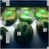
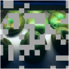
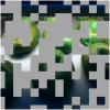
AttMask-High
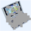
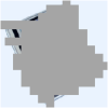
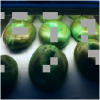
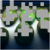
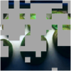
AttMask-Hint
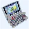
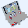
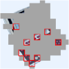
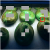
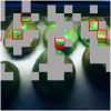
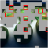
Block-Wise
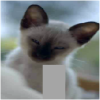
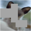
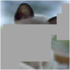
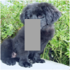
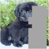
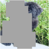
Random
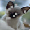
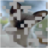
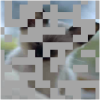
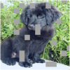
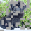
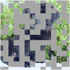
AttMask-High
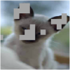
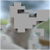
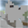
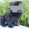
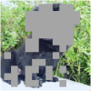
AttMask-Hint

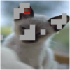
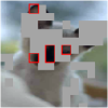
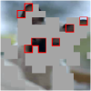
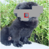
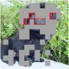
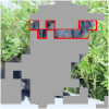
Figure A6: Illustration of different masking strategies vs. mask ratio $r$ (%) (part 1). We compare random Block-Wise masking (BEiT [2]) with Random masking (SimMIM [72]), AttMask-High and AttMask-Hint. Our AttMask-High uses the attention map arising in the encoder to hide patches, while AttMask-Hint reveals very salient patches to leave hints about the identity of the masked object.

	10%	30%	50%			10%	30%	50%
Block-Wise
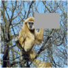
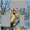
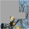
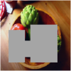
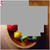
Random
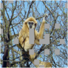
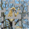
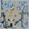
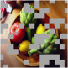
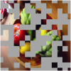
AttMask-High
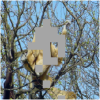
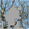
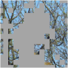
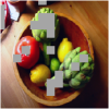
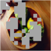
AttMask-Hint
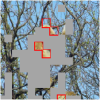
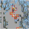
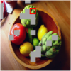
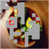
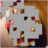
Block-Wise
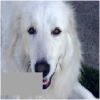
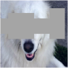
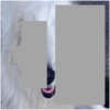
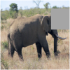
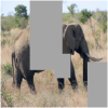
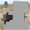
Random
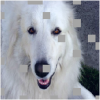
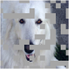
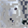
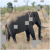
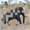
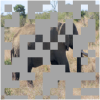
AttMask-High
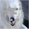
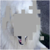
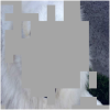
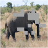
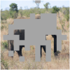
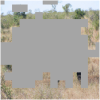
AttMask-Hint

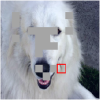
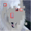
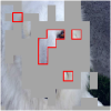
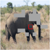
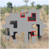
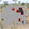
Figure A7: Illustration of different masking strategies vs. mask ratio $r$ (%) (part 2). We compare random Block-Wise masking (BEiT [2]) with Random masking (SimMIM [72]), AttMask-High and AttMask-Hint. Our AttMask-High uses the attention map arising in the encoder to hide patches, while AttMask-Hint reveals very salient patches to leave hints about the identity of the masked object.

Visualization of Masking Examples.

We illustrate the effect of mask ratio $r$ (%) to various masking strategies in Figure A6 and Figure A7. While random Block-Wise and Random masking fail to consistently mask informative parts of an image, AttMask-High and AttMask-Hint make use of attention to hide salient and all but very salient parts respectively. This gives rise to a more challenging MIM task.

Appendix 0.B Experimental Setup

We provide more details on the experimental setup, including multi-crop, training details and evaluation details.

Multi-Crop.

Following [8, 78], we apply the multi-crop strategy [7] to generate a set of $m$ low-resolution local crops, which cover only small parts of the image, tokenized as $Z^{c}_{1},\dots,Z^{c}_{m}$. Similar to $L_{\textsc{g}}$ (4), the loss is applied globally on the [cls] tokens, in particular between the student output for a local crop $Z^{c}_{j}$ and the teacher output for a global view $Z^{v}$, both of which are non-masked:

$$L_{\textsc{lc}}=-\sum_{v\in V}\sum_{j=1}^{m}f_{\theta^{\prime}}(Z^{v})^{\textsc{[cls]}}\log(f_{\theta}(Z^{c}_{j})^{\textsc{[cls]}}).$$ (A13)

The overall loss is a weighted sum of $L_{\textsc{mim}}$ (3), $L_{\textsc{g}}$ (4) and $L_{\textsc{lc}}$ (A13).

Training Details.

For our analysis and ablation (subsection 4.2, subsection 4.4 and subsection 0.A.2), we pre-train models on 20% of ImageNet-1k for 100 epochs. For both iBOT and DINO we use AdamW [42] as optimizer. Unless otherwise stated, we use the ViT-S/16 architecture and a batch size of 240. We warm-up learning rate $\eta$ for 10 epochs following the linear scaling rule $\eta=5\times 10^{-4}\times\texttt{bs}/256$ where bs is the batch size and then decay using a cosine schedule. We also use a cosine schedule from $0.04$ to $0.4$ for weight decay. We set teacher momentum to $0.99$ and student temperature to $0.1$. We use a linear warm-up for teacher temperature from $0.04$ to $0.07$ for the first 30 epochs following DINO.

All methods in subsection 4.2, subsection 4.4 and subsection 0.A.2 use the multi-crop scheme with two $224^{2}$ global crops and six $96^{2}$ local crops that approximately scale the training time by a factor of $\gamma=2+6\times(96/224)^{2}=3.10$. We use color jittering, Gaussian blur and solarization as data augmentations. Local crops scales are sampled from $(0.05,s)$ and global crop scales from $(s,1)$. We set $s$ to $0.4$ for DINO and $0.25$ for iBOT. We set the dimensionality of the head output to $65536$ for DINO, while for iBOT, we use a shared projection head for [CLS] and patch tokens, of dimensionality $8192$. We do not perform weight normalization on the last layer of the MLP heads.

For our benchmark (subsection 4.3 and subsection 0.A.1), we pre-train models on 100% of ImageNet-1k for 100 and 300 epochs. For the 100-epoch experiments, the setup is the same as on 20% of ImageNet-1k except for increasing the teacher momentum to $0.996$ and the number of local crops to ten. The scaling factor of the training time in this case is $\gamma=2+10\times(96/224)^{2}=3.84$. For the 300 epochs experiments, we increase the batch size to 800 and set $s$ to $0.32$, similar to the iBOT default scale.

Evaluation Details.

For the ImageNet-1k evaluation, we use $k$-NN and linear probing as in DINO [8] and iBOT [78]. We evaluate on ImageNet-1k validation set. For $k$-NN, we use the [CLS] feature from the last ViT layer and set $k$ to 20. For linear probing, we train a linear classifier using SGD with a batch size of 1024 for 100 epochs. We set learning rate to $0.003$ and do not apply weight decay. We apply random resized crops and horizontal flips as data augmentations and keep the central crop. Following DINO [8] and iBOT [78], we use the concatenation of the [CLS] features from the last four layers as input to the linear classifier.

For the evaluation of downstream tasks with finetuning, we train models on CIFAR10, CIFAR100 [34] for 500 epochs and on Oxford Flowers [47] for 1000 epochs. We set learning rate to $7.5\times 10^{-6}$, weight decay to $0.05$ and use a batch size of 900.

On COCO [39], we evaluate the performance of object detection and instance segmentation downstream tasks. We consider the COCO 2017 set, which contains $118$K training images, $5$k validation and $20$ test-dev. We consider the Cascade Mask R-CNN [4, 25] as task layer and follow the setup from [40]. We use the hyper-parameter configuration from [78]: multi-scale training (resizing image with shorter size between $480$ and $800$, with the longer side no larger than $1333$). We use AdamW [42] with initial learning rate $10^{-4}$, the $1\times$ schedule (12 epochs with the learning rate decayed by $10\times$ at epochs $9$ and $11$) and weight decay $0.05$. Unlike [78], where training is on $8$ GPUs with $4$ images per GPU, we use $2$ images per GPU due to hardware limitations. For a fair and direct comparison, we fine-tune iBOT baseline with the same configuration.

We evaluate on ADE20K [77] for the semantic segmentation downstream task. It consists of 25k images in 150 classes, with 20k for training, 2k for validation and 3k for testing. We rely on UperNet [70] as task layer and fine-tune the entire network following the setup from [40]: $160$k iterations with $512\times 512$ images. We do not perform multi-scale training and testing. We adopt the same hyper-parameters as in [78]. We use the AdamW [42] optimizer with an initial learning rate of $7\times 10^{-4}$ with poly-scheduling, layer decay rate $0.65$ and weight decay $0.05$. We train on $8$ GPUs with $2$ images per GPU.

For the evaluation of downstream tasks without finetuning, we follow the protocol of DINO on $\mathcal{R}$Oxford, $\mathcal{R}$Paris [53] and DAVIS 2017 [52]. On Caltech-UCSD Birds (CUB200) [64], Cars (CARS196) [33], Stanford Online Products (SOP) [49] and In-Shop Clothing Retrieval (In-Shop) [41], we extract features from test set images and directly apply nearest neighbor search to measure Recall@$k$ [49]. On Places205 [76], we train a $205$-way linear classifier on pre-cached features, using only horizontal flip as augmentation. Training is with SGD for $50$ epochs using an initial learning rate of $0.01$ that is decreased to $0$ with cosine schedule, a batch-size of $1024$, and no weight decay.

References

- [1] Arandjelovic, R., Zisserman, A.: Look, listen and learn. In: Proceedings of the IEEE International Conference on Computer Vision. pp. 609–617 (2017)
- [2] Bao, H., Dong, L., Piao, S., Wei, F.: BEit: BERT pre-training of image transformers. In: International Conference on Learning Representations (2022)
- [3] Cai, T.T., Frankle, J., Schwab, D.J., Morcos, A.S.: Are all negatives created equal in contrastive instance discrimination? arXiv preprint arXiv:2010.06682 (2020)
- [4] Cai, Z., Vasconcelos, N.: Cascade r-cnn: high quality object detection and instance segmentation. IEEE transactions on pattern analysis and machine intelligence (2019)
- [5] Caron, M., Bojanowski, P., Joulin, A., Douze, M.: Deep clustering for unsupervised learning of visual features. In: Proceedings of the European Conference on Computer Vision. pp. 132–149 (2018)
- [6] Caron, M., Bojanowski, P., Mairal, J., Joulin, A.: Unsupervised pre-training of image features on non-curated data. In: Proceedings of the IEEE/CVF International Conference on Computer Vision. pp. 2959–2968 (2019)
- [7] Caron, M., Misra, I., Mairal, J., Goyal, P., Bojanowski, P., Joulin, A.: Unsupervised learning of visual features by contrasting cluster assignments. Advances in Neural Information Processing Systems 33, 9912–9924 (2020)
- [8] Caron, M., Touvron, H., Misra, I., Jégou, H., Mairal, J., Bojanowski, P., Joulin, A.: Emerging properties in self-supervised vision transformers. In: Proceedings of the IEEE/CVF International Conference on Computer Vision. pp. 9650–9660 (2021)
- [9] Chen, T., Kornblith, S., Norouzi, M., Hinton, G.: A simple framework for contrastive learning of visual representations. In: International Conference on Machine Learning. pp. 1597–1607. PMLR (2020)
- [10] Chen, X., He, K.: Exploring simple siamese representation learning. In: Proceedings of the IEEE/CVF Conference on Computer Vision and Pattern Recognition. pp. 15750–15758 (2021)
- [11] Child, R., Gray, S., Radford, A., Sutskever, I.: Generating long sequences with sparse transformers. arXiv preprint arXiv:1904.10509 (2019)
- [12] Choe, J., Shim, H.: Attention-based dropout layer for weakly supervised object localization. In: Proceedings of the IEEE/CVF Conference on Computer Vision and Pattern Recognition. pp. 2219–2228 (2019)
- [13] Cordonnier, J.B., Loukas, A., Jaggi, M.: On the relationship between self-attention and convolutional layers. In: International Conference on Learning Representations (2020)
- [14] Deng, J., Dong, W., Socher, R., Li, L.J., Li, K., Fei-Fei, L.: Imagenet: A large-scale hierarchical image database. In: IEEE Conference on Computer Vision and Pattern Recognition. pp. 248–255. Ieee (2009)
- [15] Devlin, J., Chang, M.W., Lee, K., Toutanova, K.: Bert: Pre-training of deep bidirectional transformers for language understanding. In: Proceedings of the 2019 Conference of the North American Chapter of the Association for Computational Linguistics: Human Language Technologies, Volume 1 (Long and Short Papers). pp. 4171–4186 (2019)
- [16] Doersch, C., Gupta, A., Efros, A.A.: Unsupervised visual representation learning by context prediction. In: Proceedings of the IEEE International Conference on Computer Vision. pp. 1422–1430 (2015)
- [17] Dosovitskiy, A., Beyer, L., Kolesnikov, A., Weissenborn, D., Zhai, X., Unterthiner, T., Dehghani, M., Minderer, M., Heigold, G., Gelly, S., et al.: An image is worth 16x16 words: Transformers for image recognition at scale. In: International Conference on Learning Representations (2020)
- [18] Falcon, W., Cho, K.: A framework for contrastive self-supervised learning and designing a new approach. arXiv preprint arXiv:2009.00104 (2020)
- [19] Ghiasi, G., Lin, T.Y., Le, Q.V.: Dropblock: A regularization method for convolutional networks. Advances in Neural Information Processing Systems 31 (2018)
- [20] Gidaris, S., Bursuc, A., Komodakis, N., Pérez, P., Cord, M.: Learning representations by predicting bags of visual words. In: Proceedings of the IEEE Conference on Computer Vision and Pattern Recognition (2020)
- [21] Gidaris, S., Bursuc, A., Puy, G., Komodakis, N., Cord, M., Pérez, P.: Obow: Online bag-of-visual-words generation for self-supervised learning. In: Proceedings of the IEEE Conference on Computer Vision and Pattern Recognition (2021)
- [22] Gidaris, S., Singh, P., Komodakis, N.: Unsupervised representation learning by predicting image rotations. In: International Conference on Learning Representations (2018)
- [23] Grill, J.B., Strub, F., Altché, F., Tallec, C., Richemond, P., Buchatskaya, E., Doersch, C., Avila Pires, B., Guo, Z., Gheshlaghi Azar, M., et al.: Bootstrap your own latent-a new approach to self-supervised learning. Advances in Neural Information Processing Systems 33, 21271–21284 (2020)
- [24] He, K., Chen, X., Xie, S., Li, Y., Dollár, P., Girshick, R.: Masked autoencoders are scalable vision learners. In: Proceedings of the IEEE/CVF Conference on Computer Vision and Pattern Recognition (CVPR). pp. 16000–16009 (2022)
- [25] He, K., Gkioxari, G., Dollár, P., Girshick, R.: Mask r-cnn. In: Proceedings of the IEEE international conference on computer vision (2017)
- [26] He, K., Zhang, X., Ren, S., Sun, J.: Deep residual learning for image recognition. In: Proceedings of the IEEE Conference on Computer Vision and Pattern Recognition. pp. 770–778 (2016)
- [27] Ho, J., Kalchbrenner, N., Weissenborn, D., Salimans, T.: Axial attention in multidimensional transformers. arXiv preprint arXiv:1912.12180 (2019)
- [28] Hou, Q., Jiang, P., Wei, Y., Cheng, M.M.: Self-erasing network for integral object attention. In: Advances in Neural Information Processing Systems (2018)
- [29] Ioffe, S., Szegedy, C.: Batch normalization: Accelerating deep network training by reducing internal covariate shift. In: International Conference on Machine Learning. pp. 448–456. PMLR (2015)
- [30] Kalantidis, Y., Sariyildiz, M.B., Pion, N., Weinzaepfel, P., Larlus, D.: Hard negative mixing for contrastive learning. Advances in Neural Information Processing Systems 33, 21798–21809 (2020)
- [31] Kim, D., Cho, D., Yoo, D., So Kweon, I.: Two-phase learning for weakly supervised object localization. In: Proceedings of the IEEE/CVF International Conference on Computer Vision (2017)
- [32] Kolesnikov, A., Zhai, X., Beyer, L.: Revisiting self-supervised visual representation learning. In: Proceedings of the IEEE/CVF Conference on Computer Vision and Pattern Recognition. pp. 1920–1929 (2019)
- [33] Krause, J., Stark, M., Deng, J., Li, F.F.: 3d object representations for fine-grained categorization. ICCVW (2013)
- [34] Krizhevsky, A., Hinton, G., et al.: Learning multiple layers of features from tiny images (2009)
- [35] Krizhevsky, A., Sutskever, I., Hinton, G.E.: Imagenet classification with deep convolutional neural networks. In: Proceedings of the 25th International Conference on Neural Information Processing Systems - Volume 1. p. 1097–1105. NIPS’12, Curran Associates Inc., Red Hook, NY, USA (2012)
- [36] Lee, H.Y., Huang, J.B., Singh, M., Yang, M.H.: Unsupervised representation learning by sorting sequences. In: Proceedings of the IEEE International Conference on Computer Vision. pp. 667–676 (2017)
- [37] Li, J., Zhou, P., Xiong, C., Hoi, S.: Prototypical contrastive learning of unsupervised representations. In: International Conference on Learning Representations (2021)
- [38] Li, Z., Chen, Z., Yang, F., Li, W., Zhu, Y., Zhao, C., Deng, R., Wu, L., Zhao, R., Tang, M., et al.: Mst: Masked self-supervised transformer for visual representation. Advances in Neural Information Processing Systems 34 (2021)
- [39] Lin, T.Y., Maire, M., Belongie, S., Hays, J., Perona, P., Ramanan, D., Dollár, P., Zitnick, C.L.: Microsoft coco: Common objects in context. In: European Conference on Computer Vision. pp. 740–755. Springer (2014)
- [40] Liu, Z., Lin, Y., Cao, Y., Hu, H., Wei, Y., Zhang, Z., Lin, S., Guo, B.: Swin transformer: Hierarchical vision transformer using shifted windows. In: Proceedings of the IEEE/CVF International Conference on Computer Vision (2021)
- [41] Liu, Z., Luo, P., Qiu, S., Wang, X., Tang, X.: Deepfashion: Powering robust clothes recognition and retrieval with rich annotations. In: Proceedings of the IEEE Conference on Computer Vision and Pattern Recognition (2016)
- [42] Loshchilov, I., Hutter, F.: Decoupled weight decay regularization. In: International Conference on Learning Representations (2018)
- [43] Misra, I., Maaten, L.v.d.: Self-supervised learning of pretext-invariant representations. In: Proceedings of the IEEE/CVF Conference on Computer Vision and Pattern Recognition. pp. 6707–6717 (2020)
- [44] Misra, I., Zitnick, C.L., Hebert, M.: Shuffle and learn: unsupervised learning using temporal order verification. In: European Conference on Computer Vision. pp. 527–544. Springer (2016)
- [45] Musgrave, K., Belongie, S., Lim, S.N.: A metric learning reality check. In: European Conference on Computer Vision (2020)
- [46] Nilsback, M.E., Zisserman, A.: Automated flower classification over a large number of classes. In: Proceedings of the Indian Conference on Computer Vision, Graphics and Image Processing (Dec 2008)
- [47] Nilsback, M.E., Zisserman, A.: Automated flower classification over a large number of classes. In: Indian Conference on Computer Vision, Graphics and Image Processing (Dec 2008)
- [48] Noroozi, M., Favaro, P.: Unsupervised learning of visual representations by solving jigsaw puzzles. In: European conference on Computer Vision. pp. 69–84. Springer (2016)
- [49] Oh Song, H., Xiang, Y., Jegelka, S., Savarese, S.: Deep metric learning via lifted structured feature embedding. In: Proceedings of the IEEE Conference on Computer Vision and Pattern Recognition (2016)
- [50] Van den Oord, A., Li, Y., Vinyals, O.: Representation learning with contrastive predictive coding. arXiv e-prints pp. arXiv–1807 (2018)
- [51] Parmar, N., Vaswani, A., Uszkoreit, J., Kaiser, L., Shazeer, N., Ku, A., Tran, D.: Image transformer. In: International Conference on Machine Learning. pp. 4055–4064. PMLR (2018)
- [52] Perazzi, F., Pont-Tuset, J., McWilliams, B., Van Gool, L., Gross, M., Sorkine-Hornung, A.: A benchmark dataset and evaluation methodology for video object segmentation. In: Proceedings of the IEEE Conference on Computer Vision and Pattern Recognition (2016)
- [53] Radenović, F., Iscen, A., Tolias, G., Avrithis, Y., Chum, O.: Revisiting oxford and paris: Large-scale image retrieval benchmarking. In: Proceedings of the IEEE Conference on Computer Vision and Pattern Recognition. pp. 5706–5715 (2018)
- [54] Radosavovic, I., Kosaraju, R.P., Girshick, R., He, K., Dollar, P.: Designing network design spaces. In: Proceedings of the IEEE/CVF Conference on Computer Vision and Pattern Recognition (2020)
- [55] Simonyan, K., Zisserman, A.: Very deep convolutional networks for large-scale image recognition. In: Bengio, Y., LeCun, Y. (eds.) International Conference on Learning Representations (2015)
- [56] Srivastava, N., Hinton, G., Krizhevsky, A., Sutskever, I., Salakhutdinov, R.: Dropout: A simple way to prevent neural networks from overfitting. Journal of Machine Learning Research 15(56), 1929–1958 (2014)
- [57] Stojnic, V., Risojevic, V.: Self-supervised learning of remote sensing scene representations using contrastive multiview coding. In: Proceedings of the IEEE/CVF Conference on Computer Vision and Pattern Recognition. pp. 1182–1191 (2021)
- [58] Sun, C., Shrivastava, A., Singh, S., Gupta, A.: Revisiting unreasonable effectiveness of data in deep learning era. In: Proceedings of the IEEE International Conference on Computer Vision. pp. 843–852 (2017)
- [59] Szegedy, C., Liu, W., Jia, Y., Sermanet, P., Reed, S., Anguelov, D., Erhan, D., Vanhoucke, V., Rabinovich, A.: Going deeper with convolutions. In: Proceedings of the IEEE Conference on Computer Vision and Pattern Recognition. pp. 1–9 (2015)
- [60] Tarvainen, A., Valpola, H.: Mean teachers are better role models: Weight-averaged consistency targets improve semi-supervised deep learning results (2017)
- [61] Tompson, J., Goroshin, R., Jain, A., LeCun, Y., Bregler, C.: Efficient object localization using convolutional networks. In: Proceedings of the IEEE Conference on Computer Vision and Pattern Recognition. pp. 648–656 (2015)
- [62] Touvron, H., Cord, M., Douze, M., Massa, F., Sablayrolles, A., Jégou, H.: Training data-efficient image transformers & distillation through attention. In: International Conference on Machine Learning. pp. 10347–10357. PMLR (2021)
- [63] Vaswani, A., Shazeer, N., Parmar, N., Uszkoreit, J., Jones, L., Gomez, A.N., Kaiser, Ł., Polosukhin, I.: Attention is all you need. Advances in Neural Information Processing Systems 30 (2017)
- [64] Wah, C., Branson, S., Welinder, P., Perona, P., Belongie, S.: The Caltech-UCSD Birds-200-2011 Dataset. Tech. Rep. CNS-TR-2011-001, California Institute of Technology (2011)
- [65] Wang, H., Zhu, Y., Green, B., Adam, H., Yuille, A., Chen, L.C.: Axial-deeplab: Stand-alone axial-attention for panoptic segmentation. In: European Conference on Computer Vision. pp. 108–126. Springer (2020)
- [66] Wang, T., Isola, P.: Understanding contrastive representation learning through alignment and uniformity on the hypersphere. In: International Conference on Machine Learning. pp. 9929–9939. PMLR (2020)
- [67] Weissenborn, D., Täckström, O., Uszkoreit, J.: Scaling autoregressive video models. In: International Conference on Learning Representations (2020)
- [68] Wu, Z., Xiong, Y., Yu, S.X., Lin, D.: Unsupervised feature learning via non-parametric instance discrimination. In: Proceedings of the IEEE Conference on Computer Vision and Pattern Recognition. pp. 3733–3742 (2018)
- [69] Xiao, K., Engstrom, L., Ilyas, A., Madry, A.: Noise or signal: The role of image backgrounds in object recognition. In: International Conference on Learning Representations (2021)
- [70] Xiao, T., Liu, Y., Zhou, B., Jiang, Y., Sun, J.: Unified perceptual parsing for scene understanding. In: Proceedings of the European Conference on Computer Vision (ECCV) (2018)
- [71] Xie, Z., Lin, Y., Yao, Z., Zhang, Z., Dai, Q., Cao, Y., Hu, H.: Self-supervised learning with swin transformers. arXiv preprint arXiv:2105.04553 (2021)
- [72] Xie, Z., Zhang, Z., Cao, Y., Lin, Y., Bao, J., Yao, Z., Dai, Q., Hu, H.: Simmim: A simple framework for masked image modeling. In: Proceedings of the IEEE/CVF Conference on Computer Vision and Pattern Recognition (CVPR). pp. 9653–9663 (2022)
- [73] YM., A., C., R., A., V.: Self-labelling via simultaneous clustering and representation learning. In: International Conference on Learning Representations (2020)
- [74] Zhang, L., Qi, G.J., Wang, L., Luo, J.: Aet vs. aed: Unsupervised representation learning by auto-encoding transformations rather than data. In: Proceedings of the IEEE/CVF Conference on Computer Vision and Pattern Recognition. pp. 2547–2555 (2019)
- [75] Zhang, X., Wei, Y., Feng, J., Yang, Y., Huang, T.S.: Adversarial complementary learning for weakly supervised object localization. In: Proceedings of the IEEE Conference on Computer Vision and Pattern Recognition (June 2018)
- [76] Zhou, B., Lapedriza, A., Xiao, J., Torralba, A., Oliva, A.: Learning deep features for scene recognition using places database. In: Advances in Neural Information Processing Systems (2014)
- [77] Zhou, B., Zhao, H., Puig, X., Fidler, S., Barriuso, A., Torralba, A.: Scene parsing through ade20k dataset. In: Proceedings of the IEEE Conference on Computer Vision and Pattern Recognition. pp. 633–641 (2017)
- [78] Zhou, J., Wei, C., Wang, H., Shen, W., Xie, C., Yuille, A., Kong, T.: ibot: Image bert pre-training with online tokenizer. In: International Conference on Learning Representations (2022)
- [79] Zhuang, C., Zhai, A.L., Yamins, D.: Local aggregation for unsupervised learning of visual embeddings. In: Proceedings of the IEEE/CVF International Conference on Computer Vision. pp. 6002–6012 (2019)