1%\vspace{-0.2in}
2\end{figure}
3
4Having described the landscape of object replication (deep vs. shallow, some time window vs. full lifespan, mutable vs. immutable, and memory size vs. access counts), we now scope this problem to a tractable subset driven by pragmatic tool-development factors.
5First, instrumenting every allocation and memory access to identify object replicas leads to excessive runtime overheads; we seek for a lightweight tool that can collect profiles in production rather than in test-only environments; we guarantee the analysis accuracy with the theoretical bounds of a sampling technique we use.
6Second, deep replica comparison is unachievable without running something analogous to the garbage collector, which can introduce high overheads and require runtime modifications, making it less adaptable; hence we restrict our tool to only shallow object comparison.
7Third, if two objects are not replicas for their entire life span, they are not easy to optimize, and hence we consider only those objects that are replicas for their entire duration.
8We do not enforce objects to be immutable for replica detection.
9Finally, our tool regards two or more objects as replicas only if they were allocated in the same calling context; the observation drives this restriction that it is significantly easy to refactor such code to optimize compared with optimizing replica objects allocated from myriad code locations.
10We emphasize that we want to be able to monitor replicas and prioritize them by their access frequency.
11
12\begin{comment}
13Software inefficiencies are everywhere in computer systems ranging from smartphones to supercomputers and data centers.
14Software packages have become increasingly complex at the code level, comprised of a large amount of source code, multi-layer abstractions, and deep call chains. Without careful design and monitoring, software developers can easily introduce performance inefficiencies embedded deep in the code bases that go unnoticed or remain challenging to diagnose, leading to performance degradation.
15Hardware evolution outpaces the performance optimization of software at the resource level, leading to resource wastage and energy dissipation in emerging architectures.
16Even worse, due to JVM, a step removed from the underlying hardware makes JVM-based managed languages suffer from worse performance than native languages.
17
18Performance profiling tools abound in the Java community to aid software developers in understanding program behavior. Profiling for execution hotspots and inefficiencies are the most popular ones.
19Hotspot analysis profilers~\cite{netbeans-WWW,jprofiler-WWW,yourkit-WWW,visualvm-WWW,oracle-studio-WWW,perf,async-profiler-WWW,Levon:OProfile} identify code regions that consume a large portion of resources disregarding whether these resources are being used productively; instead, tool users need to make a judgment call.
20Inefficiency analysis profilers~\cite{Cachetor,Memoization,toddler,ldoctor,Flow,Containers,Reusable,pmu-java-behavior,Vertical,inefficiencies-in-java,remix} identify code regions that waste resources instead of consuming resources.
21Distinguished from hotspot analysis tools, inefficiency analysis can guide users to concentrate on code regions involved in some inefficiency.
22
23
24
25A Java object is a combination of properties and methods working on the properties. Software developers primarily think of Java code in terms of objects which form mental boundaries of functionality. It is natural that when developers investigate performance inefficiencies, they often tend to analyze the code at the object-level granularity.
26A recent line of inefficiency analysis tools have demonstrated that redundancies are a significant software inefficiency indicator in both native languages~\cite{Chabbi:2012:DTP:2259016.2259033,Wen:2017:REV:3037697.3037729,Su:2019:RLS:3339505.3339628,witch} and managed languages~\cite{inefficiencies-in-java,toddler,ldoctor,Dhok:2016:DTG:2950290.2950360,DellaToffola:2015:PPY:2814270.2814290} such as Java. However, they are missing a critical piece --- object duplications that happen across objects sharing the same calling context.
27Based on many case studies in this paper, our observation is that various kinds of inefficiencies are due to object duplications.
28
29To overcome this critical missing piece, we propose \tool{}, a \emph{lightweight} sampling-based performance analysis profiler for pinpointing object duplications by tracking the contents of different objects that share the same allocation context.
30\tool{} complements existing Java profilers by employing PMUs to sample memory locations accessed by an object and employing debug registers to monitor memory locations accessed by the objects that are subsequently allocated at the same context.
31
32\end{comment}
33
34
35\tool{}, developed to meet these factors, monitors object allocations and accesses at runtime via statistical sampling.
36%Keeping track of each object allocation can incur a high overhead. Hence, \tool{} uses a configurable parameter $\mathcal{S}$ to only monitor objects of the size larger than $\mathcal{S}$ to trade off the overhead.
37%In our experiments, we set $\mathcal{S}$ to 1KB because we do not find any interesting optimizations on small objects.
38The key differentiating aspect of \tool{}, compared to a large class of existing profilers, is its ability to detect object replicas with minimal byte code instrumentation and no prior knowledge of programs makes it applicable in the production environment.
39A thorough evaluation of several real-world applications shows that pinpointing object replicas offers new avenues to understanding performance losses; aggregating replica objects into one or a few objects reduces the memory footprint, eliminates redundant computations, and enhances performance.
40
41%In the rest of this section, we show a motivating example, summarize the contributions of this paper, and overview the paper organization.
42
43
44\subsection{Observation}
45
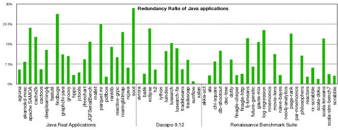
46With the help of \tool{}, Figure~\ref{redundancy ratio} quantifies the ratio of object replicas over the total number of objects in several real applications listed at~\cite{awesome-java} and two popular Java benchmark suites---Dacapo 9.12~\cite{dacapo-9.12} and Renaissance~\cite{Prokopec:2019:RBS:3314221.3314637}, showing that replicated objects are pervasive in modern Java software packages.
47Based on many case studies investigated in this paper, we observe that object replication is the symptom of the following kinds of inefficiencies.
48
49\paragraph{\textbf{\textit{Input-sensitive Inefficiencies.}}}
50%Repeatedly passing same parameters to a Java constructor shows up as repeatedly creating objects with the same content.
51Repeatedly using the same input to instantiate a Java class shows up as repeatedly creating objects with the same content.
52Listing~\ref{motivation parquet} shows a problematic method \texttt{readNext} from Parquet-MR~\cite{parquet-mr}, which contains the Java implementation of the Parquet format.
53This method is invoked in a loop, and in each invocation, it creates a new object \texttt{bytes}, shown on line 93, and initializes this object via input stream ‘‘in’’, as shown on line 94.
54We run Parquet-MR using Parquet-Column as its input.
55The Parquet-Column input is a columnar storage format for Hadoop; this format provides efficient storage and encoding of data. As line 94 in Listing 1 shows, each time the readNext method is invoked, it creates a copy of input contents (variable “in”), and uses this copy to initialize many objects “bytes” (object replication).
56None of the existing profilers, such as JXPerf~\cite{inefficiencies-in-java} and LDoctor~\cite{ldoctor}, can identify such object replicas since they are designed only to recognize the redundancies happening at the same memory location.
57Instead, objects \texttt{bytes} are allocated in disjoint memory regions.
58
59\paragraph{\textbf{\textit{Algorithmic Inefficiencies.}}}
60Suboptimal choices of an algorithm often show up as object duplications.
61As a practical example, Findbugs~\cite{FindBugs} divides a graph into tiny-size blocks and creates an object for each block instead of creating a single object for the whole graph. Consequently, most of the created objects have the same content due to good value locality among adjacent blocks.
62
63\paragraph{\textbf{\textit{Data Structural Inefficiencies.}}}
64Like suboptimal algorithms, poor data structures can easily introduce object replicas as well. For instance, in matrix multiplication, sparse matrices with a dense format can yield a high proportion of objects with the same content.\\
65
66The major lessons that can be learned from this paper:
67\begin{itemize}[leftmargin=*]
68\item Object replicas are not uncommon in real Java applications.
69\item Sampling-based measurement based on hardware counters and debug registers can provide good insights and incur significant low overhead.
70\item Developing OJXPerf that efficiently interacts with off-the-shelf JVM and Linux OS in the production environment requires careful design.
71\item The call path of object allocation and source code attribution in a GUI are particularly useful for users to identify actionable optimization.
72\end{itemize}
73
74%The above categories suffice to offer an intuition about the class of inefficiencies detectable by observing object replicas.
75
76
77
78\begin{comment}
79The object that suffers from object-level redundancy, array bytes, is at on line 96 in method readNext of class RunLengthBitPackingHybridDecoder, shown in listing~\ref{motivation parquet}. The program creates the array bytes (line 93) in every invocation of method readNext. After each creation of array bytes, the program uses DataInputStream to read the input stream into the array bytes. Then, the program calls the method \texttt{unpack8Values} to unpack the data contained in bytes to the output array currentBuffer. \tool{} reports that the array bytes has 90.0\% chance of equal with the array bytes from the last invocation of this method. In this example, we can see that these array bytes allocated in every invocation of method \texttt{readNext} are separate objects and they are allocated into different memory locations. Previous proposed works only can detect redundancy like, if method \texttt{readNext} creates one array byte, and this array byte is accessed for several times inside one invocation of method \texttt{readNext}. Thus, previous proposed works only monitor the same memory location, instead of the different memory locations shown in above motivation example.
80
81Some Java applications have design issues, which lead to the object-level redundancy. For example, the Java application Apache SAMOA. The problematic object that suffers from object-level redundancy issue happen in method copyObject of class SerializeUtils. With further investigation, we find that the program processes a sequent of events. Before processing each event, the program performs an object copy operation. However, we find that many processes are designed to copy an object that will not be changed for a period of time, which result to the copy procedure generates some objects that have the same content (object-level redundancy). In this case, the program can be redesigned as the copy procedure is performed only once if the object is not changed, then each process can use the copy result directly instead of copy the object again.
82
83For some other Java applications, which use graph or map as input, always suffer from object-level redundancy. The reason is that instead of putting the whole graph or map as one time input, these Java applications usually divide a big graph or map into a number of small blocks. And then these small blocks will be used as input for execution. For example, the Java application Findbugs, which has the problematic objects that suffer from object level redundancy issue happen in method \texttt{getStartFact} and method \texttt{getResultFact} of class BasicAbstractDataflowAnalysis. After checking the call path, we find that the program runs its algorithm and divides a whole CFG into many blocks as input in execute method of Dataflow class. In some cases, we find that some adjacent blocks of CFG are identical. Based on these identical small blocks as input, Findbugs usually have some redundancy computations, which lead to the object-level redundancy.
84
85Also, some Java applications initialize some data in their constructor methods before do some computations. For example, the Java application Soot. The problematic objects that suffer from object-level redundancy issue happen in method orAndAndNot of class BitVector. With further investigation, we find that the program has some redundant computations and creates the same content objects repeatedly. The reason is that some computations are based on an array bits which is initialized in constructor. Because usually the program will not call the constructor very frequently, which means that the initialized array bits will keep same for a period of time. In such period of time, the computations will generate some objects that have identical contents.
86\end{comment}
87
88
89
90
91\subsection{Paper Contributions}
92In this paper, \tool{} makes the following contributions:
93\begin{itemize}[leftmargin=*]
94\item Develops a novel object-centric profiling technique. It provides rich information to guide optimizing object replicas in JVM-based programs, such as Java and Scala.
95\item Employs PMU in conjunction with hardware debug registers and minimal byte code instrumentation, which typically incurs 9\% runtime and 6\% memory overheads.
96\item Quantifies the theoretical lower and upper bounds of replication ratios of \tool{}’s statistical approach.
97\item Applies to unmodified Java (and languages based on JVM, e.g., Scala) applications, the off-the-shelf Java virtual machine, and Linux operating system, running on commodity CPU processors, which can be directly deployed in the production environment.
98\sloppy
99\item Provides intuitive optimization guidance for developers. We evaluate \tool{} with popular Java benchmarks (Dacapo~\cite{dacapo}, NPB~\cite{npb}, Grande~\cite{grande}, SPECjvm2008~\cite{specjvm2008}, and the most recent Renaissance~\cite{Prokopec:2019:RBS:3314221.3314637}) and more than 20 real-world applications. Guided by \tool{}, we are able to obtain significant speedups by eliminating object replicas in various Java programs. We have upstreamed some of the patches to the software repositories.
100\end{itemize}
101
102\subsection{Paper Organization}
103The paper is organized as follows. Section~\ref{relate} covers the related work and distinguishes \tool{}. Section~\ref{background} offers some background knowledge. Section~\ref{methodology} depicts \tool{}’s methodology. Section~\ref{implementation} describes the implementation details of \tool{}. Section~\ref{theory} discusses the theoretical guarantee of \tool{}’s analysis accuracy. Section~\ref{evaluation} evaluates \tool{}’s accuracy and overhead. Section~\ref{case study} describes case studies of \tool{}. Section~\ref{validity} discusses the threats to validity. Finally, Section~\ref{conclusion} presents our conclusions.
104
105
106
107\section{Related Work}
108\label{relate}
109Performance profiling techniques abound in the Java community, which fall into two categories: hardware and software approaches. Each category can be further classified into hotspot and inefficiency analyses. We also compare the related Java tools in table~\ref{comparison}.
110
111\begin{table}
112\centering
113\includegraphics[width=0.49\textwidth]{images/comparison.pdf}
114\caption{Comparing OJXPerf with other state-of-the-art inefficiency analysis tools/approaches.}
115\label{comparison}
116\vspace{-1em}
117\end{table}
118
119\subsection{Software Approaches}
120\paragraph{\textbf{\textit{Hotspot Analysis.}}}
121\sloppy
122Netbeans Profiler~\cite{netbeans-WWW}, JProfiler~\cite{jprofiler-WWW}, YourKit~\cite{yourkit-WWW}, VisualVM~\cite{visualvm-WWW}, and Oracle Developer Studio Performance Analyzer~\cite{oracle-studio-WWW} are hotspot analysis profilers, which identify execution hotspots in CPU time or memory usage. They typically introduce negligible overhead by leveraging OS timers as the sampling engines to deliver periodic samples.
123The hotspot analysis is indispensable but fails to tell whether a resource is being used in a productive manner and contributes to a program’s overall efficiencies.
124A hotspot does not need to be an inefficient code region and vice versa.
125Hence, a heavy burden is on users to make a judgment on whether the reported hotspots are actionable.
126
127\paragraph{\textbf{\textit{Inefficiency Analysis.}}}
128Unlike hotspot analysis, inefficiency analysis tools identify code regions leading to resource wastage instead of resource usage.
129Cachetor~\cite{Cachetor} combines value profiling and dependence profiling to pinpoint operations that repeatedly generate an identical value.
130MemoizeIt~\cite{Memoization} identifies methods that repeatedly perform identical computation.
131JOLT~\cite{LJOLT} identifies and optimizes object churn in a virtual machine.
132Toddler~\cite{toddler} identifies redundant memory load operations in loop nests.
133The follow-up work~\cite{ldoctor} applies a static-dynamic analysis to reduce Toddler’s overhead. However, it identifies inefficiencies within a small number of suspicious loops instead of the entire program.
134Xu \textsl{et al.}~\cite{Flow} introduce copy profiling that optimizes data copies to remove the objects that carry copied values, and the method calls that allocate and populate these objects. Their follow-up work~\cite{Containers} develops practical static and dynamic analyses that identify inefficiently-used containers, such as overpopulated containers and underutilized containers. They also present a run-time technique~\cite{Reusable} to identify reusable data structures to avoid frequent object allocations. OEP~\cite{OEP} identifies mergeability among live objects, which requires the measurement of object reachability. In contrast, OJXPerf analyzes objects allocated in the same call path regardless of their liveness. OEP leverages bytecode instrumentation, which incurs orders of magnitude of overhead compared to OJXPerf.
135
136\tool{} is a profiler but applies a hardware approach to address a different inefficiency problem --- object replication.
137
138\subsection{Hardware Approaches}
139There are many hardware-assisted profilers. In this paper, we review only PMU- or debug register-assisted Java profilers.
140
141\paragraph{\textbf{\textit{Hotspot Analysis.}}}
142Linux Perf~\cite{perf}, Async-profiler~\cite{async-profiler-WWW}, and Oprofile~\cite{Levon:OProfile} employ PMU as the sampling engines to deliver periodic samples. PMU-based hotspot profilers offer slightly better intuition than the OS timer-based ones since they can classify hotspots according to various forms of performance metrics collected from PMU, such as instruction numbers, cache misses, bandwidth, and many others. However, they are not panaceas; users still have to distinguish inefficient hotspots from efficient ones manually.
143
144\paragraph{\textbf{\textit{Inefficiency Analysis.}}}
145Sweeney \textsl{et al.}~\cite{pmu-java-behavior} develop a system that provides a graphical interface to alleviate the difficulty in interpreting PMU results. Hauswirth \textsl{et al.}~\cite{Vertical} present vertical profiling that captures and correlates performance problems across multiple execution layers (application, VM, OS, and hardware). Georges \textsl{et al.}~\cite{Phase} study methods exhibit similar and dissimilar behaviors by measuring the execution time for each method invocation using PMU. Lau \textsl{et al.}~\cite{auditing} present a technique that allows a VM to determine whether an optimization improved or degraded by measuring CPU cycles. Remix~\cite{remix} employs PMU to identify inter-thread false sharing on the fly.
146JXPerf~\cite{inefficiencies-in-java} detects redundant memory operations by using PMU to sample memory locations accessed by a program and using debug registers to monitor subsequent accesses to the same location.
147
148Orthogonal to the aforementioned inefficiency analysis profilers, \tool{} addresses a different inefficiency problem with a different usage of PMU and debug registers. To the best of our knowledge, \tool{} is the first lightweight sampling-based profiler to pinpoint object replicas in Java.
149
150\begin{comment}
151\paragraph{\textbf{\textit{Debug Register-assisted Profilers.}}}
152DataCollider~\cite{Data-race} leverages debug registers to identify data races in Windows and Jiang \textsl{et al.}~\cite{DRDDR} extends it to support Linux.
153Liu \textsl{et al.}~\cite{Liu:2016:DFP:2884781.2884784, Liu:2019:CCO:3314872.3314881} employ debug registers to detect memory corruption bugs, e.g., buffer overflows, use after free, and memory leaks.
154DProf~\cite{DProf} combines PMU and debug registers to construct the data flow across runtime objects.
155Witch~\cite{witch} detect redundant memory operations in native languages by using PMU to sample memory locations accessed by a program and using debug registers to monitor subsequent accesses to the same memory.
156Su \textsl{et al.}~\cite{inefficiencies-in-java} extend Witch to detect redundant memory operations in managed languages.
157RDX~\cite{featherlight} combines PMU and debug registers to measure whole-program data reuse distances.
158\end{comment}
159
160
161\section{Background}
162\label{background}
163
164We introduce some essential facilities that \tool{} leverages based on Java virtual machines (JVM) and CPU processors.
165
166\begin{comment}
167\paragraph{\textbf{\textit{ASM Framework.}}}
168ASM~\cite{asm} is a Java byte code manipulation tool designed to generate and manipulate Java classes dynamically. ASM provides two APIs for generating and transforming compiled classes: the core API that provides an event-based representation of classes and the tree API that provides an object-based representation.
169% The two APIs manage only one class at a time, independently of each other.
170ASM focuses on performance, with an emphasis on the low overhead, which makes it suitable for dynamic analysis.
171ASM can instrument object allocation (e.g., {\tt new}) and capture the object information, such as allocation size and context.
172\end{comment}
173
174\paragraph{\textbf{\textit{Java Virtual Machine Tool Interface (JVMTI).}}}
175JVMTI, a native programming interface of the JVM, is loaded during the initialization of the JVM.
176JVMTI provides a VM interface for the full breadth of tools that need access to VM state, including but not limited to profiling, debugging, monitoring, thread analysis, and coverage analysis tools.
177%Besides, it provides a substantial set of event callbacks to capture JVM start and end, thread creation and destruction, method loading and unloading, garbage collection epochs, to name a few.
178%In a JVMTI-based tool, user-defined functions are subscribed to these callbacks and invoked when the associated events happen.
179
180\begin{comment}
181JVMTI~\cite{JVMTI} is a programming interface used by development and monitoring tools.
182The JVMTI is used to provide a VM interface for the full breadth of tools that need access to VM state, including but not limited to: profiling, debugging, monitoring, thread analysis, and coverage analysis tools. The JVMTI is a native interface of the JVM and is loaded during the initialization of the JVM. The JVMTI provides a number of event callbacks to capture JVM start and end, thread creation and destruction, method loading and unloading, garbage collection epochs, to name a few. User-defined functions are subscribed to these callbacks and invoked when the associated events happen.
183\end{comment}
184
185\paragraph{\textbf{\textit{Hardware Performance Monitoring Unit (PMU).}}}
186PMU is hardware built inside a processor to measure its performance parameters. We can measure parameters like instruction cycles, cache hits, cache misses, branch misses, and many others, depending on the supported hardware. PMU supports lightweight measurement.
187%There are two types of performance measurement: counting and sampling. In the counting mode, the total number of events in a given time duration is aggregated and reported at the end of the duration. In the sampling mode, the PMU counters are configured to overflow after a preset number of events. When the overflow happens, the process status information is recorded by capturing the instruction pointer’s data.
188
189Intel processors also support Precise Event-Based Sampling (PEBS)~\cite{IntelArch:PEBS:Sept09}. PEBS is a profiling mechanism that logs a snapshot of the processor state at the time of the event, allowing users to attribute performance events to actual instruction pointers (IPs). Also, PEBS provides an effective address (EA) at the time of the sample when the sample is for a memory load or store instruction.
190In PEBS, the event type may be chosen from an extensive list of performance-related events to monitor, e.g., cache misses, remote cache hits, branch mispredictions. AMD processors provide similar capabilities via instruction-based sampling.
191
192\paragraph{\textbf{\textit{Hardware Debug Register.}}}
193Modern x86 processors provide debug facilities for developers in debugging code and monitoring system behaviors. Such debug support is accessed using hardware debug registers. Hardware debug registers~\cite{software-debugging, debuggable} enable trapping the CPU execution for debugging when the program counter (PC) reaches an address (breakpoint) or an instruction accesses a designated address (watchpoint). Hardware debug registers allow programmers to selectively enable various debug conditions associated with a set of four debug addresses because our current x86 processors have four debug registers.
194
195
196
197\section{Methodology}
198\label{methodology}
199
200%At a high-level view, \tool{} includes two components: data-centric analysis and replication detection.
201%The former identifies objects and the latter detects object-level redundancies.
202%In this section, we elaborate on each of them.
203
204
205%Profilers that use \texttt{GetStackTrace()} suffer from the safe point bias since JVM requires the program to reach a safe point before collecting any calling context~\cite{Mytkowicz:2010:EAJ:1806596.1806618,Hofer:2014:FJP:2647508.2647509}.
206%To avoid the bias, \tool{} employs \texttt{AsyncGetCallTrace()} to obtain calling contexts at anytime~\cite{AsyncGetCallTrace-WWW}. %\texttt{AsyncGetCallTrace()} accepts \texttt{u\_context} obtained from the PMU interrupts or object allocations, and returns the method ID and byte code index (BCI) for each stack frame in the calling context. Method ID uniquely identifies distinct methods and distinct JITted instances of the same method (a single method may be JITted multiple times). With the method ID, \tool{} is able to obtain the associated class name and method name by querying JVM. To obtain the line number, \tool{} maintains a ‘‘\texttt{BCI$\rightarrow$line number}’’ mapping table for each method instance via JVMTI API \texttt{GetLineNumberTable()}. As a result, for any given BCI, \tool{} returns its line number by looking up the mapping table.
207
208%\tool{} maintains a map $\mathcal{M}$ to record memory ranges allocated for objects.
209%Once an object is created, \tool{} captures its allocation context and memory range (i.e., start and end addresses).
210%Then, \tool{} insert a $\langle key, value\rangle$ pair into $\mathcal{M}$, where $key$ is the memory range and $value$ is the allocation context.
211
212\begin{comment}
213\subsubsection{\textbf{Capture Allocation Sites}}
214The concept of data-centric is that \tool{} focus on attributing performance metrics to data structures rather than accesses. The data-centric strategy is very useful for many complicated Java programs that access a number of individual objects in multiple places of source code. With the help of data-centric strategy, \tool{} is able to identify which objects are problematic and deserve to be candidates for tuning. In \tool{}’s data-centric part, capturing allocation sites from the Java program is the first step. \tool{} adds light-weight byte code instrumentation to capture object allocation sites information during the execution, such as the allocation context and memory interval (starting and ending memory address) of each object.
215
216\subsubsection{\textbf{Object Attribution}}
217Java objects are allocated on the heap, so \tool{} uses the allocation call path to uniquely identify an object. It’s common that a Java program creates many different objects in a loop but they share the same calling context and have the similar behavior. In this case, \tool{} first obtain these objects calling context, and then aggregate them together as a singe object, with a number showing that how many allocation times for this particular object.
218
219\tool{} maintains a map $\mathcal{M}$ to organize the memory ranges allocated for all the monitored objects. Upon each object allocation, \tool{} queries its call path and obtains its allocated memory offset and object size. Then, \tool{} maintains the $\langle key, value\rangle$ pair for each object in the map $\mathcal{M}$, where the $key$ is the memory range $[start, end)$ allocated for the object, while the $value$ is the allocation call path for this object. Upon a PMU sample, \tool{} leverages the effective address captured by the PMU to look up the map $\mathcal{M}$. It returns the object whose memory range encloses the effective address. \tool{} then associates this PMU sample with the object.
220
221\subsubsection{\textbf{Obtaining Calling Context}}
222Attributing runtime statistics to a flat profile (i.e., an instruction and its enclosing method) provides insufficient details for optimization.
223For example, attributing inefficiencies to a common JDK method, e.g., \texttt{string.equals()}, offers little insight because \texttt{string.equals()} can be invoked from multiple places in a large code base; not all invocation instances have equal contributions to performance bottlenecks.
224A detailed attribution requires to associate profiles with full calling contexts: \texttt{packageA.classB.methodC:line\#.->} \texttt{...->java.lang.\\String.equals():line\#.} Similarly, only knowing the location of {\tt new} offers little insights into object allocation. %; calling contexts are needed to distinguish different objects.
225Thus, \tool{} requires to obtain calling contexts for both PMU samples and object allocations.
226
227Oracle Hotspot JVM offers users two APIs to obtain calling contexts: \texttt{GetStackTrace()} and \texttt{AsyncGetCallTrace()}. Profilers that use \texttt{GetStackTrace()} suffer from the safe point bias since JVM requires the program to reach a safe point before collecting any calling context~\cite{Mytkowicz:2010:EAJ:1806596.1806618,Hofer:2014:FJP:2647508.2647509}.
228To avoid the bias, \tool{} employs \texttt{AsyncGetCallTrace()} to obtain calling contexts at anytime~\cite{AsyncGetCallTrace-WWW}. \texttt{AsyncGetCallTrace()} accepts \texttt{u\_context} obtained from the PMU interrupts or object allocations, and returns the method ID and byte code index (BCI) for each stack frame in the calling context. Method ID uniquely identifies distinct methods and distinct JITted instances of the same method (a single method may be JITted multiple times). With the method ID, \tool{} is able to obtain the associated class name and method name by querying JVM. To obtain the line number, \tool{} maintains a ‘‘\texttt{BCI$\rightarrow$line number}’’ mapping table for each method instance via JVMTI API \texttt{GetLineNumberTable()}. As a result, for any given BCI, \tool{} returns its line number by looking up the mapping table.
229\end{comment}
230
231As previously alluded, we restrict the definition of object replicas to those allocated in the same calling context.
232
233\begin{definition}\textbf{Object Replicas:}
234\textit{$O_1$ and $O_2$ are two objects that have the same allocation context. %(allocated in the same place of the source code).
235If the contents of $O_1$ and $O_2$ are identical, $O_1$ is a replica of $O_2$ and $\langle O_1, O_2\rangle$ is an object replication pair.} %The computation only involved $O_1$ and $O_2$ is redundant.
236\end{definition}
237
238A straightforward detection approach is monitoring every allocation context and comparing all fields of all object instances created at that allocation context at any use points. However, performing such whole-heap object tracing can introduce a prohibitively high overhead ($70$\textasciitilde $300\times$ slowdown reported in~\cite{Merlin}).
239%In order to detect the object-level redundancy, a simple approach can be implemented as tracing every allocation instance of all object throughout the code. Assuming we have an object $\mathcal{O}$ which is allocated for ten times, and all of these ten different object $\mathcal{O}$ are completely identical. To detect object $\mathcal{O}$ has object-level redundancy, we have to trace all the ten different allocated object $\mathcal{O}$. In every time of tracing, we need to record every element’s value because we have to compare every corresponding offset inside object $\mathcal{O}$ to make sure all these ten objects are completely identical. Although this approach is straightforward, it brings huge runtime overhead for the detection process.
240
241
242Instead of exhaustive duplication detection, \tool{} takes advantage of sampling to perform lightweight replica detection.
243We neither compare all objects allocated in the same context nor compare all fields when comparing two objects.
244Instead, our algorithm chooses random fields (offsets in terms of memory locations) at random points.
245
246Example 1 shows an object replica detection example that keeps allocating an object $O$ inside a while loop. As the while loop iterates $4$ times, the program allocates a sequence of objects $\{O_1, O_2, O_3, O_4\}$, which have the same allocation context and are sorted by the allocation timestamp during program execution.
247First, in each loop iteration, we intercept the allocation of the object on line 3.
248This interception offers two pieces of information: 1) the calling context of allocation, and 2) the memory address range occupied by each object.
249We maintain this information for future use.
250For all objects allocated on line 3 in this example, the context is the same but the object addresses can be different\footnote{two objects of different size, e.g., arrays allocated in the same context are easily ruled out of duplication due to size difference}.
251Second, when the program accesses an object (use point), e.g., lines 5 and 7, we can obtain the effective address of the access and map the address to the object it belongs to; furthermore, we can easily derive the relative offset of the access from the start address of the object; this relative offset guides us where to monitor another object allocated in the same context.
252Third, when the program accesses an object, we can read the contents of the location accessed.
253
254\begin{comment}
255Now, we use $O_3$ and $O_4$ to illustrate how the object replica detection works.
256In the third iteration, the program allocates an object $O_3$ and initializes it.
257We know the address range $O_3$ occupies.
258The program uses $O_3$ for the first time on line 5.
259Then, $O_3$’s contents are updated on line 6, and the program uses $O_3$ again on line 7.
260In the next iteration, the program allocates $O_4$, which has the same procedure as $O_3$.
261\tool{} monitors memory read operation (ignoring memory write), so the object replica detection focuses on using $O$ instead of updating $O$. As \tool{} takes advantage of object accessing contexts, the object replica detection only compares two objects used in the same source location. In this case, \tool{} compares the contents of $O_3$ and $O_4$ from line 5. Also, \tool{} compares the contents of $O_3$ and $O_4$ from line 7. With the object accessing contexts \tool{} avoids incorrect comparisons, such as the comparison between $O_3$ from line 5 and $O_4$ from line 7.
262\end{comment}
263
264\renewcommand{\thealgocf}{}
265\renewcommand{\algorithmcfname}{Example 1}
266\begin{algorithm}[h]
267\caption{Example of Object Replica Detection.}
268\SetAlgoLined
269i = 0\;
270\While{i < 4}{
271 allocate an object O\;
272 initialize O\;
273 use O; //use O for the first time\\
274 update O\;
275 use O; //use O for the second time\\
276 i++\;
277}
278\end{algorithm}
279
280Given the nature of sampling, let’s assume that memory-access samples occur on line 5 in iteration 1 of the loop (while accessing object $O_1$) and line 7 in iteration 3 (while accessing object $O_3$), as shown in Figure~\ref{watchpoint}.
281Assume, the sample in iteration 1 for $O_1$ on line 5 happens at the relative offset $\mathit{Off_1}$ from the beginning of the object and the value at $\mathit{Off_1}$ is $V_1$; \tool{} remembers the triple --- line 5, $\mathit{Off_1}$, and $V_1$ --- for future use.
282For the next allocation, $O_2$, we probabilistically skip and do nothing.
283When $O_3$ starts to be accessed, we decide to monitor its contents at offset $\mathit{Off_1}$, and hence arm a watchpoint to trap on access to offset $\mathit{Off_1}$ from the beginning of $O_3$.
284This watchpoint traps when the program accesses $O_3$ on line 5.
285Let the contents at $O_3 + \mathit{Off_1}$ be $V_1’$ when the trap happens.
286We compare $V_1$ and $V_1’$ and if they are the same, $O_1$ and $O_3$ contribute towards the number of equivalent objects allocated in context \texttt{line 3};
287otherwise they contribute towards non-equivalent objects allocated in context \texttt{line 3}.
288
289The next sample happens on line 7, for the same object $O_3$ at offset $\mathit{Off_2}$ in iteration 3 of the loop.
290Let the value at $\mathit{Off_2}$ for $O_3$ be $V_2$.
291We remember the triple --- line 7, $\mathit{Off_2}$, and $V_2$ --- for future use.
292When $O_4$ starts to be accessed in iteration 4 of the loop, we arm a watchpoint at address $\mathit{Off_2}$ from the beginning of $O_4$.
293This watchpoint traps when the program accesses $O_4$ on line 7.
294Let the value at the trapped location be $V_2’$.
295As before, depending on whether $V_2$ and $V_2’$ are the same or not, they contribute towards equivalent or non-equivalent objects allocated in context \texttt{line 3}.
296Figure~\ref{watchpoint} shows that $V_1$ equals to $V_1’$ (the blue star), which means that the values stored in an offset $\mathit{Off_1}$ of $O_1$ and $O_3$ are the same. Also, the red star in Figure~\ref{watchpoint} shows that the values stored in an offset $\mathit{Off_2}$ of $O_3$ and $O_4$ are different ($V_2$ doesn’t equal to $V_2’$), which means that $O_3$ and $O_4$ must be two objects that have different contents.
297
298As the program continues, \tool{} performs the same redundancy checks for other samples taken from objects $\{O_1, O_2, O_3, O_4\}$.
299Finally, if most of the comparisons (>60\%, obtained from our experiments) report identical values among all detection pairs, we believe objects $\{O_1, O_2, O_3, O_4\}$ suffer from object replicas with a high probability, which is quantified with our theoretical analysis in Section~\ref{theory}.
300
301
302
303
304\begin{comment}
305Instead of exhaustive redundancy detection, \tool{} takes advantage of PMU sampling and watchpoints to perform lightweight redundancy detection.
306Assume there are a sequence of objects $\{O_1, O_2, O_3, O_4\}$, which have the same allocation context and are sorted by the allocation timestamp during program execution, as shown in Figure~\ref{watchpoint}.
307Given the nature of sampling, we further assume that \tool{} succeeds in taking samples from $O_1$ and $O_3$ but fails to take samples from $O_2$.
308Upon a PMU sample taken from $O_1$, \tool{} records its instruction pointer ($IP_1$), effective address ($Addr_1$) and value ($V_1$) stored in $Addr_1$.
309\tool{} further obtains the start address of $O_1$ by using $Addr_1$ as the key to look up the map $\mathcal{M}$ (Section ~\ref{subsec:data-centric})
310($\mathcal{M}$ returns the object whose memory range encloses the $Addr_1$).
311\tool{} also records the address offset ($\mathit{Off_1}$), which is the difference between $Addr_1$ and the start address of $O_1$.
312Upon a PMU sample taken from $O_3$, \tool{} performs the same operation as the one performed for $O_1$ to obtain the start address of $O_3$.
313\tool{} then sets a watchpoint at the address that has an offset of $\mathit{Off_1}$ from the start address of $O_3$.
314The subsequent access to the monitored address would cause a trap signal and in the signal handler, \tool{} fetches the value ($V_3$) stored in this address.
315If $V_1$ is equal to $V_3$, the values stored in an offset of $\mathit{Off_1}$ from the start addresses of $O_1$ and $O_3$ are same.
316Otherwise, \tool{} identifies that $O_1$ and $O_3$ have different contents.
317As the program continues, \tool{} performs the same redundancy check for other samples taken from $O_1$ and $O_3$.
318Finally, if all the memory locations sampled from $O_1$ have the same values as the corresponding locations in $O_3$, we claim that the contents of $O_1$ and $O_3$ are identical with high degree of confidence, which is detailed in next section.
319\end{comment}
320
321\begin{comment}
322Instead of monitoring every object and all of its element, \tool{} develops an approximate approach which can detect object-level redundancy and reduce the runtime overhead significantly. Approximate approach takes advantage of PMU sampling strategy. Upon a PMU sample, \tool{} leverages the effective address captured by the PMU to look up the map $\mathcal{M}$ showed before. It returns the object whose memory range encloses the effective address. \tool{} then associates this PMU sample with the object.
323
324Still, assume we have an object $\mathcal{O}$ which is allocated for several times. It would be possible that \tool{} takes samples for the first allocation object 1, the third allocation object 3 and the fourth allocation object 4, but does not for the second allocation object 2, as shown in Figure~\ref{watchpoint}. PMU takes sample in object 1 and records memory offset ($O_1$), value ($V_1$) and IP ($IP_1$). Memory offset is the difference between the sampled memory address and the object’s starting memory address. Value is the value at the PMU sampled memory address, and IP is the instruction pointer. When processing object 3, watchpoint enables \tool{} to monitor the corresponding location of PMU sample in object 1. In this case, \tool{} view the object 1 and object 3 as a pair for detection. The blue star of Figure~\ref{watchpoint} represents their corresponding values are the same. Same operations for the pair of object 3 and object 4, red star represents their corresponding values are different. We can see watchpoint can help \tool{} to monitor the corresponding locations in each pair. This approximate approach forms a pair of object as the basic unit for object-level redundancy, which has much lower runtime overhead than the native approach.
325
326Next we talk about why we need to record ip. Consider ip’s usage in such scenario: first the program loads the second value of object $O_1$ ($O_1[2]$) and its value is $V1$. Then the value of $O_1[2]$ is updated to $V2$, and the program loads the value of $O_1[2]$ again. In this case, the program loads the $O_1[2]$ twice. For the next allocation $O_2$, if we only monitor the same offset value, here the offset is $2$, we may compare the value of the second load operation of $O_2$ with the value of the first load operation of $O_1$. In this way, the comparison process is not accurate. This is the reason we also need to check ip before we do the comparison, because ip can guarantee that the comparison always between the same operation in the source code. With the help of memory offset and ip, \tool{} is able to identify the right locations that need to be compared.
327\end{comment}
328
329\begin{figure}[t]
330\centering
331\includegraphics[width=0.49\textwidth]{images/RedundancyWatchpoint.pdf}
332\caption{Watchpoint scheme for object replica detection. $\mathit{Off_1}$ ($\mathit{Off_2}$) presents memory offset with value $V_1$ ($V_2$) for Object $O_1$ (Object $O_3$). When a watchpoint trap of memory access happens at offset $\mathit{Off_1}$ ($\mathit{Off_2}$), \tool{} compares their corresponding values $V_1$ and $V_1’$ ($V_2$ and $V_2’$).}
333\label{watchpoint}
334\vspace{-1em}
335\end{figure}
336
337
338%\vspace{-0.8em}
339\section{Implementation}
340\label{implementation}
341
342%In our implementation, \tool{} is designed as applicable to the production environment. Developers do not need to modify hardware, OS, JVM and the monitored Java applications. Also, \tool{} does not need any privileged system permissions.
343\tool{} is a user-space tool with no need for any privileged system permission.
344\tool{} requires no modification to hardware, OS, JVM, and monitoring applications, making it applicable to the production environment.
345Conceptually, \tool{} consists of two components: data-centric analysis and duplication detection. These two components are implemented within two agents: a Java agent and a JVMTI agent. Figure~\ref{communication} overviews the design of these two agents. The Java agent instruments Java byte code execution to obtain each object’s memory interval and allocation context. The JVMTI agent subscribes to Java thread creation to enable PMU. Upon each PMU sample, \tool{} obtains the effective address of the monitored memory access and associates it with the Java object enclosing this address. Moreover, to identify object replicas, the JVMTI agent programs the debug registers to subscribe to watchpoints. %for redundancy detection with the support of debug registers.
346
347\begin{figure}[t]
348\centering
349\includegraphics[width=0.49\textwidth]{images/communication.pdf}
350\caption{Overview of \tool{}’s profiling.}
351%\vspace{-1em}
352\label{communication}
353\end{figure}
354
355
356
357\subsection{Java Agent}
358\label{subsec:data-centric}
359The Java agent monitors object allocation, which leverages {\tt java.lang.instrument} API and {\tt ASM} framework. The Java agent inserts pre- and post-allocation hooks to intercept each object allocation. Then, a user-defined callback is invoked on each allocation to obtain the object information, such as the object pointer, type, and size. For a given Java class we want to instrument, the Java agent scans the byte code of this class, instruments {\tt new}, {\tt newarray}, {\tt anewarray}, and {\tt multianewarray}, and obtains the memory range of every object following an existing technique~\cite{object-addr}.
360
361How to present an object allocation is a challenging question.
362We adopt a simple and perhaps the most intuitive approach that developers can identify with --- the allocation context leading to the object allocation.
363A Java application can often create multiple object instances via a single allocation site in a loop.
364All those objects will be represented by a single call path, which naturally aggregates numerous objects with similar behavior. \tool{} leverages the \texttt{AsyncGetCallTrace()}~\cite{AsyncGetCallTrace-WWW} API provided by Oracle Hotspot JVM to determine the calling contexts at any point during the execution.
365%\tool{} employs lightweight byte code instrumentation to capture the allocation context and memory interval (starting and ending memory addresses) for each object.
366\tool{} then inserts a $\langle key, value\rangle$ pair into a map $\mathcal{M}$, where $key$ is the memory range and $value$ is the allocation context.
367
368\begin{comment}
369The calling context helps distinguish allocations by the same method called from different code contexts.
370The alternative, a flat profile, would be unable to distinguish, for example, an allocation in a standard library routine, say \texttt{string.matches()} called from two different user code locations.
371Oracle Hotspot JVM offers users an API to obtain calling contexts at any point during the execution with no safe point bias: \texttt{AsyncGetCallTrace()}~\cite{AsyncGetCallTrace-WWW}, which \tool{} leverages to determine the calling contexts.
372\end{comment}
373
374\subsection{JVMTI Agent}
375\paragraph{\textbf{\textit{Implementing Sampling with PMU.}}}
376The JVMTI agent leverages PMU to sample memory accesses. It subscribes to {\tt MEM\_UOPS\_\\RETIRED:ALL\_LOAD}, a PMU precise event to sample memory loads.
377We empirically choose a sampling period to ensure \tool{} can collect 20-200 samples per second per thread, which yields a fair tradeoff between runtime overhead and statistical accuracy~\cite{Tallent:2010:phd}.
378Moreover, the JVMTI agent captures the calling contexts for both PMU samples and object allocations described in Section~\ref{subsec:data-centric}.
379To minimize synchronization, each thread collects PMU samples independently and maintains a thread-local compact calling context tree (CCT)~\cite{Arnold-Sweeney:1999:cct}, which stores the calling contexts of PMU samples and merges all the common prefixes of given calling contexts.
380
381\begin{figure}
382 \begin{minipage}[b]{0.49\textwidth}
383 \includegraphics[width=1\textwidth]{images/workflow_a.pdf}
384 \subcaption{The workflow of object replica detection: collecting PMU samples taken from object $O_1$.}
385 \label{workflow_a}
386 \end{minipage}
387
388 \begin{minipage}[b]{0.49\textwidth}
389 \includegraphics[width=1\textwidth]{images/workflow_b.pdf}
390 \subcaption{The workflow of object replica detection: setting up watchpoint at object $O_2$.}
391 \label{workflow_b}
392 \end{minipage}
393 \caption{Workflow of object-level redundancy detection.}
394%\vspace{-1em}
395\end{figure}
396
397\paragraph{\textbf{\textit{Examining Object Contents with Watchpoints.}}}
398\tool{} leverages debug registers to set up watchpoints, which traps the program execution when the designated memory addresses are accessed.
399Assume $O_1$ and $O_2$ are two distinct objects that have the same allocation context and $O_1$ is created prior to $O_2$.
400Moreover, $O_1$ and $O_2$ have the same accessing context, then $O_1$ and $O_2$ form a $pair(O_1, O_2)$ as object replicas.
401\tool{} uses queues $Q_1$ and $Q_2$ to store samples taken from objects $O_1$ and $O_2$, respectively.
402Upon a sample taken from $O_1$, \tool{} uses a tuple $\langle \mathit{Off}, V\rangle$ to represent it and adds this tuple to queue $Q_1$, as shown in Figure~\ref{workflow_a}.
403$\mathit{Off}$ is the offset between the sampled address (i.e., the address of the PMU sample) and the starting address of $O_1$, and $V$ is the value stored at the sampled memory address.
404Upon a sample taken from $O_2$, \tool{} not only adds a tuple $\langle \mathit{Off_m}, V_m\rangle$ to queue $Q_2$, but also retrieves a sample ($\langle \mathit{Off_n}, V_n\rangle$) from queue $Q_1$ and uses a debug register to set up a watchpoint at the offset $\mathit{Off_n}$ of $O_2$, as shown in Figure~\ref{workflow_b}.
405\tool{} compares values at the the same offset $\mathit{Off_n}$ of $O_1$ and $O_2$ when the watchpoint is triggered. Watchpoint can be removed when it is triggered, and watchpoints are used for a single access.
406
407%Figure~\ref{workflow_a} shows the workflow of storing PMU sample information. \tool{} puts all PMU samples collected from objects sharing the same allocation context in a vector $Vec$ and uses a triple $\langle Off, V, IP\rangle$ to represent each PMU sample. $Off$ is the memory offset between the sampled memory address and the starting memory address of the object enclosing the sampled address. $V$ is the value stored at the sampled memory address. $IP$ is the instruction pointer.
408
409%Assume there is an object $\mathcal{O}$, the object-level redundancy detection for $\mathcal{O}$ has two situations: the first process of $\mathcal{O}$ and the following processes after the first process of $\mathcal{O}$. Among all these processes, \tool{} pair them up as the basic scope for detection. In this section, we form the first process and the second process as a pair to illustrate the implementation details of object-level redundancy detection.
410
411%Figure~\ref{workflow_a} shows the workflow of the $\mathcal{O}$’s first process. In Figure~\ref{workflow_a}, the P1S1 is a PMU sample (P1 denotes "the first process" and S1 denotes "the first PMU sample"). P1SN denotes the $n^{th}$ PMU sample in the first process. For each PMU sample, \tool{} records its sampled value, IP and memory offset. Value is the value at the PMU sampled memory address, IP is the instruction pointer, and memory offset is the difference between sampled memory address and the starting memory address of $\mathcal{O}$. \tool{} put every such triple information of PMU samples into a vector $\mathcal{V}$ for debug register usage in the following process.
412\begin{comment}
413\begin{figure}[h]
414\centering
415\includegraphics[width=0.45\textwidth]{images/workflow_a.pdf}
416\caption{Workflow of object-level redundancy detection: collecting PMU samples taken from object $O_1$.}
417\label{workflow_a}
418\end{figure}
419\end{comment}
420
421
422
423%As \tool{} already puts some PMU samples information into $Vec$ previously, Figure~\ref{workflow_b} shows that \tool{} sets up a watchpoint at time $T_1$ by retrieving one of the sample information whose memory offset is $Off_n$. When memory accesses the offset $Off_n$ at time $T_2$, the watchpoint is triggered. \tool{} then checks the IPs at the same offset $Off_n$ of the current object memory and the previous object memory. If their IPs are identical, then \tool{} compares their values at the the same offset $Off_n$.
424
425%Figure~\ref{workflow_b} shows the second process of object $\mathcal{O}$, which forms another pair of the first process. In this process, \tool{} has two operations. First, like the first process, \tool{} records the sampled value, ip and memory offset of each PMU sample into the pre-located vector $\mathcal{V}$ for the third process usage. Second, as \tool{} already puts some PMU samples information into $\mathcal{V}$ in the first process, this second process uses these information to set up watchpoints with debug register. For example, when the first PMU sample P2S1 happens, it uses the information at the head of $\mathcal{V}$, which is the P1S1’s information to set up its watchpoint. As a result, in P2S1’s watchpoint, \tool{} sets a watchpoint at the address that has an offset of P1S1 from the start address of this second process. In other words, P2S1’s watchpoint monitors the corresponding location of P1S1 in the second process. Although the first process and the second process of $\mathcal{O}$ share the same calling context, however they are two different objects, which means they are more likely to be allocated into different memory locations. This is why \tool{} saves the memory offset of P1S1, and adds it with P2S1’s starting address. Once \tool{} sets up watchpoint in P2S1, the watchpoint will be triggered when that memory location is accessed. When the watchpoint is triggered, \tool{} compares the IP first. If their IP are identical, then \tool{} will check their values at the corresponding locations in P1S1 and P2S1.
426
427%Note that memory offset is not enough to ensure the correctness of detection. Assume a program first loads the second value $\mathcal{O}[2]$ of object $\mathcal{O}$. Then the $\mathcal{O}[2]$’s value is changed. Finally, the program loads $\mathcal{O}[2]$ again. In this case, the program loads $\mathcal{O}[2]$ twice with two different values at the same offset of object $\mathcal{O}$. In next process of object $\mathcal{O}$, if \tool{} only check the memory offset, it is possible that \tool{} compares the value of the second load operation in the current process with the value of the first load operation from the last process. Then, the comparison is not accurate. In order to handle this challenge, \tool{} checks the IP before comparing the corresponding values, because IP can guarantee the same instruction during the execution. With the help of memory offset and IP, \tool{} is able to identify the right corresponding locations that need to be compared.
428
429\begin{comment}
430\begin{figure}[h]
431\centering
432\includegraphics[width=0.45\textwidth]{images/workflow_b.pdf}
433\caption{Workflow of object-level redundancy detection: setting up watchpoints at object $O_2$.}
434\label{workflow_b}
435\end{figure}
436\end{comment}
437
438%After using one element of queue $Q$ to set up a new watchpoint, \tool{} erases this element from queue $Q$, because each information is used only once for one watchpoint.
439\begin{comment}
440For a given process $\mathcal{P}$, we design a scheme to avoid setting watchpoints using the samples from the current process $\mathcal{P}$. Assume there are several processes for a sequence of objects that have the same allocation context, \tool{} records two variables for them: {\tt count} and {\tt avail\_wp}. {\tt count} is used to record how many PMU samples taken for this current process, and it will be reset as zero in a different process, while {\tt avail\_wp} is used to record how many elements left in queue $Q$ that can be used to set up watchpoints. Upon a PMU sample, there are two cases for {\tt count} and {\tt avail\_wp} in our scheme:
441
442\begin{itemize}[leftmargin=*]
443\item ${\tt count} \leq {\tt avail\_wp}$: \tool{} can set up a watchpoint using the first element of $Q$ and store the current PMU sample to $Q$. In this case, \texttt{count} is increased by 1 (\tool{} meets a new PMU sample), while \texttt{avail\_wp} remains the same ($Q$ pops the first element and pushes a new element).
444\item ${\tt count} > {\tt avail\_wp}$: \tool{} only stores the current PMU sample to $Q$ without setting any watchpoint. In this case, both {\tt count} and {\tt avail\_wp} are increased by 1.
445\end{itemize}
446
447Since {\tt count} tracks the samples for the current process and {\tt avail\_wp} denotes the total number of available information that can be used for watchpoints from previous processes, this scheme can guarantee that the current process does not set any watchpoint using the samples from its own process.
448\end{comment}
449
450\begin{comment}
451For manipulating the information in vector $\mathcal{V}$, we have two basic situations:
452
453Figure~\ref{strategy} (a): For each process of object $\mathcal{O}$, we record two information: count and avail\_wp. count is used to record how many PMU samples taken for this current process, and it will be reset as zero in a different process. avail\_wp is used to record how many elements left in vector $\mathcal{V}$ that can be used to set up watchpoints. For the $n^{th}$ process of $\mathcal{O}$ in figure~\ref{strategy} (a), it takes four PMU samples, which means that \tool{} puts four elements into $\mathcal{V}$. Then, at the beginning of $(n+1)^{th}$ process, we know that avail\_wp is four and count is reset as zero. At the end of $(n+1)^{th}$ process, we used two elements in $\mathcal{V}$ to set up two watchpoints. However, \tool{} also puts two new elements into $\mathcal{V}$ because $(n+1)^{th}$ process has two new PMU samples. Until now, we still have avail\_wp as four. For the $(n+2)^{th}$ process, \tool{} uses one element in $\mathcal{V}$ and inserts a new element, which means that avail\_wp still is four. In summary, if the number of next process’s PMU samples is less than the number of last process’s PMU samples, then the avail\_wp will be identical with the avail\_wp from last process.
454
455Figure~\ref{strategy} (b): unlike (a), the number of PMU samples are reversed in this case. For the $n^{th}$ process of $\mathcal{O}$, \tool{} puts one element into $\mathcal{V}$. For the $(n+1)^{th}$ process, it has two PMU samples but $\mathcal{V}$ only contains one available element to set up only one watchpoint. The first PMU sample of $(n+1)^{th}$ process is able to set up its watchpoint, because the count is 1 and avail\_wp is 1. However, for the second PMU sample of $(n+1)^{th}$ process, its count is 2 and avail\_wp is still 1 (although \tool{} uses one element in $\mathcal{V}$, \tool{} also inserts a new element). In this case, the count number is larger than the avail\_wp number, which means that there is no more information comes from the last process that can be used to set up watchpoints. So, \tool{} only records the information for the second PMU sample of $(n+1)^{th}$ pass, and does not set up any watchpoint. At the end of $(n+1)^{th}$ process, avail\_wp is 2. Same operations for the $(n+2)^{th}$ pass, the first two PMU samples set up their watchpoints, but the rest of two PMU samples only put its information into $\mathcal{V}$, and don’t set up any watchpoint. At the end of $(n+2)^{th}$ process, the avail\_wp is 4. In summary, if the number of next process’s PMU samples is larger than the number of last process’s PMU samples, the avail\_wp will be increased to the number of PMU samples of the next process. Note that \tool{} only sets up watchpoints based on the last process information, and it will not set up watchpoints for the information comes from the current process, because \tool{} focuses on the object-level redundancy between different processes of same calling context objects.
456
457After we figure out above two basic situations, all other situations are the combinations of these two basic situations.
458\begin{figure}[h]
459\centering
460\includegraphics[width=0.45\textwidth]{images/strategy.pdf}
461\caption{Two basic situations for handling debug registers.}
462\label{strategy}
463\end{figure}
464\end{comment}
465
466\paragraph{\textbf{\textit{Limited Number of Debug Registers.}}}
467%PMU samples that include the effective address accessed in a sample provide the knowledge of the addresses accessed in an execution. Given this effective address, a hardware debug register allows \tool{} to keep an eye on (watch) a location and recognize what the program subsequently does to such location.
468
469Hardware offers only a small number of debug registers, which becomes a limitation if the PMU delivers a new sample, but all watchpoints are armed with addresses obtained from prior samples. \tool{} employs a reservoir sampling strategy~\cite{reservoir}, which uniformly chooses between old and new samples with no bias. The basic idea of reservoir sampling is to assign a probability to each debug register and perform a replacement policy based on the probability. Prior work~\cite{featherlight, witch} has shown that reservoir sampling guarantees the fairness of the measurement with a limited number of debug registers.
470
471\subsection{Offline Data Analyzer and GUI}
472To generate a compact profile, which is essential for analyzing a large-scale execution, the offline data analyzer merges profiles from different threads.
473Object allocation call paths coalesce across threads in a top-down way if they are identical.
474All memory accesses with their call paths to the same objects are merged as well.
475Metrics are also summed up when call paths coalesce.
476The offline procedure typically takes less than one minute in our experiments.
477Furthermore, \tool{} integrates its analysis visualization in Microsoft Visual Studio Code, which is shown in Figure~\ref{gui}.
478
479\subsection{Discussions}
480
481As a sampling-based approach, \tool{} may introduce false positives and false negatives, which are elaborated in Section~\ref{false positive}. Our theoretical analysis to be described in the next section bounds the analysis accuracy.
482
483
484\section{Theoretical Analysis}
485\label{theory}
486Since \tool{} does not exhaustively check every field of an object for replication due to the sampling, we compute the lower and upper bounds of the analysis to quantify the replication factor.
487\begin{definition}\textbf{Replication Factor (RF) \bm{$\theta$}:}
488\textit{For a set of objects that suffer from object replication, the replication factor $\theta$ is the probability of last accessed object to be bit-wise same as the current accessed object. We define $\theta$ as the ratio of the number of times that an object accessed is equivalent to another object accessed previously, to the total accesses of this set of objects.}
489\begin{eqnarray}
490\scriptsize
491\begin{aligned}
492\theta=&{\text{num equivalent access times}\langle Object \mathcal{O}\rangle \over {\text{num equivalent + num different access times} \langle Object \mathcal{O}\rangle}}
493\end{aligned}
494\end{eqnarray}
495\end{definition}
496
497Assume $O_1$ and $O_2$ are a pair of object under object replica detection. If all memory locations sampled from $O_2$ have the same values as the corresponding locations in $O_1$ ($O_2^{offset} = O_1^{offset}$), it is possible that $O_2$ and $O_1$ are two objects that have the same contents ($O_2 \equiv O_1$) or the different contents ($O_2 \nequiv O_1$). Here, we have three scenarios and each with a specific probability:
498
499%\milind{$=$ and $\neq$ can mislead the reader. Let us use the symbol $\equiv$ and $\nequiv$}
500\begin{itemize}
501 \item $O_2^{offset} = O_1^{offset}$ and $O_2 \equiv O_1$, the probability is $A$;
502 \item $O_2^{offset} = O_1^{offset}$ and $O_2 \nequiv O_1$, the probability is $B$;
503 \item $O_2^{offset} \ne O_1^{offset}$, so $O_2 \nequiv O_1$, the probability is $C$.
504\end{itemize}
505Obviously, we have $A + B + C = 1$.
506
507Then, the $\theta$ can be rewritten using $A, B, C$ as:
508\begin{equation}
509\theta = \frac{A + B}{A + B + C} = A + B
510\label{eqn:theta}
511\end{equation}
512
513Furthermore, we define $\alpha$ as the probability of $O_2^{offset} = O_1^{offset}$ when $O_2 \nequiv O_1$. Then $\alpha$ can be denoted as:
514
515\begin{equation}
516\alpha = \frac{ B}{B + C} \ge \frac{B}{A + B + C} = B
517\label{eqn:alpha}
518\end{equation}
519%\milind{shouldn’t $>$ be $\ge$ and if so, we should fix the inequality in the following equations.}
520
521Combine Equation (\ref{eqn:theta}) and Inequality (\ref{eqn:alpha}), we have:
522\begin{equation}
523A = \theta - B \ge \theta - \alpha
524\label{thetaalpha}
525\end{equation}
526
527Assume there are $X$ objects $\{O_1, O_2, ..., O_x\}$ belonging to the same calling context. These $X$ objects are divided into $N$ groups. Inside each group, the objects are identical with each other. Every group contains $X_n$ objects ($1 \le n \le N, \sum_{n=1}^{N}{X_n} = X$), and $X_1, X_2, ..., X_N$ are sorted in an ascending order by group size.
528Based on these $X$ objects, there are ${X \choose 2}$ object pairs. Among these ${X \choose 2}$ object pairs, there will be $\sum_{n= 1}^{N}{X_n \choose 2}$ identical object pairs. Considering we can estimate identical object pairs ratio by $\frac{A}{A+B+C} = A$ and Inequality (\ref{thetaalpha}), we can state:
529
530\begin{equation}
531\small
532\frac{\sum_{n= 1}^{N}{{X_n \choose 2}}}{{X \choose 2}} = A \ge \theta - \alpha
533\label{eqn:fracion}
534\end{equation}
535
536Then, $\frac{\sum_{n= 1}^{N}{{X_n \choose 2}}}{{X \choose 2}}$ can be derived as:
537\begin{equation}
538\small
539\begin{split}
540\frac{\sum_{n= 1}^{N}{{X_n \choose 2}}}{{X \choose 2}} = \frac{\sum_{n= 1}^{N}{X_n(X_n - 1)}}{X(X-1)}
541& < \frac{\sum_{n= 1}^{N}{X_n^2}}{X^2}
542\end{split}
543\label{eqn:fracionbound}
544\end{equation}
545Focusing on $\sum_{n=1}^{N}{(\frac{X_n}{X})^2}$, we can reconstruct it as:
546\begin{equation}
547\small
548\begin{split}
549\sum_{n=1}^{N}{(\frac{X_n}{X})^2} &= \sum_{n=1}^{N-1}{(\frac{X_n}{X})^2 + \frac{X_N}{X} * \frac{X_N}{X}} \\
550&= \sum_{n=1}^{N-1}{(\frac{X_n}{X})^2 + (1 - \sum_{n=1}^{N-1}{\frac{X_n}{X}}) * \frac{X_N}{X}} \\
551&= \frac{X_N}{X} - \sum_{n=1}^{N-1}{\frac{X_n}{X}(\frac{X_N - X_n}{X} )}
552\end{split}
553\label{eqn:fracionreconstruct}
554\end{equation}
555Since $X_N > X_{N-1} > X_{N-2} > ... > X_1$, we have \begin{equation} \small
556\sum_{n=1}^{N-1}{\frac{X_n}{X}(\frac{X_N - X_n}{X} )} > 0
557\label{eqn:smallvalue}
558\end{equation}
559Furthermore, combining (\ref{eqn:fracion}), (\ref{eqn:fracionbound}), (\ref{eqn:fracionreconstruct}), (\ref{eqn:smallvalue}), we then obtain
560$$\frac{X_N}{X} \ge \theta - \alpha + \sum_{n=1}^{N-1}{\frac{X_n}{X}(\frac{X_N - X_n}{X} )} > \theta - \alpha,$$
561Because $\frac{X_N}{X}$ represents the largest identical objects group size ratio, we know that this ratio is lower bounded by $\theta - \alpha$. Next we show the upper bound of $\frac{X_N}{X}$.
562
563Based on equation \ref{eqn:fracion}, we have:
564
565\begin{equation}
566\frac{\sum_{n= 1}^{N}{{X_n \choose 2}}}{{X \choose 2}} = A > \frac{{X_N \choose 2}}{{X \choose 2}}
567\label{eqn:fracion_upperbound}
568\end{equation}
569
570
571Focusing on $\frac{{X_N \choose 2}}{{X \choose 2}}$, we have:
572\begin{equation}
573\begin{split}
574\frac{{X_N \choose 2}}{{X \choose 2}} = \frac{X_N(X_N-1)}{X(X-1)} = \frac{X_N}{X} (\frac{X_N}{X} + \frac{X_N-1}{X - 1} - \frac{X_N}{X}) \\
575= \frac{X_N}{X} (\frac{X_N}{X} - \frac{X- X_N}{X(X - 1)} )
576\end{split}
577\label{eqn:fracion_simplification}
578\end{equation}
579
580We also have:
581\begin{equation}
582\frac{X - X_N}{X(X-1)} = \frac{1}{X-1} - \frac{1}{X-1} * \frac{X_N}{X}
583\label{eqn:fracion_decompose}
584\end{equation}
585
586We then denote $\frac{X_N}{X} = s$ and $\frac{1}{X - 1} = t$, equation \ref{eqn:fracion_simplification} can be rewritten as:
587\begin{equation}
588\frac{{X_N \choose 2}}{{X \choose 2}} = s(s-t + st)
589\label{eqn:fracion_rewrite}
590\end{equation}
591
592Combining with equation \ref{eqn:fracion_upperbound}, we have this in-equation:
593\begin{equation}
594A > s(s-t + st) = (t + 1)s^2 - st > s^2 - st
595\label{eqn:fracion_inequation}
596\end{equation}
597
598Solving this in-equation, we then have:
599\begin{equation}
600s < \frac{t + \sqrt{t^2 + 4A}}{2}
601\label{eqn:solve_inequation}
602\end{equation}
603
604Focusing on $A$ in equation \ref{eqn:theta} and \ref{eqn:alpha}, we have:
605\begin{equation}
606A = \theta - B = \theta - \alpha * (B + C) = \theta - \alpha * (1 - A)
607\label{eqn:A}
608\end{equation}
609
610Solving it, we then have:
611\begin{equation}
612A = \frac{\theta -\alpha} {1 - \alpha}
613\label{eqn:A_solved}
614\end{equation}
615
616Based on the in-equation \ref{eqn:solve_inequation}, we have:
617\begin{equation}
618\begin{split}
619s < \frac{t + \sqrt{t^2 + 4\frac{\theta-\alpha}{1-\alpha}}}{2} = t/2 + \sqrt{t^2/4 + \frac{\theta-\alpha}{1-\alpha} } \\
620= \frac{1}{2(X-1)} + \sqrt{\frac{1}{4(X-1)^2} + \frac{\theta-\alpha}{1-\alpha}}
621\end{split}
622\label{eqn:upper_bound}
623\end{equation}
624
625Here, we have both lower bound and upper bound of $\frac{X_N}{X}$:
626$\theta - \alpha < \frac{X_N}{X} < \frac{1}{2(X-1)} + \sqrt{\frac{1}{4(X-1)^2} + \frac{\theta-\alpha}{1-\alpha}}$
627
628
629For real applications, usually we have $X >> 1$, so $\frac{1}{X-1} \rightarrow 0$. And also we have $\frac{\theta - \alpha}{1 - \alpha} < \frac{\theta}{1} = \theta$.
630
631\begin{definition}\textbf{Lower Bound Factor (LBF) \bm{$\omega$}:}
632\textit{$\omega$ is defined as the lower bound of the largest identical objects group size ratio $\frac{X_N}{X}$, so we have $\omega = \theta - \alpha$. }
633\end{definition}
634
635\begin{definition}\textbf{Upper Bound Factor (UBF) \bm{$\gamma$}:}
636\textit{$\gamma$ is defined as the upper bound of the largest identical objects group size ratio $\frac{X_N}{X}$, so we have $\gamma = \frac{1}{2(X-1)} + \sqrt{\frac{1}{4(X-1)^2} + \frac{\theta-\alpha}{1-\alpha}}$. }
637\end{definition}
638
639We show how the interval of the largest identical objects group size ratio $\frac{X_N}{X}$ guides our optimizations in Section~\ref{evaluation}.
640
641In the applications we evaluated, we have not seen an application with a very high $\alpha$ (we compute $\alpha$ for each application via exhaustively checking every field of objects), which we further discuss here. For an application with inequivalent objects $X_1$, $X_2$, ..., $X_N$ that belong to the same calling context, high $\alpha$ indicates that most of the contents of these objects are the same and only a few contents are different, which means these objects are partially replicated. It is worth noting that partially replicated objects can warrant some optimization to move redundant computations, such as approximate computing or data compression; however, it is out of the scope of this paper.
642
643The theoretical analysis influences the design decisions in two aspects: on the one hand, the theoretical bounds guarantee the analysis accuracy of \tool{}’s sampling technique; on the other hand, the bounds, as metrics, help users determine whether the object replicas are significant for optimization.
644
645
646%Although these objects are different, those duplicated contents with frequent memory access are redundant, usually caused by poor data structure design. We can still optimize such applications based on a more efficient data structure. For example, an application uses a two-dimensional array to calculate sparse matrix dot production for many different matrices, and most of the matrices are not equivalent. In this case, most computations are redundant since the matrices are sparse. If we design the matrix’s data structure by HashMap, we will skip the matrix elements with zero.
647
648\begin{comment}
649\begin{definition}\textbf{Lower Bound2 lower bound of the largest identical objects group size ratio $\frac{X_N}{X}$, so we have $\omega = \theta - \alpha$. }
650\end{definition}
651
652It’s obvious to see that the higher of lower bound factor $\omega$ of a set of objects that have the same allocation context, the more suspicious that these objects suffer from object-level redundancy. In Table~\ref{overview}, we measured the values of redundancy factor $\theta$, $\alpha$, and lower bound factor $\omega$ of the Java applications studied in Section~\ref{case study}. From Table~\ref{overview}, we can see that $\alpha$ ranges from $0\%$ to $53\%$ and redundancy factor $\theta$ ranges from $65\%$ to $100\%$ approximately. As a result, the lower bound factor $\omega$ is usually above $15\%$, which means that these Java applications at least have $15\%$ objects that suffer from object-level redundancy. It is worth to do the optimization to decrease the creations of the same content objects.
653\end{comment}
654
655
656\section{Evaluation}
657\label{evaluation}
658
659We evaluate \tool{} on a 36-core Intel Xeon E5-2699 v3 (Haswell) CPU clocked at 2.3GHz running Linux $4.8.0$.
660The memory hierarchy consists of a private 32KB L1 cache, a private 256KB L2 cache, a shared 46MB L3 cache, and 128GB main memory.
661\tool{} is compatible with JDK 1.5 and any of its successors. We run all applications with JDK 1.8.0\_161.
662
663
664\paragraph{Applications and Benchmarks.} The lightweight nature of \tool{} allows us to collect profiles from a variety of Java and Scala applications obtained from the Awesome Java repository~\cite{awesome-java}, such as the Renaissance benchmark suite~\cite{Prokopec:2019:RBS:3314221.3314637}, Soot~\cite{soot}, parquet MR~\cite{parquet-mr}, Findbugs~\cite{FindBugs}, Eclipse Deeplearning4J~\cite{deeplearning4j}, JGFSerialBench~\cite{grande}, RoaringBitmap~\cite{RoaringBitmap}, Apache SAMOA~\cite{SAMOA}, to name a few.
665We run these applications with different real inputs released with them or the real inputs that we can find to our best knowledge; the inputs control the parallelism configuration.
666
667\begin{comment}
668To identify which Java applications suffer from object-level redundancy, we define a redundancy ratio as:
669
670\begin{eqnarray}
671\scriptsize
672\begin{aligned}
673{\mathcal R}_{ratio}^{redundancy}=&{\sum_i\text{Same value times}\langle Object_{i}\rangle \over {\sum_i\text{Same and different value times} \langle Object_{i}\rangle}}
674\end{aligned}
675\end{eqnarray}
676
677The equation above shows that the redundancy ratio is the ratio of the total times of same values at the same offsets for all objects to the total times of same and different values at the same offsets for all objects during the application’s execution.
678\end{comment}
679
680\begin{table*}
681\centering
682\includegraphics[width=\textwidth]{images/overview.pdf}
683\caption{Overview of performance optimization guided by \tool{}.}
684\label{overview}
685%\vspace{-2em}
686\end{table*}
687
688\paragraph{Replication.}
689\begin{comment}
690Figure~\ref{redundancy ratio} shows the replication ratios for more than 50 Java programs obtained from \tool{}.
691
692OJXPerf offers two-level top-down optimization guidance to narrow down the investigation scope to facilitate developer actions:
693
694\begin{itemize}[leftmargin=*]
695\item Level-1: OJXPerf shows the overall percentage of replicated objects over all the objects in individual programs, based on which developers can pick out the programs that have a significant fraction of replicated objects.
696\item Level-2: OJXPerf shows the replication factor of individual objects in a program; developers can focus on the objects with high replication factors.
697\end{itemize}
698\end{comment}
699
700Figure~\ref{redundancy ratio} shows the replication ratios for more than 50 Java programs obtained from \tool{}. We can see that several Java programs suffer from significant object replications (replication ratio > 15\%). We optimize some of them, as shown in Section~\ref{case study} under the guidance of \tool{}. For some Java applications (e.g., gauss-mix, log-regression, page-rank, scala-kmeans) with high replication ratios, we only obtain trivial speedups because these applications do not have any hotspot object replicas. For example, the top five object replicas’ accessing times in Renaissance benchmark gauss-mix are less than three. In this case, it is reasonable that there is no benefit to optimize these replicated objects that are used very few. We focus on the hotspot object replicas, which at least are accessed dozens of times.
701
702\tool{} is able to pinpoint many object replicas that are not reported by existing profilers and guide optimization choices.
703Table~\ref{overview} summarizes the new findings identified by \tool{}, which we further elaborate in Section~\ref{case study}.
704In Table~\ref{overview}, we report replication factor $\theta$, $\alpha$, and lower bound factor $\omega$, which are defined in Section~\ref{theory}.
705Table~\ref{overview} shows that $\alpha$ ranges from $0\%$ to $53\%$ and $\theta$ ranges from $65\%$ to $100\%$, respectively.
706As a result, the lower bound factor $\omega$ is usually $>15\%$, which means that these Java applications at least have $15\%$ objects suffering from object replication.
707
708\paragraph{Optimization.}
709It is worth doing the optimization to decrease the creations of objects with the same contents.
710To guarantee optimization correctness, we ensure the optimized codes do not change semantics for any inputs and pass the validation tests.
711To avoid system noises, we run each application 30 times and use a 95\% confidence interval for the geometric mean speedup to report the performance improvement, according to a prior approach~\cite{inefficiencies-in-java}.
712
713From Table~\ref{overview}, we can see that we are able to obtain nontrivial speedups by removing object replicas. The performance improvement comes from the reduction of heap memory usage, cache misses, and executed instructions, which are measured with jmap~\cite{jmap} and perf~\cite{perf}. We detected the object replicas as shown in Table~\ref{overview} without much effort. Object replicas often concentrate around only a few calling contexts making investigation relatively simpler; for example, in all of our case studies, we found the top five objects (sorted by replication factor) account for $\sim$37\% of whole-program object replicas on average.
714
715\begin{figure*}[t]
716\begin{center}
717\begin{subfigure}[b]{0.499\textwidth}
718\includegraphics[width=\textwidth]{images/overhead_runtime.pdf}
719\caption{Runtime overheads.}
720%\vspace{-1em}
721\label{fig:runtime-slowdown}
722\end{subfigure}
723~
724\begin{subfigure}[b]{0.499\textwidth}
725\includegraphics[width=\textwidth]{images/overhead_memory.pdf}
726\caption{Memory overheads.}
727%\vspace{-1em}
728\label{fig:memory-bloat}
729\end{subfigure}
730\end{center}
731\vspace{-0.1in}
732\caption{\tool{}’s runtime and memory overheads in the unit of times ($\times$) on various benchmarks.}
733\label{fig:overhead-5M}
734\end{figure*}
735
736%\vspace{-0.5em}
737\subsection{False Positives and Negatives}
738\label{false positive}
739As a sampling-based tool, \tool{} can introduce false negatives --- missing some object replicas. However, the statistics theory guarantees the high probability of capturing object replicas that occur frequently. The false negatives do not hurt the insights obtained from \tool{} because optimizing infrequently occurred object replicas typically receives trivial speedups.
740
741\tool{} can also introduce false positives --- reporting object replicas that are not replicated because \tool{} uses sampling instead of exhaustive checking.
742The false positives occur when most elements of the two objects are the same, with only a few different elements not monitored.
743However, \tool{} randomly checks different fields with enough samples to minimize the false positives.
744We exhaustively check every field of the top five objects (i.e., objects associated with most samples) of all our investigated programs in Table~\ref{false-positive}. From the table, we can see that \tool{} incurs 5.9\% false positives.
745
746%Among more than 50 real applications investigated in this paper, we found three applications (Dacapo 9.12 lusearch, eclipse, and Renaissance scala-kmeans) have hotspot objects and their redundancy factors $\theta$ are high (> 60\%). However, we do not optimize them and obtain the ideal speedup. We use lusearch as an example to illustrate the reason. In lusearch, \tool{} pinpoints the array {\tt buffer}, which is on line 56 in method {\tt refill} of class {\tt FastCharStream}, suffers from object-level redundancy. \tool{} reports that the redundancy factor $\theta$ of this {\tt buffer} is 77.8\%. The program keeps creating {\tt buffer} each time the method {\tt refill} is invoked. However, the optimization of checking the equality of {\tt buffer} does not bring any speedup. Although the high redundancy factor $\theta$ indicates that most elements at the same memory offset of these {\tt buffer} arrays are identical, a few elements are different in every {\tt buffer}. In this case, these {\tt buffer} are objects that have different contents even though they have a high redundancy factor $\theta$.
747
748%We further evaluate our \tool{}’s detection method in Table~\ref{false-positive}. \tool{} can detect object-level redundancy with low false positive of 5.9\%, and 94.9\% overall correctness.
749
750\begin{table}[t]
751\small
752\centering
753\label{false-positive}
754\begin{tabular}{|l|l|c|c|}
755\hline
756\multicolumn{2}{|l|}{\multirow{2}{*}{\textbf{}}} & \multicolumn{2}{c|}{\textbf{Replica Detection}} \\ \cline{3-4}
757\multicolumn{2}{|l|}{} & \textbf{Replicated} & \textbf{Not Replicated} \\ \hline
758\multirow{2}{*}{\textbf{Actual}} & \textbf{Replicated} & 8 & 0 \\ \cline{2-4}
759 & \textbf{Not Replicated} & 3 & 48 \\ \hline
760\hline
761\multicolumn{2}{|l|}{Correctness} & \multicolumn{2}{l|}{(48 + 8) / (0 + 8 + 3 + 48) = 94.9\%} \\ \hline
762\multicolumn{2}{|l|}{False positive rate} & \multicolumn{2}{l|}{3 / (3 + 48) = 5.9\%} \\ \hline
763\end{tabular}
764\caption{Accuracy for \tool{}’s replica detection.}
765\label{false-positive}
766\vspace{-1em}
767\end{table}
768
769
770\subsection{Overhead Measurement}
771The runtime overhead (memory overhead) is the ratio of the runtime (peak memory usage) of the execution monitored by \tool{} to the runtime (peak memory usage) of the native execution. To quantify the overhead, we apply \tool{} to three well-known Java benchmark suites: Renaissance~\cite{Prokopec:2019:RBS:3314221.3314637}, Dacapo 9.12~\cite{dacapo-9.12}, and SPECjvm2008~\cite{specjvm2008}. We run all benchmarks with four threads.
772We run every benchmark 30 times and compute the average and error bar.
773Figure~\ref{fig:overhead-5M} shows the overhead when \tool{} is enabled at a sampling period of 5M. Some Renaissance and Dacapo benchmarks have higher time overhead (larger than 30\%) because they allocate too many objects (e.g., more than $400$ million allocations for mnemonics, par-mnemonics, scrabble, akka-uct, db-shootout, dec-tree, neo4j-analytics).
774%To trade off the overhead, \tool{} allows users to set up a configurable value $\mathcal{S}$ to capture memory allocations with the size greater than $\mathcal{S}$. We also test an extreme case: setting $\mathcal{S}$ to 0, which means \tool{} captures the allocation for each object. With the evaluation on the Renaissance benchmark suite~\cite{Prokopec:2019:RBS:3314221.3314637}, \tool{} incurs a runtime overhead ranging from $1.8\times$ to $3.6\times$ to monitor every object allocation.
775%With further investigation, we seldom find opportunities for optimizing small-sized objects.
776%In this work, we consider big objects only. We set $\mathcal{S}$ to 1KB, which is a good tradeoff between the overhead and obtained insights. Typically, \tool{} incurs 9\% runtime and 6\% memory overheads.
777
778
779
780\section{Case Studies}
781\label{case study}
782
783This section shows how \tool{} pinpoints object replicas in real applications and guides the optimization. Our optimization guarantees the program’s correctness via human inspection, and we have evaluated our transformed code with tests to ensure their correctness.
784It is worth noting that existing profilers may identify the same object allocation as a hotspot in memory usage; however, they do not know whether this allocation point creates multiple object replicas for potential optimization. \tool{}, in contrast, quantifies the replication factors for the objects to provide intuitive optimization.
785We have submitted our optimization patches in several cases and gotten them confirmed or upstreamed, e.g., Soot and Findbugs.
786
787%\red{The case studies shown in Section~\ref{case study} are not reported previously by existing profilers. None of the existing profilers can detect the object-level redundancies that happen across objects sharing the same calling context. Also, we submitted pull requests to upstream the optimization patches (e.g., XXX)}
788
789
790\subsection{Soot}
791Soot is a Java optimization framework, which uses containers extensively~\cite{soot}.
792We run Soot-3.3.0 using the bytecode of the DaCapo benchmark avrora as input.
793Figure~\ref{gui} shows the snapshot of \tool{}’s Flame Graphs GUI in VSCode for intuitive analysis. The top pane of the GUI shows the Java source code; the bottom shows the flame graphs of object accesses in their full call stacks. In the flame graphs, the x-axis shows the accesses with their call stacks to object replicas, and the y-axis shows call stack depth, counting from zero at the top. Each rectangle represents a stack frame. The wider a stack frame is, the higher of replication factor of this stack frame. The GUI in Figure~\ref{gui} shows one problematic object {\tt st} (highlighted in blue), which is accessed on line 84 in method {\tt getPhaseOptions} of class {\tt PhaseOptions} with many replicas (its replication factor $\theta$ is 83.9\%, as shown in the top pane of the GUI).
794
795Soot’s execution is divided into a number of phases, such as Jimple Body Creation (jb) phase, Java To Jimple Body Creation (jj) phase, Grimp Body Creation (gb) phase, etc. In the jb phase, the JimpleBodys are built by a phase called jb, which is itself comprised of subphases, such as the aggregation of local variables (jb.a), type assigner (jb.tr), dead assignment eliminator (jb.dae), etc. Each of these subphases that belong to jb phase has its own default option. By investigating the source code, we found that when the soot executes these subphases sequentially, the default option for different subphases is stored in the reported StringTokenizer {\tt st} object, which keeps unchanged.
796
797To eliminate these replicas, we only read the default option when its contents are changed; otherwise, we reuse the default option from the prior subphase. This optimization yields a $(1.17\pm 0.02)\times$ speedup to the entire program.
798
799\begin{figure}
800\centering
801\includegraphics[width=.49\textwidth]{images/GUI_soot.pdf}
802\caption{The Flame Graphs GUI of Soot shows a problematic object {\tt st} with its accesses in full call stacks.}
803\label{gui}
804\vspace{-1em}
805\end{figure}
806
807\begin{comment}
808\begin{figure}
809\begin{minipage}{\linewidth}
810\scriptsize
811 \begin{Verbatim}[commandchars=\\\{\}]
812---------------------------------------------------------------------
813soot.PackManager.convertJimpleBodyToBaf(PackManager.java:1068)
814 soot.baf.Baf.newBody(Baf.java:549)
815 soot.baf.BafBody.-init-(BafBody.java:137)
816 soot.Pack.apply(Pack.java:125)
817 soot.BodyPack.internalApply(BodyPack.java:50)
818 soot.Transform.apply(Transform.java:110)
819 soot.PhaseOptions.getPhaseOptions(PhaseOptions.java:68)
820 \textcolor{red}{soot.PhaseOptions.getPhaseOptions(PhaseOptions.java:78)}
821*********************Accesses to the object above********************
822soot.PackManager.convertJimpleBodyToBaf(PackManager.java:1068)
823 soot.baf.Baf.newBody(Baf.java:549)
824 soot.baf.BafBody.-init-(BafBody.java:137)
825 soot.Pack.apply(Pack.java:125)
826 soot.BodyPack.internalApply(BodyPack.java:50)
827 soot.Transform.apply(Transform.java:110)
828 soot.PhaseOptions.getPhaseOptions(PhaseOptions.java:68)
829 \textcolor{blue}{soot.PhaseOptions.getPhaseOptions(PhaseOptions.java:80)}
830---------------------------------------------------------------------
831\end{Verbatim}
832\end{minipage}
833\caption{\tool{} reports an object (allocated on line 78 in the file PhaseOptions.java) within its full allocation context and its accesses in Soot.}
834\label{soot call path}
835\vspace{-1em}
836\end{figure}
837\end{comment}
838
839\begin{comment}
840\begin{figure}
841\begin{lstlisting}[firstnumber=75,language=java]
842public Map<String, String> getPhaseOptions(HasPhaseOptions phase) {
843 Map<String, String> ret = phaseToOptionMap.get(phase);
844 ...
845 StringTokenizer st = new StringTokenizer(...);
846 while (...) {
847 String opt = st.nextToken();
848 String key = getKey(opt);
849 String value = getValue(opt);
850 if (!ret.containsKey(key)) {
851 ret.put(key, value);
852 }
853 }
854}