Adversarial Training for Improving Model Robustness? Look at Both Prediction and Interpretation

Abstract

Neural language models show vulnerability to adversarial examples which are semantically similar to their original counterparts with a few words replaced by their synonyms. A common way to improve model robustness is adversarial training which follows two steps—collecting adversarial examples by attacking a target model, and fine-tuning the model on the augmented dataset with these adversarial examples. The objective of traditional adversarial training is to make a model produce the same correct predictions on an original/adversarial example pair. However, the consistency between model decision-makings on two similar texts is ignored. We argue that a robust model should behave consistently on original/adversarial example pairs, that is making the same predictions (what) based on the same reasons (how) which can be reflected by consistent interpretations. In this work, we propose a novel feature-level adversarial training method named FLAT. FLAT aims at improving model robustness in terms of both predictions and interpretations. FLAT incorporates variational word masks in neural networks to learn global word importance and play as a bottleneck teaching the model to make predictions based on important words. FLAT explicitly shoots at the vulnerability problem caused by the mismatch between model understandings on the replaced words and their synonyms in original/adversarial example pairs by regularizing the corresponding global word importance scores. Experiments show the effectiveness of FLAT in improving the robustness with respect to both predictions and interpretations of four neural network models (LSTM, CNN, BERT, and DeBERTa) to two adversarial attacks on four text classification tasks. The models trained via FLAT also show better robustness than baseline models on unforeseen adversarial examples across different attacks.

1 Introduction

Neural language models are vulnerable to adversarial examples generated by adding small perturbations to input texts (Liang et al. 2017; Samanta and Mehta 2017; Alzantot et al. 2018). Adversarial examples can be crafted in several ways, such as character typos (Gao et al. 2018; Li et al. 2018), word substitutions (Alzantot et al. 2018; Ren et al. 2019; Jin et al. 2020; Garg and Ramakrishnan 2020), sentence paraphrasing (Ribeiro, Singh, and Guestrin 2018; Iyyer et al. 2018), and malicious triggers (Wallace et al. 2019). In this paper, we focus on word substitution-based attacks, as the generated adversarial examples largely maintain the original semantic meaning and lexical and grammatical correctness compared to other attacks (Zhang et al. 2020).

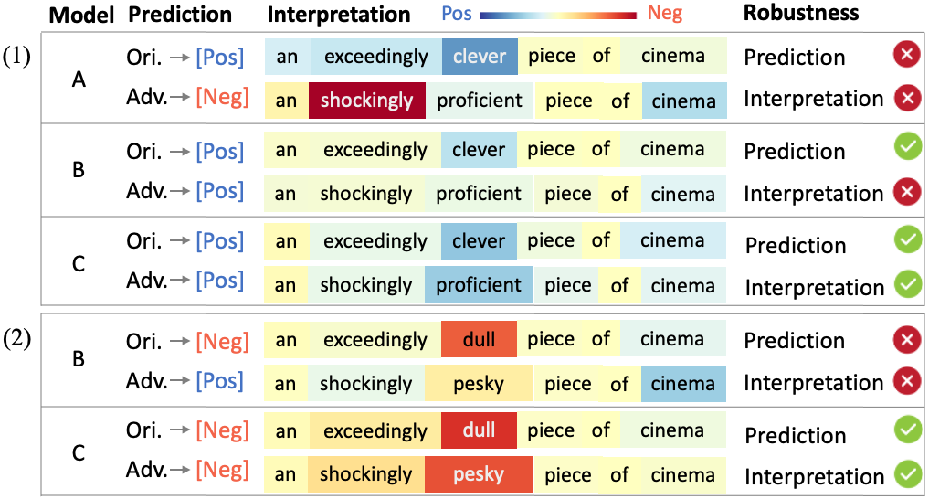
Figure 1: Illustration of different model robustness with respect to predictions and interpretations on (1) a positive movie review and (2) a negative movie review (Ori.), and their adversarial counterparts (Adv.). Model B makes the same correct predictions on Ori. and Adv. in (1), while the discrepant interpretations reveal its vulnerability which is attacked by another adversarial example in (2). Only model C is robust with the same predictions and consistent interpretations on both original/adversarial example pairs.

Previous methods on defending this kind of attacks via adversary detection and prevention (Zhou et al. 2019; Mozes et al. 2021) or certifiably robust training (Jia et al. 2019; Huang et al. 2019) either circumvent improving model predictions on adversarial examples or scale poorly to complex neural networks (Shi et al. 2020). Alternatively, adversarial training (Jin et al. 2020; Li et al. 2021) improves model robustness via two steps—collecting adversarial examples by attacking a target model, and fine-tuning the model on the augmented dataset with these adversarial examples. However, existing adversarial training only focuses on making a model produce the same correct predictions on an original/adversarial example pair, while ignores the consistency between model decision-makings on the two similar texts.

To illustrate the necessity of maintaining consistent model decision-makings (reflected by interpretations) during adversarial training, Fig. 1 shows both the predictions and their corresponding interpretations of different models on original/adversarial example pairs. The interpretations were generated by IG (Sundararajan, Taly, and Yan 2017), which visualizes the attribution of each input feature (word/token) to the model prediction. Figure 1 (1) shows the predictions and interpretations of model A, B, and C on a positive movie review and its adversarial counterpart. Model A is not robust as its prediction on the adversarial example is flipped and the interpretation is totally changed. Although model B makes the same predictions on the original and adversarial examples, its interpretations reveal that these predictions are based on different key features: for the original example, it is a sentiment word clever; for the adversarial example, it is a neutral word cinema. The interpretation discrepancy reveals the vulnerability of model B, as shown in Fig. 1 (2), where we craft another adversarial attack. Model B fails to recognize dull and pesky as the same important, and makes a wrong prediction on the negative adversarial example based on cinema. Only model C is robust as it behaves consistently on predicting both original/adversarial example pairs. Note that we look at model robustness through the lens of interpretations, while leaving the problem of trustworthiness or robustness of an interpretation method itself out as that is beyond the scope of this paper.

Based on the previous discussion, we argue that a robust model should have consistent prediction behaviors on original/adversarial example pairs, that is making the same predictions (what) based on the same reasons (how) which are reflected by consistent interpretations, as the word saliency maps of model C in Fig. 1. However, traditional adversarial training does not regularize model prediction behavior for improving model robustness. To train a robust model, we propose a fine-grained feature-level adversarial training named FLAT. FLAT learns global word importance via variational word masks (Chen and Ji 2020) and regularizes the importance scores of the replaced words and their substitutions in original/adversarial example pairs during training. FLAT teaches the model to behave consistently on predicting original/adversarial example pairs by focusing on the corresponding important words based on their importance scores, hence improving the model robustness to adversarial examples.

The contribution of this work is three-fold: (1) we argue that adversarial training should improve model robustness by making the model produce the same predictions on original/adversarial example pairs with consistent interpretations; (2) we propose a new training strategy, feature-level adversarial training (FLAT), to achieve this goal by regularizing model prediction behaviors on original/adversarial example pairs to be consistent; and (3) we evaluate the effectiveness of FLAT in improving the robustness of four neural network models, LSTM (Hochreiter and Schmidhuber 1997), CNN (Kim 2014), BERT (Devlin et al. 2019), and DeBERTa (He et al. 2021), to two adversarial attacks on four text classification tasks. The models trained via FLAT also show better robustness than baseline models on unforeseen adversarial examples across six different attacks.

2 Related Work

Neural language models have shown vulnerability to adversarial examples which are generated by manipulating input texts, such as replacing words with their synonyms (Alzantot et al. 2018; Ren et al. 2019; Jin et al. 2020; Li et al. 2021; Garg and Ramakrishnan 2020), introducing character typos (Li et al. 2018; Gao et al. 2018), paraphrasing sentences (Ribeiro, Singh, and Guestrin 2018; Iyyer et al. 2018), and inserting malicious triggers (Wallace et al. 2019). In this work, we focus on word substitution-based attacks as the generated adversarial examples largely maintain the original semantic meaning and lexical and grammatical correctness compared to other attacks (Zhang et al. 2020). Some methods defend this kind of attacks by detecting malicious inputs and preventing them from attacking a model (Zhou et al. 2019; Mozes et al. 2021; Wang et al. 2021). However, blocking adversaries does not essentially solve the vulnerability problem of the target model. Another line of works focus on improving model robustness, and broadly fall into two categories: (1) certifiably robust training and (2) adversarial training.

Certifiably robust training.

Jia et al. (2019); Huang et al. (2019) utilized interval bound propagation (IBP) to bound model robustness. Shi et al. (2020); Xu et al. (2020) extended the robustness verification to transformers, while it is challenging to scale these methods to complex neural networks (e.g. BERT) without loosening bounds. Ye, Gong, and Liu (2020) proposed a structure-free certified robust method which can be applied to advanced language models. However, the certified accuracy is at the cost of model performance on clean data.

Adversarial training.

Adversarial training in text domain usually follows two steps: (1) collecting adversarial examples by attacking a target model and (2) fine-tuning the model on the augmented dataset with these adversarial examples. The augmented adversarial examples can be real examples generated by perturbing the original texts (Jin et al. 2020; Li et al. 2021), produced by generation models (Wang et al. 2020), or virtual examples crafted from word embedding space by adding noise to original word embeddings (Miyato, Dai, and Goodfellow 2017; Zhu et al. 2020) or searching the worst-case in a convex hull (Zhou et al. 2021; Dong et al. 2021).

The above methods improve model robustness by solely looking at model predictions, that is making a model produce the same correct predictions on original/adversarial example pairs. Nevertheless, a robust model should behave consistently on predicting similar texts beyond producing the same predictions. Regularizing model prediction behavior should be considered in improving model robustness, no matter via certifiably robust training or adversarial training. In this work, we focus on extending traditional adversarial training to fine-grained feature-level adversarial training (FLAT), while leaving adding constraints on model behavior in certifiably robust training to future work. Besides, FLAT is compatible with existing substitution-based adversarial data augmentation methods. We focus on those (Jin et al. 2020; Ren et al. 2019) that generate adversarial examples by perturbing original texts in our experiments.

Another related work bounds model robustness by regularizing interpretation discrepancy between original and adversarial examples in image domain (Boopathy et al. 2020). However, the interpretations are post-hoc and could vary across different interpretation methods. Differently, FLAT learns global feature importance during training. By regularizing the global importance of replaced words and their substitutions, the model trained via FLAT would be robust to unforeseen adversarial examples in which the substitution words appear.

3 Method

This section introduces the proposed FLAT method. FLAT aims at improving model robustness by making a model behave consistently on predicting original/adversarial example pairs. To achieve this goal, FLAT leverages variational word masks to select the corresponding words (e.g. fantastic and marvelous in Fig. 2) from an original/adversarial example pair for the model to make predictions. To ensure the correctness of model predictions, variational word masks learn global word importance during training and play as a bottleneck teaching the model to make predictions based on important words. Besides, FLAT regularizes the global importance of the replaced words in an original example and their substitutions in the adversarial counterpart so that the model would recognize the corresponding words as the same important (or unimportant), as Fig. 2 shows.

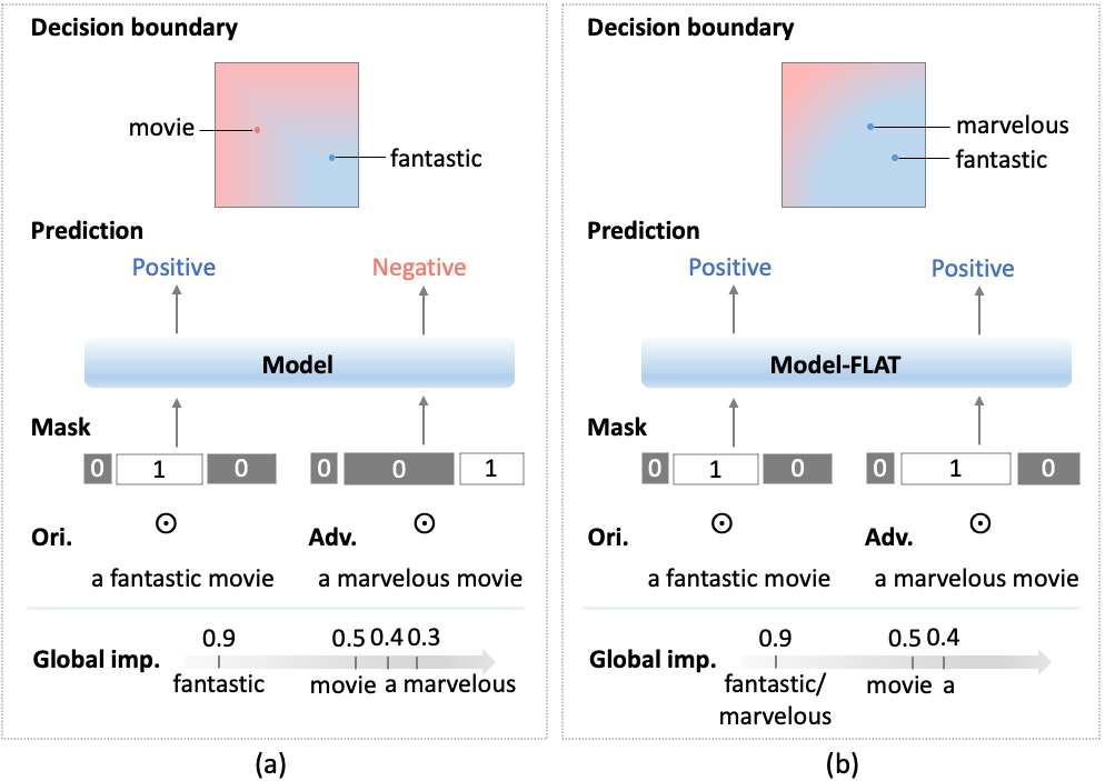
Figure 2: (a) The model with variational word masks trained on the standard training set. As marvelous is not recognized as the same important as its synonym fantastic and masked out, the model makes a wrong prediction based on a neutral word movie. (b) FLAT increases the global importance of marvelous and teaches the model to make the same correct predictions on the original/adversarial example pair by focusing on fantastic and marvelous respectively.

Preliminaries.

Given an input $\bm{x}=[\bm{x}_{1},\ldots,\bm{x}_{n}]$, where $\bm{x}_{i}\in\mathbb{R}^{d}$ ($i\in\{1,\dots,n\}$) denotes the word embedding, the model $f_{\bm{\theta}}(\cdot)$ with parameter $\bm{\theta}$ outputs a prediction label $y=f_{\bm{\theta}}(\bm{x})$ for text classification tasks. An adversarial example $\bm{x}^{\prime}$ is crafted from $\bm{x}$ under some constraints, such as maintaining the original semantic meaning. For word substitution-based adversarial attacks, an adversarial example replaces some words $\{\bm{x}_{i}\}$ in the original example $\bm{x}$ with their synonyms $\{\bm{x}^{\prime}_{i}\}$. The adversarial example fools the model to output a different label, i.e. $y^{\prime}=f_{\bm{\theta}}(\bm{x}^{\prime})\neq y$.

We obtain a set of adversarial examples $\mathcal{D}^{\prime}=\{(\bm{x}^{\prime(m)},y^{(m)})\}$ by attacking the model on the original dataset $\mathcal{D}=\{(\bm{x}^{(m)},y^{(m)})\}$. During adversarial training, the model is trained on both original and adversarial examples ($\mathcal{D}\cup\mathcal{D}^{\prime}$). In addition to improving model prediction accuracy on adversarial examples, adversarial training should also make the model produce the same predictions on the similar texts with consistent decision-makings. Failing to do this would make the model vulnerable to unforeseen adversarial examples crafted with the substitution words in some other contexts. To achieve this goal, we propose the feature-level adversarial training (FLAT) method.

3.1 Feature-Level Adversarial Training

Recall the goal of FLAT is to train a robust model with consistent prediction behaviors on original/adversarial example pairs. There are two desiderata for FLAT:

1. Global feature importance scores $\bm{\phi}$. To teach the model to recognize the replaced words in an original example and their substitutions in the adversarial counterpart as the same important (or unimportant) for predictions, FLAT needs to learn the global importance score $\phi_{\bm{x}_{i}}$ of a word $\bm{x}_{i}$. Note that the “global” means the importance score is solely dependent on the word (embedding).

2. Feature selection function $g_{\bm{\phi}}(\cdot)$. To guide the model to make predictions based on the corresponding important words in the original and adversarial example respectively, FLAT needs a feature selection function $g_{\bm{\phi}}(\cdot)$. $g_{\bm{\phi}}(\bm{x})$ selects important words from $\bm{x}$ based on their global importance scores in $\bm{\phi}$. The selected words are then forwarded to the model to output a prediction, i.e. $y=f_{\bm{\theta}}(g_{\bm{\phi}}(\bm{x}))$.

FLAT leverages variational word masks (Chen and Ji 2020) to learn global feature importance scores and select important features for model predictions, which will be introduced in Section 3.2.

With the two desiderata, the objective of FLAT is formulated as

$$\min_{\bm{\theta},\bm{\phi}} \mathcal{L}_{pred}+\gamma\mathcal{L}_{imp}$$ (1)

$$\mathcal{L}_{pred} =\mathop{\mathbb{E}}_{(\bm{x},y)\sim\mathcal{D}}[\mathcal{L}(f_{\bm{\theta}}(g_{\bm{\phi}}(\bm{x})),y)]$$

$$+\mathop{\mathbb{E}}_{(\bm{x}^{\prime},y)\sim\mathcal{D}^{\prime}}[\mathcal{L}(f_{\bm{\theta}}(g_{\bm{\phi}}(\bm{x}^{\prime})),y)]$$

$$\mathcal{L}_{imp} =\mathop{\mathbb{E}}_{(\bm{x},\bm{x}^{\prime})\sim\mathcal{D}\cup\mathcal{D}^{\prime}}[\sum_{i,\bm{x}_{i}\neq\bm{x}^{\prime}_{i}}\lvert\phi_{\bm{x}_{i}}-\phi_{\bm{x}^{\prime}_{i}}\rvert]$$ (3)

where $\mathcal{L}(\cdot,\cdot)$ denotes cross entropy loss. $\bm{\phi}$ is a learnable vector with the same dimension as the predefined vocabulary, where $\phi_{\bm{x}_{i}}\in(0,1)$ represents the global importance of the word $\bm{x}_{i}$. $\gamma\in\mathbb{R}_{+}$ is a coefficient. $\mathcal{L}_{imp}$ regularizes the global importance scores of the replaced words $\{\bm{x}_{i}\}$ and their substitutes $\{\bm{x}^{\prime}_{i}\}$ in an original/adversarial example pair $(\bm{x},\bm{x}^{\prime})$ by pushing $\phi_{\bm{x}_{i}}$ and $\phi_{\bm{x}^{\prime}_{i}}$ close. With similar importance scores, the associated word pair $(\bm{x}_{i},\bm{x}^{\prime}_{i})$ would be selected by $g_{\bm{\phi}}(\cdot)$ or not simultaneously. $\mathcal{L}_{pred}$ encourages the model to make the same and correct predictions on the original and adversarial example based on the selected important words $g_{\bm{\phi}}(\bm{x})$ and $g_{\bm{\phi}}(\bm{x}^{\prime})$ respectively. By optimizing the objective, the model learns to behave consistently on predicting similar texts, hence having better robustness to adversarial attacks.

3.2 Learning with Variational Word Masks

FLAT fulfills the two desiderata by training the model ($f_{\bm{\theta}}(\cdot)$) with variational word masks (Chen and Ji 2020). Specifically, variational word masks learn global word importance $\bm{\phi}$ during training and select important words for the model to make predictions by masking out irrelevant or unimportant words. For an input $\bm{x}=[\bm{x}_{1},\ldots,\bm{x}_{n}]$, a set of masks $\bm{W}=[W_{\bm{x}_{1}},\ldots,W_{\bm{x}_{n}}]$ are generated based on $\bm{\phi}$, where $W_{\bm{x}_{i}}\in\{0,1\}$ is a binary random variable with 0 and 1 indicating to mask out or select the word $\bm{x}_{i}$ respectively. The word importance score $\phi_{\bm{x}_{i}}$ is the expectation of $W_{\bm{x}_{i}}$, that is the probability of the word $\bm{x}_{i}$ being selected. The feature selection function $g_{\bm{\phi}}(\cdot)$ in Section 3.1 is defined as

$$g_{\bm{\phi}}(\bm{x})=\bm{W}\odot\bm{x},$$ (4)

where $\odot$ denotes element-wise multiplication.

To ensure the model concentrating on a few important words to make predictions, we regularize $\bm{W}$ by maximizing its entropy conditioned on $\bm{x}$. The intuition is that most words in the vocabulary are irrelevant or noisy features (e.g. stop words) to text classification tasks (Chen and Ji 2020). The regularization on $\bm{W}$ will push the importance scores of most irrelevant words close to 0.5, while making a few important words have relatively high importance scores (close to 1), and the rest unimportant words have low scores (close to 0). Under this constraint, we rewrite the prediction loss $\mathcal{L}_{pred}$ in the objective (1) as

$$\mathcal{L}_{pred}=\mathop{\mathbb{E}}_{(\bm{x},y)\sim\mathcal{D}}[\mathbb{E}_{q}[\mathcal{L}(f_{\bm{\theta}}(\bm{W}\odot\bm{x}),y)]-\beta H_{q}(\bm{W}\mid\bm{x})]$$

$$+\mathop{\mathbb{E}}_{(\bm{x}^{\prime},y)\sim\mathcal{D}^{\prime}}[\mathbb{E}_{q^{\prime}}[\mathcal{L}(f_{\bm{\theta}}(\bm{W}^{\prime}\odot\bm{x}^{\prime}),y)]-\beta H_{q^{\prime}}(\bm{W}^{\prime}\mid\bm{x}^{\prime})],$$

where $q=q_{\bm{\phi}}(\bm{W}\mid\bm{x})$ and $q^{\prime}=q_{\bm{\phi}}(\bm{W}^{\prime}\mid\bm{x}^{\prime})$ denote the distributions of word masks on the original example $\bm{x}$ and adversarial example $\bm{x}^{\prime}$ respectively, $H_{q}(\cdot\mid\cdot)$ is the conditional entropy, and $\beta\in\mathbb{R}_{+}$ is a coefficient.

3.3 Connection

FLAT degrades to traditional adversarial training when all words are regarded as equal important (all mask values are 1), and no constraint is added to regularize the importance scores of associated words in original/adversarial example pairs. Traditional adversarial training simply updates the model on the augmented dataset $\mathcal{D}\cup\mathcal{D}^{\prime}$ by optimizing

$$\min_{\bm{\theta}}\!\!\mathop{\mathbb{E}}_{(\bm{x},y)\sim\mathcal{D}}\!\![\mathcal{L}(f_{\bm{\theta}}(\bm{x}),y)]+\!\!\mathop{\mathbb{E}}_{(\bm{x}^{\prime},y)\sim\mathcal{D}^{\prime}}\!\![\mathcal{L}(f_{\bm{\theta}}(\bm{x}^{\prime})),y)].$$ (5)

With no constraint on model prediction behavior on predicting similar texts, the model robustness is not guaranteed, especially to unforeseen adversarial attacks, as the results shown in experiments.

3.4 Implementation Specification

We utilize the amortized variational inference (Kingma and Welling 2013) to approximate word mask distributions, and learn the parameter $\bm{\phi}$ (global word importance) via an inference network which is a single-layer feedforward neural network. For simplicity, we assume the word masks are mutually independent and each mask is dependent on the word embedding, that is $q_{\bm{\phi}}(\bm{W}\mid\bm{x})=\prod_{i=1}^{n}q_{\bm{\phi}}(W_{\bm{x}_{i}}\mid\bm{x}_{i})$. We optimize the inference network with the model jointly via stochastic gradient descent, and apply the Gumbel-softmax trick (Jang, Gu, and Poole 2017; Maddison, Mnih, and Teh 2016) to address the discreteness of sampling binary masks from Bernoulli distributions in backpropagation (Chen and Ji 2020). In the inference stage, we multiply each word embedding and its global importance score for the model to make predictions.

We first train a base model on the original dataset, and attack the model by manipulating the original training data and collect adversarial examples. Then we train the model on both original and adversarial examples via FLAT. We repeat the attacking and training processes 3-5 times (depending on the model and dataset) until convergence. Note that in each iteration, we augment the original training data with new adversarial examples generated by attacking the latest checkpoint.

4 Experimental Setup

The proposed method is evaluated with four neural network models in defending two adversarial attacks on four text classification tasks.

Datasets	C	L	#train	#dev	#test
SST2	2	19	6920	872	1821
IMDB	2	268	20K	5K	25K
AG	4	32	114K	6K	7.6K
TREC	6	10	5000	452	500

Table 1: Summary statistics of the datasets, where C is the number of classes, L is the average sentence length, # counts the number of examples in the train/dev/test sets.

Datasets.

The four text classification datasets are: Stanford Sentiment Treebank with binary labels SST2 (Socher et al. 2013), movie reviews IMDB (Maas et al. 2011), AG’s News (AG) (Zhang, Zhao, and LeCun 2015), and 6-class question classification TREC (Li and Roth 2002). For the datasets (e.g. IMDB) without standard train/dev/test split, we hold out a proportion of training examples as the development set. Table 1 shows the statistics of the datasets.

Models.

We evaluate the proposed method with a recurrent neural network (Hochreiter and Schmidhuber 1997, LSTM), a convolutional neural network (Kim 2014, CNN), and two state-of-the-art transformer-based models—BERT (Devlin et al. 2019) and DeBERTa (He et al. 2021). The LSTM and CNN are initialized with 300-dimensional pretrained word embeddings (Mikolov et al. 2013). We adopt the base versions of both BERT and DeBERTa.

Attack methods.

We adopt two adversarial attacks, Textfooler (Jin et al. 2020) and PWWS (Ren et al. 2019). Both methods check the lexical correctness and semantic similarity of adversarial examples with their original counterparts. The adversarial attacks are conducted on the TextAttack benchmark (Morris et al. 2020) with default settings. During adversarial training, we attack all training data for the SST2 and TREC datasets to collect adversarial examples, while randomly attacking 10K training examples for the IMDB and AG datasets due to computational costs.

More details of experimental setup are in Appendix A.

Models	SST2	IMDB	AG	TREC
LSTM-base	84.40	88.03	91.08	90.80
LSTM-adv(Textfooler)	82.32	88.79	90.29	87.60
LSTM-adv(PWWS)	82.59	88.37	91.16	89.60
LSTM-FLAT (Textfooler)	84.79	89.17	91.00	91.00
LSTM-FLAT (PWWS)	83.69	88.52	91.37	91.20
CNN-base	84.18	88.63	91.32	91.20
CNN-adv(Textfooler)	82.15	88.81	90.99	89.20
CNN-adv(PWWS)	83.42	88.89	91.30	90.00
CNN-FLAT (Textfooler)	83.09	88.89	91.64	89.20
CNN-FLAT (PWWS)	83.31	88.99	91.03	89.20
BERT-base	91.32	91.71	93.59	97.40
BERT-adv(Textfooler)	91.38	92.50	90.30	96.00
BERT-adv(PWWS)	90.88	93.14	93.38	95.20
BERT-FLAT (Textfooler)	91.54	92.78	94.07	96.20
BERT-FLAT (PWWS)	91.05	93.11	93.09	96.60
DeBERTa-base	94.18	93.80	93.62	96.40
DeBERTa-adv(Textfooler)	94.40	92.86	92.84	95.60
DeBERTa-adv(PWWS)	94.78	94.17	92.96	96.40
DeBERTa-FLAT (Textfooler)	94.29	94.29	94.29	96.40
DeBERTa-FLAT (PWWS)	94.12	94.26	93.82	96.40

Table 2: Prediction accuracy (%) of different models on standard test sets.

5 Results

We train the four models on the four datasets with different training strategies. The base model trained on the clean data is named with suffix “-base”. The model trained via traditional adversarial training is named with suffix “-adv”. The model trained via the proposed method is named with suffix “-FLAT”. For fairness, traditional adversarial training repeats the attacking and training processes the same times as FLAT. Table 2 shows the prediction accuracy of different models on standard test sets. The attack method used for generating adversarial examples during training is noted in brackets. For example, “CNN-FLAT (Textfooler)” means the CNN model trained via FLAT with adversarial examples generated by Textfooler attack. Different from previous defence methods (Jones et al. 2020; Zhou et al. 2021) that hurt model performance on clean data, adversarial training (“adv” and “FLAT”) does not cause significant model performance drop, and even improves prediction accuracy in some cases. Besides, we believe that producing high-quality adversarial examples for model training would further improve model prediction performance, and leave this to our future work. The rest of this section will focus on evaluating model robustness from both prediction and interpretation perspectives. The evaluation results are recorded in Table 3.

		SST2			IMDB			AG			TREC
Attacks	Models	AA	KT	TI	AA	KT	TI	AA	KT	TI	AA	KT	TI
Textfooler	LSTM-base	5.05	0.46	0.68	0.16	0.53	0.46	45.00	0.76	0.81	44.40	0.62	0.89
	LSTM-adv	12.36	0.49	0.68	29.18	0.60	0.58	48.39	0.76	0.82	51.20	0.51	0.87
	LSTM-FLAT	17.76	0.58	0.75	31.38	0.66	0.65	54.16	0.82	0.86	55.20	0.68	0.90
	CNN-base	1.98	0.46	0.69	3.72	0.64	0.56	8.74	0.55	0.62	45.20	0.68	0.91
	CNN-adv	2.53	0.52	0.72	16.04	0.71	0.65	15.84	0.55	0.62	52.60	0.71	0.92
	CNN-FLAT	37.07	0.70	0.82	32.62	0.76	0.75	25.18	0.61	0.67	62.20	0.87	0.96
	BERT-base	4.72	0.35	0.56	3.84	0.38	0.33	11.84	0.39	0.48	37.60	0.44	0.87
	BERT-adv	5.60	0.33	0.56	23.28	0.34	0.25	30.67	0.25	0.40	40.00	0.52	0.89
	BERT-FLAT	12.41	0.44	0.64	28.35	0.46	0.38	32.29	0.45	0.53	55.00	0.58	0.90
	DeBERTa-base	5.22	0.64	0.76	2.82	0.71	0.72	12.12	0.60	0.63	39.00	0.69	0.92
	DeBERTa-adv	7.96	0.60	0.73	8.38	0.81	0.77	25.70	0.61	0.62	42.80	0.69	0.93
	DeBERTa-FLAT	11.59	0.70	0.79	24.62	0.83	0.78	31.62	0.62	0.65	49.60	0.73	0.94
PWWS	LSTM-base	11.64	0.51	0.71	0.29	0.55	0.48	54.53	0.82	0.86	54.40	0.66	0.90
	LSTM-adv	18.73	0.57	0.74	23.68	0.63	0.61	61.17	0.84	0.88	64.20	0.61	0.88
	LSTM-FLAT	19.66	0.60	0.75	25.00	0.69	0.67	62.41	0.85	0.89	67.80	0.79	0.94
	CNN-base	8.29	0.53	0.72	4.36	0.72	0.59	18.86	0.57	0.64	54.20	0.71	0.91
	CNN-adv	12.63	0.57	0.73	20.64	0.72	0.68	33.21	0.56	0.63	63.00	0.76	0.92
	CNN-FLAT	14.83	0.58	0.74	20.70	0.73	0.69	71.37	0.91	0.93	65.60	0.77	0.93
	BERT-base	11.70	0.37	0.57	7.08	0.36	0.32	32.34	0.28	0.40	51.60	0.52	0.87
	BERT-adv	14.44	0.37	0.58	18.32	0.33	0.29	33.38	0.29	0.40	65.20	0.45	0.86
	BERT-FLAT	14.61	0.44	0.64	25.08	0.41	0.36	49.16	0.30	0.42	68.20	0.64	0.90
	DeBERTa-base	14.17	0.72	0.81	7.04	0.82	0.80	31.30	0.65	0.71	52.80	0.73	0.94
	DeBERTa-adv	15.16	0.65	0.76	18.66	0.81	0.78	53.02	0.65	0.70	63.60	0.64	0.91
	DeBERTa-FLAT	23.23	0.75	0.83	26.58	0.84	0.81	55.14	0.67	0.72	66.40	0.80	0.95

Table 3: Model robustness to adversarial attacks in terms of predictions and interpretations. AA: after-attack accuracy (%); KT: Kendall’s Tau order rank correlation; TI: top-k intersection ($k=5$).

5.1 Prediction Robustness

We evaluate the prediction robustness of well-trained models by attacking them with adversarial examples crafted from original test examples. The model prediction accuracy on adversarial examples is denoted as after-attack accuracy (Jin et al. 2020). In Table 3, we omit the attack name in naming a model (“-adv” or “-FLAT”) as it is trained with adversarial examples generated by the corresponding attack method (Textfooler or PWWS).

Table 3 shows that base models are easily fooled by adversarial examples, achieving much lower after-attack accuracy than other models (“-FLAT” and “-adv”) trained with adversarial examples. FLAT consistently outperforms traditional adversarial training, indicating the effectiveness of regularizing model prediction behavior during adversarial training in improving prediction robustness. All the models show better prediction robustness on multiclass topic classification tasks (AG and TREC) than on binary sentiment classification tasks (SST2 and IMDB). Besides, the after-attack accuracy on the IMDB dataset is the lowest for most of the base models (especially LSTM-base). We suspect that IMDB has longer average text length than other datasets, which is easier to find successful adversarial examples. FLAT improves the after-attack accuracy of base models $15\%-30\%$ on the IMDB dataset.

5.2 Interpretation Consistency

Beyond prediction robustness, model robustness can also be evaluated by comparing its decision-makings on predicting original/adversarial example pairs, i.e. interpretation consistency. Note that we obtain interpretations via local post-hoc interpretation methods that identify feature (word/token) attributions to the model prediction per example. We adopt two interpretation methods, IG (Sundararajan, Taly, and Yan 2017) and LIME (Ribeiro, Singh, and Guestrin 2016), which are the representatives from two typical categories, white-box interpretations and black-box interpretations, respectively. IG computes feature attributions by integrating gradients of points along a path from a baseline to the input. LIME explains neural network predictions by fitting a local linear model with input perturbations and producing word attributions. For IG, we evaluate all test examples and their adversarial counterparts. For LIME, we randomly pick up 1000 example pairs for evaluation due to computational costs. We evaluate interpretation consistency under two metrics, Kendall’s Tau order rank correlation (Chen et al. 2019; Boopathy et al. 2020) and Top-k intersection (Chen et al. 2019; Ghorbani, Abid, and Zou 2019). For both metrics, we compute the interpretation consistency on corresponding labels and take the average over all classes as the overall consistency. Table 3 reports the results of IG interpretations. The results of LIME interpretations (Table 8 in Appendix C) show similar tendency.

Kendall’s Tau order rank correlation.

We adopt this metric to compare the overall rankings of word attributions between different interpretations. Higher Kendall’s Tau order rank correlation indicates better interpretation consistency. The models (“-FLAT”) outperform other baseline models (“-adv” and “-base”) with higher Kendall’s Tau order rank correlations, showing that FLAT teaches models to behave consistently on predicting similar texts. However, traditional adversarial training cannot guarantee the model robustness being improved as the interpretation discrepancy is even worse than that of base models in some cases, such as LSTM-adv and LSTM-base on the TREC dataset under the Textfooler attack. As FLAT consistently improves model interpretation consistency, no matter which interpretation method (IG or LIME) is used for evaluation, we believe the model robustness has been improved.

Top-k intersection.

We adopt this metric to compute the proportion of intersection of top k important features identified by the interpretations of original/adversarial example pairs. Note that we treat synonyms as the ”same” words. Higher top-k intersection indicates better interpretation consistency. Table 3 records the results of IG interpretations when $k=5$. The full results of top-k intersection with k increasing from 1 to 10 are in Appendix C. Similar to the results of Kendall’s Tau order rank correlation, the models (“-FLAT”) outperform other baseline models (“-adv” and “-base”) with higher top-k intersection rates, showing that they tend to focus on the same words (or their synonyms) in original/adversarial example pairs to make predictions.

6 Discussion

Visualization of interpretations.

Interpretations show the robustness of models (“-FLAT”) in producing the same predictions on original/adversarial example pairs with consistent decision-makings. Figure 3 visualizes the IG interpretations of LSTM- and CNN-based models on a positive and negative SST2 movie review respectively. The adversarial examples of the two movie reviews were generated by Textfooler. The base models (“-base”) were fooled by adversarial examples. Although LSTM-adv correctly predicted the positive original/adversarial example pair, its interpretations are discrepant with treat and is identified as the top important word respectively. For the negative adversarial example, CNN-adv failed to recognize bad and wicked as synonyms and labeled them with opposite sentiment polarities, which explains its wrong prediction. Both LSTM-FLAT and CNN-FLAT correctly predicted the original/adversarial example pairs with consistent interpretations.

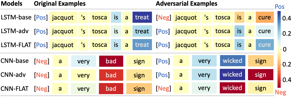
Figure 3: Visualization of IG interpretations. The model predictions are in “[ ]”. The color of each block represents the word attribution to the model prediction.

Models	PWWS	Gene	IGA	PSO	Clare	BAE
LSTM-base	11.64	20.26	9.83	5.88	3.02	36.52
LSTM-adv	15.38	25.65	17.02	5.60	3.90	36.35
LSTM-FLAT	20.48	33.44	24.22	6.53	5.55	39.87
CNN-base	8.29	20.32	7.85	5.60	1.48	37.12
CNN-adv	8.68	16.42	6.26	5.60	1.04	35.48
CNN-FLAT	42.56	55.02	46.35	10.38	17.57	48.38
BERT-base	11.70	32.24	9.72	6.26	0.86	35.31
BERT-adv	13.01	34.49	10.87	6.64	1.04	36.74
BERT-FLAT	15.93	35.31	15.93	9.50	5.29	37.56
DeBERTa-base	14.17	37.12	12.19	6.75	0.55	38.61
DeBERTa-adv	17.52	37.18	12.85	7.96	1.07	40.14
DeBERTa-FLAT	21.80	48.16	28.17	13.01	1.37	44.54

Table 4: After-attack accuracy (%) of different models to different attacks on the SST2 test set.

Transferability of model robustness.

The models trained via FLAT show better robustness than baseline models across different attacks. We test the robustness transferability of different models, where “-adv” and “FLAT” were trained with adversarial examples generated by Textfooler, to six unforeseen adversarial attacks: PWWS (Ren et al. 2019), Gene (Alzantot et al. 2018), IGA (Wang, Jin, and He 2019), PSO (Zang et al. 2020), Clare (Li et al. 2021), and BAE (Garg and Ramakrishnan 2020), which generate adversarial examples in different ways (e.g. WordNet swap (Miller 1998), BERT masked token prediction). The details of these attack methods are in Appendix A. Table 4 shows the after-attack accuracy of different models on the SST2 test set. The models trained via FLAT achieve higher after-attack accuracy than baseline models, showing better robustness to unforeseen adversarial examples.

Ablation study.

The regularizations on word masks and global word importance scores in the objective (1) are important for improving model performance. We take the LSTM-FLAT model trained with Textfooler adversarial examples on the SST2 dataset for evaluation. The optimal hyperparameters are $\beta=0.1$, $\gamma=0.001$. We study the effects by setting $\beta$, $\gamma$, or both as zero. Table 5 shows the results. Only with both regularizations, the model can achieve good prediction performance on the clean test data (standard accuracy) and adversarial examples (after-attack accuracy). We observed that when $\beta=0$, all masks are close to 1, failing to learn feature importance. When $\gamma=0$, the model cannot recognize some words and their substitutions as the same important, which is reflected by the larger variance of L1 norm on the difference between the global importance of 1000 randomly sampled words and 10 of their synonyms, as Fig. 5 shows in Appendix D.

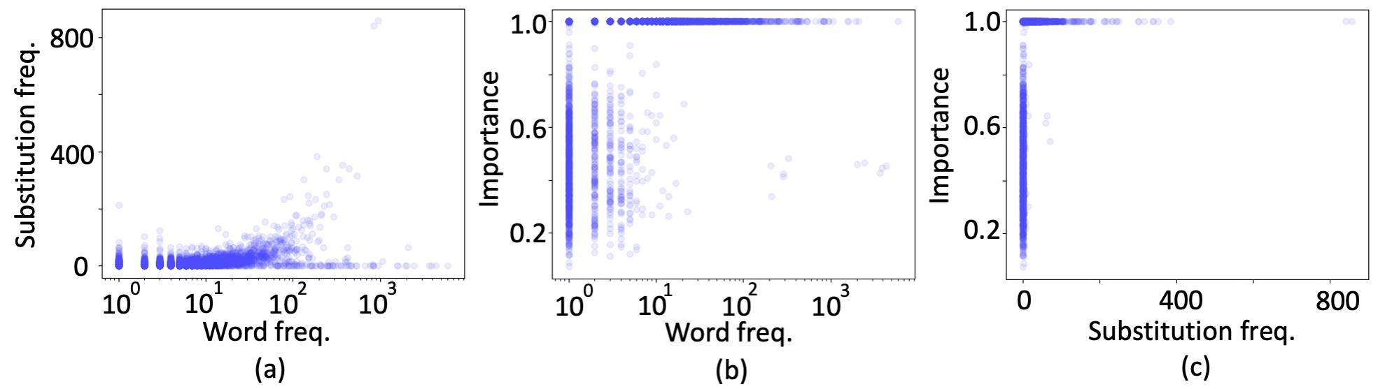
Figure 4: Scatter plots: (a) substitution frequency vs. word frequency; (b) global importance vs. word frequency; (c) global importance vs. substitution frequency.

Hyperparameters	SA	AA
$\beta=0.1$, $\gamma=0.001$	84.79	17.76
$\beta=0.1$, $\gamma=0$	83.96	9.99
$\beta=0$, $\gamma=0.001$	84.34	8.18
$\beta=0$, $\gamma=0$	84.40	8.35

Table 5: The effects of FLAT regularizations on model performance. SA: standard accuracy (%); AA: after-attack accuracy (%)

Correlations.

The learned global word importance, word frequency, and word substitution frequency in adversarial examples do not show strong correlations with each other. We take the LSTM-FLAT trained with Textfooler on the SST2 dataset for analysis. As the scatter plots in Fig. 4 show, any two of the three do not have strong correlations (as their Pearson correlations show in Table 9 in Appendix D). Figure 4 (a) shows that the replaced words are not based on their frequency. Figure 4 (b) and (c) show that global word importance scores were learned during training, not trivially based on word frequency or substitution frequency. It is expected the words that have high substitution frequency in adversarial examples have high importance scores. In addition, FLAT also identifies some important words that are low-frequency or even not replaced by adversarial examples.

7 Conclusion

In this paper, we look into the robustness of neural network models from both prediction and interpretation perspectives. We propose a new training strategy, FLAT, to regularize a model prediction behavior so that it produces the same predictions on original/adversarial example pairs with consistent interpretations. We test FLAT with four neural network models, LSTM, CNN, BERT, and DeBERTa, and show its effectiveness in improving model robustness to two adversarial attacks on four text classification tasks.

Appendix A Supplement of Experimental Setup

Models.

The CNN model (Kim 2014) contains a single convolutional layer with filter sizes ranging from 3 to 5. The LSTM (Hochreiter and Schmidhuber 1997) has a single unidirectional hidden layer. We adopt the pretrained BERT-base and DeBERTa-base models from Hugging Face. We implement the models in PyTorch 1.7.

Datasets.

We clean up the text by converting all characters to lowercase, removing extra whitespaces and special characters. We tokenize texts and remove low-frequency words to build vocab. We truncate or pad sentences to the same length for mini-batch during training. Table 6 shows pre-processing details on the datasets.

Datasets	$vocab$	$threshold$	$length$
SST2	13838	0	50
IMDB	29571	5	250
AG	21821	5	50
TREC	8095	0	15

Table 6: Pre-processing details on the datasets. $vocab$: vocab size; $threshold$: low-frequency threshold; $length$: mini-batch sentence length.

Attack methods.

We conducted all the adversarial attacks on the TextAttack benchmark (Morris et al. 2020) with default settings.

1. Textfooler (Jin et al. 2020): Textfooler generates adversarial examples by replacing important words with synonyms from the counter-fitting word embedding space (Mrkšić et al. 2016). Part-of-speech (POS) checking and semantic similarity checking via Universal Sentence Encoder (USE) are adopted to select high-quality adversarial examples.

2. PWWS (Ren et al. 2019): PWWS generates adversarial examples by replacing words with their synonyms in WordNet (Miller 1998) and replacing named entities (NEs) with similar NEs.

3. Gene (Alzantot et al. 2018): Gene perturbs percentage of words with their nearest neighbors in the GloVe embedding space (Pennington, Socher, and Manning 2014) and generates adversarial examples via genetic algorithms.

4. IGA (Wang, Jin, and He 2019): IGA is an improved genetic based text attack method (Alzantot et al. 2018) which allows to substitute a word with their synonyms in the same position more than once.

5. PSO (Zang et al. 2020): PSO generates adversarial examples by swapping words from HowNet (Dong, Dong, and Hao 2010).

6. Clare (Li et al. 2021): Clare is a context-aware adversarial attack method. It applies masks on inputs and plugs in an alternative using a pretrained masked language model RoBERTa (Liu et al. 2019).

7. BAE (Garg and Ramakrishnan 2020): BAE replaces and inserts tokens in the original text by masking a portion of the text and leveraging a BERT masked language model to generate alternatives for the masked tokens.

All experiments were performed on a single NVidia GTX 1080 GPU.

Appendix B Validation Performance

The corresponding validation accuracy for each reported test accuracy is in Table 7.

Models	SST2	IMDB	AG	TREC
LSTM-base	85.21	88.42	90.68	89.16
LSTM-adv(Textfooler)	83.95	88.52	89.63	88.72
LSTM-adv(PWWS)	83.49	88.56	90.97	87.39
LSTM-FLAT (Textfooler)	84.29	89.02	90.70	89.38
LSTM-FLAT (PWWS)	84.52	88.60	91.25	90.27
CNN-base	84.06	88.50	90.97	88.27
CNN-adv(Textfooler)	82.22	88.94	91.07	88.05
CNN-adv(PWWS)	82.91	88.84	91.03	89.16
CNN-FLAT (Textfooler)	83.72	88.78	91.40	88.70
CNN-FLAT (PWWS)	82.22	88.90	90.93	88.05
BERT-base	91.63	85.52	94.63	94.25
BERT-adv(Textfooler)	91.97	87.16	90.48	94.47
BERT-adv(PWWS)	90.67	94.02	94.52	94.47
BERT-FLAT (Textfooler)	91.40	87.32	94.80	94.91
BERT-FLAT (PWWS)	91.74	87.28	94.23	94.69
DeBERTa-base	93.81	88.64	94.25	94.69
DeBERTa-adv(Textfooler)	93.92	87.64	94.47	95.13
DeBERTa-adv(PWWS)	94.04	89.16	94.50	92.13
DeBERTa-FLAT (Textfooler)	93.46	89.52	94.73	94.69
DeBERTa-FLAT (PWWS)	93.35	89.44	94.68	95.13

Table 7: Validation accuracy (%) for each reported test accuracy.

Appendix C Supplement of Quantitative Evaluations

The results of model robustness with respect to LIME interpretations are in Table 8, showing the same tendency as those of IG interpretations reported in Table 3.

		SST2		IMDB		AG		TREC
Attacks	Models	KT	TI	KT	TI	KT	TI	KT	TI
Textfooler	LSTM-base	0.33	0.65	0.39	0.50	0.27	0.41	0.20	0.83
	LSTM-adv	0.36	0.67	0.39	0.53	0.25	0.39	0.36	0.83
	LSTM-FLAT	0.39	0.69	0.41	0.54	0.41	0.52	0.45	0.87
	CNN-base	0.33	0.67	0.44	0.51	0.25	0.37	0.27	0.83
	CNN-adv	0.35	0.68	0.46	0.53	0.25	0.38	0.32	0.84
	CNN-FLAT	0.39	0.69	0.50	0.56	0.26	0.40	0.40	0.87
	BERT-base	0.14	0.55	0.13	0.20	0.07	0.23	0.08	0.79
	BERT-adv	0.13	0.54	0.10	0.17	0.07	0.23	0.10	0.79
	BERT-FLAT	0.21	0.60	0.14	0.21	0.11	0.25	0.12	0.81
	DeBERTa-base	0.21	0.55	0.17	0.25	0.08	0.23	0.13	0.81
	DeBERTa-adv	0.20	0.54	0.12	0.19	0.08	0.23	0.13	0.81
	DeBERTa-FLAT	0.22	0.56	0.19	0.26	0.09	0.24	0.14	0.82
PWWS	LSTM-base	0.36	0.67	0.39	0.52	0.26	0.41	0.19	0.82
	LSTM-adv	0.38	0.68	0.35	0.52	0.26	0.41	0.22	0.82
	LSTM-FLAT	0.42	0.71	0.40	0.55	0.27	0.43	0.25	0.83
	CNN-base	0.37	0.68	0.43	0.52	0.26	0.39	0.19	0.83
	CNN-adv	0.43	0.71	0.47	0.54	0.26	0.41	0.22	0.84
	CNN-FLAT	0.47	0.73	0.51	0.55	0.27	0.42	0.25	0.85
	BERT-base	0.14	0.55	0.13	0.21	0.07	0.22	0.08	0.79
	BERT-adv	0.11	0.54	0.11	0.17	0.07	0.22	0.11	0.79
	BERT-FLAT	0.25	0.60	0.24	0.31	0.08	0.24	0.13	0.80
	DeBERTa-base	0.22	0.55	0.16	0.23	0.08	0.23	0.12	0.80
	DeBERTa-adv	0.18	0.53	0.15	0.21	0.08	0.23	0.12	0.80
	DeBERTa-FLAT	0.23	0.57	0.19	0.25	0.09	0.24	0.13	0.81

Table 8: Model robustness to adversarial attacks in terms of LIME interpretations. KT: Kendall’s Tau order rank correlation; TI: top-k intersection ($k=5$).

The top-k intersections of IG interpretations under the Textfooler attack with k increasing from 1 to 10 are shown in Fig. 6.

Appendix D Supplement of Discussion

Ablation study.

To evaluate the effect of the regularization on global importance scores of the replaced words and their substitutions, we compare the LSTM-FLAT model trained with parameters $\beta=0.1$, $\gamma=0.001$ and the other one trained with $\beta=0.1$, $\gamma=0$. Fig. 5 shows the box plot of L1 norm on the difference between the learned global importance of 1000 randomly sampled words and 10 of their synonyms in the counter-fitting word embedding space (Mrkšić et al. 2016). The results show that the model trained without the regularization ($\beta=0.1$, $\gamma=0$) has larger variance on the global importance scores of synonyms, which makes the model fail to recognize some words and their substitutions as the same important, resulting in relatively low after-attack accuracy.

Correlations between global word importance, word frequency, and word substitution frequency.

The scatter plots in Fig. 4 show the correlations between global word importance, word frequency, and word substitution frequency of LSTM-FLAT on the SST2 dataset. Any two of the three do not have strong correlations, as their Pearson correlations show in Table 9. Figure 4 (a) shows that adversarial examples attack the model vulnerability by replacing some words in original input texts, while the replaced words are not based on their frequency. Figure 4 (b) and (c) show that global word importance scores were learned during training, not trivially based on word frequency or substitution frequency. It is obvious the words that have high substitution frequency in adversarial examples have high importance scores. FLAT can also recognize important words with low frequency or even not replaced as they are important for model predictions.

Correlation	Coefficient r	P-value
WI - WF	-0.028	0.001
WI - SF	0.087	5.79e-5
WF - SF	0.162	1.65e-8

Table 9: Pearson correlations between global word importance (WI), word frequency (WF), and word substitution frequency (SF).

A trivial case of FLAT.

FLAT automatically learns global word importance and regularizes the importance between word pairs based on the model vulnerability detected by adversarial examples, rather than simply giving the same importance to synonyms. We designed a trivial method for comparison in our pilot experiments. Specifically, we cluster similar words into different groups based on their distance in the counter-fitting word embedding space (Mrkšić et al. 2016). Each group of words share the same mask with the value initialized as 1. We train a CNN model with the group masks which are applied on word embeddings on the AG dataset. We test the model robustness with Textfooler attack.

Table 10 shows model performance with different predefined group numbers. This trivial method can not help improve model prediction performance on either the standard test set or adversarial examples, even with the number of groups increased. Besides, the embedding space used for clustering words is specified and the number of clusters is predefined, which limit the applicability of this method to defend more complex adversarial attacks. Motivated by these observations, we proposed FLAT to automatically learn and adjust word importance for improving model robustness via adversarial training.

Group number	SA	AA
10	91.13	1.20
20	90.97	1.92
30	91.13	1.40
40	91.13	1.46
50	91.09	1.38

Table 10: Model performance with different group numbers. SA: standard accuracy (%); AA: after-attack accuracy (%)

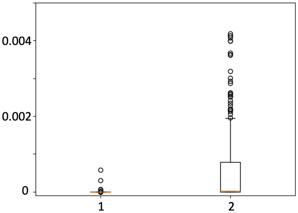
Figure 5: Box plot of the L1 norm on the difference between the global importance scores of 1000 randomly sampled words and 10 of their synonyms. 1: $\beta=0.1$, $\gamma=0.001$; 2: $\beta=0.1$, $\gamma=0$.

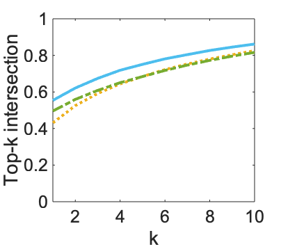
(a) LSTM, SST2

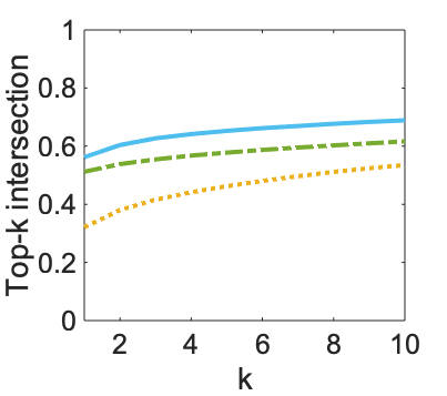
(b) LSTM, IMDB

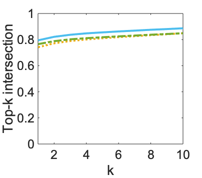
(c) LSTM, AG

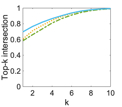
(d) LSTM, TREC

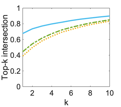
(e) CNN, SST2

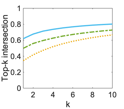
(f) CNN, IMDB

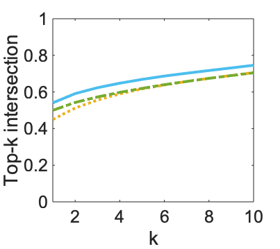
(g) CNN, AG

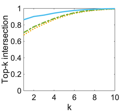
(h) CNN, TREC

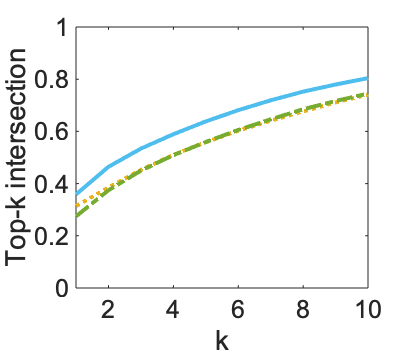
(i) BERT, SST2

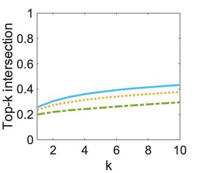
(j) BERT, IMDB

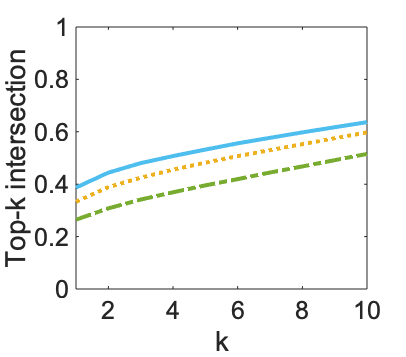
(k) BERT, AG

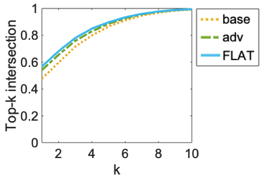
(l) BERT, TREC

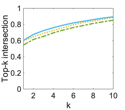
(m) DeBERTa, SST2

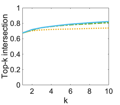
(n) DeBERTa, IMDB

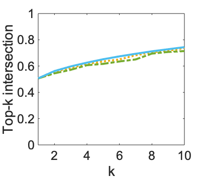
(o) DeBERTa, AG

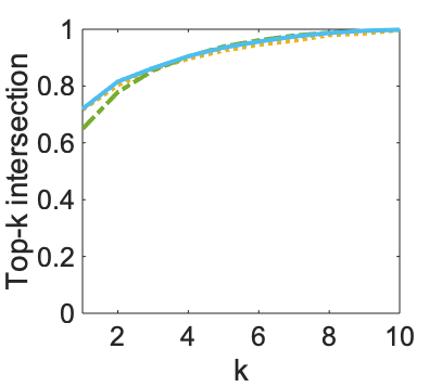
(p) DeBERTa, TREC

Figure 6: Top-k intersection of IG interpretations for different models on the four datasets under the Textfooler attack with k increasing from 1 to 10.

Appendix E Hyperparameters for Reproduction

We tune hyperparameters manually for each model to achieve the best prediction accuracy on standard test sets. We experiment with different hyperparameters, such as learning rate $lr\in\{1e-5,1e-3,\cdots,0.1\}$, clipping norm $clip\in\{1e-3,1e-2,\cdots,1,5,10\}$, $\beta\in\{0.00001,0.1,\cdots,1000\}$, and $\gamma\in\{0.00001,0.1,\cdots,1000\}$. All reported results are based on one run for each setting.

References

- Alzantot et al. (2018) Alzantot, M.; Sharma, Y.; Elgohary, A.; Ho, B.-J.; Srivastava, M.; and Chang, K.-W. 2018. Generating Natural Language Adversarial Examples. In EMNLP.
- Boopathy et al. (2020) Boopathy, A.; Liu, S.; Zhang, G.; Liu, C.; Chen, P.-Y.; Chang, S.; and Daniel, L. 2020. Proper Network Interpretability Helps Adversarial Robustness in Classification. In ICML, 1014–1023. PMLR.
- Chen and Ji (2020) Chen, H.; and Ji, Y. 2020. Learning Variational Word Masks to Improve the Interpretability of Neural Text Classifiers. In EMNLP.
- Chen et al. (2019) Chen, J.; Wu, X.; Rastogi, V.; Liang, Y.; and Jha, S. 2019. Robust attribution regularization. In NeurIPS.
- Devlin et al. (2019) Devlin, J.; Chang, M.-W.; Lee, K.; and Toutanova, K. 2019. Bert: Pre-training of deep bidirectional transformers for language understanding. In NAACL-HLT.
- Dong et al. (2021) Dong, X.; Luu, A. T.; Ji, R.; and Liu, H. 2021. Towards robustness against natural language word substitutions. In ICLR.
- Dong, Dong, and Hao (2010) Dong, Z.; Dong, Q.; and Hao, C. 2010. HowNet and Its Computation of Meaning. In Coling 2010: Demonstrations.
- Gao et al. (2018) Gao, J.; Lanchantin, J.; Soffa, M. L.; and Qi, Y. 2018. Black-box generation of adversarial text sequences to evade deep learning classifiers. In 2018 IEEE SPW.
- Garg and Ramakrishnan (2020) Garg, S.; and Ramakrishnan, G. 2020. BAE: BERT-based Adversarial Examples for Text Classification. In EMNLP.
- Ghorbani, Abid, and Zou (2019) Ghorbani, A.; Abid, A.; and Zou, J. 2019. Interpretation of neural networks is fragile. In AAAI.
- He et al. (2021) He, P.; Liu, X.; Gao, J.; and Chen, W. 2021. Deberta: Decoding-enhanced bert with disentangled attention. In ICLR.
- Hochreiter and Schmidhuber (1997) Hochreiter, S.; and Schmidhuber, J. 1997. Long short-term memory. Neural computation, 9(8): 1735–1780.
- Huang et al. (2019) Huang, P.-S.; Stanforth, R.; Welbl, J.; Dyer, C.; Yogatama, D.; Gowal, S.; Dvijotham, K.; and Kohli, P. 2019. Achieving Verified Robustness to Symbol Substitutions via Interval Bound Propagation. In EMNLP-IJCNLP.
- Iyyer et al. (2018) Iyyer, M.; Wieting, J.; Gimpel, K.; and Zettlemoyer, L. 2018. Adversarial Example Generation with Syntactically Controlled Paraphrase Networks. In NAACL-HLT.
- Jang, Gu, and Poole (2017) Jang, E.; Gu, S.; and Poole, B. 2017. Categorical reparameterization with gumbel-softmax. In ICLR.
- Jia et al. (2019) Jia, R.; Raghunathan, A.; Göksel, K.; and Liang, P. 2019. Certified Robustness to Adversarial Word Substitutions. In EMNLP-IJCNLP.
- Jin et al. (2020) Jin, D.; Jin, Z.; Zhou, J. T.; and Szolovits, P. 2020. Is bert really robust? a strong baseline for natural language attack on text classification and entailment. In AAAI.
- Jones et al. (2020) Jones, E.; Jia, R.; Raghunathan, A.; and Liang, P. 2020. Robust Encodings: A Framework for Combating Adversarial Typos. In ACL.
- Kim (2014) Kim, Y. 2014. Convolutional Neural Networks for Sentence Classification. In EMNLP.
- Kingma and Welling (2013) Kingma, D. P.; and Welling, M. 2013. Auto-encoding variational bayes. arXiv preprint arXiv:1312.6114.
- Li et al. (2021) Li, D.; Zhang, Y.; Peng, H.; Chen, L.; Brockett, C.; Sun, M.-T.; and Dolan, B. 2021. Contextualized Perturbation for Textual Adversarial Attack. In NAACL-HLT.
- Li et al. (2018) Li, J.; Ji, S.; Du, T.; Li, B.; and Wang, T. 2018. Textbugger: Generating adversarial text against real-world applications. arXiv preprint arXiv:1812.05271.
- Li and Roth (2002) Li, X.; and Roth, D. 2002. Learning question classifiers. In Proceedings of the 19th international conference on Computational linguistics-Volume 1, 1–7. Association for Computational Linguistics.
- Liang et al. (2017) Liang, B.; Li, H.; Su, M.; Bian, P.; Li, X.; and Shi, W. 2017. Deep text classification can be fooled. arXiv preprint arXiv:1704.08006.
- Liu et al. (2019) Liu, Y.; Ott, M.; Goyal, N.; Du, J.; Joshi, M.; Chen, D.; Levy, O.; Lewis, M.; Zettlemoyer, L.; and Stoyanov, V. 2019. Roberta: A robustly optimized bert pretraining approach. arXiv preprint arXiv:1907.11692.
- Maas et al. (2011) Maas, A. L.; Daly, R. E.; Pham, P. T.; Huang, D.; Ng, A. Y.; and Potts, C. 2011. Learning word vectors for sentiment analysis. In ACL.
- Maddison, Mnih, and Teh (2016) Maddison, C. J.; Mnih, A.; and Teh, Y. W. 2016. The concrete distribution: A continuous relaxation of discrete random variables. arXiv preprint arXiv:1611.00712.
- Mikolov et al. (2013) Mikolov, T.; Sutskever, I.; Chen, K.; Corrado, G. S.; and Dean, J. 2013. Distributed representations of words and phrases and their compositionality. In Advances in neural information processing systems, 3111–3119.
- Miller (1998) Miller, G. A. 1998. WordNet: An electronic lexical database. MIT press.
- Miyato, Dai, and Goodfellow (2017) Miyato, T.; Dai, A. M.; and Goodfellow, I. 2017. Adversarial training methods for semi-supervised text classification. In Proceedings of the International Conference on Learning Representations.
- Morris et al. (2020) Morris, J.; Lifland, E.; Yoo, J. Y.; Grigsby, J.; Jin, D.; and Qi, Y. 2020. TextAttack: A Framework for Adversarial Attacks, Data Augmentation, and Adversarial Training in NLP. In Proceedings of the 2020 Conference on Empirical Methods in Natural Language Processing: System Demonstrations, 119–126.
- Mozes et al. (2021) Mozes, M.; Stenetorp, P.; Kleinberg, B.; and Griffin, L. 2021. Frequency-Guided Word Substitutions for Detecting Textual Adversarial Examples. In Proceedings of the 16th Conference of the European Chapter of the Association for Computational Linguistics: Main Volume, 171–186. Online: Association for Computational Linguistics.
- Mrkšić et al. (2016) Mrkšić, N.; Séaghdha, D. O.; Thomson, B.; Gašić, M.; Rojas-Barahona, L.; Su, P.-H.; Vandyke, D.; Wen, T.-H.; and Young, S. 2016. Counter-fitting word vectors to linguistic constraints. arXiv preprint arXiv:1603.00892.
- Pennington, Socher, and Manning (2014) Pennington, J.; Socher, R.; and Manning, C. 2014. GloVe: Global Vectors for Word Representation. In EMNLP.
- Ren et al. (2019) Ren, S.; Deng, Y.; He, K.; and Che, W. 2019. Generating natural language adversarial examples through probability weighted word saliency. In ACL.
- Ribeiro, Singh, and Guestrin (2016) Ribeiro, M. T.; Singh, S.; and Guestrin, C. 2016. ” Why should i trust you?” Explaining the predictions of any classifier. In Proceedings of the 22nd ACM SIGKDD international conference on knowledge discovery and data mining, 1135–1144.
- Ribeiro, Singh, and Guestrin (2018) Ribeiro, M. T.; Singh, S.; and Guestrin, C. 2018. Semantically Equivalent Adversarial Rules for Debugging NLP models. In ACL.
- Samanta and Mehta (2017) Samanta, S.; and Mehta, S. 2017. Towards crafting text adversarial samples. arXiv preprint arXiv:1707.02812.
- Shi et al. (2020) Shi, Z.; Zhang, H.; Chang, K.-W.; Huang, M.; and Hsieh, C.-J. 2020. Robustness verification for transformers. arXiv preprint arXiv:2002.06622.
- Socher et al. (2013) Socher, R.; Perelygin, A.; Wu, J.; Chuang, J.; Manning, C. D.; Ng, A.; and Potts, C. 2013. Recursive deep models for semantic compositionality over a sentiment treebank. In EMNLP.
- Sundararajan, Taly, and Yan (2017) Sundararajan, M.; Taly, A.; and Yan, Q. 2017. Axiomatic attribution for deep networks. In International Conference on Machine Learning, 3319–3328. PMLR.
- Wallace et al. (2019) Wallace, E.; Feng, S.; Kandpal, N.; Gardner, M.; and Singh, S. 2019. Universal adversarial triggers for attacking and analyzing NLP. arXiv preprint arXiv:1908.07125.
- Wang et al. (2020) Wang, T.; Wang, X.; Qin, Y.; Packer, B.; Li, K.; Chen, J.; Beutel, A.; and Chi, E. 2020. CAT-Gen: Improving Robustness in NLP Models via Controlled Adversarial Text Generation. In EMNLP.
- Wang, Jin, and He (2019) Wang, X.; Jin, H.; and He, K. 2019. Natural language adversarial attacks and defenses in word level. arXiv preprint arXiv:1909.06723.
- Wang et al. (2021) Wang, X.; Jin, H.; Yang, Y.; and He, K. 2021. Natural Language Adversarial Defense through Synonym Encoding. In UAI.
- Xu et al. (2020) Xu, K.; Shi, Z.; Zhang, H.; Wang, Y.; Chang, K.-W.; Huang, M.; Kailkhura, B.; Lin, X.; and Hsieh, C.-J. 2020. Automatic perturbation analysis for scalable certified robustness and beyond. Advances in Neural Information Processing Systems, 33.
- Ye, Gong, and Liu (2020) Ye, M.; Gong, C.; and Liu, Q. 2020. SAFER: A Structure-free Approach for Certified Robustness to Adversarial Word Substitutions. In ACL.
- Zang et al. (2020) Zang, Y.; Qi, F.; Yang, C.; Liu, Z.; Zhang, M.; Liu, Q.; and Sun, M. 2020. Word-level Textual Adversarial Attacking as Combinatorial Optimization. In ACL.
- Zhang et al. (2020) Zhang, W. E.; Sheng, Q. Z.; Alhazmi, A.; and Li, C. 2020. Adversarial attacks on deep-learning models in natural language processing: A survey. ACM Transactions on Intelligent Systems and Technology (TIST), 11(3): 1–41.
- Zhang, Zhao, and LeCun (2015) Zhang, X.; Zhao, J.; and LeCun, Y. 2015. Character-level convolutional networks for text classification. In Advances in neural information processing systems, 649–657.
- Zhou et al. (2019) Zhou, Y.; Jiang, J.-Y.; Chang, K.-W.; and Wang, W. 2019. Learning to Discriminate Perturbations for Blocking Adversarial Attacks in Text Classification. In EMNLP-IJCNLP.
- Zhou et al. (2021) Zhou, Y.; Zheng, X.; Hsieh, C.-J.; Chang, K.-W.; and Huang, X. 2021. Defense against Synonym Substitution-based Adversarial Attacks via Dirichlet Neighborhood Ensemble. In ACL.
- Zhu et al. (2020) Zhu, C.; Cheng, Y.; Gan, Z.; Sun, S.; Goldstein, T.; and Liu, J. 2020. Freelb: Enhanced adversarial training for language understanding. In Proceedings of the International Conference on Learning Representations.