Abstract

The measurement of the triple Higgs coupling is one of the main tasks of the (HL-)LHC and future lepton colliders. Similarly, triple Higgs couplings involving BSM Higgs bosons are of high interest. Within the framework of Two Higgs Doublet Models (2HDM) we investigate the allowed ranges for all triple Higgs couplings involving at least one light, SM-like Higgs boson. We present newly the allowed ranges for 2HDM type III and IV and update the results within the type I and II. We take into account theoretical constraints from unitarity and stability, experimental constraints from direct BSM Higgs-boson searches, measurements of the rates of the SM-like Higgs-boson at the LHC, as well as flavor observables and electroweak precision data. For the SM-type triple Higgs coupling w.r.t. its SM value, $\lambda_{hhh}/\lambda_{\mathrm{SM}}$, we find allowed intervals of $\sim[-0.5,1.3]$ in type I and $\sim[0.5,1.0]$ in the other Yukawa types. These allowed ranges have important implications for the experimental determination of this coupling at future collider experiments. We find the coupling $\lambda_{hhH}$ between $\sim-1.5$ and $\sim+1.5$ in the four Yukawa types. For the triple Higgs couplings involving two heavy neutral Higgs bosons, $\lambda_{hHH}$ and $\lambda_{hAA}$ we find values between $\sim-0.5$ and $\sim 16$, and between $\sim-1$ and $\sim 32$ for $\lambda_{hH^{+}H^{-}}$. These potentially large values could lead to strongly enhanced production of two Higgs-bosons at the HL-LHC or high-energy lepton colliders.

1 Introduction

The discovery of a new scalar particle with a mass of $\sim 125\,\,\mathrm{GeV}$ by ATLAS and CMS [1, 2, 3] – within theoretical and experimental uncertainties – is consistent with the predictions of a Standard-Model (SM) Higgs boson. No conclusive evidence of physics beyond the SM (BSM) has been found so far at the LHC. However, the measurements of the Higgs-boson rates at the LHC, which are known experimentally to a precision of roughly $\sim 10\%$, leave ample room for BSM interpretations. Many models of BSM physics possess extended Higgs-boson sectors. Consequently, one of the main tasks of the LHC Run 3 and the HL-LHC is to determine whether the observed Higgs boson forms part of a Higgs sector of an extended model. A key element in the investigation of the Higgs-boson sector is the measurement of the triple Higgs coupling of the SM-like Higgs boson, $\lambda_{hhh}$. The expected achievable precision at different future colliders in the measurement of $\lambda_{hhh}$ depends on the value realized in nature. In the case of an extended Higgs-boson sector, equally important are the measurement of BSM triple Higgs-boson couplings.

One natural extension of the Higgs-boson sector of the SM is the “Two Higgs Doublet Model” (2HDM) (for reviews see, e.g., Refs. [4, 5, 6]). This model possesses five physical Higgs bosons: the light and the heavy ${\cal CP}$-even $h$ and $H$, the ${\cal CP}$-odd $A$, and the pair of charged Higgs bosons, $H^{\pm}$. The ratio of the two vacuum expectation values, $\tan\beta:=v_{2}/v_{1}$, defines the angle $\beta$ that diagonalizes the ${\cal CP}$-odd and the charged Higgs sector, while the independent angle $\alpha$ diagonalizes the ${\cal CP}$-even Higgs sector. For this work we assume that the light ${\cal CP}$-even Higgs-boson $h$ is SM-like with a mass of $m_{h}\sim 125\,\,\mathrm{GeV}$ with all other Higgs bosons assumed to be heavier. To avoid flavor changing neutral currents (FCNC) at the tree-level, a $Z_{2}$ symmetry is imposed [7], which is allowed to be softly broken by the parameter $m_{12}^{2}$. The extension of the $Z_{2}$ symmetry to the fermion sector defines four types of the 2HDM: type I and II, type III (also called type Y, or flipped) and type IV (also called type X, or lepton specific) [5].

In this paper we investigate the allowed ranges for all triple Higgs couplings involving at least one light SM-like Higgs boson in all the four 2HDM types. Concretely, these triple Higgs couplings are $\lambda_{hhh}$, $\lambda_{hhH}$, $\lambda_{hHH}$, $\lambda_{hAA}$ and $\lambda_{hH^{+}H^{-}}$, extending and completing our analysis in Ref. [8]. One important aspect of our explorations is to find allowed parameter regions that lead to either large non-SM triple Higgs boson couplings, or to large deviations from unity in the ratio of the light triple Higgs-boson coupling w.r.t. its SM value, $\kappa_{\lambda}:=\lambda_{hhh}/\lambda_{\mathrm{SM}}$. Particularly, we explore scenarios up to relatively heavy masses $m_{H}$, $m_{A}$ and $m_{H^{\pm}}\;\raisebox{-3.00003pt}{$\stackrel{{\scriptstyle\displaystyle<}}{{\sim}}$}\;1.6\,\,\mathrm{TeV}$, but not enforcing the so-called alignment limit, $\cos(\beta-\alpha)\to 0$ (see, e.g., [9]). A related important aspect in the allowed ranges for the various triple Higgs couplings is that they may affect the di-Higgs boson production rates at current and future colliders. The production of Higgs-boson pairs like $hh$, $hH$, $HH$, $hA$, $hH^{\pm}$, $AA$ and $H^{+}H^{-}$ can be significantly affected by the presence of sizable triple Higgs couplings within the 2HDM, yet allowed by the present constraints. In particular, $e^{+}e^{-}$ colliders will be crucial to explore deviations from the SM Higgs-boson self-coupling, as well as triple Higgs couplings to BSM Higgs bosons. In the context of the 2HDM type I and II, we analyzed the effects from triple Higgs couplings on the production of two neutral Higgs bosons at $e^{+}e^{-}$ colliders in Ref. [10] (extended discussions can be found in Refs. [11, 12]). Specifically, in these previous works we explored the sensitivity to BSM triple Higgs couplings via the double Higgs production channels $e^{+}e^{-}\to h_{i}h_{j}\nu\bar{\nu}$ and $e^{+}e^{-}\to h_{i}h_{j}Z$ at possible future high-energy $e^{+}e^{-}$ colliders, such as the ILC or CLIC. Further analyses of triple Higgs couplings at $e^{+}e^{-}$ colliders were presented in Refs. [13, 14]. Recent reviews on triple Higgs couplings at $e^{+}e^{-}$ colliders can be found in Refs. [15, 16, 17, 18].

The allowed ranges of the triple Higgs couplings that we explore here are restricted by theoretical constraints from unitarity and stability (we use Refs. [19, 20, 21] as implemented in our private code), as well as by experimental constraints from direct Higgs-boson searches (we use HiggsBounds [22, 23, 24, 25, 26], with data from Refs. [27, 28, 29, 30, 31, 32, 33, 34, 35, 36, 37, 38]), from the experimental measurements of the production and decay rates of the Higgs boson at $\sim 125\,\,\mathrm{GeV}$ (we use HiggsSignals [39, 40, 41], where the experimental data are listed in Ref. [42]), from flavor observables (we use SuperIso [43, 44], complemented with Refs. [45, 46, 47] and experimental data from Refs. [48, 49, 50, 51, 52, 53, 54, 55, 56, 57, 58]), as well as from electroweak precision observables (EWPO) (we use $S$, $T$ and $U$ [59, 60], complemented with [61, 62] and bounds from [58]). To explore the 2HDM parameter space we use 2HDMC [63], which includes one-loop QCD corrections for the Higgs-boson decay widths. In the decays of neutral Higgses to quarks also two-loop QCD corrections are included. Furthermore, for all decays of a Higgs boson to quarks the leading logarithmic corrections to all orders are implemented by using the running $\overline{\rm MS}$ quark masses in the couplings, see Ref. [63] for more details. The analysis of the values of the triple Higgs couplings has been performed with our private code, which is based on the tree-level formulas for these couplings as given in the “physical basis” in terms of our chosen input parameters, see the appendix of Ref. [8].

Our analysis extends the work presented in Ref. [8] in several ways. In Ref. [8] we focused on the 2HDM type I and II, with the then available constraints. While the theoretical constraints remain effectively the same, there have been important updates in the experimental constraints. Particularly, we can now apply the full set of available LHC Higgs-boson rate measurements, especially the STXS measurements via HiggsSignals into our evaluation. This leads to somewhat tighter limits on $\cos(\beta-\alpha)$ (see below) and correspondingly to smaller allowed intervals for the various triple Higgs couplings, particularly in type II. More importantly, we now extend our analysis to the full set of 2HDM types. In this way we provide a direct comparison of the four types w.r.t. the various theoretical and experimental constraints.

This also constitutes one of the main differences between our new study and previous studies on constraints in the 2HDM, from LHC physics [64, 65, 66, 67], EWPO [68, 69, 61], flavor physics [70, 71] and global fits [9, 72, 73, 74]. With the fully updated results for the allowed ranges of the triple Higgs couplings presented here, one could then explore the sensitivities to those couplings at future $e^{+}e^{-}$ colliders. Such an analysis, extending our first proposal in Refs. [10, 11, 12] is left for future work.

Our paper is organized as follows. In Sect. 2 we briefly review the details of the 2HDM and fix our notation. We also discuss the theoretical and experimental constraints applied to our sampling of the 2HDMs. The four 2HDM types are compared to each other in Sect. 3 in several selected benchmark planes, where we discuss in detail the impact of the various constraints on them. In Sect. 4 we define specific planes for each of the four types, exhibiting large effects on the triple Higgs couplings. We analyze the maximum deviations of $\lambda_{hhh}$ from the SM that are still allowed taking into account all constraints. We also discuss the values that can be reached for the other triple Higgs couplings involving at least one $h$. Our conclusions are given in Sect. 5.

2 The Model and the constraints

In this section we give a brief description of the 2HDM to fix our notation. We also review the theoretical and experimental constraints, which are in general the same as in Ref. [8], but where details of the experimental constraints have been updated.

2.1 The 2HDM

We assume the ${{\cal CP}}$ conserving 2HDM (see Refs. [4, 5, 6] for reviews). The potential can be written as:

$$V =m_{11}^{2}(\Phi_{1}^{\dagger}\Phi_{1})+m_{22}^{2}(\Phi_{2}^{\dagger}\Phi_{2})-m_{12}^{2}(\Phi_{1}^{\dagger}\Phi_{2}+\Phi_{2}^{\dagger}\Phi_{1})+\frac{\lambda_{1}}{2}(\Phi_{1}^{\dagger}\Phi_{1})^{2}+\frac{\lambda_{2}}{2}(\Phi_{2}^{\dagger}\Phi_{2})^{2}$$

$$\quad+\lambda_{3}(\Phi_{1}^{\dagger}\Phi_{1})(\Phi_{2}^{\dagger}\Phi_{2})+\lambda_{4}(\Phi_{1}^{\dagger}\Phi_{2})(\Phi_{2}^{\dagger}\Phi_{1})+\frac{\lambda_{5}}{2}[(\Phi_{1}^{\dagger}\Phi_{2})^{2}+(\Phi_{2}^{\dagger}\Phi_{1})^{2}]\;.$$ (1)

The two $SU(2)_{L}$ doublets are denoted as $\Phi_{1}$ and $\Phi_{2}$,

$$\Phi_{1}=\left(\begin{array}[]{c}\phi_{1}^{+}\\ \frac{1}{\sqrt{2}}(v_{1}+\rho_{1}+i\eta_{1})\end{array}\right)\;,\quad\Phi_{2}=\left(\begin{array}[]{c}\phi_{2}^{+}\\ \frac{1}{\sqrt{2}}(v_{2}+\rho_{2}+i\eta_{2})\end{array}\right)\;,$$ (6)

where $v_{1},v_{2}$ are the two real vacuum expectation values (vevs) acquired by the fields $\Phi_{1},\Phi_{2}$, respectively, and they satisfy the relation $v=\sqrt{(v_{1}^{2}+v_{2}^{2})}$ where $v\simeq 246\,\,\mathrm{GeV}$ is the SM vev. We furthermore define $\tan\beta:=v_{2}/v_{1}$. The eight degrees of freedom above, $\phi_{1,2}^{\pm}$, $\rho_{1,2}$ and $\eta_{1,2}$, give rise to three Goldstone bosons, $G^{\pm}$ and $G^{0}$, and five massive physical scalar fields: two ${{\cal CP}}$-even scalar fields, $h$ and $H$, one ${{\cal CP}}$-odd one, $A$, and one charged pair, $H^{\pm}$. Here the mixing angle $\alpha$ diagonalizes the ${\cal CP}$-even scalar bosons, whereas the angle $\beta$ diagonalizes the ${{\cal CP}}$-odd and the charged scalar bosons.

A $Z_{2}$ symmetry is imposed to avoid the occurrence of tree-level FCNC. This symmetry is softly broken by the parameter $m_{12}^{2}$ in the Lagrangian. The extension of the $Z_{2}$ symmetry to the Yukawa sector of the model forbids tree-level FCNCs. This results in four variants of 2HDM, depending on the $Z_{2}$ parities of the fermions, where the corresponding coupling to fermions are listed in Tab. 1 and Tab. 2.

	$u$-type	$d$-type	leptons
Type I	$\Phi_{2}$	$\Phi_{2}$	$\Phi_{2}$
Type II	$\Phi_{2}$	$\Phi_{1}$	$\Phi_{1}$
Type III/Flipped/Y	$\Phi_{2}$	$\Phi_{1}$	$\Phi_{2}$
Type IV/Lepton-specific/X	$\Phi_{2}$	$\Phi_{2}$	$\Phi_{1}$

Table 1: Allowed fermion couplings in the four 2HDM types.

We will study the 2HDM in the so-called “physical basis”, where the free parameters in Eq. (1) can be re-expressed in terms of the following set:

$$c_{\beta-\alpha}\;,\quad\tan\beta\;,\quad v\;,\quad m_{h}\;,\quad m_{H}\;,\quad m_{A}\;,\quad m_{H^{\pm}}\;,\quad m_{12}^{2}\;,$$ (7)

which we take here as input parameters. From now on we use sometimes the short-hand notation $s_{x}=\sin(x)$, $c_{x}=\cos(x)$. In our analysis we will identify the lightest ${{\cal CP}}$-even Higgs boson, $h$, with the observed Higgs boson at $\sim 125\,\,\mathrm{GeV}$.

The couplings of the extended Higgs sector to SM particles within the 2HDM are different than in the SM. In particular, the couplings of the lightest Higgs boson are modified w.r.t. the SM Higgs-coupling predictions due to the mixing in the Higgs sector. The corresponding 2HDM Lagrangian is given by:

$$\mathcal{L} = -\sum_{f=u,d,l}\frac{m_{f}}{v}\left[\xi_{h}^{f}\bar{f}fh+\xi_{H}^{f}\bar{f}fH+i\xi_{A}^{f}\bar{f}\gamma_{5}fA\right]$$ (8)

$$-\left[\frac{\sqrt{2}}{v}\bar{u}\left(m_{u}V_{\mathrm{CKM}}\xi_{A}^{u}P_{L}+V_{\mathrm{CKM}}m_{d}\xi_{A}^{d}P_{R}\right)dH^{+}+\frac{\sqrt{2}m_{l}}{v}\xi_{A}^{l}\bar{\nu}P_{R}lH^{+}+\mathrm{h.c.}\right]$$

$$+\sum_{h_{i}=h,H,A}\left[gm_{W}\xi_{h_{i}}^{W}W_{\mu}W^{\mu}h_{i}+\frac{1}{2}gm_{Z}\xi_{h_{i}}^{Z}Z_{\mu}Z^{\mu}h_{i}\right].$$

Here $m_{f,f^{\prime}}$, $m_{W}$ and $m_{Z}$ are the fermion masses, the $W$ mass and the $Z$ mass, respectively. The factors in the couplings to fermions, $\xi_{h,H,A}^{f}$, and to gauge-bosons, $\xi_{h,H,A}^{V}$, are summarized in Tab. 2.

	Type I	Type II	Type III/Flipped/Y	Type IV/Lepton-specific/X
$\xi_{h}^{u}$	$s_{\beta-\alpha}+c_{\beta-\alpha}\cot\beta$	$s_{\beta-\alpha}+c_{\beta-\alpha}\cot\beta$	$s_{\beta-\alpha}+c_{\beta-\alpha}\cot\beta$	$s_{\beta-\alpha}+c_{\beta-\alpha}\cot\beta$
$\xi_{h}^{d}$	$s_{\beta-\alpha}+c_{\beta-\alpha}\cot\beta$	$s_{\beta-\alpha}-c_{\beta-\alpha}\tan\beta$	$s_{\beta-\alpha}-c_{\beta-\alpha}\tan\beta$	$s_{\beta-\alpha}+c_{\beta-\alpha}\cot\beta$
$\xi_{h}^{l}$	$s_{\beta-\alpha}+c_{\beta-\alpha}\cot\beta$	$s_{\beta-\alpha}-c_{\beta-\alpha}\tan\beta$	$s_{\beta-\alpha}+c_{\beta-\alpha}\cot\beta$	$s_{\beta-\alpha}-c_{\beta-\alpha}\tan\beta$
$\xi_{h}^{V}$	$s_{\beta-\alpha}$	$s_{\beta-\alpha}$	$s_{\beta-\alpha}$	$s_{\beta-\alpha}$
$\xi_{H}^{u}$	$c_{\beta-\alpha}-s_{\beta-\alpha}\cot\beta$	$c_{\beta-\alpha}-s_{\beta-\alpha}\cot\beta$	$c_{\beta-\alpha}-s_{\beta-\alpha}\cot\beta$	$c_{\beta-\alpha}-s_{\beta-\alpha}\cot\beta$
$\xi_{H}^{d}$	$c_{\beta-\alpha}-s_{\beta-\alpha}\cot\beta$	$c_{\beta-\alpha}+s_{\beta-\alpha}\tan\beta$	$c_{\beta-\alpha}+s_{\beta-\alpha}\tan\beta$	$c_{\beta-\alpha}-s_{\beta-\alpha}\cot\beta$
$\xi_{H}^{l}$	$c_{\beta-\alpha}-s_{\beta-\alpha}\cot\beta$	$c_{\beta-\alpha}+s_{\beta-\alpha}\tan\beta$	$c_{\beta-\alpha}-s_{\beta-\alpha}\cot\beta$	$c_{\beta-\alpha}+s_{\beta-\alpha}\tan\beta$
$\xi_{H}^{V}$	$c_{\beta-\alpha}$	$c_{\beta-\alpha}$	$c_{\beta-\alpha}$	$c_{\beta-\alpha}$
$\xi_{A}^{u}$	$-\cot\beta$	$-\cot\beta$	$-\cot\beta$	$-\cot\beta$
$\xi_{A}^{d}$	$\cot\beta$	$-\tan\beta$	$-\tan\beta$	$\cot\beta$
$\xi_{A}^{l}$	$\cot\beta$	$-\tan\beta$	$\cot\beta$	$-\tan\beta$
$\xi_{A}^{V}$	0	0	0	0

Table 2: Relevant factors appearing in the couplings of the Higgs bosons to fermions, $\xi_{h,H,A}^{f}$, and to gauge-bosons, $\xi_{h,H,A}^{V}$, according to Eq. (8), in the four types of the 2HDM considered here.

In this paper we focus on the couplings of the lightest ${{\cal CP}}$-even Higgs boson with the other BSM bosons, concretely $\lambda_{hhh}$, $\lambda_{hhH}$, $\lambda_{hHH}$ and $\lambda_{hAA}$. We define these $\lambda_{h_{i}h_{j}h_{k}}$ couplings such that the Feynman rules are given by:

$$\begin{gathered}\includegraphics{FR}\end{gathered}=-i\,v\,n!\;\lambda_{h_{i}h_{j}h_{k}}\,,$$ (9)

where $n$ is the number of identical particles in the vertex. Explicit expressions for the couplings $\lambda_{hh_{i}h_{j}}$ in terms of our input parameters in Eq. (7) can be found in the Appendix of Ref. [8]. Following the convention in Eq. (9) the light Higgs triple coupling $\lambda_{hhh}$ has the same normalization as $\lambda_{\mathrm{SM}}$ in the SM, i.e. $-6iv\lambda_{\mathrm{SM}}$ with $\lambda_{\mathrm{SM}}=m_{h}^{2}/2v^{2}\simeq 0.13$. We furthermore define $\kappa_{\lambda}:=\lambda_{hhh}/\lambda_{\mathrm{SM}}$.

An important limit of the 2HDM is reached for $c_{\beta-\alpha}\to 0$, the so-called alignment limit. In particular, if $c_{\beta-\alpha}=0$ one recovers all the interactions of the SM Higgs boson for the $h$ state. However, also in the alignment limit one can still have BSM physics related to the extended Higgs sector, like $hHH$ or $ZHA$ interactions, for example.

2.2 Experimental and theoretical constraints

In this subsection we briefly summarize the various theoretical and experimental constraints considered in our scans, with an emphasis on differences w.r.t. the constraints used in Ref. [8].

• Constraints from electroweak precision data
  For “pure” Higgs-sector extensions of the SM, constraints from the electroweak precision observables (EWPO) can be parametrized well in terms of the oblique parameters $S$, $T$ and $U$ [59, 60]. In the 2HDM the most constraining EWPO is the $T$ parameter [61, 62]. It requires either $m_{H^{\pm}}\approx m_{A}$ or $m_{H^{\pm}}\approx m_{H}$. In Ref. [8] we explored three scenarios: (A) $m_{H^{\pm}}=m_{A}$ with independent $m_{H}$, (B) $m_{H^{\pm}}=m_{H}$ with independent $m_{A}$, and (C) $m_{H^{\pm}}=m_{A}=m_{H}$. In the central section of this work, Sect. 3, we will focus on scenario C with $m:=m_{H^{\pm}}=m_{A}=m_{H}$. In the following Sect. 4 we will analyze and compare both scenarios, the complete degenarate scenario C and the non-fully degenerate scenario A, allowing also for a comparison of these scenarios. From the technical side the 2HDM parameter space is explored with the code 2HDMC-1.8.0 [63], where the predictions for the triple Higgs couplings are analyzed with our private code.

• Theoretical constraints
  The important theoretical constraints come from tree-level perturbartive unitarity and the stability of the vacuum. These constraints are ensured by an explicit test of the underlying Lagrangian parameters [19, 20, 21], see also Ref. [8] for more details. It should be noted that $m_{12}^{2}$ is a free input parameter in our study, but we have also analyzed specific choices of $m_{12}^{2}$ that turn out to be interesting for the present study. Concretely, the parameter space allowed by the two mentioned theoretical constraints can be enlarged, in particular to higher values of the BSM Higgs masses by the particular condition, which we have applied in our analysis in some cases,

  $$m_{12}^{2}=\frac{m_{H}^{2}\cos^{2}\alpha}{\tan\beta}~{}.$$ (10)

  In some other cases of our analysis we have applied an alternative condition on $m_{12}^{2}$, which can be obtained by enforcing the stability condition $\lambda_{3}+\lambda_{4}-|\lambda_{5}|+\sqrt{\lambda_{1}\lambda_{2}}=0$. This can be written as:

  $$m_{12}^{2}=\frac{1}{2}\frac{m_{h}^{2}m_{H}^{2}\sin(2\beta)}{m_{h}^{2}s^{2}_{\beta-\alpha}+m_{H}^{2}c^{2}_{\beta-\alpha}}\simeq\frac{1}{2}\frac{m_{h}^{2}m_{H}^{2}\sin(2\beta)}{m_{h}^{2}+m_{H}^{2}c^{2}_{\beta-\alpha}}\,.$$ (11)

  It is interesting to notice that both of the equations above go to the same expression in the alignment limit:

  $$m_{12}^{2}=m_{H}^{2}\sin\beta\cos\beta.$$ (12)

• Constraints from direct searches at colliders
  The exclusion limits at the $95\%$ confidence level (CL) of all relevant searches for BSM Higgs bosons are included in the public code HiggsBounds v.5.9 [22, 23, 24, 25, 26], including Run 2 data from the LHC. Each parameter point in the 2HDM (or any other model) gives a set of theoretical predictions for the Higgs-boson sector. HiggsBounds determines which is the most sensitive channel for this parameter point and then determines, based on this most sensitive channel, whether the point is allowed or not at the $95\%$ CL. As input HiggsBounds requires some specific predictions from the model, like branching ratios or Higgs couplings, that we computed with the help of 2HDMC [63].

• Constraints from the SM-like Higgs-boson properties
  Any model beyond the SM has to accommodate the SM-like Higgs boson, with mass and signal strengths as measured at the LHC (within theoretical and experimental uncertainties). In our scans the compatibility of the ${{\cal CP}}$-even scalar $h$ with a mass of $125.09\,\,\mathrm{GeV}$ with the LHC measurements of rates is checked with the code HiggsSignals v.2.6.1 [39, 40, 41]. This code provides a statistical $\chi^{2}$ analysis of the SM-like Higgs-boson predictions of a certain model w.r.t. the LHC measurement of Higgs-boson rates and masses. As for the BSM Higgs searches, the predictions of the 2HDM have been obtained with 2HDMC [63]. As in Ref. [8], in this work we will require that for a parameter point of the 2HDM to be allowed, the corresponding $\chi^{2}$ is within $2\,\sigma$ ($\Delta\chi^{2}=6.18$) of the SM fit: $\chi_{\mathrm{SM}}^{2}=85.76$ with 107 observables.

  Many of the recent LHC Higgs rate measurements are now given in terms of “STXS observables”. As an important update w.r.t. our previous analysis in Ref. [8] the 2HDMC output can now allow the application of the STXS observables (as more recently implemented in HiggsSignals). This results in substantially stronger limits on, in particular, $c_{\beta-\alpha}$, especially in the 2HDM type II. This leads to substantially smaller allowed intervals of the triple Higgs couplings in some cases.

• Constraints from flavor physics
  Constraints from flavor physics can be very significant in the 2HDM mainly due to the presence of the charged Higgs-boson. Various flavor observables, e.g. rare $B$ decays, $B$ meson mixing parameters, $\text{BR}(B\to X_{s}\gamma)$, but also LEP constraints on $Z$ decay partial widths etc., are sensitive to charged Higgs boson exchange. Consequently, they can provide effective constraints on the available parameter space [70, 72]. In this work we take into account the most important constraints, given by the decays $B\to X_{s}\gamma$ and $B_{s}\to\mu^{+}\mu^{-}$. We consider the following experimental values from [58], with $\mathrm{BR}(B\to X_{s}\gamma)=(3.49\pm 0.19)\times 10^{-4}$ (averaged value from [48, 49, 50, 51, 52, 53]) and $\mathrm{BR}(B_{s}\to\mu^{+}\mu^{-})=(2.9\pm 0.4)\times 10^{-9}$ (averaged value from [54, 55, 56, 57]). We employ the code SuperIso4.0 [43, 44] where again the model input is given by 2HDMC. We have modified the code to include the Higgs-Penguin type corrections in $B_{s}\to\mu^{+}\mu^{-}$ [45, 47, 46], which were not included in the original version of SuperIso. These corrections can be relevant for the present work since precisely these Higgs-Penguin contributions are the ones containing the effects from triple Higgs couplings in $B_{s}\to\mu^{+}\mu^{-}$.

3 Comparison of the four 2HDM types

In this section we will compare the four 2HDM types w.r.t. the various constraints, as described in the previous section. As discussed in Sect. 2.2, in order to simplify our analysis, we set in this section all the heavy Higgs-boson masses to be equal, $m:=m_{H^{\pm}}=m_{A}=m_{H}$. Based on the analysis in Ref. [8] we define three benchmark planes for this comparison. In order to leave some allowed parameter space by the most constraining flavor observables at low $\tan\beta$, $B\to X_{s}\gamma$ and $B\to\mu\mu$, specially for the types II and III, whenever we have to fix $m$ we choose moderately heavy values for this parameter. Concretely, in our benchmark planes we set $m=550\,\,\mathrm{GeV}$ or leave $m$ as a free parameter. Similarly, whenever we have to fix the value of $c_{\beta-\alpha}$ in our plots we choose a moderately small value for this parameter in order to get some allowed parameter space imposing the LHC constraints. Concretely, we choose $c_{\beta-\alpha}=0.01,0.02$ or leave it as a free parameter. Furthermore, in the benchmark scenarios with a fixed value of $\tan\beta$ we set it to relatively low values, where the four 2HDM-types manifest some allowed parameter space. The particular non-vanishing fixed value for $m_{12}^{2}$ in our scenarios is not as relevant as the others, regarding the experimental constraints, but we set it in our benchmark planes (in this and the following section) within the explored interval $[0,(2\times 10^{6}\sim 1400^{2})\,\,\mathrm{GeV}^{2}]$ to get a wide allowed region of the parameter space after applying the theoretical constraints. Concretely, the three benchmark scenarios chosen for this section are defined by:

1. $m\equiv m_{H^{\pm}}=m_{H}=m_{A}=550\,\,\mathrm{GeV}$, $m_{12}^{2}=60000\,\,\mathrm{GeV}^{2}$
   free parameters: $c_{\beta-\alpha}$, $\tan\beta$

2. $m\equiv m_{H^{\pm}}=m_{H}=m_{A}=550\,\,\mathrm{GeV}$, $c_{\beta-\alpha}=0.02$,
   free parameters: $m_{12}^{2}$, $\tan\beta$.

3. $\tan\beta=3.0$, $c_{\beta-\alpha}=0.01$,
   free parameters: $m_{12}^{2}$, $m\equiv m_{H^{\pm}}=m_{H}=m_{A}$.

The results for the three benchmark scenarios 1, 2, 3 are shown in Figs. 2, 4 and 6, respectively. Each figure is split into two subfigures: in subfigure (A) we focus on the various constraints. We show the results for type I, II, III and IV in the left, second, third and right column, respectively. Concerning the first rows in Figs. 2(A), 4(A) and 6(A), the areas permitted by the Higgs-boson rate measurements, as evaluated with HiggsSignals, are shown as dark (light) yellow regions allowed at the $1\,(2)\,\sigma$ level, corresponding to a $\Delta\chi^{2}=2.30(6.18)$ w.r.t. the SM value. The areas, allowed at the 95% CL by the (BSM) Higgs-boson searches at LHC with HiggsBounds are indicated as blue regions. The small letters shown on the various parts of the edges indicate the channel that is responsible (via the HiggsBounds selection) for the respective part of the exclusion bounds. The letters correspond to the following channels:

• $pp\to h\to\gamma\gamma$ [27]

• $pp\to H\to hh\to bbbb$ [28]

• $pp\to H\to hh\to bb/\tau\tau/WW/\gamma\gamma$ [29]

• $pp\to H\to VV$ [30]

• $pp\to H^{\pm}tb\to tbtb$ [31]

• $gg\to A\to Zh\to llbb$ [32]

• $pp\to H\to\tau\tau$ and $pp\to A\to\tau\tau$ [33]

• $pp\to h\to ZZ\to llll$ [34]

• $pp\to H\ (\mathrm{VBF})/HW/HZ/Htt$ with $H\to\gamma\gamma$ [36]

• $pp\to h\tau\tau$ [35]

• $pp\to AW/AZ/Att$ with $A\to\gamma\gamma$ [36]

• $pp\to H\to hh\to bb/\tau\tau$ [37]

• $pp\to H^{\pm}tb\to\tau\nu_{\tau}tb$ [38]

The areas allowed by both, Higgs rate measurements and BSM Higgs-boson searches at the 95% CL are shown as dotted areas in the first rows of Figs. 2(A), 4(A) and 6(A). In the second rows of Figs. 2(A), 4(A) and 6(A) we show the restrictions from flavor physics. The regions allowed by $B\to X_{s}\gamma$ ($B_{s}\to\mu\mu$) are given by the pink (teal) area. The parameter space allowed by both constraints is shown as dotted area. The third rows of Figs. 2(A), 4(A) and 6(A) indicate the restrictions from unitarity (light green) and stability (light pink), see Sect. 2.2 for details. The parameter space allowed by both types of constraints is shown as dotted area. The violet solid line follows Eq. (10), whereas the yellow dashed line satisfies Eq. (11). Since the Higgs potential is identical in all four types, the constraints from unitarity and stability are identical. We show them for all four types individually to have all constraints for one type collected in one column. The fourth rows of Figs. 2(A), 4(A) and 6(A) indicate the regions allowed by all constraints in the respective scenario, shown as dotted area, with a solid black, solid blue, dotted pink or dotted orange line around for the Yukawa types I, II, III and IV, respectively.

The subfigure (B) in Figs. 2, 4 and 6 then present the results for the various triple Higgs couplings in these benchmark planes, where in each plot the four regions allowed in the four types are indicated together. Here we show $\kappa_{\lambda}:=\lambda_{hhh}/\lambda_{\mathrm{SM}}$ in the upper left, $\lambda_{hhH}$ in the upper right, $\lambda_{hHH}$ in the lower left and $\lambda_{hH^{+}H^{-}}=2\lambda_{hAA}$ (the latter equality holds in our scenarios because of $m_{A}=m_{H^{\pm}}$) in the lower right plots of Figs. 2(B), 4(B) and 6(B). Here it should be kept in mind that the values for the various triple Higgs couplings are displayed for a qualitative comparison of the four 2HDM types. An analysis of the largest deviation from the SM or the largest possible values in the four types will be performed with “optimized” planes in the following sections.

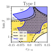
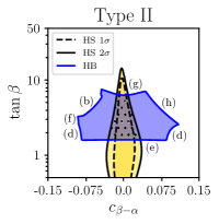
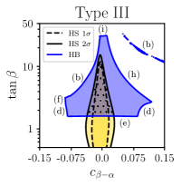
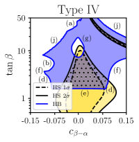
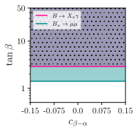
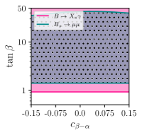
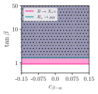
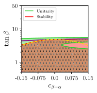
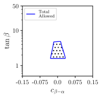
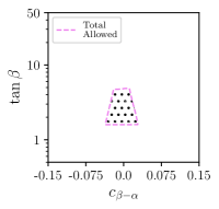
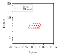
Figure 1: (A) Allowed regions from the restrictions on the parameter space in benchmark scenario 1 in the $c_{\beta-\alpha}$–$\tan\beta$ plane with $m=550\,\,\mathrm{GeV}$ and $m_{12}^{2}=60000\,\,\mathrm{GeV}^{2}$. The results for type I, II, III and IV in the left, second, third and right column, respectively. The upper, second and third row show the restrictions from HiggsBounds/HiggsSignals, the flavor observables and from unitarity/stability, respectively. The fourth row indicates the regions allowed by all constraints in the respective scenario.

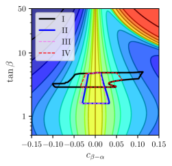
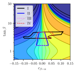
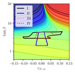
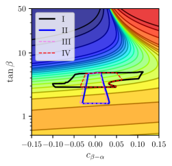
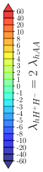
Figure 2: (B) Triple Higgs couplings in benchmark scenario 1 in the $c_{\beta-\alpha}$–$\tan\beta$ plane with $m=550\,\,\mathrm{GeV}$ and $m_{12}^{2}=60000\,\,\mathrm{GeV}^{2}$. Shown are $\kappa_{\lambda}:=\lambda_{hhh}/\lambda_{\mathrm{SM}}$ (upper left), $\lambda_{hhH}$ (upper right), $\lambda_{hHH}$ (lower left) and $\lambda_{hH^{+}H^{-}}=2\lambda_{hAA}$ (lower right). Indicated by the interior of lines are the allowed regions for type I (solid black), type II (solid blue), type III (dashed pink), type IV (dashed red).

We start our comparison in Fig. 2(A) with benchmark scenario 1, i.e. the $c_{\beta-\alpha}-\tan\beta$ plane with $m=550\,\,\mathrm{GeV}$ and $m_{12}^{2}=60000\,\,\mathrm{GeV}^{2}$. The largest differences between the four 2HDM types can be observed in the first row, where we show the restrictions from the LHC data based on the BSM Higgs-boson searches, obtained via HiggsBounds, and on the Higgs-boson rate measurements, obtained via HiggsSignals. Concerning the latter, very roughly speaking, one observes that type I has the “largest allowed” parameter space, and type II resembles type III. Both can be explained by the couplings of the various Higgs bosons to fermions as specified in Tab. 2 as follows. Overall, it can be observed that the parameter space is strongly constrained for $c_{\beta-\alpha}$ to be close to the alignment limit, such that $h$ behaves sufficiently SM-like. In particular, the $2\sigma$ allowed regions for the Yukawa type II and III (2nd and 3rd column) are substantially smaller compared to type I (left column). This is caused by an enhancement of the coupling of $h$ to $b$-quark (see Tab. 2) in these two types. For type IV the restrictions are caused by the enhanced coupling of the $h$ to $\tau$-leptons (which is also present in type II). As $\tan\beta$ increases the types II, III and IV are forced to be very close to the alignment limit to agree with the experimental data. For type I the constraints are weaker, specially for $\tan\beta>3$, where we can accommodate inside the $2\sigma$ region values for $c_{\beta-\alpha}$ between -0.35 and 0.25 when $\tan\beta\sim 6$. For very large values of $\tan\beta$ the restrictions in type I depend strongly on the chosen value of $m_{12}^{2}$, as has been discussed in Ref. [8]. In this benchmark scenario, having a fixed value of $m_{12}^{2}$, (even) in the alignment limit there is an upper limit on $\tan\beta$. This is caused by the charged Higgs contribution to $\Gamma(h\to\gamma\gamma)$. The $hH^{+}H^{-}$ coupling has a contribution that scales with $m_{12}^{2}\,\tan\beta$, such that for fixed $m_{12}^{2}$ extremely large loop contributions and thus extremely large values of $\text{BR}(h\to\gamma\gamma)$ are reached, which are in disagreement with the LHC measurements. On the other hand, in all four types the region allowed by Higgs-boson rate measurements extends to very large values of $\tan\beta$ for $c_{\beta-\alpha}=0$ and $m_{12}^{2}=0$. It is interesting to observe that in the type IV analysis a new allowed branch appears in the upper right part of the plot which corresponds to $\xi_{h}^{d}=-\xi_{h}^{l}=1$, known as the wrong sign Yukawa region. The explicit expression for $\tan\beta$ in this limit, only valid if $c_{\beta-\alpha}>0$, is given by

$$\tan\beta=\frac{1+s_{\beta-\alpha}}{c_{\beta-\alpha}}=\frac{c_{\beta-\alpha}}{1-s_{\beta-\alpha}}.$$ (13)

We now turn to the regions allowed by BSM Higgs-boson searches, shown in blue. The various exclusion bounds are directly related to the Higgs-boson couplings in the respective Yukawa type, as summarized in Tab. 2. The coupling of the heavy Higgs bosons to top-quarks in all four types become large for small $\tan\beta$. Consequently, all four types possess a lower limit for $\tan\beta\sim 1.5$ (with the value of $m_{H^{\pm}}=550\,\,\mathrm{GeV}$ fixed) from the charged Higgs-boson searches, channel (e). For slightly larger $\tan\beta$ and the largest allowed $c_{\beta-\alpha}$ values, the search for $H\to VV$ (channel (d)) becomes relevant, which is then superseded by the channel (f) $gg\to A\to Zh$. However, depending on the type, other channels take over for larger $\tan\beta$. First the channels (c) and (b), via the decay $H\to hh$, become important. Most relevant, however, is the search for $b\bar{b}\to H/A\to\tau\tau$, which becomes important for larger $\tan\beta$ in type II, where the production and decay both scale with $\tan\beta$. Also for type IV this channel becomes important, but only for intermediate $\tan\beta$, since the production channel here scales with $1/\tan\beta$, and only an “island” is excluded by channel (g). In type I, which can extend to larger $\tan\beta$ values than the others, a different channel becomes relevant, $h\to\gamma\gamma$ (a), see the discussion on the Higgs signal rates above. In types II and III for larger $\tan\beta$ and larger positive $c_{\beta-\alpha}$ also the channel (h), $h\to ZZ\to llll$ restricts the allowed parameter space. In type III at very large $\tan\beta$ the channel (i), $H\to\gamma\gamma$ becomes important due to an enhanced $HH^{+}H^{-}$ coupling. Finally, in type IV the channel (j), $h\to\tau\tau$ restricts the allowed parameter space due to the enhanced Higgs coupling to leptons in this Yukawa type.

The restrictions from flavor physics are discussed in the second row of Fig. 2(A). Again type II and type III strongly resemble each other, and type I is very similar to type IV. In general, all the four types of the 2HDM exhibit an excluded area at low $\tan\beta$ values, $\tan\beta\;\raisebox{-3.00003pt}{$\stackrel{{\scriptstyle\displaystyle<}}{{\sim}}$}\;1$. The most constraining observable in this low $\tan\beta$ region is $\text{BR}(B\to X_{s}\gamma)$ in the types I and IV, and $\text{BR}(B_{s}\to\mu\mu)$ in the types II and III. These similarities in the allowed areas of types I and IV, on one hand, and those of types II and III, on the other hand, are due to the dominant loop effects in flavor observables involving the $H^{\pm}$. Its couplings to fermions, given in terms of $\xi_{A}^{u}$ and $\xi_{A}^{d}$, are the same in type I and type IV as well as type II and type III. Furthermore, the case of type II shows a peculiarity at large $\tan\beta$, where a region appears constrained from $B_{s}\to\mu\mu$. This is due to the large contributions from the Higgs-penguin loops that are mediated by the neutral Higgs bosons. These contributions are enhanced maximally in the Yukawa type II due to the involved coupling factors, $\xi_{h,H,A}^{d}$ and $\xi_{h,H,A}^{l}$, which all grow with $\tan\beta$.

The third row of Fig. 2(A) discusses the restrictions from unitarity and stability, which is identical in all four types. Both constraints disallow values of $\tan\beta\gtrsim 5$, since $\lambda_{1}$, $\lambda_{3}$, $\lambda_{4},$ and $\lambda_{5}$, present in Eq. (1), grow with $\tan\beta$, making it complicated to fulfill the theoretical constraints. It can also be seen how Eq. (10), plotted in solid purple, follows the boundary of the allowed region by the stability conditions for $c_{\beta-\alpha}>0$. On the other hand, for negative values of $c_{\beta-\alpha}$, Eq. (11), plotted in dashed yellow, marks this boundary.

The overall allowed parameter regions in the $c_{\beta-\alpha}$-$\tan\beta$ plane in the four 2HDM types is summarized in the last row of Fig. 2(A) as the interior of solid lines (in black, blue, pink and red). In the benchmark scenario 1 the allowed region extends more in $c_{\beta-\alpha}$ for type I, whereas it it extends further down in $\tan\beta$ for types II and III. These allowed regions are now contrasted with the predictions of the various triple Higgs couplings in Fig. 2(B). In the upper left plot the prediction for $\kappa_{\lambda}:=\lambda_{hhh}/\lambda_{\mathrm{SM}}$ is shown. By definition one finds $\kappa_{\lambda}=1$ in the alignment limit, $c_{\beta-\alpha}=0$. Larger deviations from unity are found for larger $|c_{\beta-\alpha}|$, and consequently, type I naturally features larger deviations from the SM. The situation is similar for $\lambda_{hhH}$, as shown in the upper right plot. This coupling goes to zero in the alignment limit, and larger positive (negative) values are found for larger positive (negative) values of $c_{\beta-\alpha}$. Consequently, also for this coupling type I allows for the largest values of $|\lambda_{hhH}|$ (reached for $\tan\beta=3$ in this benchmark plane). The situation is reversed for the trilinear couplings involving two heavy Higgs bosons, as shown in the lower row of Fig. 2, with $\lambda_{hHH}$ on the left and $\lambda_{hH^{+}H^{-}}=2\lambda_{hAA}$ on the right. Larger variations of these couplings are found (in the allowed regions) for a variation of $\tan\beta$ (this pattern changes for $\tan\beta$ values somewhat higher than in the allowed regions). Consequently, the largest values are found in Yukawa types II and III in the lowest allowed $\tan\beta$ region in this benchmark plane. On the other hand, it is interesting to note that the behavior of $\lambda_{hH^{+}H^{-}}$ in the region $\tan\beta\;\raisebox{-3.00003pt}{$\stackrel{{\scriptstyle\displaystyle>}}{{\sim}}$}\;10$ correlates with the parameter space allowed by HiggsSignals in Yukawa type I. As discussed above, this is due to the charged Higgs contribution to $\Gamma(h\to\gamma\gamma)$. Also the other three types would exhibit the same feature, but other constraints already constrain the allowed parameter space to lower $\tan\beta$ and smaller $|c_{\beta-\alpha}|$.

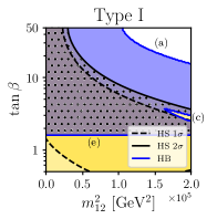
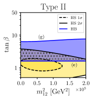
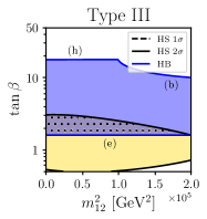
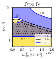
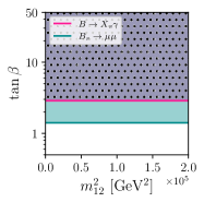
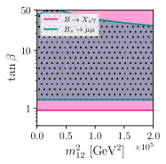
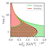
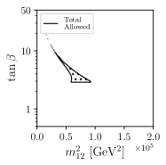
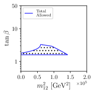
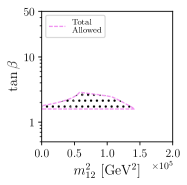
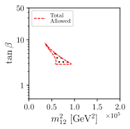
Figure 3: (A) Allowed regions from the restrictions on the parameter space in benchmark scenario 2 in the $m_{12}^{2}$–$\tan\beta$ plane with $m=550\,\,\mathrm{GeV}$ and $c_{\beta-\alpha}=0.02$. The results for type I, II, III and IV in the left, second, third and right column, respectively. The upper, second and third row show the restrictions from HiggsBounds/HiggsSignals, the flavor observables and from unitarity/stability, respectively. The fourth row indicates the regions allowed by all constraints in the respective scenario.

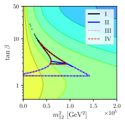
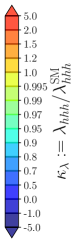
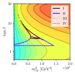
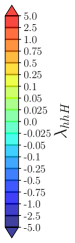
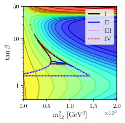
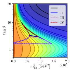
Figure 4: (B) Triple Higgs couplings in benchmark scenario 2 in the $m_{12}^{2}$–$\tan\beta$ plane with $m=550\,\,\mathrm{GeV}$ and $c_{\beta-\alpha}=0.02$. Shown are $\kappa_{\lambda}:=\lambda_{hhh}/\lambda_{\mathrm{SM}}$ (upper left), $\lambda_{hhH}$ (upper right), $\lambda_{hHH}$ (lower left) and $\lambda_{hH^{+}H^{-}}=2\lambda_{hAA}$ (lower right). Indicated by the interior of lines are the allowed regions for type I (solid black), type II (solid blue), type III (dashed pink), type IV (dashed red).

The next set of comparisons of the four 2HDM types, in benchmark scenario 2, in the $m_{12}^{2}$–$\tan\beta$ plane is presented in Fig. 4. The overall mass scale is fixed to $m=550\,\,\mathrm{GeV}$, and $c_{\beta-\alpha}=0.02$, i.e. the decoupling limit is explicitly excluded from this benchmark. As in the first benchmark scenario, the parameter space allowed by the Higgs-boson rate measurements, shown in yellow in the first row of Fig. 4(A) is largest for type I and similar for type II and III. In all four types the lowest $\tan\beta$ values of $\tan\beta\sim 0.5$ are allowed, where in type II and III the largest $m_{12}^{2}$ values shown in combination with very low $\tan\beta$ are excluded, which can be traced back to $h\to\gamma\gamma$. Going to larger $\tan\beta$, the upper limit in type I, and largely also in type IV, is given by the charged Higgs-boson contribution to $\Gamma(h\to\gamma\gamma)$, see the discussion of benchmark 1. In type II and III the upper limit is encountered already for lower $\tan\beta$ values, where the enhancement of the $hb\bar{b}$ coupling becomes stronger in these two types.

Concerning the searches for BSM Higgs bosons, at low $\tan\beta$ the same pattern as in benchmark 1 is observed. The coupling of the heavy Higgs bosons to top-quarks in all four types become large for small $\tan\beta$. Consequently, all four types possess a lower limit for $\tan\beta\sim 1.5$ (and $m_{H^{\pm}}=550\,\,\mathrm{GeV}$) from the search for charged Higgs-boson searches, channel (e). However, the four types differ substantially in their upper $\tan\beta$ limits. In type I all couplings of the heavy Higgs bosons to SM fermions decrease with increasing $\tan\beta$, yielding a large allowed parameter space. The limit then comes from the too large rate in $\text{BR}(h\to\gamma\gamma)$, channel (a). For intermediate $\tan\beta$ and large $m_{12}^{2}$ also the channel (c), $H\to hh$, plays a minor role. The situation is completely different in type II, where $\tan\beta\;\raisebox{-3.00003pt}{$\stackrel{{\scriptstyle\displaystyle>}}{{\sim}}$}\;6$ is excluded from the “classical” search channel $H/A\to\tau\tau$ for this Yukawa type. In type III the situation is again different. For smaller $m_{12}^{2}$ at $\tan\beta\sim 19$ the channel (h), $h\to ZZ\to llll$, becomes important. For these large values of $\tan\beta$ the $hb\bar{b}$ coupling is reduced substantially in type III and, becomes 0 for $\xi_{h}^{d}(\mbox{type III})=s_{\beta-\alpha}-c_{\beta-\alpha}\tan\beta=0$, see Tab. 2. For the chosen value of $c_{\beta-\alpha}=0.02$ this is reached for $\tan\beta\sim 50$. Thus, an increase in $\tan\beta$ yields a decrease of $\Gamma(h\to b\bar{b})$ and correspondingly an increase of $\text{BR}(h\to ZZ\to llll)$, where the experimental bound is reached for $\tan\beta\sim 19$. Going to larger $m_{12}^{2}$ the $H\to hh$ channel (b) takes over. Type IV, because of its Yukawa structure, is restricted at high $\tan\beta$ from $\text{BR}(h\to\gamma\gamma)$, channel (a). However, for small $m_{12}^{2}$, as in benchmark 1, for intermediate $\tan\beta$ values the $H/A\to\tau\tau$ channel becomes strong, where the same interplay as described for benchmark 1 takes place. Consequently, also in benchmark 2 type IV exhibits a “hole” in the allowed parameter space at $\tan\beta\sim 10$. Overall, the lower limits on $\tan\beta$ are set by the charged Higgs-boson searches, which are effectively the same in the four types. On the other hand, the upper limits are given by the Higgs-boson rate measurements, resulting in higher $\tan\beta$ limits in type I and IV, and in quite low limits in type II and III.

The restrictions from flavor physics are discussed in the second row of Fig. 4(A). Again type II and type III strongly resemble each other, and type I is very similar to type IV in the low $\tan\beta$ region, again because the coupling of $H^{\pm}$ to quarks is identical in both cases. For types I and IV, $B\to X_{s}\gamma$ disallows $\tan\beta<3$, whereas for types II and III $B_{s}\to\mu\mu$ is the most constraining observable setting the limit on $\tan\beta\;\raisebox{-3.00003pt}{$\stackrel{{\scriptstyle\displaystyle>}}{{\sim}}$}\;1$. In addition, for type II we see again a disallowed region for large $\tan\beta$ and $m_{12}^{2}$, originating from the effect of the Higgs mediated penguin diagrams in $B_{s}\to\mu\mu$.

The third row of Fig. 4(A) shows the restrictions from unitarity and stability, which are identical in all four types. The largest allowed range for $m_{12}^{2}$ occurs at $\tan\beta\sim 1$, where this parameter can reach values from 0 up to $1.5\times 10^{5}\,\,\mathrm{GeV}^{2}$. For larger values of $\tan\beta$ the region allowed by the unitarity constraints narrows drastically, closing in to Eq. (10) and Eq. (11), plotted in solid purple and dashed yellow respectively. Notice that these two equations provide contour lines in this plane that are at the boundaries of the allowed region by the stability constraints which is also quite narrow at large $\tan\beta$, as can be seen in this figure. If a value for $c_{\beta-\alpha}$ further from the alignment limit was chosen, the narrow region allowed by unitarity shrinks even further and would separate from the allowed region by the stability conditions. In this case, only Eq. (10) will enter in the extremely narrow allowed region by unitarity. Furthermore, Eq. (11) is very close to upper bounds to $m_{12}^{2}$ set by the theoretical constraints for all $\tan\beta$ values. Negative values of $m_{12}^{2}$ are disallowed by the condition that requires the minimum of the potential to be a global minimum.

The overall allowed parameter regions in the $m_{12}^{2}$-$\tan\beta$ plane in benchmark 2 in the four 2HDM types are summarized in the last row of Fig. 4(A). According to our discussion, the regions are similar for type I and IV, as well as for type II and III. In Yukawa types I and IV the regions extend for intermediate $m_{12}^{2}$ from $\tan\beta\sim 3$ to $\tan\beta\sim 10$. Conversely, in type II and III the allowed regions extend from $m_{12}^{2}=0$ to $m_{12}^{2}\sim 150000\,\,\mathrm{GeV}^{2}$ and from $\tan\beta\sim 1.7$ to $\tan\beta\;\raisebox{-3.00003pt}{$\stackrel{{\scriptstyle\displaystyle<}}{{\sim}}$}\;3.5$. This complementarity results in equally complementary results for the tripe Higgs couplings, shown in Fig. 4(B). For $\kappa_{\lambda}$ only a value $\neq 1$ is allowed in types I and IV, although the difference never exceeds 1%. In types II and III, reaching to small $m_{12}^{2}$, also $\kappa_{\lambda}=1$ is almost reached. However, due to the choice $c_{\beta-\alpha}=0.02$, i.e. very close to the decoupling limit, $\kappa_{\lambda}$ is bound to be close to unity. Correspondingly, for $\lambda_{hhH}$ only relatively small values are found. In type I and IV values between 0.1 and 0.25 are found. In type II and III, which allow to go to small $m_{12}^{2}$ and lower $\tan\beta$ values, also smaller $\lambda_{hhH}$ are realized, which can become even negative. Larger values of triple Higgs couplings are possible for $\lambda_{hHH}$, $\lambda_{hAA}$ and $\lambda_{hH^{+}H^{-}}$. However, the overall structure remains as for the other triple Higgs couplings. The contours of the allowed regions for type I and type IV somewhat follow the iso-contours of the three remaining triple Higgs couplings, while the allowed regions for types II and III show larger allowed ranges for $m_{12}^{2}$ in a lower $\tan\beta$ region. Values of $\sim 2$ and $\sim 4$ are found for $\lambda_{hHH}$ and $\lambda_{hAA}=\lambda_{hH^{+}H^{-}}/2$, respectively, in types I and IV. Values up to $\sim 5$ and $\sim 10$, respectively, are found in types II and III, where the largest values are found for $m_{12}^{2}=0$. As in benchmark 1, it is interesting to note that the $\lambda_{hH^{+}H^{-}}$ coupling for large $\tan\beta$ correlates with the parameter space allowed by HiggsSignals in Yukawa type I and IV (due to the charged Higgs contribution to $\Gamma(h\to\gamma\gamma)$).

We finish our comparison of the four 2HDM Yukawa types with benchmark scenario 3, shown in Fig. 6. In this scenario the input parameters are fixed to $c_{\beta-\alpha}=0.01$ and $\tan\beta=3$, and the comparison is performed in the mass plane $m_{12}^{2}$–$m$. As discussed above, the angles have been chosen to find larger regions in the parameter space in all four types that are in agreement with the constraints. As will become clear, in such a case the masses, contrary to the angles, play a very similar role in the four Yukawa types. As before, we start the discussion with the restrictions coming from the Higgs-boson rate measurements at the LHC. In all four types the allowed region goes from low $m$ and $m_{12}^{2}$ to $m\sim 800\,\,\mathrm{GeV}$ (depending somewhat on the Yukawa type) for the largest analyzed $m_{12}^{2}$ values. The allowed regions from BSM Higgs boson searches exhibit a richer structure for $m\;\raisebox{-3.00003pt}{$\stackrel{{\scriptstyle\displaystyle<}}{{\sim}}$}\;500\,\,\mathrm{GeV}$, but very roughly allow points with $m\;\raisebox{-3.00003pt}{$\stackrel{{\scriptstyle\displaystyle<}}{{\sim}}$}\;350\,\,\mathrm{GeV}$, with the exception of type III, where values down to $m\sim 200\,\,\mathrm{GeV}$ are allowed. This is mainly due to the absence of the $H/A\to\tau\tau$ channel (g) in this Yukawa type. The other relevant channels in all four types are $H\to hh$ (b),(l) and $h\to\gamma\gamma$ (a).

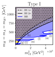
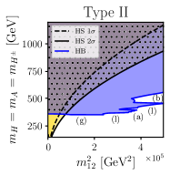
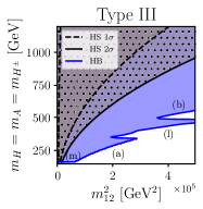
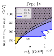
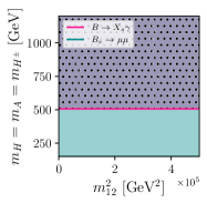
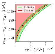
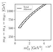
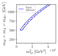
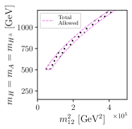
Figure 5: (A) Allowed regions from the restrictions on the parameter space in benchmark scenario 3 in the $m_{12}^{2}$–$m$ plane with $\tan\beta=3$ and $c_{\beta-\alpha}=0.01$. The results for type I, II, III and IV in the left, second, third and right column, respectively. The upper, second and third row show the restrictions from HiggsBounds/HiggsSignals, the flavor observables and from unitarity/stability, respectively. The fourth row indicates the regions allowed by all constraints in the respective scenario.

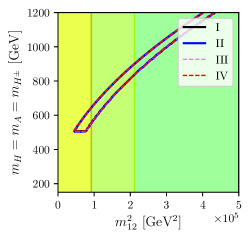
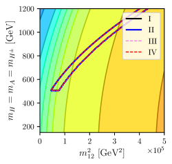
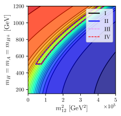
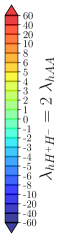
Figure 6: (B) Triple Higgs couplings in benchmark scenario 3 in the $m_{12}^{2}$–$m$ plane with $\tan\beta=3$ and $c_{\beta-\alpha}=0.01$. Shown are $\kappa_{\lambda}:=\lambda_{hhh}/\lambda_{\mathrm{SM}}$ (upper left), $\lambda_{hhH}$ (upper right), $\lambda_{hHH}$ (lower left) and $\lambda_{hH^{+}H^{-}}=2\lambda_{hAA}$ (lower right). Indicated by the interior of lines are the allowed regions for type I (solid black), type II (solid blue), type III (dashed pink), type IV (dashed red).

The restrictions from flavor physics are discussed in the second row of Fig. 6(A). All four types are very similar to each other. For the chosen value of $\tan\beta$, the $\text{BR}(B\to X_{s}\gamma)$ bound on $m\lesssim 500\,\,\mathrm{GeV}$ occurs for the same value of the common heavy Higgs mass, even though the couplings of the heavy Higgs bosons are different in types I and IV as compared to types II and III. On the other hand, the value chosen for $\tan\beta$ makes $\text{BR}(B_{s}\to\mu\mu)$ save for all four types in the whole plane.

The third row of Fig. 6(A) shows the restrictions from unitarity and stability, which by definition are identical in all four types. The unitarity constraints only allow a narrow region with nearly constant width around Eq. (10) and Eq. (11). The stability constraint further reduces the width of the allowed strip where the lower border is then given by Eq. (10) and Eq. (11).

Since we have a small value for $c_{\beta-\alpha}$, both equations are very close. This narrow corridor goes from very low values of $m$ and $m_{12}^{2}$ and it goes to very large values of these parameters, even outside the figure limits on this plane. This plot demonstrates that for values of $\tan\beta$ not much larger than 1, if $m$ increases, $m_{12}^{2}$ can not be arbitrary but it must increase accordingly to satisfy the unitarity and the stability requirements of the theory.

It is in fact the unitarity/stability constraints that restrict the parameter space most. Since this is identical in all four types, and also the other restrictions turn out to be very similar for $c_{\beta-\alpha}$ and $\tan\beta$ fixed to moderate values, the overall allowed parameter space is effectively identical in types I, II, III and IV, as can can be seen in the fourth row of Fig. 6(A). It should be noted that the final allowed narrow corridors in these plots all end at approximately $m=m_{H^{\pm}}=m_{A}=m_{H}=500\,\,\mathrm{GeV}$, where this lower limit on the heavy Higgs boson masses arises from the flavor constraints on $m_{H^{\pm}}$.

The possible values of the triple Higgs couplings in this benchmark plane 3 can be seen in Fig. 6(B). Since $c_{\beta-\alpha}=0.01$ is very close to the alignment limit, $\kappa_{\lambda}\sim 1$ is reached in the four Yukawa types, where the largest deviation of up to $\sim 2\%$ are reached for the largest $m_{12}^{2}$ values. For $\lambda_{hhH}$ values between $\sim 0.025$ and $\sim 0.35$ are found. Similarly, the values reached for $\lambda_{hHH}$ and $\lambda_{hAA}=\lambda_{hH^{+}H^{-}}/2$ do not exceed $\sim 2$, where the allowed region follows the iso-contour lines of these triple Higgs couplings.

4 Analysis of the triple Higgs couplings

In this section we analyze numerically which intervals (or extreme values) of the various triple Higgs couplings are still allowed, taking into account all experimental and theoretical constraints as discussed in Sect. 2.2. In the case of $\lambda_{hhh}$ this is relevant to judge correctly which collider option may be needed to perform a precise experimental determination. For the triple Higgs couplings involving one or two heavy Higgs bosons the analysis will indicate in which processes large effects, e.g. possibly enhanced production cross sections, can be expected due to large triple Higgs couplings (following the strategies discussed in Refs. [10, 11, 12]).

The evaluation has been performed in all four 2HDM types, focusing first on the “simplest” scenario C with fully degenerate heavy Higgs-boson masses $m$. In the final part of this section, showing the complete picture, we also discuss the alternative scenario A with non fully degenerate masses, namely, assuming $m_{H^{\pm}}=m_{A}$ and $m_{H}$ as independent and generically different mass parameters.

The results for scenario C in the following three subsections will be shown in different benchmark planes, which are chosen in each scenario individually. In some benchmark planes the particular values of the other parameters are chosen such as to maximize the deviations of $\lambda_{hhh}$ from it SM value (the plots below show $\kappa_{\lambda}:=\lambda_{hhh}/\lambda_{\mathrm{SM}}$)). Other benchmark planes are chosen such as to maximize the (absolute) size of the triple Higgs couplings involving one or two heavy Higgs bosons. The plots below show the triple Higgs couplings as defined in Eq. (9).

The present analysis in the 2HDM type I has changed only slightly w.r.t. Ref. [8] and we briefly update the corresponding results in Figs. 7 - 10. Concerning the 2HDM type II, the constraints in particular from the Higgs-boson rate measurements have tightened in a relevant way w.r.t. Ref. [8], affecting in particular the allowed ranges for $c_{\beta-\alpha}$. Furthermore, only one scenario with $m\equiv m_{H^{\pm}}=m_{H}=m_{A}$ had been investigated in our previous work Ref. [8]. Consequently, we update our analysis from this previous work analyzing the triple Higgs couplings in several additional planes. The results for the 2HDM types III and IV are new and complete the triple Higgs-boson coupling analysis in the 2HDM. The results in type II and III turned out to be very similar. Consequently, we analyze these two types together, as shown in Figs. 11 - 14. The results for type IV are presented in Figs. 15 - 18.

The figures are organized as follows. The upper rows (the upper row for type I and IV, the upper two for type II and III) summarize the constraints in each benchmark plane: the first, second and third plots correspond to the constraints (with the same color coding) as shown in the first, second and third row of Figs. 2(A), 4(A) and 6(A), i.e. the constraints from Higgs rate measurements and BSM Higgs boson searches, from flavor observables and from unitarity/stability, respectively. The corresponding right plots in Figs. 7 - 18 show the overall allowed region, depicted as dotted areas. The lower rows of Fig. 7 - 18 present the result for the triple Higgs couplings: the first, second, third and fourth plot show the predictions for $\kappa_{\lambda}$, $\lambda_{hhH}$, $\lambda_{hHH}$ and $2\lambda_{hAA}=\lambda_{hH^{+}H^{-}}$, respectively. The overall allowed regions is indicated by a solid black (type I), solid blue (type II), dashed pink (type III) and dashed red line (type IV).

4.1 Triple Higgs couplings in the 2HDM type I

The benchmark planes for the 2HDM type I had been defined in Ref. [8] as:

• $m\equiv m_{H^{\pm}}=m_{H}=m_{A}=1000\,\,\mathrm{GeV}$, $m_{12}^{2}$ fixed via Eq. (10),
  free parameters: $c_{\beta-\alpha}$, $\tan\beta$

• $m\equiv m_{H^{\pm}}=m_{H}=m_{A}=650\,\,\mathrm{GeV}$, $\tan\beta=7.5$,
  free parameters: $c_{\beta-\alpha}$, $m_{12}^{2}$

• $m_{12}^{2}$ fixed via Eq. (10), $\tan\beta=10$,
  free parameters: $c_{\beta-\alpha}$, $m$

• $c_{\beta-\alpha}=0.1$, $m_{12}^{2}$ fixed by Eq. (10),
  free parameters $m\equiv m_{H}=m_{A}=m_{H^{\pm}}$,$\tan\beta$.

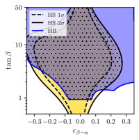
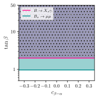
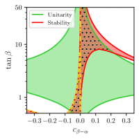
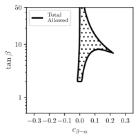
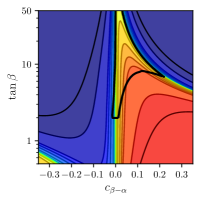
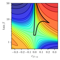
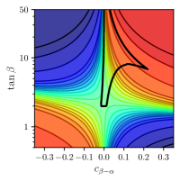
Figure 7: Allowed areas (dotted regions) from the various constraints (upper row) and triple Higgs couplings (lower row) for the benchmark scenario I-1 in the $c_{\beta-\alpha}$–$\tan\beta$ plane with $m_{12}^{2}$ fixed via Eq. (10) and $m=1000\,\,\mathrm{GeV}$.

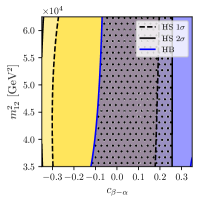
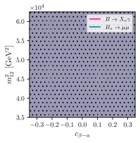
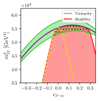
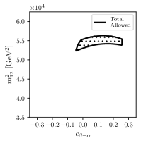
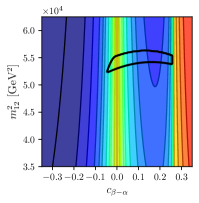
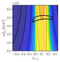
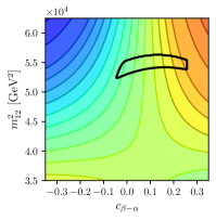
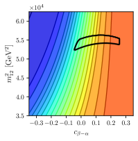
Figure 8: Allowed areas (dotted regions) from the various constraints (upper row) and triple Higgs couplings (lower row) for the benchmark scenario I-2 in the $c_{\beta-\alpha}$–$m_{12}^{2}$ plane with $\tan\beta=7.5$ and $m=650\,\,\mathrm{GeV}$.

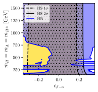
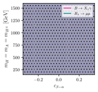
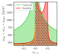
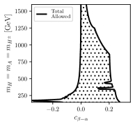
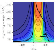
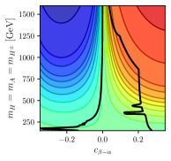
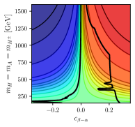
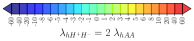
Figure 9: Allowed areas (dotted regions) from the various constraints (upper row) and triple Higgs couplings (lower row) for the benchmark scenario I-3 in the $c_{\beta-\alpha}$–$m$ plane with $\tan\beta=10$ and $m_{12}^{2}$ fixed via Eq. (10).

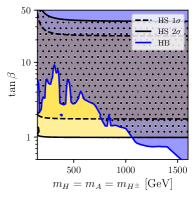
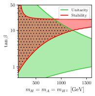
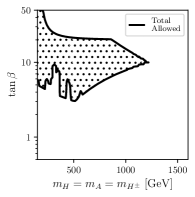
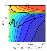
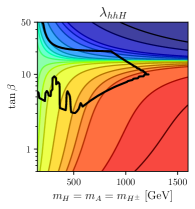
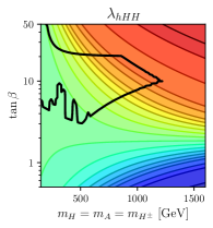
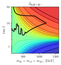
Figure 10: Allowed areas (dotted regions) from the various constraints (upper row) and triple Higgs couplings (lower row) for the benchmark scenario I-4 in the $m$–$\tan\beta$ plane with $c_{\beta-\alpha}=0.2$ and $m_{12}^{2}$ fixed via Eq. (10).

The allowed parameter region in scenario I-1, as shown in Fig. 7, is found mainly for positive $c_{\beta-\alpha}$ with $\tan\beta\geq 2$. The largest allowed $c_{\beta-\alpha}$ values of $\sim 0.2$ are found for $\tan\beta\sim 6$. In the first scenario we found $\kappa_{\lambda}\sim[-0.4,1]$, where the smallest values are reached for these largest $c_{\beta-\alpha}$ points. For $\lambda_{hhH}$ the largest values were found for $c_{\beta-\alpha}\sim 0.08$ and $\tan\beta\sim 7.5$, reaching up to $\lambda_{hhH}\sim 1.2$. The other triple Higgs couplings reach their maximum values around $c_{\beta-\alpha}\sim 0.06$ and $\tan\beta\sim 27$ with $\lambda_{hHH}\approx\lambda_{hAA}=\lambda_{hH^{+}H^{-}}/2\sim 12.5$.

In the second scenario, I-2, shown in Fig. 8, only a very restricted region for $m_{12}^{2}$ is allowed by the constraints, $m_{12}^{2}\sim[52000\,\,\mathrm{GeV}^{2},56000\,\,\mathrm{GeV}^{2}]$. One finds $\kappa_{\lambda}=1$ for $c_{\beta-\alpha}=0$, i.e. in the alignment limit, as required. The same value is also found for $c_{\beta-\alpha}\sim 0.26$ due to cancellations in $\lambda_{hhh}$. Overall, we found $\kappa_{\lambda}\sim[0.5,1.2]$, where the largest values are reached for the largest allowed $c_{\beta-\alpha}\sim 0.28$. The values of $\lambda_{hhH}$ are quite small in this scenario, only reaching up to $\lambda_{hhH}\sim 0.5$. The other triple Higgs couplings reach their maximum values around $c_{\beta-\alpha}\sim 0.26$ and $m_{12}^{2}\sim 55000\,\,\mathrm{GeV}^{2}$ with $\lambda_{hHH}\approx\lambda_{hAA}=\lambda_{hH^{+}H^{-}}/2\sim 6.5$.

The third scenario, I-3, depicted in Fig. 9, exhibits a rather “large” allowed parameter space, where, depending on $m$ we found allowed $c_{\beta-\alpha}$ values between $\sim-0.3$ to $\sim+0.3$. As in the second scenario one finds $\kappa_{\lambda}=1$ not only for $c_{\beta-\alpha}=0$, but also for a second branch with $c_{\beta-\alpha}\geq 0.2$, partially in the “allowed” parameter space. The values that can be reached by $\kappa_{\lambda}$ range from $\kappa_{\lambda}\sim 0.07$ for $c_{\beta-\alpha}\sim 0.1$ and large $m$ close to $1200\,\,\mathrm{GeV}$ to about $\kappa_{\lambda}\sim 1.2$ for the largest allowed $c_{\beta-\alpha}$ values and $m\sim 300\,\,\mathrm{GeV}$. $\lambda_{hhH}$ reaches its maximum value of $\sim 1.7$ for $c_{\beta-\alpha}\sim 0.05$ and $m\sim 1500\,\,\mathrm{GeV}$. The other triple Higgs couplings reach their maximum allowed values around $c_{\beta-\alpha}\sim 0.11$ and $m\sim 1200\,\,\mathrm{GeV}$ with $\lambda_{hHH}\approx\lambda_{hAA}=\lambda_{hH^{+}H^{-}}/2\sim 12.5$.

The final scenario for type I, I-4, is shown in Fig. 10. It is given in the $m$–$\tan\beta$ plane, where for low values of $m$ the largest values of $\tan\beta\sim 50$ are reached. Direct searches and stability/unitarity constraints yield bounds of $m\;\raisebox{-3.00003pt}{$\stackrel{{\scriptstyle\displaystyle<}}{{\sim}}$}\;1200\,\,\mathrm{GeV}$ with $\tan\beta$ ranging between $\sim 3$ and $\sim 20$ (except for the lowest values of $m$. As in the previous planes, we find $\kappa_{\lambda}\sim[0.05,1.05]$, where the largest (smallest) values are reached for the smallest (largest) values of $m$. Similarly, we find $\lambda_{hhH}\sim[-0.5,1.3]$, with the negative values reached for the higher $\tan\beta$ value, and the largest value around the highest allowed values of $m$. As in the other benchmark planes the smallest (largest) values of $\lambda_{hHH}\sim\lambda_{hAA}=\lambda_{hH^{+}H^{-}}/2$ are found for the smallest (largest) values of $m$. Their allowed values are found in the interval $\lambda_{hHH}\sim\lambda_{hAA}=\lambda_{hH^{+}H^{-}}/2\sim[0.2,12]$.

4.2 Triple Higgs couplings in the 2HDM types II and III

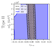
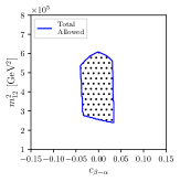
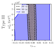
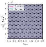
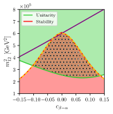
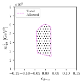
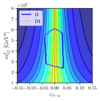
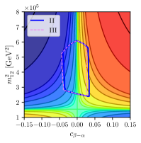
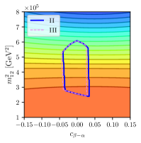
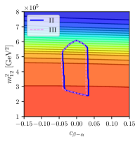
Figure 11: Allowed areas (dotted regions) from the various constraints in type II (upper row) and type III (middle row) and triple Higgs couplings (lower row) for the benchmark scenario II/III-1 in the $c_{\beta-\alpha}$–$m$ plane with $\tan\beta=0.9$ and $m=1100\,\,\mathrm{GeV}$.

The benchmark planes for the 2HDM types II and III are defined as (with the first plane taken over from Ref. [8]):

• $m\equiv m_{H^{\pm}}=m_{H}=m_{A}=1100\,\,\mathrm{GeV}$, $\tan\beta=0.9$,
  free parameters: $c_{\beta-\alpha}$, $m_{12}^{2}$

• $c_{\beta-\alpha}=-0.035$, $\tan\beta=1.2$,
  free parameters: $m_{12}^{2}$, $m\equiv m_{H}=m_{A}=m_{H^{\pm}}$.

• $m\equiv m_{H}=m_{A}=m_{H^{\pm}}=1300\,\,\mathrm{GeV}$, $m_{12}^{2}=700000\,\,\mathrm{GeV}^{2}$,
  free parameters: $c_{\beta-\alpha}$, $\tan\beta$.

• $m\equiv m_{H}=m_{A}=m_{H^{\pm}}=1000\,\,\mathrm{GeV}$, $c_{\beta-\alpha}=-0.035$,
  free parameters: $m_{12}^{2}$, $\tan\beta$.

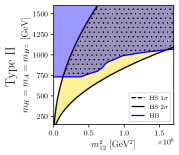
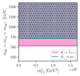
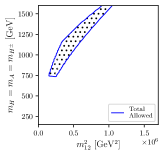
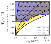
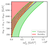
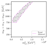
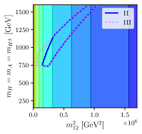
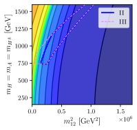
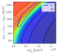
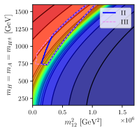
Figure 12: Allowed areas (dotted regions) from the various constraints in type II (upper row) and type III (middle row) and triple Higgs couplings (lower row) for the benchmark scenario II/III-2 in the $m_{12}^{2}$–$m$ plane with $\tan\beta=1.2$ and $c_{\beta-\alpha}=-0.035$.

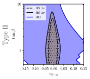
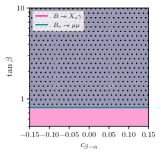
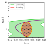
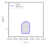
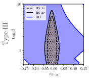
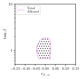
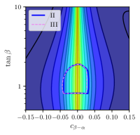
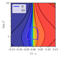
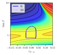
Figure 13: Allowed areas (dotted regions) from the various constraints in type II (upper row) and type III (middle row) and triple Higgs couplings (lower row) for the benchmark scenario II/III-3 in the $c_{\beta-\alpha}$–$\tan\beta$ plane with $m\equiv m_{H}=m_{A}=m_{H^{\pm}}=1300\,\,\mathrm{GeV}$ and $m_{12}^{2}=700000\,\,\mathrm{GeV}^{2}$.

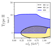
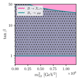
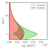
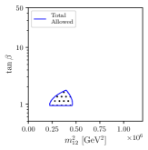
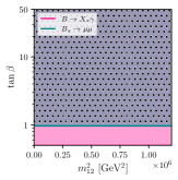
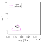
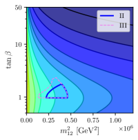
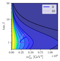
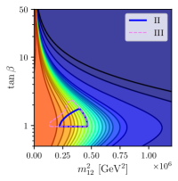
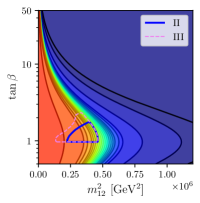
Figure 14: Allowed areas (dotted regions) from the various constraints (upper row) and triple Higgs couplings (lower row) for the benchmark scenario II/III-4 in the $m_{12}^{2}$–$\tan\beta$ plane with $m\equiv m_{H}=m_{A}=m_{H^{\pm}}=1000\,\,\mathrm{GeV}$ and $c_{\beta-\alpha}=-0.035$.

The results for the first scenario II/III-1, shown in Fig. 11, is an update of the same scenario as presented in Ref. [8], but now analyzed for the two Yukawa types II and III. It is shown in the $c_{\beta-\alpha}$–$m_{12}^{2}$ plane with $m=1100\,\,\mathrm{GeV}$ and $\tan\beta=0.9$. The main difference for type II w.r.t. the previous analysis consists in the stronger bounds from the Higgs-boson signal-rate measurements (as included by HiggsSignals). This results in particular in a tighter bound on $c_{\beta-\alpha}$, as can be seen in the upper left plot of Fig. 11, where we find $c_{\beta-\alpha}\sim[-0.04,0.03]$. Flavor constraints allow the whole plane, whereas unitarity/stability selects a nearly triangular region, as can be observed in the upper row, middle-right plot. Together with the tighter bounds from the Higgs-boson rate measurements the dotted area shown in the upper right plot remains allowed in this scenario. Nearly identical results are found in the Yukawa type III, as can be seen in the middle row of Fig. 11. The corresponding allowed regions for the various triple Higgs couplings are shown for both Yukawa types in the lower row of Fig. 11. Since the results are so similar for type II and III here and for Figs. 12 - 14 we only quote a common set of allowed intervals. With the stronger bounds on $c_{\beta-\alpha}$ we find $\kappa_{\lambda}\sim[0.8,1]$, where the largest deviations from unity are found for the largest deviations of $c_{\beta-\alpha}$ from zero, i.e. the alignment limit. Similarly, also $\lambda_{hhH}$ is more restricted in type II than in Ref. [8], $\lambda_{hhH}\sim[-1,0.8]$. The situation is different for the triple Higgs couplings involving two heavy Higgs bosons. These depend only mildly on $c_{\beta-\alpha}$, but strongly on $m_{12}^{2}$. For $\lambda_{hHH}\sim\lambda_{hAA}=\lambda_{hH^{+}H^{-}}/2$ the largest values reached in the allowed area are $\sim 12$, with the largest values found for the smallest $m_{12}^{2}$.

The second scenario for Yukawa types II and III, denoted as II/III-2, is shown in Fig. 12. The overall allowed parameter space, shown as dotted area in the upper and middle right plots is found for $m\sim[750\,\,\mathrm{GeV},1600\,\,\mathrm{GeV}]$ (where the upper limit is the end of our scan range) and $m_{12}^{2}\sim[1.5(0.5)\times 10^{5}\,\,\mathrm{GeV}^{2},10^{6}\,\,\mathrm{GeV}^{2}]$ in type II (III) (where the upper limit is given by the upper limit on $m$). It should be noted that in this scenario the lowest allowed value of $m\sim 750\,\,\mathrm{GeV}$ is set mainly by the flavor constraints on $m_{H^{\pm}}$. The values of $\kappa_{\lambda}$ in this scenario are all smaller than 1, where the smallest value of $\kappa_{\lambda}\sim 0.67$ are found for the largest $m$ and $m_{12}^{2}$ region. $\lambda_{hhH}$ is found to be negative, with the smallest values $\lambda_{hhH}\sim-1.7$ again for the large $m$, $m_{12}^{2}$ region. The largest values of $\lambda_{hHH}$ and $\lambda_{hH^{+}H^{-}}=2\lambda_{hAA}$ are found for the largest values of $m$ and $m_{12}^{2}$ that are reached in the upper right corner of the allowed region, reaching values of $\sim 12$ and $\sim 24$, respectively.

The third scenario of Yukawa types II and III, denoted as II/III-3, is presented in Fig. 13 in the $c_{\beta-\alpha}$–$\tan\beta$ plane. The overall allowed parameter space is given as a combination of all types of constraints and found for $c_{\beta-\alpha}\sim[-0.04,0.03]$ and $\tan\beta\sim[0.7,1.8]$. The deviations in $\lambda_{hhh}$ from the SM value in this scenario are relatively small, $\kappa_{\lambda}\sim[0.66,1]$, where the smallest values are found for the lowest allowed $c_{\beta-\alpha}$. The values $\lambda_{hhH}$ range in $\lambda_{hhH}\sim[-1.4,0.9]$, depending mainly on $c_{\beta-\alpha}$. The values of the triple Higgs couplings involving two heavy Higgs bosons, on the other hand, depends mainly on $\tan\beta$ with the largest values, $\lambda_{hHH}\sim\lambda_{hAA}=\lambda_{hH^{+}H^{-}}/2\sim 5$, are found around $\tan\beta\sim 1$. The smallest values of $\sim 0.1$ are reached at $\tan\beta\sim 1.8$.

The final scenario chosen for Yukawa types II and III, denoted as II-III-4, is shown in Fig. 14 in the $m_{12}^{2}$–$\tan\beta$ plane. The strongest constraints, particularly in $m_{12}^{2}$ are given by a combination of the unitarity/stability limits and the Higgs-boson rate measurements, where the latter yields a reduction of the allowed parameter space in type II w.r.t. type III. Consequently, we will quote different (particularly upper) limits for the tripe Higgs couplings for the two Yukawa types in this scenario. We find for type II (III) $m_{12}^{2}\sim[2.2(1.3)\times 10^{5}\,\,\mathrm{GeV}^{2},4.6\times 10^{5}\,\,\mathrm{GeV}^{2}]$. The lower $\tan\beta$ limit of $\tan\beta\;\raisebox{-3.00003pt}{$\stackrel{{\scriptstyle\displaystyle>}}{{\sim}}$}\;0.95$ is due to the BSM Higgs searches, where the charged Higgs-boson searches yield the exclusion. The dependences of all triple Higgs couplings on the two free parameters are similar in this plane. The smallest (largest) values are found for the largest (smallest) values of $m_{12}^{2}$. The ranges found in this scenario are $\kappa_{\lambda}\sim[0.85,0.93]$, $\lambda_{hhH}\sim[-0.79,-0.22]$ and $\lambda_{hHH}\sim\lambda_{hAA}=\lambda_{hH^{+}H^{-}}/2\sim[1.1,9.2]$ for type II and $\kappa_{\lambda}\sim[0.85,0.96]$, $\lambda_{hhH}\sim[-0.8,-0.01]$ and $\lambda_{hHH}\sim\lambda_{hAA}=\lambda_{hH^{+}H^{-}}/2\sim[1.0,12.2]$ for type III.

4.3 Triple Higgs couplings in the 2HDM type IV

We finish our overview of the four Yukawa types of the 2HDM with three benchmark planes in type IV, which are defined as:

• $m\equiv m_{H}=m_{A}=m_{H^{\pm}}=1300\,\,\mathrm{GeV}$, $c_{\beta-\alpha}=-0.02$,
  free parameters: $m_{12}^{2}$, $\tan\beta$

• $m\equiv m_{H}=m_{A}=m_{H^{\pm}}=1300\,\,\mathrm{GeV}$, $m_{12}^{2}$ fixed by Eq. (11),
  free parameters: $c_{\beta-\alpha}$, $\tan\beta$

• $c_{\beta-\alpha}=0.02$, $m_{12}^{2}$ fixed by Eq. (10),
  free parameters $m\equiv m_{H}=m_{A}=m_{H^{\pm}}$,$\tan\beta$,

• $m_{12}^{2}$ fixed by Eq. (10), $\tan\beta$ fixed via Eq. (13) (wrong sign Yukawa limit),
  free parameters: $c_{\beta-\alpha}$, $m\equiv m_{H}=m_{A}=m_{H^{\pm}}$

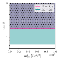
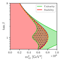
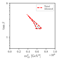
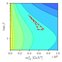
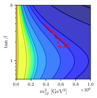
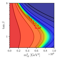
Figure 15: Allowed areas (dotted regions) from the various constraints (upper row) and triple Higgs couplings (lower row) for the benchmark scenario IV-1 in the $m_{12}^{2}$–$\tan\beta$ plane with $m\equiv m_{H}=m_{A}=m_{H^{\pm}}=1300\,\,\mathrm{GeV}$ and $c_{\beta-\alpha}=-0.02$.

The first scenario of type IV, denoted as IV-1, is presented in Fig. 15 in the $m_{12}^{2}$–$\tan\beta$ plane with $m=1300\,\,\mathrm{GeV}$ and $c_{\beta-\alpha}=-0.02$. The lower bound on $\tan\beta$ is given by $\text{BR}(B\to X_{s}\gamma)$ at around $\tan\beta\sim 1.7$. The unitarity/stability constraints then restrict the allowed area to a triangular shape reaching up to $\tan\beta\sim 4$. The variations of $\kappa_{\lambda}$ and $\lambda_{hhH}$ are very small in this small allowed parameter space, with values of $\kappa_{\lambda}\sim 0.92$ and $\lambda_{hhH}\sim-0.7$. The largest values of the other triple Higgs couplings are found for the lowest $\tan\beta$ and at the same time smallest $m_{12}^{2}$. They are given by $\lambda_{hHH}\sim\lambda_{hAA}=\lambda_{hH^{+}H^{-}}/2\sim 6$.

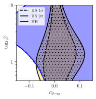
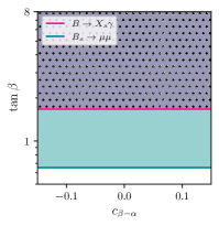
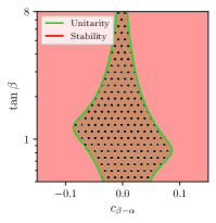
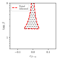
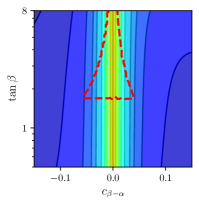
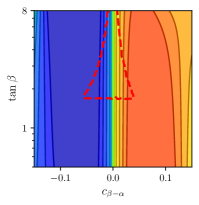
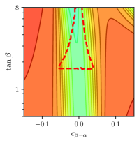
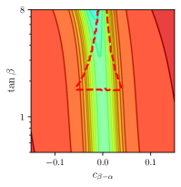
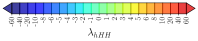
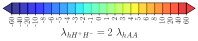
Figure 16: Allowed areas (dotted regions) from the various constraints (upper row) and triple Higgs couplings (lower row) for the benchmark scenario IV-2 in the $c_{\beta-\alpha}$–$\tan\beta$ plane with $m\equiv m_{H}=m_{A}=m_{H^{\pm}}=1300\,\,\mathrm{GeV}$ and $m_{12}^{2}$ fixed by Eq. (11).

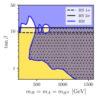
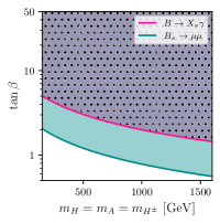
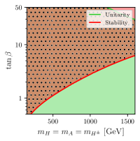
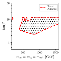
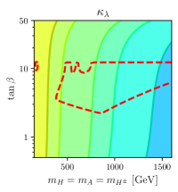
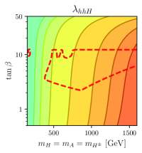
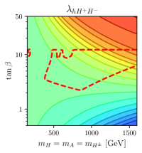
Figure 17: Allowed areas (dotted regions) from the various constraints (upper row) and triple Higgs couplings (lower row) for the benchmark scenario IV-3 in the $m\equiv m_{H}=m_{A}=m_{H^{\pm}}$–$\tan\beta$ plane with $c_{\beta-\alpha}=0.02$ and $m_{12}^{2}$ fixed by Eq. (10).

The second scenario, IV-2, is shown in Fig. 16 in the $c_{\beta-\alpha}$–$\tan\beta$ plane with $m=1300\,\,\mathrm{GeV}$ and $m_{12}^{2}$ fixed by Eq. (11). $\tan\beta$ is restricted by $\text{BR}(B\to X_{s}\gamma)$ to $\tan\beta\;\raisebox{-3.00003pt}{$\stackrel{{\scriptstyle\displaystyle>}}{{\sim}}$}\;1.7$. The remaining parameter space is constrained by unitarity/stability, going up to $\tan\beta=8$, where the scan range ends. $c_{\beta-\alpha}$ is found in the interval $[-0.05,0.04]$, reached for the smallest allowed $\tan\beta$. $\kappa_{\lambda}=1$ is found for $c_{\beta-\alpha}=0$ in the alignment limit, going down to $\kappa_{\lambda}\sim 0.5$ for the smallest allowed $c_{\beta-\alpha}$. $\lambda_{hhH}\sim[-1.59,1.26]$ is found going from the smallest to the largest allowed $c_{\beta-\alpha}$ values. The other three triple Higgs couplings take values around $0$ for $c_{\beta-\alpha}\sim 0$ and large $\tan\beta$. They reach their largest value of $\lambda_{hHH}\sim\lambda_{hAA}=\lambda_{hH^{+}H^{-}}/2\sim 6$ at $c_{\beta-\alpha}\sim-0.05$.

The third type IV scenario, IV-3, is shown in Fig. 17 in the $m$–$\tan\beta$ plane with $c_{\beta-\alpha}=0.02$ and $m_{12}^{2}$ fixed by Eq. (10). Upper and lower limits on $\tan\beta$ are given by the Higgs rate measurements at $\tan\beta=10$ and by the stability bound, respectively. Low values of $m$ are excluded by the BSM Higgs-boson searches at the LHC, leaving a range of about $400\,\,\mathrm{GeV}$ to $1600\,\,\mathrm{GeV}$ (where the scan stopped). $\kappa_{\lambda}$ is found in the interval $\kappa_{\lambda}\sim[0.88,1.00]$, with the smallest (largest) values for large (small) $m$, and nearly independent of $\tan\beta$. Also $\lambda_{hhH}$ is nearly independent of $\tan\beta$ in the allowed parameter range, $\lambda_{hhH}\sim[0.01,1.2]$, where now the largest values are found for large $m$. $\lambda_{hHH}\sim\lambda_{hAA}=\lambda_{hH^{+}H^{-}}/2$ is found around 1 for lower values of $m$ and $\tan\beta$, reaching the highest values of $\sim 5$ for the largest allowed $m$ and $\tan\beta\sim 10$.

The last scenario for Yukawa type IV, IV-4, is presented in Fig. 18 in the $c_{\beta-\alpha}$–$m$ plane with $m_{12}^{2}$ fixed by Eq. (10), and $\tan\beta$ is given by Eq. (13), i.e. such that the wrong sign Yukawa limit is reached. The main restrictions for low $m$ are given by the LHC Higgs rate measurements and the BSM Higgs searches, restricting $c_{\beta-\alpha}\sim 0.25$. The upper limit on $m$ is given by the unitarity constraint, yielding $m\;\raisebox{-3.00003pt}{$\stackrel{{\scriptstyle\displaystyle<}}{{\sim}}$}\;850\,\,\mathrm{GeV}$. $\kappa_{\lambda}$ is smaller than 1, but reaching only deviations of $\kappa_{\lambda}\sim 0.97$. $\lambda_{hhH}$ is found in the interval $[-1.2,0.01]$ with the smallest values reached at large $c_{\beta-\alpha}$ and large $m$. The triple Higgs couplings involving two heavy Higgs bosons depend mainly on $m$, reaching their largest values of $\lambda_{hHH}\sim\lambda_{hAA}=\lambda_{hH^{+}H^{-}}/2\sim 12$ at the highest allowed values of $m$ in this scenario, $m\sim 850\,\,\mathrm{GeV}$.

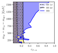
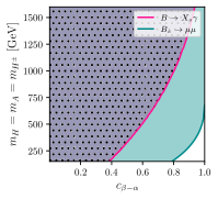
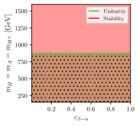
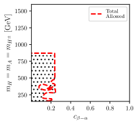
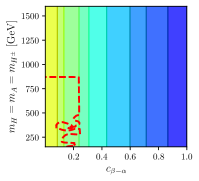
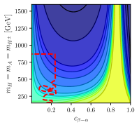
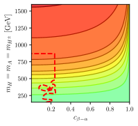
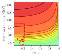
Figure 18: Allowed areas (dotted regions) from the various constraints (upper row) and triple Higgs couplings (lower row) for the benchmark scenario IV-4 in the $c_{\beta-\alpha}$–$m$ plane with $m_{12}^{2}$ fixed by Eq. (10) and $\tan\beta$ fixed via Eq. (13) (wrong sign Yukawa limit).

4.4 Complete picture of allowed triple Higgs couplings

In order to find the overall allowed ranges of the various triple Higgs couplings in the four Yukawa types we have performed a parameter scan. The free parameters were randomly varied in the ranges given in Tab. 3. Following Ref. [8], we here also investigate the possibility of a non-fully degenerate scenario with $m_{A}=m_{H^{\pm}}$ and $m_{H}$ as independent mass parameter (scenario A). For scenario C, with degenerate Higgs bosons masses, $m_{A}=m_{H}=m_{H^{\pm}}$, 10000 valid points were generated. For scenario A, with $m_{A}=m_{H^{\pm}}$ and $m_{H}$ as additional free parameter, 30000 valid points were generated. From now on, we will refer generically to the heavy mass $m_{\rm heavy}$ in this section as the degenerate mass $m=m_{H}=m_{A}=m_{H^{\pm}}$ in scenario C, and to both independent masses $m_{H}$ and $m_{A}=m_{H^{\pm}}$ in scenario A. Naturally, in scenario A slightly larger intervals for the triple Higgs couplings are expected. We consider only these two possibilities, C and A, because in the alternative non-fully degenerate scenarios with $m_{A}=m_{H}$ and $m_{H^{\pm}}$ as independent masses, (named scenario B in Ref. [8]), sizable contributions to the $T$ parameter can appear at two-loop level that may be in conflict with data [77]. Under these assumptions, we always have $2\lambda_{hAA}=\lambda_{hH^{+}H^{-}}$, and in this section we will only refer to $\lambda_{hH^{+}H^{-}}$.

The final allowed intervals for the various triple Higgs couplings are summarized in Tab. 4. One can see that in all four types, $\kappa_{\lambda}$ and $\lambda_{hhH}$ can reach their maximum allowed ranges already in the fully degenerate scenario (with slightly larger possible values of $\kappa_{\lambda}$ in type I). On the other hand, the couplings of the light Higgs with two heavy Higgs bosons, $\lambda_{hHH}$, and $\lambda_{hH^{+}H^{-}}$ can have larger values if some non-degeneracy between $m_{H}$ and $m_{A}=m_{H^{\pm}}$ is allowed (scenario A). In the following we discuss the intervals displayed in Tab. 4, based on our analyses of the benchmark planes in Sects. 4.1 - 4.3.

	Type I	Type II	Type III	Type IV
$m_{\rm heavy}$	[150, 1600]	[450, 1600]	[450, 1600]	[150, 1600]
$\tan\beta$	[1, 50]	[0.5, 50]	[0.5, 50]	[1, 50]
$c_{\beta-\alpha}$	[-0.35, 0.35]	[-0.06, 0.06]	[-0.06, 0.06]	[-0.08, 0.15]
$m_{12}^{2}$	[0, $M_{\rm heavy}^{2}$]	[0, $M_{\rm heavy}^{2}$]	[0, $M_{\rm heavy}^{2}$]	[0, $M_{\rm heavy}^{2}$]

Table 3: Ranges for the input parameters of the 2HDM in our numerical scan. $m_{\rm heavy}$ (given in GeV) refers to $m\equiv m_{H}=m_{A}=m_{H^{\pm}}$ in scenario C and to both independent masses $m_{H}$ and $m_{A}=m_{H^{\pm}}$ in scenario A. The maximum value for $m_{12}^{2}$ taken in our scans is $M_{\rm heavy}^{2}$, where $M_{\rm heavy}$ is the largest of the heavy Higgs boson masses (coinciding with $m_{\rm heavy}$ only in scenario C).

	Type I		Type II
	scenario C	scenario A	scenario C	scenario A
$\kappa_{\lambda}$	[-0.48, 1.23]	[-0.48, 1.28]	[0.62, 1.00]	[0.62, 1.00]
$\lambda_{hhH}$	[-1.69, 1.62]	[-1.69, 1.62]	[-1.80, 1.46]	[-1.80, 1.46]
$\lambda_{hHH}$	[-0.7, 11.5]	[-0.7, 14.5]	[-0.2, 12.3]	[-0.5, 16.2]
$\lambda_{hH^{+}H^{-}}$= 2$\lambda_{hAA}$	[-1.8, 22.6]	[-1.8, 32.8]	[-0.5, 24.6]	[-1.4, 32.7]

	Type III		Type IV†
	scenario C	scenario A	scenario C	scenario A
$\kappa_{\lambda}$	[0.55, 1.00]	[0.55, 1.00]	[0.53, 1.00]	[0.53, 1.01]
$\lambda_{hhH}$	[-1.81, 1.34]	[-1.81, 1.34]	[-1.75, 1.36]	[-1.75, 1.36]
$\lambda_{hHH}$	[-0.3, 12.3]	[-0.2, 15.7]	[-0.6, 8.6]	[-0.6, 9.2]
$\lambda_{hH^{+}H^{-}}$= 2$\lambda_{hAA}$	[-0.7, 24.7]	[-1.3, 32.6]	[-1.2, 16.4]	[-1.7, 32.7]

Table 4: Final allowed ranges for the couplings $\lambda_{hh_{i}h_{j}}$ (for details of the scan, see text). “scenario C” refers to the fully degenerate case with $m=m_{H}=m_{A}=m_{H^{\pm}}$, “scenario A” to the non-fully degenerate case with $m_{A}=m_{H^{\pm}}$ and $m_{H}$ being independent mass parameters (see text). ^†The ranges of type IV do not include the wrong sign Yukawa region.

Focusing first on $\kappa_{\lambda}$, the 2HDM type I is the only type that can accommodate $\kappa_{\lambda}>1$, which can be understood as follows. In type I large values of $\tan\beta$ together with large values of $c_{\beta-\alpha}$ up to $\sim\pm 0.3$ are allowed, as it can be seen in Sects. 3 and 4. Specifically, those $\kappa_{\lambda}>1$ values can be reached in type I when the heavy Higgs boson masses are $m_{\rm heavy}\lesssim 500\,\,\mathrm{GeV}$, $\tan\beta\gtrsim 5$ and $c_{\beta-\alpha}\gtrsim 0.2$. Type I is also found to be the unique one allowing for negative $\kappa_{\lambda}$ values. The minimum allowed value is $\kappa_{\lambda}\sim-0.5$, which is found for $m_{\rm heavy}\sim 800\,\,\mathrm{GeV}$, $\tan\beta\sim 7$ and $c_{\beta-\alpha}$ is at its maximum allowed value around 0.25. In these parts of the parameter space of type I with such large values for $\tan\beta$, close to 10, $m_{12}^{2}$ has to be close the value given by Eq. (10) to satisfy the theoretical constraints. In contrast to type I, in the other three Yukawa types, the lower values of $\kappa_{\lambda}$ that can be reached are around 0.5, corresponding to deviations of around 50% below the SM prediction. They are found for the largest value of the heavy Higgs boson masses $m_{\rm heavy}$ considered in the scan, the lowest allowed value for $\tan\beta$ and the largest allowed value of $|c_{\beta-\alpha}|$, especially for the case of negative $c_{\beta-\alpha}$. In these cases, setting $m_{12}^{2}$ close to the value given by Eq. (11) can help to maximize the deviation on $\kappa_{\lambda}$ from 1 while respecting the theoretical constraints.

Regarding the other types, we see that in type IV the minimum allowed values of $\tan\beta$ around 1 are larger than in types II and III, which are closer to 0.5, due to the $B\to X_{s}\gamma$ constraint, and the effect on $\kappa_{\lambda}$ is expected to be smaller. However, this milder effect at low $\tan\beta$ on $\kappa_{\lambda}$ is compensated by the fact that type IV can accommodate larger values of $|c_{\beta-\alpha}|$ than in types II and III. It is also worth mentioning that the negative deviation from $\kappa_{\lambda}=1$ could be larger with larger heavy Higgs boson masses than those considered in our scans.

In the case of $\lambda_{hhH}$, we find that for all four types the largest values reached for this coupling are roughly $\sim\pm 1.5$. In all four types, the minimum (maximum) value is reached for the mass range close to the maximum scanned value for the heavy Higgs mass $m_{\rm heavy}$, $\tan\beta\sim 1$ and $c_{\beta-\alpha}\sim-0.03$ ($+0.03$). In type I values of $\lambda_{hhH}\sim 1.5$ can also be reached for $\tan\beta\sim 10$. Again, larger values of $m_{\rm heavy}$ could lead to a larger absolute values for this coupling.

Now we turn to the maximum allowed value for $\lambda_{hHH}$. In types I, II and III one can achieve large values up to $\sim 12$ in the fully degenerate scenario C and up to $\sim 16$ in scenario A with non degenerate masses, $m_{H}\neq m_{A}=m_{H^{\pm}}$. However, the region of the parameter space in which those extreme values are achieved are different depending on the 2HDM type. In type I with scenario C, the largest allowed values for $\lambda_{hHH}$ are achieved when all heavy masses are around $1\,\,\mathrm{TeV}$ for rather large values of $c_{\beta-\alpha}\gtrsim 0.1$ and $\tan\beta\gtrsim 7$, with $m_{12}^{2}$ fixed to Eq. (10). In scenario A, this coupling can be enhanced for $m_{H}\sim 1\,\,\mathrm{TeV}>m_{A}=m_{H^{\pm}}$. The situation for types II and III is different, as they can accommodate extreme values for $\lambda_{hHH}$ with $\tan\beta\sim 1$ and being very close to the alignment limit, i.e. near $c_{\beta-\alpha}\sim 0$, for $m_{\rm heavy}\gtrsim 1\,\,\mathrm{TeV}$ in the degenerate scenario and for $m_{H}\gtrsim 1\,\,\mathrm{TeV}$ and $m_{H}>m_{A}=m_{H^{\pm}}$ in the non degenerate scenario. In type IV, $\lambda_{hHH}$ can only acquire values up to $\sim 8$ in the fully degenerate scenario C and up to $\sim 9$ in scenario A. These large values of $\lambda_{hHH}$ close to 10, can only be achieved for very large values of $\tan\beta>10$ and being very close to the alignment limit with $m_{12}^{2}$ set via Eq. (10).

Turning to the other couplings of the light Higgs to two heavy bosons, $\lambda_{hH^{+}H^{-}}=2\lambda_{hAA}$, we find that very large values up to $\sim 16$ and $\sim 32$ are allowed in the four 2HDM types, in the fully degenerate and the non-degenerate scenarios, respectively. In scenario C with degenerate masses, the maximum allowed values for these couplings, $\lambda_{hH^{+}H^{-}}$ and $\lambda_{hAA}$, are found in the same 2HDM parameter space regions, where we have found the maximum value for $\lambda_{hHH}$. However, for the scenario A the situation is different. In all four types, the maximum values are found for $m_{A}=m_{H^{\pm}}\gtrsim 1\,\,\mathrm{TeV}$ and $m_{A}=m_{H^{\pm}}>m_{H}$, for smaller values of $|c_{\beta-\alpha}|$, close to the alignment limit, and for values of $\tan\beta\sim 2$.

For the Yukawa type IV the wrong sign Yukawa limit is still allowed, where $\tan\beta$ is given by Eq. (13). In scenario C within this particular limit some triple Higgs couplings can reach larger values than in the above discussed parameter regions (in which the wrong-sign limit is not reached), as we have seen in Fig. 18. We found that values for $\lambda_{hHH}$ and $\lambda_{hH^{+}H^{-}}$ up to $\sim 12$ and $\sim 24$ are allowed for $c_{\beta-\alpha}\sim 0.25$ and $m_{\rm heavy}\sim 800\,\,\mathrm{GeV}$. We did not consider this limit in scenario A.

Finally, in the last part of this section, we present some concrete examples of benchmark points within the 2HDM, where we find sizeable effects on the triple Higgs couplings. We have focused both on finding sizeable departures from $\kappa_{\lambda}=1$ and on finding large triple couplings of the light Higgs to the heavy Higgs bosons. We summarize our proposed points in Tab. 5. We have provided examples in the four 2HDM-types and, for simplicity, they all have been chosen within the scenario C with degenerate heavy masses, $m=m_{H}=m_{A}=m_{H^{\pm}}$. It should be noted, that type II and III are presented together since they exhibit practically the same results for the selected benchmark points.

Type	$m$	$\tan\beta$	$c_{\beta-\alpha}$	$m_{12}^{2}$	$\kappa_{\lambda}$	$\lambda_{hhH}$	$\lambda_{hHH}$	$\lambda_{hH^{+}H^{-}}=2\lambda_{hAA}$
I	750	5.5	0.25	Eq. (10)	-0.39	0.4	7	12
I	400	12	0.22	12600	1.26	-0.5	3	6
I	650	6	0.2	Eq. (10)	0.13	0.5	4	8
I	1500	1.55	-0.03	Eq. (11)	0.62	-1.7	7	13
I	1500	2	-0.025	820000	0.83	-1.25	3	6
I	600	10	0.2	Eq. (10)	0.99	-0.5	6	12
I	1000	7.5	0.2	Eq. (10)	-0.26	0.07	13	24
II/III	1500	1.0	-0.04	Eq. (11)	0.63	-1.7	7	14
II/III	1000	1.2	-0.035	470000	0.8	-0.8	3	6
II/III	1000	1.0	0.0	140000	1.0	0.0	12	24
II/III	750	0.02	0.02	0	0.99	-0.1	9	19
II/III	550	1.8	0.01	15000	0.99	0.02	5	9
IV	1200	2.0	-0.05	Eq. (11)	0.61	-1.4	4	8
IV	1200	1.8	-0.055	Eq. (11)	0.55	-1.4	5	9
IV	1500	1.55	-0.045	Eq. (11)	0.55	-1.8	8	16
IV	700	2.5	0.09	Eq. (11)	0.65	0.7	2	5
IV	400	3.8	0.06	24000	0.96	1.0	1.3	2.6
IV	550	3.0	0.045	60000	0.95	0.16	2	4
IV	850	Eq. (13)	0.2	Eq. (10)	0.97	-1.05	12	23

Table 5: Example points in the 2HDM types I II, III and IV that shows sizable triple Higgs couplings with at least one light ${\cal CP}$-even Higgs boson, still allowed by the actual data. Bold values are near the extreme value allowed, shown in Tab. 4. All points shown are for scenario C with fully degenerate heavy Higgs bosons. $m=m_{H}=m_{A}=m_{H^{\pm}}$ and $m_{12}^{2}$ are expressed in GeV and GeV² respectively.

As a general remark, each of the points collected in Tab. 5 exhibits the characteristic phenomenological features of the particular type it belongs to, which have already been described above. In particular in type I, several examples with large triple couplings of the light Higgs boson to the heavy Higgs bosons, or/and large deviations from $\kappa_{\lambda}=1$ are shown, with a larger variation in the values of $\tan\beta$, either small and close to 1-2, or moderate and close to 10. This is not the case for the examples found in the other three Yukawa types, where the largest triple couplings correspond always to a rather small value of $\tan\beta\sim 1-2$.

It is interesting to note that values for $\tan\beta>10$ are in principle allowed in all four 2HDM types close to the alignment limit, but they do not lead to sizable triple Higgs couplings. With such large values for $\tan\beta$, the unitarity and stability conditions forces $m_{12}^{2}$ to be close to the value given by Eq. (12). In the fully degenerate scenario, this would lead to the following triple Higgs couplings: $\kappa_{\lambda}=1$, $\lambda_{hhH}=0$ and $\lambda_{hH^{+}H^{-}}=2\lambda_{hHH}=m_{h}^{2}/v^{2}\simeq 0.26$. Some BSM boson searches and $B_{s}\to\mu\mu$ in type II can pose additional constraints, but heavier Higgs bosons would be able elude them. Regarding the values for $c_{\beta-\alpha}$ in this table of points, they basically display a variation in the small window allowed, which is already quite narrow in the types II/III. In type I the largest triple couplings appear at the extremes of the allowed interval $c_{\beta-\alpha}$, i.e.  around 0.2.

The interest of showing these specific benchmark points is that they can provide interesting scenarios to study at the future colliders. In particular, these scenarios could lead to a remarkable BSM phenomenology in the production of two Higgs bosons, since the triple couplings are involved in a relevant way in those processes. The importance of the triple Higgs couplings in the production of the various (neutral) di-Higgs channels, $hh$, $hH$, $HH$ and $AA$ have already been studied for the types I and II and for the future $e^{+}e^{-}$ linear colliders in Refs. [10, 11, 12], with encouraging results. We leave an extension of these collider studies to the complete picture of the four 2HDM Yukawa types for future work.

5 Conclusions

The measurement of the triple Higgs coupling $\lambda_{hhh}$ is one of the important tasks at current and future colliders. Depending on its size relative to the corresponding SM value, higher (or lower) accuracies can be expected at certain collider options. Going beyond $\lambda_{hhh}$, large values of triple Higgs couplings involving BSM Higgs bosons (i.e. Higgs bosons in addition to the one at $\sim 125\,\,\mathrm{GeV}$) can play an important role in the di-Higgs production cross sections at the (HL-)LHC and future $e^{+}e^{-}$ colliders.

In this paper we have investigated triple Higgs couplings in the Two Higgs Doublet Models (2HDM), treating equally all four Yukawa types, focusing on couplings involving at least one light, SM-like Higgs boson. This is an extension of a previous work [8], where we focused on the Yukawa types I and II. We analyze the allowed parameter ranges in the four Yukawa types, taking into account all relevant theoretical and experimental constraints. These comprise from the theory side unitarity and stability conditions. From the experimental side we require agreement with measurements of the SM-like Higgs-boson rates as measured at the LHC, as well as with the direct BSM Higgs-boson searches. Furthermore, we require agreement with flavor observables and the $T$ parameter, representing the most relevant electroweak precision observable. Particularly for type II we find important differences w.r.t. our previous analysis [8] due to updates in the experimental LHC constraints, whereas type I is much less affected.

It is interesting to note that for the unitarity/stability constraints $m_{12}^{2}$ plays an important role: lower (higher) values are favored by the tree-level stability (unitarity) constraint, where $m_{12}^{2}$ controls the size of the intersection region. In order to enlarge the allowed parameter region by these constraints we have employed on several occasions Eqs. (10) and (11). Concerning the Higgs-boson rate measurements at the LHC, $m_{12}^{2}$ enters particularly in $\lambda_{hH^{+}H^{-}}$, and thus in the prediction of $\Gamma(h\to\gamma\gamma)$. Similarly, but less pronounced, it enters via $\lambda_{hH^{+}H^{-}}$ and $\lambda_{HH^{+}H^{-}}$ in the 2HDM prediction for $B_{s}\to\mu^{+}\mu^{-}$ via the $h$ and $H$ Higgs penguins contributions with charged Higgs bosons in the loops.

In a first step of our phenomenological analysis we analyze the four 2HDM in three benchmark planes, chosen identical for the four Yukawa types (and with $m_{H}=m_{A}=m_{H^{\pm}}$). This allows us to directly compare the four types to each other. Overall we find broadly that type I and type IV resemble each other taking all constraints into account, where the allowed parameter range for type I is usually somewhat larger than for type IV. Conversely, also type II and III resemble each other without larger differences in the allowed parameter ranges. These two types are in general more restricted at larger values of $\tan\beta$ due to the Higgs-boson rate measurements and the BSM Higgs-boson searches at the LHC. On the other hand, flavor observables in general lead to stronger restrictions in type I and IV at low $\tan\beta$. The parameter associated to the alignment limit (in which $h$ becomes SM-like), $c_{\beta-\alpha}$ has larger allowed ranges particularly in type I, and somewhat less in type IV. These general differences have a clear impact on the allowed sizes of the various triple Higgs couplings (see below).

In the second step of our analysis we define four benchmark planes individually for each of the four Yukawa types (and again with $m_{H}=m_{A}=m_{H^{\pm}}$), exemplifying where $\lambda_{hhh}$ shows larger deviations from $\lambda_{\mathrm{SM}}$, or where larger values of the other triple Higgs couplings are found. Since type II and III show a very similar phenomenology, we choose the same planes for these two types. Within these benchmark planes we mark the regions allowed by all theoretical and experimental constraints. In this way these planes can be readily used for further phenomenological analyses. As a relevant example we display the triple Higgs couplings involving at least one light Higgs in these planes.

In a third step we determine the overall allowed ranges for the various triple Higgs couplings in the four Yukawa types. These ranges reflect the overall differences found in the first step of our analysis, see above. The ranges were determined in a parameter scan, where besides the “scenario C” with $m_{H}=m_{A}=m_{H^{\pm}}$ we also investigated the case of “scenario A” with $m_{H}\neq m_{A}=m_{H^{\pm}}$ (which naturally results in slightly larger allowed ranges). Concerning $\kappa_{\lambda}:=\lambda_{hhh}/\lambda_{\mathrm{SM}}$, in types II, III and IV allowed intervals of $\kappa_{\lambda}\sim[0.5,1]$ are found. Only in type I values below $\sim 0.5$ and above $\sim 1$ are allowed with the overall interval of $\kappa_{\lambda}\sim[-0.48,1.28]$. The allowed intervals of $\lambda_{hhH}$ are again similar for types II, III and IV with $\lambda_{hhH}\sim[-1.8,1.4]$, whereas for type I one finds $\lambda_{hhH}\sim[-1.7,1.6]$. Concerning the triple Higgs couplings involving two heavy Higgs bosons, the upper and the lower limits roughly follow $\lambda_{hHH}\sim\lambda_{hAA}\sim\lambda_{hH^{+}H^{-}}/2$ in agreement with the symmetry factor in Eq. (9). We roughly find lower allowed limits of $\lambda_{hHH}\sim\lambda_{hAA}\sim-0.8(-0.4)$ in types I, II, IV (type III). For the upper limits, we find in scenario C values up to $\lambda_{hHH}\sim\lambda_{hAA}\sim\lambda_{hH^{+}H^{-}}/2\sim 12-13$ in all Yukawa types. Substantially larger values are found in scenario A as compared to scenario C in all four Yukawa types. For $m_{H}\neq m_{A}=m_{H^{\pm}}$ the upper allowed values in the explored mass range are found at $\lambda_{hHH}\sim\lambda_{hAA}\sim\lambda_{hH^{+}H^{-}}/2\sim 16$. However, it should be kept in mind that an analysis allowing for heavier BSM Higgs bosons could possibly lead to even larger values for the triple Higgs couplings.

These triple Higgs couplings can have a very strong impact on the heavy di-Higgs production at $pp$ and $e^{+}e^{-}$ colliders [10, 11, 12]. As was discussed in these references, large coupling values can possibly facilitate the discovery of heavier 2HDM Higgs bosons. However, here it must be kept in mind that the larger values of triple Higgs couplings involving two heavy Higgs bosons are always realized for larger values of the respective heavy Higgs-boson mass. Therefore, the effects of the large coupling and the heavy mass always go in opposite directions.

To facilitate more detailed analyses, see e.g. Ref. [10], we provide a list of benchmark points that exemplify large deviations from unity in $\kappa_{\lambda}$ or large (positive or negative) values of the other triple Higgs couplings, while being in agreement with the experimental and theoretical constraints. The benchmark points are given for the choice $m\equiv m_{H}=m_{A}=m_{H^{\pm}}$, and they are identical for Yukawa type II and III, reflecting the similarity of these two types. In order to represent the broad phenomenology that the Higgs-boson sector of the 2HDM offers, they vary substantially in their choice of $m$, $\tan\beta$, $c_{\beta-\alpha}$ and how $m_{12}^{2}$ is determined. We leave a more detailed analysis of their phenomenology at the LHC and future $e^{+}e^{-}$ colliders for future work.

Acknowledgements

S.H. thanks K. Radchenko for helpful discussions. The present work has received financial support from the ‘Spanish Agencia Estatal de Investigación” (AEI) and the EU “Fondo Europeo de Desarrollo Regional” (FEDER) through the project FPA2016-78022-P and by the grant IFT Centro de Excelencia Severo Ochoa CEX2020-001007-S funded by MCIN/AEI/10.13039/501100011033. The work of F.A. and S.H. was also supported in part by the grant PID2019-110058GB-C21 funded by MCIN/AEI/10.13039/501100011033 and by ”ERDF A way of making Europe”. F.A. and M.J.H.  also acknowledge financial support from the Spanish “Agencia Estatal de Investigación” (AEI) and the EU “Fondo Europeo de Desarrollo Regional” (FEDER) through the project PID2019-108892RB-I00/AEI/10.13039/501100011033 and from the European Union’s Horizon 2020 research and innovation programme under the Marie Sklodowska-Curie grant agreement No 674896 and No 860881-HIDDeN. The work of F.A. was also supported by the Spanish Ministry of Science and Innovation via an FPU grant with code FPU18/06634.

References

- [1] G. Aad et al. [ATLAS Collaboration], Phys. Lett. B 716 (2012) 1 [arXiv:1207.7214 [hep-ex]].
- [2] S. Chatrchyan et al. [CMS Collaboration], Phys. Lett. B 716 (2012) 30 [arXiv:1207.7235 [hep-ex]].
- [3] G. Aad et al. [ATLAS and CMS Collaborations], JHEP 1608 (2016) 045 [arXiv:1606.02266 [hep-ex]].
- [4] J. F. Gunion, H. E. Haber, G. L. Kane and S. Dawson, Front. Phys. 80 (2000), 1-404, SCIPP-89/13. Erratum: [arXiv:hep-ph/9302272 [hep-ph]].
- [5] M. Aoki, S. Kanemura, K. Tsumura and K. Yagyu, Phys. Rev. D 80, 015017 (2009) [arXiv:0902.4665 [hep-ph]].
- [6] G. C. Branco, P. M. Ferreira, L. Lavoura, M. N. Rebelo, M. Sher and J. P. Silva, Phys. Rept. 516 (2012) 1 [arXiv:1106.0034 [hep-ph]].
- [7] S. L. Glashow and S. Weinberg, Phys. Rev. D 15, 1958 (1977).
- [8] F. Arco, S. Heinemeyer and M. J. Herrero, Eur. Phys. J. C 80 (2020) no.9, 884 [arXiv:2005.10576 [hep-ph]].
- [9] J. Bernon, J. F. Gunion, H. E. Haber, Y. Jiang and S. Kraml, Phys. Rev. D 92 (2015) no.7, 075004 [arXiv:1507.00933 [hep-ph]].
- [10] F. Arco, S. Heinemeyer and M. J. Herrero, Eur. Phys. J. C 81 (2021) no.10, 913 [arXiv:2106.11105 [hep-ph]].
- [11] F. Arco, S. Heinemeyer and M. J. Herrero, [arXiv:2105.06976 [hep-ph]].
- [12] F. Arco, S. Heinemeyer and M. J. Herrero, PoS EPS-HEP2021 (2022), 609 [arXiv:2110.14424 [hep-ph]].
- [13] T. Kon, T. Nagura, T. Ueda and K. Yagyu, Phys. Rev. D 99, no.9, 095027 (2019) [arXiv:1812.09843 [hep-ph]].
- [14] N. Sonmez, JHEP 10 (2018), 083 [arXiv:1806.08963 [hep-ph]].
- [15] J. de Blas, M. Cepeda, J. D’Hondt, R. Ellis, C. Grojean, B. Heinemann, F. Maltoni, A. Nisati, E. Petit, R. Rattazzi and W. Verkerke, JHEP 01 (2020), 139 [arXiv:1905.03764 [hep-ph]].
- [16] B. Di Micco, M. Gouzevitch, J. Mazzitelli, C. Vernieri, J. Alison, K. Androsov, J. Baglio, E. Bagnaschi, S. Banerjee and P. Basler, et al. Rev. Phys. 5 (2020), 100045 [arXiv:1910.00012 [hep-ph]].
- [17] J. Strube [ILC Physics and Detector Study], Nucl. Part. Phys. Proc. 273-275 (2016), 2463-2465
- [18] P. Roloff et al. [CLICdp], Eur. Phys. J. C 80 (2020) no.11, 1010 [arXiv:1901.05897 [hep-ex]].
- [19] G. Bhattacharyya and D. Das, Pramana 87 (2016) no.3, 40 [arXiv:1507.06424 [hep-ph]].
- [20] A. G. Akeroyd, A. Arhrib and E. M. Naimi, Phys. Lett. B 490 (2000) 119 [hep-ph/0006035].
- [21] A. Barroso, P. M. Ferreira, I. P. Ivanov and R. Santos, JHEP 1306 (2013) 045 [arXiv:1303.5098 [hep-ph]].
- [22] P. Bechtle, O. Brein, S. Heinemeyer, G. Weiglein and K. E. Williams, Comput. Phys. Commun. 181 (2010) 138 [arXiv:0811.4169 [hep-ph]].
- [23] P. Bechtle, O. Brein, S. Heinemeyer, G. Weiglein and K. E. Williams, Comput. Phys. Commun. 182 (2011) 2605 [arXiv:1102.1898 [hep-ph]].
- [24] P. Bechtle, O. Brein, S. Heinemeyer, O. Stål, T. Stefaniak, G. Weiglein and K. E. Williams, Eur. Phys. J. C 74 (2014) no.3, 2693 [arXiv:1311.0055 [hep-ph]].
- [25] P. Bechtle, S. Heinemeyer, O. Stål, T. Stefaniak and G. Weiglein, Eur. Phys. J. C 75 (2015) no.9, 421 [arXiv:1507.06706 [hep-ph]].
- [26] P. Bechtle, D. Dercks, S. Heinemeyer, T. Klingl, T. Stefaniak, G. Weiglein and J. Wittbrodt, Eur. Phys. J. C 80 (2020) no.12, 1211 [arXiv:2006.06007 [hep-ph]].
- [27] V. Khachatryan et al. [CMS Collaboration], Eur. Phys. J. C 74 (2014) no.10, 3076 [arXiv:1407.0558 [hep-ex]].
- [28] M. Aaboud et al. [ATLAS Collaboration], JHEP 01 (2019), 030 [arXiv:1804.06174 [hep-ex]].
- [29] G. Aad et al. [ATLAS Collaboration], Phys. Lett. B 800 (2020), 135103 [arXiv:1906.02025 [hep-ex]].
- [30] M. Aaboud et al. [ATLAS Collaboration], Phys. Rev. D 98 (2018) no.5, 052008 [arXiv:1808.02380 [hep-ex]].
- [31] ATLAS Collaboration, ATLAS-CONF-2020-039.
- [32] A. M. Sirunyan et al. [CMS Collaboration], Eur. Phys. J. C 79 (2019) no.7, 564 [arXiv:1903.00941 [hep-ex]].
- [33] G. Aad et al. [ATLAS Collaboration], Phys. Rev. Lett. 125 (2020) no.5, 051801 [arXiv:2002.12223 [hep-ex]].
- [34] S. Chatrchyan et al. [CMS Collaboration], Phys. Rev. D 89 (2014) no.9, 092007 [arXiv:1312.5353 [hep-ex]].
- [35] CMS Collaboration, CMS-PAS-HIG-12-043.
- [36] M. Aaboud et al. [ATLAS Collaboration], Phys. Lett. B 775 (2017), 105-125 [arXiv:1707.04147 [hep-ex]].
- [37] M. Aaboud et al. [ATLAS Collaboration], Phys. Rev. Lett. 121 (2018) no.19, 191801 [erratum: Phys. Rev. Lett. 122 (2019) no.8, 089901] [arXiv:1808.00336 [hep-ex]].
- [38] M. Aaboud et al. [ATLAS Collaboration], JHEP 09 (2018), 139 [arXiv:1807.07915 [hep-ex]].
- [39] P. Bechtle, S. Heinemeyer, O. Stål, T. Stefaniak and G. Weiglein, Eur. Phys. J. C 74 (2014) no.2, 2711 [arXiv:1305.1933 [hep-ph]].
- [40] P. Bechtle, S. Heinemeyer, O. Stål, T. Stefaniak and G. Weiglein, JHEP 1411 (2014) 039 [arXiv:1403.1582 [hep-ph]].
- [41] P. Bechtle, S. Heinemeyer, T. Klingl, T. Stefaniak, G. Weiglein and J. Wittbrodt, Eur. Phys. J. C 81 (2021) no.2, 145 [arXiv:2012.09197 [hep-ph]].
- [42] References for the individual measurements from the LHC and the Tevatron can be found in: https://higgsbounds.hepforge.org/downloads.html .
- [43] F. Mahmoudi, Comput. Phys. Commun. 180 (2009) 1579 [arXiv:0808.3144 [hep-ph]].
- [44] F. Mahmoudi, Comput. Phys. Commun. 180 (2009), 1718-1719.
- [45] X. Q. Li, J. Lu and A. Pich, JHEP 1406 (2014) 022 [arXiv:1404.5865 [hep-ph]].
- [46] X. D. Cheng, Y. D. Yang and X. B. Yuan, Eur. Phys. J. C 76 (2016) no.3, 151 [arXiv:1511.01829 [hep-ph]].
- [47] P. Arnan, D. Becirevic, F. Mescia and O. Sumensari, Eur. Phys. J. C 77 (2017) no.11, 796 [arXiv:1703.03426 [hep-ph]].
- [48] S. Chen et al. [CLEO], Phys. Rev. Lett. 87 (2001), 251807 [arXiv:hep-ex/0108032 [hep-ex]].
- [49] B. Aubert et al. [BaBar], Phys. Rev. D 77, 051103 (2008) [arXiv:0711.4889 [hep-ex]].
- [50] A. Limosani et al. [Belle], Phys. Rev. Lett. 103, 241801 (2009) [arXiv:0907.1384 [hep-ex]].
- [51] J. Lees et al. [BaBar], Phys. Rev. Lett. 109, 191801 (2012) [arXiv:1207.2690 [hep-ex]].
- [52] J. Lees et al. [BaBar], Phys. Rev. D 86, 052012 (2012) [arXiv:1207.2520 [hep-ex]].
- [53] T. Saito et al. [Belle], Phys. Rev. D 91 (2015) no.5, 052004 [arXiv:1411.7198 [hep-ex]].
- [54] T. Aaltonen et al. [CDF Collaboration], Phys. Rev. D 87 (2013) no.7, 072003 [arXiv:1301.7048 [hep-ex]].
- [55] R. Aaij et al. [LHCb Collaboration], Phys. Rev. Lett. 119, no.4, 041802 (2017) [arXiv:1704.07908 [hep-ex]].
- [56] M. Aaboud et al. [ATLAS Collaboration], JHEP 04 (2019), 098 [arXiv:1812.03017 [hep-ex]].
- [57] A. M. Sirunyan et al. [CMS], JHEP 04 (2020), 188 [arXiv:1910.12127 [hep-ex]].
- [58] P. A. Zyla et al. [Particle Data Group], PTEP 2020 (2020) no.8, 083C01
- [59] M. E. Peskin and T. Takeuchi, Phys. Rev. Lett. 65 (1990) 964.
- [60] M. E. Peskin and T. Takeuchi, Phys. Rev. D 46 (1992) 381.
- [61] W. Grimus, L. Lavoura, O. M. Ogreid and P. Osland, J. Phys. G 35 (2008) 075001 [arXiv:0711.4022 [hep-ph]].
- [62] G. Funk, D. O’Neil and R. M. Winters, Int. J. Mod. Phys. A 27 (2012) 1250021 [arXiv:1110.3812 [hep-ph]].
- [63] D. Eriksson, J. Rathsman and O. Stål, Comput. Phys. Commun. 181 (2010) 189 [arXiv:0902.0851 [hep-ph]].
- [64] A. M. Sirunyan et al. [CMS Collaboration], Eur. Phys. J. C 79 (2019) no.5, 421 [arXiv:1809.10733 [hep-ex]].
- [65] G. Aad et al. [ATLAS Collaboration], Phys. Rev. D 101 (2020) no.1, 012002 [arXiv:1909.02845 [hep-ex]].
- [66] F. Kling, S. Su and W. Su, JHEP 06 (2020), 163 [arXiv:2004.04172 [hep-ph]].
- [67] H. Abouabid, A. Arhrib, D. Azevedo, J. E. Falaki, P. M. Ferreira, M. Mühlleitner and R. Santos, [arXiv:2112.12515 [hep-ph]].
- [68] S. Bertolini, Nucl. Phys. B 272 (1986) 77.
- [69] W. Hollik, Z. Phys. C 32 (1986) 291.
- [70] T. Enomoto and R. Watanabe, JHEP 1605 (2016) 002 [arXiv:1511.05066 [hep-ph]].
- [71] O. Atkinson, M. Black, C. Englert, A. Lenz, A. Rusov and J. Wynne, [arXiv:2202.08807 [hep-ph]].
- [72] A. Arbey, F. Mahmoudi, O. Stål and T. Stefaniak, Eur. Phys. J. C 78 (2018) no.3, 182 [arXiv:1706.07414 [hep-ph]].
- [73] J. Haller, A. Hoecker, R. Kogler, K. Mönig, T. Peiffer and J. Stelzer, Eur. Phys. J. C 78 (2018) no.8, 675 [arXiv:1803.01853 [hep-ph]].
- [74] S. Kraml, T. Q. Loc, D. T. Nhung and L. D. Ninh, SciPost Phys. 7 (2019) no.4, 052 [arXiv:1908.03952 [hep-ph]].
- [75] T. Biekötter, S. Heinemeyer, J.M. No, M.O. Olea and G. Weiglein, IFT–UAM/CSIC–22-015.
- [76] H. Bahl, J. Braathen and G. Weiglein, [arXiv:2202.03453 [hep-ph]].
- [77] S. Hessenberger and W. Hollik, Eur. Phys. J. C 77 (2017) no.3, 178 [arXiv:1607.04610 [hep-ph]].