Sample-efficient Iterative Lower Bound Optimization of
Deep Reactive Policies for Planning in Continuous MDPs

Abstract

Recent advances in deep learning have enabled optimization of deep reactive policies (DRPs) for continuous MDP planning by encoding a parametric policy as a deep neural network and exploiting automatic differentiation in an end-to-end model-based gradient descent framework. This approach has proven effective for optimizing DRPs in nonlinear continuous MDPs, but it requires a large number of sampled trajectories to learn effectively and can suffer from high variance in solution quality. In this work, we revisit the overall model-based DRP objective and instead take a minorization-maximization perspective to iteratively optimize the DRP w.r.t. a locally tight lower-bounded objective. This novel formulation of DRP learning as iterative lower bound optimization ($\operatorname{ILBO}$) is particularly appealing because (i) each step is structurally easier to optimize than the overall objective, (ii) it guarantees a monotonically improving objective under certain theoretical conditions, and (iii) it reuses samples between iterations thus lowering sample complexity. Empirical evaluation confirms that $\operatorname{ILBO}$ is significantly more sample-efficient than the state-of-the-art DRP planner and consistently produces better solution quality with lower variance. We additionally demonstrate that $\operatorname{ILBO}$ generalizes well to new problem instances (i.e., different initial states) without requiring retraining.

1 Introduction

In the past decade, deep learning (DL) methods have demonstrated remarkable success in a variety of complex applications in computer vision, natural language, and signal processing (Krizhevsky, Sutskever, and Hinton 2017; Hinton et al. 2012; Bengio, Lecun, and Hinton 2021). More recently, a variety of work has sought to leverage DL tools for planning and policy learning in a large variety of deterministic and stochastic decision-making domains (Wu, Say, and Sanner 2017; Bueno et al. 2019; Wu, Say, and Sanner 2020; Say et al. 2020; Scaroni et al. 2020; Say 2021; Toyer et al. 2020; Garg, Bajpai, and Mausam 2020).

A large amount of this work has focused on learning (deep reactive) policies in discrete planning settings such as exploiting structure in discrete relational planning models (Issakkimuthu, Fern, and Tadepalli 2018) or learning policies for effective transfer and generalized planning over different domain instantiations of these relational models (Groshev et al. 2018; Toyer et al. 2018; Bajpai, Garg, and Mausam 2018; Garg, Bajpai, and Mausam 2019, 2020; Toyer et al. 2020). Other recent work has investigated planning by discrete and mixed integer optimization in learned discrete neural network models of planning domains (Say and Sanner 2018; Say et al. 2020). Further afield, policy learning has been applied for planning in discrete models through the use of policy gradient methods (Buffet and Aberdeen 2009, 2007; Aberdeen 2005), although it is critical to remark that these methods focused on model-free reinforcement learning approaches and do not directly exploit optimization over the known model dynamics that we explore in this work.

There has been considerably less research focus in the challenging area of planning in nonlinear continuous MDP models that we focus on in this paper. However, a recent direction of significant influence on the present work is the use of automatic differentiation in an end-to-end model-based gradient descent framework to leverage recent advances in non-convex optimization from DL. The majority of work in this direction has focused on deterministic continuous planning models — both known (Wu, Say, and Sanner 2017; Scaroni et al. 2020) and learned (Wu, Say, and Sanner 2020; Say 2021). However, in this work we are specifically concerned with learning deep reactive policies (DRPs) for fast decision-making in general continuous state-action MDPs (CSA-MDPs). While there has been work on planning in CSA-MDPs with piecewise linear dynamics via symbolic methods (Zamani, Sanner, and Fang 2012) or mixed integer linear programming (Raghavan et al. 2017), these methods suffer from scalability limitations and do not learn reusable DRPs for general nonlinear dynamics or reward. The state-of-the-art solution for DRP learning in such nonlinear CSA-MDPs is provided by $\operatorname{tfmdp}$ (Bueno et al. 2019), which optimizes DRPs end-to-end by leveraging gradients backpropagated through the model dynamics and policy.

While $\operatorname{tfmdp}$ made significant advances in solving nonlinear CSA-MDPs, it requires a large number of sampled trajectories to learn effectively and can suffer from high variance in solution quality. In this work, we revisit the overall model-based DRP objective and instead take a fundamentally different approach to its optimization. Specifically, we make the following contributions:

First, for CSA-MDPs with stochastic transitions, we develop a lower bound for the planning objective for optimizing parameterized DRPs by using techniques from convex optimization and minorize-maximize (MM) methods (Lange 2016; Hunter and Lange 2004). Exactly optimizing this lower bound is guaranteed to increase the original planning objective monotonically. Second, we show that this lower bound has a particularly convenient structure for sample-efficient optimization. We also develop techniques that allow us to effectively utilize both

recent and past data for learning the value function and optimizing the lower bound. This improves sample efficiency and lowers the variance in solution quality. We show that our method can generalize to new problem instances (i.e., different initial states) without retraining. Empirically, we perform evaluation on three different domains introduced in (Bueno et al. 2019). Results confirm that our method ILBO is significantly more sample-efficient than the state-of-the-art $\operatorname{tfmdp}$ DRP planner and produces better solution quality with lower variance consistently across all the domains and a variety of hyperparameter settings.

2 Problem Formulation

A Markov decision process (MDP) model is defined using the tuple $(S,A,\mathcal{T},r,\gamma)$. An agent can be in one of the states $s_{t}\in S$ at time $t$. It takes an action $a_{t}\in A$, receives a reward $r(s_{t},a_{t})$, and the world transitions stochastically to a new state $s_{t+1}$ with probability $p(s_{t+1}|s_{t},a_{t})\!=\!\mathcal{T}(s_{t},a_{t},s_{t+1})$. We assume that rewards are non-negative. For the infinite-horizon setting, future rewards are discounted using a factor $\gamma<1$; for finite-horizon settings $\gamma=1$. The initial state distribution is denoted by $b_{0}(s)$. We assume continuous, multi-dimensional state and action spaces ($S\subseteq\mathbb{R}^{n}$, $A\subseteq\mathbb{R}^{n}$) and denote this as a continuous state-action MDP (CSA-MDP).

The empirical experiments conducted focus on transition function that can be factored, similar to factored MDPs (Boutilier, Dean, and Hanks 1999). That is, the transition function can be decomposed as: $p(s_{t+1}|s_{t},a_{t})\!=\!\prod_{j=1}^{n}p(s_{t+1}^{j}|s_{t},a_{t})$ where $s_{t+1}^{j}$ is the $j$th component of the state $s_{t+1}$. However, our proposed approach does not require factorization of transition probabilities in general.

Policy: We follow a similar setting as in (Bueno et al. 2019) and optimize a deterministic policy $\mu_{\theta}$. The Markovian policy $\mu_{\theta}(s)$ provides the deterministic action $a\!=\!\mu_{\theta}(s)$ that is to be executed when the agent is in state $s$. The policy $\mu_{\theta}$ is parameterized using $\theta$ (e.g., $\theta$ may represent parameters of a deep neural net).

Objective: The state value function is defined as the expected total reward received by following the policy $\mu$ from the state $s_{t}$ as: $V^{\mu}(s_{t})=\mathbb{E}\Big{[}\sum_{T=t}^{\infty}\gamma^{T-t}r(s_{T},\mu_{\theta}(s_{T}))\Big{|}s_{t})\Big{]}$. For the finite-horizon setting, we only accumulate rewards until a finite-horizon $H$. The agent’s goal is to find the optimal policy $\mu^{\star}$ maximizing the objective $J$ as:

$$J(\mu)=\mathbb{E}_{s_{0}\sim b_{0}}\Big{[}V^{\mu}(s_{0})\Big{]}$$ (1)

where $b_{0}$ is the initial state distribution.

3 The Minorize-Maximize (MM) Framework

Our approach for optimizing DRPs is based on the MM framework; we briefly review it here and refer the reader to Lange (2016) for full details. Assume the goal is to solve the optimization problem $\max_{\mu}J(\mu)$. The MM framework provides an iterative approach where at each step $m=0,1,\ldots$, we construct a function $\hat{J}(\mu;\mu^{m})$ (assume that $\mu^{0}$ is some given starting estimate). The function $\hat{J}(\mu;\mu^{m})$ minorizes the objective $J(\mu)$ at $\mu^{m}$ iff:

$$\hat{J}(\mu;\mu^{m}) \leq J(\mu)\;\forall\mu$$ (2)

$$\hat{J}(\mu^{m};\mu^{m}) =J(\mu^{m})$$ (3)

In the MM framework, we then iteratively optimize the following problem:

$$\mu^{m+1}=\arg\max_{\mu}\hat{J}(\mu;\mu^{m})$$ (4)

The above step is the so-called maximize operation in the MM algorithm. This scheme results in a monotonic increase in the solution quality until convergence (when $\mu^{m}=\mu^{m+1}$), where we note the minorization property ensures

$$J(\mu^{m+1})\geq\hat{J}(\mu^{m+1};\mu^{m})\,.$$ (5)

Given the maximize operation in (4), we also have $\hat{J}(\mu^{m+1};\mu^{m})\geq\hat{J}(\mu^{m};\mu^{m})$. And we know from condition  (3) that $\hat{J}(\mu^{m};\mu^{m})=J(\mu^{m})$. Therefore, $J(\mu^{m+1})\geq J(\mu^{m})$, which shows that the MM algorithm iteratively improves the solution quality until convergence to a local optimum or a saddle point (Lange 2016).

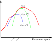
Figure 1: Minorize-Maximize (MM) framework

The geometric intuition behind the MM approach is shown in figure 1. We first construct a lower bound $\hat{J}$ of $J$ at the initial estimate $\mu^{0}$ (or the blue curve $\hat{J}(\mu;\mu^{0})$). Then we maximize $\hat{J}(\mu;\mu^{0})$ to get the next estimate $\mu^{1}$. This step also improves the solution quality as $J(\mu^{1})\geq J(\mu^{0})$. We then keep repeating this process iteratively by constructing a new lower bound at $\mu^{1}$ (in green) and maximizing it to get the next estimate until convergence.

Our goal would be to develop such an MM algorithm for planning in CSA-MDPs. Several algorithms in machine learning are based on the MM framework. The well-known expectation-maximization (EM) algorithm (Dempster, Laird, and Rubin 1977) can be derived from the MM perspective, along with other examples noted in (Hunter and Lange 2004).

In the context of MDPs (and reinforcement learning), several other methods also fall under the umbrella of MM algorithms such as trust region policy optimization (TRPO) (Schulman et al. 2015b). In contrast to the lower bound in TRPO, our derived lower bounds are much simpler, differentiable, and explicitly involve the gradient of the known reward and transition function in the objective, which is desirable for the planning context. The lower bound in (Schulman et al. 2015b) relies on KL divergence based non-differentiable penalty terms, and requires several approximations to optimize. Furthermore, TRPO assumes a stochastic policy, whereas our lower bound is applicable to the deterministic policy. Lower bounds for the MDP value function have also been proposed when treating planning and RL using a probabilistic inference setting (Schulman et al. 2015a; Toussaint and Storkey 2006). However, such formulations require rewards to not be deterministically influenced by the optimization parameters (Schulman et al. 2015a)[Appendix B]. This assumption breaks down for deterministic policies (action $a_{t}\!=\!\mu(s_{t})$), and $r_{t}=r(s_{t},\mu(s_{t}))$. In contrast, the lower bound we develop is valid for deterministic policies.

4 MM Formulation For Deterministic Policy

In Section 2, we formulated the objective $J$ for a deterministic policy $\mu$. A lower bound for this objective function using the MM formulation will be derived in this section. The main idea behind iterative lower bound optimization ($\operatorname{ILBO}$) is to iteratively improve this lower bound function using a gradient-based method for planning. For ease of exposition, we first consider a discrete state space, and a tabular setting where we need to optimize $\mu(s)\forall s$. Later we generalize this bound for parametric policies and continuous state spaces.

Let $\tau_{0:t}:(s_{0},a_{0},s_{1},a_{1},...,s_{t},a_{t})$ be a state-action trajectory from $0$ to time $t$. The planning objective $J(\mu)$ can also be expressed as maximizing the following:

$$J(\mu)\!=\!\sum_{T=0}^{\infty}\sum_{\tau_{0:T}}\!\!\gamma^{T}r(s_{T},\mu(s_{T}))b_{0}(s_{0})\!\prod_{t=0}^{T-1}\!p(s_{t+1}|s_{t},\mu(s_{t}))$$ (6)

4.1 Minorization step in MM

To fit within the MM framework, our first goal is to minorize the function (6) to create the lower bound $\hat{J}$ satisfying (2) and (3). At first glance, $J(\mu)$ seems unwieldy due to the presence of terms $\mathcal{T}(s,\mu(s),s^{\prime}),r(s,\mu(s))$, which may be an arbitrary nonlinear function of parameters $\mu(s)$. Using tools from convex optimization, we address this challenge. Next, we create additional variables and constraints over them to create a new optimization problem which has a convex objective. We first create two sets of additional variables — $\phi(s,s^{\prime})\forall s,s^{\prime}$ and $\omega(s)\forall s$. They encode the transition and reward function in an exponentiated form as:

$$e^{\phi(s,s^{\prime})}=\mathcal{T}(s,\mu(s),s^{\prime})\forall s,s^{\prime},\;\;e^{\omega(s)}=r(s,\mu(s))\forall s$$ (7)

The above representation is always possible as the transition function is non-negative and we assume rewards are also non-negative. Notice that $\mu(s)$ itself is also a variable to optimize. The planning objective $J(\phi,\omega,\mu)$ can be written as:

$$\max_{\omega,\phi,\mu}\;J(\omega,\phi,\mu)=\sum_{T=0}^{\infty}\sum_{\tau_{0:T}}\gamma^{T}b_{0}(s_{0})e^{\omega(s_{T})+\sum_{t=0}^{T-1}\phi(s_{t},s_{t+1})}$$ (8)

$$e^{\phi(s,s^{\prime})}=\mathcal{T}(s,\mu(s),s^{\prime})\forall s,s^{\prime},\;\;e^{\omega(s)}=r(s,\mu(s))\forall s$$ (9)

Notice that the objective in (8) is convex as it is a positive combination of convex terms (initial belief $b_{0}$ and $\gamma$ are non-negative). Although policy terms $\mu(s)$ do not appear in the objective, they are related to other variables by constraints (9). The whole optimization problem is still non-convex as constraints (9) are non-convex (any equality constraints in a convex optimization problem must be linear (Bertsekas 1999)). However, this separation is useful as it allows MM procedure to be carried out iteratively. In each iteration, we first perform MM procedure on the objective in (8) before imposing equality constraints (9) through variable substitution. The later step ensures that the derived solution is confined to the feasible space.

Given that $J(\phi,\omega,\mu)$ is convex, we can leverage properties of convex functions to minorize it. Specifically, we use the well-known supporting hyperplane property of a convex function which states that the tangent to the graph of a convex function is a minorizer at the point of tangency (Hunter and Lange 2004). Concretely, if $f(x)$ is convex and differentiable, then:

$$f(x)\geq f(x^{m})+\nabla f(x^{m})\cdot(x-x^{m})\;\forall x$$ (10)

with equality when $x=x^{m}$. The minorizer is given as $\hat{f}(x;x^{m})=f(x^{m})+\nabla f(x^{m})\cdot(x-x^{m})$. The maximization step in (4) is equivalent to:

$$\max_{x}\nabla f(x^{m})\cdot x$$ (11)

We have omitted the constant terms that only depend on $x^{m}$ from the above problem. The analogous optimization problem to solve in the MM framework for MDPs is given in the next section.

4.2 Maximization step in MM

The analogous optimization problem to solve in the MM framework for MDPs is given next. We use the shorthand $J^{m}=J(\omega^{m},\phi^{m},\mu^{m})$, where superscript $m$ denotes the previous iteration’s estimate of the corresponding parameter.

$${\color[rgb]{0,0,0}\max_{\omega,\phi,\mu}\sum_{s}\omega(s)\nabla_{\omega(s)}J^{m}+\sum_{s,s^{\prime}}\phi(s,s^{\prime})\nabla_{\phi(s,s^{\prime})}J^{m}}$$ (12)

$$\phi(s,s^{\prime})=\ln\mathcal{T}(s,\mu(s),s^{\prime})\;\forall s,s^{\prime}$$ (13)

$$\omega(s)=\ln r(s,\mu(s))\;\forall s$$ (14)

Notice that the above optimization problem has a much simpler structure than the original problem. The objective function is linear in the parameters to optimize. Note that the minorizer in (12) does not contain any term dependent on $\mu(s)$ since the objective in (8) is fully expressed in $\omega(s)$ and $\phi(s,s^{\prime})$. The constraints involving $\mu(s)$ are nonlinear, we will show later how to eliminate them through variable substitution.

The key task to solve problem (12) is to compute the gradients that are required in the above problem. The analytical expressions for such gradients are derived next.

Gradient $\nabla_{\omega(s)}J(\omega,\phi,\mu)$

For a given deterministic policy $\mu$, we can define the occupancy measure for different states as $d^{\mu}(s)=\sum_{t=0}^{\infty}\gamma^{t}p(s_{t}=s;\mu)$ and $p(\tau_{0:T})$ as probability of trajectory $\tau_{0:T}$. The gradient can be computed as:

$$\frac{\partial J}{\partial\omega(s)} =\sum_{T=0}^{\infty}\sum_{\tau_{0:T}}\gamma^{T}b_{0}(s_{0})\nabla_{\omega(s)}e^{\sum_{t=0}^{T-1}\phi(s_{t},s_{t+1})+\omega(s_{T})}$$

$$=\sum_{T=0}^{\infty}\sum_{\tau_{0:T}}p(\tau_{0:T})\gamma^{T}r_{T}\mathbb{I}_{s}(s_{T})$$ (15)

where $\mathbb{I}_{s}(s_{T})$ is an indicator function returning $1$ iff state at time $T$ is $s$ (or $s_{T}=s$), otherwise 0. In the above expression, we have also re-substituted $r_{T}=e^{\omega(s_{T})}$. We further simplify the above to get:

$$=\sum_{T=0}^{\infty}\sum_{\tau_{0:T-1}}p(\tau_{0:T-1})\gamma^{T}r_{T}p(s|\tau_{0:T-1})$$ (16)

$$=\sum_{T=0}^{\infty}\gamma^{T}\sum_{\tau_{0:T-1}}p(\tau_{0:T-1})p(s|\tau_{0:T-1})\times r(s,\mu(s))$$ (17)

$$\frac{\partial J}{\partial\omega(s)}=d(s)r(s,\mu(s))$$ (18)

where $d(s)$ is the state occupancy measure as defined earlier. Based on probability marginalization we also used:

$$\sum_{\tau_{0:T-1}}p(\tau_{0:T-1})p(s|\tau_{0:T-1})=p(s_{T}=s).$$

Gradient $\nabla_{\phi(s,s^{\prime})}J$

The gradient $\frac{\partial J}{\partial\phi(s,s^{\prime})}$ is given below:

$$\nabla_{\phi(s,s^{\prime})}J=\gamma d(s)p(s^{\prime}|s,\mu(s))V^{\mu}(s^{\prime})$$ (19)

where $d$ is the state occupancy measure. The proof is provided in the supplemental material.

Value function lower bound

Using these gradients, we simplify the problem (12) as:

$$\max_{\omega,\phi,\mu}\sum_{s}d^{m}(s)r(s,\mu^{m}(s))\omega(s)$$

$$+\sum_{s,s^{\prime}}\gamma d^{m}(s)\mathcal{T}(s,\mu^{m}(s),s^{\prime})V^{m}(s^{\prime})\phi(s,s^{\prime})$$ (20)

subject to constraints (13)-(14) (21)

where superscript $m$ denotes the dependence of the corresponding term on the previous policy estimate $\mu^{m}$ (e.g., $V^{m}$ is the value function of the policy $\mu_{\theta^{m}}$, and $d^{m}$ is the corresponding state occupancy measure). We can now eliminate the equality constraints (13)-(14) by substituting them directly into the objective to get the final simplified problem:

$$\max_{\omega,\phi,\mu}\hat{J}(\mu;\mu^{m})\!=\!\max_{\boldsymbol{\mu}}\sum_{s}d^{m}(s)r(s,\mu^{m}(s))\ln r(s,\mu(s))$$

$$+\!\sum_{s,s^{\prime}}\!\!\gamma d^{m}(s)\mathcal{T}(s,\mu^{m}(s),s^{\prime})V^{m}(s^{\prime})\ln\mathcal{T}(s,\mu(s),s^{\prime})$$ (22)

The function $\hat{J}(\mu;\mu^{m})$ is the value function lower bound for the MM strategy shown in figure 1, and each MM iteration is maximizing $\hat{J}$.

There are several ways in which such a MM approach can exploit known model parameters in the planning context. If policy $\mu$ has a simple form (such as a feature based linear policy), then we can directly solve (22) using non-linear programming solvers. Notice that we do not have to exactly compute occupancy measures $d^{m}$; we can replace $\sum_{s}d^{m}(s)$ by using expectation over samples collected using previous policy estimate in iteration $m$. Next we focus on optimizing DRPs, which is the parameterized deep neural network based policy used in $\operatorname{ILBO}$.

Optimizing deep reactive policies

For large state spaces, we can parameterize the policy $\mu_{\theta}$ using parameters $\theta$. In this case, our maximization problem becomes:

$$\max_{\theta}\hat{J}(\theta;\theta^{m})\!=\!\max_{\theta}\sum_{s}d^{m}(s)r(s,\mu_{\theta^{m}}(s))\ln r(s,\mu_{\theta}(s))$$

$$+\!\sum_{s,s^{\prime}}\!\!\gamma d^{m}(s)\mathcal{T}(s,\mu_{\theta^{m}}(s),s^{\prime})V^{m}(s^{\prime})\ln\mathcal{T}(s,\mu_{\theta}(s),s^{\prime})$$ (23)

Since exact maximization over all possible $\theta$ may be intractable, we can optimize $\hat{J}$ by using gradient ascent. Let $\theta^{m}$ be the current estimate of parameters, the gradient of the lower bound $\nabla_{\theta}\hat{J}|_{\theta=\theta^{m}}$ is given as (proof in supplement):

$$\nabla_{\theta}\hat{J}|_{\theta=\theta^{m}}\!=\!\sum_{s}\!d^{m}(s)\!\nabla_{\theta}\mu_{\theta}(s)\Big{[}\nabla_{\mu(s)}r(s,\mu(s))\big{|}_{\mu(s)=\mu^{m}(s)}$$

$$+\gamma\sum_{s^{\prime}}\nabla_{\mu(s)}\mathcal{T}(s,\mu(s),s^{\prime})\big{|}_{\mu(s)=\mu^{m}(s)}V^{m}(s^{\prime})\Big{]}$$ (24)

Notice that the above expression can be evaluated by collecting samples from current policy estimate $\mu^{m}$, and computing the gradient of transition and reward functions using autodiff libraries such as Tensorflow. Iteratively optimizing the above expression results in our iterative lower bound optimization ($\operatorname{ILBO}$) algorithm. In addition, we also develop a principled method to reduce the variance of gradient estimates (shown in supplement) without introducing any bias. Note that the state value function $V^{m}(s)$ is not known and has to be estimated. $\operatorname{ILBO}$ utilizes a deep neural net to learn state-action approximator ${\hat{Q}}_{\psi}(s,a)$ and estimates it using the relation ${\hat{V}}^{m}(s)={\hat{Q}}_{\psi}(s,a)|_{a={\mu^{m}}(s)}$.

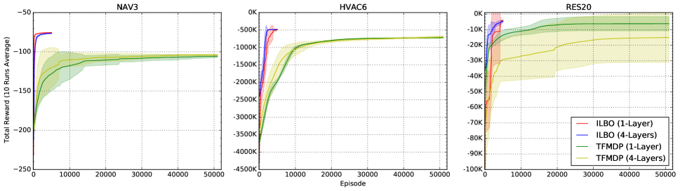
Figure 2: Total Reward Obtained (Higher is Better); $\operatorname{tfmdp}$ setting: 200 epochs; 256 Batchsize. x-axis denotes # episodes, y-axis quality

We also remark on the structure of expression (24). Gradient ascent tries to optimize the reward in the first term. In the second term, it tries to increase the probability of transitioning to highly-valued states. Since approximator $\hat{V}$ informs $\operatorname{ILBO}$ of the highly-valued states, gradient ascent on the transition function adjusts the policy such that it makes transition to highly rewarding states more likely. And the use of function approximator for state-action value function smooths out the effect of environment stochasticity as action-value function can be learned from past experiences also (explained later). These features of $\operatorname{ILBO}$ contribute to the sample efficiency and better quality solutions than $\operatorname{tfmdp}$. Another key difference between $\operatorname{ILBO}$ and $\operatorname{tfmdp}$ is that $\operatorname{ILBO}$ uses gradient of the transition function directly, whereas $\operatorname{tfmdp}$ encodes this information implicitly with reparameterization trick (Bueno et al. 2019).

Extension to continuous state spaces: Previous sections derived the MM formulation for a discrete state space MDP. We can also show how the MM formulation extends easily to the continuous state space also using Riemann sum based approximation of integrals in the continuous state space setting (proof in the supplemental material). The structure of the lower bound even in the continuous state setting remains the same as in (23) with summation over states replaced using an expectation over sampled states from the policy $\mu^{m}$.

Efficient utilization of samples: Notice that computing the gradient (24) requires on-policy samples, similar to $\operatorname{tfmdp}$. Therefore, we maintain a small store of recently observed episodes and use it to optimize the lower bound. However, our approach can still utilize samples from the past (or the so-called off-policy) samples to effectively train the state value estimate ${\hat{V}}_{\psi}(s)$ of the current policy. This makes our approach much more stable and sample efficient than $\operatorname{tfmdp}$ as our value function estimate is intuitively more accurate than estimating the value of a state only using on-policy samples from the current mini-batch of episodes as in $\operatorname{tfmdp}$. We provide more on such implementation details, and the entire $\operatorname{ILBO}$ algorithm in the supplementary.

5 Experiments

We present the empirical results comparing performance of $\operatorname{ILBO}$ against that of state-of-the-art DRP planner, $\operatorname{tfmdp}$ (Bueno et al. 2019). Experiments were carried out in the three planning domains used to evaluate $\operatorname{tfmdp}$ (Bueno et al. 2019). We only provide a brief description of these three domains here; for details we refer to (Bueno et al. 2019). Experiments in these three planning domains have been conducted using the Python simulator made publicly available on the RDDLGym GitHub repository (Bueno 2020). For $\operatorname{tfmdp}$, we used its Python implementation, available on GitHub (Bueno 2021).

Navigation is a path planning problem in a two-dimensional space (Faulwasser and Findeisen 2009). The agent’s location is encoded as a continuous state variable $\boldsymbol{s}_{t}\in\mathbb{R}^{2}$ while the continuous action variable $\boldsymbol{a}_{t}\in[-1,1]^{2}$ represents its movement magnitudes in the horizontal and vertical directions. The objective is to reach the goal state in the presence of deceleration zones.

HVAC control is a centralized planning problem where an agent controls the heated air to be supplied to each of the $N$ rooms (Agarwal et al. 2010). Continuous state variable $\boldsymbol{s}_{t}\in\mathbb{R}^{N}$ represents the temperature of each room and action variable $\boldsymbol{a}_{t}\in[0,a_{max}]^{N}$ is comprised of the amount of heated air supplied; $N=6$ in this domain. The objective is to maintain the room temperatures within the desired range.

Reservoir Reservoir management requires the planner to release water to downstream reservoirs to maintain the desired water level (Yeh 1985). State variable ${s}_{t}^{i}$  is the water level at reservoir $i$ and action variable ${a}_{t}^{i}\in[0,{s}_{t}^{i}]$ represents the water outflow to the downstream reservoir. A penalty is imposed if the reservoir level is too low or high. Both state and action spaces are 20-dimensional.

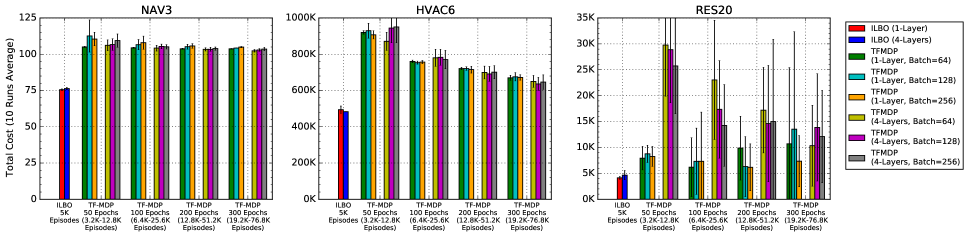
Figure 3: Total Cost Incurred by the Final Policy (Lower is Better); $\operatorname{tfmdp}$: Various Hyperparameter Settings

Experiment Objectives We assess $\operatorname{ILBO}$’s performance in the following aspects:

• Sample efficiency and quality of solution: The ability to provide high-quality solution (in terms of total rewards gathered) in a sample-efficient manner.

• Training stability: The policy network should gradually stabilize and not exhibit sudden large degradations in performance as learning progresses.

• Generalization capability: The ability to generalize to other problem instances (e.g., new initial states) without having to retrain.

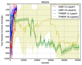
Figure 4: Total Reward Obtained by Current Policy in RES20 (Higher is Better); $\operatorname{tfmdp}$ setting: 200 epochs & 256 Batchsize

Hyperparameters We evaluated $\operatorname{ILBO}$ using two representative DRP architectures: one hidden layer and four hidden layers, exactly the same architectures used in the evaluation (Bueno et al. 2019). The total learning episodes for $\operatorname{ILBO}$ is 5000 in all our experiments. The default setting for $\operatorname{tfmdp}$ is: 200 epochs of 256 batchsize, where batchsize refers to the number of episodes (or trajectories) sampled per epoch (Bueno et al. 2019). We performed detailed comparisons with a variety of $\operatorname{tfmdp}$ hyperparameter settings: epoch = {50, 100, 200, 300}, batchsize = {64, 128, 256}. We refer the reader to supplement for other hyperparameter settings used in the experiments.

Performance Reporting We adopt the same approach as $\operatorname{tfmdp}$  (Bueno et al. 2019), which reports the average and standard deviation values over 10 training runs and for each training run, the best policy so far is kept to smooth out the effects of stochasticity during training. All the result figures report solution qualities attained by the best policies so far, with the exception of Figure 4, which compares the training stability of $\operatorname{ILBO}$ and $\operatorname{tfmdp}$. We use 64 test trajectories (different from training ones) to evaluate the policy.

Sample Efficiency, Quality The total rewards gathered by $\operatorname{ILBO}$ and $\operatorname{tfmdp}$ are shown in Figure 2 for all three domains. The two $\operatorname{tfmdp}$ curves were trained using the default settings specified in (Bueno et al. 2019): epoch = 200, batchsize = 256. Compared to $\operatorname{tfmdp}$, $\operatorname{ILBO}$ converges to higher quality plan earlier and collects much fewer sample episodes in all three domains. There are several key reasons for this. Our method can learn better estimate of state value function using off-policy samples, which intuitively is more accurate than estimating value function from only on-policy samples. For highly stochastic domains, such as reservoir, limited on-policy samples may not be enough to provide a reliable estimate of the value function. Additionally, the gradient in (24) can be estimated after collecting sufficient experience samples, without having to wait for full trajectory samples, which is required in $\operatorname{tfmdp}$. Consequently, $\operatorname{ILBO}$ is able to produce high quality plans in a sample-efficient manner over $\operatorname{tfmdp}$, as the empirical result suggests.

Training Stability From Figure 2, the reader may notice the large variance present in the total rewards gathered by $\operatorname{tfmdp}$ for Reservoir-20 domain. Compared to the other two domains, Reservoir-20 domain is highly stochastic and its transition dynamics is characterized by the Gamma distribution, which has fat tails at both ends. Consequently, each mini-batch of collected samples can be highly dissimilar. The effect of this high stochasticity on $\operatorname{ILBO}$ and $\operatorname{tfmdp}$ is further examined in Figure 4. Instead of remembering the best policy so far, this diagram shows the average total reward of current policies at every training step.

Figure 4 demonstrates that $\operatorname{ILBO}$ is more resilient to environment stochasticity. The weight updates by $\operatorname{ILBO}$ are more stable and the policy improves iteratively. In comparison, $\operatorname{tfmdp}$ witnesses large variations in policy performance towards the later part of training. We postulate that this is due to the better learning of value estimates by $\operatorname{ILBO}$. Although the environment is highly stochastic, $\operatorname{ILBO}$ updates value function using historical samples. As a result, this stochastic effect was smoothed out. In contrast, $\operatorname{tfmdp}$ only uses the current batch of trajectory samples to compute gradient updates. In a highly stochastic domain like Reservoir-20, one single batch might not contain sufficient number of representative trajectory samples. Consequently, $\operatorname{tfmdp}$ might estimate gradients using these unrepresentative samples, causing huge performance degradation.

Varying hyperparameters of $\boldsymbol{\operatorname{tfmdp}}$ The bar charts in Figure 3 quantify the total cost achieved at the end of training. This chart presents the full range of $\operatorname{tfmdp}$ performance across a variety of epoch and batchsize settings, in order to provide an elaborate comparison. Note that cost is defined as negative reward and hence lower is better in this figure.

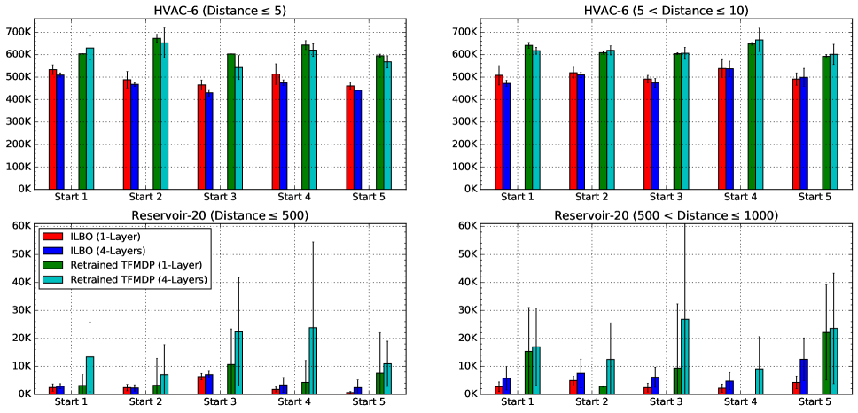
Figure 5: Total Cost Incurred in New Initial States (Lower is Better): Same $\operatorname{ILBO}$ Policy vs Retrained $\operatorname{tfmdp}$ Policy

In HVAC and Reservoir domains, increasing the number of epochs and/or batchsize improves the solution qualities attained by $\operatorname{tfmdp}$, albeit at the cost of sample efficiency. We continue to witness high variance in $\operatorname{tfmdp}$’s Reservoir-20 policy performance; this corroborates our finding in Figure 4. The best $\operatorname{tfmdp}$ policy in Reservoir domain is trained with 200 epochs of 256 batchsize. However, its high variance indicates that $\operatorname{tfmdp}$ often produces significantly worse policies in many of the runs.

In comparison, $\operatorname{ILBO}$ consistently produces higher quality solutions across all three domains, with significantly lower average total cost and variance. It is worth pointing our that even in the highly stochastic Reservoir domain, the performance variance of $\operatorname{ILBO}$ policies remain low. This is advantageous since it provides the assurance that $\operatorname{ILBO}$ consistently produces policies with similar performance, despite high stochasticity present in the environment.

Generalization The $\operatorname{tfmdp}$ algorithm estimates gradients from a fixed-length Stochastic Computation Graph (Schulman et al. 2015a) and the planning horizon is fixed before training commences. Coupled with fixed initial state, the training samples collected by agent may be too monotonous and disadvantage the DRP in generalizing to new states. In contrast, the better training of state value approximator coupled with explicitly taking gradients of reward and transition function in $\operatorname{ILBO}$ (24) helps $\operatorname{ILBO}$ to ride out the idiosyncrasy present within a single minibatch of samples, and generalize better to new states.

Figure 5 demonstrates $\operatorname{ILBO}$’s ability to generalize. We evaluated the same $\operatorname{ILBO}$ policies trained for the original start state in HVAC and Reservoir domains, without performing retraining. Ten different random start states were used in this evaluation. Five of them are within shorter Euclidean distance from the original start state while the other five are of larger distance. We retrained $\operatorname{tfmdp}$ in these new start states to serve as benchmark for comparison.

For HVAC-6 domain, $\operatorname{ILBO}$ consistently outperforms the retrained $\operatorname{tfmdp}$ in all ten start states. As for Res-20 domain, $\operatorname{ILBO}$ outperforms the retrained $\operatorname{tfmdp}$ in all but two initial states (i.e., Start 2 and Start 4 in the lower right chart). We postulate that this is because the state space is high-dimensional and very large in Res-20 domain, and the agent may not have collected sufficient representative transition samples within 5000 episodes. More training episodes would allow $\operatorname{ILBO}$ to improve generalization in the learned policy.

6 Conclusion and Future Work

In this work, we developed a novel minorization-maximization approach for sample-efficient deep reactive policy (DRP) learning in nonlinear CSA-MDPs using iterative lower bound optimization ($\operatorname{ILBO}$). Empirical results confirmed $\operatorname{ILBO}$’s superior sample efficiency, solution quality, stability, and generalization to new initial states by learning from diverse transition samples.

One interesting direction of future work would be to extend $\operatorname{ILBO}$ to other types of MDP problems such as constrained MDPs (Altman 1999; Feyzabadi and Carpin 2014). Solving constrained MDPs in a sample-efficient manner is particularly important in many safety-critical settings germane to the deployment of DRPs. Another promising direction would be to develop $\operatorname{ILBO}$ extensions for optimizing DRPs that are robust to model error (Nilim and El Ghaoui 2005; Wiesemann, Kuhn, and Rustem 2013), which would further facilitate their practical deployment when high fidelity models are hard to learn or acquire.

References

- Aberdeen (2005) Aberdeen, D. 2005. Policy-Gradient Methods for Planning. In Advances in Neural Information Processing Systems 18 [Neural Information Processing Systems, NIPS 2005, December 5-8, 2005, Vancouver, British Columbia, Canada], 9–16.
- Agarwal et al. (2010) Agarwal, Y.; Balaji, B.; Gupta, R.; Lyles, J.; Wei, M.; and Weng, T. 2010. Occupancy-Driven Energy Management for Smart Building Automation. In Proceedings of the 2nd ACM Workshop on Embedded Sensing Systems for Energy-Efficiency in Building, BuildSys ’10, 1–6. New York, NY, USA: Association for Computing Machinery. ISBN 9781450304580.
- Altman (1999) Altman, E. 1999. Constrained Markov decision processes, volume 7. CRC Press.
- Bajpai, Garg, and Mausam (2018) Bajpai, A. N.; Garg, S.; and Mausam. 2018. Transfer of Deep Reactive Policies for MDP Planning. In Bengio, S.; Wallach, H. M.; Larochelle, H.; Grauman, K.; Cesa-Bianchi, N.; and Garnett, R., eds., Advances in Neural Information Processing Systems 31: Annual Conference on Neural Information Processing Systems 2018, NeurIPS 2018, December 3-8, 2018, Montréal, Canada, 10988–10998.
- Bengio, Lecun, and Hinton (2021) Bengio, Y.; Lecun, Y.; and Hinton, G. 2021. Deep Learning for AI. Commun. ACM, 64(7): 58–65.
- Bertsekas (1999) Bertsekas, D. 1999. Nonlinear Programming. Athena Scientific.
- Boutilier, Dean, and Hanks (1999) Boutilier, C.; Dean, T. L.; and Hanks, S. 1999. Decision-Theoretic Planning: Structural Assumptions and Computational Leverage. Journal of Artificial Intelligence Research, 11: 1–94.
- Bueno (2020) Bueno, T. P. 2020. rddlgym. https://github.com/thiagopbueno/rddlgym. Accessed: 2021-09-07.
- Bueno (2021) Bueno, T. P. 2021. tf-mdp. https://github.com/thiagopbueno/tf-mdp. Accessed: 2021-09-07.
- Bueno et al. (2019) Bueno, T. P.; de Barros, L. N.; Mauá, D. D.; and Sanner, S. 2019. Deep Reactive Policies for Planning in Stochastic Nonlinear Domains. In AAAI Conference on Artificial Intelligence, 7530–7537.
- Buffet and Aberdeen (2007) Buffet, O.; and Aberdeen, D. 2007. FF + FPG: Guiding a Policy-Gradient Planner. In Boddy, M. S.; Fox, M.; and Thiébaux, S., eds., Proceedings of the Seventeenth International Conference on Automated Planning and Scheduling, ICAPS 2007, Providence, Rhode Island, USA, September 22-26, 2007, 42–48. AAAI.
- Buffet and Aberdeen (2009) Buffet, O.; and Aberdeen, D. 2009. The factored policy-gradient planner. Artificial Intelligence, 173(5): 722–747.
- Dempster, Laird, and Rubin (1977) Dempster, A. P.; Laird, N. M.; and Rubin, D. B. 1977. Maximum Likelihood from Incomplete Data via the EM Algorithm. Journal of the Royal Statistical Society. Series B (Methodological), 39(1): 1–38.
- Faulwasser and Findeisen (2009) Faulwasser, T.; and Findeisen, R. 2009. Nonlinear model predictive path-following control. In Nonlinear model predictive control, 335–343. Springer.
- Feyzabadi and Carpin (2014) Feyzabadi, S.; and Carpin, S. 2014. Risk-aware path planning using hirerachical constrained markov decision processes. In 2014 IEEE International Conference on Automation Science and Engineering (CASE), 297–303. IEEE.
- Garg, Bajpai, and Mausam (2019) Garg, S.; Bajpai, A.; and Mausam. 2019. Size Independent Neural Transfer for RDDL Planning. In Benton, J.; Lipovetzky, N.; Onaindia, E.; Smith, D. E.; and Srivastava, S., eds., Proceedings of the Twenty-Ninth International Conference on Automated Planning and Scheduling, ICAPS 2018, Berkeley, CA, USA, July 11-15, 2019, 631–636. AAAI Press.
- Garg, Bajpai, and Mausam (2020) Garg, S.; Bajpai, A.; and Mausam. 2020. Symbolic Network: Generalized Neural Policies for Relational MDPs. In Proceedings of the 37th International Conference on Machine Learning, ICML 2020, 13-18 July 2020, Virtual Event, volume 119 of Proceedings of Machine Learning Research, 3397–3407. PMLR.
- Groshev et al. (2018) Groshev, E.; Goldstein, M.; Tamar, A.; Srivastava, S.; and Abbeel, P. 2018. Learning Generalized Reactive Policies Using Deep Neural Networks. In de Weerdt, M.; Koenig, S.; Röger, G.; and Spaan, M. T. J., eds., Proceedings of the Twenty-Eighth International Conference on Automated Planning and Scheduling, ICAPS 2018, Delft, The Netherlands, June 24-29, 2018, 408–416. AAAI Press.
- Hinton et al. (2012) Hinton, G.; Deng, L.; Yu, D.; Dahl, G. E.; Mohamed, A.-r.; Jaitly, N.; Senior, A.; Vanhoucke, V.; Nguyen, P.; Sainath, T. N.; and Kingsbury, B. 2012. Deep Neural Networks for Acoustic Modeling in Speech Recognition: The Shared Views of Four Research Groups. IEEE Signal Processing Magazine, 29(6): 82–97.
- Hunter and Lange (2004) Hunter, D. R.; and Lange, K. 2004. A Tutorial on MM Algorithms. American Statistician, 58(1): 30–37.
- Issakkimuthu, Fern, and Tadepalli (2018) Issakkimuthu, M.; Fern, A.; and Tadepalli, P. 2018. Training Deep Reactive Policies for Probabilistic Planning Problems. In de Weerdt, M.; Koenig, S.; Röger, G.; and Spaan, M. T. J., eds., Proceedings of the Twenty-Eighth International Conference on Automated Planning and Scheduling, ICAPS 2018, Delft, The Netherlands, June 24-29, 2018, 422–430. AAAI Press.
- Krizhevsky, Sutskever, and Hinton (2017) Krizhevsky, A.; Sutskever, I.; and Hinton, G. E. 2017. ImageNet Classification with Deep Convolutional Neural Networks. Commun. ACM, 60(6): 84–90.
- Lange (2016) Lange, K. 2016. MM Optimization Algorithms. Society for Industrial and Applied Mathematics.
- Nilim and El Ghaoui (2005) Nilim, A.; and El Ghaoui, L. 2005. Robust Control of Markov Decision Processes with Uncertain Transition Matrices. Oper. Res., 53(5): 780–798.
- Raghavan et al. (2017) Raghavan, A.; Sanner, S.; Tadepalli, P.; Fern, A.; and Khardon, R. 2017. Hindsight Optimization for Hybrid State and Action MDPs. In Proceedings of the 31st AAAI Conference on Artificial Intelligence (AAAI-17). San Francisco, USA.
- Say (2021) Say, B. 2021. A Unified Framework for Planning with Learned Neural Network Transition Models. In AAAI Conference on Artificial Intelligence, AAAI, 5016–5024.
- Say et al. (2020) Say, B.; Devriendt, J.; Nordström, J.; and Stuckey, P. J. 2020. Theoretical and Experimental Results for Planning with Learned Binarized Neural Network Transition Models. In Principles and Practice of Constraint Programming, 917–934.
- Say and Sanner (2018) Say, B.; and Sanner, S. 2018. Planning in Factored State and Action Spaces with Learned Binarized Neural Network Transition Models. In International Joint Conference on Artificial Intelligence, 4815–4821.
- Scaroni et al. (2020) Scaroni, R.; Bueno, T. P.; de Barros, L. N.; and Mauá, D. 2020. On the Performance of Planning Through Backpropagation. In Cerri, R.; and Prati, R. C., eds., Intelligent Systems, 108–122. Springer International Publishing.
- Schulman et al. (2015a) Schulman, J.; Heess, N.; Weber, T.; and Abbeel, P. 2015a. Gradient estimation using stochastic computation graphs. In Advances in Neural Information Processing Systems, 3528–3536.
- Schulman et al. (2015b) Schulman, J.; Levine, S.; Moritz, P.; Jordan, M.; and Abbeel, P. 2015b. Trust region policy optimization. In International Conference on Machine Learning, volume 3, 1889–1897. ISBN 9781510810587.
- Toussaint and Storkey (2006) Toussaint, M.; and Storkey, A. J. 2006. Probabilistic inference for solving discrete and continuous state Markov Decision Processes. In International Conference on Machine Learning, 945–952.
- Toyer et al. (2020) Toyer, S.; Thiébaux, S.; Trevizan, F. W.; and Xie, L. 2020. ASNets: Deep Learning for Generalised Planning. J. Artif. Intell. Res., 68: 1–68.
- Toyer et al. (2018) Toyer, S.; Trevizan, F. W.; Thiébaux, S.; and Xie, L. 2018. Action Schema Networks: Generalised Policies With Deep Learning. In McIlraith, S. A.; and Weinberger, K. Q., eds., Proceedings of the Thirty-Second AAAI Conference on Artificial Intelligence, (AAAI-18), the 30th innovative Applications of Artificial Intelligence (IAAI-18), and the 8th AAAI Symposium on Educational Advances in Artificial Intelligence (EAAI-18), New Orleans, Louisiana, USA, February 2-7, 2018, 6294–6301. AAAI Press.
- Wiesemann, Kuhn, and Rustem (2013) Wiesemann, W.; Kuhn, D.; and Rustem, B. 2013. Robust Markov decision processes. Mathematics of Operations Research, 38(1): 153–183.
- Wu, Say, and Sanner (2017) Wu, G.; Say, B.; and Sanner, S. 2017. Scalable Planning with Tensorflow for Hybrid Nonlinear Domains. In Advances in Neural Information Processing Systems, 6273–6283.
- Wu, Say, and Sanner (2020) Wu, G.; Say, B.; and Sanner, S. 2020. Scalable Planning with Deep Neural Network Learned Transition Models. Journal of Artificial Intelligence Research, 68: 571–606.
- Yeh (1985) Yeh, W. 1985. Reservoir Management and Operations Models: A State‐of‐the‐Art Review. Water Resources Research, 21: 1797–1818.
- Zamani, Sanner, and Fang (2012) Zamani, Z.; Sanner, S.; and Fang, C. 2012. Symbolic Dynamic Programming for Continuous State and Action MDPs. In Hoffmann, J.; and Selman, B., eds., AAAI Conference on Artificial Intelligence.