Diagrammatic Monte Carlo for electronic correlation in molecules:
high-order many-body perturbation theory with low scaling

Abstract

We present a low-scaling diagrammatic Monte Carlo approach to molecular correlation energies. Using combinatorial graph theory to encode many-body Hugenholtz diagrams, we sample the Møller-Plesset (MP$n$) perturbation series, obtaining accurate correlation energies up to $n=5$, with quadratic scaling in the number of basis functions. Our technique reduces the computational complexity of the molecular many-fermion correlation problem, opening up the possibility of low-scaling, accurate stochastic computations for a wide class of many-body systems described by Hugenholtz diagrams.

The many-electron correlation energy, defined as the difference between the true energy of a many-electron system and that obtained in the Hartree-Fock (HF) approximation Szabo and Ostlund (1996); Bartlett and Musiał (2007); Shavitt and Bartlett (2009); Cremer (2011); Hirata et al. (2014); Tew et al. (2007), plays a central role in the theoretical description of a wide array of phenomena in chemistry, physics, and material science Szabo and Ostlund (1996); Martin et al. (2006); Tew et al. (2007) ranging from dispersion interactions responsible for protein folding He et al. (2009) and photoisomerization of retinal, the first step in vision Gozem et al. (2012); Liu et al. (2016) to strongly correlated many-electron states in transition-metal compounds Chan and Sharma (2011), and high-temperature superconductors Mueck (2015). The development of highly efficient computational methods for calculating the many-electron correlation energy is thus an ultimate goal of modern electronic structure theory Bartlett and Musiał (2007); Shavitt and Bartlett (2009); Martin et al. (2006).

Many-body perturbation theory (MBPT) Szabo and Ostlund (1996); Hirata et al. (2014) and coupled-cluster (CC) theory Bartlett and Musiał (2007) are the two primary methods for treating the effects of dynamic correlation, where a single HF state provides a qualitatively correct zeroth-order approximation to the electronic wavefunction Bartlett and Musiał (2007). Both MBPT and CC methods have been very successful in predicting the correlation energies of small and medium-size molecules Bartlett and Musiał (2007); Hirata et al. (2014), whereas second-order Møller-Plesset perturbation theory (MP2) Szabo and Ostlund (1996); Bartlett and Musiał (2007); Shavitt and Bartlett (2009) is the method of choice for calculating electron correlation effects in large systems involving thousands of atoms Hirata et al. (2014); Cremer (2011). Despite the well-documented shortcomings of higher-order MP$n$ methods ($n\gtrsim 3$) such as non-monotonous convergence Cremer (2011), with proper choice of orbitals and regularization, such methods can provide chemically accurate results not only for molecular energy differences, but also for reaction barrier heights and intermolecular interactions Bertels et al. (2019); Heßelmann (2019).

However, widespread application of MP$n$ and CC methods to larger molecules is limited by the steep scaling of the computational cost ($N^{n+3}$ in the case of MP$n$) with the number of spin-orbitals $N$ Cremer (2011); Hirata et al. (2014); Ratcliff et al. (2017). This problem has motivated the development of ingenious low-scaling methods Izmaylov and Scuseria (2008); Pulay (1983); Ayala et al. (2001); Werner et al. (2003); Izmaylov and Scuseria (2008); Neuhauser et al. (2013). Among those, several promising Monte Carlo (MC) techniques rely on stochastic sampling of configuration-interaction (CI) Thom and Alavi (2007); Booth et al. (2009) and CC Scott et al. (2019) expansions in imaginary time or performing real-space MC integration to obtain MP$n$ energies Willow et al. (2012); Willow and Hirata (2014); Hirata et al. (2014); Li (2019); Doran and Hirata (2021).

In this Letter, we introduce a novel stochastic approach to the many-electron correlation problem in molecules based on the powerful Diagrammatic Monte Carlo (DiagMC) methodology Prokof’ev and Svistunov (1998); Van Houcke et al. (2010); Gull et al. (2011), which uses direct sampling of the entire diagrammatic series for the many-electron correlation energy to obtain numerically results free of systematic bias. Originally developed in the context of quantum impurity problems Prokof’ev and Svistunov (1998); Gull et al. (2011), DiagMC has been applied with great success to a wide range of problems in quantum many-body physics, including exotic impurities with internal degrees of freedom Bighin and Lemeshko (2017); Bighin et al. (2018); Li et al. (2019, 2020a), correlated lattice fermions Kozik et al. (2010), unitary Fermi gases Van Houcke et al. (2012), and non-equilibrium quantum dynamics Cohen et al. (2015). Recent applications of the DiagMC approach have provided numerically exact correlation energies of the homogeneous electron gas Chen and Haule (2019) and of an infinite chain of hydrogen atoms Motta et al. (2017). Thus far, however, save for a very recent application to molecular quantum impurity problems at finite temperature Li et al. (2020b), DiagMC has not been applied to calculate molecular correlation energies, likely due to the topological complexity of the underlying Hugenholtz diagrams.

Here, we overcome this problem by using combinatorial graph theory to encode Hugenholtz diagrams into adjacency matrices, a technique recently developed in nuclear physics Tichai (2017); Arthuis et al. (2019). This allows us to design general and efficient updates for sampling the diagrammatic expansions of MBPT using the Metropolis algorithm. Unlike full configuration interaction MC Booth et al. (2009), stochastic MP$n$ theory in real space Willow et al. (2012); Willow and Hirata (2014); Hirata et al. (2014); Li (2019), or DiagMC for molecular quantum impurities Li et al. (2020b), our DiagMC/MP$n$ method evaluates the correlation energy directly based on a random walk in the space of Hugenholtz diagrams, rather than that of Slater determinants or in real space.

We apply our approach to calculate the correlation energies of small molecules, obtaining accurate MP$n$ results up to $n=4$ with low $O(N^{2})$ scaling, opening up the possibility of accessing heretofore unexplored regimes in the upper right corner of the Pople diagram Pople (1965); Karplus (1990) – i.e., computing accurate dynamical correlation energies for much larger systems than was previously possible. Because our methodology only relies on graph theory, it can be easily extended beyond electronic structure theory to include the diagrammatic expansions that occur in, e.g., vibrational spectroscopy Hermes and Hirata (2013, 2014); Hirata et al. (2015), crystal phonon perturbation theory Cowley (1963); Goldman et al. (1968); Koehler (1969), and nuclear physics Tichai (2017); Arthuis et al. (2019).

MPn theory and matrix encoding of Hugenholtz diagrams.

In MP$n$ theory Hirata et al. (2014); Shavitt and Bartlett (2009); Cremer (2011), the non-relativistic electronic Hamiltonian $\hat{H}=\sum\varepsilon_{i}\hat{c}_{i}^{\dagger}\hat{c}_{i}+\frac{1}{2}\sum_{ijkl}\langle ij||kl\rangle\hat{c}^{\dagger}_{i}\hat{c}_{j}^{\dagger}\hat{c}_{l}\hat{c}_{k}$ is partitioned into the mean-field reference Hamiltonian $\hat{H}_{0}=\sum_{i}\varepsilon_{i}\hat{c}_{i}^{\dagger}\hat{c}_{i}$ plus a fluctuation potential $\hat{V}=\hat{H}-\hat{H}_{0}$, where $\varepsilon_{i}$ are the HF orbital energies, $\hat{c}_{i}^{\dagger}$ ($\hat{c}_{i}$) are the creation (annihilation) operators for the electron in the $i$-th HF spin-orbital, respectively, and $\langle ij||kl\rangle$ are the antisymmetrized two-electron repulsion integrals (ERIs) Szabo and Ostlund (1996). The correlation energy is given by the Rayleigh-Schrödinger perturbation series including only the linked terms Goldstone and Mott (1957); Shavitt and Bartlett (2009),

$$E_{\text{c}}=E-E_{\text{HF}}=\sum_{m=0}\langle\hat{V}(\hat{R}_{0}\hat{V})^{m}\rangle_{L},$$ (1)

where $\hat{R}_{0}=(1-|\Phi_{0}\rangle\langle\Phi_{0}|)(z-\hat{H}_{0})^{-1}$ is the reduced resolvent operator for the HF reference state $|\Phi_{0}\rangle$ Shavitt and Bartlett (2009); Kutzelnigg (2009).

The different terms in the MP$n$ series of Eq. (1) are most compactly represented by means of Hugenholtz diagrams Negele and Orland (1988); Szabo and Ostlund (1996). Diagrams contributing to the $n$-order consist of $n$ labeled vertices, vertically aligned by convention. Each vertex corresponds to an ERI $\langle ij||kl\rangle$ and has two incoming and two outgoing lines, corresponding to either particle orbitals $a,b,c,\ldots$ (upward lines) or hole orbitals $r,s,t,\ldots$ (downward lines) Shavitt and Bartlett (2009). Additionally, diagrams with different line orientations are considered distinct, a line cannot start and end on the same vertex, each diagram must consist of only one connected component, and its overall sign $s=(-1)^{h-l}$ depends on the number of holes $h$ and of closed loops $l$. Each pair of adjacent vertices contributes the factor $(\sum_{h}\varepsilon_{h}-\sum_{p}\varepsilon_{p})^{-1}$, where the sums run over the particles and holes crossing an imaginary horizontal line between the vertices. Finally, each diagram is scaled by $2^{-p}$, $p$ being the number of equivalent line pairs (i.e., co-directed lines that start and end on the same vertex) Shavitt and Bartlett (2009). The number of $n$-th order Hugenholtz diagrams grows factorially with $n$ Sloane (2020). Representative $n=2{-}4$ diagrams are shown in Fig. 1. Our DiagMC approach presented below directly samples the expansion of the correlation energy (1) in terms of Hugenholtz diagrams.

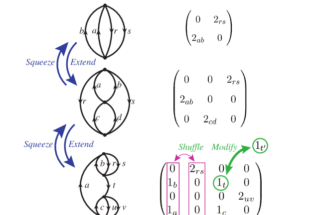
Figure 1: Representative Hugenholtz diagrams contributing to the $n$-order of MP theory with $n=2$, 3, and 4 along with their corresponding adjacency matrices Tichai (2017); Arthuis et al. (2019) shown to the right of each diagram. The different types of DiagMC updates are indicated by blue arrows (for Extend and Squeeze), by magenta arrows (for Shuffle), and by green arrows (for Modify), see main text for details.

We now observe, following recent work on MBPT in nuclear physics Tichai (2017); Arthuis et al. (2019) that, according to graph theory, Hugenholtz diagrams of order $n$ can be conveniently encoded into $n\times n$ adjacency matrices that satisfy the following conditions: (i) $A_{ij}$ can only take values 0, 1, 2, (ii) $\sum_{i}A_{ij}=2\ \forall j$, (iii) $\sum_{j}A_{ij}=2\ \forall i$, and (iv) $A_{ii}=0\ \forall i$. Fig. 1(b) shows the adjacency matrix representations of selected MP$n$ diagrams. We stress that in some contexts one names ‘diagram’ the summed-over expression, after the sums over the hole and particle indices have been carried out. Here, we call ‘diagram’ an expression depending on these indices, with no sum implied. We make this apparent by introducing appropriate subscript indices on the entries of the matrices of Fig. 1; the diagrammatic rules above, along with the convention we choose for the adjacency matrix, imply that entries below (above) the diagonal will carry hole (particle) indices, respectively. The core idea of the present Letter is to stochastically sample these diagrams – through their matrix representation – at all orders, varying the topology of the diagram and the value of the indices Prokof’ev and Svistunov (1998); Mishchenko et al. (2000); Gukelberger et al. (2017); Van Houcke et al. (2019), converging – in the statistical sense – to the exact correlation energy.

For this purpose, we start by relaxing condition (iv) above, considering a larger set of matrices that have $A_{ii}\neq 0$. Within this extended configuration space $\mathcal{E}$, we distinguish between physical matrices – satisfying all four conditions – and unphysical ones – satisfying only conditions (i)-(iii) above. It can be shown SM that each matrix in $\mathcal{E}$ can be represented as the sum of two $N\times N$ permutation matrices $P$ defined by the following conditions (1) Each $P_{ij}=0$ or 1, (2) $\sum_{i}P_{ij}=1\ \forall j$, and (3) $\sum_{j}P_{ij}=1\ \forall i$. The converse is also, more trivially, true: two permutation matrices always sum to a matrix in $\mathcal{E}$. Therefore, the configuration space $\mathcal{E}$ consists essentially of two copies of the permutation matrix configuration space. As a consequence, we can just design a stochastic process sampling in the permutation matrix configuration space, subsequently ‘doubling’ it to sample over $\mathcal{E}$.

DiagMC procedure.

We now apply the DiagMC methodology Prokof’ev and Svistunov (1998); Mishchenko et al. (2000) by devising a set of updates that can ergodically explore the space of permutation matrices. The Extend${}_{\textit{1}}$ update adds a row to the bottom and a column to the right of a permutation matrix, thereby going from order $N$ to order $N+1$. We begin by choosing a non-zero entry $P_{ij}$ of the original matrix, setting it to zero, and subsequently ‘projecting’ it onto the newly created column and row. More specifically, we add two new entries $P_{(N+1)j}=1$ and $P_{i(N+1)}=1$. Due to the conventions discussed above, $P_{i(N+1)}$ will carry a hole index, while $P_{(N+1)j}$ will carry a particle index. We then reuse the numerical value of the index of the erased entry $P_{ij}$ as the index carried by one of the two new entries. Depending whether the old value was a particle or hole index, we will need to choose from a discrete uniform random distribution a new hole or particle index, respectively. The probability for this update is then

$$\mathcal{P}_{\textit{Extend}_{\textit{1}}}=\begin{cases}\frac{1}{N\ n_{\text{p}}}&\mathrm{if}\mbox{ }i\leq j\\ \frac{1}{N\ n_{\text{h}}}&\mathrm{otherwise}\end{cases}$$ (2)

where $n_{\text{h}}$ ($n_{\text{p}}$) is the total number of hole (particle) orbitals in the basis set being used, respectively. For the complementary update, that we denote Squeeze${}_{\textit{1}}$, we need to remove the two elements on the last row and column. There is just one way of doing so. Then we need to restore the $P_{ij}$ matrix element whose index might correspond either to a hole or to a particle state, and we can get the numerical value of that index from the index of one of the removed entries. The probability is then, $\mathcal{P}_{\textit{Squeeze}_{\textit{1}}}=1$.

The Extend${}_{\textit{2}}$ update adds one column and one row to a permutation matrix, and adds a new ‘1’ entry on the diagonal, on the bottom right. This will always take us to the unphysical sector, and by convention the newly added entry will always carry a hole index. The value is then drawn from a uniform random distribution, and the probability is then $\mathcal{P}_{\textit{Extend}_{\textit{2}}}=1/n_{\text{h}}$. The complementary Squeeze${}_{\textit{2}}$ update simply deletes the matrix element in the bottom right corner, returning to an $N\times N$ matrix. There are no probability distributions involved in this process, therefore one has $\mathcal{P}_{\textit{Squeeze}_{\textit{2}}}=1$.

In the Shuffle update, we first decide if we want to shuffle rows or columns. We then choose two random rows or column ands swap them. In doing so, the update might need to replace a hole index with a particle one or vice-versa, thus requiring to draw numbers from a uniform distribution. However, since the update is clearly self-complementary, one does not need to keep track of the associated probabilities, since the acceptance ratio depends on weight ratios only.

Lastly, we design a Modify update, in which a non-zero hole or particle entry is selected and the associated index is changed to a different value chosen from a uniform distribution. This update is also self-complementary Prokof’ev and Svistunov (1998); Mishchenko et al. (2000); Gukelberger et al. (2017); Van Houcke et al. (2019).

It is easily seen that the set of updates just introduced is ergodic. We then consider two permutation matrices and we apply the updates just introduced to each matrix at each MC step, with the constraint that the two matrices must always have the same dimension. In the spirit of DiagMC, we accept or reject the updates with a probability chosen as to make the process satisfy a detailed balance condition Prokof’ev and Svistunov (1998); Mishchenko et al. (2000); Gukelberger et al. (2017); Van Houcke et al. (2019); this implies that in the long run the process will spend with each diagram a number of MC steps proportional to the diagram weight, allowing us to collect statistics about the ratio of energies at different orders. The process jumps back and forth between the physical and unphysical sectors, the latter not contributing to the sampled quantities Gukelberger et al. (2017); Van Houcke et al. (2019). We verified that at every order the fraction of physical diagrams is always substantially large, moreover an arbitrary unphysical penalty dividing the weight of unphysical diagrams can help in tipping the balance towards the physical sector Gukelberger et al. (2017); Van Houcke et al. (2019).

We finally note that there are several distinct ways, in which a given adjacency matrix $\mathcal{A}$ can be represented as a sum of permutation matrices. We will call the number of such ways the multiplicity of $\mathcal{A}$. Since the multiplicity is not always one, some diagrams can be incorrectly ‘counted’ more than once. To avoid this spurious multiple-counting we simply divide the weight associated to a matrix by its multiplicity. An algorithmic determination of the multiplicity is presented in the Supplemental Material SM .

Table 1: Calculated correlation energies (in $\mu E_{h}$) for BH and $\mathrm{H}_{2}\mathrm{O}$ in the 6-31G basis set compared with the reference MP$n$ data from the Psi4 code.

Molecule	MP order $n$	DiagMC (this work)	Exact
BH	2	$-38.983338\pm 0.007937$	$-38.993128$
	3	$-13.297859\pm 0.004215$	$-13.301207$
	4	$-5.726406\pm 0.022243$	$-5.728702$
	5	$-2.664634\pm 0.050187$	$-2.779645$
H2O	2	$-129.050784\pm 0.025138$	$-129.053394$
	3	$-1.550238\pm 0.010480$	$-1.554750$
	4	$-5.110730\pm 0.052355$	$-5.247546$

Results: correlation energies and scaling.

As a first application of the proposed DiagMC/MP$n$ methodology, we carry out proof-of-principle computations on the CH₂, H₂O, and BH molecules and compare the results with reference MP$n$ calculations to assess the accuracy of the approach. This choice of molecules allows us to explore the performance of the DiagMC/MP$n$ approach for different convergence patterns of the MP$n$ series. While CH₂ and $\mathrm{B}\mathrm{H}$ are type-A molecules, for which the series converges monotonically, H₂O belongs to type B, exhibiting oscillating convergence Cremer and He (1996); Leininger et al. (2000).

We observe that the DiagMC/MP$n$ correlation energies listed in Table I and shown in Fig. 2(a-b), calculated using $10^{12}$ MC steps per data point, are in excellent agreement with the reference MP$n$ data computed using Psi4 Parrish et al. (2017), which validates all of the elements of our DiagMC procedure described above, regardless of the convergence pattern of the MP$n$ series. While the error in the DiagMC/MP$n$ correlation energy depends on the molecule and basis set used, it exhibits the expected statistical scaling $1/\sqrt{N_{\text{MC}}}$ with the number of MC steps, see Fig. 2(c). Figure 2(d) and the inset show that, for a fixed $N_{\text{MC}}$, the error increases approximately linearly as the basis set size is increased from the smallest (STO-3G) to the largest (6-31^∗∗G). This leads to the overall $O(N^{2})$ scaling of the computational effort in our approach with respect to the number of basis states, which makes it much more attractive computationally than conventional MP$n$ ($N^{n+3}$).

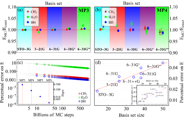
Figure 2: (a-b) MP3 and MP4 energies as calculated from our DiagMC procedure for $\mathrm{C}\mathrm{H}_{2}$, $\mathrm{H}_{2}\mathrm{O}$ and $\mathrm{B}\mathrm{H}$ molecules and for the STO-3G, 3-21G, 6-31G, 6-31^∗G, 6-31^∗∗G basis sets, performing $10^{12}$ MC steps per data point. (c) Percentual error on the energy as a function of the number of MC iterations, note the logarithmic scale; the black dashed lines guide the eye and corresponds to statistical $1/\sqrt{N_{\text{MC}}}$ scaling. Inset: expectation value of the sign as a function of the MP order, notice the logarithmic scale on the vertical axis. (d) Percentual error as a function of the basis size for the $\mathrm{BH}$ molecule after $10^{12}$ MC steps. The red dashed line guides the eyes, highlighting the essentially linear scaling. Main plot shows results at MP3 level, inset at MP4 level.

Sign problem.

Some of the diagrams we sample have negative weight, therefore we sample with respect to the absolute value of the diagram weight $\mathcal{D}_{\xi}$ Gull and Troyer (2013). Doing so, we observe that the statistical error in DiagMC/MP$n$ correlation energies grows significantly with increasing order $n$. This is due to the fermion sign problem, whereby the Hugenholtz diagrams with opposite signs cancel out, making it necessary to use an increasingly large number of MC steps to obtain a nonzero signal-to-noise ratio Landau and Binder (2000); Loh et al. (1990); Chandrasekharan and Wiese (1999). For instance, the contributions to the MP6 energy for the NH molecule using the 6-31G basis set and $10^{9}$ MC steps are estimated to be $0.342020\pm 0.001172$ and $0.342260\pm 0.001262$, respectively, with a sensibly increased error when the two values are subtracted to calculate the actual MP6 energy . We have also investigated this analytically, verifying that several topologies are dominated by near-perfect cancellations.

This phenonomenon, bearing a remarkable resemblance with the sign problem observed in other contexts Prokof’ev and Svistunov (2008); Kozik et al. (2010); Van Houcke et al. (2010, 2012); Vlietinck et al. (2014); Van Houcke et al. (2019) is, however, distinct from – and less severe than – the one that plagues quantum many-body MC simulations of, e.g., Fermi-Hubbard models. There, one is interested in the thermodynamic limit, and the expectation value of the sign decreases exponentially with the size of the system Landau and Binder (2000); Chandrasekharan and Wiese (1999); Loh et al. (1990). In contrast, for finite-size molecules explored here, this expectation value is small, decreases exponentially with the perturbation theory order, but is always finite, as shown in the inset of Fig. 2(c), significantly reducing the acuity of the sign problem. More in detail, here the sign problem is completely absent in MP2, quite moderate in MP3, and largely caused by the singles and triples contributions in MP4, see SM for a detailed analysis. There we also analyze how the the main idea behind the CDet algorithm Rossi et al. (2017) could lead to a substantial mitigation of the sign problem in the present context.

Outlook and conclusions.

We have demonstrated a low-scaling stochastic approach to calculating molecular electronic correlation energies based on DiagMC sampling of the MP$n$ series. The approach samples the many-body electronic correlation energy directly using Hugenholtz diagrams, encoded in adjacency matrices using combinatorial graph theory Arthuis et al. (2019). Our DiagMC/MP$n$ approach shares many of the attractive features with its antecedents in quantum many-body physics Prokof’ev and Svistunov (1998); Van Houcke et al. (2010), such as low scaling and the ability to converge towards the exact result (the full CI limit). We demonstrate accurate results for the MP$n$ correlation energies with $n\lesssim 5$. Already at MP4 level, the accuracy of our results is comparable to those provided by the CCSD(T) approach (the “golden standard” of quantum chemistry Bartlett and Musiał (2007); Heßelmann (2019)). Thus, our low-scaling DiagMC/MP$n$ methodology could be applied to a wide range of quantum chemical problems, where high-precision estimates of dynamical correlation energy are crucial, such as calculating intermolecular dispersion interactions Heßelmann (2019).

We find that results for $n\gtrsim 5$ are affected by the sign problem, which, however, is significantly less severe than the sign problem encountered in the thermodynamic limit Loh et al. (1990); Landau and Binder (2000) due to the finite size of molecular systems. In future work, we plan to address this problem adapting the recently-developed CDet algorithm Rossi et al. (2017, 2018). This would enable one to perform reliable extrapolations to the full CI limit Cremer and He (1996), using, e.g., Padé approximants, resummation techniques, and Feenberg scaling Cremer (2011), and to explore the convergence behavior of the MP$n$ series for large molecules, currently outside of reach of modern quantum chemistry techniques. Thus far, the behavior of the MP$n$ series for large $n$ has been explored only for the smallest molecules, for which full CI calculations could be performed Leininger et al. (2000).

References

- Szabo and Ostlund (1996) A. Szabo and N. S. Ostlund, Modern Quantum Chemistry: Introduction to Advanced Electronic Structure Theory, Dover Books on Chemistry (Dover Publications, 1996).
- Bartlett and Musiał (2007) R. J. Bartlett and M. Musiał, Rev. Mod. Phys. 79, 291 (2007).
- Shavitt and Bartlett (2009) I. Shavitt and R. J. Bartlett, Many-Body Methods in Chemistry and Physics: MBPT and Coupled-Cluster Theory (Cambridge University Press, Cambridge, 2009).
- Cremer (2011) D. Cremer, WIREs Comput. Mol. Sci. 1, 509 (2011).
- Hirata et al. (2014) S. Hirata, X. He, M. R. Hermes, and S. Y. Willow, J. Phys. Chem. A 118, 655 (2014).
- Tew et al. (2007) D. P. Tew, W. Klopper, and T. Helgaker, J. Comput. Chem. 28, 1307 (2007).
- Martin et al. (2006) R. Martin, L. Reining, and D. M. Ceperley, Interacting Electrons. Theory and Computational Approaches (Cambridge University Press, Cambridge, 2006).
- He et al. (2009) X. He, L. Fusti-Molnar, G. Cui, and K. M. Merz, J. Phys. Chem. B 113, 5290 (2009).
- Gozem et al. (2012) S. Gozem, M. Huntress, I. Schapiro, R. Lindh, A. A. Granovsky, C. Angeli, and M. Olivucci, J. Chem. Theory Comput. 8, 4069 (2012).
- Liu et al. (2016) L. Liu, J. Liu, and T. J. Martinez, J. Phys. Chem. B 120, 1940 (2016).
- Chan and Sharma (2011) G. K.-L. Chan and S. Sharma, Annu. Rev. Phys. Chem. 62, 465 (2011).
- Mueck (2015) L. Mueck, Nat. Chem. 7, 361 (2015).
- Bertels et al. (2019) L. W. Bertels, J. Lee, and M. Head-Gordon, J. Phys. Chem. Lett. 10, 4170 (2019).
- Heßelmann (2019) A. Heßelmann, J. Chem. Phys. 151, 114105 (2019).
- Ratcliff et al. (2017) L. E. Ratcliff, S. Mohr, G. Huhs, T. Deutsch, M. Masella, and L. Genovese, WIREs Comput. Mol. Sci. 7, e1290 (2017).
- Izmaylov and Scuseria (2008) A. F. Izmaylov and G. E. Scuseria, Phys. Chem. Chem. Phys. 10, 3421 (2008).
- Pulay (1983) P. Pulay, Chem. Phys. Lett. 100, 151 (1983).
- Ayala et al. (2001) P. Y. Ayala, K. N. Kudin, and G. E. Scuseria, J. Chem. Phys. 115, 9698 (2001).
- Werner et al. (2003) H.-J. Werner, F. R. Manby, and P. J. Knowles, J. Chem. Phys. 118, 8149 (2003).
- Neuhauser et al. (2013) D. Neuhauser, E. Rabani, and R. Baer, J. Chem. Theory Comput. 9, 24 (2013).
- Thom and Alavi (2007) A. J. W. Thom and A. Alavi, Phys. Rev. Lett. 99, 143001 (2007).
- Booth et al. (2009) G. H. Booth, A. J. W. Thom, and A. Alavi, J. Chem. Phys. 131, 054106 (2009).
- Scott et al. (2019) C. J. C. Scott, R. Di Remigio, T. D. Crawford, and A. J. W. Thom, J. Phys. Chem. Lett. 10, 925 (2019).
- Willow et al. (2012) S. Y. Willow, K. S. Kim, and S. Hirata, J. Chem. Phys. 137, 204122 (2012).
- Willow and Hirata (2014) S. Y. Willow and S. Hirata, J. Chem. Phys. 140, 024111 (2014).
- Li (2019) Z. Li, J. Chem. Phys. 151, 244114 (2019).
- Doran and Hirata (2021) A. E. Doran and S. Hirata, J. Chem. Phys. 154, 134114 (2021).
- Prokof’ev and Svistunov (1998) N. V. Prokof’ev and B. V. Svistunov, Phys. Rev. Lett. 81, 2514 (1998).
- Van Houcke et al. (2010) K. Van Houcke, E. Kozik, N. Prokof’ev, and B. Svistunov, Physics Procedia 6, 95 (2010).
- Gull et al. (2011) E. Gull, A. J. Millis, A. I. Lichtenstein, A. N. Rubtsov, M. Troyer, and P. Werner, Rev. Mod. Phys. 83, 349 (2011).
- Bighin and Lemeshko (2017) G. Bighin and M. Lemeshko, Phys. Rev. B 96, 085410 (2017).
- Bighin et al. (2018) G. Bighin, T. V. Tscherbul, and M. Lemeshko, Phys. Rev. Lett. 121, 165301 (2018).
- Li et al. (2019) X. Li, G. Bighin, E. Yakaboylu, and M. Lemeshko, Molecular Physics 117, 1981 (2019).
- Li et al. (2020a) X. Li, E. Yakaboylu, G. Bighin, R. Schmidt, M. Lemeshko, and A. Deuchert, The Journal of Chemical Physics 152, 164302 (2020a), https://doi.org/10.1063/1.5144759 .
- Kozik et al. (2010) E. Kozik, K. Van Houcke, E. Gull, L. Pollet, N. Prokof’ev, B. Svistunov, and M. Troyer, EPL (Europhysics Letters) 90, 10004 (2010).
- Van Houcke et al. (2012) K. Van Houcke, F. Werner, E. Kozik, N. Prokof’ev, B. Svistunov, M. J. H. Ku, A. T. Sommer, L. W. Cheuk, A. Schirotzek, and M. W. Zwierlein, Nature Physics 8, 366 (2012).
- Cohen et al. (2015) G. Cohen, E. Gull, D. R. Reichman, and A. J. Millis, Physical Review Letters 115, 266802 (2015).
- Chen and Haule (2019) K. Chen and K. Haule, Nat. Commun. 10, 769 (2019).
- Motta et al. (2017) M. Motta, D. M. Ceperley, G. K.-L. Chan, J. A. Gomez, E. Gull, S. Guo, C. A. Jiménez-Hoyos, T. N. Lan, J. Li, F. Ma, A. J. Millis, N. V. Prokof’ev, U. Ray, G. E. Scuseria, S. Sorella, E. M. Stoudenmire, Q. Sun, I. S. Tupitsyn, S. R. White, D. Zgid, and S. Zhang (Simons Collaboration on the Many-Electron Problem), Phys. Rev. X 7, 031059 (2017).
- Li et al. (2020b) J. Li, M. Wallerberger, and E. Gull, Phys. Rev. Research 2, 033211 (2020b).
- Tichai (2017) A. Tichai, Many-Body Perturbation Theory for Ab Initio Nuclear Structure, Ph.D. thesis, University of Darmstadt (2017).
- Arthuis et al. (2019) P. Arthuis, T. Duguet, A. Tichai, R. D. Lasseri, and J. P. Ebran, Comp. Phys. Commun. 240, 202 (2019).
- Pople (1965) J. A. Pople, J. Chem. Phys. 43, S229 (1965).
- Karplus (1990) M. Karplus, J. Phys. Chem. 94, 5435 (1990).
- Hermes and Hirata (2013) M. R. Hermes and S. Hirata, J. Chem. Phys. 139, 034111 (2013).
- Hermes and Hirata (2014) M. R. Hermes and S. Hirata, J. Chem. Phys. 141, 084105 (2014).
- Hirata et al. (2015) S. Hirata, M. R. Hermes, J. Simons, and J. V. Ortiz, J. Chem. Theory Comput. 11, 1595 (2015).
- Cowley (1963) R. A. Cowley, Adv. Phys. 12, 421 (1963).
- Goldman et al. (1968) V. V. Goldman, G. K. Horton, and M. L. Klein, Phys. Rev. Lett. 21, 1527 (1968).
- Koehler (1969) T. R. Koehler, Phys. Rev. Lett. 22, 777 (1969).
- Goldstone and Mott (1957) J. Goldstone and N. F. Mott, Proc. R. Soc. London Ser. A 239, 267 (1957).
- Kutzelnigg (2009) W. Kutzelnigg, Int. J. Quant. Chem. 109, 3858 (2009).
- Negele and Orland (1988) J. W. Negele and H. Orland, Quantum many-particle systems, Frontiers in physics (Addison-Wesley Pub. Co., 1988).
- Sloane (2020) N. J. A. Sloane, “Number of labeled hugenholtz diagrams with n nodes.” (2020), in: The On-line Encyclopedia of Integer Sequences.
- Mishchenko et al. (2000) A. S. Mishchenko, N. V. Prokof’ev, A. Sakamoto, and B. V. Svistunov, Physical Review B 62, 6317 (2000).
- Gukelberger et al. (2017) J. Gukelberger, E. Kozik, and H. Hafermann, Physical Review B 96, 035152 (2017).
- Van Houcke et al. (2019) K. Van Houcke, F. Werner, T. Ohgoe, N. V. Prokof’ev, and B. V. Svistunov, Physical Review B 99, 035140 (2019).
- (58) See Supplemental Material at [URL] for a detailed description of the properties of the matrices encoding Hugenholtz diagrams, as well as an extended discussion of the sign problem in the present context.
- Cremer and He (1996) D. Cremer and Z. He, J. Phys. Chem. 100, 6173 (1996).
- Leininger et al. (2000) M. L. Leininger, W. D. Allen, H. F. Schaefer, and C. D. Sherrill, J. Chem. Phys. 112, 9213 (2000).
- Parrish et al. (2017) R. M. Parrish, L. A. Burns, D. G. A. Smith, A. C. Simmonett, A. E. DePrince, E. G. Hohenstein, U. Bozkaya, A. Y. Sokolov, R. Di Remigio, R. M. Richard, J. F. Gonthier, A. M. James, H. R. McAlexander, A. Kumar, M. Saitow, X. Wang, B. P. Pritchard, P. Verma, H. F. Schaefer, K. Patkowski, R. A. King, E. F. Valeev, F. A. Evangelista, J. M. Turney, T. D. Crawford, and C. D. Sherrill, Journal of Chemical Theory and Computation 13, 3185 (2017).
- Gull and Troyer (2013) E. Gull and M. Troyer, in Strongly Correlated Systems, edited by A. Avella and F. Mancini (Springer Berlin Heidelberg, Berlin, Heidelberg, 2013).
- Landau and Binder (2000) D. Landau and K. Binder, A Guide to Monte Carlo Simulations in Statistical Physics (Cambridge University Press, 2000).
- Loh et al. (1990) E. Y. Loh, J. E. Gubernatis, R. T. Scalettar, S. R. White, D. J. Scalapino, and R. L. Sugar, Phys. Rev. B 41, 9301 (1990).
- Chandrasekharan and Wiese (1999) S. Chandrasekharan and U.-J. Wiese, Phys. Rev. Lett. 83, 3116 (1999).
- Note (1) All the errors on MC quantities we report throughout this Letter have been determined by means of a jackknife analysis, using the ALEA library from the ALPSCore package Bauer et al. (2011); Gaenko et al. (2017); Wallerberger et al. (2018).
- Prokof’ev and Svistunov (2008) N. Prokof’ev and B. Svistunov, Physical Review B 77, 020408(R) (2008).
- Vlietinck et al. (2014) J. Vlietinck, J. Ryckebusch, and K. Van Houcke, Physical Review B 89, 085119 (2014).
- Rossi et al. (2017) R. Rossi, N. Prokof’ev, B. Svistunov, K. Van Houcke, and F. Werner, EPL (Europhysics Letters) 118, 10004 (2017).
- Rossi et al. (2018) R. Rossi, T. Ohgoe, E. Kozik, N. Prokof’ev, B. Svistunov, K. Van Houcke, and F. Werner, Phys. Rev. Lett. 121, 130406 (2018).
- Tange (2021) O. Tange, “Gnu parallel 20220122 (’20 years’),” (2021), GNU Parallel is a general parallelizer to run multiple serial command line programs in parallel without changing them.
- Bauer et al. (2011) B. Bauer, L. D. Carr, H. G. Evertz, A. Feiguin, J. Freire, S. Fuchs, L. Gamper, J. Gukelberger, E. Gull, S. Guertler, A. Hehn, R. Igarashi, S. V. Isakov, D. Koop, P. N. Ma, P. Mates, H. Matsuo, O. Parcollet, G. Pawłowski, J. D. Picon, L. Pollet, E. Santos, V. W. Scarola, U. Schollwöck, C. Silva, B. Surer, S. Todo, S. Trebst, M. Troyer, M. L. Wall, P. Werner, and S. Wessel, Journal of Statistical Mechanics: Theory and Experiment 2011, P05001 (2011).
- Gaenko et al. (2017) A. Gaenko, A. Antipov, G. Carcassi, T. Chen, X. Chen, Q. Dong, L. Gamper, J. Gukelberger, R. Igarashi, S. Iskakov, M. Könz, J. LeBlanc, R. Levy, P. Ma, J. Paki, H. Shinaoka, S. Todo, M. Troyer, and E. Gull, Computer Physics Communications 213, 235 (2017).
- Wallerberger et al. (2018) M. Wallerberger, S. Iskakov, A. Gaenko, J. Kleinhenz, I. Krivenko, R. Levy, J. Li, H. Shinaoka, S. Todo, T. Chen, X. Chen, J. P. F. LeBlanc, J. E. Paki, H. Terletska, M. Troyer, and E. Gull, arXiv.org (2018), 1811.08331v1 .