The dark side of the proton

Abstract

We study the sensitivity of the High-Luminosity LHC to a light baryonic dark photon $B$, primarily coupled to quarks, as a constituent of the proton. This is achieved by allowing for a dark photon parton distribution function (PDF) in the PDF evolution equations. Depending on the mass and coupling of the dark photon, the evolution of standard quark and gluon PDFs is distorted to varying degrees. By analysing the effect of the dark photon on the tails of Drell-Yan invariant mass distributions, we demonstrate the potential of the LHC in determining competitive bounds on dark photon parameter space.

1 Introduction

The majority of the visible sector cosmological energy budget is comprised of hadrons, yet it is rendered visible by the photon, which itself makes up only a tiny fraction of the energy budget and does not behave as matter. It is not unreasonable to expect that the moment the curtains to the dark sector are drawn back it will be rays of dark light that flood detectors and not necessarily the dominant matter component. Thus, the most effective strategy to unveil the particle physics of the dark sector may be to search for new light states carrying a vanishingly small fraction of the dark energy budget; perhaps, even, dark photons (hereafter referred to as ‘$B$’). In recent years searches for dark photons have gained momentum, both theoretically and experimentally; see, for example, the recent reviews Battaglieri:2017aum ; Fabbrichesi:2020wbt ; Graham:2021ggy , which paint a picture of the breadth of activities in this area.

Being Abelian vectors, dark photons can naturally be light, thus no specific mass scale is particularly deserving of attention than another. As a result experimental search strategies should endeavour to cover as broad a mass range as possible. Below $m_{B}\lesssim 1$ GeV a variety of intensity frontier experiments have significant sensitivity to the presence of dark photons, however above this mass scale only high energy accelerators have the capability to probe dark photon parameters.

Pursuing this program, Kribs:2020vyk ; Thomas:2021lub use deep inelastic scattering (DIS) data from HERA, and projected data at the Large Hadron Electron Collider (LHeC), to derive bounds on a particular class of dark photon models, in which the dark photon is introduced via kinetic mixing with the SM electroweak bosons. In these studies, the dark photon is treated as a mediator of DIS, hence modifying the theoretical expressions for the DIS structure functions, which allows for the extraction of bounds. Further, in Thomas:2021lub it is noted that a fully-consistent treatment using this approach requires a simultaneous fit of both parton distribution functions (PDFs) and dark photon parameters; here, the interplay is a mild second-order effect, yielding a small relaxation of the constraints derived in Kribs:2020vyk (however, in greljo_parton_2021 ; Iranipour:2022iak it was shown that at the reach and precision of the high-luminosity phase of the Large Hadron Collider (HL-LHC), simultaneous analysis of PDFs and BSM effects will be significantly more impactful).

What if a dark photon was baryonic, being primarily coupled to quarks over leptons? In this case, PDF effects take centre-stage, and it becomes reasonable to consider the dark photon not simply as a mediator of DIS, but as a constituent of the proton in its own right.

This is not without precedent; whilst the vast majority of New Physics (NP) searches at the LHC involve processes initiated by coloured partons, namely quarks and gluons, it is well-known that quantum fluctuations can give rise to non-coloured partons inside hadrons, although with much smaller abundance. A key example is the inclusion of photons and leptons as constituents of the proton, which can play a crucial role in achieving precise phenomenological predictions at the LHC. In the recent LUXqed publication it was shown that the photon PDF can be determined in a model-independent manner, using DIS structure function data Manohar:2016nzj ; Manohar:2017eqh . These results brought an extremely accurate determination of the photon PDF, that superseded the previous model-driven or purely data-driven analyses Martin:2005 ; Ball:2013 ; now, the LUXqed method has been incorporated in several global PDF sets Bertone:2017bme ; Cridge:2021pxm ; Guzzi:2021rvo . Going beyond just photon PDFs, the LUXqed approach has since been extended to the computation of $W$ and $Z$ boson PDFs Fornal:2018znf , and lepton PDFs Buonocore:2020nai . Whilst the impact of the photon PDFs is sizeable in a number of kinematic regions, the impact of lepton PDFs is rather small at Run III. However lepton-initiated processes will become an important feature in the near future, in particular in the HL-LHC phase, which will provide the largest proportion of new high-energy particle physics data in the next 20 years Buonocore:2020erb ; Greljo:2020tgv ; Buonocore:2021bsf ; Harland-Lang:2021zvr .

In this spirit, we might reasonably ask whether the proton could contain small contributions from a dark photon, the consideration of which could be important in the near future. In this work, we assess the impact of the inclusion in the proton of a new, light baryonic dark photon $B$ with mass in the range $m_{B}\in[2,80]\ \text{GeV}$, coupling primarily to quarks via the effective interaction Lagrangian:

$$\mathcal{L}_{\text{int}}=\frac{1}{3}g_{B}\bar{q}\not{B}q,$$ (1.1)

where the dark fine structure constant is of the order $\alpha_{B}\sim 10^{-3}$. The dark photon’s parton distribution enters into the PDF evolution equations in the same way as the photon PDF, except for a flavour-universal coupling and a non-zero mass threshold. The other PDFs, particularly the quarks and antiquarks, are modified by the presence of a dark photon, especially in the large-$x$ region; this gives rise to significantly different predictions for key observables that can be measured at a very high degree of precision at the LHC. In this work we focus on the high invariant-mass Drell-Yan (DY) differential distributions, whose theoretical description is significantly affected by the distortion of the quark and antiquark PDFs due to the presence of a non-zero dark partonic density.

For the first time in the literature, we demonstrate the strong sensitivity to this dark photon’s mass and coupling of the precise measurements of the high-mass Drell-Yan tails at the HL-LHC, by looking at the data-theory agreement using the standard PDFs and the PDFs modified by the presence of a non-zero dark photon distribution. Whilst the sensitivity of collider measurements to BSM colored partons in the proton has been shown to be very strong Berger:2004mj ; Berger:2010rj – as one would expect given that light coloured particles very rapidly distort both the DGLAP evolution and the running of $\alpha_{s}(\mu)$ Becciolini:2014lya – in this work, we show that in the near future we will still be able to competitively probe the presence of a dark parton that couples to quarks via a much more subtle QED-like mixing.

In Sec. 2 we describe how PDF evolution is modified by the presence of a non-zero dark photon distribution, and state the order of our calculation in QCD and QED perturbation theory. Additionally, we show the dark photon distributions that we obtain, and display how the other parton distributions are modified by the presence of the dark photon. Following this, in Sec. 3 we consider how the presence of the dark photon PDF affects precision theoretical predictions for DY processes at the HL-LHC. If observations at the HL-LHC are SM-like, this could be used to place bounds on the dark photon content of the proton and hence constrain the parameter space of this model. In certain mass ranges we find that these projected bounds are competitive with existing limits, demonstrating the extraordinary ability of the precision-QCD era of LHC physics to probe new light dark sector physics.

2 Determination of the dark PDF contribution

In order to produce a PDF set which include a non-zero dark photon distribution, we follow the method described in Bertone:2015lqa , which constitutes a first exploration into the effects of the inclusion of lepton PDFs. In this study, simple ansätze for the functional forms of the light lepton PDFs (electrons and muons) are postulated at the initial PDF parametrisation scale $Q_{0}=1.65\ \text{GeV}$, based on the assumption that initial-state leptons are primarily generated by photon splitting, while leptons that are heavier than the initial-scale (namely the tauon) are dynamically generated at their mass threshold and kinematical mass effects are neglected, as is done for all heavy partons in the Zero-Mass Variable-Flavour-Number scheme (ZMVFN) Maltoni:2012pa ; Bertone:2017djs . All parton flavours, including the lepton ansätze alongside initial quark, gluon and photon PDFs drawn from some fixed baseline PDF fit, are then evolved using an appropriately modified version of the PDF evolution equations, the Dokshitzer-Gribov-Lipatov-Altarelli-Parisi (DGLAP) equations Altarelli:1977zs ; Gribov:1972ri ; Dokshitzer:1977sg , thus producing a final PDF set now including lepton PDFs.

Analogously in this work, given that the dark photon mass range that we consider here is above 2 GeV, we dynamically generate a PDF at the dark photon mass threshold $m_{B}$. We then evolve this new distribution alongside quark, antiquark, gluon and photon PDFs drawn from a baseline set. Hence, via the interplay between the flavours generated by the DGLAP evolution, the resulting quark, gluon and photon PDFs differ relative to the original reference set evolved excluding dark photons, allowing the impact of the dark photon inclusion to be assessed (and, in the subsequent section, bounds from HL-LHC projected pseudodata to be extracted).

In this section, we describe this procedure in more detail. We begin by explicitly showing the modification to the DGLAP equations required by the presence of dark photons in the proton. We then display and discuss the resulting ‘dark PDF sets’, and compare them to baseline PDF sets excluding the dark photon. In particular, we analyse the dark luminosities, which show an appreciable deviation from their standard counterparts for sufficiently large values of the coupling $\alpha_{B}$; this motivates the phenomenological study that we present in Sec. 3.

2.1 The DGLAP equations in the presence of dark photons

As is well known, in order to combine QCD and electroweak calculations at hadron colliders, the PDF evolution must be determined using the coupled QCD$\otimes$QED DGLAP evolution equations DeRujula:1979grv ; Kripfganz:1988bd ; Blumlein:1989gk . Here, we modify these equations by adding the leading order evolution of a dark photon PDF. In order to assess the impact of such a dark photon PDF in the evolution, it is essential to include all QCD and QED contributions of the same magnitude as the leading dark contribution. Indeed, to include the terms multiplied by $\alpha_{B}\sim 10^{-3}$ consistently, we must also include the terms multiplied by $\alpha_{s}\sim 10^{-1}$, $\alpha_{s}^{2}\sim 10^{-2}$, $\alpha_{s}^{3}\sim 10^{-3}$, $\alpha\sim 10^{-2}$ and $\alpha\alpha_{s}\sim 10^{-3}$ in the evolution (and further it is no loss to include the terms multiplied by $\alpha^{2}\sim 10^{-4}$); in particular, we work at NNLO in QCD, NLO in QED, and include QCD-QED interference; furthermore, we always include a photon PDF. On the other hand, the lepton PDFs determined in Buonocore:2020erb ; Buonocore:2020nai ; Buonocore:2021bsf ; Harland-Lang:2021zvr give a contribution that is more than one order of magnitude smaller than the dark photon contributions determined in this work, thus we can safely ignore them.

With the orders and flavours specified, the modified DGLAP equations which we use in this work can be stated as:

$$\mu^{2}\frac{\partial g}{\partial\mu^{2}} =\sum_{j=1}^{n_{f}}P_{gq_{j}}\otimes q_{j}+\sum_{j=1}^{n_{f}}P_{g\bar{q}_{j}}\otimes\bar{q}_{j}+P_{gg}\otimes g+P_{g\gamma}\otimes\gamma$$

$$\mu^{2}\frac{\partial\gamma}{\partial\mu^{2}} =\sum_{j=1}^{n_{f}}P_{\gamma q_{j}}\otimes q_{j}+\sum_{j=1}^{n_{f}}P_{\gamma\bar{q}_{j}}\otimes\bar{q}_{j}+P_{\gamma g}\otimes g+P_{\gamma\gamma}\otimes\gamma$$

$$\mu^{2}\frac{\partial q_{i}}{\partial\mu^{2}} =\sum_{j=1}^{n_{f}}P_{q_{i}q_{j}}\otimes q_{j}+\sum_{j=1}^{n_{f}}P_{q_{i}\bar{q}_{j}}\otimes\bar{q}_{j}+P_{q_{i}g}\otimes g+P_{q_{i}\gamma}\otimes\gamma+P_{q_{i}B}\otimes B$$

$$\mu^{2}\frac{\partial B}{\partial\mu^{2}} =\sum_{j=1}^{n_{f}}P_{Bq_{j}}\otimes q_{j}+\sum_{j=1}^{n_{f}}P_{B\bar{q}_{j}}\otimes\bar{q}_{j}+P_{BB}\otimes B,$$

where $\mu^{2}$ is the factorisation scale, $n_{f}$ the number of active flavours, $q_{i}$ ($\overline{q}_{i}$) the parton density of the $i^{\rm th}$ (anti)quark, $g$ the gluon PDF, $\gamma$ the photon PDF, and $B$ the new dark photon PDF. The symbol $\otimes$ denotes the usual Mellin convolution:

$$(f\otimes g)(x)=\int\limits_{x}^{1}\frac{dy}{y}f(y)g\left(\frac{x}{y}\right).$$ (2.2)

Evolution equations for antiquarks can be obtained by employing conjugation invariance.

The matrix elements $P_{ij}$ (with $i,j=q,\bar{q},g,\gamma,B$) are perturbatively calculable functions called splitting functions. We can decompose the splitting functions into series of the form:

$$P_{ij} =\left(\frac{\alpha_{s}}{2\pi}\right)P_{ij}^{(1,0,0)}+\left(\frac{\alpha_{s}}{2\pi}\right)^{2}P_{ij}^{(2,0,0)}+\left(\frac{\alpha_{s}}{2\pi}\right)^{3}P_{ij}^{(3,0,0)}$$

$$\quad+\left(\frac{\alpha}{2\pi}\right)P_{ij}^{(0,1,0)}+\left(\frac{\alpha_{s}}{2\pi}\right)\left(\frac{\alpha}{2\pi}\right)P_{ij}^{(1,1,0)}+\left(\frac{\alpha}{2\pi}\right)^{2}P_{ij}^{(0,2,0)}$$ (2.3)

$$\quad+\left(\frac{\alpha_{B}}{2\pi}\right)P_{ij}^{(0,0,1)}+\cdots,$$

where we follow the notation of deFlorian:2015ujt ; deFlorian:2016gvk ; the upper indices indicate the (QCD,QED,Dark) order of the calculation (where in this work we have added an additional ‘Dark’ index, corresponding to the powers of the dark coupling $\alpha_{B}$). The QCD contributions to the splitting functions were fully computed up to $O(\alpha_{s}^{3})$ in Vogt:2004mw ; Moch:2004pa , the mixed QED and QCD contribution $P_{ij}^{(1,1,0)}$ was computed in deFlorian:2015ujt , and the NLO QED contribution $P_{ij}^{(0,2,0)}$ was computed in deFlorian:2016gvk .

Figure 2.1: The diagrams involving dark photons which contribute to splitting functions. (a), (b), (c), (d) show the contributions to $P_{qq}^{(0,0,1)}(x)$, $P_{Bq}^{(0,0,1)}(x)$, $P_{qB}^{(0,0,1)}(x)$ and $P_{BB}^{(0,0,1)}(x)$, respectively (note at this order, $P_{BB}^{(0,0,1)}(x)$ is proportional to a delta function, $\delta(1-x)$, indicating the lack of possible splitting in this channel).

The coefficients $P_{ij}^{(0,0,1)}$ can be calculated directly by finding the most collinearly-divergent parts of the four dark splitting channels pictured in Fig. 2.1. The only non-zero contributions are given by $ij=qq,qB,Bq$ and $BB$ (the same results for the antiquarks can be obtained by charge conjugation). We briefly summarise the calculation in Appendix A. However, a detailed calculation is not strictly necessary, since the form of the interaction Lagrangian Eq. (1.1) is identical to that of the electromagnetic-hadronic interaction in the SM, except with a universal coupling $\frac{1}{3}g_{B}$ to all quarks and antiquarks. It follows that the splitting function contributions provided by the dark photon $B$ will be identical (up to a factor of $\frac{1}{9}$, due to our convention for the universal coupling) to those provided by the photon $\gamma$; in particular, we can quote the required leading-order splitting functions by comparing to Bertone:2015lqa :

$$P_{qq}^{(0,0,1)}(x)=\frac{1+x^{2}}{9(1-x)_{+}}+\frac{1}{6}\delta(1-x),\qquad P_{BB}^{(0,0,1)}(x)=-\frac{2}{27}\delta(1-x),$$

$$P_{qB}^{(0,0,1)}(x)=\frac{x^{2}+(1-x)^{2}}{9},\qquad P_{Bq}^{(0,0,1)}(x)=\frac{1}{9}\left(\frac{1+(1-x)^{2}}{x}\right).$$

Here, the $+$ notation used in $P_{qq}^{(0,0,1)}(x)$ denotes the usual plus-distribution, defined by:

$$\int\limits_{0}^{1}f(x)_{+}g(x)\ dx:=\int\limits_{0}^{1}f(x)(g(x)-g(1)).$$ (2.5)

To solve the modified DGLAP equations (2.1), we must also specify initial conditions for the dark photon at the initial scale $Q_{0}=1.65\ \text{GeV}$. Given that we consider masses $m_{B}\in[2,80]$ GeV, we set $B(x,Q^{2})=0$ for all $Q<m_{B}$, and we generate the dark photon PDF dynamically at the threshold $Q=m_{B}$ from PDF evolution, similar to the treatment of heavy quarks in the ZM-VFN scheme Maltoni:2012pa ; Bertone:2017djs , and the tauon PDF in Bertone:2015lqa . Hence the dark photon PDF is always proportional to the dark photon coupling $\alpha_{B}$ and to $\log(Q^{2}/m_{B}^{2})$ for $Q>m_{B}$.

2.2 PDF sets with dark photons

We have implemented the modified DGLAP equations described in Sec. 2.1 in the public APFEL PDF evolution code; more detail regarding the code implementation is given in App. B. Using the modified code, we produce a PDF set and a corresponding LHAPDF grid Buckley:2014ana including dark photons, for each given value of the dark photon mass and coupling that we consider. We focus on the introduction of a dark photon into the evolution of the NNPDF3.1luxQED set Bertone:2017bme , which provides our SM baseline, namely an NNLO global PDF analysis of all standard parton flavours together with a photon PDF (the photon PDF in this set is determined using the LUXqed method Manohar:2017eqh ).

In this section, we display the key results from a ‘dark PDF set’ in a particular scenario that is permitted according to the bounds given in Ref. Ilten:2018crw , namely:

$$m_{B}=50\,\,\text{GeV},\qquad\alpha_{B}=3\times 10^{-3},$$ (2.6)

which corresponds to taking $g_{B}=1.94\times 10^{-1}$. As described above, a massless dark photon is generated dynamically at the threshold $Q=m_{B}$, and is set to zero before this threshold is reached. We have chosen a sufficiently high (admissible) value of the coupling to display the impact upon PDFs and parton luminosities.

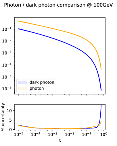
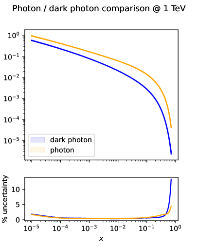
Figure 2.2: Comparison of $x\gamma(x,Q^{2})$ and $xB(x,Q^{2})$ at $Q=100\ \text{GeV}$ (left) and $Q=1\ \text{TeV}$ (right) for the values of dark photon mass and coupling given in Eq. (2.6). The percentage relative 68% C.L. PDF uncertainties of the photon and the dark photon are displayed in the bottom inset.

In Fig. 2.2, we display both the photon and dark photon PDFs in our representative dark set (obtained by setting the dark photon coupling and mass at the values given in Eq. (2.6)) at the scales $Q=100\ \text{GeV}$ and $Q=1\ \text{TeV}$, and show their relative PDF uncertainties. As anticipated, the dark photon PDF features the same functional form as the photon PDF (this is to be expected since the photon and dark photon splitting functions are identical up to scaling), but its density is smaller since $\alpha_{B}\lesssim\alpha$. Furthermore, it can be shown that increasing $\alpha_{B}$, and also moderately decreasing $m_{B}$, increases the similarity of the dark photon and photon PDFs. The dark photon uncertainty is mostly comparable to the photon uncertainty up to $x\sim 0.4$, and then increases faster than the photon uncertainty. This is due to the dark photon being generated off the singlet PDF (the sum of all quarks and antiquarks) at its mass threshold with a rather small coupling; in particular, the dark photon uncertainty is comparable to the uncertainty of the singlet PDF scaled by a factor of $\alpha_{B}$. This makes it comparable to the photon PDF uncertainty (for the choice of $\alpha_{B}$ and $m_{B}$ of Eq. (2.6)), except in the large-$x$ region where the singlet PDF uncertainty dramatically increases, resulting in the dark photon PDF uncertainty to consistently increase up to $\sim 10\%$ at $x\sim 0.6$. We have verified that for larger couplings the uncertainty increases, as one would expect.

Now that we have introduced a new parton in the proton, it is interesting to ask how much ‘space’ it takes up; this can be quantified by determining the momentum carried by the dark photon at different energy scales. As usual, the momentum fraction carried by any given parton flavour $f$ at the scale $Q$ is defined by:

$$\langle x\rangle_{f}(Q):=\int\limits_{0}^{1}dx\ xf(x,Q).$$ (2.7)

In Table. 2.1, we give a comparison between the momentum carried by the dark photon, the photon and the singlet for the representative dark PDF set computed using the values specified in Eq. (2.6), and compare them to the baseline SM PDF set, at $Q=100$ GeV and $Q=1$ TeV. We observe that the fraction of the proton momentum carried by the dark photon increases with the scale $Q$, which is to be expected by analogy with the photon’s behaviour. Depending on the coupling and the mass of the dark photon, the latter carries up to a fraction of percent of the proton momentum’s fraction at $Q\approx 1\ \text{TeV}$.

$\langle x\rangle_{f}(Q=100$ GeV)	$f=\Sigma$	$f=\gamma$	$f=B$
Baseline	50.23%	0.4241%	0%
Dark set	50.17%	0.4241%	0.03214%
$\langle x\rangle_{f}(Q=1$ TeV)	$f=\Sigma$	$f=\gamma$	$f=B$
Baseline	48.36%	0.5279%	0%
Dark set	48.12%	0.5275%	0.1357%

Table 2.1: A comparison between the momentum fraction percentage carried by the singlet $\Sigma$, the photon $\gamma$, and the dark photon $B$ at $Q=100$ GeV and $Q=1$ TeV, for the baseline SM set and the dark PDF set, obtained with the photon coupling and mass given in Eq. (2.6). The momentum fraction is computed on the central replica in each case.

Crucially, the presence of a dark photon in the DGLAP equations also modifies the evolution of all other flavours of PDFs due to the coupling of the PDFs via the modified DGLAP equations Eq. (2.1). We expect that the modification of the quark and antiquark flavours is strongest, as the dark photon is directly coupled to them. We also anticipate a modification to the gluon and photon PDFs, but these will be second order effects, so we expect that they will be smaller in comparison. Moreover, the density of each of the flavours should reduce, as the new dark photon ‘takes up space’ in the proton which was previously occupied by the other flavours.

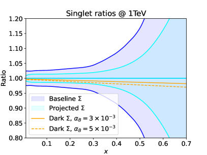
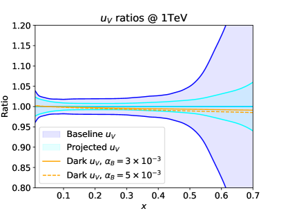
Figure 2.3: In solid orange, the ratio between the central singlet PDF $\Sigma$ (left) and central $u$-valence PDF (right), drawn from the dark benchmark scenario in Eq. (2.6), to the baseline SM central replica at $Q=1\ \text{TeV}$. In dashed orange, the same ratios but between the SM baseline and a dark PDF set produced using $m_{B}=50\ \text{GeV},\alpha_{B}=5\times 10^{-3}$. In each case, the uncertainty bands represent the 68% C.L. PDF uncertainties of the baseline set (in blue) and the projected PDF uncertainties at the HL-LHC, determined from Ref. Khalek:2018 (in light blue). The deviation when $\alpha_{B}=5\times 10^{-3}$ approaches the boundary of the projected HL-LHC uncertainty bands, consistent with the behaviour we see in Fig. 3.2 later; increasing $\alpha_{B}$ (and also to a milder extent, decreasing $m_{B}$) pushes the deviation outside of projected HL-LHC uncertainty bands. See the main text for more details.

Results are shown in Fig. 2.3, in which the ratio between the central value of the dark-photon modified singlet ($u$-valence) PDF and the central value of the baseline singlet ($u$-valence) PDF are displayed and compared to the current 68% C.L. PDF uncertainty.

We observe that the modification of the singlet becomes visible at about $x\sim 0.2$ and reaches 3% at larger values of $x\sim 0.5$. This is well within the 68% C.L. uncertainty of the singlet PDF from the baseline NNPDF3.1luxQED NNLO set. However, thanks to the inclusion of a vast number of new datasets and the increased precision of the methodology used in global PDF analysis, the recent NNPDF4.0 NNLO set Ball:2021leu displays significantly smaller large-$x$ uncertainty. Such a decrease in PDF uncertainties goes in the direction indicated by the dedicated study on how PDF uncertainties will decrease in future, thanks to the inclusion of precise HL-LHC measurements Khalek:2018 . In particular, to give an indication of how the modification of PDFs due to the presence of a dark photon might come into tension with decreasing PDF uncertainties during the HL-LHC phase, we display the projected 68% PDF uncertainties at the HL-LHC determined in the ‘optimistic’ scenario, Scenario 3, of Ref. Khalek:2018 . In this case, should PDF uncertainties decrease to the level predicted by Ref. Khalek:2018 , the distorted singlet PDF approaches the edge of the projected PDF uncertainty at $x\sim\,0.1-0.3$ region, for the values given in Eq. (2.6). This is particularly relevant for the analysis that we present in the next section.

3 Probing the Dark Sector

In this section we review the existing constraints on the dark photon. Subsequently, in order to assess the impact of a non-zero dark photon parton density on physical observables, we plot the parton luminosities when the dark photon is included, as compared to our baseline SM set. We compare the predicted deviations with the current PDF uncertainties and with the projected PDF uncertainties at the HL-LHC. Finally, we motivate and present our analysis of projected HL-LHC Drell-Yan data and compare the maximal sensitivity we can achieve to the existing bounds derived in the literature.

3.1 Review of existing constraints on the dark photon

To appreciate the utility of the dark photon PDF at colliders, we may compare to alternative probes. Recent works considering this class of baryonic dark photon models include Dobrescu:2014fca ; Dror:2017ehi ; Ismail:2017fgq ; Dror:2018wfl ; Ilten:2018crw ; Dobrescu:2021vak . There are a variety of competing constraints on this scenario, of varying theoretical robustness.

One class of constraints, first considered in detail in Dobrescu:2014fca , is theoretical and concerns the mixed $\text{U}(1)_{B}-$EW anomalies. Suppose we envisage that the UV-completion of the model Eq. (2.6) is perturbative with $\text{U}(1)_{B}$ linearly realised. In that case the mixed anomaly must be UV-completed by some fermions with electroweak charges. In this perturbative UV-completion they will obtain their mass from spontaneous $\text{U}(1)_{B}$-breaking. As a result, they will be coupled to the longitudinal mode of $B$ and an additional Higgs-like scalar with a Yukawa coupling $\lambda\propto M_{F}/v_{B}$, where $M_{F}$ is the fermion mass, $v_{B}$ is the $\text{U}(1)_{B}$-breaking expectation value, and we have assumed three sets of fermions with the same charge ($1/3$) as the left-handed fermions, for simplicity. On the other hand we have $g_{B}\propto M_{B}/v_{B}$ following from the charge and symmetry-breaking vacuum expectation value. As a result, we expect:

$$g_{B}\approx\frac{2\lambda}{3}\frac{M_{B}}{M_{F}}~{}~{},$$ (3.1)

where the precise numerical factors are taken from Dobrescu:2014fca . Thus, requiring perturbativity $\lambda\lesssim 4\pi$ implies an upper bound on $g_{B}$, where the factor $1/3$ follows from the fact that each family of fermions is in triplicate to mirror the QCD multiplicity of the SM quarks. This limit is shown as a dashed line in Fig. 3.4 where we have taken $M_{F}\geq 90$ GeV for the electroweak-charged fermions.

However, a number of implicit assumptions have been made which can weaken upon further inspection. To see this, consider cancelling the anomaly with $N$ copies of the above class of fermions. In this case the limit becomes:

$$g_{B}\lesssim\frac{8\pi}{3}\frac{N}{3}\frac{M_{B}}{M_{F}}~{}~{}.$$ (3.2)

Hence we see that this theoretical limit makes not only the assumption of a weakly-coupled UV-completion, but also depends on assumptions of minimality of the UV completion as well. As a result, while this limit does guide the eye as to the nature of the UV-completion, it cannot be considered a strong theoretical limit on the model parameters.

The only truly model-independent theoretical limit comes from considering the scale at which the validity of the IR theory itself breaks down. Given that the quark interactions are vector-like there is no possibility of tree-level unitarity violation in quark scattering mediated by $B$, thus we must look to quantum effects. In this case the mixed-anomaly becomes relevant and renders the theory non-unitary unless Preskill:1990fr :

$$g_{B}\lesssim\frac{(4\pi)^{2}}{3\alpha_{W}}\frac{M_{B}}{M_{\Lambda}}~{}~{},$$ (3.3)

where $\alpha_{W}$ is the $\text{SU}(2)$ fine structure constant at the electroweak scale and $M_{\Lambda}$ is the energy scale at which the theory becomes strongly coupled. Numerically this is

$$g_{B}\lesssim\frac{3M_{B}}{5\text{ GeV}}\frac{10\text{ TeV}}{M_{\Lambda}}~{}~{},$$ (3.4)

which is too weak to be relevant for our purposes. As a result we conclude that the effective theory considered here is valid throughout the energy scales under investigation. However, we note that, as shown in Dobrescu:2021vak , the mixing with the $Z$-boson is sensitive to the details of the UV-completion; for this reason we restrict the mass range under investigation to $m_{B}\leq 80\ \text{GeV}$, above which these UV-dependent effects can be important.

There are three relevant classes of experimental constraints. The first concerns the exotic $Z$-boson decays $Z\to B\gamma$. These constraints were calculated in Dror:2017ehi based on the LEP analysis for $Z\to H\gamma$, $H\to$hadrons L3:1996dmt . This limit, relevant to the higher mass range, is shown in red in Fig. 3.4. The second class of constraints at lower masses concerns exotic $\Upsilon$ decays Carone:1994aa ; Aranda:1998fr , where the constraint is dominated by limits on $\Upsilon(1S)\to 2$ jets ARGUS:1986nzm , shown in blue in Fig. 3.4. Finally, there are additional searches for hadronically decaying resonances at hadron colliders Dobrescu:2013cmh ; Shimmin:2016vlc ; ATLAS:2019itm ; Dobrescu:2021vak . The strongest are from CMS $B+$ISR searches CMS:2019xai ; CMS:2019emo , shown in yellow in Fig. 3.4.

3.2 Effects of the dark photon on parton luminosities

In Sec. 2, we showed that the presence of a dark photon modifies all other flavours of PDFs via the mixing associated with the DGLAP evolution equations, with a modification that is proportional to $\alpha_{B}$ and the logarithm of $m_{B}$. In order to assess the impact of a dark photon parton density on physical observables, and thus extract the sensitivity that the LHC can achieve on the parameters of the model, in the following subsection we compare the size of the dark parton luminosities to luminosities involving the other partons, and assess the impact of the dark photon on the dominant partonic channels.

Parton luminosities are doubly differential quantities defined as:

$$\frac{d{\cal L}_{ij}}{dyd\tau}=f_{i}(x_{1},Q)f_{j}(x_{2},Q)\qquad x_{1,2}=\sqrt{\tau}\exp(\pm y)\qquad\tau=\frac{M_{X}^{2}}{S},$$ (3.5)

where $S$ is the squared centre-of-mass energy of the hadronic collision, $M_{X}$ is the invariant mass of the partonic final state, $y$ is the rapidity of the partonic final state, and $f_{i}(x,Q)$ is the PDF of the $i^{\rm th}$ parton evaluated at the scale $Q$. Different choices for $Q$ can be adopted in order to improve predictions of a particular process and/or distribution. At the level of pure luminosities, without the convolution with any specific matrix element, the factorisation scale can be naturally set to $Q=M_{X}$. For plotting purposes, it is useful to define the $M_{X}$-differential luminosities, given by:

$$\Phi_{ij}(M_{X})\,=\,\frac{d{\cal L}_{ij}}{dM_{X}^{2}}=\frac{1}{S}\,\int\limits_{M_{X}^{2}/S}^{1}\frac{dx}{x}\ f_{i}(x,M_{X})f_{j}\left(\frac{M_{X}^{2}}{xS},M_{X}\right).$$ (3.6)

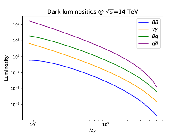
Figure 3.1: Comparison of the absolute value of the $\Phi_{BB}$, $\Phi_{qB}$ central luminosities and the $\Phi_{\gamma\gamma}$ and $\Phi_{qq}$ central luminosities as a function of the invariant mass $M_{X}$ at the centre of mass energy $\sqrt{s}=14\ \text{TeV}$ for the dark PDF set obtained with the dark photon coupling and mass set in Eq. (2.6).

We first compare the size and the $M_{X}$-dependence of the different parton luminosities in the candidate dark PDF set obtained by setting the mass and the coupling to the values indicated in Eq. (2.6). In Fig. 3.1 we plot $\Phi_{BB},\Phi_{Bq}$ as compared to $\Phi_{q\bar{q}}$, $\Phi_{\gamma\gamma}$. We observe that, while the $BB$ channel is suppressed by two powers of the dark coupling, and its size never exceeds more than a fraction of a percent of the $q\bar{q}$ luminosity, the $Bq$ channel grows from about 2% of the $q\bar{q}$ luminosity at $M_{X}\sim$ 1 TeV to about 8% of the $q\bar{q}$ luminosity at larger values of the invariant mass. Its contribution exceeds that of $\gamma\gamma$ scattering by one order of magnitude.

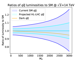
(a) $m_{B}=50\ \text{GeV},\alpha_{B}=3\times 10^{-3}$

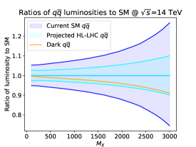
(b) $m_{B}=50\ \text{GeV},\alpha_{B}=5\times 10^{-3}$

(c) $m_{B}=5\ \text{GeV},\alpha_{B}=3\times 10^{-3}$

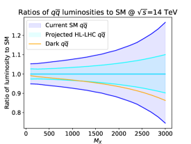
(d) $m_{B}=5\ \text{GeV},\alpha_{B}=5\times 10^{-3}$

Figure 3.2: The ratio $\Phi_{q\bar{q}}^{\text{Dark}}/\Phi_{q\bar{q}}^{\text{SM}}$ for the total quark-anti-quark luminosity, at the centre of mass energy $\sqrt{S}=14\ \text{TeV}$ for the values of mass and coupling indicated under each panel. In each panel, the dark blue bands correspond to the current PDF uncertainty, while the light blue bands show the expected uncertainty on the PDF luminosity at the HL-LHC. See main text for more details.

We now turn to assess the change in the other luminosities, as a result of the inclusion of a non-zero dark photon parton density. In Fig. 3.2 we display the ratio of the dark-photon modified quark-antiquark integrated luminosity $\Phi_{q\bar{q}}^{\text{Dark}}$ with the baseline one, $\Phi_{q\bar{q}}^{\text{SM}}$ at the centre of mass energy $\sqrt{S}=14\ \text{TeV}$, for different values of the $\alpha_{B}$ and $m_{B}$ parameters, starting from our benchmark values, Eq. (2.6). In each figure, the dark blue band corresponds the 68% C.L. PDF uncertainty of the NNLO baseline NNPDF3.1luxQED set, while the green bands show the projected PDF uncertainty on the parton luminosity at the HL-LHC; this estimate for the uncertainty on the PDF luminosity is obtained from the ‘optimistic’ scenario, Scenario 3, analysed in Khalek:2018 , as above. Starting from the values of Eq. (2.6), we observe that the deviation in the $q\bar{q}$ luminosity due to the presence of the dark photon is significant compared to the size of the projected PDF uncertainties at the HL-LHC. Decreasing the mass of the dark photon by a factor of 10 increases the impact of the dark photon on $q\bar{q}$ initiated observables, while increasing the coupling by less than a factor of 2 brings the luminosity beyond the edge of the 68% C.L. error bands.

Crucially, the effect of the dark photon is much larger in the $q\bar{q}$-initiated processes than in any of the other channels, including $qq$, $qg$ and $gg$. This motivates the study of the high-mass Drell-Yan tails that we put forward in the following section.

3.3 Constraints from precise measurements of high-energy Drell-Yan tails

Given that the $q\bar{q}$ channel is the most affected by the presence of a non-zero dark photon parton density, in this study we focus on precise measurements of the high-mass Drell-Yan tails at the HL-LHC. It is important to note that these projected data are not included in the fit of the input PDF set used as a baseline, otherwise, as was explicitly shown in  Carrazza:2019sec ; greljo_parton_2021 ; Iranipour:2022iak , the interplay between the fit of the new physics parameters and the fit of the PDF parametrisation at the initial scale might distort the results.

To generate the HL-LHC pseudodata for neutral-current high-mass Drell-Yan cross sections at $\sqrt{S}=14$ TeV, we follow the procedure of greljo_parton_2021 . Namely, we adopt as reference the CMS measurement at 13 TeV CMS:2018mdl based on $\mathcal{L}=2.8$ fb^-1. The dilepton invariant mass distribution $m_{\ell\ell}$ is evaluated using the same selection and acceptance cuts of CMS:2018mdl , but now with an extended binning in $m_{\ell\ell}$ to account for the increase in luminosity. We assume equal cuts for electrons and muons, and impose $|\eta_{\ell}|\leq 2.4$, $p_{T}^{\rm lead}\geq 20$ GeV, and $p_{T}^{\rm sublead}\geq 15$ GeV for the two leading charged leptons of the event. We restrict ourselves to events with $m_{\ell\ell}$ greater than $500$ GeV, so that the total experimental uncertainty is not limited by our modelling of the expected systematic errors, by making our projections unreliable. To choose the binning, we require that the expected number of events per bin is bigger than 30 to ensure the applicability of Gaussian statistics. Taking into account these considerations, our choice of binning for the $m_{\ell\ell}$ distributions at the HL-LHC both in the muon and electron channels are displayed in Fig. 3.3 with the highest energy bins reaching $m_{\ell\ell}\simeq 4$ TeV. In total, we have two invariant mass distributions of 12 bins each, one in the electron and one in the muon channels.

Concerning uncertainties, in  greljo_parton_2021 this data is produced by assuming that the HL-LHC phase will operate with a total integrated luminosity of $\mathcal{L}=6\ \text{ab}^{-1}$ (from the combination of ATLAS and CMS, which provide ${\cal L}=3\,{\rm ab}^{-1}$ each), and also assuming a five-fold reduction in systematic uncertainty compared to  CMS:2018mdl . We regard this scenario as optimistic in this paper; we also manipulated the projected data so that it reflected a more conservative possibility, where the total integrated luminosity of the high-mass Drell-Yan tail measurements is $\mathcal{L}=3\ \text{ab}^{-1}$ (say, for example, they are made available only by either ATLAS or CMS) and with a two-fold (rather than a five-fold) reduction in systematic uncertainties.

For these projections, the reference theory is the SM, with theoretical predictions evaluated at NNLO in QCD including full NLO EW corrections (including in particular the photon-initiated contributions); note, however, that the Drell-Yan production has been recently computed at N³LO in QCD Duhr:2020seh ; Duhr:2021vwj . In the kinematical region that is explored by our HL-LHC projections ($m_{\ell\ell}>500$ GeV), the perturbative convergence of the series is good and the N³LO computation is included within the NNLO prediction, with missing higher order uncertainty going from about 1% to a fraction of a percent. Given the good perturbative convergence of the matrix element calculation, and the absence of N³LO PDFs that match the accuracy of the N³LO computation of the matrix element, we use the NNLO QCD and NLO EW accuracy of our calculations, both for the SM baseline and for the dark-photon modified PDF set that we use to compute the maximal sensitivity to the dark photon parameters.

The central PDF set used as an input to generate the theoretical prediction is the SM baseline that we use throughout the paper, namely the NNLO NNPDF3.1luxQED set. The central values for the HL-LHC pseudodata are then generated by fluctuating the reference theory prediction by the expected total experimental uncertainty, namely

$$\sigma^{\rm hllhc}_{i}\equiv\sigma^{\rm th}_{i}\left(1+\lambda\delta_{\cal L}^{\rm exp}+r_{i}\delta_{{\rm tot},i}^{\rm exp}\right)\,,\qquad i=1,\ldots,n_{\rm bin}\,,$$ (3.7)

where $\lambda,r_{i}$ are univariate Gaussian random numbers, $\delta_{{\rm tot},i}^{\rm exp}$ is the total (relative) experimental uncertainty corresponding to this specific bin (excluding the luminosity and normalisation uncertainties), and $\delta_{\cal L}^{\rm exp}$ is the luminosity uncertainty, which is fully correlated amongst all the pseudodata bins of the same experiment. We take this luminosity uncertainty to be $\delta_{\cal L}^{\rm exp}=1.5$% for both ATLAS and CMS, as done in Khalek:2018 .

To obtain bounds on the dark photon mass and coupling, we select a grid of benchmark points $(m_{B},\alpha_{B})$ in the dark photon parameter space; our scan consists of $21$ points, distributed as a rectangular grid with masses $m_{B}=2,5,8,10,20,50,80\ \text{GeV}$ and couplings $\alpha_{B}=10^{-3},2\times 10^{-3},3\times 10^{-3}$. We then construct dark PDF sets at each of these benchmark points (thus a total of $21$ PDF sets, in each case including quarks, antiquarks, the gluon, the photon and the dark photon PDFs), using the appropriate values of $m_{B},\alpha_{B}$, and hence compute theoretical predictions in both the optimistic and conservative scenarios at each grid point. The predictions are produced assuming that the primary contribution comes from the $q\bar{q}$ channel; in particular, we note that the partonic diagrams that include a dark photon in the initial state (such as $Bq\to\bar{q}l^{+}l^{-}$ or $B\bar{q}\to ql^{+}l^{-}$) are suppressed by two powers of $\alpha_{B}$, one from the dark photon PDF and one from the matrix element, and therefore are suppressed beyond the accuracy of our calculation.

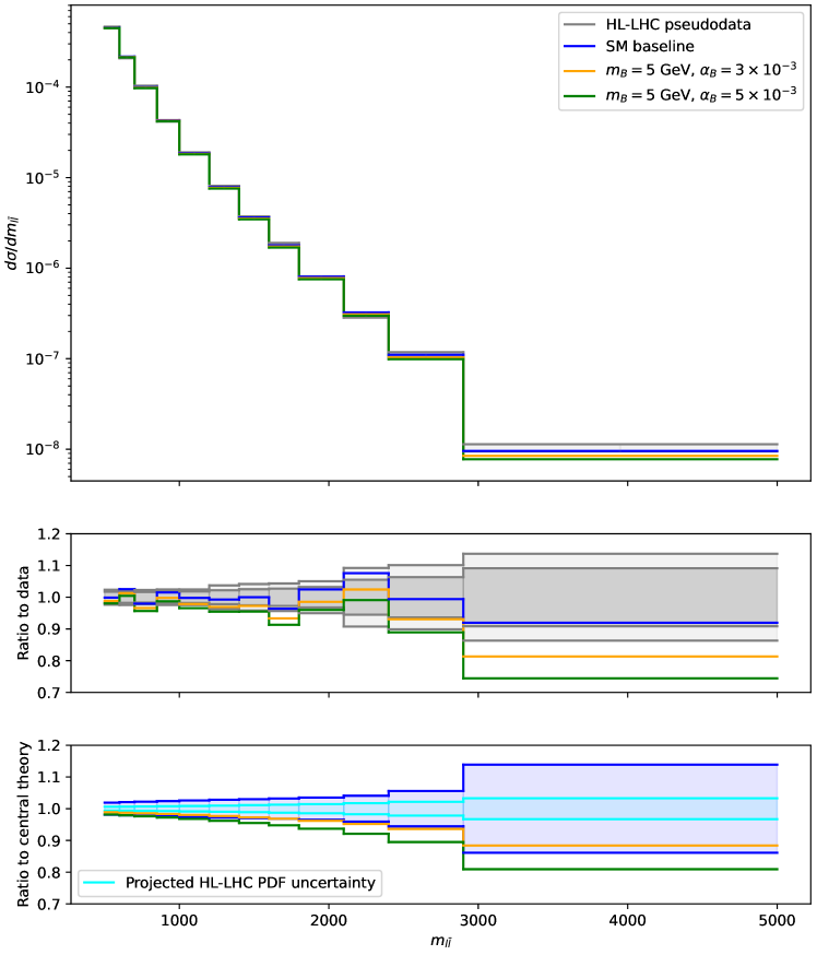
Figure 3.3: Top: data-theory comparison between HL-LHC pseudodata in the electron channel generated according to Eq. (3.7) (grey, with optimistic uncertainties displayed), and the theoretical predictions obtained using the NNLO baseline PDF set NNPDF3.1luxQED (blue) and those obtained using the dark PDF sets produced with parameters $(m_{B},\alpha_{B})=(5\ \text{GeV},3\times 10^{-3}),(5\ \text{GeV},5\times 10^{-3})$ (yellow, green respectively). Middle: ratio of the baseline SM central predictions obtained using the baseline, and the central predictions obtained using the two representative dark PDF sets, to the central values of the pseudodata. The relative experimental uncertainties in both the optimistic scenario (dark grey) and conservative scenario (light grey) are displayed. Bottom: ratio of the central predictions obtained using the two representative dark PDF sets to the baseline SM central predictions, with both the PDF uncertainty from the baseline PDF set (dark blue) and the projected PDF uncertainty at the HL-LHC in the optimistic scenario of  Khalek:2018 (light blue) displayed.

In Fig. 3.3 we display the data-theory comparison between the HL-LHC pseudodata in the electron channel, generated according to Eq. (3.7), and both the SM theoretical predictions obtained using the NNLO baseline PDF set NNPDF3.1luxQED and the predictions obtained using the dark PDF sets produced with the dark photon mass and coupling set to $(m_{B}=5\,{\rm GeV},\alpha_{B}=3\times 10^{-3})$ and $(m_{B}=5\,{\rm GeV},\alpha_{B}=5\times 10^{-3})$ respectively. We also display the ratio between the central values of those predictions and the central values of the pseudodata as compared to their relative experimental uncertainty in both the optimistic and conservative scenarios. We see that whilst the SM predictions are within the $1\sigma$ experimental uncertainty (by construction), the dark-photon modified predictions display significant deviations. In the bottom inset we show the ratio between the predictions obtained in the two representative dark photon scenarios to the central SM theoretical predictions obtained with the the baseline SM PDF set. PDF uncertainties are shown; we display both the current PDF uncertainty of the NNLO baseline PDF set NNPDF3.1luxQED and the projected PDF uncertainties at the HL-LHC, obtained as described at the beginning of this section. Comparing the size of the PDF uncertainties to the size of the projected experimental uncertainties at the HL-LHC, we observe that whilst the current PDF uncertainties are comparable to the experimental uncertainties of the projected data, the projected HL-LHC uncertainties are subdominant as compared to the experimental uncertainties of the pseudodata.

The $\chi^{2}$-statistic of the resulting dark PDF set’s predictions on high-luminosity high-mass neutral-current DY data is defined as:

$$\chi^{2}(m_{B},\alpha_{B}):=||\textbf{T}(m_{B},\alpha_{B})-\textbf{D}||^{2}_{\Sigma^{-1}},$$ (3.8)

where $||\textbf{v}||_{A}^{2}=\textbf{v}^{T}A\textbf{v}$, D is the projected data, $\textbf{T}(m_{B},\alpha_{B})$ are the theoretical predictions using a dark PDF set containing a dark photon of mass $m_{B}$ and coupling $\alpha_{B}$, and $\Sigma$ is the total covariance matrix (incorporating both experimental and theoretical uncertainties):

$$\Sigma=\Sigma^{\rm th}+\Sigma^{\rm exp}.$$ (3.9)

From Fig. 3.3 we observe that, depending on the assumption we make on PDF uncertainties in the HL-LHC era, it may be important to include the PDF uncertainties in the theory covariance matrix, while the component of the theory covariance matrix associated with the scale uncertainty of the NNLO computation is subdominant. Of course, it would be unrealistic to assume that the PDF uncertainty will not decrease as compared to the uncertainty of the NNPDF3.1luxQED baseline, given that we already know that in the updated NNPDF4.0 set Ball:2021leu the uncertainty of the large-$x$ quarks and antiquarks has already decreased by a sizeable amount thanks to the inclusion of precise LHC data. We thus decide to use the projected PDF uncertainties determined in Khalek:2018 ; in particular, we use Scenario 1 of  Khalek:2018 (the conservative scenario) when we consider the conservative experimental scenario, and we use Scenario 3 of  Khalek:2018 (the most optimistic scenario) when we consider the optimistic experimental scenario. In Appendix C we discuss how our results depend on the assumptions we make on PDF uncertainties. Assuming that the projected PDF uncertainties at the HL-LHC that we display in the bottom inset of Fig. 3.3 are realistic, even in the most optimistic scenario they still amount to 4% to 6% in the largest bins. Therefore, their contribution is much larger than the scale uncertainty of the Drell-Yan matrix element at NNLO in QCD; hence PDF uncertainty is the dominant theory uncertainty on the predictions, and thus it is this contribution that is included in the theory covariance matrix.

To compute the contribution of PDF uncertainties to the theory covariance matrix, we build the theoretical covariance as defined in Hartland:2019bjb :

$$\Sigma^{\rm th}_{ij}=\langle d\sigma_{i}^{{\rm th},(r)}d\sigma_{j}^{{\rm th},(r)}\rangle_{\rm rep}-\langle d\sigma_{i}^{{\rm th},(r)}\rangle_{\rm rep}\langle d\sigma_{j}^{{\rm th},(r)}\rangle_{\rm rep},$$ (3.10)

where the theoretical predictions for the differential cross section $d\sigma_{i}^{{\rm th},(r)}$ are computed using the SM theory and the $r^{\rm th}$ replica from the baseline PDF set, with PDF uncertainties rescaled by the HL-LHC uncertainty reduction, and averages $\langle\cdot\rangle_{\rm rep}$ are performed over the $N_{\rm rep}=100$ replicas of this PDF set.

We define the difference in $\chi^{2}$ to be:

$$\Delta\chi^{2}(m_{B},\alpha_{B}):=\chi^{2}(m_{B},\alpha_{B})-\chi^{2}_{0},$$ (3.11)

where $\chi^{2}_{0}$ is the $\chi^{2}$-statistic when predictions from the baseline set are used instead. For each fixed $m_{B}=m_{B}^{*}$ in the scan, we then model $\Delta\chi^{2}(m_{B}^{*},\alpha_{B})$ as a quadratic in $\alpha_{B}$ and determine the point at which $\Delta\chi^{2}=3.8$, corresponding to a confidence of 95% in a one-parameter scan. Hence, we construct 95% confidence bounds on $m_{B},\alpha_{B}$ (and hence $m_{B},g_{B}$ via an appropriate conversion) as displayed in Fig. 3.4. There, the purple (dashed) projected bounds are computed in the conservative scenario excluding (including) the PDF theory covariance matrix, and the green (dashed) projected bounds are computed in the optimistic scenario excluding (including) the PDF theory covariance matrix.

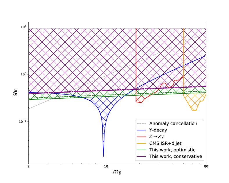
Figure 3.4: Comparison of the projected HL-LHC sensitivity computed in this work in the optimistic (green) and conservative (purple) scenarios with the existing bounds described in Sec. 3.1. The solid green and purple lines correspond to projected bounds obtained excluding projected PDF uncertainty, whilst the dashed lines correspond to projected bounds obtained including projected PDF uncertainty, as discussed in the text.

We observe that the projected HL-LHC sensitivity to the detection of a dark photon is competitive with existing experimental bounds, across a large range of possible masses, especially $m_{B}\in[2,6]\cup[25,50]\ \text{GeV}$. Even in the most conservative scenario including PDF uncertainty (shown as a dashed purple line), the projected sensitivity remains competitive with experiment. Furthermore, one of the useful features of our projected sensitivity is that it is uniformly excluding across a large range (because of the logarithmic dependence on $m_{B}$); when compared to individual bounds one at a time, for example the $\Upsilon$-decay bounds, or the anomaly bounds, our projected sensitivity is powerful.

4 Conclusions

While the dark sector has evaded a non-gravitational detection for decades it is possible that the first clues may be right under our noses, hidden in the dark depths of the proton. To illustrate this point we have considered the possible existence of a baryonic dark photon. Being coupled to quarks it may, through radiative effects, be present in the proton and carry some fraction of its momentum at colliders. In this work we have explicitly calculated the dark photon PDF and hence the dark parton luminosities at the LHC at leading order in the dark photon coupling.

Since any momentum fraction carried by the dark photon is not carried by the SM partons, the leading effect of the dark photon is to take away part of their momentum. Importantly, this affects precision predictions for event distributions at colliders. Being a high-precision observable at hadron colliders, DY production at high energies is sensitive to the dark photon content of the proton, through the reduction in light quark PDFs. To this end, we have shown that future DY measurements at the HL-LHC are competitive with present lower energy probes in constraining regions of dark photon parameter space. This reveals a new facet of the era of precision hadron collider physics we are currently entering.

Of course our projected sensitivity is based on the phenomenology tools that we currently have, while the actual analysis of real data at the HL-LHC will be able to use the tools that will be developed by then. Most importantly new global PDF sets will be made available, which will possibly be done at N³LO, and resulting PDFs can be consistently used with N³LO computations of the matrix elements. Moreover the associated PDF uncertainty will most certainly include a missing higher order uncertainty component in the PDF uncertainty that is not currently included in any of the global NNLO PDF fits. The actual sensitivity calculated with real data at the HL-LHC and the refined tools that the PDF community is working towards will be compared with the analysis we have put forward in this work, and the power of the LHC in constraining or revealing the presence of a dark photon will be unveiled.

It is widely accepted that we must endeavour to search in every corner of parameter space for evidence of the dark sector. This has led to a blossoming of novel theoretical ideas and ingenious experimental advances as an ever-greater range of viable dark sector possibilities come under scrutiny. At the same it is important to reflect on our limited view of the dark sector and, perhaps, look inwards. In this work we have pursued this strategy in a very literal sense, asking “Could dark sector constituents lie within the baryons that make up the visible world?” Our results suggest that they could, leaving their fingerprints in SM processes at the HL-LHC.

Appendix A Calculation of the dark photon splitting functions

In this Appendix, we explicitly compute the leading order dark photon splitting functions.

We begin by reminding the reader of one possible definition of leading order splitting functions. Consider a process initiated by some parton, which has the potential to radiate another parton before participating in a hard reaction (either a virtual parton, which is reabsorbed, or a real parton which is emitted). Suppose that radiation occurs via a vertex with coupling $g$ (which could be taken to be $g_{s}$, $e$ or $g_{B}$, the strong, electric, or dark couplings as appropriate), and corresponding fine structure constant $\alpha=g^{2}/4\pi$. The cross-section for the radiative process can be shown to take the form:

$$\sigma^{\text{NLO}}=\frac{\alpha}{2\pi}\int\frac{d(|\textbf{l}_{T}|^{2})}{|\textbf{l}_{T}|^{2}}\int\limits_{0}^{1}dx\ P(x)\sigma^{\text{Born}}(xp)+\text{terms that are finite as $\textbf{l}_{T}\rightarrow 0$}.$$ (A.1)

Here, $\sigma^{\text{Born}}(xp)$ is the cross-section when parton radiation does not occur, $\textbf{l}_{T}$ is the transverse momentum of the radiated parton and $x$ is the fraction of momentum of the parton that goes on to take part in the hard reaction. The factor $P(x)$ is called the splitting function and depends on the type of parton initiating the process, the type of parton radiated, and the type of parton that goes on to participate in the hard reaction; typically it is written $P_{ij}(x)$ where $i$ is the parton which goes on to participate in the hard reaction, $j$ is the initial parton, and the third parton flavour is left implied by the structure of the theory. In particular, we see that it multiplies the most collinearly divergent part of the integrand on the right hand side of Eq. (A.1).

We now explicitly compute the splitting functions for each of the four dark photon splitting channels, shown in Fig. 2.1.

Contribution to $P_{qq}^{(0,0,1)}(x)$

Consider a general leading order partonic process where a quark $q$ scatters off another particle $k$ to produce some final state $X$ via some hard interaction, as shown in Fig. A.1.

Figure A.1: Feynman diagram corresponding to a Born-level quark-initiated hard process.

The amplitude for this process can be written as $\mathcal{M}(p)u(p)$, where $\mathcal{M}(p)$ is the amplitude for the unknown hard scattering part of the diagram (taking as an argument the four-momentum $p$ of our incoming quark $q$), including the final state $X$ and the target particle $k$, and $u(p)$ is the appropriate plane-wave spinor coming from the initial quark $q$. After summing over all spins the amplitude gives rise to a cross-section:

$$\sigma^{\text{Born}}(p)=\frac{1}{4s}\sum_{X}\mathcal{M}(p)\not{p}\mathcal{M}^{\dagger}(p),$$ (A.2)

where the sum over $X$ includes an integral over the phase space of the final state $X$.

On the other hand, the initial quark $q$ may also radiate a real dark photon before it participates in the interaction. Such a contribution arises from the diagram shown in Fig. A.2.

Figure A.2: Feynman diagram corresponding to real radiation of a dark photon.

Let $l$ be the momentum of the outgoing dark photon. Then the amplitude for this diagram is:

$$\mathcal{M}(p-l)\frac{i}{\not{p}-\not{l}}\left(-\frac{ig_{B}}{3}\right)\not{\epsilon}(l)u(p)=\frac{g_{B}}{3(p-l)^{2}}\mathcal{M}(p-l)(\not{p}-\not{l})\not{\epsilon}(l)u(p),$$ (A.3)

where $\mathcal{M}(p-l)$ is the same amplitude for the hard subgraph above, but this time with momentum $p-l$ entering the graph. $\epsilon(p)$ denotes the polarisation of the dark photon.

In order to compute the splitting function contribution $P_{qq}^{(0,0,1)}(x)$, we must determine the most collinearly-divergent part of the amplitude of Eq. (A.3). To this end, we write $l$ in terms of its Sudakov decomposition:

$$l=(1-x)p+l_{T}+\frac{|\textbf{l}_{T}|^{2}}{1-x}\eta,$$ (A.4)

where $l_{T}$ is some transverse four-vector, $\eta$ is a null vector satisfying $2\eta\cdot p=1$, and $x$ is a constant chosen to make the decomposition true. In particular, we see that as $l_{T}\rightarrow 0$, we have $l\rightarrow(1-x)p$, i.e. the initial and radiated partons become collinear, and the parton which goes on to participate in the hard interaction has momentum fraction $x$. Therefore, in this notation, the collinear limit is $l_{T}\rightarrow 0$.

We now write Eq. (A.3) in terms of $l_{T}$, and hence determine the most collinearly divergent parts that we are required to retain. Via a short calculation, we can obtain:

$$-\frac{g_{B}(1-x)}{3|\textbf{l}_{T}|^{2}}\mathcal{M}(p-l)\left(x\not{p}-\not{l}_{T}-\frac{|\textbf{l}_{T}|^{2}}{1-x}\not{\eta}\right)\not{\epsilon}(l)u(p).$$ (A.5)

Retaining only the divergent terms as $l_{T}\rightarrow 0$, the modulus-squared spin-sum/averaged amplitude is then given by:

$$\frac{g_{B}^{2}}{9|\textbf{l}_{T}|^{2}}\left(\frac{1+x^{2}}{x}\right)\mathcal{M}(xp)x\not{p}\mathcal{M}^{\dagger}(xp).$$ (A.6)

Inserting into the standard cross-section formula, and appropriately changing integration variables, reveals that the most collinearly-divergent part of the cross-section associated to this process is given by:

$$\sigma^{\text{NLO,real}}(p)=\frac{\alpha_{B}}{2\pi}\int\frac{d(|\textbf{l}_{T}|^{2})}{|\textbf{l}_{T}|^{2}}\int\limits_{0}^{1}dx\ \frac{1}{9}\left(\frac{1+x^{2}}{1-x}\right)\sigma^{\text{Born}}(xp),$$ (A.7)

As it stands, we see that $\sigma^{\text{NLO,real}}(p)$ also contains a soft divergence as $x\rightarrow 1$, which characterises the divergence that occurs when the radiated parton’s energy tends to zero. The soft divergent part is cancelled by adding up the virtual contribution, which corresponds to a dark photon being emitted by the quark, and later being reabsorbed.

Fortunately, there is a clever probability argument which sidesteps actual computation of the virtual corrections. Let’s begin by writing the virtual corrections as:

$$\sigma^{\text{NLO,virtual}}(p)=A\sigma^{\text{Born}}(p),$$ (A.8)

where $A$ is some appropriately chosen constant. It follows that the sum of the virtual corrections and the leading order graph is given by $(1+A)\sigma^{\text{Born}}(p)$. Thus adding the virtual corrections, leading order graph and the real emission graph, we have:

$$\sigma^{\text{total}}(p)=\int\limits_{0}^{1}dx\left(\frac{1}{9}\left(\frac{1+x^{2}}{1-x}\right)+(1+A)\delta(1-x)\right)\sigma^{\text{Born}}(xp).$$ (A.9)

We interpret the coefficient of $\sigma^{\text{Born}}(xp)$ as the possible outcomes for the initial quark: it either radiates a $B$-boson, radiates a virtual quark which later recombines with the original quark, or it does none of the above. At this order, these are the only possibilities, and hence the probabilities of these events must sum to $1$:

$$\int\limits_{0}^{1}dx\left(\frac{1}{9}\left(\frac{1+x^{2}}{1-x}\right)\Theta(1-\epsilon-x)+(1+A)\delta(1-x)\right)=1.$$ (A.10)

where we introduce the regulator $\epsilon$ that cuts off the integral at $1-\epsilon$ by using the Heaviside step function $\Theta$. We can now compute the (divergent) value of $A$ that enforces this condition, finding:

$$A=\frac{1}{6}+\frac{2}{9}\log(\epsilon).$$ (A.11)

This reveals that the splitting function can be written (in a distributional sense) as:

$$P_{qq}^{(0,0,1)}(x)=\lim_{\epsilon\rightarrow 0}\left[\frac{1}{9}\left(\frac{1+x^{2}}{1-x}\right)\Theta(1-\epsilon-x)+\left(\frac{1}{6}+\frac{2}{9}\log(\epsilon)\right)\delta(1-x)\right].$$ (A.12)

Manipulating this distribution shows that $P_{qq}^{(0,0,1)}(x)$ can be written in the more concise form:

$$P_{qq}^{(0,0,1)}(x)=\frac{1+x^{2}}{9(1-x)_{+}}+\frac{1}{6}\delta(1-x),$$ (A.13)

where the plus distribution is defined in Eq. (2.5).

Contribution to $P_{qB}^{(0,0,1)}(x)$

In order to work out the contribution to $P_{qB}^{(0,0,1)}(x)$, we consider the radiation of an antiquark from a dark photon, as shown in Fig. A.3.

Figure A.3: Feynman diagram corresponding to real radiation of an antiquark.

The amplitude for this diagram is given by:

$$\frac{g_{B}}{3(p-l)^{2}}\mathcal{M}(p-l)(\not{p}-\not{l})\not{\epsilon}(p)v(l).$$ (A.14)

As before, we can use the Sudakov decomposition to write the amplitude in terms of the transverse momentum $l_{T}$:

$$-\frac{g_{B}(1-x)}{3|\textbf{l}_{T}|^{2}}\mathcal{M}(xp)(x\not{p}-\not{l}_{T})\not{\epsilon}(p)v(l),$$ (A.15)

where we drop all terms that remain finite as $l_{T}\rightarrow 0$. Further simplification of the spinor structure, and ignoring terms that remain finite as $l_{T}\rightarrow 0$ throughout, the modulus-squared spin-sum/averaged amplitude becomes:

$$\frac{g_{B}^{2}(1-x)}{9|\textbf{l}_{T}|^{2}}\left(\frac{2x^{2}-2x+1}{x}\right)\mathcal{M}(xp)x\not{p}\mathcal{M}^{\dagger}(xp).$$ (A.16)

Inserting into the cross-section formula, we have:

$$\sigma^{\text{NLO}}(p)=\frac{\alpha_{B}}{2\pi}\int\frac{d(|\textbf{l}_{T}|^{2})}{|\textbf{l}_{T}|^{2}}\int\limits_{0}^{1}dx\ \left(\frac{2x^{2}-2x+1}{9}\right)\sigma^{\text{Born}}(xp).$$ (A.17)

and hence we deduce that the splitting function is given by:

$$P_{qB}^{(0,0,1)}(x)=\frac{2x^{2}-2x+1}{9}=\frac{(1-x)^{2}+x^{2}}{9}.$$ (A.18)

In this case, there are no virtual corrections to take care of at this order.

Contribution to $P_{BB}^{(0,0,1)}(x)$

Having found $P_{qB}^{(0,0,1)}(x)$, it is straightforward to find $P_{BB}^{(0,0,1)}(x)$ using the fact that probabilities must sum to $1$. At this order, the only contribution to $P_{BB}^{(0,0,1)}(x)$ is given by a virtual correction to the incoming dark photon, namely a quark loop on this line. Therefore, noting that the probability of an incoming dark photon splitting plus the probability of an incoming dark photon staying intact must sum to $1$, we have:

$$\int\limits_{0}^{1}dx\ \left(\frac{x^{2}+(1-x)^{2}}{9}+(1+A)\delta(1-x)\right)=1,$$ (A.19)

where $A$ denotes the virtual contribution and the $1$ denotes the contribution from the Born amplitude for the dark photon initiated process. Solving this equation, we find that $A=-2/27$, and it follows that the splitting function is given by:

$$P_{BB}^{(0,0,1)}(x)=-\frac{2}{27}\delta(1-x).$$ (A.20)

Contribution to $P_{Bq}^{(0,0,1)}(x)$

Finally, to obtain $P_{Bq}^{(0,0,1)}(x)$, we consider the radiation of a dark photon from a quark, as displayed in Fig. A.4.

Figure A.4: Feynman diagram corresponding to real radiation of a quark.

Again, the splitting function can be found using a simple probability argument. We note that:

$$P_{Bq}^{(0,0,1)}(x)=P_{qq}^{(0,0,1)}(1-x)-\text{virtual corrections}.$$ (A.21)

To see why this equation holds, recall that $P_{qq}^{(0,0,1)}(x)$ is the probability that a quark of momentum $p$ will split into a quark of momentum $xp$ (which participates in a hard interaction) and a dark photon of momentum $(1-x)p$, whilst $P_{Bq}^{(0,0,1)}(1-x)$ is the probability that a quark of momentum $p$ will split into a dark photon of momentum $xp$ (which participates in a hard interaction) and a dark photon of momentum $(1-x)p$. The only difference is the participant in the hard reaction, whose only effect on the splitting function is to determine whether virtual corrections are necessary or not. Hence Eq. (A.21) follows.

Therefore, discarding the virtual corrections from $P_{qq}^{(0,0,1)}(x)$ which we computed earlier, we immediately have:

$$P_{Bq}^{(0,0,1)}(x)=\frac{1}{9}\left(\frac{1+(1-x)^{2}}{1-(1-x)}\right)=\frac{1}{9}\left(\frac{1+(1-x)^{2}}{x}\right).$$ (A.22)

Appendix B Code implementation of the coupled evolution

The solution of the DGLAP equations in the presence of QED corrections Spiesberger:1994dm ; Roth:2004ti ; Martin:2004dh has been implemented in several tools; in particular, they are implemented in APFEL Bertone:2013vaa , which provides a public code, accurate and flexible, that can be used to perform PDF evolution up to NNLO in QCD and NLO in QED, using a variety of heavy flavours schemes.

We implemented the modified DGLAP equations (2.1) in APFEL. The evolution is performed in $x$-space (rather than Mellin $N$-space), and uses a rotated basis of PDFs such that a maximal number of PDF flavour combinations evolve independently. If we define the following vector of PDFs:

$$\textbf{q}^{S}=\begin{pmatrix}g\\ \gamma\\ \Sigma\\ \Delta_{\Sigma}\\ B\end{pmatrix},$$ (B.1)

where:

$$\Sigma=\sum_{f=u,d,s,c}(f+\bar{f}),\qquad\Delta_{\Sigma}=\sum_{f=u,c}(f+\bar{f})-\sum_{f=d,s}(f+\bar{f}),$$ (B.2)

then we can choose further independent flavour combinations of PDFs, spanning the complete space of PDFs, such that all of the remaining flavour combinations’ evolution equations decouple; this greatly simplifies the computational work. The remaining matrix equation for $\textbf{q}^{S}$ can be shown to take the form:

$$Q^{2}\frac{\partial\textbf{q}^{S}}{\partial Q^{2}}=\left(\begin{array}[]{cccc|c}&&&&0\\ &\ddots&\ddots&&0\\ &\ddots&\ddots&&P_{qB}\\[4.30554pt] &&&&P_{qB}\\[4.30554pt] \hline\cr 0&0&P_{Bq}&0&P_{BB}\end{array}\right)\otimes\textbf{q}^{S}.$$ (B.3)

Here, the dots denote the relevant SM matrix, with the quark-quark splitting function corrected with a dark contribution as appropriate. This equation (together with the other decoupled scalar equations) is solved using an adaptive step-size fifth-order Runge-Kutta method, as described in Bertone:2013vaa .

To solve the modified DGLAP equations (2.1), we must also specify initial conditions for the dark photon; this is where we make appropriate ansätze for the functional form of the dark photon at the initial scale $Q_{0}=1.65\ \text{GeV}$. If the mass of the dark photon $m_{B}$ were less than the scale $Q_{0}$, we could postulate a functional form for the initial dark photon PDF assuming that the dark photon PDF is primarily generated by quark splitting. An appropriate initial condition in this case would be given by:

$$B(x,Q_{0}^{2})=\frac{\alpha_{B}}{2\pi}\log\left(\frac{Q_{0}^{2}}{m_{B}^{2}}\right)\sum_{j=1}^{n_{f}}(P_{Bq_{j}}\otimes(q_{j}(x,Q_{0}^{2})+\bar{q}_{j}(x,Q_{0}^{2})),.$$ (B.4)

On the other hand, in our phenomenologically relevant region, we have $m_{B}>2$ GeV; thus in our case, we always have $m_{B}>Q_{0}$. As a result, we set $B(x,Q^{2})=0$ for all $Q<m_{B}$ and we generate the dark photon PDF dynamically at the threshold $Q=m_{B}$ from PDF evolution, similar to the treatment of heavy quarks Maltoni:2012pa ; Bertone:2017djs , and the tauon PDF in Bertone:2015lqa .

Appendix C PDF uncertainties

Assumption	A	B	C	D
$m_{B}$	Optimistic scenario
5 GeV	0.317	0.341	0.356	0.597
50 GeV	0.393	0.424	0.443	0.758
$m_{B}$	Conservative scenario
5 GeV	0.421	0.428	0.433	0.622
50 GeV	0.526	0.535	0.542	0.791

Table C.1: A comparison between the shifts in the 95% C.L. sensitivity obtained by making different assumptions on PDF uncertainty reduction in the HL-LHC phase. See the text for the definition of the scenarios.

Here we quantify the effect of PDF uncertainty. PDF uncertainties have an experimental component and a theoretical one; at the moment, the highest perturbative order that is included by default in a PDF fit is NNLO (given that the PDF evolution at N³LO is not fully known yet), and as of yet no PDF set includes the component of the PDF uncertainty associated with missing higher order uncertainties in the theory predictions used in the fit. We have indications NNPDF:2019ubu that the inclusion of theory uncertainties in the PDF fits will not significantly enhance the PDF uncertainties in phenomenologically relevant observables. Hence, in this study, we make assumptions on the PDF uncertainties based on the best tools that we have available. There are several assumptions that can be made:

• Assumption A: Ignore PDF uncertainties.

• Assumption B: Assume that the correct estimate for PDF uncertainties at the end of the HL-LHC phase is the one given in Scenario 3 of Ref. Khalek:2018 .

• Assumption C: Assume that the correct estimate for PDF uncertainties at the end of the HL-LHC phase is the one given in Scenario 1 of Ref. Khalek:2018 . This is the least optimistic projections for PDF uncertainties.

• Assumption D: Assume that the PDF uncertainties will not decrease in the next 15-20 years from the current level, hence use the PDF uncertainty associated with the NNPDF3.1luxQED NNLO baseline.

In this paper, we adopt ‘Assumption B’ for our optimistic scenario, and we adopt ‘Assumption C’ for our conservative scenario. In Table C.1, we report the maximal 95% sensitivity obtained by varying these assumptions from our default choice. We observe that the uncertainties associated with ‘Assumption D’ would spoil the sensitivity, but this scenario is extremely far from realistic.

References

- (1) M. Battaglieri et al., US Cosmic Visions: New Ideas in Dark Matter 2017: Community Report, in U.S. Cosmic Visions: New Ideas in Dark Matter, 7, 2017. arXiv:1707.04591.
- (2) M. Fabbrichesi, E. Gabrielli, and G. Lanfranchi, The Dark Photon, arXiv:2005.01515.
- (3) M. Graham, C. Hearty, and M. Williams, Searches for Dark Photons at Accelerators, Ann. Rev. Nucl. Part. Sci. 71 (2021) 37–58, [arXiv:2104.10280].
- (4) G. D. Kribs, D. McKeen, and N. Raj, Breaking up the Proton: An Affair with Dark Forces, Phys. Rev. Lett. 126 (2021), no. 1 011801, [arXiv:2007.15655].
- (5) A. W. Thomas, X. G. Wang, and A. G. Williams, Constraints on the dark photon from deep inelastic scattering, Phys. Rev. D 105 (2022), no. 3 L031901, [arXiv:2111.05664].
- (6) A. Greljo, S. Iranipour, Z. Kassabov, M. Madigan, J. Moore, J. Rojo, M. Ubiali, and C. Voisey, Parton distributions in the SMEFT from high-energy Drell-Yan tails, JHEP 07 (2021) 122, [arXiv:2104.02723].
- (7) S. Iranipour and M. Ubiali, A new generation of simultaneous fits to LHC data using deep learning, arXiv:2201.07240.
- (8) A. Manohar, P. Nason, G. P. Salam, and G. Zanderighi, How bright is the proton? A precise determination of the photon parton distribution function, Phys. Rev. Lett. 117 (2016), no. 24 242002, [arXiv:1607.04266].
- (9) A. V. Manohar, P. Nason, G. P. Salam, and G. Zanderighi, The Photon Content of the Proton, JHEP 12 (2017) 046, [arXiv:1708.01256].
- (10) A. D. Martin, R. G. Roberts, W. J. Stirling, and R. S. Thorne, Parton distributions incorporating qed contributions, The European Physical Journal C 39 (Feb, 2005) 155–161.
- (11) R. D. Ball, V. Bertone, S. Carrazza, L. Del Debbio, S. Forte, A. Guffanti, N. P. Hartland, and J. Rojo, Parton distributions with qed corrections, Nuclear Physics B 877 (Dec, 2013) 290–320.
- (12) NNPDF Collaboration, V. Bertone, S. Carrazza, N. P. Hartland, and J. Rojo, Illuminating the photon content of the proton within a global PDF analysis, SciPost Phys. 5 (2018), no. 1 008, [arXiv:1712.07053].
- (13) T. Cridge, L. A. Harland-Lang, A. D. Martin, and R. S. Thorne, QED parton distribution functions in the MSHT20 fit, Eur. Phys. J. C 82 (2022), no. 1 90, [arXiv:2111.05357].
- (14) M. Guzzi, K. Xie, T.-J. Hou, P. Nadolsky, C. Schmidt, M. Yan, and C. P. Yuan, CTEQ-TEA group updates: Photon PDF and Impact from heavy flavors in the CT18 global analysis, arXiv:2110.11495.
- (15) B. Fornal, A. V. Manohar, and W. J. Waalewijn, Electroweak Gauge Boson Parton Distribution Functions, JHEP 05 (2018) 106, [arXiv:1803.06347].
- (16) L. Buonocore, P. Nason, F. Tramontano, and G. Zanderighi, Leptons in the proton, JHEP 08 (2020), no. 08 019, [arXiv:2005.06477].
- (17) L. Buonocore, U. Haisch, P. Nason, F. Tramontano, and G. Zanderighi, Lepton-Quark Collisions at the Large Hadron Collider, Phys. Rev. Lett. 125 (2020), no. 23 231804, [arXiv:2005.06475].
- (18) A. Greljo and N. Selimovic, Lepton-Quark Fusion at Hadron Colliders, precisely, JHEP 03 (2021) 279, [arXiv:2012.02092].
- (19) L. Buonocore, P. Nason, F. Tramontano, and G. Zanderighi, Photon and leptons induced processes at the LHC, JHEP 12 (2021) 073, [arXiv:2109.10924].
- (20) L. A. Harland-Lang, Physics with leptons and photons at the LHC, Phys. Rev. D 104 (2021), no. 7 073002, [arXiv:2101.04127].
- (21) E. L. Berger, P. M. Nadolsky, F. I. Olness, and J. Pumplin, Light gluino constituents of hadrons and a global analysis of hadron scattering data, Phys. Rev. D 71 (2005) 014007, [hep-ph/0406143].
- (22) E. L. Berger, M. Guzzi, H.-L. Lai, P. M. Nadolsky, and F. I. Olness, Constraints on color-octet fermions from a global parton distribution analysis, Phys. Rev. D 82 (2010) 114023, [arXiv:1010.4315].
- (23) D. Becciolini, M. Gillioz, M. Nardecchia, F. Sannino, and M. Spannowsky, Constraining new colored matter from the ratio of 3 to 2 jets cross sections at the LHC, Phys. Rev. D 91 (2015), no. 1 015010, [arXiv:1403.7411]. [Addendum: Phys.Rev.D 92, 079905 (2015)].
- (24) V. Bertone, S. Carrazza, D. Pagani, and M. Zaro, On the Impact of Lepton PDFs, JHEP 11 (2015) 194, [arXiv:1508.07002].
- (25) F. Maltoni, G. Ridolfi, and M. Ubiali, b-initiated processes at the LHC: a reappraisal, JHEP 07 (2012) 022, [arXiv:1203.6393]. [Erratum: JHEP 04, 095 (2013)].
- (26) V. Bertone, A. Glazov, A. Mitov, A. Papanastasiou, and M. Ubiali, Heavy-flavor parton distributions without heavy-flavor matching prescriptions, JHEP 04 (2018) 046, [arXiv:1711.03355].
- (27) G. Altarelli and G. Parisi, Asymptotic Freedom in Parton Language, Nucl. Phys. B 126 (1977) 298–318.
- (28) V. N. Gribov and L. N. Lipatov, Deep inelastic e p scattering in perturbation theory, Sov. J. Nucl. Phys. 15 (1972) 438–450.
- (29) Y. L. Dokshitzer, Calculation of the Structure Functions for Deep Inelastic Scattering and e+ e- Annihilation by Perturbation Theory in Quantum Chromodynamics., Sov. Phys. JETP 46 (1977) 641–653.
- (30) A. De Rujula, R. Petronzio, and A. Savoy-Navarro, Radiative Corrections to High-Energy Neutrino Scattering, Nucl. Phys. B 154 (1979) 394–426.
- (31) J. Kripfganz and H. Perlt, Electroweak Radiative Corrections and Quark Mass Singularities, Z. Phys. C 41 (1988) 319–321.
- (32) J. Blumlein, Leading Log Radiative Corrections to Deep Inelastic Neutral and Charged Current Scattering at HERA, Z. Phys. C 47 (1990) 89–94.
- (33) D. de Florian, G. F. R. Sborlini, and G. Rodrigo, QED corrections to the Altarelli–Parisi splitting functions, Eur. Phys. J. C 76 (2016), no. 5 282, [arXiv:1512.00612].
- (34) D. de Florian, G. F. R. Sborlini, and G. Rodrigo, Two-loop QED corrections to the Altarelli-Parisi splitting functions, JHEP 10 (2016) 056, [arXiv:1606.02887].
- (35) A. Vogt, S. Moch, and J. A. M. Vermaseren, The Three-loop splitting functions in QCD: The Singlet case, Nucl. Phys. B 691 (2004) 129–181, [hep-ph/0404111].
- (36) S. Moch, J. A. M. Vermaseren, and A. Vogt, The Three loop splitting functions in QCD: The Nonsinglet case, Nucl. Phys. B 688 (2004) 101–134, [hep-ph/0403192].
- (37) S. Moch, B. Ruijl, T. Ueda, J. A. M. Vermaseren, and A. Vogt, Low moments of the four-loop splitting functions in QCD, Phys. Lett. B 825 (2022) 136853, [arXiv:2111.15561].
- (38) A. Buckley, J. Ferrando, S. Lloyd, K. Nordström, B. Page, M. Rüfenacht, M. Schönherr, and G. Watt, LHAPDF6: parton density access in the LHC precision era, Eur. Phys. J. C 75 (2015) 132, [arXiv:1412.7420].
- (39) R. D. Ball et al., The Path to Proton Structure at One-Percent Accuracy, arXiv:2109.02653.
- (40) P. Ilten, Y. Soreq, M. Williams, and W. Xue, Serendipity in dark photon searches, JHEP 06 (2018) 004, [arXiv:1801.04847].
- (41) R. Abdul Khalek, S. Bailey, J. Gao, L. Harland-Lang, and J. Rojo, Towards Ultimate Parton Distributions at the High-Luminosity LHC, Eur. Phys. J. C 78 (2018), no. 11 962, [arXiv:1810.03639].
- (42) B. A. Dobrescu and C. Frugiuele, Hidden GeV-scale interactions of quarks, Phys. Rev. Lett. 113 (2014) 061801, [arXiv:1404.3947].
- (43) J. A. Dror, R. Lasenby, and M. Pospelov, New constraints on light vectors coupled to anomalous currents, Phys. Rev. Lett. 119 (2017), no. 14 141803, [arXiv:1705.06726].
- (44) A. Ismail and A. Katz, Anomalous Z-prime and diboson resonances at the LHC, JHEP 04 (2018) 122, [arXiv:1712.01840].
- (45) J. A. Dror, R. Lasenby, and M. Pospelov, Light vectors coupled to bosonic currents, Phys. Rev. D 99 (2019), no. 5 055016, [arXiv:1811.00595].
- (46) B. A. Dobrescu and F. Yu, Dijet and electroweak limits on a boson coupled to quarks, arXiv:2112.05392.
- (47) J. Preskill, Gauge anomalies in an effective field theory, Annals Phys. 210 (1991) 323–379.
- (48) L3 Collaboration, M. Acciarri et al., Search for new particles in hadronic events with isolated photons, Phys. Lett. B 388 (1996) 409–418.
- (49) L3 Collaboration, B. Adeva et al., Search for narrow high mass resonances in radiative decays of the Z0, Phys. Lett. B 262 (1991) 155–162.
- (50) L3 Collaboration, O. Adriani et al., Isolated hard photon emission in hadronic Z0 decays, Phys. Lett. B 292 (1992) 472–484.
- (51) C. D. Carone and H. Murayama, Possible light U(1) gauge boson coupled to baryon number, Phys. Rev. Lett. 74 (1995) 3122–3125, [hep-ph/9411256].
- (52) A. Aranda and C. D. Carone, Limits on a light leptophobic gauge boson, Phys. Lett. B 443 (1998) 352–358, [hep-ph/9809522].
- (53) ARGUS Collaboration, H. Albrecht et al., An Upper Limit for Two Jet Production in Direct (1s) Decays, Z. Phys. C 31 (1986) 181.
- (54) B. A. Dobrescu and F. Yu, Coupling-Mass Mapping of Dijet Peak Searches, Phys. Rev. D 88 (2013), no. 3 035021, [arXiv:1306.2629]. [Erratum: Phys.Rev.D 90, 079901 (2014)].
- (55) C. Shimmin and D. Whiteson, Boosting low-mass hadronic resonances, Phys. Rev. D 94 (2016), no. 5 055001, [arXiv:1602.07727].
- (56) ATLAS Collaboration, M. Aaboud et al., Search for low-mass resonances decaying into two jets and produced in association with a photon using collisions at TeV with the ATLAS detector, Phys. Lett. B 795 (2019) 56–75, [arXiv:1901.10917].
- (57) CMS Collaboration, A. M. Sirunyan et al., Search for Low-Mass Quark-Antiquark Resonances Produced in Association with a Photon at =13 TeV, Phys. Rev. Lett. 123 (2019), no. 23 231803, [arXiv:1905.10331].
- (58) CMS Collaboration, A. M. Sirunyan et al., Search for low mass vector resonances decaying into quark-antiquark pairs in proton-proton collisions at 13 TeV, Phys. Rev. D 100 (2019), no. 11 112007, [arXiv:1909.04114].
- (59) S. Carrazza, C. Degrande, S. Iranipour, J. Rojo, and M. Ubiali, Can New Physics hide inside the proton?, Phys. Rev. Lett. 123 (2019), no. 13 132001, [arXiv:1905.05215].
- (60) CMS Collaboration, A. M. Sirunyan et al., Measurement of the differential Drell-Yan cross section in proton-proton collisions at = 13 TeV, JHEP 12 (2019) 059, [arXiv:1812.10529].
- (61) C. Duhr, F. Dulat, and B. Mistlberger, Drell-Yan Cross Section to Third Order in the Strong Coupling Constant, Phys. Rev. Lett. 125 (2020), no. 17 172001, [arXiv:2001.07717].
- (62) C. Duhr and B. Mistlberger, Lepton-pair production at hadron colliders at N3LO in QCD, arXiv:2111.10379.
- (63) N. P. Hartland, F. Maltoni, E. R. Nocera, J. Rojo, E. Slade, E. Vryonidou, and C. Zhang, A Monte Carlo global analysis of the Standard Model Effective Field Theory: the top quark sector, JHEP 04 (2019) 100, [arXiv:1901.05965].
- (64) H. Spiesberger, QED radiative corrections for parton distributions, Phys. Rev. D 52 (1995) 4936–4940, [hep-ph/9412286].
- (65) M. Roth and S. Weinzierl, QED corrections to the evolution of parton distributions, Phys. Lett. B 590 (2004) 190–198, [hep-ph/0403200].
- (66) A. D. Martin, R. G. Roberts, W. J. Stirling, and R. S. Thorne, Parton distributions incorporating QED contributions, Eur. Phys. J. C 39 (2005) 155–161, [hep-ph/0411040].
- (67) V. Bertone, S. Carrazza, and J. Rojo, APFEL: A PDF Evolution Library with QED corrections, Comput. Phys. Commun. 185 (2014) 1647–1668, [arXiv:1310.1394].
- (68) NNPDF Collaboration, R. Abdul Khalek et al., Parton Distributions with Theory Uncertainties: General Formalism and First Phenomenological Studies, Eur. Phys. J. C 79 (2019), no. 11 931, [arXiv:1906.10698].