PhysioMTL: Personalizing Physiological Patterns using Optimal Transport Multi-Task Regression

Abstract

Heart rate variability (HRV) is a practical and noninvasive measure of autonomic nervous system activity, which plays an essential role in cardiovascular health. However, using HRV to assess physiology status is challenging. Even in clinical settings, HRV is sensitive to acute stressors such as physical activity, mental stress, hydration, alcohol, and sleep. Wearable devices provide convenient HRV measurements, but the irregularity of measurements and uncaptured stressors can bias conventional analytical methods. To better interpret HRV measurements for downstream healthcare applications, we learn a personalized diurnal rhythm as an accurate physiological indicator for each individual. We develop Physiological Multitask-Learning (PhysioMTL) by harnessing Optimal Transport theory within a Multitask-learning (MTL) framework. The proposed method learns an individual-specific predictive model from heterogeneous observations, and enables estimation of an optimal transport map that yields a push forward operation onto the demographic features for each task. Our model outperforms competing MTL methodologies on unobserved predictive tasks for synthetic and two real-world datasets. Specifically, our method provides remarkable prediction results on unseen held-out subjects given only $20\%$ of the subjects in real-world observational studies. Furthermore, our model enables a counterfactual engine that generates the effect of acute stressors and chronic conditions on HRV rhythms.

Data and Code Availability

The study in this paper uses two real-world datasets: (1) the Apple Heart & Movement Study (AHMS) dataset (Apple, 2019) and (2) the Multilevel Monitoring of Activity and Sleep in Health people (MMASH) dataset (Rossi et al., 2020). The AHMS dataset is not publicly available. The MMASH dataset is publicly available on the PhysioNet repository (Rossi. et al., 2020), with an open-source python API available at https://github.com/RossiAlessio/MMASH. We will make code available to reproduce all the experimental results obtained from the MMASH dataset.

1 Introduction

Heart Rate Variability (HRV) (Acharya et al., 2006; Electrophysiology, 1996) is a reliable measure used in physiological and psychological research, since HRV reflects cardiac autonomic nervous system (ANS) regulation variation (i.e., the changing balance between the sympathetic and parasympathetic nervous systems). Beyond a purely cardiovascular measure, HRV has been used as a tool to detect acute illness (e.g., early detection of COVID-19 (Hirten et al., 2021)), common cold (Grzesiak et al., 2021), and inflammatory response from infection Hasty et al. (2021)). HRV also aids diagnostics (Acharya et al., 2006), and is predictive of various cardiovascular-related diseases (Zhang et al., 2016). Numerous studies have investigated the connection between HRV and a range of conditions, including cardiovascular (Kamath and Fallen, 1993; Akselrod et al., 1981; Berger et al., 1986), blood pressure (De Boer et al., 1985; Akselrod et al., 1985), and myocardial infarction (Duru et al., 2000; Katona and Jih, 1975; Rothschild et al., 1988).

However, the assessment of cardiovascular functioning using HRV is challenging in practice. HRV is sensitive to many acute stressors, including alcohol, exercise, sickness (Altini and Plews, 2021), and hydration (Christiani et al., 2021). To remove confounding factors, most clinical studies set strict rules for HRV measurements (Pop et al., 2021) (e.g. in dorsal decubitus, in a quiet and temperature-controlled room, and assessment in the morning or right after awakening). The increase in wearable devices has enabled tracking cardiovascular status more conveniently, which motivates larger-scale scientific studies (Hirten et al., 2021; Bowman et al., 2021). Yet, measurement missingness can be non-random, making it challenging to apply a unified statistics approach (e.g., average) for HRV analysis.

In this context, machine learning (ML) techniques open the realm to deal with noisy, irregularly sampled physiological data. Specifically, multi-task learning (MTL) (Ruder, 2017; Zhang and Yang, 2018) is relevant when we consider the objective of modeling each individual’s cardiovascular status as a separate task rather than learned a model pooled across all individuals. There is an increasing interest in applying MTL in the medical and healthcare domain. For example, an Ontology-driven MTL framework (Ghalwash et al., 2021) considers different cohorts of phenotypes as various tasks, and improves prediction performance with a representation sharing technique guided by structure information. To better incorporate the relationships between covariates of electronic health records (EHR), a multi-task Gaussian Process (GP) (Cheng et al., 2020) framework is proposed for high-quality inference of different disease subgroups and studies. Multi-task LSTM models (Kumar et al., 2021) are shown to be effective in the remote estimation of Respiratory rate (RR). A Wasserstein multi-task regression framework (MTW) (Janati et al., 2019, 2020) that exploits geometric information is shown effective in inferring EEG signals collected from multiple subjects. Also, MTL methods are extremely helpful in the assessment of Parkinson’s disease (Yu et al., 2020) and aging (Zhou et al., 2011c).

Figure 1: A schematic of our learning method and tasks.

Furthermore, clinical and healthcare data usually contain significant heterogeneity in demographics, treatments, and devices, which makes domain generalization a critical problem. Usually, clinical ML models experience degraded performance in out-of-distribution datasets that are not seen during training (Zhang et al., 2021).

In this work, we design a methodology with the following capabilities: (1) can capture the latent physiological trajectory from sparse and noisy HRV measurements, (2) is personalized per subject, since baseline cardiovascular control varies among individuals—the genetic heritability of HRV may be up to 71% (Nolte et al., 2017)—and (3) can generalize from acute and chronic covariates in a training dataset to unseen subjects that may not be sampled from the training distribution. An illustration of our method is given in figure (1). In summary, our contribution is threefold:

• To obtain a personalized HRV baseline, we extend the physiology-informed circadian rhythm regression problem (Jarczok et al., 2019; Berger et al., 1986) to the multi-task learning setting, where we comprehensively assess the relatedness between physiological variation and individual information such as demographics, activity, and acute stress.

• We propose to handle domain-generalization using optimal transport (OT) map estimation methods. We estimate a domain-invariant mapping that is generalizable for unseen out-of-domain task distributions.

• We validate our proposed methodology on synthetic and real-world datasets that contain comprehensive physical, physiological, and psychological health records: the Apple Heart and Movement Study (AHMS) dataset and the Multilevel Monitoring of Activity and Sleep in Heathy people (MMASH) dataset (Rossi et al., 2020).

Our proposed method demonstrates state-of-the-art performance on the out-of-sample testing tasks that are not available in the training stage, which indicates our approach will be effective for out-of-distribution domain generalization. Moreover, we use the estimated transport map to investigate the effects of cardiovascular risk factors. Specifically, we perform a counterfactual analysis by generating the circadian rhythm variationals caused by different risk factors.

2 Background & Related Work

Multi-task learning. Recent survey papers (Ruder, 2017; Zhang and Yang, 2018) provide a comprehensive view of MTL research. For multi-task regression problems, one classical way to exploit task relatedness is the sparsity assumption of regression coefficients, which has lead to a family of Lasso-type models (Evgeniou and Pontil, 2007; Obozinski et al., 2006). Also, a temporal group Lasso regularizer is proposed to improve the task generalization performance for disease progression prediction (Zhou et al., 2011c). When task-wise features are available, task-similarity can be encoded by kernel functions (Bonilla et al., 2007; Bickel et al., 2008) and serve as a prior. To achieve better generalization and adaptation for MTL algorithms, (Wang et al., 2021) showed MTL is closely related to gradient-based Meta-learning (Finn et al., 2017) from an optimization perspective and could adapt to unseen tasks. There have been a few studies that use optimal transport theory and the Wasserstein distance for MTL generalization. An unbalanced Wasserstein distance is applied (Janati et al., 2019) to compute the distance between task parameters with non-overlapping support. Wasserstein distance also provides benefits in an adversarial multi-task neural network model (Shui et al., 2019). In addition, OT has demonstrated an advantage in dealing with covariate shift for MTL tasks (Liu et al., 2019).

ML for HRV circadian rhythms. Traditionally, time-domain analysis (Electrophysiology, 1996), frequency-domain analysis (Kim et al., 2009; Clifford and Tarassenko, 2005), and nonlinear analysis (West, 2012; Akay, 2000) are the primary analysis methods for obtaining features from HRV signals. Not until recently have modern ML approaches been applied to HRV. One pioneer study used a multilayer perceptron (Liu et al., 2014) to identify lifesaving interventions (LSIs) in trauma patients with HRV signals. Deep neural networks (NNs) are also effective for Myocardial Infarction (MI) detection using HRV data (Shahnawaz and Dawood, 2021). HRV studies also involve other ML methods including K-nearest neighbors (KNN) (Narin et al., 2018), support vector machine (SVM) (Shi et al., 2019) and convolutional nerual networks (CNN) (Taye et al., 2020). Recently, deep sequential models (Ni et al., 2019) and transfer learning approaches (Spathis et al., 2021, ) have been proposed to assess other physiological features, such as Heart Rate (HR), from wearable devices. Nevertheless, to the best of our knowledge, there are no studies that apply MTL to personalize HRV patterns.

To reveal the underlying physiological status for each task, we incorporate prior physiological knowledge. Circadian rhythms are ubiquitous in almost any biosignal (Astiz et al., 2019), and ANS activity fluctuates in a diurnal variation pattern (Jarczok et al., 2019) with an approximate solar day frequency, with the peak values occurring during nighttime (Huikuri et al., 1994; Li et al., 2011; Jarczok et al., 2013). Therefore, we can estimate a sinusoidal pattern (Jarczok et al., 2019) from raw HRV measurements and use the variation of pattern parameters as an estimate of the true physiological status regardless of measurement timing. An HRV rhythm function is particularly useful for wearables and ambulatory monitoring since they capture real-time continuous measurements.

3 Learning Methods

3.1 Multi-Task regression

Let us consider a dataset with $T$ tasks $\{X_{t},Y_{t},S_{t}\}=\{(x_{ti},y_{ti},s_{t}):i\in\{1,...,N_{t}\}\}$, where each task $t\in\{1,..,T\}$. $X_{t}\in\mathbb{R}^{d_{x}\times N_{t}}$ contains $N_{t}$ samples and $d_{x}$ features, while $Y_{t}\in\mathbb{R}^{1\times N_{t}}$ is the label for task $t$ and $s_{t}\in\mathbb{R}^{d_{s}\times 1}$ is the task-wise feature vector. We start from multi-task linear regression with $\mathbf{W}=[W^{T}_{1},...,W^{T}_{T}]\in\mathbb{R}^{T\times d_{w}}$, the MTL optimization is formulated as:

$$\min_{\mathbf{W}}\frac{1}{2}\sum_{t=1}^{T}\|W^{T}_{t}X_{t}-y_{t}\|^{2}_{2}+\Omega(\textbf{W})$$ (1)

where the second term is a regularizer that exploits the task similarities and/or desired parameter sparsity. For example, in MTLasso (Obozinski et al., 2006), the regularization is

$$\Omega(W)=\lambda_{1}\|\mathbf{W}\|_{1}+\lambda_{2}\|\mathbf{W}\|_{F}$$ (2)

where $\lambda_{1}$ specifies the task sparsity and $\lambda_{2}$ controls the model complexity. The relationship between tasks can also be formulated as the similarity matrix or the adjacency matrix of a graph (He et al., 2019; Alesiani et al., 2020; Yu et al., 2020) such as:

$$\Omega(W)=\sum_{i=1}^{T}\sum_{j\in\mathcal{N}_{i}}A_{ij}\|W_{i}-W_{j}\|^{2}_{2}$$ (3)

where $A$ encodes the relatedness between tasks and $\mathcal{N}_{i}$ is the set of nearest neighbors of $i$.

One of the objectives of our study is that we not only want to obtain predictive functions for each training task but also perform predictions for those tasks that are not available during training. Specifically, with a dataset $\{X_{t},Y_{t},S_{t}\}_{t=1}^{T}$ collected from $T$ training tasks $\{\mathcal{T}_{t}\}_{t=1}^{T}$, we aim at the prediction for $T^{\prime}$ new tasks $\{\mathcal{T}_{t}^{new}\}_{t=1}^{T^{\prime}}$ where only task-wise features $\{S^{new}_{t}\}_{t=1}^{T^{\prime}}$ are available. In our case, to address this problem, we assume each task $\mathcal{T}_{t}$ is associated with a set of predictive function model parameters $W^{\top}_{t}$ and a task-wise feature $S_{t}$, which are actually drawn from distributions $S_{t}\sim\mu_{S}$ and $W^{\top}_{t}\sim\nu_{W}$, respectively. A promising idea is to exploit the similarity between these two probability measures $\nu_{S}$ to $\mu_{W}$, and to obtain a predictive transformation that transports every unit of mass from one probability measure to another. To deal with probability distributions, optimal transport (OT) theory (Villani, 2009) is a canonical choice.

3.2 Optimal Transport and Map Estimation

Let $\mathcal{X}\subseteq\mathbb{R}^{d_{x}}$ and $\mathcal{Y}\subseteq\mathbb{R}^{d_{y}}$ be two complete and separable metric spaces and $\mathcal{M}(\mathcal{Z})$ denote the space of probability measures over spaces $\mathcal{Z}$. Given two probability measures $\mu\in\mathcal{M}(\mathcal{X})$, $\nu\in\mathcal{M}(\mathcal{Y})$ and a cost function $c:\mathcal{X}\times\mathcal{Y}\mapsto\mathbb{R}^{+}$, the Monge problem consists in finding a Borel map, $T:\mathcal{X}\mapsto\mathcal{Y}$ between $\mu$ and $\nu$. Monge’s formulation can be improved by the Kantorovich formulation which seeks a joint measure $\pi\in\Pi$ by minimizing

$$\pi^{*}=\arg\min_{\pi\in\Pi}\int_{\mathcal{X}\times\mathcal{Y}}c(x,y)d\pi(x,y).$$ (4)

Here, $\Pi=\{\pi:\gamma_{\#}^{\mathcal{X}}\pi=\mu,\gamma_{\#}^{\mathcal{Y}}\pi=\nu\}$ is the probabilistic couplings in the space of joint distributions with marginals $\mu$ and $\nu$. Note that the optimal coupling $\pi^{*}$ always exists and the conditional probability distributions $\pi_{y|x}$ gives stochastic maps from $\mathcal{X}$ to $\mathcal{Y}$ following barycentric mapping. However, the main limitation of the barycentric mapping is that it can not be applied to project out-of-sample examples which are not observed during the learning process of $\pi^{*}$. To that end, it is helpful to estimate the transport map with a transformation function (Perrot et al., 2016; Seguy et al., 2017; Makkuva et al., 2020; Manole et al., 2021; Zhu et al., 2021).

3.3 PhysioMTL with OT map estimation

We assume the task-wise feature vectors $S_{t}$ and their underlying predictive functions (parameters) $W^{\top}_{t}$ are governed by probability measures $\mu_{S}\in\mathcal{M(S)}$ and $\nu_{W}\in\mathcal{M(W)}$, where $\mathcal{S}\subseteq\mathbb{R}^{d_{s}}$ and $\mathcal{W}\subseteq\mathbb{R}^{d_{t}}$ are two metric spaces. We want an optimal transport map $T$ between $\mu_{S}$ and $\nu_{W}$ such that $T_{\#}\mu_{S}=\nu_{W}$, or equivalently, $T(S)=W^{\top}\sim\nu_{W}$ for whatever $S\sim\mu_{S}$. Hence, we propose to estimate this transport map with some transformation function $F:\mathbb{R}^{d_{s}}\mapsto\mathbb{R}^{d_{w}}$ with:

$$\hat{F}=\arg\min_{\pi\in\Pi,F\in\mathcal{F}}\int_{\mathcal{S}\times\mathcal{W}}c(F(s),w)d\pi(F(s),w).$$ (5)

Note that joint estimation of the coupling and map, as equation (5) does, is shown to be effective in a few OT studies (Alvarez-Melis et al., 2019; Rangarajan et al., 1997), but this is the first time optimal transport map estimation is used in a multi-task regression.

In the practical setting, we could only observe samples from $\mu_{S}$ and $\nu_{W}$. So we associate empirical measures $\hat{\mu}_{s}=\sum_{t=1}^{T}p_{t}^{s}\delta_{s_{t}}$ and $\hat{\nu}_{w}=\sum_{t=1}^{T}p_{t}^{w}\delta_{W_{t}}$ with task-wise features $\{\mathbf{s}_{t}\}_{t=1}^{T}$ and the parameters to be estimated $\{W_{t}\}_{t=1}^{T}$. Then we propose a new regularization for multi-task learning as

$$\Omega(W)=\sum_{i,j=1}^{T}\pi_{i,j}c(F(\mathbf{s}_{i}),W_{j})$$ (6)

Where $c:\mathcal{W}\times\mathcal{W}\mapsto\mathbb{R}^{+}$ is the cost function and $\pi\in\mathbb{R}^{T\times T}$ is the probabilistic coupling.

This regularization term has several interpretations: (1) The OT formulation’s flexibility allows us to make minimum assumptions on the distribution of task-wise features and predictive functions and only rely on empirical distributions, which is critical for modeling complex physiological indicators such as HRV. (2) Our map estimation formulation with a continuous transformation function allows similar task-wise features to predict similar model parameters, as is the case in physiology studies (Pop et al., 2021; Jarczok et al., 2019). (3) Inspired by Janati et al. (2019), we use the Wasserstein distance to measure the similarity of model parameters. In addition, we can efficiently use prior knowledge on the geometry of regressors by exploiting the ground metric in the OT framework. (4) The probabilistic coupling $\pi$ has a clear interpretation since it represents the task relatedness and has a similar effect as a similarity graph (Alesiani et al., 2020; Yu et al., 2020; He et al., 2019).

3.3.1 Parameterizing the transport map

Above we presented our proposed regularization with a general set of transformation functions. Now we propose several choices of a convex set $\mathcal{F}$. We first consider a linear transformation, where $\mathcal{F}$ is defined by a matrix $\mathbf{F}\in\mathbb{R}^{d_{s}\times d_{\theta}}$ representing all the affine transformations

$$\mathcal{F}=\{F:\mathbf{F}\in\mathbb{R}^{d_{\theta}\times d_{s}},\forall\mathbf{s}_{t}\in\Omega_{S},F(\mathbf{s}_{t})=\mathbf{F}{}\mathbf{s}_{t}\}$$ (7)

Usually a linear transformation is not sufficient to approximate the transport map, particularly for modeling more complex systems like the human ANS. Therefore, we consider non-linear transformations. Let $\phi$ be a nonlinear function associated to a kernel function $k:\Omega_{s}\times\Omega_{s}\mapsto\mathcal{R}$ s.t. $k(s_{i},s_{j})=<\phi(s_{i}),\phi(s_{j})>$, then for a given set of samples $\mathbf{S}$ we can define $\mathcal{F}$ as

$$\mathcal{F}=\{F:\mathbf{F}\in\mathbb{R}^{d_{\theta}\times T},\forall\mathbf{s}_{t}\in\Omega_{S},F(\mathbf{s}_{t})=\mathbf{F}{}\mathbf{k}_{\mathbf{s}_{t}}(\mathbf{s}_{t})\}$$ (8)

here $\mathbf{k}_{\mathbf{s}_{t}}(\cdot)$ denotes the vector $(k(\mathbf{s_{1}},\cdot),...,k(\mathbf{s_{T}},\cdot))$.

fig:subfigex [Training tasks][Relatedness] [Test on unseen tasks]

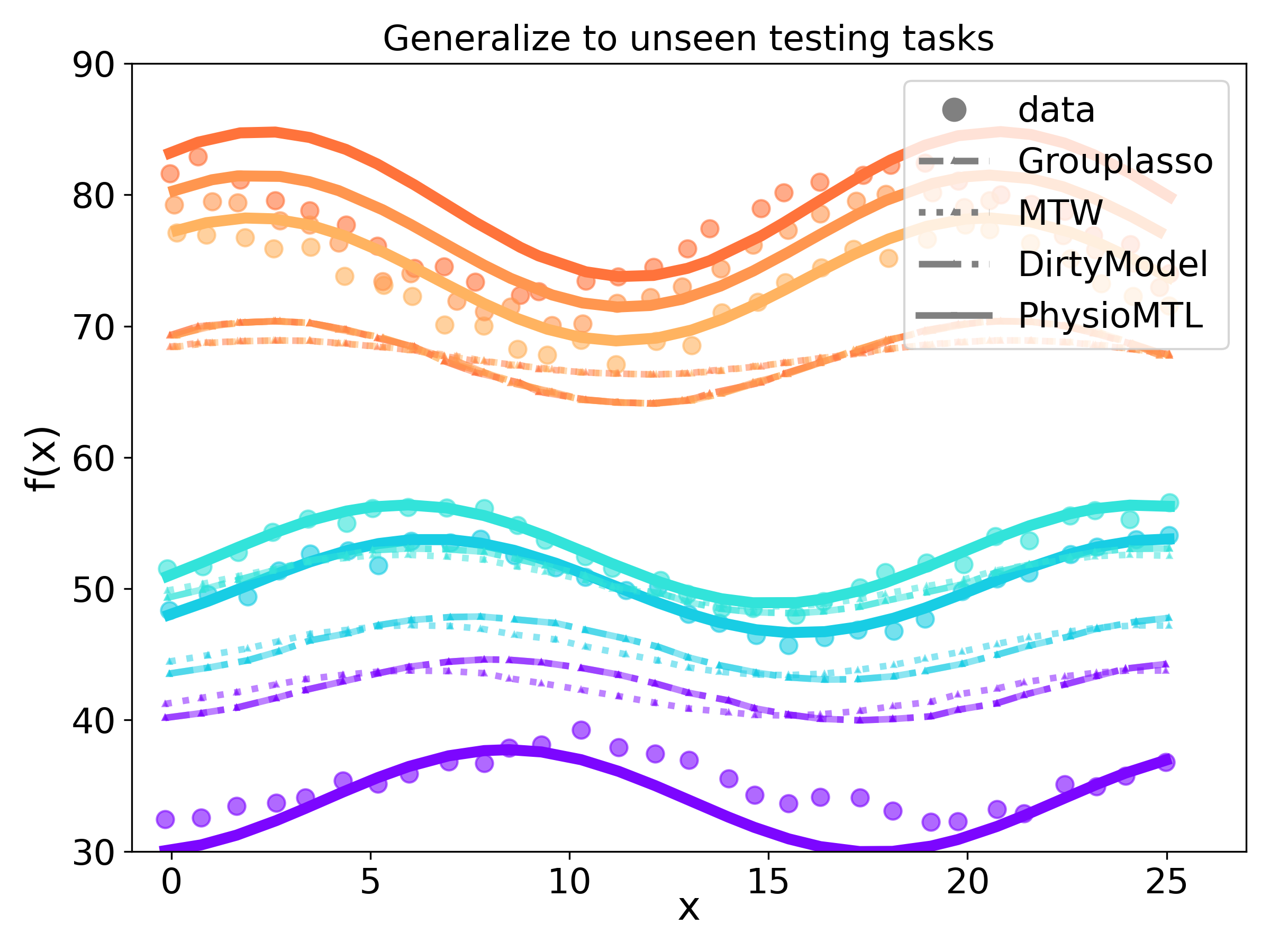
Figure 2: Qualitative illustration of PhysioMTL on simulated dataset (best viewed in color). Here each task is marked by color according its task-specified feature visualized in (b). In (a), We can see that the curves are varying smoothly with respect to this feature. In (b), we visualize the distribution of both training and testing tasks as $u(s_{t})$ and $v(s_{e})$ through kernel density estimation (KDE), and we can see the testing tasks have a small overlap with the training tasks. In (c), we show the prediction result of several baselines and our method. While other methods struggles to provide accurate prediction, our method (PhysioMTL) effectively generalizes to the out-of-sample unseen testing tasks.

3.4 Modeling HRV circadian rhythms

In practice, HRV data collected with mobile devices are unevenly distributed across time, thus challenging the application of most sequential machine learning models that assume evenly spaced data. Physiological studies  (Jarczok et al., 2019; Berger et al., 1986) have suggested to model the nonlinear circadian rhythm with a sinusoidal pattern (e.g., a cosinor model). For an individual $t$, the daily HRV circadian rhythm over a 24 hour period can be written as the following nonlinear function:

$$\begin{split}hrv(\tau)=M_{t}+A_{t}\sin(\frac{2\pi\tau}{P}+\phi_{t})+\epsilon_{t}(\tau)\vskip 3.0pt plus 1.0pt minus 1.0pt\end{split}$$ (9)

where $M_{t}$ is the Midline Statistic of Rhythm (MESOR), $A_{t}$ is the amplitude, $\phi_{t}$ is the phase shift and $\epsilon_{t}$ is the noise. Assuming the period $P$ is fixed, the model in Eq.(9) can be transformed into a linear model by expanding the sine term into $x_{1}=\sin(\frac{2\pi}{P}\tau)$, $x_{2}=\cos(\frac{2\pi}{P}\tau)$, yielding

$$\begin{split}hrv(\tau)=w_{0t}+w_{1t}x_{1}+w_{2t}x_{2}+\epsilon(\tau),\\ \end{split}$$ (10)

where $w_{0t}=M_{t}$, $w_{1t}=A_{t}\cos(\phi_{t})$, $w_{2t}=A_{t}\sin(\phi_{t})$. Given raw HRV measurements $\{h_{t,i},\tau_{i}\}_{i=1}^{n_{t}}$ of one subject $t$, we can learn parameters of the circadian rhythm model as a linear regression by rewriting $\mathbf{X}_{t}=[\mathbf{x}_{t,1}^{\top},...,\mathbf{x}_{t,n_{t}}^{\top}]\in\mathbb{R}^{n_{t}\times 3}$ where $\mathbf{x}_{t,i}=[\sin(\frac{2\pi}{P}\tau_{i}),\cos(\frac{2\pi}{P}\tau_{i}),1]$ and $\mathbf{Y}_{t}=[h_{t,i},..,h_{t,n_{t}}]^{\top}\in\mathbb{R}^{n_{t}\times 1}$. The benefit of this physiology-informed sinusoidal process is threefold: (1) The estimated sinusoidal parameters can serve as a personalized determination of circadian variation, (2) with a continuous function of time, we can assess underlying ANS status with unevenly sampled HRV measurements, and (3) the linear model naturally fits into a multi-task regression enabling estimation of the relatedness among a population of subjects.

Input: Data $\{X_{t},Y_{t},S_{t}\}$, cost function $C_{s}(s_{i},s_{j})$

Output: $\{\mathbf{W}=\{W_{1},W_{2},...,W_{t}\},\mathbf{F}\}$

for $t=1$ to $T$ do

       Solve $W_{t}$ by Linear Regression on $\{X_{t},Y_{t}\}$;

      

end for

Obtain the cost matrix $\tilde{\mathbf{C}}_{i,j}=C_{s}(s_{i},s_{j})$;

Solve the OT plan with equation (12);

while not converge do

       Update $F$ using gradient descent;

       Update $W$ using gradient descent;

end while

Algorithm 1 Joint Learning of $\mathbf{W}$ and $F$

3.5 Optimization algorithm and computation

The problem we address is to simultaneously learn the MTL parameters $\mathbf{W}$ and estimate $\pi$ and $\mathbf{F}$ for the associated OT formulation. The objective is given by combining equation (1) and equation (6):

$$\min_{\mathbf{W},\mathbf{F},\pi}\frac{1}{2}\sum_{t=1}^{T}\|W^{T}_{t}X_{t}-y_{t}\|^{2}_{2}$$

$$+\alpha\sum_{i,j=1}^{T}\pi_{i,j}c(F(\mathbf{s}_{i}),W_{j})$$ (11)

The formulation is jointly convex in each variable $\mathbf{W}$, $\mathbf{F}$, and $\pi$ when the remaining are fixed. Therefore, we solve the optimization problem with an alternating minimization framework.

3.5.1 Entropic OT & Prior on task similarity

When fixing $\mathbf{W}$, the second term of equation (3.5) is related to a category of OT formulation that can be solved by alternatively minimizing (Alvarez-Melis et al., 2019) over coupling $\pi$ and transformation $\mathbf{F}$. Specifically, when solving for $\pi$ with $\mathbf{W}$ and $\mathbf{F}$ fixed, the objective of equation (3.5) becomes an $O(n^{3}\log n)$ linear program. Here, adding an entropy regularization will allow us to use the celebrated Sinkhorn algorithm Ag.(2) (Cuturi, 2013) that just requires $O(n^{2})$ operations (Genevay et al., 2019), as:

$$\pi^{*}=\arg\min_{\pi\in\Pi}\sum_{i,j=1}^{T}\pi_{i,j}{\mathbf{C}}_{i,j}+\gamma H(\pi),$$ (12)

where $\mathbf{C}$ is a cost matrix, $H(\pi)=\sum_{i,j=1}^{T}\pi_{i,j}\log\pi_{i,j}$ is the negative entropy, and $\gamma$ is a coefficient such that $\gamma\xrightarrow{}0$ recovers the solution to equation (4). More details on the Sinkhorn algorithms are in the appendix.

We propose to further ease the computational burden by directly incorporating prior knowledge on the similarity of task-wise features. We pre-compute an optimal transport coupling $\pi^{*}$ with a cost matrix $\tilde{\mathbf{C}}_{i,j}=C_{s}(s_{i},s_{j})$ whose cost function $c_{s}:\mathcal{S}\times\mathcal{S}\mapsto\mathbb{R}^{+}$ is defined as

$$c_{s,ij}=\langle\mathbf{m},|\mathbf{s}_{i}-\mathbf{s}_{j}|\rangle,$$ (13)

where $\mathbf{m}\in\mathbb{R}^{d_{s}\times 1}$ is the similarity coefficient. Afterwards, the Sinkhorn algorithm approximates the optimal solution of equation (4), and we set $\pi=\pi^{*}$ during the learning procedure. This allows us to leverage prior domain knowledge when specifying task similarity (e.g., in our physiological example, we can weight chronic factors higher than acute stressors in our cost function). Note that $\mathbf{m}$ is also a potentially learnable parameter (Carlier et al., 2020; Stuart and Wolfram, 2020), however we leave the learning of $\mathbf{m}$ to future work.

3.5.2 Optimization and computation

With the task-similarity probabilistic coupling $\pi^{*}$ obtained, our final objective is given by:

$$\min_{\mathbf{W},\mathbf{F}}\frac{1}{2}\sum_{t=1}^{T}\|W^{T}_{t}X_{t}-y_{t}\|^{2}_{2}$$

$$+\alpha\sum_{i,j=1}^{T}\pi^{*}_{i,j}\|F(\mathbf{s}_{i})-W_{j}\|_{2}^{2}.$$ (14)

Here we use $l_{2}$ norm as the ground metric for model parameters. We thus solve the objective with Algorithm (1), which alternates between minimization of $\mathbf{W}$ and minimization of transport map $\mathbf{F}$. Notice that, when instantiating $\mathbf{F}$ to be in the class of linear mappings, minimization with respect to $\mathbf{F}$ has a closed-form solution as it corresponds to an Orthogonal Procrustes problem (Gower et al., 2004). However, here we are primarily interested in the case where $\mathbf{F}$ is a nonlinear kernel map. Therefore, for the chosen parameterization of $\mathbf{W}$, we use gradient descent to solve for the $\mathbf{F}$. While one could employ an arbitrary kernel, for simplicity we consider the commonly-used Radial Basis Function (RBF) kernel $k(x,x^{\prime})=\exp\left(-\frac{\|x-x^{\prime}\|^{2}}{2\sigma^{2}}\right)$ to conduct the kernel trick for a non-linear map. The effectiveness of the non-linear map depends on a proper length scale $\sigma$, and we recommend using cross-validation to select the optimal $\sigma$. For faster convergence in practice, we initialize $\mathbf{W}$ with prediction models learned independently from each task. More details on the computation, including the derivation of the gradients, can be found in appendix (B).

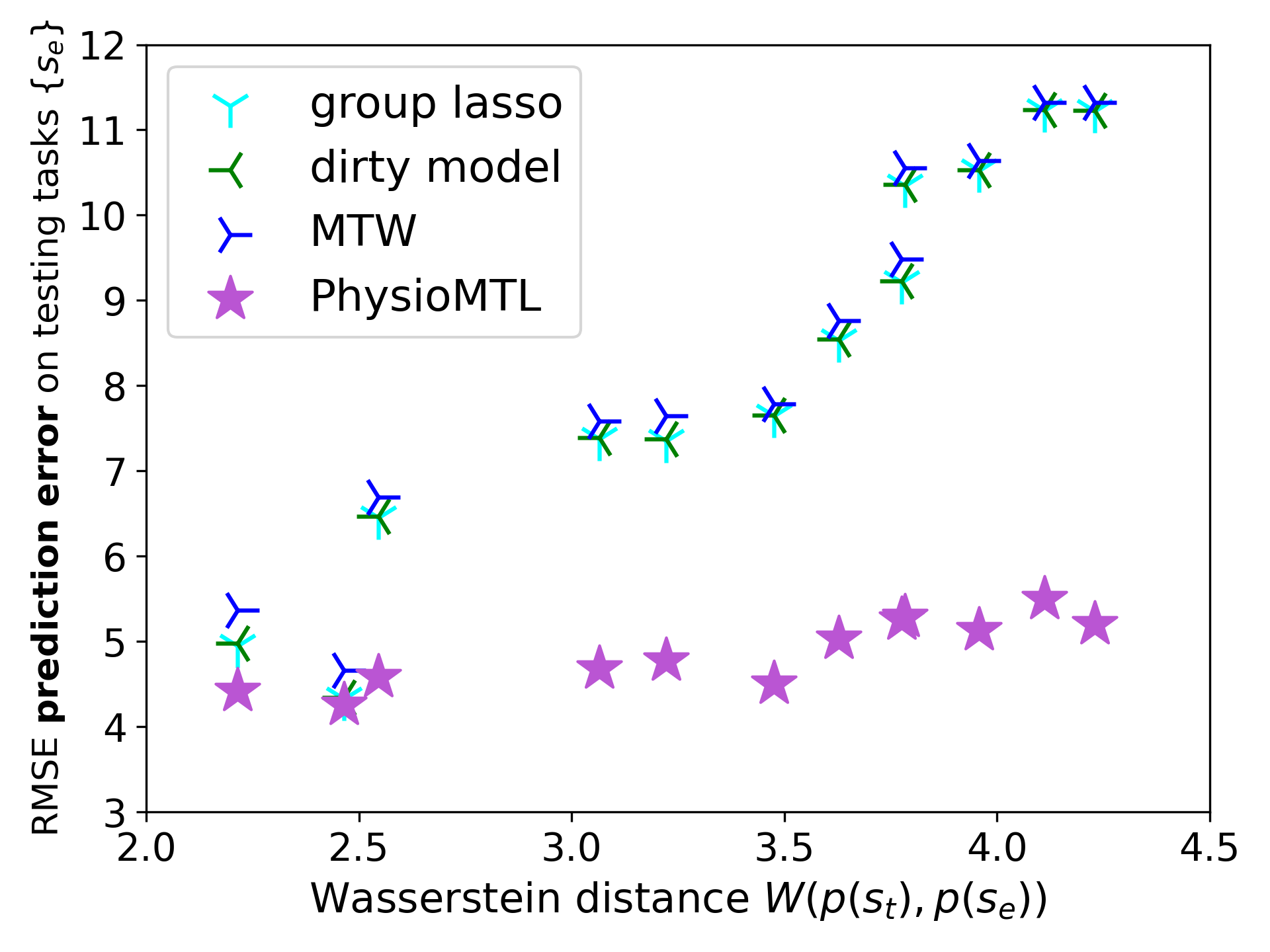
Figure 3: The prediction error (RMSE) versus the Wasserstein distance between the training and testing tasks $W(\mu(s_{t}),\nu(s_{e}))$ with Group Lasso, Dirty models, multi-task Wasserstein (MTW) and our proposed PhysioMTL.

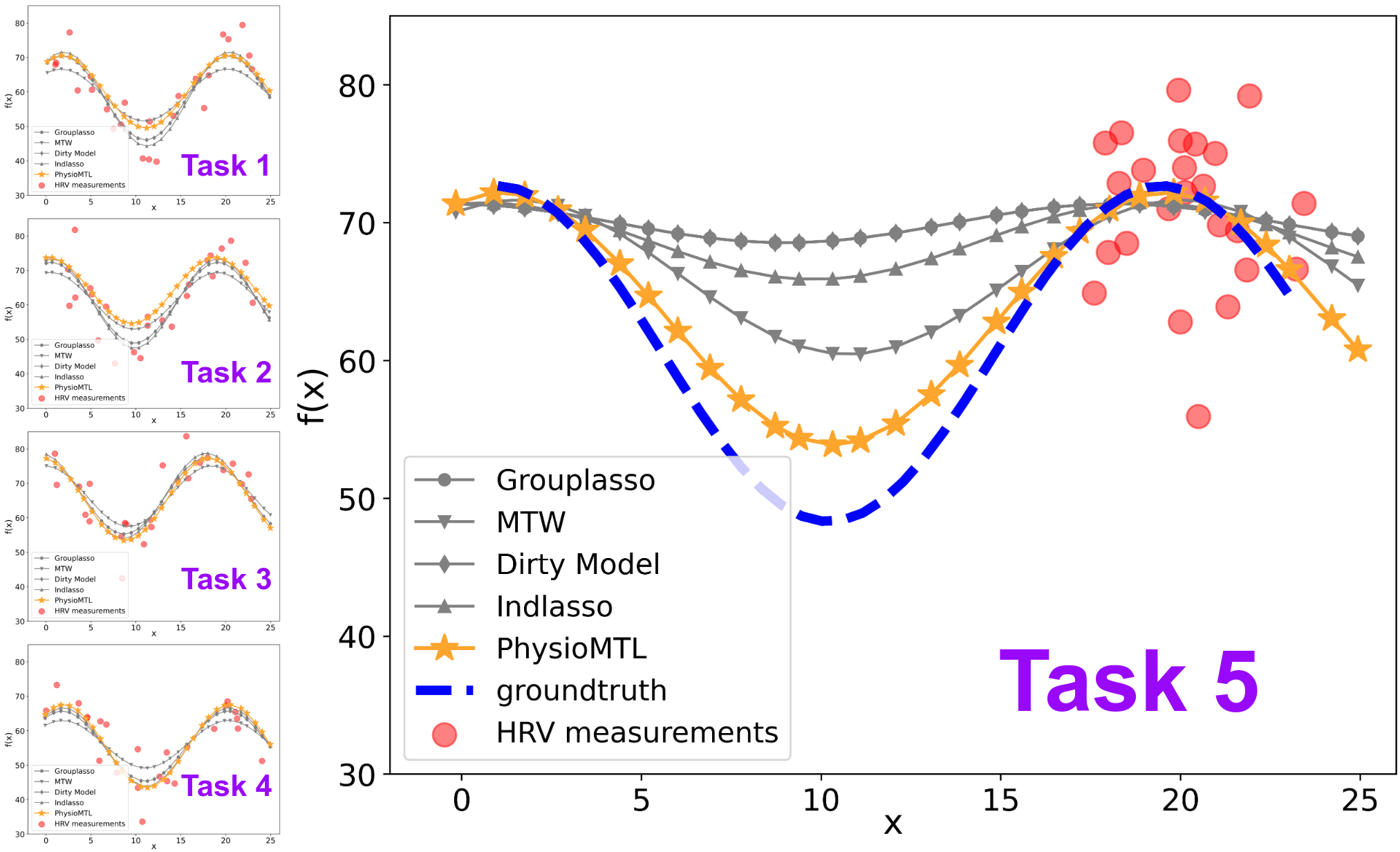
Figure 4: Example of generalization beyond an observed domain when measurements are limited to a particular time period. Tasks one through five are training data for each model; however, task five is missing data from a significant portion of the domain. PhysioMTL extrapolates most accurately to the true latent pattern.

4 Experiments

In this section, we first verify our proposed PhysioMTL on a synthetic dataset and then apply our method to two real-world datasets. In the first set of experiments, we illustrate how our proposed method adapts to unobserved tasks by comparing the distribution divergence between the training and testing tasks. We also quantitatively verify the advantages of our method over a set of baseline models. Second, we conduct a suite of experiments on two real-world physiology study datasets: the AHMS and MMASH datasets.

In addition to the quantitative evaluations that are standard for machine learning-based methodologies, we show that optimal transport captures meaningful underlying physiology mechanisms and discovers the effects of multiple cardiovascular risk factors from the data. There have been studies focusing on the effects of various cardiovascular risk factors, including age & gender (Abhishekh et al., 2013; Voss et al., 2015), BMI (Koenig et al., 2014), smoking (Murgia et al., 2019), and anxiety (Chalmers et al., 2014). However, most prior work focuses on one or two factors. Comprehensively analyzing multiple factors remains the goal of the current work. There is also a related and growing interest in applying counterfactual-based causal inference (Prosperi et al., 2020) methods to observational healthcare data. Towards this goal, a few pioneer works (Tu et al., 2021; Li et al., 2021) have explored the usage of OT in causal inference. In our study, we perform a conceptual counterfactual analysis by investigating the effect of each factor while holding the remaining fixed. To the best of our knowledge, this is the first study that simultaneously reveals the HRV rhythm variation caused by this set of cardiovascular factors (age, BMI, sleep, activity, VO2_max, and stress level).

Method	hyperparameter	$80\%$	$60\%$	$40\%$	$20\%$
Global Average	n/a	38.353 $\pm$ 4.925	35.998 $\pm$ 3.793	36.941 $\pm$ 1.877	36.918 $\pm$ 0.717
Single Lasso	$\alpha=0.9$	38.306 $\pm$ 5.972	35.693 $\pm$ 4.852	37.668 $\pm$ 3.110	36.187 $\pm$ 1.363
Multi-task Group lasso	$\alpha=0.9$	38.590 $\pm$ 5.978	35.948 $\pm$ 4.815	37.928 $\pm$ 3.093	36.457 $\pm$ 1.376
Multi-level lasso	$\alpha=0.9$	38.644 $\pm$ 5.999	35.996 $\pm$ 4.810	37.999 $\pm$ 3.099	36.509 $\pm$ 1.393
Dirty model	$\alpha=0.9$	38.582 $\pm$ 5.970	35.940 $\pm$ 4.818	37.921 $\pm$ 3.098	36.457 $\pm$ 1.377
MTW	$\alpha=0.9$	37.896 $\pm$ 5.743	35.354 $\pm$ 4.952	37.304 $\pm$ 3.084	36.170 $\pm$ 1.303
ReMTW	$\alpha=0.9$	37.941 $\pm$ 5.754	35.392 $\pm$ 4.941	37.349 $\pm$ 3.082	36.187 $\pm$ 1.307
PhysioMTL (linear)	$\alpha=0.1$	36.983 $\pm$ 5.181	35.167 $\pm$ 4.419	36.688 $\pm$ 2.521	36.525 $\pm$ 0.754
PhysioMTL (kernel)	$\alpha=0.1,l_{k}=20$	37.343 $\pm$ 5.173	34.379 $\pm$ 4.637	36.234 $\pm$ 2.298	35.677 $\pm$ 1.522

Table 1: Out-of-sample HRV prediction results on the AHMS dataset, evaluated using RMSE. We randomly choose from a given percentage {$80\%$, $60\%$, $40\%$, $20\%$} of subjects for training and then evaluate the model on the remaining held-out test subjects. Best performance for each percentage of training data is bolded.

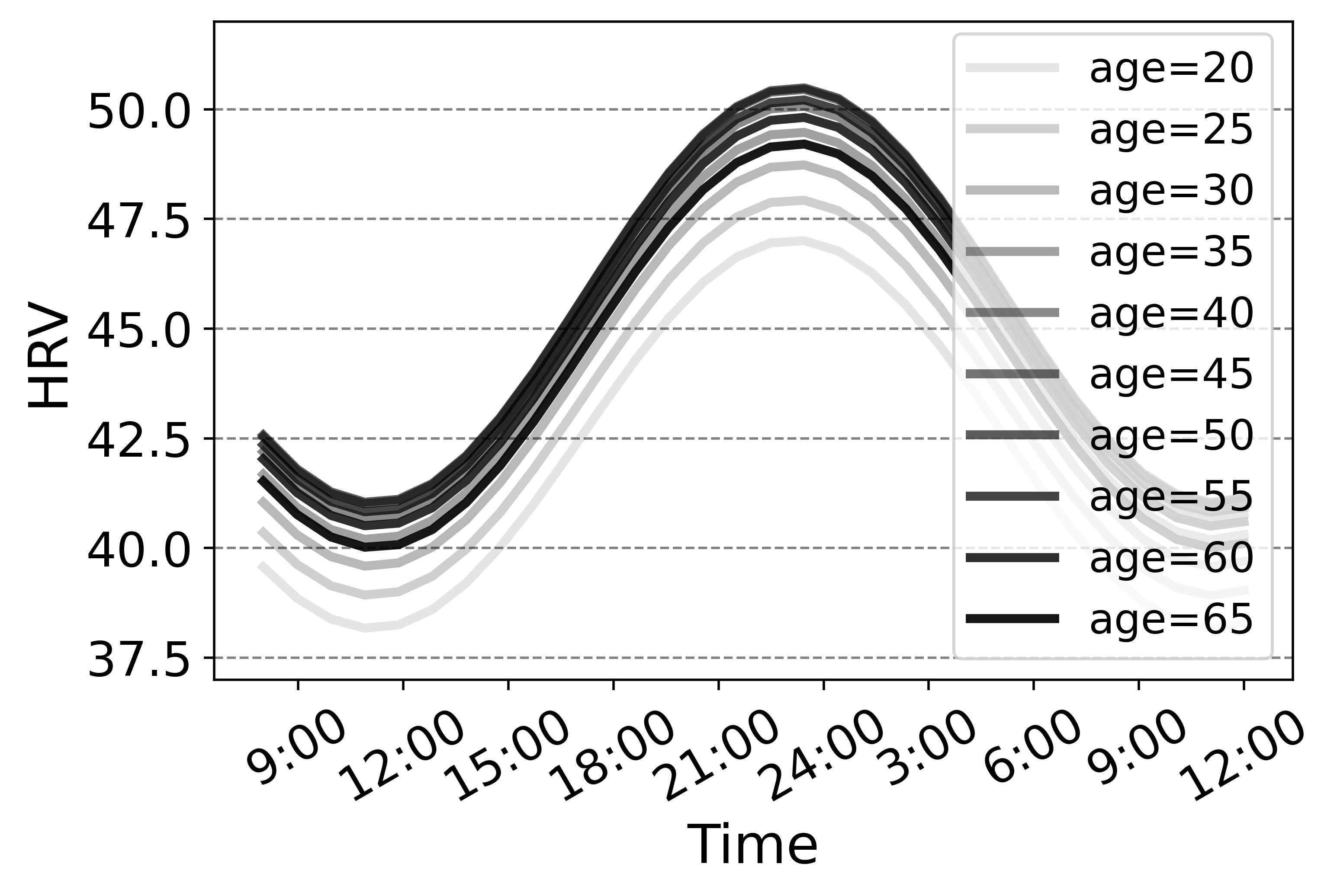
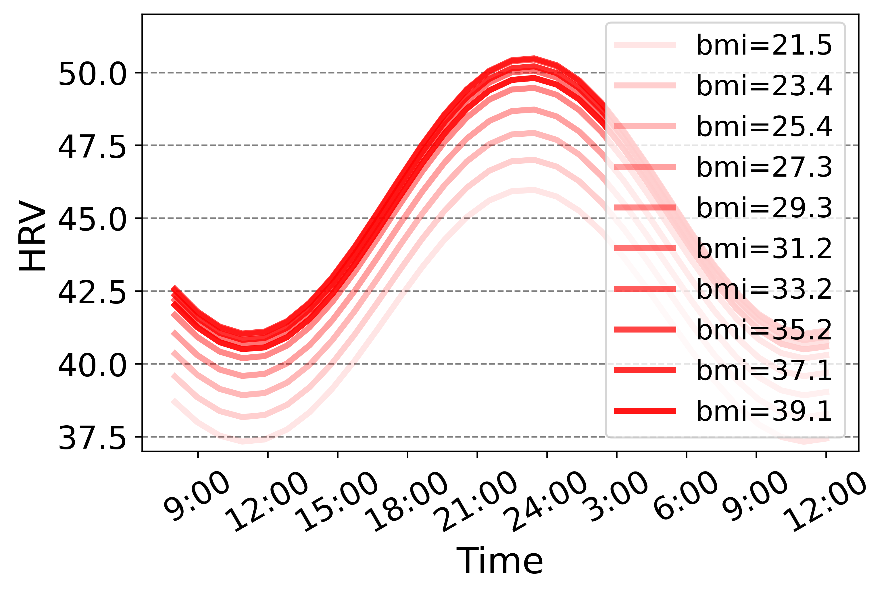
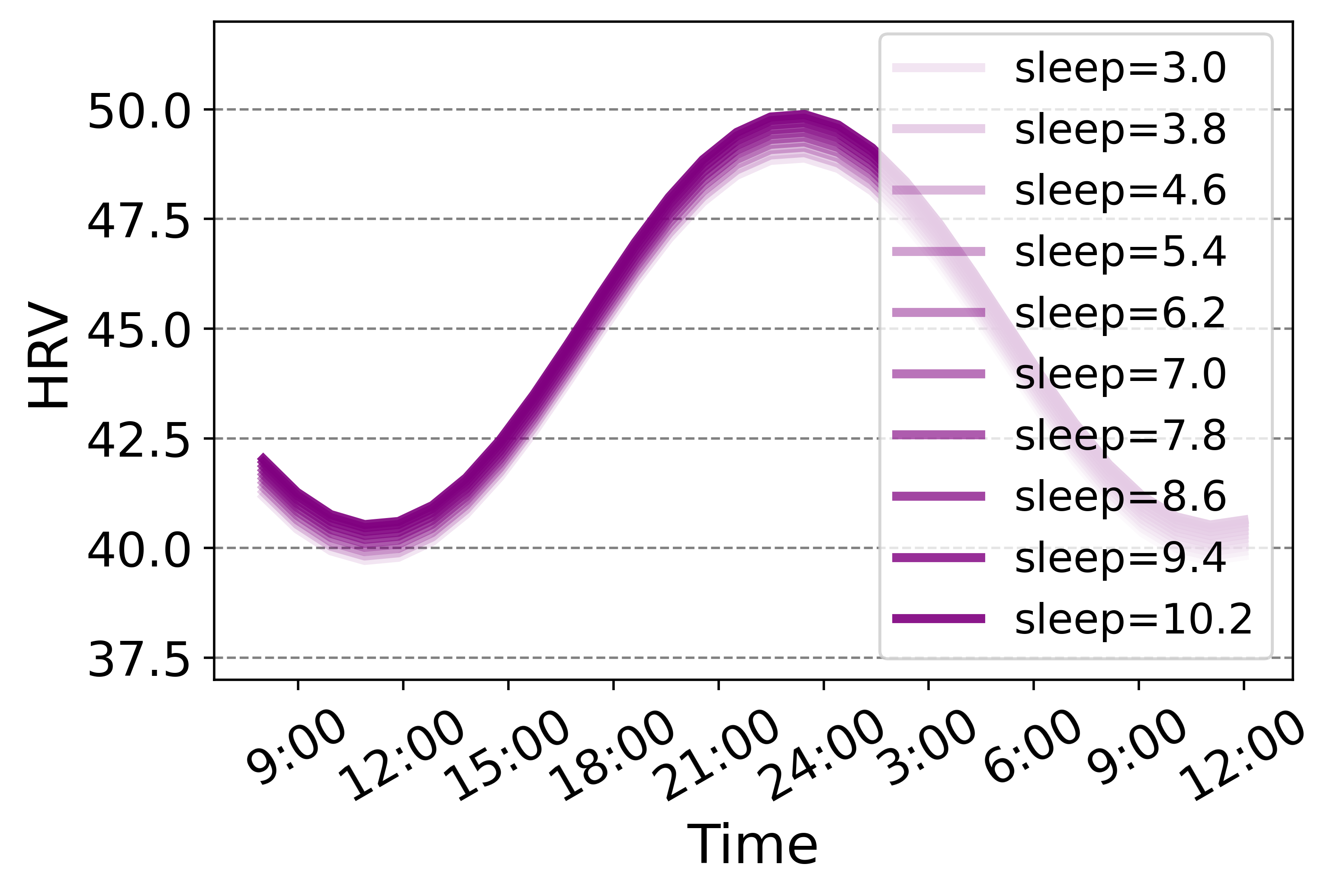
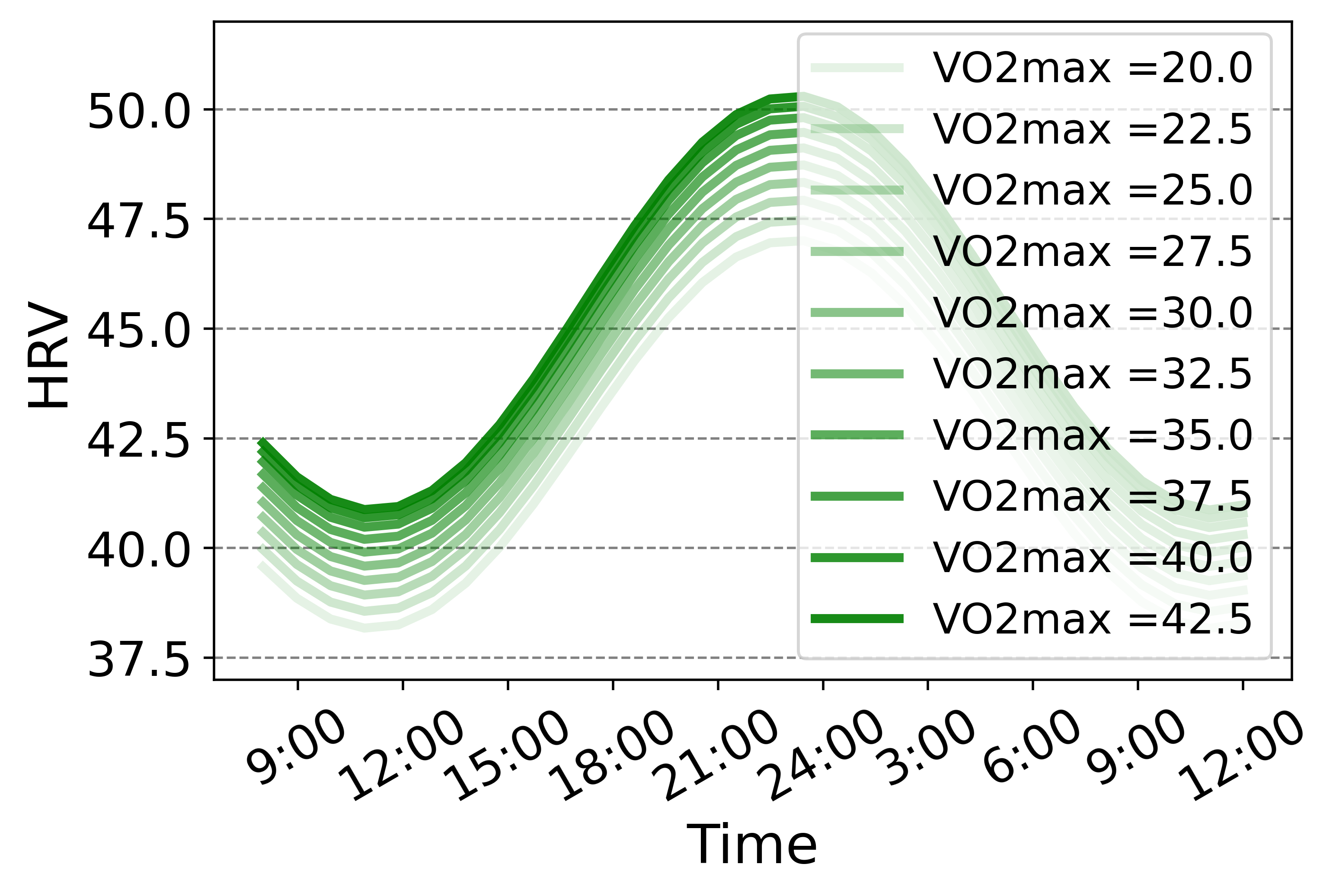
fig:ahms_kernel [Age] [BMI] [Activity]
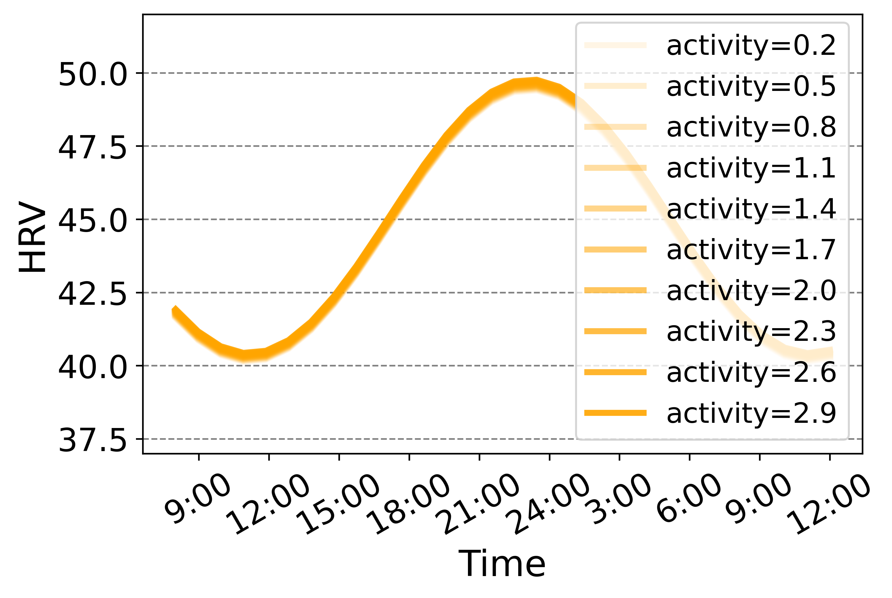
[Sleep] [VO2_max] [Baseline]

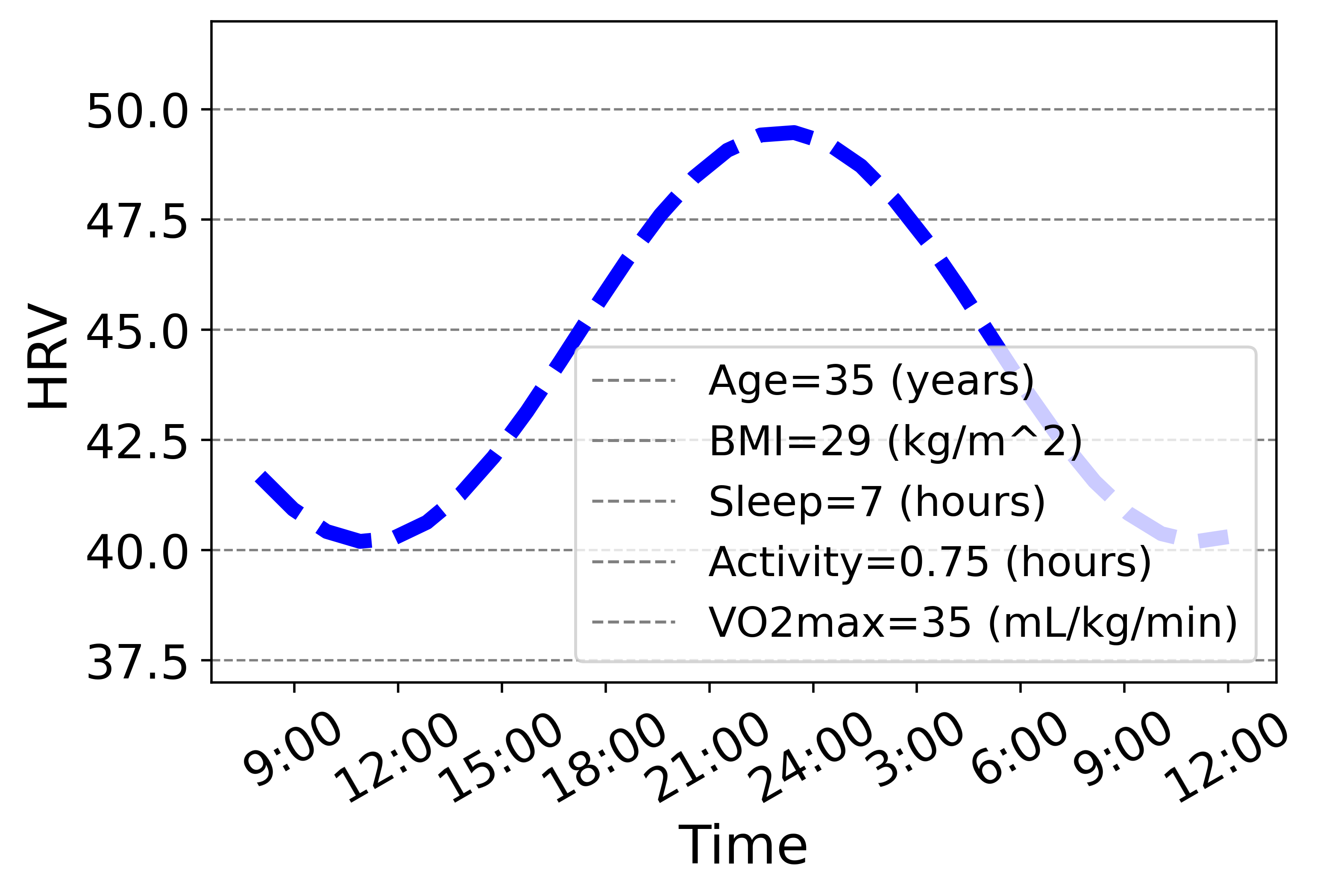
Figure 5: The counterfactual analysis on the AHMS dataset. We vary the attributes of a hypothetical subjective’s task-wise features and investigate the resulting HRV variational. Each feature investigated (age, BMI, activity, sleep, and VO2_max) is continuous, however, for ease of visualization we vary each feature on a discrete grid.

Method	hyperparameter	$80\%$	$60\%$	$40\%$	$20\%$
Global average	n/a	26.422 $\pm$ 3.490	26.622 $\pm$ 1.220	27.043 $\pm$ 1.613	26.998 $\pm$ 1.073
Single Lasso	$\alpha=0.9$	28.950 $\pm$ 3.740	28.498 $\pm$ 1.550	29.412 $\pm$ 1.657	28.812 $\pm$ 1.843
Multi-task Group Lasso	$\alpha=0.9$	28.816 $\pm$ 3.740	28.490 $\pm$ 1.529	29.177 $\pm$ 1.684	28.537 $\pm$ 1.817
Multi-level Lasso	$\alpha=0.9$	28.927 $\pm$ 3.728	28.627 $\pm$ 1.555	29.358 $\pm$ 1.664	28.758 $\pm$ 1.884
Dirty model	$\alpha=0.9$	28.816 $\pm$ 3.740	28.490 $\pm$ 1.528	29.176 $\pm$ 1.684	28.537 $\pm$ 1.816
MTW	$\alpha=0.9$	28.130 $\pm$ 3.802	27.689 $\pm$ 1.503	28.422 $\pm$ 1.832	27.953 $\pm$ 1.711
ReMTW	$\alpha=0.9$	28.175 $\pm$ 3.803	27.730 $\pm$ 1.508	28.464 $\pm$ 1.824	27.995 $\pm$ 1.716
PhysioMTL (linear)	$\alpha=0.1$	27.787 $\pm$ 3.066	28.358 $\pm$ 1.252	30.124 $\pm$ 1.644	33.453 $\pm$ 4.298
PhysioMTL (kernel)	$\alpha=0.1$, $l_{k}=20$	26.338 $\pm$ 3.371	26.470 $\pm$ 1.247	26.965 $\pm$ 1.660	26.875 $\pm$ 0.923

Table 2: Out-of-sample HRV prediction results on the MMASH dataset, evaluated using RMSE. We randomly choose from a given percentage {$80\%$, $60\%$, $40\%$, $20\%$} of subjects for training and then evaluate the model on the remaining held-out test subjects. Best performance for each percentage of training data is bolded.

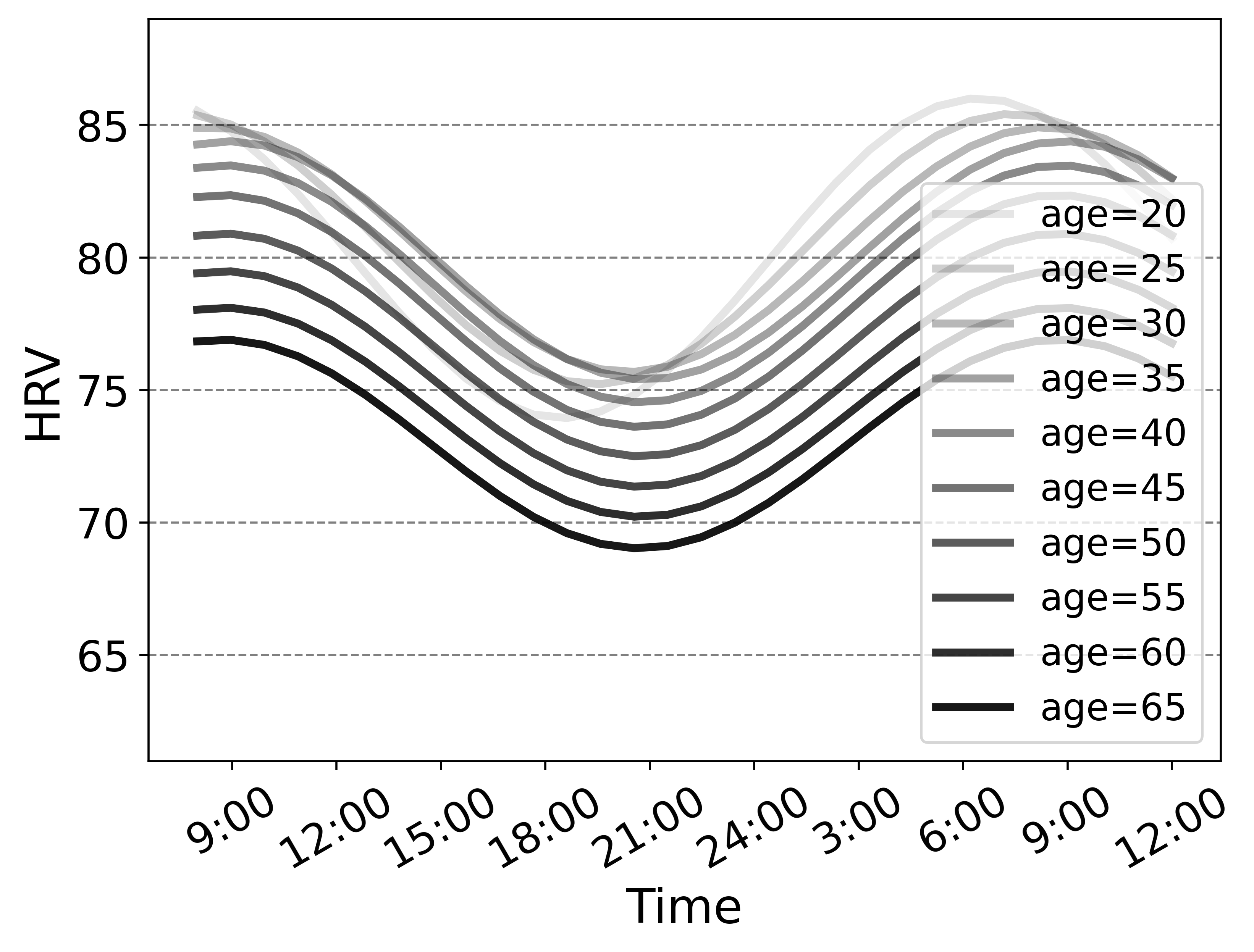
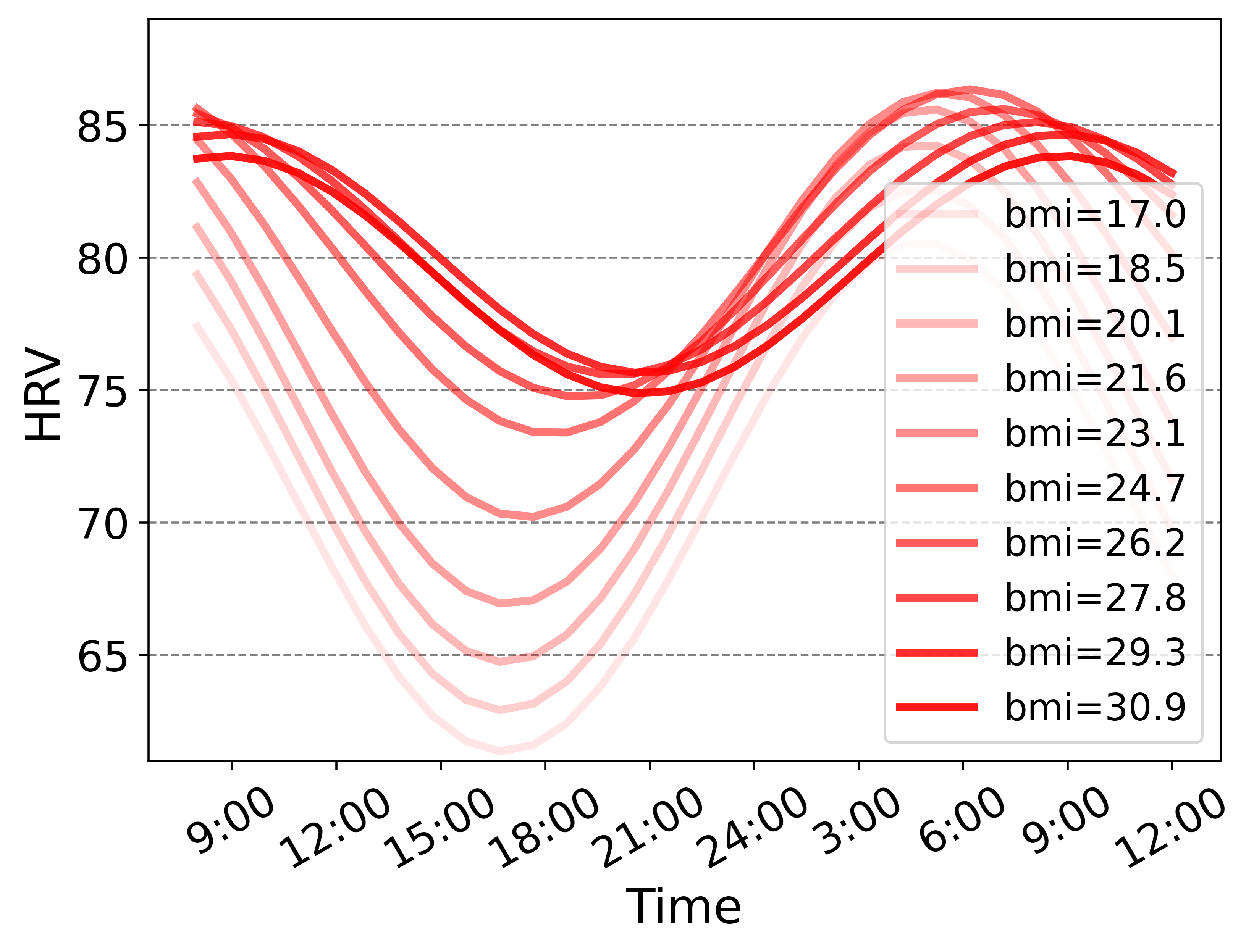
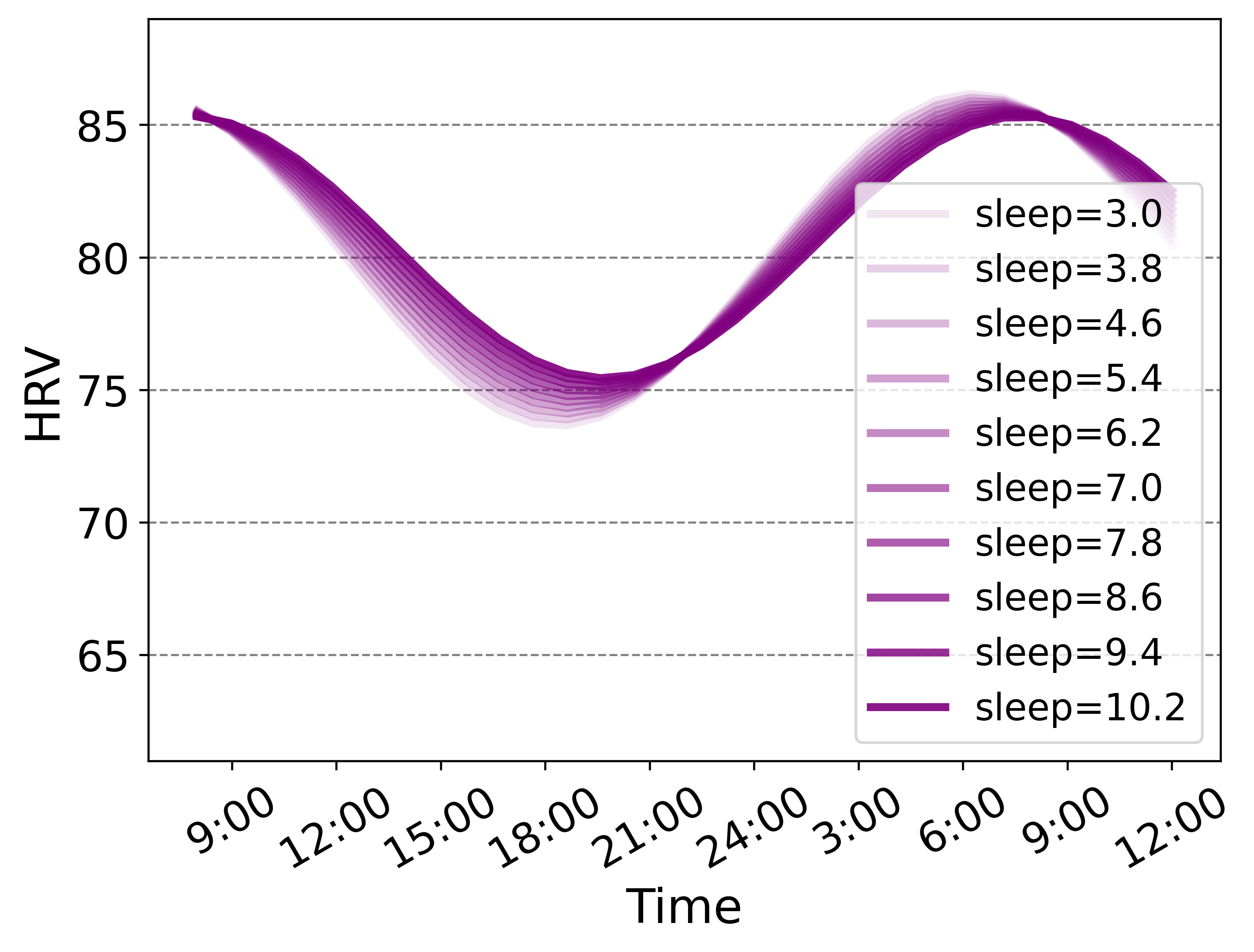
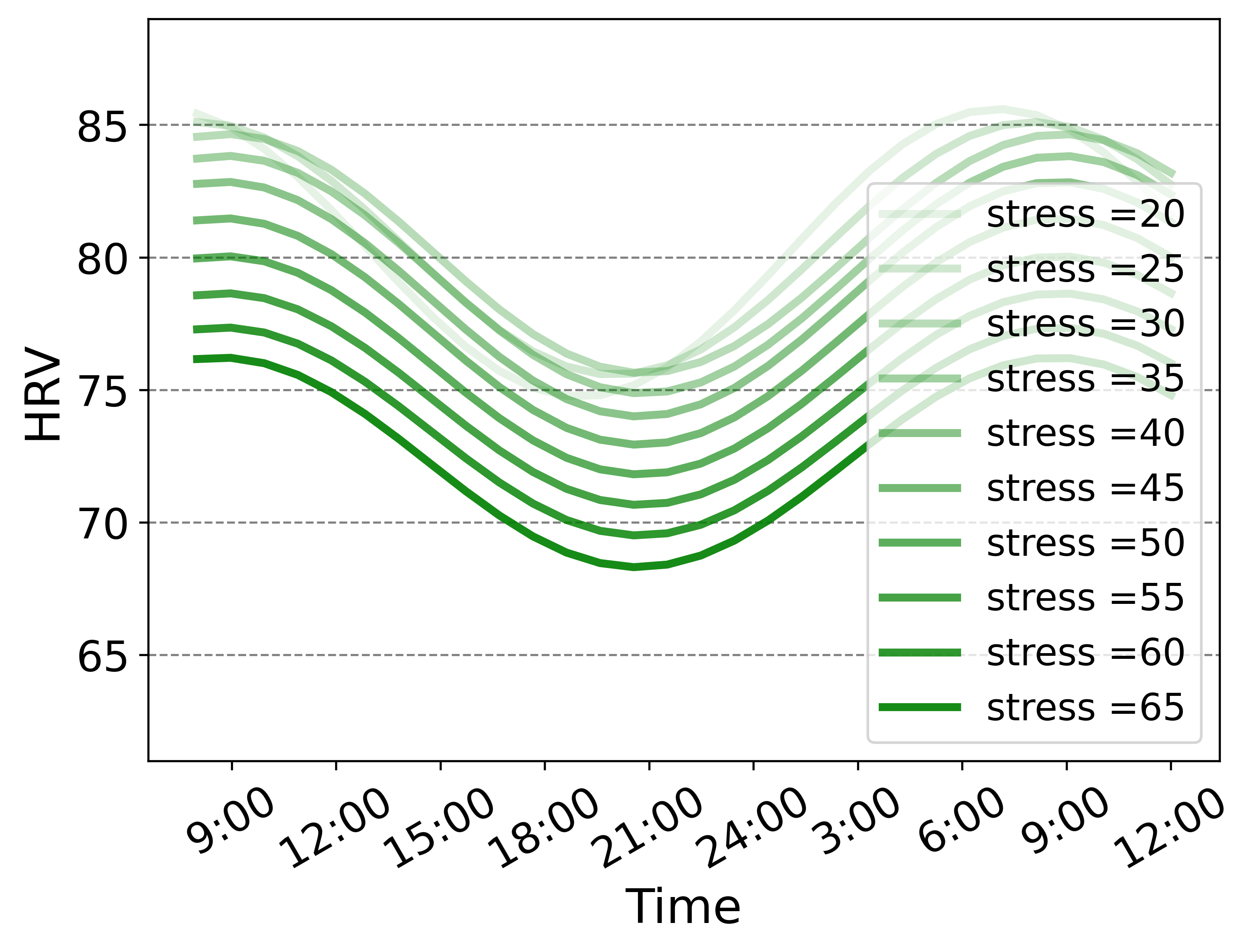
fig:mmash_kernel [Age] [BMI] [Activity]
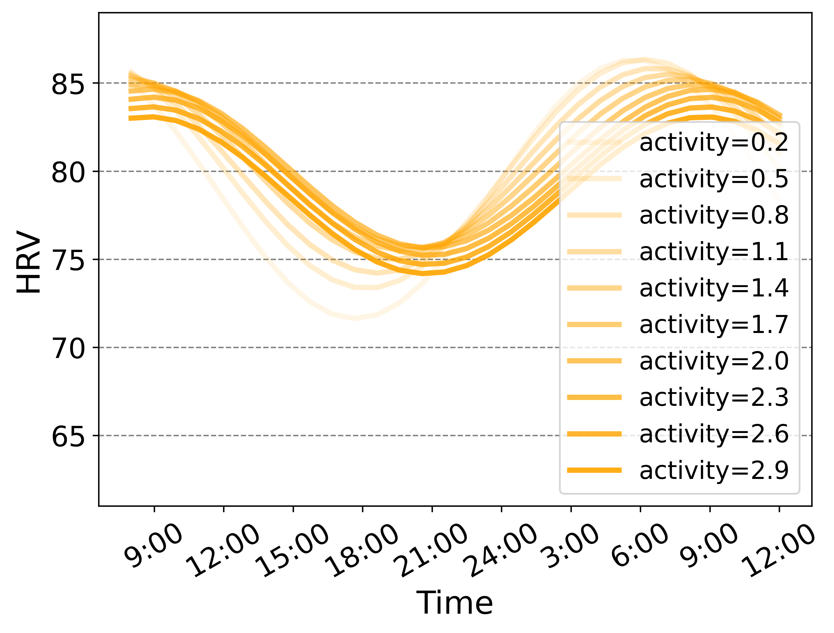
[Sleep] [Stress] [Baseline]

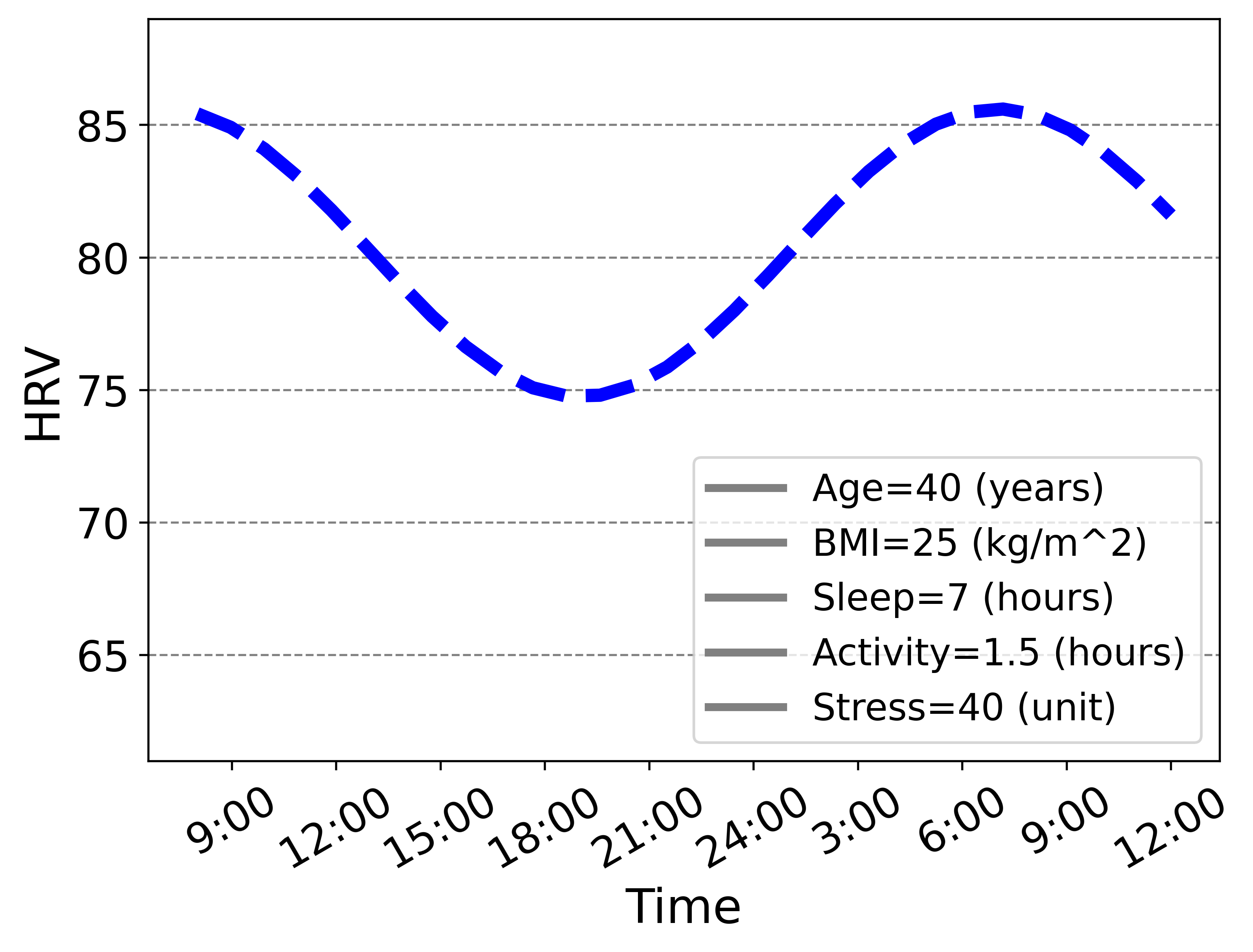
Figure 6: The counterfactual analysis on the MMASH dataset. We vary the attributes of a hypothetical subjective’s task-wise features and investigate the resulting HRV variational. Each feature investigated (age, BMI, activity, sleep, and stress) is continuous, however, for ease of visualization we vary each feature on a discrete grid.

4.1 Multi-task regression with synthetic data

We first sample the task-wise features via $s_{t,i}\sim U[p,q]$ where $p$, $q\in\mathbb{R}$ are hyperparameters that control the task distribution. Then we generate the feature-label pairs of each task via the following equation

$$y_{t,i}=m(s_{t})+A(s_{t})\sin(\frac{2\pi}{T}\tau_{t,i}+\phi(s_{t}))+e_{t,i}$$ (15)

where $m(s_{t})$, $A(s_{t})$ and $\phi(s_{t})$ are the groundtruth parameters for each task that are controlled by the task-wise feature $s_{t}$ by $m=a_{m}+b_{m}\times s_{t}$, $A=a_{A}+b_{A}\times s_{t}$ and $\phi=a_{\phi}+b_{\phi}\times s_{t}$. Here $e_{t,i}\sim N(0,\sigma_{t}^{2})$ is the task-specific noise. Then we randomly split the data into training and testing tasks, $\{s_{t,i}\}_{i}^{n_{t}}$ and $\{s_{e,i}\}_{i}^{n_{e}}$, where $n_{t}$ and $n_{e}$ are the number of training and testing tasks respectively. To measure the similarity between the training and testing tasks, we use a 2-Wasserstein distance of uniform empirical measures $W(\mu(s_{t}),\nu(s_{e}))$, where a larger Wasserstein distance indicates a larger divergence between the training and testing tasks.

We compare the performance of our method against Group Lasso (Yuan and Lin, 2006), Multi-level Lasso (Lozano and Swirszcz, 2012), Dirty models (Jalali et al., 2010), Multi-task Wasserstein and Reweighted Multi-task Wasserstein (Janati et al., 2019). The prediction error of our method is lowest amongst all methods we compared across a range of divergences between training and testing data (Figure 3). Additionally, the prediction error of other methods increases as the divergence between the training and testing task becomes larger, however, our model error increases at a far slower rate. This experiment validates that PhysioMTL is generalizable to out-of-sample tasks. In addition, in Figure 4 we demonstrate that PhysioMTL exploits the information shared among tasks and performs well on a given task that has samples constrained to a limited portion of time. Note that this is a quite common case in practice for wearable devices.

4.2 Experiments on real-world datasets

We conducted experiments on two real-world datasets: (1) the Apple Heart and Movement Study (AHMS) dataset and (2) the Multilevel Monitoring of Activity and Sleep in Health people (MMASH) dataset.

4.2.1 The AHMS dataset

The AHMS protocol allows participants to collect a comprehensive set of biometrics through wearable devices, thus providing a suitable dataset for studying the assessment of physiology status through wearable devices. In the AHMS dataset, HRV values are obtained by calculating the root mean square of successive differences between beat-to-beat measurements (RMSSD) captured by a heart rate sensor. Heart rate measurements are automatically recorded throughout the day while participants wear an activity tracker, thus there are multiple measurements each day. We obtain the task-wise feature vector for each subject as follows: the anthropometric characteristics including age, biological sex, height, and weight are self-reported by study participants. We use time in bed to indicate the sleep quality. We use hours of exercise to serve as an indicator of physical activity. We select a random set of subjects ($100$) that are split evenly between two self-reported genders (Female/Male), and have a minimum of 50 HRV measurements. We consolidate HRV measurements over a five month period of time because of the lack of measurement density within each 24 hour period, and average the demographic and lifestyle factors over that period if there are any changes.

4.2.2 The MMASH dataset

In the Multilevel Monitoring of Activity and Sleep in Healthy people (MMASH) dataset  (Rossi et al., 2020), $22$ healthy male subjects provided a set of 24 hours of continuous measurements including inter-beat intervals data, wrist accelerometry data, sleep time and quality data, physical activity data, psychological characteristics (e.g. anxiety status, stressful events, and emotion declaration).

Since HRV measurements are not directly provided, we first subdivide the inter-beat interval data into separate 5 minute intervals, and then we compute the RMSSD HRV (Shaffer and Ginsberg, 2017), which is the root mean square of successive differences between normal heartbeats, within each 5-minute interval. The length of interval is chosen as 5 minutes since it is the conventional short-time recording standard. We use the following attributes as task-wise features: Activity, Sleep, and Stress. Individual anthropometric characteristics such as Age, Height, and Weight are provided as well. We use total minutes in bed to denote the sleeping information and convert it to total hours in bed for consistency. The MMASH dataset provides an activity diary for each subject, we use the total hours of medium (e.g. fast walking and cycling) and heavy (e.g. gym, running) to indicate physical activity. Finally, each subject provides a subjective measure of stress denoted as the Daily Stress Inventory (DSI) score. We process the data with the following steps: (1) For each subject, we remove the outliers with z-score greater than $2.5$ after computing RMSSD HRV values from 5-minute intervals, (2) we exclude the subjects that have particularly abnormal measurements (i.e., subject 4 has an average RMSSD of $318$), and (3) since subjects 11 and 18 do not provide sleep data and age, respectively, these missing values are imputed with data-wide means. Our pre-processing led us to consider 21 out of 22 subjects.

4.3 Experimental procedure

To investigate the generalization, we evaluate the model on those tasks that are unobserved during training. We randomly split the tasks into training and testing task sets, and then evaluate the performance of each method using root mean square error (RMSE) of prediction. We repeat the selection-evaluation process for $n=10$ times and report the mean and standard deviation of each method’s RMSE. We select the $k$-nearest tasks for baseline MTL methods when predicting out-of-sample tasks. To enable a meaningful comparison, we use the same task similarity metric $C_{s}(\cdot,\cdot)$ for all MTL methods where we encourage all the attributes in the task-wise feature vector to have an equal influence on task similarity.

For experiments on the AHMS dataset, we use a global mean estimator and Lasso estimator independently run on each task as a baseline. We additionally compare Multi-task Lasso (Obozinski et al., 2006) and Multi-task Elastic-Net (Zou and Hastie, 2005) with our approach. For the MMASH dataset, we compare our method with Group Lasso (Yuan and Lin, 2006), Multi-level Lasso (Lozano and Swirszcz, 2012), Dirty models (Jalali et al., 2010), Multi-task Wasserstein and Reweighted Multi-task Wasserstein (Janati et al., 2019). We select the best hyperparameter $\alpha$ for all baseline methods.

4.4 Results and physiological patterns

4.4.1 Predictive performance

Our method has superior performance on both datasets compared with all baseline methodologies. The quantitative results on the AHMS dataset are given in Table (1). In Table (2), we provide a comprehensive comparison on the MMASH dataset. We test the extreme case where only ($20\%$) of tasks are available for training and found PhysioMTL with a nonlinear optimal transport map achieves the best performance. While PhysioMTL with a linear map is competitive across many scenarios, with a nonlinear transport map PhysioMTL has lower error than all other methods. It is worth mentioning that HRV measurements are extremely noisy and there exist numerous confounding variables. Therefore, even a small improvement of RMSE means a more accurate estimation of HRV circadian rhythm parameters. A more illustrative example is given in Figure (4), where the RMSE errors of all methods are similar, but the circadian rhythm estimated by the PhysioMTL is closer to the groundtruth.

4.4.2 Counterfactual analysis

The physiological constraints we encode in PhysioMTL allow us to investigate the affect of acute and chronic stressors on cardiovascular activity assessed through HRV. We can construct counterfactuals by setting a baseline task feature vector and varying one dimension at a time while holding the remaining dimensions constant.

In Figure (LABEL:fig:mmash_kernel), we display a set of HRV variations across several dimensions. In general, all the results are consistent with existing physiological studies. Age is a dominant factor, as aging in healthy subjects is typically associated with a decline in HRV. Our results also show aging will lead to a decrease in the circadian rhythm amplitude. We found BMI has a non-monotonic relationship to HRV mean value. Also, an increasing sleep hours will lead to a higher and more stable circadian rhythm. Interestingly, we observed the HRV pattern first goes up as activity increases and then decreases. This trend reflects the phenomenon that light endurance training increases acute HRV but higher exertion bouts can cause decreases in HRV (Plews et al., 2014). Finally, our model shows stress and anxiety present as lower values of HRV.

5 Conclusion

We investigate how acute and chronic factors affect HRV rhythms. We leverage established sinusoidal analysis of the ANS system and optimal transport theory to develop the PhysioMTL model. The tasks are viewed from a geometric and probabilistic perspective, and an optimal transport map captures a general correspondence between tasks that are similar and generalizes to unseen samples. We validate our method on synthetic and real-world physiological datasets and show our approach outperforms existing MTL methods. Our model learns an approximation of the true latent HRV pattern for each individual and serves as an accurate prediction for new individuals based on a few pieces of easily captured information.

Beyond prediction, our method lends itself to analyzing counterfactual scenarios. This allows us to investigate the hypothetical question of what underlying physiology would have presented as given an unobserved setting of features. We use this counterfactual to show the effect of our captured demographic and lifestyle covariates on HRV rhythms.

We note that we do not directly compare to meta-learning and transfer learning methods since we evaluate all methods on completely unseen tasks and do not consider a fine-tuning step on prediction tasks. However, the predicted function (model parameters) can actually serve as a prior initialization for an unseen task and enable fine-tuning on the target domain. Thus, our method can be considered a potentially general meta-learning formulation where the optimal transport map is a meta-learner. Towards this goal, future work will also consider extending our framework to more flexible and expressive models, such as function spaces modeled by deep neural networks. In this case, it may be possible to directly predict the parameters or learn suitable priors over the parameters of a task-specific neural network. We also consider the possibility of learning a larger network with a shared subcomponent that performs representation learning over tasks, and a task-specific subcomponent with priors learned from training data.

Finally, we study a single physiological indicator, HRV, since the diurnal patterns that serve as the baseline for our method are well-studied. The covariates we study have also been analyzed to some degree previously, thus there is prior evidence to support our findings. However, our framework is quite general. By changing the form of the individual task regressor and the task relatedness kernel, our methodology could be used to investigate a number of other physiological and non-physiological signals where captured covariates are thought to explain a fair amount of variation in the signal. A further extension to our work could jointly model multiple signals in order to share predictive power captured in the covariates across multiple associated signals.

Institutional Review Board (IRB)

The Apple Heart and Movement study was conducted in collaboration between Apple and Brigham and Women’s hospital, the data were collected in accordance with an Advarra IRB approved study protocol.

We would like to thank Guillermo Sapiro, Calum MacRae, Nick Foti, Russ Webb, Haraldur Hallgrímsson, Gary Shin, Laixi Shi, and Jielin Qiu for valuable feedback and comments on our manuscript.

Appendix A Further Literature Review

A.1 Machine learning for healthcare

The Spatio-temporal group lasso (STGL-MTL) (Romeo et al., 2020) encodes the task relatedness with a regularization term and a graph structure for diabetes prediction. Within the MTL framework, the combination of task labels can provide auxiliary tasks (Hsieh and Tseng, 2021) and aid in ECG phenotyping prediction. A temporal asymmetric MTL model (Nguyen et al., 2020) is proposed to enforce knowledge transfer only between relevant tasks to approach safety-critical scenarios such as clinical risk prediction. A multi-task generative model (Wang et al., 2020) has also been used for clinical topic modeling. Multi-view deep learning models are develop to deal with the multimodality of human emotion, electroencephalography (EEG) and electrocardiogram (ECG) (Qiu et al., 2018; Liu et al., 2021). Recently, Optimal Transport (OT) related methods (Qiu et al., 2022) have improved the performance of deep learning methods for electrocardiogram (ECG).

A.2 Multi-task learning and task relatedness

Various multi-task learning approaches have been developed to exploit the correlation among tasks. For instance, task clustering approaches (He et al., 2019; Zhou et al., 2011a) assume different tasks can be clustered. Feature sharing (Evgeniou and Pontil, 2007) and low-rank (Zhou et al., 2011b) approaches assume all tasks are related. Kernel-based methods (Bonilla et al., 2007) encode task-specific features to obtain task similarity and therefore enhance the prediction performance.

A.3 Intuition

To tackle domain adaptation limitations, we incorporate optimal transport map estimation theory with multi-task learning. Optimal transport (OT) (Villani, 2009) has attracted considerable interest in the machine learning community. OT provides a meaningful distance between probability measures that do not share the same support; OT also formulates a transport map (Zhu et al., 2021; Perrot et al., 2016; Alvarez-Melis et al., 2019) that pushes forward one distribution onto another. Also, the addition of entropic regularization (Cuturi, 2013) yields fast computation, thus enabling scalability of OT to larger problems.

Pop et al. (2021); Jarczok et al. (2019) have shown that those individuals that have similar demographic attributes exhibit a similar HRV pattern. To this end, we regard the observed individuals as empirical distributions evaluated from an underlying distribution and further assume a smooth transport map from the distribution of tasks to the distribution of predictive functions.

A.4 OT

the Monge problem consists in finding a Borel map, $T:\mathcal{X}\mapsto\mathcal{Y}$ between $\mu$ and $\nu$. that realizes the infimum

$$\inf_{T}\int_{\Omega}c(x,T(x))d\mu(x)\text{ \vskip 3.0pt plus 1.0pt minus 1.0pt{}{} subject to {}{} \vskip 3.0pt plus 1.0pt minus 1.0pt}T_{\#}\mu=\nu,$$ (16)

where $T_{\#}\mu$ denotes the push forward operator of $\mu$ by $T$. However, the existence of the optimal Monge map $T$ is not always guaranteed—the Monge problem is non-convex and often unfeasible, for example, when the support $\mu$ and $\nu$ are a different number of Dirac delta functions.

Appendix B Computational details

B.1 Derivation of computation algorithms

We give a local minima solution for the objective Equation. (3.5.2) by alternatively minimizing over W and F with regard the loss function:

$$L(\mathbf{F},\mathbf{W})=\frac{1}{2}\sum_{t=1}^{T}\|W^{T}_{t}X_{t}-y_{t}\|^{2}_{2}+\alpha\sum_{i,j=1}^{T}{\pi^{*}}_{i,j}\|\mathbf{F}\mathbf{s}_{i}-W_{j}\|_{2}^{2}.$$

The algorithm is described in Alg. (1) and we give the explicit calculations below. We will use the linear map in derivation but notice that for both ways of transport map parameterization (linear and kernel), the only difference is the size of the $\mathbf{F}$ matrix.

Updating $\mathbf{F}$ with $\mathbf{W}$ fixed: Here the minimization objective becomes

$$\hat{\mathbf{F}}=\arg\min_{\mathbf{F}\in\mathrm{R}^{d_{\theta}\times d_{s}}}L(\mathbf{F},\mathbf{W})=\arg\min_{\mathbf{F}\in\mathrm{R}^{d_{\theta}\times d_{s}}}\alpha\sum_{i,j=1}^{T}{\pi^{*}}_{i,j}\|\mathbf{F}\mathbf{s}_{i}-W_{j}\|_{2}^{2}.$$ (17)

We preform gradient descent method to achieve the minimum, where the gradient is:

$$\nabla_{\mathbf{F}}L(\mathbf{F},\mathbf{W})=2\alpha\sum_{i=1}^{T}\sum_{j=1}^{T}\pi^{*}_{i,j}(\mathbf{F}s_{i}-W_{j})s_{i}^{\top}.$$ (18)

Updating W with F fixed: Now we want to solve

$$\hat{\mathbf{W}}=\arg\min_{\mathbf{W}\in\mathrm{R}^{T\times d_{w}}}L(\mathbf{F},\mathbf{W})=\arg\min_{\mathbf{W}\in\mathrm{R}^{T\times d_{w}}}\frac{1}{2}\sum_{t=1}^{T}\|W^{T}_{t}X_{t}-y_{t}\|^{2}_{2}+\alpha\sum_{i,j=1}^{T}{\pi^{*}}_{i,j}\|\mathbf{F}\mathbf{s}_{i}-W_{j}\|_{2}^{2}.$$

Also, we use block gradient descent to obtain the solution, where the gradient is:

$$\nabla_{\mathbf{W}_{t}}L(\mathbf{F},\mathbf{W})=-(W_{t}X_{t}-y_{t})x_{t}^{\top}-\sum_{i=1}^{T}\pi^{*}_{i,t}(\mathbf{F}s_{i}-W_{t})$$ (19)

B.2 Entropic optimal transport and Sinkhorn algorithm

Input: Cost matrix $\mathbf{C}\in\mathbb{R}^{n\times m}$, entropy coefficient $\gamma$

Output: $\mathbf{\Pi}$

$\mathbf{K}\xleftarrow{}\exp(-\mathbf{C}/\gamma)$, $\mathbf{\nu}\xleftarrow{}\frac{\mathbf{1}_{m}}{m}$;

while not converge do

       $\mathbf{\mu}\xleftarrow{}\frac{\mathbf{1}_{n}}{n}\oslash\mathbf{K}\mathbf{\nu}$;

       $\mathbf{\nu}\xleftarrow{}\frac{\mathbf{1}_{m}}{m}\oslash\mathbf{K}^{T}\mathbf{\mu}$;

end while

$\mathbf{\Pi}\xleftarrow{}diag(\mathbf{\mu})\mathbf{K}diag(\mathbf{\nu})$;

Algorithm 2 Sinkhorn algorithm

Appendix C Additional experiments and details

C.1 Uneven time

As illustrated in figure (LABEL:fig:uneven_app), we overlay the regression results on a training set of 5 tasks where Task 5 is missing data from a significant portion of the domain. While all multi-task regression methods, including independent models, perform fairly well on tasks 1-4, only our proposed PhysioMTL method yields the most accurate regression result.

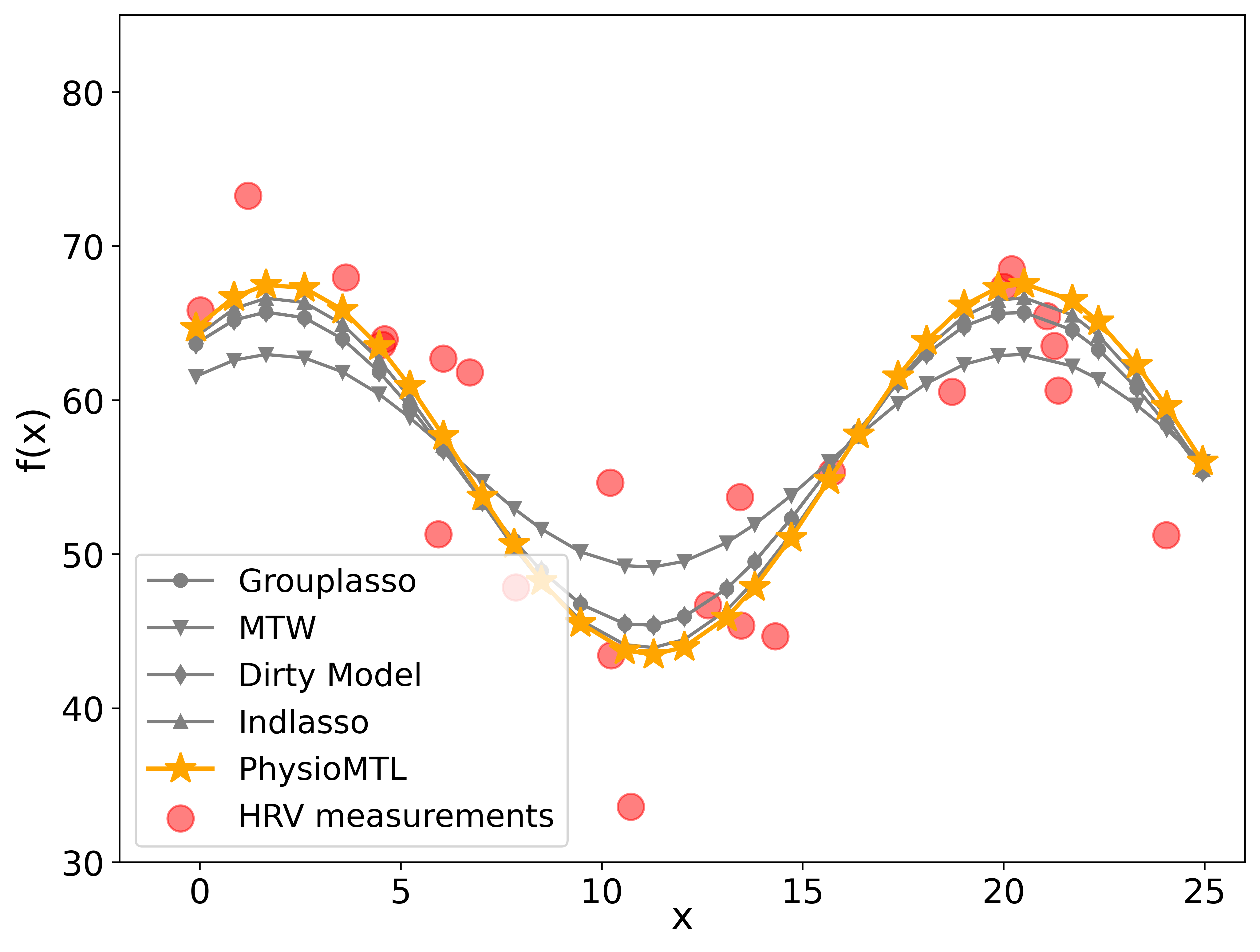
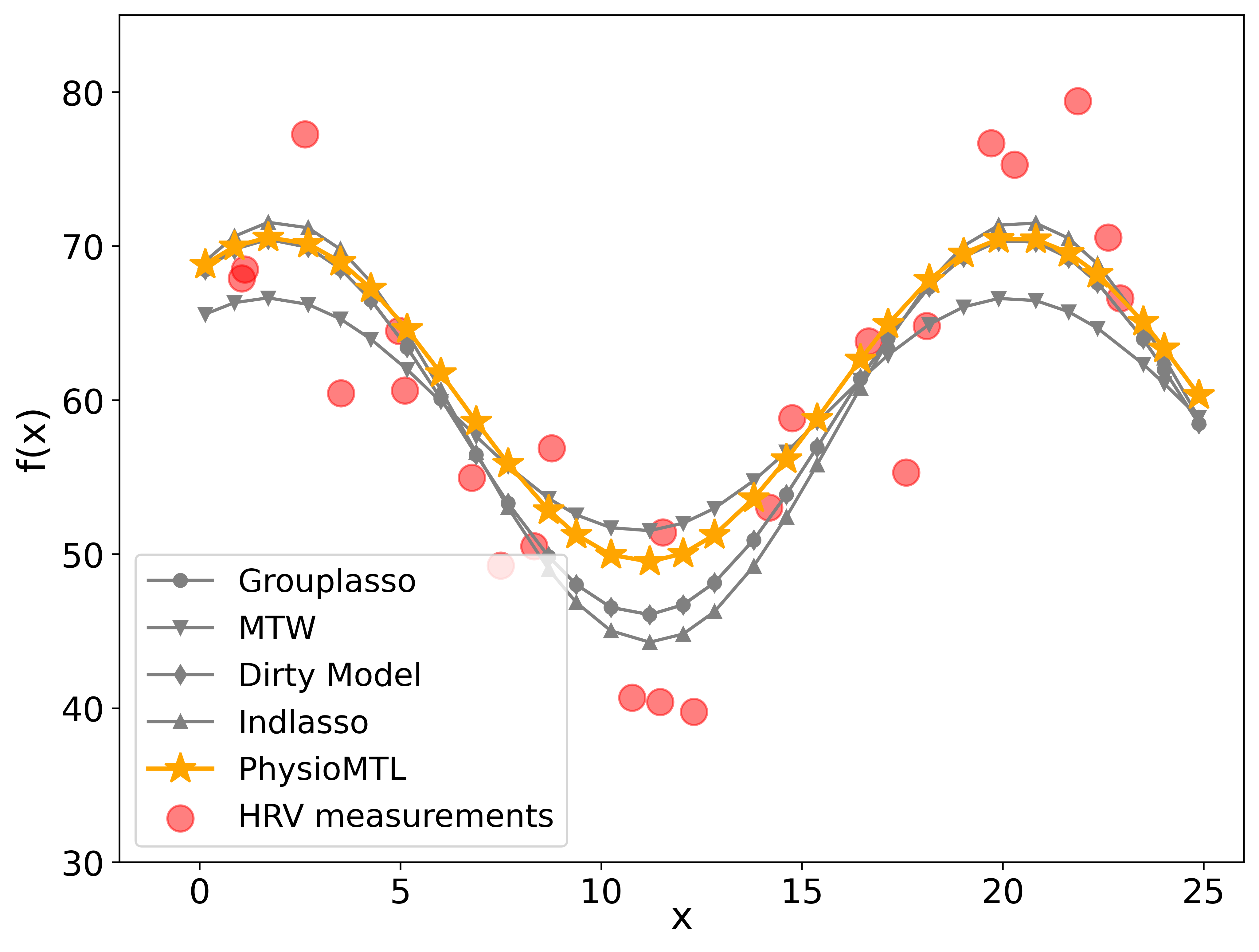
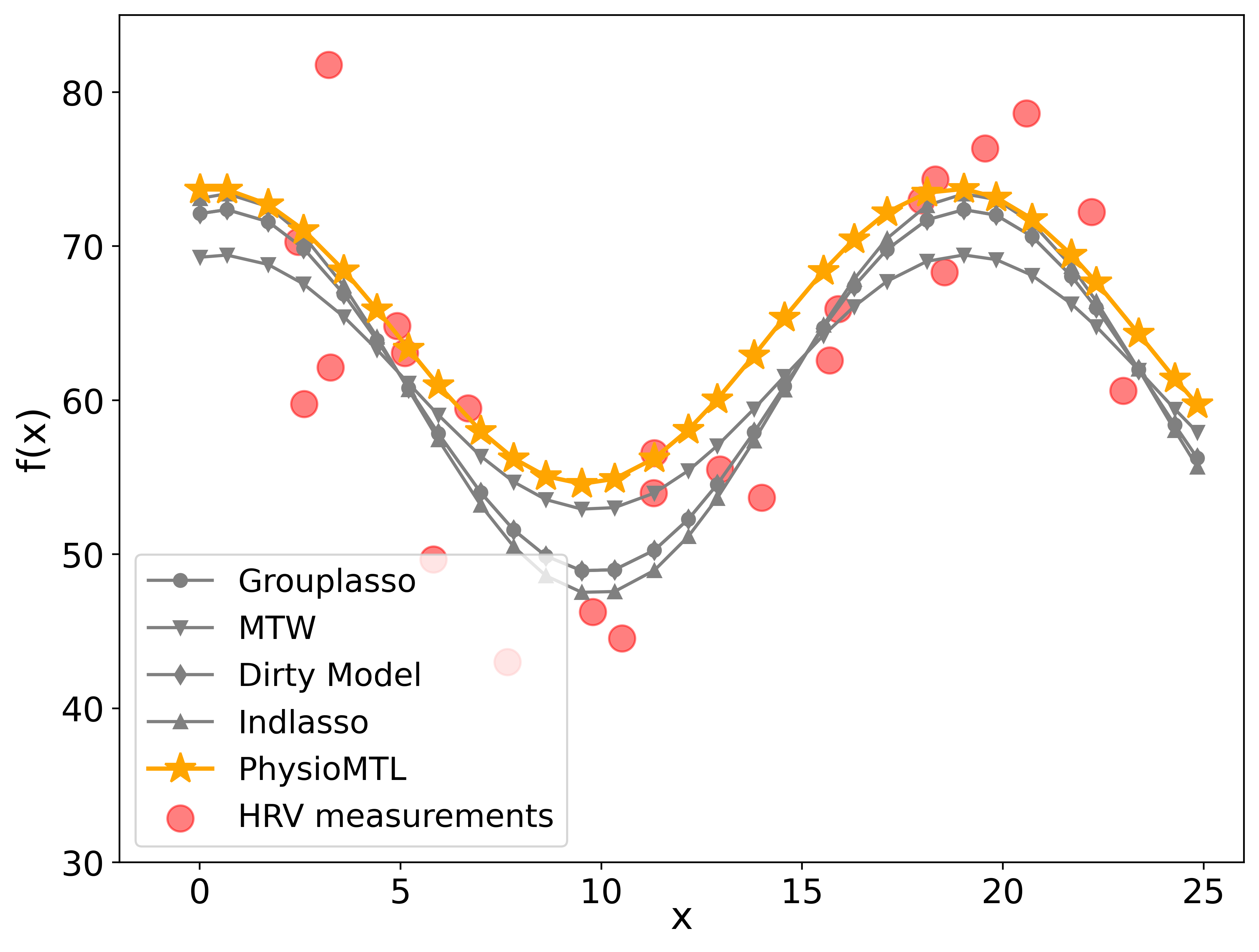
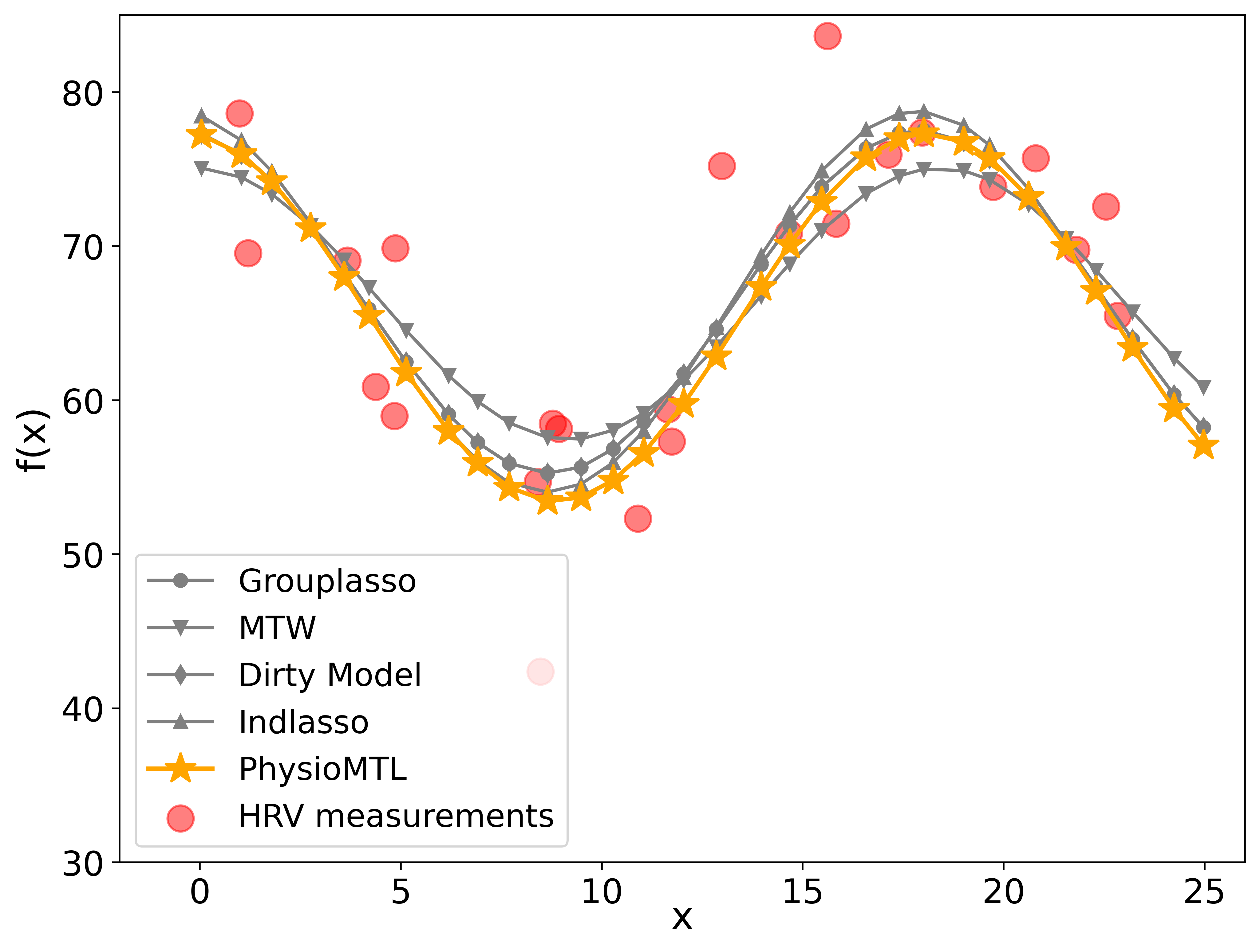
fig:uneven_app [Task 1] [Task 2] [Task 3] [Task 4] [Task 5]

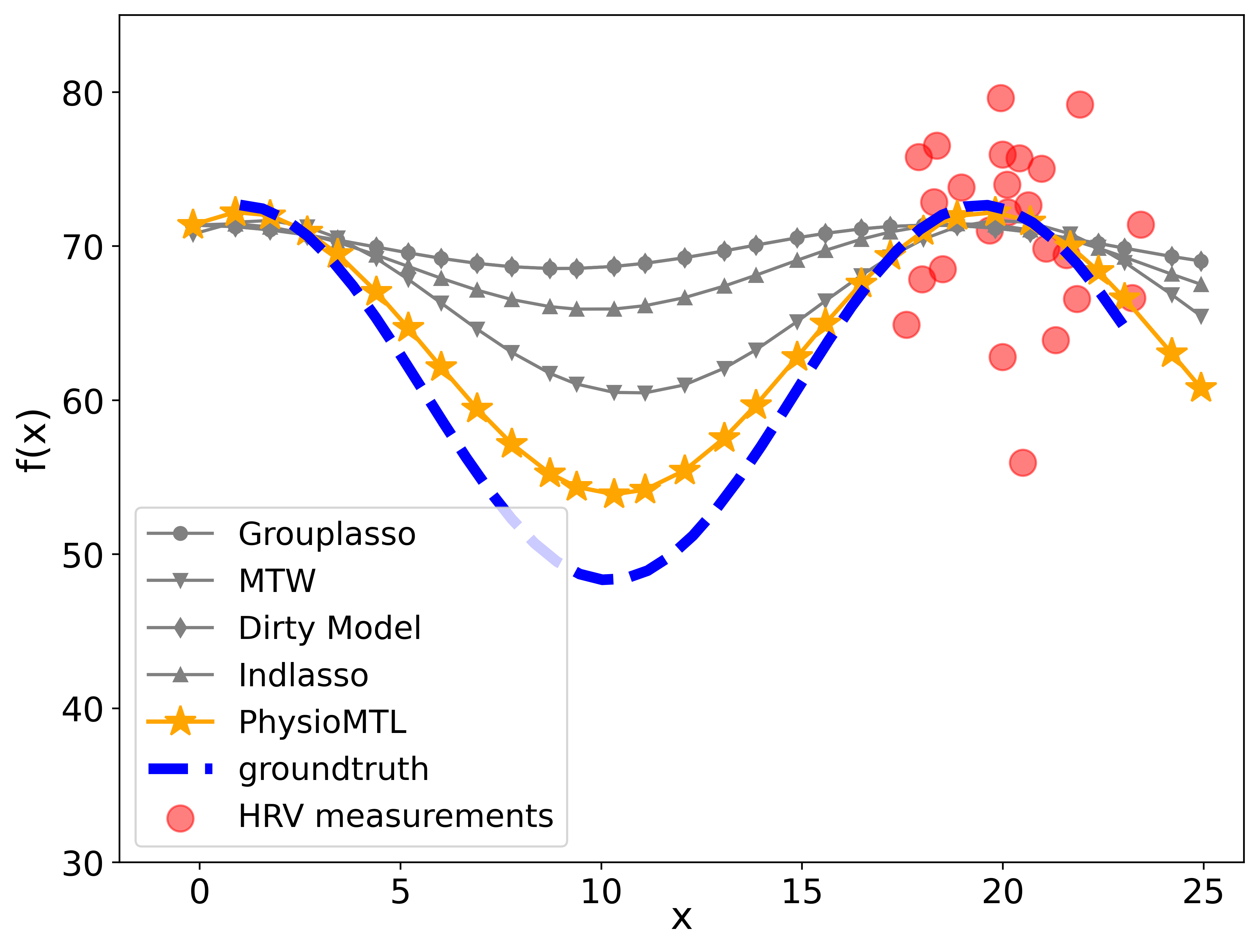
Figure 7: Here we overlay the regression results on a training set of 5 tasks where Task 5 is missing data from a significant portion of the domain.

C.2 MMASH

	Age	BMI	Activity	Sleep	Stress
Mean	26.95	23.11	0.43	6.55	35.57
Std	4.50	3.17	0.58	1.28	16.08
Min	20.0	19.41	0.00	4.40	14.00
25%	25.0	21.63	0.00	5.87	26.00
50%	27.0	22.84	0.25	6.50	32.00
75%	28.0	23.18	0.67	7.27	41.00
Max	40.0	33.24	2.00	10.50	74.00

Table 3: Descriptive statistics of all the demographic and lifestyle factors we use in the MMASH dataset.

fig:mmash_linear [Age] [BMI] [Activity]
[Sleep] [Stress] [Baseline]

Figure 8: The counterfactual analysis on the MMASH dataset using a linear transport map. We vary the attributes of a hypothetical subjective’s task-wise features and investigate the resulting HRV variational. Each feature investigated (age, BMI, activity, sleep, and stress) is continuous, however, for ease of visualization we vary each feature on a discrete grid.

C.3 AHMS

	Age	BMI	Activity	Sleep	VO2max
Mean	44.44	27.12	0.69	7.38	33.79
Std	12.32	5.86	0.43	0.87	8.48
Min	23.0	18.42	0.20	4.69	15.13
25%	35.0	23.09	0.45	6.95	26.90
50%	42.50	25.43	0.56	7.30	33.57
75%	52.25	30.00	0.79	7.97	39.28
Max	79.0	47.24	3.21	10.19	52.60

Table 4: Descriptive statistics of all the demographic and lifestyle factors we use in the AHMS dataset.

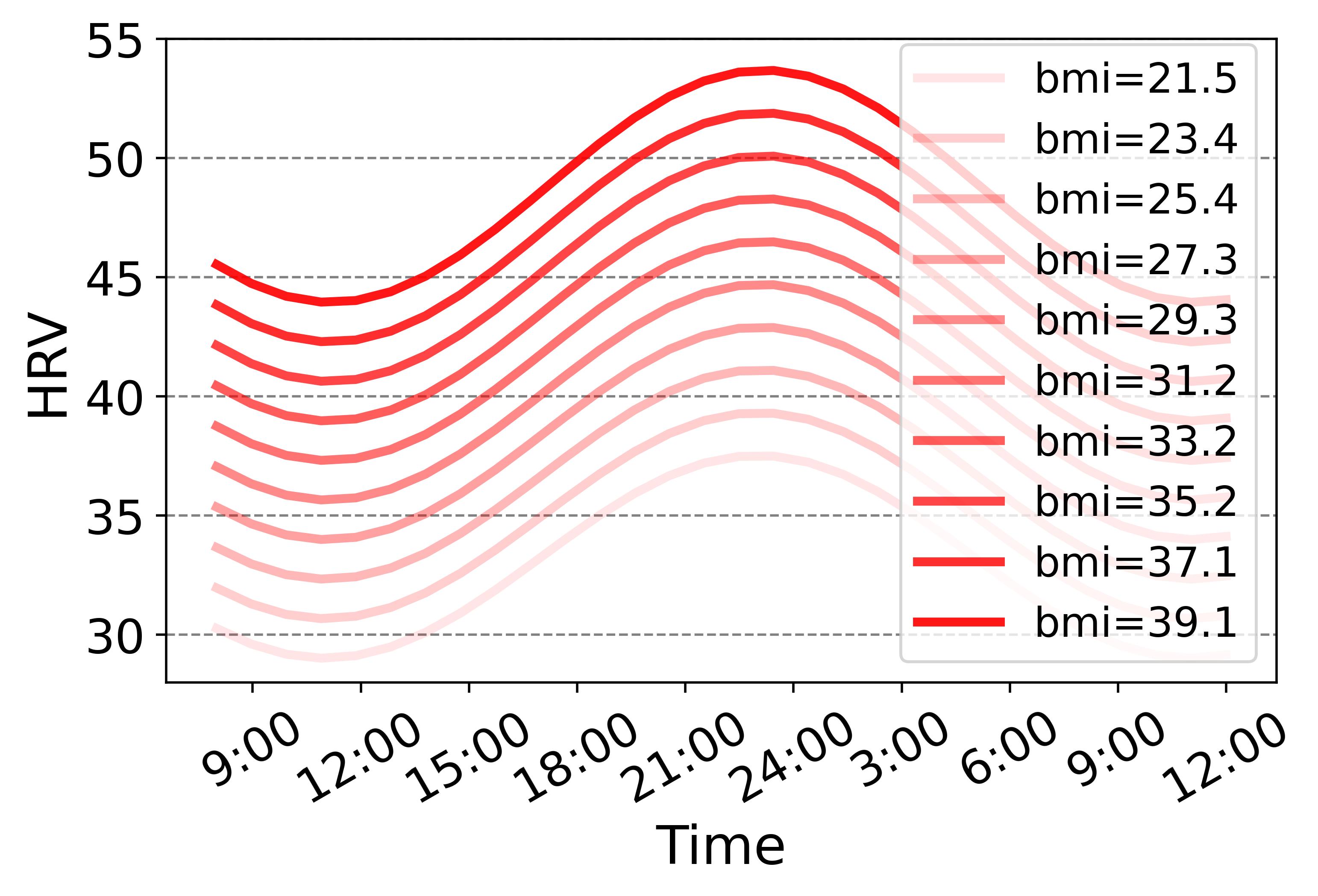
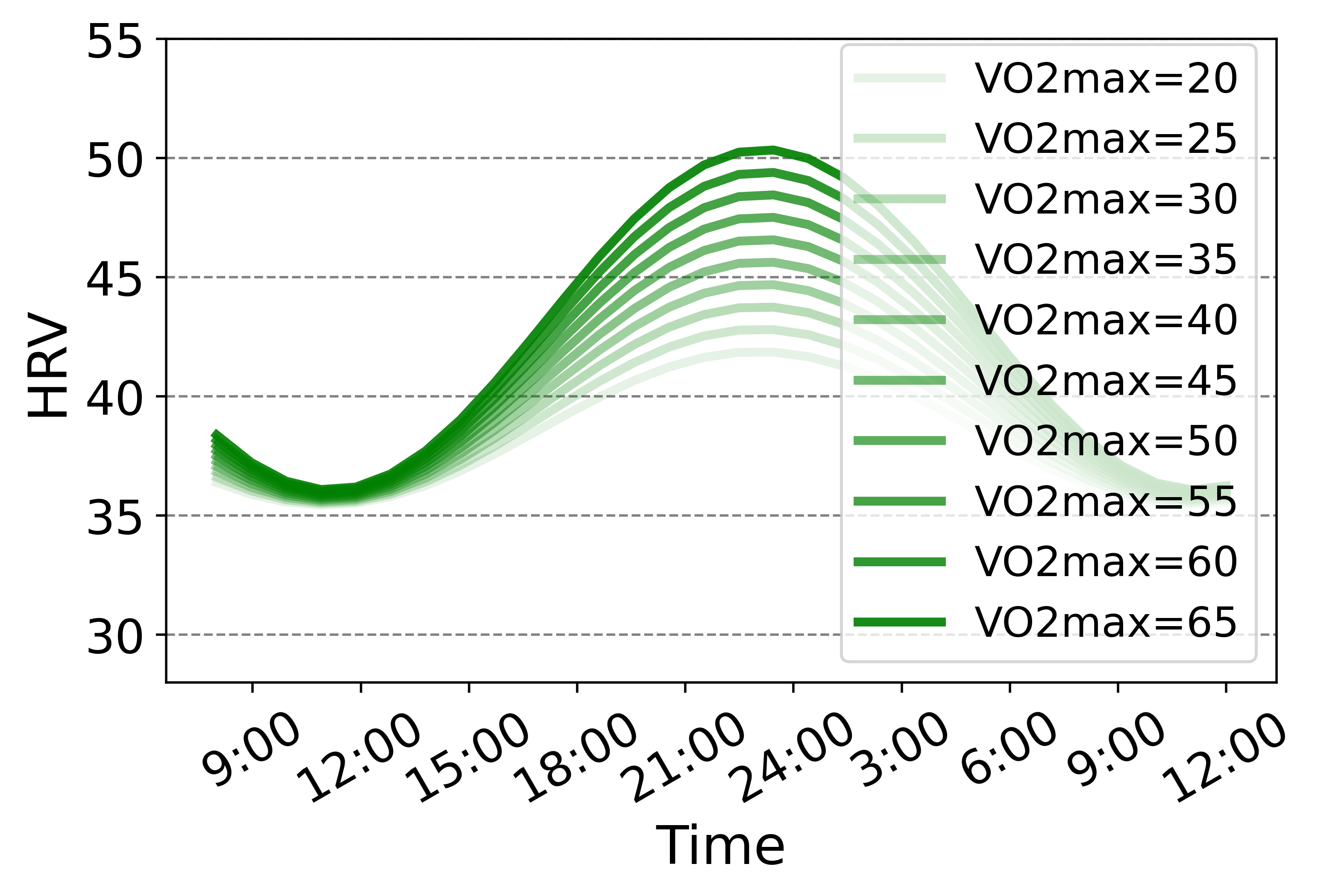
fig:ahms_linear [Age] [BMI] [Activity]
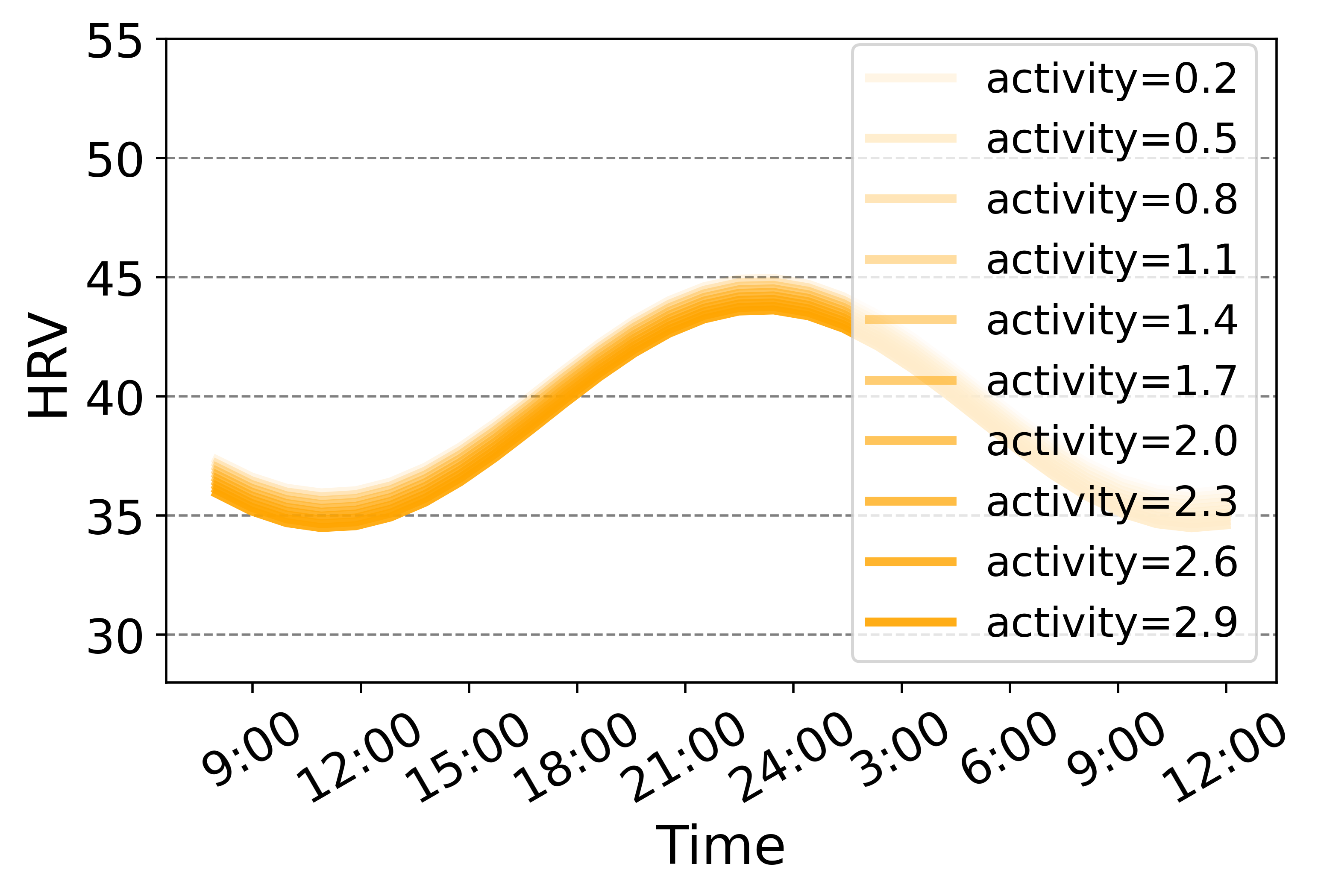
[Sleep] [VO2_max] [Baseline]

Figure 9: The counterfactual analysis on the AHMS dataset using a linear transport map. We vary the attributes of a hypothetical subjective’s task-wise features and investigate the resulting HRV variational. Each feature investigated (age, BMI, activity, sleep, and VO2_max) is continuous, however, for ease of visualization we vary each feature on a discrete grid.

References

- Abhishekh et al. (2013) Hulegar A Abhishekh, Palgun Nisarga, Ravikiran Kisan, Adoor Meghana, Sajish Chandran, Trichur Raju, and Talakad N Sathyaprabha. Influence of age and gender on autonomic regulation of heart. Journal of clinical monitoring and computing, 27(3):259–264, 2013.
- Acharya et al. (2006) U Rajendra Acharya, K Paul Joseph, Natarajan Kannathal, Choo Min Lim, and Jasjit S Suri. Heart rate variability: a review. Medical and biological engineering and computing, 44(12):1031–1051, 2006.
- Akay (2000) Metin Akay. Nonlinear Biomedical Signal Processing Vol. II: Dynamic Analysis and Modeling. Wiley-IEEE Press, 2000.
- Akselrod et al. (1981) Solange Akselrod, David Gordon, F Andrew Ubel, Daniel C Shannon, A Clifford Berger, and Richard J Cohen. Power spectrum analysis of heart rate fluctuation: a quantitative probe of beat-to-beat cardiovascular control. science, 213(4504):220–222, 1981.
- Akselrod et al. (1985) Solange Akselrod, David Gordon, Jeffrey B Madwed, Nancy C Snidman, Danied C Shannon, and Richard J Cohen. Hemodynamic regulation: investigation by spectral analysis. American Journal of Physiology-Heart and Circulatory Physiology, 249(4):H867–H875, 1985.
- Alesiani et al. (2020) Francesco Alesiani, Shujian Yu, Ammar Shaker, and Wenzhe Yin. Towards interpretable multi-task learning using bilevel programming. arXiv preprint arXiv:2009.05483, 2020.
- Altini and Plews (2021) Marco Altini and Daniel Plews. What is behind changes in resting heart rate and heart rate variability? a large-scale analysis of longitudinal measurements acquired in free-living. Sensors, 21(23):7932, 2021.
- Alvarez-Melis et al. (2019) David Alvarez-Melis, Stefanie Jegelka, and Tommi S Jaakkola. Towards optimal transport with global invariances. In The 22nd International Conference on Artificial Intelligence and Statistics, pages 1870–1879. PMLR, 2019.
- Apple (2019) Apple. Apple heart & movement study. https://clinicaltrials.gov/ct2/show/NCT04198194, 2019. ClinicalTrials.gov Identifier: NCT04198194.
- Astiz et al. (2019) Mariana Astiz, Isabel Heyde, and Henrik Oster. Mechanisms of communication in the mammalian circadian timing system. International journal of molecular sciences, 20(2):343, 2019.
- Berger et al. (1986) Ronald D Berger, Solange Akselrod, David Gordon, and Richard J Cohen. An efficient algorithm for spectral analysis of heart rate variability. IEEE Transactions on biomedical engineering, (9):900–904, 1986.
- Bickel et al. (2008) Steffen Bickel, Jasmina Bogojeska, Thomas Lengauer, and Tobias Scheffer. Multi-task learning for hiv therapy screening. In Proceedings of the 25th international conference on Machine learning, pages 56–63, 2008.
- Bonilla et al. (2007) Edwin V Bonilla, Felix V Agakov, and Christopher KI Williams. Kernel multi-task learning using task-specific features. In Artificial Intelligence and Statistics, pages 43–50. PMLR, 2007.
- Bowman et al. (2021) Clark Bowman, Yitong Huang, Olivia J Walch, Yu Fang, Elena Frank, Jonathan Tyler, Caleb Mayer, Christopher Stockbridge, Cathy Goldstein, Srijan Sen, et al. A method for characterizing daily physiology from widely used wearables. Cell reports methods, 1(4):100058, 2021.
- Carlier et al. (2020) Guillaume Carlier, Arnaud Dupuy, Alfred Galichon, and Yifei Sun. Sista: learning optimal transport costs under sparsity constraints. arXiv preprint arXiv:2009.08564, 2020.
- Chalmers et al. (2014) John A Chalmers, Daniel S Quintana, Maree J Abbott, Andrew H Kemp, et al. Anxiety disorders are associated with reduced heart rate variability: a meta-analysis. Frontiers in psychiatry, 5:80, 2014.
- Cheng et al. (2020) Li-Fang Cheng, Bianca Dumitrascu, Gregory Darnell, Corey Chivers, Michael Draugelis, Kai Li, and Barbara E Engelhardt. Sparse multi-output gaussian processes for online medical time series prediction. BMC medical informatics and decision making, 20(1):1–23, 2020.
- Christiani et al. (2021) Mark Christiani, Gregory J Grosicki, and Andrew A Flatt. Cardiac-autonomic and hemodynamic responses to a hypertonic, sugar-sweetened sports beverage in physically active men. Applied Physiology, Nutrition, and Metabolism, 46(10):1189–1195, 2021.
- Clifford and Tarassenko (2005) Gari D Clifford and Lionel Tarassenko. Quantifying errors in spectral estimates of hrv due to beat replacement and resampling. IEEE transactions on biomedical engineering, 52(4):630–638, 2005.
- Cuturi (2013) Marco Cuturi. Sinkhorn distances: Lightspeed computation of optimal transport. Advances in neural information processing systems, 26:2292–2300, 2013.
- De Boer et al. (1985) RW De Boer, JM Karemaker, and J Strackee. Relationships between short-term blood-pressure fluctuations and heart-rate variability in resting subjects i: a spectral analysis approach. Medical and biological engineering and computing, 23(4):352–358, 1985.
- Duru et al. (2000) Firat Duru, Reto Candinas, Gerald Dziekan, Ute Goebbels, Jonathan Myers, and Paul Dubach. Effect of exercise training on heart rate variability in patients with new-onset left ventricular dysfunction after myocardial infarction. American heart journal, 140(1):157–161, 2000.
- Electrophysiology (1996) Task Force of the European Society of Cardiology the North American Society of Pacing Electrophysiology. Heart rate variability: standards of measurement, physiological interpretation, and clinical use. Circulation, 93(5):1043–1065, 1996.
- Evgeniou and Pontil (2007) An Evgeniou and Massimiliano Pontil. Multi-task feature learning. Advances in neural information processing systems, 19:41, 2007.
- Finn et al. (2017) Chelsea Finn, Pieter Abbeel, and Sergey Levine. Model-agnostic meta-learning for fast adaptation of deep networks. In International Conference on Machine Learning, pages 1126–1135. PMLR, 2017.
- Genevay et al. (2019) Aude Genevay, Lénaic Chizat, Francis Bach, Marco Cuturi, and Gabriel Peyré. Sample complexity of sinkhorn divergences. In The 22nd International Conference on Artificial Intelligence and Statistics, pages 1574–1583. PMLR, 2019.
- Ghalwash et al. (2021) Mohamed Ghalwash, Zijun Yao, Prithwish Chakraporty, James Codella, and Daby Sow. Phenotypical ontology driven framework for multi-task learning. In Proceedings of the Conference on Health, Inference, and Learning, pages 183–192, 2021.
- Gower et al. (2004) John C Gower, Garmt B Dijksterhuis, et al. Procrustes problems, volume 30. Oxford University Press on Demand, 2004.
- Grzesiak et al. (2021) Emilia Grzesiak, Brinnae Bent, Micah T McClain, Christopher W Woods, Ephraim L Tsalik, Bradly P Nicholson, Timothy Veldman, Thomas W Burke, Zoe Gardener, Emma Bergstrom, et al. Assessment of the feasibility of using noninvasive wearable biometric monitoring sensors to detect influenza and the common cold before symptom onset. JAMA network open, 4(9):e2128534–e2128534, 2021.
- Hasty et al. (2021) Frederick Hasty, Guillermo García, Héctor Dávila, S Howard Wittels, Stephanie Hendricks, and Stephanie Chong. Heart rate variability as a possible predictive marker for acute inflammatory response in covid-19 patients. Military Medicine, 186(1-2):e34–e38, 2021.
- He et al. (2019) Xiao He, Francesco Alesiani, and Ammar Shaker. Efficient and scalable multi-task regression on massive number of tasks. In Proceedings of the AAAI Conference on Artificial Intelligence, volume 33, pages 3763–3770, 2019.
- Hirten et al. (2021) Robert P Hirten, Matteo Danieletto, Lewis Tomalin, Katie Hyewon Choi, Micol Zweig, Eddye Golden, Sparshdeep Kaur, Drew Helmus, Anthony Biello, Renata Pyzik, Alexander Charney, Riccardo Miotto, Benjamin S Glicksberg, Matthew Levin, Ismail Nabeel, Judith Aberg, David Reich, Dennis Charney, Erwin P Bottinger, Laurie Keefer, Mayte Suarez-Farinas, Girish N Nadkarni, and Zahi A Fayad. Use of physiological data from a wearable device to identify sars-cov-2 infection and symptoms and predict covid-19 diagnosis: Observational study. J Med Internet Res, 23(2):e26107, Feb 2021. ISSN 1438-8871. 10.2196/26107. URL https://www.jmir.org/2021/2/e26107.
- Hsieh and Tseng (2021) Ming-En Hsieh and Vincent Tseng. Boosting multi-task learning through combination of task labels-with applications in ecg phenotyping. In Proceedings of the AAAI Conference on Artificial Intelligence, volume 35, pages 7771–7779, 2021.
- Huikuri et al. (1994) Heikki V Huikuri, MJ Niemelä, Sirkku Ojala, Asko Rantala, MJ Ikäheimo, and KE Airaksinen. Circadian rhythms of frequency domain measures of heart rate variability in healthy subjects and patients with coronary artery disease. effects of arousal and upright posture. Circulation, 90(1):121–126, 1994.
- Jalali et al. (2010) Ali Jalali, Sujay Sanghavi, Chao Ruan, and Pradeep Ravikumar. A dirty model for multi-task learning. Advances in neural information processing systems, 23:964–972, 2010.
- Janati et al. (2019) Hicham Janati, Marco Cuturi, and Alexandre Gramfort. Wasserstein regularization for sparse multi-task regression. In The 22nd International Conference on Artificial Intelligence and Statistics, pages 1407–1416. PMLR, 2019.
- Janati et al. (2020) Hicham Janati, Thomas Bazeille, Bertrand Thirion, Marco Cuturi, and Alexandre Gramfort. Multi-subject meg/eeg source imaging with sparse multi-task regression. NeuroImage, 220:116847, 2020.
- Jarczok et al. (2013) Marc N Jarczok, Jian Li, Daniel Mauss, Joachim E Fischer, and Julian F Thayer. Heart rate variability is associated with glycemic status after controlling for components of the metabolic syndrome. International journal of cardiology, 167(3):855–861, 2013.
- Jarczok et al. (2019) Marc N Jarczok, Harald Guendel, Jennifer J McGrath, and Elisabeth M Balint. Circadian rhythms of the autonomic nervous system: Scientific implication and practical implementation. Chronobiology—The science of biological time structure, 2019.
- Kamath and Fallen (1993) Markad V Kamath and Ernest L Fallen. Power spectral analysis of heart rate variability: a noninvasive signature of cardiac autonomic function. Critical reviews in biomedical engineering, 21(3):245–311, 1993.
- Katona and Jih (1975) Peter G Katona and FELIX Jih. Respiratory sinus arrhythmia: noninvasive measure of parasympathetic cardiac control. Journal of applied physiology, 39(5):801–805, 1975.
- Kim et al. (2009) Ko Keun Kim, Jung Soo Kim, Yong Gyu Lim, and Kwang Suk Park. The effect of missing rr-interval data on heart rate variability analysis in the frequency domain. Physiological measurement, 30(10):1039, 2009.
- Koenig et al. (2014) Julian Koenig, MN Jarczok, M Warth, RJ Ellis, C Bach, TK Hillecke, and Julian Francis Thayer. Body mass index is related to autonomic nervous system activity as measured by heart rate variability—a replication using short term measurements. The journal of nutrition, health & aging, 18(3):300–302, 2014.
- Kumar et al. (2021) Agni Kumar, Vikramjit Mitra, Carolyn Oliver, Adeeti Ullal, Matt Biddulph, and Irida Mance. Estimating respiratory rate from breath audio obtained through wearable microphones. In 2021 43rd Annual International Conference of the IEEE Engineering in Medicine & Biology Society (EMBC), pages 7310–7315. IEEE, 2021.
- Li et al. (2021) Qian Li, Zhichao Wang, Shaowu Liu, Gang Li, and Guandong Xu. Causal optimal transport for treatment effect estimation. IEEE transactions on neural networks and learning systems, 2021.
- Li et al. (2011) Xian Li, Michele L Shaffer, Sol Rodriguez-Colon, Fan He, Deborah L Wolbrette, Peter Alagona, Chuntao Wu, and Duanping Liao. The circadian pattern of cardiac autonomic modulation in a middle-aged population. Clinical Autonomic Research, 21(3):143–150, 2011.
- Liu et al. (2019) Boyang Liu, Pang-Ning Tan, and Jiayu Zhou. Augmented multi-task learning by optimal transport. In Proceedings of the 2019 SIAM International Conference on Data Mining, pages 19–27. SIAM, 2019.
- Liu et al. (2014) Nehemiah T Liu, John B Holcomb, Charles E Wade, Mark I Darrah, and Jose Salinas. Utility of vital signs, heart rate variability and complexity, and machine learning for identifying the need for lifesaving interventions in trauma patients. Shock, 42(2):108–114, 2014.
- Liu et al. (2021) Wei Liu, Jie-Lin Qiu, Wei-Long Zheng, and Bao-Liang Lu. Comparing recognition performance and robustness of multimodal deep learning models for multimodal emotion recognition. IEEE Transactions on Cognitive and Developmental Systems, 2021.
- Lozano and Swirszcz (2012) Aurelie C Lozano and Grzegorz Swirszcz. Multi-level lasso for sparse multi-task regression. In Proceedings of the 29th International Coference on International Conference on Machine Learning, pages 595–602, 2012.
- Makkuva et al. (2020) Ashok Makkuva, Amirhossein Taghvaei, Sewoong Oh, and Jason Lee. Optimal transport mapping via input convex neural networks. In International Conference on Machine Learning, pages 6672–6681. PMLR, 2020.
- Manole et al. (2021) Tudor Manole, Sivaraman Balakrishnan, Jonathan Niles-Weed, and Larry Wasserman. Plugin estimation of smooth optimal transport maps. arXiv preprint arXiv:2107.12364, 2021.
- Murgia et al. (2019) Federico Murgia, Roberto Melotti, Luisa Foco, Martin Gögele, Viviana Meraviglia, Benedetta Motta, Alexander Steger, Michael Toifl, Daniel Sinnecker, Alexander Müller, et al. Effects of smoking status, history and intensity on heart rate variability in the general population: The chris study. PLoS One, 14(4):e0215053, 2019.
- Narin et al. (2018) Ali Narin, Yalcin Isler, Mahmut Ozer, and Matjaž Perc. Early prediction of paroxysmal atrial fibrillation based on short-term heart rate variability. Physica A: Statistical Mechanics and its Applications, 509:56–65, 2018.
- Nguyen et al. (2020) Tuan A Nguyen, Hyewon Jeong, Eunho Yang, and Sung Ju Hwang. Clinical risk prediction with temporal probabilistic asymmetric multi-task learning. arXiv preprint arXiv:2006.12777, 2020.
- Ni et al. (2019) Jianmo Ni, Larry Muhlstein, and Julian McAuley. Modeling heart rate and activity data for personalized fitness recommendation. In The World Wide Web Conference, pages 1343–1353, 2019.
- Nolte et al. (2017) Ilja M Nolte, M Loretto Munoz, Vinicius Tragante, Azmeraw T Amare, Rick Jansen, Ahmad Vaez, Benedikt Von Der Heyde, Christy L Avery, Joshua C Bis, Bram Dierckx, et al. Genetic loci associated with heart rate variability and their effects on cardiac disease risk. Nature communications, 8(1):1–17, 2017.
- Obozinski et al. (2006) Guillaume Obozinski, Ben Taskar, and Michael Jordan. Multi-task feature selection. Statistics Department, UC Berkeley, Tech. Rep, 2(2.2):2, 2006.
- Perrot et al. (2016) Michaël Perrot, Nicolas Courty, Rémi Flamary, and Amaury Habrard. Mapping estimation for discrete optimal transport. Advances in Neural Information Processing Systems, 29:4197–4205, 2016.
- Plews et al. (2014) Daniel J Plews, Paul B Laursen, Andrew E Kilding, and Martin Buchheit. Heart-rate variability and training-intensity distribution in elite rowers. Int J Sports Physiol Perform, 9(6):1026–1032, 2014.
- Pop et al. (2021) Gheorghe Nicusor Pop, Ruxandra Christodorescu, Dana Emilia Velimirovici, Raluca Sosdean, Miruna Corbu, Olivia Bodea, Mihaela Valcovici, and Simona Dragan. Assessment of the impact of alcohol consumption patterns on heart rate variability by machine learning in healthy young adults. Medicina, 57(9):956, 2021.
- Prosperi et al. (2020) Mattia Prosperi, Yi Guo, Matt Sperrin, James S Koopman, Jae S Min, Xing He, Shannan Rich, Mo Wang, Iain E Buchan, and Jiang Bian. Causal inference and counterfactual prediction in machine learning for actionable healthcare. Nature Machine Intelligence, 2(7):369–375, 2020.
- Qiu et al. (2018) Jie-Lin Qiu, Wei Liu, and Bao-Liang Lu. Multi-view emotion recognition using deep canonical correlation analysis. In International Conference on Neural Information Processing, pages 221–231. Springer, 2018.
- Qiu et al. (2022) Jielin Qiu, Jiacheng Zhu, Michael Rosenberg, Emerson Liu, and Ding Zhao. Optimal transport based data augmentation for heart disease diagnosis and prediction. arXiv preprint arXiv:2202.00567, 2022.
- Rangarajan et al. (1997) Anand Rangarajan, Haili Chui, and Fred L Bookstein. The softassign procrustes matching algorithm. In Biennial International Conference on Information Processing in Medical Imaging, pages 29–42. Springer, 1997.
- Romeo et al. (2020) Luca Romeo, Giuseppe Armentano, Antonio Nicolucci, Marco Vespasiani, Giacomo Vespasiani, and Emanuele Frontoni. A novel spatio-temporal multi-task approach for the prediction of diabetes-related complication: a cardiopathy case of study. In IJCAI, pages 4299–4305, 2020.
- Rossi et al. (2020) Alessio Rossi, Eleonora Da Pozzo, Dario Menicagli, Chiara Tremolanti, Corrado Priami, Alina Sîrbu, David A Clifton, Claudia Martini, and Davide Morelli. A public dataset of 24-h multi-levels psycho-physiological responses in young healthy adults. Data, 5(4):91, 2020.
- Rossi. et al. (2020) Alessio Rossi., Da Pozzo E., Menicagli D., Tremolanti C., Primai C., Sirbu A., Clifton D., Martini C., and Morelli D. Multilevel Monitoring of Activity and Sleep in Healthy People: (version 1.0.0). 2020. Link:https://doi.org/10.13026/cerq-fc86.
- Rothschild et al. (1988) Marylee Rothschild, Armand Rothschild, and Michael Pfeifer. Temporary decrease in cardiac parasympathetic tone after acute myocardial infarction. The American journal of cardiology, 62(9):637–639, 1988.
- Ruder (2017) Sebastian Ruder. An overview of multi-task learning in deep neural networks. arXiv preprint arXiv:1706.05098, 2017.
- Seguy et al. (2017) Vivien Seguy, Bharath Bhushan Damodaran, Rémi Flamary, Nicolas Courty, Antoine Rolet, and Mathieu Blondel. Large-scale optimal transport and mapping estimation. arXiv preprint arXiv:1711.02283, 2017.
- Shaffer and Ginsberg (2017) Fred Shaffer and Jay P Ginsberg. An overview of heart rate variability metrics and norms. Frontiers in public health, page 258, 2017.
- Shahnawaz and Dawood (2021) Muhammad Bilal Shahnawaz and Hassan Dawood. An effective deep learning model for automated detection of myocardial infarction based on ultrashort-term heart rate variability analysis. Mathematical Problems in Engineering, 2021, 2021.
- Shi et al. (2019) Manhong Shi, Chaoying Zhan, Hongxin He, Yanwen Jin, Rongrong Wu, Yan Sun, and Bairong Shen. Renyi distribution entropy analysis of short-term heart rate variability signals and its application in coronary artery disease detection. Frontiers in physiology, 10:809, 2019.
- Shui et al. (2019) Changjian Shui, Mahdieh Abbasi, Louis-Émile Robitaille, Boyu Wang, and Christian Gagné. A principled approach for learning task similarity in multitask learning. arXiv preprint arXiv:1903.09109, 2019.
- (76) Dimitris Spathis, Ignacio Perez-Pozuelo, Soren Brage, Nicholas J Wareham, and Cecilia Mascolo. Towards unsupervised wearable representations for longitudinal cardio-fitness prediction.
- Spathis et al. (2021) Dimitris Spathis, Ignacio Perez-Pozuelo, Soren Brage, Nicholas J Wareham, and Cecilia Mascolo. Self-supervised transfer learning of physiological representations from free-living wearable data. In Proceedings of the Conference on Health, Inference, and Learning, pages 69–78, 2021.
- Stuart and Wolfram (2020) Andrew M Stuart and Marie-Therese Wolfram. Inverse optimal transport. SIAM Journal on Applied Mathematics, 80(1):599–619, 2020.
- Taye et al. (2020) Getu Tadele Taye, Han-Jeong Hwang, and Ki Moo Lim. Application of a convolutional neural network for predicting the occurrence of ventricular tachyarrhythmia using heart rate variability features. Scientific reports, 10(1):1–7, 2020.
- Tu et al. (2021) Ruibo Tu, Kun Zhang, Hedvig Kjellström, and Cheng Zhang. Optimal transport for causal discovery. In ICML 2021 workshop on the Neglected Assumptions in Causal Inference, 2021.
- Villani (2009) Cédric Villani. Optimal transport: old and new, volume 338. Springer, 2009.
- Voss et al. (2015) Andreas Voss, Rico Schroeder, Andreas Heitmann, Annette Peters, and Siegfried Perz. Short-term heart rate variability—influence of gender and age in healthy subjects. PloS one, 10(3):e0118308, 2015.
- Wang et al. (2021) Haoxiang Wang, Han Zhao, and Bo Li. Bridging multi-task learning and meta-learning: Towards efficient training and effective adaptation. arXiv preprint arXiv:2106.09017, 2021.
- Wang et al. (2020) Wenlin Wang, Hongteng Xu, Zhe Gan, Bai Li, Guoyin Wang, Liqun Chen, Qian Yang, Wenqi Wang, and Lawrence Carin. Graph-driven generative models for heterogeneous multi-task learning. In Proceedings of the AAAI Conference on Artificial Intelligence, volume 34, pages 979–988, 2020.
- West (2012) Bruce J West. Fractal physiology and chaos in medicine, volume 16. World Scientific, 2012.
- Yu et al. (2020) Shujian Yu, Francesco Alesiani, Ammar Shaker, and Wenzhe Yin. Learning an interpretable graph structure in multi-task learning. arXiv preprint arXiv:2009.05618, 2020.
- Yuan and Lin (2006) Ming Yuan and Yi Lin. Model selection and estimation in regression with grouped variables. Journal of the Royal Statistical Society: Series B (Statistical Methodology), 68(1):49–67, 2006.
- Zhang et al. (2016) Dongfeng Zhang, Weijing Wang, and Fang Li. Association between resting heart rate and coronary artery disease, stroke, sudden death and noncardiovascular diseases: a meta-analysis. Cmaj, 188(15):E384–E392, 2016.
- Zhang et al. (2021) Haoran Zhang, Natalie Dullerud, Laleh Seyyed-Kalantari, Quaid Morris, Shalmali Joshi, and Marzyeh Ghassemi. An empirical framework for domain generalization in clinical settings. In Proceedings of the Conference on Health, Inference, and Learning, pages 279–290, 2021.
- Zhang and Yang (2018) Yu Zhang and Qiang Yang. An overview of multi-task learning. National Science Review, 5(1):30–43, 2018.
- Zhou et al. (2011a) Jiayu Zhou, Jianhui Chen, and Jieping Ye. Clustered multi-task learning via alternating structure optimization. Advances in neural information processing systems, 2011:702, 2011a.
- Zhou et al. (2011b) Jiayu Zhou, Jianhui Chen, and Jieping Ye. Malsar: Multi-task learning via structural regularization. Arizona State University, 21, 2011b.
- Zhou et al. (2011c) Jiayu Zhou, Lei Yuan, Jun Liu, and Jieping Ye. A multi-task learning formulation for predicting disease progression. In Proceedings of the 17th ACM SIGKDD international conference on Knowledge discovery and data mining, pages 814–822, 2011c.
- Zhu et al. (2021) Jiacheng Zhu, Aritra Guha, Mengdi Xu, Yingchen Ma, Rayleigh Lei, Vincenzo Loffredo, XuanLong Nguyen, and Ding Zhao. Functional optimal transport: Mapping estimation and domain adaptation for functional data. arXiv preprint arXiv:2102.03895, 2021.
- Zou and Hastie (2005) Hui Zou and Trevor Hastie. Regularization and variable selection via the elastic net. Journal of the royal statistical society: series B (statistical methodology), 67(2):301–320, 2005.