Quantum-enhanced Markov chain Monte Carlo

Abstract

Sampling from complicated probability distributions is a hard computational problem arising in many fields, including statistical physics, optimization, and machine learning. Quantum computers have recently been used to sample from complicated distributions that are hard to sample from classically, but which seldom arise in applications. Here we introduce a quantum algorithm to sample from distributions that pose a bottleneck in several applications, which we implement on a superconducting quantum processor. The algorithm performs Markov chain Monte Carlo (MCMC), a popular iterative sampling technique, to sample from the Boltzmann distribution of classical Ising models. In each step, the quantum processor explores the model in superposition to propose a random move, which is then accepted or rejected by a classical computer and returned to the quantum processor, ensuring convergence to the desired Boltzmann distribution. We find that this quantum algorithm converges in fewer iterations than common classical MCMC alternatives on relevant problem instances, both in simulations and experiments. It therefore opens a new path for quantum computers to solve useful—not merely difficult—problems in the near term.

Quantum computers promise to solve certain computational problems much faster than classical computers. However, current quantum processors are limited by their modest size and appreciable error rates. Recent efforts to demonstrate quantum speedups have therefore focused on problems that are both classically hard and naturally suited to current quantum devices, like sampling from complicated—though not explicitly useful—probability distributions [1, 2, 3]. Here we introduce and experimentally demonstrate a quantum algorithm that is similarly well-suited to current devices, which samples from distributions that can be both complicated and useful: the Boltzmann distribution of classical Ising models.

A classical Ising model consists of $n$ variables $(s_{1},\dots,s_{n})=\boldsymbol{s}$ called spins that can take values $s_{j}=\pm 1$ independently [4]. A model instance is defined by coefficients $\{J_{jk}\}_{j>k=1}^{n}$ and $\{h_{j}\}_{j=1}^{n}$ called couplings and fields respectively, together with a temperature $T>0$. It is often represented as a graph, as in Figs. 1a-b. Each spin configuration $\boldsymbol{s}\in\{1,-1\}^{n}$ is assigned an energy

$$E(\boldsymbol{s})=-\sum_{j>k=1}^{n}J_{jk}s_{j}s_{k}-\sum_{j=1}^{n}h_{j}s_{j}$$ (1)

and a corresponding Boltzmann probability $\mu(\boldsymbol{s})=\frac{1}{\mathcal{Z}}e^{-E(\boldsymbol{s})/T}$, where the partition function $\mathcal{Z}=\sum_{\boldsymbol{s}}e^{-E(\boldsymbol{s})/T}$ ensures normalization. Sampling from $\mu$ is a common subroutine in many disparate applications, including in statistical physics, where it is used to compute thermal averages [5]; in machine learning, to train Boltzmann machines [6]; and in combinatorial optimization, as part of the famous simulated annealing algorithm [7]. Indeed, this sampling is often a computational bottleneck when $J_{jk}$ and $h_{j}$ have varying signs and follow no particular pattern. Eq. (1) typically defines a rugged energy landscape for such instances, informally termed spin glasses [8], with many local minima that can be far from one another in Hamming distance, as depicted in Fig. 1c. In the $T\rightarrow 0$ limit, sampling from $\mu$ amounts to minimizing $E(\boldsymbol{s})$, which is NP-hard for spin glasses [9]. For small but non-zero $T$, sampling from $\mu$ requires finding several of the lowest-energy configurations, which may be far apart, not just the ground configuration(s). This hard regime will be our main focus.

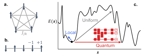
Figure 1: Ising model representations. a. Graph depicting an $n=5$ model instance where arrows (vertices) represent spins and edges represent the $\binom{n}{2}$ non-zero couplings $J_{jk}$. Fields $h_{j}$ are not shown. b. An $n=5$ model instance with only $n-1$ non-zero couplings. c. A rugged energy landscape typical of spin glasses, with the configurations $\boldsymbol{s}\in\{-1,1\}^{n}$ depicted in 1D. Typical proposed jumps for three MCMC algorithms, from a local minimum, are shown for illustration.

Markov chain Monte Carlo

Markov chain Monte Carlo (MCMC) is the most popular algorithmic technique for sampling from the Boltzmann distribution $\mu$ of Ising models in all of the aforementioned applications. In fact, it was named one of the ten most influential algorithms of the 20^th century in science and engineering [10]. It approaches the problem indirectly, without ever computing $\mu(\boldsymbol{s})$ and in turn the partition function $\mathcal{Z}$, which is believed to take $\Omega(2^{n})$ time. Rather, MCMC performs a sequence of random jumps between spin configurations, starting from a generic one and jumping from $\boldsymbol{s}$ to $\boldsymbol{s^{\prime}}$ with fixed transition probability $P(\boldsymbol{s^{\prime}}|\,\boldsymbol{s})$ in any iteration. Such a process is called a Markov chain. For it to form a useful algorithm, the transitions probabilities must be carefully chosen to make the process converge to $\mu$; that is, for the probability of being in $\boldsymbol{s}$ after many iterations to approach $\mu(\boldsymbol{s})$. Sufficient conditions for such convergence are that the Markov chain be irreducible and aperiodic (technical requirements that will always be met here [11]), and satisfy the detailed balance condition:

$$P(\boldsymbol{s^{\prime}}|\,\boldsymbol{s})\,\mu(\boldsymbol{s})=P(\boldsymbol{s}\,|\boldsymbol{s^{\prime}})\,\mu(\boldsymbol{s^{\prime}})$$ (2)

for all $\boldsymbol{s}\neq\boldsymbol{s^{\prime}}$ [12].

How to efficiently realize a $P$ satisfying these conditions? A powerful approach is to decompose each jump into two steps: Step 1 (proposal)- If the current configuration is $\boldsymbol{s}$, propose $\boldsymbol{s^{\prime}}$ with some probability $Q(\boldsymbol{s^{\prime}}|\,\boldsymbol{s})$. Step 2 (accept/reject)- Compute an appropriate acceptance probability $A(\boldsymbol{s^{\prime}}|\,\boldsymbol{s})$ based on $Q$ and $\mu$, then move to $\boldsymbol{s^{\prime}}$ with that probability (i.e., accept the proposal), otherwise remain at $\boldsymbol{s}$. This gives $P(\boldsymbol{s^{\prime}}|\,\boldsymbol{s})=A(\boldsymbol{s^{\prime}}|\,\boldsymbol{s})\,Q(\boldsymbol{s^{\prime}}|\,\boldsymbol{s})$ for all $\boldsymbol{s^{\prime}}\neq\boldsymbol{s}$. For a given $Q$ there are infinitely many choices of $A$ that satisfy detailed balance (2). One of the most popular is the Metropolis-Hastings (M-H) acceptance probability [13, 14]:

$$A(\boldsymbol{s^{\prime}}|\,\boldsymbol{s})=\min\left(1,\;\frac{\mu(\boldsymbol{s^{\prime}})}{\mu(\boldsymbol{s})}\frac{Q(\boldsymbol{s}\,|\boldsymbol{s^{\prime}})}{Q(\boldsymbol{s^{\prime}}|\,\boldsymbol{s})}\right).$$ (3)

Although $\mu(\boldsymbol{s})$ and $\mu(\boldsymbol{s^{\prime}})$ cannot be efficiently computed, Eq. (3) depends only on their ratio, which can be evaluated in $O(n^{2})$ time since $\mathcal{Z}$ cancels out. This cancellation underpins MCMC, and ensures that $A(\boldsymbol{s^{\prime}}|\,\boldsymbol{s})$ can be efficiently computed provided $Q(\boldsymbol{s}\,|\boldsymbol{s^{\prime}})/Q(\boldsymbol{s^{\prime}}|\,\boldsymbol{s})$ can too. The same is true for the other popular choice of $A$, called the Glauber or Gibbs sampler acceptance probability [11].

The most common way to propose a candidate $\boldsymbol{s^{\prime}}$ is by flipping ($s_{j}\!\mapsto\!-s_{j}$) a uniformly random spin $j\in[1,n]$ of the current configuration $\boldsymbol{s}$. We call this the local proposal strategy since $\boldsymbol{s}$ and $\boldsymbol{s^{\prime}}$ are always neighbors in terms of Hamming distance. The resulting acceptance probability can be computed efficiently, and the overall Markov chain converges quickly to $\mu$ for simple model instances at moderate $T$ [12]. Various non-local strategies can also be used (sometimes in combination [15]), including the uniform proposal strategy where $\boldsymbol{s^{\prime}}$ is picked uniformly at random from $\{-1,1\}^{n}$, and more complex ones which flip clusters of spins [16, 17, 18, 19]. Broadly, spin glasses at low $T$ present a formidable challenge for all of these approaches, manifesting in long autocorrelation, slow convergence, and ultimately long MCMC running times. This challenge is an active area of research due to the many applications in which it arises [20]. The problem: $\mu(\boldsymbol{s^{\prime}})/\mu(\boldsymbol{s})$ in Eq. (3), which comes from demanding detailed balance (2), is exponentially small in $\Delta E/T=[E(\boldsymbol{s^{\prime}})-E(\boldsymbol{s})]/T$ for energy-increasing proposals $\boldsymbol{s}\rightarrow\boldsymbol{s^{\prime}}$. Consequently, such proposals are frequently rejected. (And a rejected proposal still counts as an MCMC iteration.) This makes it difficult for Markov chains to explore rugged energy landscapes at low $T$, as they tend to get stuck in local minima for long stretches and to rarely cross large barriers in the landscape.

Quantum algorithm

To alleviate this issue, we introduce an MCMC algorithm which uses a quantum computer to propose moves and a classical computer to accept/reject them. It alternates between two steps: Step 1 (quantum proposal)- If the current configuration is $\boldsymbol{s}$, prepare the computational basis state ${|{\boldsymbol{s}}\rangle}$ on the quantum processor, where $s_{j}=\pm 1$ refers to an eigenvalue of $Z_{j}$. (E.g., if $\boldsymbol{s}=(1,1,-1)$, prepare ${|{\boldsymbol{s}}\rangle}={|{001}\rangle}$. We use $X_{j}$, $Y_{j}$ and $Z_{j}$ to denote $\sigma_{x}$, $\sigma_{y}$ and $\sigma_{z}$ on qubit $j$ respectively.) Then apply a unitary $U$ satisfying the symmetry constraint:

$$\big{|}{\langle{\boldsymbol{s^{\prime}}}|}U{|{\boldsymbol{s}}\rangle}\big{|}=\big{|}{\langle{\boldsymbol{s}}|}U{|{\boldsymbol{s^{\prime}}}\rangle}\big{|}\;\;\text{for all }\boldsymbol{s},\boldsymbol{s^{\prime}}\in\{-1,1\}^{n}.$$ (4)

Finally, measure each qubit in the $Z$ eigenbasis, i.e., the computational basis, denoting the outcome $\boldsymbol{s^{\prime}}$. Step 2 (classical accept/reject)- Compute $A(\boldsymbol{s^{\prime}}|\,\boldsymbol{s})$ from Eq. (3) on a classical computer and jump to $\boldsymbol{s^{\prime}}$ with this probability, otherwise stay at $\boldsymbol{s}$. While computing $Q(\boldsymbol{s^{\prime}}|\,\boldsymbol{s})$ and $Q(\boldsymbol{s}\,|\boldsymbol{s^{\prime}})$ may take exponential (in $n$) time in general, there is no need to do so: Eq. (3) depends only on their ratio, which equals 1 since $Q(\boldsymbol{s^{\prime}}|\,\boldsymbol{s})=|{\langle{\boldsymbol{s^{\prime}}}|}U{|{\boldsymbol{s}}\rangle}|^{2}=Q(\boldsymbol{s}\,|\boldsymbol{s^{\prime}})$ due to (4). This cancellation underpins our algorithm, and mirrors that between $\mu(\boldsymbol{s})$ and $\mu(\boldsymbol{s^{\prime}})$. The resulting Markov chain provably converges to the Boltzmann distribution $\mu$, but is hard to mimic classically, provided it is classically hard to sample the measurement outcomes of $U{|{\boldsymbol{s}}\rangle}$. This combination opens the possibility of a useful quantum advantage.

The symmetry requirement (4) ensures convergence to $\mu$, but does not uniquely specify $U$. Rather, we pick the quantum step of our algorithm heuristically with the aim of accelerating MCMC convergence in spin glasses at low $T$, while still satisfying condition (4). We then evaluate the resulting Markov chains through simulations and experiments. Several choices of $U$ are promising, including ones arising from quantum phase estimation and quantum annealing [11]. However, we focus here on evolution $U=e^{-iHt}$ under a time-independent Hamiltonian

$$H=(1-\gamma)\alpha\,H_{\text{prob}}+\gamma H_{\text{mix}}$$ (5)

for a time $t$, where

$$H_{\text{prob}}=-\!\!\sum_{j>k=1}^{n}J_{jk}Z_{j}Z_{k}-\sum_{j=1}^{n}h_{j}Z_{j}=\sum_{\boldsymbol{s}}E(\boldsymbol{s}){|{\boldsymbol{s}}\rangle}\!{\langle{\boldsymbol{s}}|}$$ (6)

encodes the classical model instance, $H_{\text{mix}}$ (discussed below) generates quantum transitions, and $\gamma\in[0,1]$ is a parameter controlling the relative weights of both terms. It is convenient to include a normalizing factor $\alpha=\|H_{\text{mix}}\|_{\textsc{f}}/\|H_{\text{prob}}\|_{\textsc{f}}$ in Eq. (5) so that both terms of $H$ share a common scale regardless of $\{J_{jk},h_{j}\}$, which can be arbitrary. ($\|M\|_{\textsc{f}}=\operatorname{tr}(M^{\dagger}M)^{1/2}$ is the Frobenius norm of a matrix $M$.)

In principle, $H_{\text{mix}}$ could comprise arbitrary weighted sums and products of $X_{j}$ and $Y_{j}Y_{k}$ terms. These produce a symmetric $H$ and therefore $U=U^{T}$ (although $U\neq U^{\dagger}$ generically), thus satisfying condition (4). If $H_{\text{mix}}$ were a dense matrix and $\gamma\ll 1$, a perturbative analysis shows that non-trivial quantum proposals $\boldsymbol{s}\rightarrow\boldsymbol{s^{\prime}}$ would exhibit a remarkable combination of features that suggest fast MCMC convergence [11]: Like local proposals, their absolute energy change $|\Delta E|=|E(\boldsymbol{s^{\prime}})-E(\boldsymbol{s})|$ is typically small, meaning they are likely to be accepted even if $\Delta E>0$. However, like uniform or cluster proposals, $\boldsymbol{s}$ and $\boldsymbol{s^{\prime}}$ are typically far in Hamming distance, so the resulting Markov chain can move rapidly between distant local energy minima. While a dense $H_{\text{mix}}$ would pose experimental difficulties, similar behavior is reported for various spin glasses in Refs. [21, 22, 23] using

$$H_{\text{mix}}=\sum_{j=1}^{n}X_{j}$$ (7)

and larger $\gamma$. Inspired by these results, we take Eq. (7) as the definition of $H_{\text{mix}}$ here. The normalizing factor $\alpha$ in Eq. (5) then takes the simple form

$$\alpha=\frac{\|H_{\text{mix}}\|_{\textsc{f}}}{\|H_{\text{prob}}\|_{\textsc{f}}}=\frac{\sqrt{n}}{\sqrt{\sum_{j>k=1}^{n}J_{jk}^{2}+\sum_{j=1}^{n}h_{j}^{2}}}$$ (8)

which—crucially—can be computed in $O(n^{2})$ time. Step 1 of our algorithm therefore consists of realizing quenched dynamics of a transverse-field quantum Ising model encoding the classical model instance, which can be efficiently simulated on a quantum computer [24]. Note, however, that our algorithm samples from a classical Boltzmann distribution $\mu$, not from a quantum Gibbs state as in Refs. [25, 26, 27, 28].

As an initial state ${|{\boldsymbol{s}}\rangle}$ evolves under $H$, it becomes delocalized due to $H_{\text{mix}}$ and effectively queries the classical energy function $E$ from Eq. (1) in quantum superposition through $H_{\text{prob}}$. The measurement outcome $\boldsymbol{s^{\prime}}$ is therefore influenced by the entire energy landscape. The details of this quantum evolution depend on the free parameters $\gamma$ and $t$. Rather than try to optimize these, we rely on a simple observation: instead of applying the same $U$ in every iteration of our algorithm, one could equally well pick $U$ at random in each iteration from an ensemble $\{U_{1},U_{2},\dots\}$ of unitaries, each satisfying condition (4). This amounts to sampling outputs from random circuits, initialized according to the state of a Markov chain. It is this randomized approach that we implement, by picking $\gamma$ and $t$ uniformly at random in each iteration [11], thus obviating the need to optimize these parameters. Note that we do not invoke adiabatic quantum evolution in any way, despite the familiar form of Eq. (5). Rather, the relative weights of $H_{\text{prob}}$ and $H_{\text{mix}}$ are held fixed throughout each quantum step.

Performance

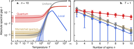
c. $\boldsymbol{\;\langle\delta\rangle\propto 2^{-kn}}$ fits Quantum $\color[rgb]{0,0,0}k=0.264(4)$ Mismatched $\color[rgb]{0.72265625,0.5703125,0.21484375}k=0.76(1)$ quantum Local $\color[rgb]{0.2549019607843137,0.4117647058823529,0.8823529411764706}k=0.94(4)$ Uniform $\color[rgb]{0.5019607843137255,0.5019607843137255,0.5019607843137255}k=0.948(7)$ Quantum enhancement factor in $k$: 3.6(1)

Figure 2: Average-case convergence rate simulations. The absolute spectral gap $\delta$, a measure of MCMC convergence rate, using the M-H acceptance probability (3) with different proposal strategies. All strategies were simulated classically. Lines/markers show the average $\delta$ over 500 random fully-connected Ising model instances for each $n$; error bands/bars show the standard deviation in $\delta$ over these instances. Dotted lines are for visibility. a. The slow-down of each strategy at low $T$. For the local proposal strategy, $\delta\rightarrow 0$ also at high $T$ because an eigenvalue of its transition matrix approaches $-1$. This artifact can be easily be remedied by using a lazy chain or the Gibbs sampler acceptance probability; the same is not true at low $T$, however [11]. b. Problem size dependence, with least squares exponential fits to the average $\delta$, weighted by the standard error of the mean. c. The resulting fit parameters and the average quantum enhancement exponent, which is the ratio of $k$ for the quantum algorithm and the smallest $k$ among classical proposal strategies (the local strategy, here). Uncertainties are from the fit covariance matrices. Similar data for different $n$ and $T$, model connectivity, and acceptance probabilities is shown in [11].

We now analyze the running time of our quantum algorithm through its convergence rate. MCMC convergence is inherently multifaceted. However, a Markov chain’s convergence rate is often summarized by its absolute spectral gap, $\delta\in[0,1]$, where the extremes of $\delta=0$ and $1$ describe the slowest and fastest possible convergence, respectively. This quantity is found by forming the transition probabilities $P(\boldsymbol{s^{\prime}}|\,\boldsymbol{s})$ into a $2^{n}\times 2^{n}$ matrix and computing its eigenvalues $\{\lambda\}$, all of which satisfy $|\lambda|\leq 1$ and describe a facet of the chain’s convergence. The absolute spectral gap, $\delta=1-\max_{\lambda\neq 1}|\lambda|$, describes the slowest facet. More concretely, it bounds the mixing time $\tau_{\varepsilon}$, defined as the minimum number of iterations required for the Markov chain’s distribution to get within any $\varepsilon>0$ of $\mu$ in total variation distance, for any initial distribution, as [12]

$$\left(\delta^{-1}-1\right)\ln\left(\frac{1}{2\varepsilon}\right)\;\leq\;\tau_{\varepsilon}\;\leq\;\delta^{-1}\ln\left(\frac{1}{\varepsilon\,\min_{\boldsymbol{s}}\mu(\boldsymbol{s})}\right).$$ (9)

Since $\delta$ is the only quantity on either side of (9) that depends on the proposal strategy $Q$, it is a particularly good metric for comparing the convergence rate of our quantum algorithm with that of common classical alternatives. Because $\delta$ depends on the model instance and on $T$, not just on $Q$, we analyzed our algorithm’s convergence in two complementary ways: First, we simulated it on a classical computer for many instances to elucidate the average-case $\delta$. Second, we implemented it experimentally for illustrative instances and analyzed both the convergence rate and the mechanism underlying the speedup observed in simulations. (Note that computing $\delta$ is different—and much more demanding—than simply running MCMC.) We used the M-H acceptance probability (3) throughout, although this choice has little impact on the results [11]. Unlike previously proposed algorithms which prepare a quantum state encoding $\mu$, ours uses simple, shallow quantum circuits [29, 30, 31, 32, 33, 34, 35]. Its alternating quantum/classical structure means that quantum coherence need only be maintained in each repetition of Step 1, rather than over the whole algorithm [36, 37]. Moreover, it generates numerous samples per run, like a fully classical MCMC algorithm, rather than a single one. These features make it sufficiently well-suited to current quantum processors that we observed a quantum speedup experimentally on up to $n=10$ qubits.

Average-Case Performance

For the first part of the analysis, we generated 500 random spin glass instances on $n$ spins by drawing each $J_{jk}$ and $h_{j}$ independently from standard normal distributions. We did not explicitly fix any couplings $J_{jk}$ to zero; the random instances are therefore fully connected as in Fig. 1a. This ensemble is the archetypal Sherrington-Kirkpatrick model [38] (up to a scale factor) with random local fields, where the fields serve to break inversion symmetry and thus increase the complexity. For each instance, we explicitly computed all the transition probabilities $\{P(\boldsymbol{s^{\prime}}|\,\boldsymbol{s})\}$ and then $\delta$ as a function of $T$ for different proposal strategies $Q$. We then averaged $\delta$ over the model instances, and repeated this process for $3\leq n\leq 10$. The results describe the average MCMC convergence rate as a function of $n$ and $T$. Two illustrative slices are shown in Fig. 2, where $n$ and $T$ are held fixed in turn. At high $T$, where $\mu$ is nearly uniform, the uniform proposal produces a fast-converging Markov chain with $\delta$ near $1$, as shown in Fig. 2a. However, both the uniform and local proposals suffer a sharp decrease in $\delta$ at lower $T$. This slow-down is much less pronounced for our quantum algorithm, which gives a substantially better $\delta$ on average than either classical alternative for $T\lesssim 1$.

For all three proposal strategies, the average scaling of $\delta$ with $n$ at $T=1$ fits well to $\langle\delta\rangle\propto 2^{-kn}$, as shown in Fig. 2b. Our algorithm appears to give an average-case polynomial enhancement in $\delta$ over the local and uniform proposals based on the fitted values of $k$, shown in Fig. 2c. These values depend on $T$, but their ratios suggest a roughly cubic/quartic enhancement at low temperatures regardless of the exact $T$ [11]. Finally, to elucidate the source of this average-case quantum enhancement, we also computed $\delta$ for a mismatched quantum proposal strategy, where moves are proposed like in our algorithm, but based on the wrong energy landscape. That is, rather than explore the relevant $E$ defined by coefficients $\{J_{jk}\}$ and $\{h_{j}\}$ as in Eqs. (1) and (6), the mismatched quantum strategy uses the wrong coefficients $\{\tilde{J}_{jk}\}$ and $\{\tilde{h}_{j}\}$ (drawn randomly from the same distribution as $J_{jk}$ and $h_{j}$) in its quantum Hamiltonian and therefore explores the wrong energy landscape $\tilde{E}$ in Step 1. The resulting $\delta$ is comparable with that of the uniform proposal in Fig. 2. This suggests that the $\delta$ enhancement in our algorithm indeed arises from exploring the classical energy landscape $E$ in quantum superposition to propose moves.

Experimental Implementation

For the second part of the analysis we focus in on individual model instances, for which we implemented our quantum algorithm experimentally and analyzed it in more depth than is feasible for a large number of instances. We generated random model instances and picked illustrative ones whose lowest-$E$ configurations include several near-degenerate local minima—a central feature of spin glasses at larger $n$ which hampers MCMC at low $T$. We then implemented our quantum algorithm experimentally for these instances on ibmq_mumbai, a 27-qubit superconducting quantum processor, using Qiskit [39], an open-source quantum software development platform. (The Ising model $T$ has no relation to the processor’s physical temperature.) We approximated $U=e^{-iHt}$ on this device through a randomly-compiled second-order Trotter-Suzuki product formula [40, 24, 41] with up to 48 layers of pulse-efficient 2-qubit gates [42] acting on up to 5 pairs of qubits in parallel [11], and set $Q(\boldsymbol{s}\,|\boldsymbol{s^{\prime}})/Q(\boldsymbol{s^{\prime}}|\,\boldsymbol{s})=1$ in the acceptance probability. Unlike in the first part of the analysis, we restricted our focus to model instances where $J_{jk}=0$ for $|j-k|\neq 1$ as in Fig. 1b, in order to match the connectivity of qubits in the quantum processor for this initial demonstration. Simulations show that the average-case $\delta$ for such instances is qualitatively similar to Fig. 2 [11].

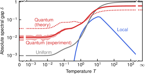
Figure 3: Convergence rate experiment. The absolute spectral gap $\delta$, a measure of MCMC convergence rate, for an illustrative model instance on $n=10$ spins with 1D connectivity. Each proposal strategy is combined with the M-H acceptance probability (3). To infer $\delta$ for the experimental realization of our algorithm, we recorded $5.76\times 10^{7}$ quantum transitions ${|{\boldsymbol{s}}\rangle}\rightarrow{|{\boldsymbol{s^{\prime}}}\rangle}$ between computational states with ${|{\boldsymbol{s}}\rangle}$ uniformly distributed, to estimate each $Q(\boldsymbol{s^{\prime}}|\,\boldsymbol{s})$. For each $T$, we used the full data set to estimate the MCMC transition matrix $P$ and in turn form a point estimate of $\delta$ (solid red line), then a random subsample of the data to compute 99% bootstrap confidence intervals (red error bands).

We focus on an $n=10$ model instance here in which the six lowest-$E$ configurations are all local minima, and the two lowest have an energy difference of just $|\Delta E|=0.05$. Similar instances with $n=8$ and $9$ are analyzed in [11]. For the present $n=10$ instance, $\delta$ closely follows the average in Fig. 2a for the local and uniform proposal strategies, as well as for our quantum algorithm in theory, as shown in Fig. 3. We estimated $\delta$ as a function of $T$ for the experimental realization of our quantum algorithm by counting quantum transitions ${|{\boldsymbol{s}}\rangle}\rightarrow{|{\boldsymbol{s^{\prime}}}\rangle}$ between all computational states ${|{\boldsymbol{s}}\rangle}$ and ${|{\boldsymbol{s^{\prime}}}\rangle}$ to estimate the MCMC transition matrix, which we then diagonalized. At low $T$, the inferred $\delta$ is smaller than the theoretical value due to experimental imperfections, but still significantly larger than that of either the local or uniform alternative. This constitutes an experimental quantum enhancement in MCMC convergence on current quantum hardware. At high $T$, the experimental $\delta$ is larger than the theoretical value for our quantum algorithm, which we attribute to noise in the quantum processor mimicking the uniform proposal to a degree. We also plot $\delta$ for common MCMC cluster algorithms (those of Swendsen-Wang, Wolff and Houdayer) in [11]. These are substantially more complicated than the local and uniform proposals, both conceptually and practically, but offer almost no $\delta$ enhancement in this setting compared to the simpler classical alternatives, so we do not focus on them here.

To further illustrate the increased convergence rate of our quantum-enhanced MCMC algorithm compared to these classical alternatives, we use it to estimate the average magnetization (with respect to the Boltzmann distribution $\mu$) of this same $n=10$ instance. The magnetization of a spin configuration $\boldsymbol{s}$ is $m(\boldsymbol{s})=\frac{1}{n}\sum_{j=1}^{n}s_{j}$, and the Boltzmann average magnetization is

$$\langle m\rangle_{\mu}=\sum_{\boldsymbol{s}}\mu(\boldsymbol{s})\,m(\boldsymbol{s}).$$ (10)

Eq. (10) involves a sum over all $2^{n}$ configurations, but given $N$ samples $\{\boldsymbol{s}\}=\mathcal{S}$ from $\mu$, the approximation $\langle m\rangle_{\mu}\approx N^{-1}\sum_{\boldsymbol{s}\in\mathcal{S}}m(\boldsymbol{s})$ can be accurate with high probability even if $N\ll 2^{n}$ [43]. While sampling from $\mu$ exactly may be infeasible, it is common to approximate $\langle m\rangle_{\mu}$ by the running average of $m(\boldsymbol{s})$ over MCMC trajectories (of one or several independent chains), and likewise for other average quantities. The quality of this approximation after a fixed number of MCMC iterations reflects the Markov chains’ convergence rate [12].

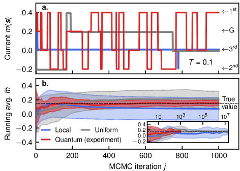
Figure 4: Magnetization estimate experiment. a. The current magnetization $m(\boldsymbol{s}^{(j)})$ for individual Markov chains after $j$ iterations. Each chain illustrates a different proposal strategy with uniformly random initialization. Arrows indicate the magnetization of the ground (G), 1^st, 2^nd and 3^rd excited configurations. b. Convergence of the running average $\bar{m}^{(j)}=\frac{1}{j}\sum_{k=0}^{j}m(\boldsymbol{s}^{(k)})$ from MCMC trajectories to the true value of $\langle m\rangle_{\mu}$ for different proposal strategies. For each strategy, the lines and error bands show the mean and standard deviation, respectively, of $\bar{m}^{(j)}$ over 10 independent chains. The inset depicts the same chains over more iterations. We do not use a burn-in period or thinning (i.e., the running average starts at $k=0$ and includes every iteration up to $k=j$), as these practices would introduce hyperparameters that complicate the interpretation. Both panels are for the same illustrative $n=10$ instance at $T=0.1$, and use the M-H acceptance probability (3).

We used this approach to estimate $\langle m\rangle_{\mu}$ at $T=0.1$ as shown in Fig. 4. At this temperature $\langle m\rangle_{\mu}\approx 0.15$, and the Boltzmann probabilities of the ground (i.e., lowest-$E$), 1^st, 2^nd and 3^rd excited configurations are approximately 43%, 26%, 19% and 12% respectively. This $T$ is therefore sufficiently high that sampling from $\mu$ is not simply an optimization problem (where $\langle m\rangle_{\mu}$ depends overwhelmingly on the ground configuration), but sufficiently low that $\langle m\rangle_{\mu}$ is mostly determined by a few low-$E$ configurations out of $2^{n}=1024$. Efficiently estimating $\langle m\rangle_{\mu}$ using MCMC therefore involves finding these configurations and—crucially—jumping frequently between them in proportion to their Boltzmann probabilities. The magnetization $m(\boldsymbol{s})$ for illustrative trajectories is shown in Fig. 4a for the local and uniform proposal strategies, and for an experimental implementation of our quantum algorithm. While each Markov chain finds a low-$E$ configurations quickly, our quantum algorithm jumps between these configurations noticeably faster than the others. The running average estimate for $\langle m\rangle_{\mu}$ from 10 independent Markov chains of each type is shown in Fig. 4b. Our quantum algorithm converges to the true value of $\langle m\rangle_{\mu}$, with no discernible bias, substantially faster than the two classical alternatives despite experimental imperfections.

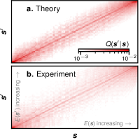
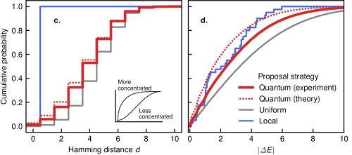
Figure 5: Quantum speedup mechanism. a. The classically-simulated probabilities of $\boldsymbol{s}\rightarrow\boldsymbol{s^{\prime}}$ proposals in our quantum algorithm, represented as a $2^{n}\times 2^{n}$ matrix whose columns are independent histograms. Both the initial and proposed configurations are sorted by increasing Ising energy $E$. b. The estimated proposal probabilities for our algorithm’s experimental realization. We estimated each $Q(\boldsymbol{s^{\prime}}|\,\boldsymbol{s})$ by the number of observed $\boldsymbol{s}\rightarrow\boldsymbol{s^{\prime}}$ proposals normalized by the number of $\boldsymbol{s}\rightarrow\text{[anything]}$ proposals, using a total of $5.76\times 10^{7}$ recorded quantum transitions. c. The probability distributions of Hamming distance between current ($\boldsymbol{s}$) and proposed ($\boldsymbol{s^{\prime}}$) configurations, for a uniformly random current configuration. That of the experiment uses the estimated probabilities from panel b, while the rest were computed exactly. d. The analogous distributions for $|\Delta E|=|E(\boldsymbol{s^{\prime}})-E(\boldsymbol{s})|$ of proposed jumps. Each distribution is depicted in full detail through its cumulative distribution function, with no binning. All panels are for the same illustrative $n=10$ model instance; none depend on $T$ or on the choice of acceptance probability.

Finally, we examined the mechanism underlying this observed quantum speedup. Recall that the local proposal strategy typically achieves small $|\Delta E|=|E(\boldsymbol{s^{\prime}})-E(\boldsymbol{s})|$ by picking $\boldsymbol{s^{\prime}}$ from the neighbors of $\boldsymbol{s}$, whereas the uniform proposal strategy typically picks $\boldsymbol{s^{\prime}}$ far from $\boldsymbol{s}$ at the cost of a larger $\Delta E$, as illustrated in Fig. 1c. Our quantum algorithm was motivated by the possibility of achieving the best of both: small $|\Delta E|$, and $\boldsymbol{s^{\prime}}$ far from $\boldsymbol{s}$. This combination of features is illustrated in Fig. 1c and borne out in Fig. 5. The proposal probabilities $Q(\boldsymbol{s^{\prime}}|\,\boldsymbol{s})$ arising in our algorithm for the same $n=10$ model instance are shown in Figs. 5a-b for theory and experiment respectively. Both show the same effect with good qualitative agreement: starting from $\boldsymbol{s}$, our quantum algorithm mostly proposes jumps to configurations $\boldsymbol{s^{\prime}}$ for which $|\Delta E|$ is small, even though $\boldsymbol{s}$ and $\boldsymbol{s^{\prime}}$ may be far in Hamming distance. This effect is especially pronounced between the lowest-$E$ configurations and also between highest-$E$ ones.

To further examine this effect we asked the following: for a uniformly random configuration $\boldsymbol{s}$, what is the probability of proposing a $\boldsymbol{s}\rightarrow\boldsymbol{s^{\prime}}$ jump for which $\boldsymbol{s}$ and $\boldsymbol{s^{\prime}}$ are separated by a Hamming distance $d$, or by an energy difference $|\Delta E|$? The resulting distributions are shown in Figs. 5c-d respectively for the local and uniform proposal strategies, as well as for the theoretical and experimental realizations of our quantum algorithm. The Hamming distance distribution for local proposals is concentrated at $d=1$ (by definition), whereas it is much more evenly spread for both uniform proposals and for our quantum algorithm, as shown in Fig. 5c. Conversely, the $\Delta E$ distribution of local proposals is more concentrated at small $\Delta E$ than that of uniform proposals. In theory, the corresponding distribution for our quantum algorithm is even more strongly concentrated at small $\Delta E$, as shown in Fig. 5d. The $\Delta E$ distribution from the experimental realization of our algorithm, however, lies between those of the local and uniform proposal strategies, due to experimental imperfections.

Outlook

Current quantum computers can sample from complicated probability distributions. We proposed and experimentally demonstrated a new quantum algorithm which leverages this ability in order to sample from the low-temperature Boltzmann distribution of classical Ising models, which is useful in many applications—not just complicated. Our algorithm uses relatively simple and shallow quantum circuits, thus enabling a quantum speedup on current hardware despite experimental imperfections. It works by alternating between quantum and classical steps on a shot-by-shot basis, unlike variational quantum algorithms, which typically run a quantum circuit many times in each step [44]. Rather, it uses a quantum computer to propose a random bit-string, which is accepted or rejected by a classical computer. The resulting Markov chain is guaranteed to converge to the desired Boltzmann distribution, even though it may not be possible to efficiently simulate classically. In this sense our algorithm is partially heuristic, like most classical MCMC algorithms: the eventual result is theoretically guaranteed, while fast convergence is established empirically.

Many state-of-the-art MCMC algorithms build upon simpler Markov chains in heuristically-motivated ways; for instance, by running several local M-H chains in parallel at different temperatures and occasionally swapping them [45, 18, 19]. Our quantum algorithm may provide a potent new ingredient for such composite algorithms in the near term. However, there remain ample opportunities for refinements and variations. For instance, a more targeted method of picking the parameters $\gamma$ and $t$ could further accelerate convergence [46]. Indeed, $t$ did not depend on the problem size $n$ in our implementation, although in some settings it should grow with $n$ if the qubits are all to remain within each others’ light cones. Moreover, different quantum processors with different connectivities, such as quantum annealers, may also be well-suited to implement our algorithm, perhaps without needing to discretize the Hamiltonian dynamics in Step 1.

Our algorithm is remarkably robust against imperfections. It achieves a speedup by proposing good jumps—but not every jump needs to be especially good for the algorithm to work well. (This is why picking $\gamma$ and $t$ at random works well: good values arise often enough.) For instance, if an error occurs in the quantum processor while a jump is being proposed, the proposal will be accepted/rejected as usual, and the Markov chain can still converge to the target distribution provided such errors do not break the $Q(\boldsymbol{s^{\prime}}|\,\boldsymbol{s})=Q(\boldsymbol{s}\,|\boldsymbol{s^{\prime}})$ symmetry on average [11]. Rather than produce the wrong result, we found that such errors merely slow the convergence at low $T$ by making our algorithm more classical. Indeed, in the limit of fully depolarizing noise, our algorithm reduces to MCMC with a uniform proposal. Our simulations suggest that the quantum speedup increases with the problem size $n$. However, we also expect the quantum noise to increase with $n$, in the absence of error correction, as the number of potential errors grows. The combined effect of these competing factors at larger $n$ is currently unknown. It is interesting to note, however, that the cubic/quartic speedup we observed, should it persist at larger $n$, might give a quantum advantage on a modest fault-tolerant quantum computer despite the error correction overhead [34, 47].

Characterizing our algorithm at larger scales will require different methods than those employed here. For instance, a Markov chain’s absolute spectral gap is a broad and unambiguous figure of merit, but it is not feasible to measure for large instances. This not an issue with our quantum algorithm in particular, but rather, with MCMC in general. Instead, a more fruitful approach may be to focus directly on how well our algorithm performs in various applications, such as in simulated annealing (for combinatorial optimization), for estimating thermal averages in many-body physics models, or for training and sampling from (classical) Boltzmann machines for machine learning applications.

Author Contributions

D.L. led the theory and the experiments. G.M., R.M., M.M. and P.W. contributed to the theory; in particular, D.L. and G.M. independently proposed a variant of this algorithm which uses quantum phase estimation, described in Section V-B of [11]. J.S.K., G.M., R.M., M.M. and S.S. contributed to the design of the experiments, and S.S. also contributed to their implementation. D.L. drafted the manuscript and supplemental material; all authors contributed to revising both.

References

- Arute et al. [2019] F. Arute, K. Arya, R. Babbush, D. Bacon, J. C. Bardin, R. Barends, R. Biswas, S. Boixo, F. G. Brandao, D. A. Buell, et al., Quantum supremacy using a programmable superconducting processor, Nature 574, 505 (2019).
- Wu et al. [2021] Y. Wu et al., Strong quantum computational advantage using a superconducting quantum processor, Phys. Rev. Lett 127, 180501 (2021).
- Zhong et al. [2021] H.-S. Zhong et al., Phase-programmable Gaussian boson sampling using stimulated squeezed light, Phys. Rev. Lett 127, 180502 (2021).
- Ising [1925] E. Ising, Beitrag zur Theorie des Ferromagnetismus, Z. Phys 31, 253 (1925).
- Huang [2008] K. Huang, Statistical mechanics (John Wiley & Sons, 2008).
- Ackley et al. [1985] D. H. Ackley, G. E. Hinton, and T. J. Sejnowski, A learning algorithm for Boltzmann machines, Cogn. Sci 9, 147 (1985).
- Kirkpatrick et al. [1983] S. Kirkpatrick, C. D. Gelatt, and M. P. Vecchi, Optimization by simulated annealing, Science 220, 671 (1983).
- Lucas [2014] A. Lucas, Ising formulations of many NP problems, Front. Phys 2 (2014).
- Barahona [1982] F. Barahona, On the computational complexity of Ising spin glass models, J. Phys. A 15, 3241 (1982).
- Dongarra and Sullivan [2000] J. Dongarra and F. Sullivan, Guest editors’ introduction to the top 10 algorithms, Comput. Sci. Eng 2, 22 (2000).
- [11] Supplemental Material.
- Levin and Peres [2017] D. Levin and Y. Peres, Markov Chains and Mixing Times, MBK (American Mathematical Society, 2017).
- Metropolis et al. [1953] N. Metropolis, A. W. Rosenbluth, M. N. Rosenbluth, A. H. Teller, and E. Teller, Equation of state calculations by fast computing machines, J. Comp. Phys. 21, 1087 (1953).
- Hastings [1970] W. K. Hastings, Monte Carlo sampling methods using Markov chains and their applications, Biometrika 57, 97 (1970).
- Andrieu et al. [2003] C. Andrieu, N. De Freitas, A. Doucet, and M. I. Jordan, An introduction to MCMC for machine learning, Mach. Learn 50, 5 (2003).
- Swendsen and Wang [1987] R. H. Swendsen and J.-S. Wang, Nonuniversal critical dynamics in Monte Carlo simulations, Phys. Rev. Lett 58, 86 (1987).
- Wolff [1989] U. Wolff, Collective Monte Carlo updating for spin systems, Phys. Rev. Lett 62, 361 (1989).
- Houdayer [2001] J. Houdayer, A cluster Monte Carlo algorithm for 2-dimensional spin glasses, Eur. Phys. J. B 22, 479 (2001).
- Zhu et al. [2015] Z. Zhu, A. J. Ochoa, and H. G. Katzgraber, Efficient cluster algorithm for spin glasses in any space dimension, Phys. Rev. Lett 115, 077201 (2015).
- Goodfellow et al. [2016] I. Goodfellow, Y. Bengio, and A. Courville, Deep Learning (MIT Press, 2016).
- Baldwin and Laumann [2018] C. L. Baldwin and C. R. Laumann, Quantum algorithm for energy matching in hard optimization problems, Phys. Rev. B 97, 224201 (2018).
- Smelyanskiy et al. [2020] V. N. Smelyanskiy, K. Kechedzhi, S. Boixo, S. V. Isakov, H. Neven, and B. Altshuler, Nonergodic delocalized states for efficient population transfer within a narrow band of the energy landscape, Phys. Rev. X 10, 011017 (2020).
- Smelyanskiy et al. [2019] V. N. Smelyanskiy, K. Kechedzhi, S. Boixo, H. Neven, and B. Altshuler, Intermittency of dynamical phases in a quantum spin glass, arXiv:1907.01609 (2019).
- Lloyd [1996] S. Lloyd, Universal quantum simulators, Science 273, 1073 (1996).
- Temme et al. [2011] K. Temme, T. J. Osborne, K. G. Vollbrecht, D. Poulin, and F. Verstraete, Quantum Metropolis sampling, Nature 471, 87 (2011).
- Yung and Aspuru-Guzik [2012] M.-H. Yung and A. Aspuru-Guzik, A quantum–quantum Metropolis algorithm, Proc. Natl. Acad. Sci 109, 754 (2012).
- Moussa [2019] J. E. Moussa, Measurement-based quantum Metropolis algorithm, arXiv:1903.01451 (2019).
- Wocjan and Temme [2021] P. Wocjan and K. Temme, Szegedy walk unitaries for quantum maps, arXiv preprint arXiv:2107.07365 (2021).
- Szegedy [2004] M. Szegedy, Quantum speed-up of Markov chain based algorithms, in 45th Annual IEEE Symposium on Foundations of Computer Science (2004) pp. 32–41.
- Richter [2007] P. C. Richter, Quantum speedup of classical mixing processes, Phys. Rev. A 76, 042306 (2007).
- Somma et al. [2008] R. D. Somma, S. Boixo, H. Barnum, and E. Knill, Quantum simulations of classical annealing processes, Phys. Rev. Lett. 101, 130504 (2008).
- Wocjan and Abeyesinghe [2008] P. Wocjan and A. Abeyesinghe, Speedup via quantum sampling, Phys. Rev. A 78, 042336 (2008).
- Harrow and Wei [2020] A. W. Harrow and A. Y. Wei, Adaptive quantum simulated annealing for Bayesian inference and estimating partition functions, in Proceedings of the Fourteenth Annual ACM-SIAM Symposium on Discrete Algorithms (SIAM, 2020) pp. 193–212.
- Lemieux et al. [2020] J. Lemieux, B. Heim, D. Poulin, K. Svore, and M. Troyer, Efficient quantum walk circuits for Metropolis-Hastings algorithm, Quantum 4, 287 (2020).
- Arunachalam et al. [2021] S. Arunachalam, V. Havlicek, G. Nannicini, K. Temme, and P. Wocjan, Simpler (classical) and faster (quantum) algorithms for Gibbs partition functions, in 2021 IEEE International Conference on Quantum Computing and Engineering (QCE) (IEEE, 2021) pp. 112–122.
- Wild et al. [2021a] D. S. Wild, D. Sels, H. Pichler, C. Zanoci, and M. D. Lukin, Quantum sampling algorithms for near-term devices, Phys. Rev. Lett. 127, 100504 (2021a).
- Wild et al. [2021b] D. S. Wild, D. Sels, H. Pichler, C. Zanoci, and M. D. Lukin, Quantum sampling algorithms, phase transitions, and computational complexity, Phys. Rev. A 104, 032602 (2021b).
- Sherrington and Kirkpatrick [1975] D. Sherrington and S. Kirkpatrick, Solvable model of a spin-glass, Phys. Rev. Lett 35, 1792 (1975).
- Anis Sajid et al. [2021] M. Anis Sajid et al., Qiskit: An open-source framework for quantum computing (2021).
- Suzuki [1985] M. Suzuki, Decomposition formulas of exponential operators and Lie exponentials with some applications to quantum mechanics and statistical physics, J. Math. Phys 26, 601 (1985).
- Wallman and Emerson [2016] J. J. Wallman and J. Emerson, Noise tailoring for scalable quantum computation via randomized compiling, Phys. Rev. A 94, 052325 (2016).
- Earnest et al. [2021] N. Earnest, C. Tornow, and D. J. Egger, Pulse-efficient circuit transpilation for quantum applications on cross-resonance-based hardware, Phys. Rev. Research 3, 043088 (2021).
- Ambegaokar and Troyer [2010] V. Ambegaokar and M. Troyer, Estimating errors reliably in Monte Carlo simulations of the Ehrenfest model, Am. J. Phys 78, 150 (2010).
- Cerezo et al. [2021] M. Cerezo, A. Arrasmith, R. Babbush, S. C. Benjamin, S. Endo, K. Fujii, J. R. McClean, K. Mitarai, X. Yuan, L. Cincio, et al., Variational quantum algorithms, Nat. Rev. Phys 3, 625 (2021).
- Swendsen and Wang [1986] R. H. Swendsen and J.-S. Wang, Replica Monte Carlo simulation of spin-glasses, Phys. Rev. Lett 57, 2607 (1986).
- Mazzola [2021] G. Mazzola, Sampling, rates, and reaction currents through reverse stochastic quantization on quantum computers, Phys. Rev. A 104, 022431 (2021).
- Babbush et al. [2021] R. Babbush, J. R. McClean, M. Newman, C. Gidney, S. Boixo, and H. Neven, Focus beyond quadratic speedups for error-corrected quantum advantage, PRX Quantum 2, 010103 (2021).