Modality Competition: What Makes Joint Training of Multi-modal Network Fail in Deep Learning? (Provably)

Abstract

Despite the remarkable success of deep multi-modal learning in practice, it has not been well-explained in theory. Recently, it has been observed that the best uni-modal network outperforms the jointly trained multi-modal network , which is counter-intuitive since multiple signals generally bring more information Wang et al. (2020). This work provides a theoretical explanation for the emergence of such performance gap in neural networks for the prevalent joint training framework. Based on a simplified data distribution that captures the realistic property of multi-modal data, we prove that for the multi-modal late-fusion network with (smoothed) ReLU activation trained jointly by gradient descent, different modalities will compete with each other. The encoder networks will learn only a subset of modalities. We refer to this phenomenon as modality competition. The losing modalities, which fail to be discovered, are the origins where the sub-optimality of joint training comes from. Experimentally, we illustrate that modality competition matches the intrinsic behavior of late-fusion joint training.

1 Introduction

Deep multi-modal learning has achieved remarkable performance in a wide range of fields, such as speech recognition Chan et al. (2016), semantic segmentation Jiang et al. (2018), and visual question-answering (VQA) Anderson et al. (2018). Intuitively, signals from different modalities often provide complementary information leading to performance improvement. However, Wang et al. (2020) observed that the best uni-modal network outperforms the multi-modal network obtained by joint training. Moreover, the analogous phenomenon has been noticed when using multiple input streams Goyal et al. (2017); Gat et al. (2020); Alamri et al. (2019).

Although deep multi-modal learning has become a critical practical machine learning approach, its theoretical understanding is quite limited. Some recent works have been proposed for understanding multi-modal learning from a theoretical standpoint Zhang et al. (2019); Huang et al. (2021); Sun et al. (2020); Du et al. (2021). Huang et al. (2021) provably argues that the generalization ability of uni-modal solutions is strictly sub-optimal than that of multi-modal solutions. Du et al. (2021) aims at identifying the reasons behind the surprising phenomenon of performance drop. Remarkably, these works have not analyzed what happened in the training process of neural networks, which we deem as crucial to understanding why naive joint training fails in practice. In particular, we state the fundamental questions that we address below and provably answer these questions by studying a simplified data model that captures key properties of real-world settings under the popular late-fusion joint training framework Baltrušaitis et al. (2018). We provide empirical results to support our theoretical framework. Our work is the first theoretical treatment towards the degenerating aspect of multi-modal learning in neural networks to the best of our knowledge.

1. How does the neural network encoder of each modality, trained by multi-modal learning, learn its feature representation?
2. Why does multi-modal learning in deep learning collapse in practice when naive joint training is applied?

1.1 Our Contributions

We study the multi-label classification task for a data distribution where each modality $\mathcal{M}_{r}$ is generated from a sparse coding model, which shares similarities with real scenarios (formally presented and explained in Section 2). Our data model for each modality owns a special structure called “insufficient data,” which represents cases where each modality alone cannot adequately predict the task. Such a structure is common in practical multi-modal applications Yang et al. (2015); Liu et al. (2018); Gat et al. (2020). Under this data model, we consider joint training based on late-fusion multi-modal network with one-layer neural network, activated by smoothed ReLU as modality encoder, and features from different modalities are passed to one-layer linear classifier after being fused by sum operation. Comparatively, the uni-modal network has similar pattern with the fusion operation eliminated. Both networks are trained by gradient descent (GD) over the multi-modal training set $\mathcal{D}$ or its uni-modal counterpart $\mathcal{D}^{r}$.

We analyze the optimization and generalization of multi and uni-network to probe the origin of the gap between theory and practice of multi-modal joint training in deep learning. Our key theoretical findings are summarized as follows.

• When only single modality is applied to training, the uni-modal network will focus on learning the modality-associated features, which leads to good performance (Theorem 5.1).

• When naive joint training is applied to the multi-modal network, the neural network will not efficiently learn all features from different modalities, and only a subset of modality encoders will capture sufficient feature representations (Theorem 5.2). We call this process “Modality Competition” and sketch its high-level idea below. During joint training, multiple modalities will compete with each other. Only a subset of modalities which correlate more with their encoding network’s random initialization will win and be learned by the final modality with other modalities failing to be explored.

• With the different feature learning process and the existence of insufficient structure, we further establish the theoretical guarantees for performance gap measured by test error, between the uni-modal and multi-modal networks (Corollary 5.3).

Empirical justification:

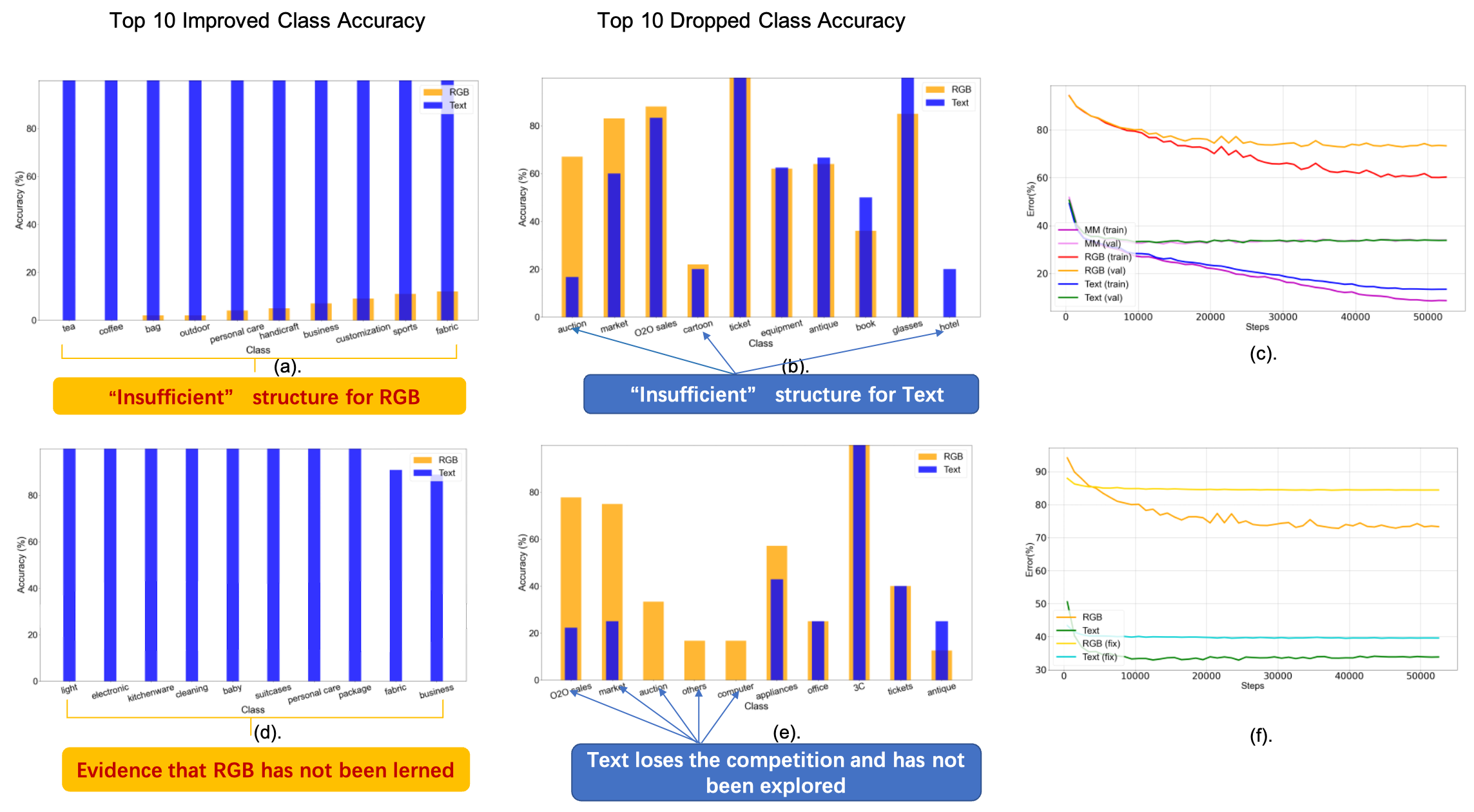
Figure 1: We experiment on item classification with the setups of image(RGB)-only, text-only, and multi-modality with joint training. Detailed setups are provided in Appendix C. (a) and (b) report the top $10$ classes based on the accuracy improvement and downgrade of text-only over image-only uni-model. (c) illustrates the training and validation error curves for text-only, image-only and text+image models. (d) and (e) demonstrate the similar comparison as (a) and (b) for the ones with a fixed encoder initialized by the multi-modal joint training. (f) illustrates the error curves for the directly trained uni-modal models and the ones with a fixed encoder.

We also support our findings with empirical results.

• For each modality, there exist certain classes where the corresponding uni-modal network has relatively low accuracy as shown in Figure 1 (a) and (b). For example, as demonstrated in Figure 1 (b), for text modality, while it predicts well on most classes, there exist some classes e.g. ”auction”, where it has low accuracy. Such observations verify the insufficient structure of uni-modal data.

• Figure 1 (c) supports the findings in Wang et al. (2020) that the best uni-modal outperforms the multi-modal.

• Only a subset of modalities learns good feature representations. As illustrated in Figure 1 (d), for some classes, e.g., “fabric”, “business” that were originally with slightly high accuracy (from (a)), the accuracy still drops to zero, which indicates that images are not learned for these classes in joint training. We have similar observations for text modality by comparing Figure 1 (b) and (e). Moreover, Figure 1 (f) shows that the feature representations obtained from joint training for each modality degrade compared to directly trained uni-modal.

The rest of the paper is organized as follows. We discuss the literature most related to our work in Section 2. In Section 4, we introduce the problem setup of our work. Main theoretical results are provided in Section 5. We present the main intuition and sketch of our proof in Section 6. We conclude our work and discuss some future work in Section 7.

2 Related Work

Success of multi-modal application.

With the development of deep learning, combining different modalities (text, vision, etc.) to solve the tasks has become a common approach in machine learning approach, and have demonstrated great power in various applications. Achievements have been made on tasks, which it is insufficient for single-modal models to learn, e.g., speech recognition Schneider et al. (2019); Dong et al. (2018), sound localization Zhao et al. (2019) and VQA Anderson et al. (2018). On the other hand, a large body of studies in vision & language learning Chen et al. (2020b); Li et al. (2020b, a); Lin et al. (2021) use pre-trained encoders to extract features from different modalities. These studies which demonstrate the success of multi-modal learning are beyond the scope of our research. Instead, in this paper, we focus on the end-to-end late-fusion multi-modal network with different modalities trained jointly and aim to theoretically explore the commonly observed phenomenon Wang et al. (2020) in this setting that multi-modal network does not make performance improvement over best uni-modal.

Theory of Multi-modal Learning

Theoretical progress in understanding multi-modal learning has lagged. Existing analysis for multi-view learning Xu et al. (2013); Amini et al. (2009); Federici et al. (2020), which is similar to multi-modal learning, does not readily generalize to multi-modal settings. It typically assumes that each view alone is sufficient to predict the target accurately, which is problematic in our settings, since in some cases we cannot make accurate decisions only with a single-modality (e.g., depth image for object detection Gupta et al. (2016)). One sequence of theoretical works try to explain the advantages of multi-modal using information-theoretical framework Sun et al. (2020) or assuming the training process is perfect Huang et al. (2021); Zhang et al. (2019). Recently, Du et al. (2021) utilized the easy-to-learn and paired features to explain the failure of joint training. However, their results do not take neural network architecture into consideration and do not provide the analysis of training process. Although these theoretical works shed great lights to the study of multi-modal learning, they have not yet given concrete mathematical answers to the fundamental questions we asked earlier.

Feature learning by neural networks.

In recent years, there has been an interest in studying the feature learning process of neural networks. Allen-Zhu and Li (2020c) contribute to understanding how ensemble and knowledge distillation work in deep learning based on a generic “multi-view” feature structure. Wen and Li (2021) prove that contrastive learning with proper data augmentation can learn desired sparse features resembling the features learning in supervised setting. Our proof techniques and intuitions are related to these recent literature, and our work studies a different perspective of feature learning by multi-modal joint training.

3 Notations

$[K]$ denotes the index set $\{1,\ldots,K\}.$ For a matrix $\mathbf{M}$, we use $\mathbf{M}_{j}$ to denote its $j$-th column. For a vector $x=(x_{1},\cdots,x_{d})^{\top}$, $\|x\|_{0}$ denotes the number of its non-zero elements and $\|x\|_{\infty}:=\max_{j\in d}|x_{j}|$. We use the standard big-O notation and its variants: $\mathcal{O}(\cdot),o(\cdot),\Theta(\cdot),\Omega(\cdot),\omega(\cdot)$, where $K$ is the problem parameter that becomes large. Occasionally, we use the symbol $\widetilde{\mathcal{O}}(\cdot)$ (and analogously with the other four variants) to hide $\operatorname{polylog}(K)$ factors. w.h.p means with probability at least $1-e^{-\Omega(\log^{2}(K))}$. $\textit{Supp}(\cdot)$ denotes the support of a random variable.

4 Problem Setup

We present our formulation, including the data distribution and learner network. We focus on a multi-class classification problem.

4.1 Data distribution:

Let $\mathbf{X}$ be a data sample and $y\in[K]$ be the corresponding label. For simplicity, we consider $\mathbf{X}:=(\mathbf{X}^{1},\mathbf{X}^{2})$ consisting of two modalities, and each modality $\mathcal{M}_{r}$, $r\in[2]$, is associated with a vector $\mathbf{X}^{r}\in\mathbb{R}^{d_{r}}$. We assume that the raw data is generated from a sparse coding model:

$$\mathbf{X}^{1}=\mathbf{M}^{1}z^{1}+\xi^{1},\quad \mathbf{X}^{2}=\mathbf{M}^{2}z^{2}+\xi^{2}$$

$$(z^{1},z^{2})\sim\mathcal{P}_{z}\quad \xi^{r}\sim\mathcal{P}_{\xi^{r}}\text{ for }r\in[2]$$

for dictionary $\mathbf{M}^{r}\in\mathbb{R}^{d_{r}\times K}$, where $z^{r}\in\mathbb{R}^{K}$ is the sparse vector and $\xi^{r}\in\mathbb{R}^{d_{r}}$ is the noise. There are three main components $\mathbf{M}^{r}$, $z^{r}$, $\xi^{r}$, and we will introduce them in detail below. For simplicity, we focus on the case where $\mathbf{M}^{1},\mathbf{M}^{2}$ are unitary with orthogonal columns.

Why sparse coding model?

Our data model shares many similarities with practical scenarios. Originated to explaining neuronal activation of human visual system Olshausen and Field (1997), sparse coding model has been widely used in machine learning applications to model different uni-modal data, such as image, text and audio Mairal et al. (2010); Yang et al. (2009); Yogatama et al. (2015); Arora et al. (2018); Whitaker and Anderson (2016); Grosse et al. (2012). Also, there is a line of research to develop sparse representations for multiple modalities simultaneously Yuan et al. (2012); Shafiee et al. (2015); Gwon et al. (2016).

In our following descriptions, we specify the choices for parameters including $\gamma_{r},s,\alpha$ for the sake of clarity. Our results apply to a wider range of parameters and generalized details are provided in Appendix A.1.

Distribution of sparse vector:

We generate $(z^{1},z^{2})$ from the joint distribution $\mathcal{P}_{z}$ as follows:

a). Select the label $y\in[K]$ uniformly at random;

b). Given the label $y$, the distribution $\mathcal{P}_{z^{r}\mid y}$ for each modality $\mathcal{M}_{r}$ is divided into two categories:

• With probability $\mu_{r}=\frac{1}{\mathrm{poly}(K)}$, $z^{r}$ is generated from the insufficient class:

  • $z^{r}_{y}=\Theta(\gamma_{r})$, we assume $\gamma_{1}=\gamma_{2}=\frac{1}{K^{0.05}}$.

  • For $j\neq y$, $z^{r}_{j}\in\{0\}\cup[\Omega(\rho_{r}),\rho_{r}]$ satisfying $\Pr(z^{r}_{j}\in[\Omega(\rho_{r}),\rho_{r}])=\frac{s}{K}$, where $s<K$ (we choose $s=K^{0.1}$) to control feature sparsity and $\rho_{r}=\frac{1}{\mathrm{polylog}(K)}$.

• With probability $1-\mu_{r}$, $z^{r}$ is generated from the sufficient class:

  • $z^{r}_{y}\in[1,C_{r}]$, where $C_{r}>1$ is a constant.

  • For $j\neq y$, $z^{r}_{j}\in\{0\}\cup[\Omega(1),c_{r}]$ satisfying $\Pr(z^{r}_{j}\in[\Omega(1),c_{r}])=\frac{s}{K}$ ,where $c_{r}$ is a constant $<\frac{1}{2}$.

In our settings, $\|z^{r}\|_{0}=\Theta(s)$ is a sparse vector. Each class $j$ has its associated feature $\mathbf{M}^{r}_{j}$ in each modality $\mathcal{M}_{r}$. We observe that for the sufficient class, the value of true label’s coordinate in $z^{r}$, i.e., $z^{r}_{y}$, is more significant than others. On the other hand, for the insufficient class, the target coordinate is smaller than the off-target signal in terms of order.

Significance of the insufficient class.

In practice, different modalities are of various importance under specific circumstance Ngiam et al. (2011); Liu et al. (2018); Gat et al. (2020). It is common that information from one single modality may be incomplete to build a good classifier Yang et al. (2015); Liu et al. (2018); Gupta et al. (2016). The restrictions on $z^{r}_{y}$ well capture this property, in the sense that there is a non-trivial probability $\mu_{r}$ that the coefficient $z^{r}_{y}$ is relatively small and easy to be concealed by the off-target signal. Therefore, when $z^{r}$ falls into this category, it provides insufficient information for the classification task. Given modality $\mathcal{M}_{r}$, we call $\mathbf{X}^{r}$ insufficient data if $z^{r}$ comes from the insufficient class, otherwise sufficient data. Our data model distinguishes the multi-modal learning from previous well-studied multi-view analysis, which assumes that each view is sufficient for classification Sridharan and Kakade (2008). Our classification is motivated by the distribution studied in Allen-Zhu and Li (2020c), where they utilize different levels of feature’s coefficient to model the missing of certain features.

Noise Model:

We allow the input to incorporate a general Gaussian noise plus feature noise, i.e.,

$$\xi^{r}={\xi^{r}}^{\prime}+\mathbf{M}^{r}\alpha^{r}$$

Here, the Gaussian noise ${\xi^{r}}^{\prime}\sim\mathcal{N}\left(0,\sigma_{g}^{2}\mathbf{I}_{d^{r}}\right)$. The spike noise $\alpha^{r}$ is any coordinate-wise independent non-negative random variable satisfying $\alpha_{y}^{r}=0$ and $\|\alpha^{r}\|_{\infty}\leq\alpha$ , where $\alpha>0$ is the strength of the feature noise. We consider $\alpha=\frac{1}{K^{0.6}}$.

Finally, we use $\mathcal{P}$ to denote the final data distribution of $(\mathbf{X},y)$, and the marginal distribution of $(\mathbf{X}^{r},y)$ is denoted by $\mathcal{P}^{r}$.

4.2 Learner Network

We present the learner networks for both multi-modal learning and uni-modal learning. To start, we first define a smoothed version of ReLU activation function.

Definition 4.1.

The smoothed ReLU function is defined as

$$\sigma(x)\stackrel{{\scriptstyle\text{ def }}}{{=}}\begin{cases}0&x\leq 0;\\ x^{q}/(\beta^{q-1}q)&x\in[0,\beta];\\ x-\beta\left(1-\frac{1}{q}\right)&x\geq\beta\end{cases}$$

where $q\geq 3$ is an integer and $\beta=\frac{1}{\mathrm{polylog}(K)}$.

Such activation function is utilized as a proxy to study the behavior of neural networks with ReLU activation in prior theoretical analysis Allen-Zhu and Li (2020c); Li et al. (2018); HaoChen et al. (2021); Woodworth et al. (2020), since it exhibits similar behaviour to the ReLU activation in the sense that $\sigma(\cdot)$ is linear when $x$ is large and becomes smaller when $x$ approaches zero. Moreover, it has desired property that the gradient of $\sigma(\cdot)$ is continuous. Besides, empirical studies illustrate that neural networks with polynomial activation have a matching performance compared to ReLU activation Allen-Zhu and Li (2020a).

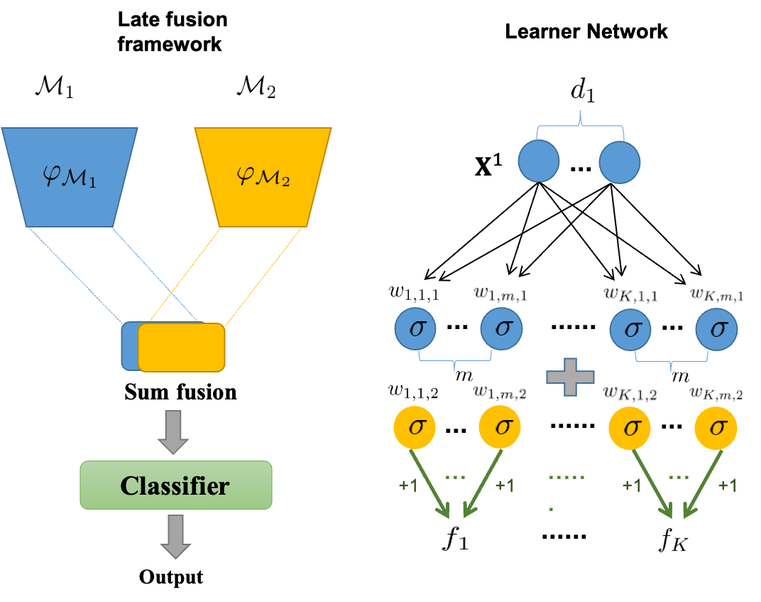
Figure 2: Late fusion framework and our learner network.

Multi-modal network:

We consider a late-fusion Wang et al. (2020) model on two modalities $\mathcal{M}_{1}$, and $\mathcal{M}_{2}$, which is illustrated by the left of Figure 2. Each modality is processed by a single-layer neural net $\varphi_{\mathcal{M}_{r}}:\mathbb{R}^{d_{r}}\rightarrow\mathbb{R}^{M}$ with smoothed ReLU activation $\sigma(\cdot)$, where $M$ is the number of neurons. Then their features are fused by sum operation and passed to a single-layer linear classifier $\mathcal{C}:\mathbb{R}^{M}\rightarrow\mathbb{R}^{K}$ to learn the target. We consider $M=K\cdot m$ with $m=\mathrm{polylog}(K)$. More precisely, as illustrated in Figure 2, the multi-modal network is formulated as follows:

$$f(\mathbf{X})=\left(f_{1}(\mathbf{X}),\ldots,f_{K}(\mathbf{X})\right)\in\mathbb{R}^{K},$$

$$f_{j}(\mathbf{X})=\sum^{m}_{l=1}\sigma(\langle w_{j,l,1},\mathbf{X}^{1}\rangle)+\sigma(\langle w_{j,l,2},\mathbf{X}^{2}\rangle)$$ (1)

where $w_{j,l,r}\in\mathbb{R}^{d_{r}}$ is the $(j-1)\cdot m+l$-th neuron of $\varphi_{m_{r}}$. Denote $\mathbf{W}^{r}$ the collection of weights $w_{j,l,r}$ and $\mathbf{W}^{r}_{j}:=(w_{j,1,r},\cdots,w_{j,m,r})^{\top}\in\mathbb{R}^{m\times d_{r}}$. Then the modality encoder of $\mathcal{M}_{r}$ can be written as:

$$\varphi_{\mathcal{M}_{r}}(\mathbf{W}^{r},\mathbf{X}^{r})=\left(\sigma({\mathbf{W}^{r}_{1}}^{\top}\mathbf{X}^{r}),\cdots\sigma({\mathbf{W}^{r}_{K}}^{\top}\mathbf{X}^{r})\right)$$

where $\sigma(\cdot)$ is applied element-wise. The classifier layer simply connects the entries from $(j-1)\cdot m+1$-th to $j\cdot m$-th to the $j$-th output $f_{j}(\cdot)$ with non-trainable weights all equal to $1$. The assumption that the second layer is fixed is common in previous works Du et al. (2018); Ji and Telgarsky (2019); Sarussi et al. (2021). Moreover, theoretical analysis in Huang et al. (2021) indicates that the success of multi-modal learning relies essentially on the learning of the hidden encoder layer. Nevertheless, we emphasize that our theory can easily adapt to the case where the second layer is trained.

Uni-modal network:

The network architecture of uni-modal is similar except that the fusion step is omitted. Mathematically, $f^{\text{uni},r}:\mathbb{R}^{d_{r}}\rightarrow\mathbb{R}^{K}$ is defined as follows:

$$f^{\text{uni},r}(\mathbf{X}^{r})=\left(f^{\text{uni},r}_{1}(\mathbf{X}^{r}),\ldots,f^{\text{uni},r}_{K}(\mathbf{X}^{r})\right)\in\mathbb{R}^{K},$$

$$f^{\text{uni},r}_{j}(\mathbf{X}^{r})=\sum^{m}_{l=1}\sigma(\langle\nu_{j,l,r},\mathbf{X}^{r}\rangle)$$ (2)

where $\nu_{j,l,r}\in\mathbb{R}^{d_{r}}$ denotes the weight. We use $\varphi^{\text{uni}}_{\mathcal{M}_{r}}$ to denote the modality encoder in uni-modal network.

Training data:

We are given $n$ multi-modal data pairs $\{\mathbf{X}_{i},y_{i}\}^{n}_{i=1}$ sampled from $\mathcal{P}$, denoted by $\mathcal{D}$. We use $\mathcal{D}^{r}$ to denote the uni-modal data pairs $\{\mathbf{X}^{r}_{i},y_{i}\}^{n}_{i=1}$ from $\mathcal{M}_{r}$. Moreover, we use $\mathcal{D}_{s}$ to denote the data pair that both $\mathbf{X}^{1}$ and $\mathbf{X}^{2}$ are sufficient data, and $\mathcal{D}_{i}$ to denote the data that at least one modality is insufficient. Denote the number of sufficient and insufficient data respectively as $n_{s}$ and $n_{i}$.

Training Algorithm:

We consider to learn the model parameter $\mathbf{W}$($\mathbf{W}^{r}$) by optimizing the empirical cross-entropy loss using gradient descent with learning rate $\eta>0$, which is a popular training combination investigated in the literature, e.g.,  Wang et al. (2020); Simonyan and Zisserman (2014).

• For multi-modal, the empirical loss is

  $$\mathcal{L}(f)=\frac{1}{n}\sum_{(\mathbf{X},y)\in\mathcal{D}}\mathcal{L}(f;\mathbf{X},y)$$ (3)

  where $\mathcal{L}(f;\mathbf{X},y)=-\log\frac{\exp(f_{y}(\mathbf{X}))}{\sum_{j\in[K]}\exp(f_{j}(\mathbf{X}))}$. We initialize $w^{(0)}_{j,l,r}\sim\mathcal{N}(0,\sigma^{2}_{0}\mathbf{I}_{d_{r}})$ where $\sigma_{0}=\frac{1}{\sqrt{K}}$. We use $f^{(t)}$ to denote the multi-modal network with $f$ with weights $\mathbf{W}^{(t)}$ at iteration $t$. The gradient descent update rule is:

  $$w_{j,l,r}^{(t+1)}=w_{j,l,r}^{(t)}-\eta\cdot\nabla_{w_{j,l,r}}\mathcal{L}(f^{(t)})$$

• Similarly, for uni-modal, the empirical loss and gradient update rule is defined as follows:

  $$\mathcal{L}(f^{\text{uni},r})=\frac{1}{n}\sum_{(\mathbf{X},y)\in\mathcal{D}^{r}}\mathcal{L}(f^{\text{uni},r};\mathbf{X}^{r},y)$$ (4)

  $$\nu_{j,l,r}^{(t+1)}=\nu_{j,l,r}^{(t)}-\eta\cdot\nabla_{\nu_{j,l,r}}\mathcal{L}({f^{\text{uni},r}}^{(t)})$$ (5)

  where $\mathcal{L}(f^{\text{uni},r};\mathbf{X}^{r},y)=-\log\frac{\exp(f^{\text{uni},r}_{y}(\mathbf{X}^{r}))}{\sum_{j\in[K]}\exp(f^{\text{uni},r}_{j}(\mathbf{X}^{r}))}$, and $\nu^{(0)}_{j,l,r}\sim\mathcal{N}(0,\sigma^{2}_{0}\mathbf{I}_{d_{r}})$.

5 Main Results

We present the main theorems of the paper here. We start with the optimization and generalization guarantees of the uni-modal network. Then, we study the feature learning process of multi-modal networks with joint training. We show that for naive joint training, each modality’s encoder has a non-trivial probability to learn unfavorable feature representations. Combining with the special structure of insufficient data, we immediately establish the performance gap between the best uni and multi-modal theoretically.

5.1 Uni-modal Network Results

The following theorem states that after enough iterations, the uni-modal networks can attain the global minimum of the empirical training loss, and such uni-modal solution also has a good test performance.

Theorem 5.1.

For every $r\in[2]$, for sufficiently large $K>0$ and every $\eta\leq\frac{1}{\operatorname{poly}(K)}$, after $T=\frac{\text{ poly }(K)}{\eta}$ many iteration, the learned uni-modal network ${f^{\text{uni},r}}^{(t)}$ w.h.p satisfies:

• Training error is zero:

  $$\frac{1}{n}\sum_{(\mathbf{X}^{r},y)\in\mathcal{D}^{r}}\mathbb{I}\left\{\exists j\neq y:\right.{f_{y}^{\text{uni},r}}^{(T)}(\mathbf{X}^{r})\leq\left.{f_{j}^{\text{uni},r}}^{(T)}(\mathbf{X}^{r})\right\}=0.$$

• The test error satisfies:

  $$\Pr_{(\mathbf{X}^{r},y)\sim\mathcal{P}^{r}}(\exists j\neq y:{f_{y}^{\text{uni},r}}^{(T)}(\mathbf{X}^{r})\leq{f_{j}^{\text{uni},r}}^{(T)}(\mathbf{X}^{r}))=(1\pm o(1))\mu_{r}$$

Recall that $\mu_{r}$ represents the proportion of data falling into the insufficient class for modality $\mathcal{M}_{r}$. Note that ${f^{\text{uni},r}}^{(T)}$ not only minimizes the training error, but the primary source of its test error is from the insufficient data that cannot provide enough feature-related information for the classification task. Therefore, Theorem 5.1 suggests that the uni-modal networks ${f^{\text{uni},r}}$ can learn ideal feature representations for the used single modality $\mathcal{M}_{r}$.

5.2 Multi-modal Network with Joint Training

In order to evaluate how good the feature representation learned by the encoder of each modality in joint training, we consider a uni-modal network ${f^{r}}^{(t)}:=\mathcal{C}(\varphi^{(t)}_{\mathcal{M}_{r}})$, where $\varphi^{(t)}_{\mathcal{M}_{r}}$ is the $\mathcal{M}_{r}$’s encoder learned by joint training at iteration $t$, and $\mathcal{C}$ is the non-trainable linear head we defined in Section 4.2. The input for ${f^{r}}^{(t)}$ is simply the data $\mathbf{X}^{r}$ from $\mathcal{M}_{r}$. We will measure the goodness of $\varphi^{(T)}_{\mathcal{M}_{r}}$ by the test performance of ${f^{r}}^{(T)}$, which is analogous to the method widely employed in empirical studies of self-supervised learning to evaluate the learned feature representations Chen et al. (2020a).

Theorem 5.2.

For sufficiently large $K>0$ and every $\eta\leq\frac{1}{\operatorname{poly}(K)}$, after $T=\frac{\text{ poly }(K)}{\eta}$ many iteration, for the multi-modal network $f^{(t)}$, ${f^{r}}^{(t)}:=\mathcal{C}(\varphi^{(t)}_{\mathcal{M}_{r}})$ w.h.p :

• Training error is zero:

  $$\frac{1}{n}\sum_{(\mathbf{X},y)\in\mathcal{D}}\mathbb{I}\{\exists j\neq y:f_{y}^{(T)}(\mathbf{X})\leq f_{j}^{(T)}(\mathbf{X})\}=0.$$

• For $r\in[2]$, with probability $p_{3-r}>0$, the test error of ${f^{r}}^{(T)}$ is high:

  $$\Pr_{(\mathbf{X}^{r},y)\sim\mathcal{P}^{r}}(\exists j\neq y:{f_{y}^{r}}^{(T)}(\mathbf{X}^{r})\leq{f_{j}^{r}}^{(T)}(\mathbf{X}^{r}))\geq\frac{1}{K}$$

  where $p_{1}+p_{2}=1-o(1)$, and $p_{r}\geq m^{-O(1)}$, $\forall r\in[2]$.

Discussion of $p_{r}$:

$p_{r}$ represents the probability that modality $\mathcal{M}_{3-r}$ fails to learn a good feature representation. The specific values of $p_{1}$ and $p_{2}$ are associated with the relative relation between the marginal distribution of $z^{1}$ and $z^{2}$ from sufficient class. Typically, if the lower bound of $\textit{Supp}(z^{r}_{y})$ is larger than the upper bound of $\textit{Supp}(z^{3-r}_{y})$, $p_{r}$ tends to be larger than $p_{3-r}$. Nevertheless, our results indicate that no matter how such relation varies, even in extreme cases (e.g., the lower bound of $\textit{Supp}(z^{r}_{y})$ is excessively larger than the upper bound of $\textit{Supp}(z^{3-r}_{y})$, both of $p_{1}$ and $p_{2}$ are lower bounded by a non-trivial value.

Feature representations learned in joint training are unsatisfactory.

From the optimization perspective, Theorem 5.2 shows that the multi-modal networks with joint training can be guaranteed to find a point that achieves zero error on the training set. However, such a solution is not optimal for both modalities. In particular, the output of the uni-modal network ${f^{r}}^{(T)}$, which we defined earlier to assess the quality of the learned modality encoder for $\mathcal{M}_{r}$, has a non-negligible probability to generalize badly and give a test error over $1/K$ (almost random guessing for $K$-classification, and exceedingly larger than ${f_{y}^{\text{uni},r}}^{(T)}$). The occurrence of such poor test performance indicates that w.h.p, at least one of the modality encoding networks learned relatively deficient knowledge about the modality-associated features.

Remark.

Originally, the intention of joint training is that for a multi-modal sample, if some of these modalities have insufficient structure, the information provided by remaining sufficient modalities can assist training and improve the accuracy. Nevertheless, Theorem 5.2 indicates that adding more modalities through naive joint possibly impairs the feature representation learning of the original modalities Consequently, the modal not only fails to exploit the extra modalities, but also loses the expertise of the original modality.

Based on the results in Theorem 5.2, we are able to characterize the performance gap between uni-modal and multi-modal with joint training in the following corollary.

Corollary 5.3 (Failure of Joint Training).

Suppose the assumptions in Theorem 5.2 holds, w.h.p, for joint training, the learned multi-modal network $f^{(T)}$ satisfies:

$$\Pr_{(\mathbf{X},y)\sim\mathcal{P}}(\exists j\neq y:f_{y}^{(T)}(\mathbf{X})\leq f_{j}^{(T)}(\mathbf{X}))\in[\sum_{r\in[2]}(p_{r}-o(1))\mu_{r},\sum_{r\in[2]}(p_{r}+o(1))\mu_{r}]$$

Combining with the results in Theorem 5.1, we immediately obtain:

$$\Pr_{(\mathbf{X},y)\sim\mathcal{P}}(\exists j\neq y: f_{y}^{(T)}(\mathbf{X})\leq f_{j}^{(T)}(\mathbf{X}))\geq\min_{r\in[2]}\Pr_{(\mathbf{X}^{r},y)\sim\mathcal{P}^{r}}(\exists j\neq y: {f_{y}^{\text{uni},r}}^{(T)}(\mathbf{X}^{r})\leq{f_{j}^{\text{uni},r}}^{(T)}(\mathbf{X}^{r}))$$

Notice that the test error of the joint training is approximately the weighted average of the test error of uni-modal network and is affected by two sets of factors $\{p_{r}\}_{r\in[2]}$, $\{\mu_{r}\}_{r\in[2]}$. The corollary has simple intuitive implications. If there exists a “strong” modality with a smaller $\mu_{r}$ (less insufficient structure) and a larger $p_{r}$ (more likely to prevail during training), the closer the joint training is to the best uni-modal, since the other modality is too weak to interfere the feature learning process of the strong modality.

6 Proof Outline

In this section we provide the proof sketch of our theoretical results. We provide overviews of multi-modal and uni-modal training process in Section 6.1 and 6.2 respectively, to provide intuitions for our proof. The complete proof is deferred to the supplementary.

6.1 Overview of the Joint Training Process

Given modality $\mathcal{M}_{r}$ and class $j\in[K]$, we characterize the feature learning of its modality encoder $\varphi_{\mathcal{M}_{r}}$ in the training process by quantity: $\Gamma^{(t)}_{j,r}=\max_{l\in[m]}[\langle\mathbf{M}^{r}_{j},w^{(t)}_{j,l,r}\rangle]^{+}.$ It can be seen that a larger $\Gamma^{(t)}_{j,r}$ implies better grasp of the target feature $\mathbf{M}^{r}_{j}$.

We will show that the training dynamics of multi-modal joint training can be decomposed into two phases: 1) Some special patterns of the neurons in the learner networks emerge and become singletons due to the random initialization, which demonstrates the phenomenon of modality competition; 2) As long as the neurons are activated by the winning modality, they will indeed converge to such modality, and ignore the other.

Phase 1: modality competition from random initialization.

Our proof begins by showing how the neurons in each modality encoder $\varphi_{\mathcal{M}_{r}}$ are emerged from random initialization. In particular, we will show that, despite the existence of multiple class-associated features (comes from different modalities), only one of them will be quickly learned by its corresponding encoding network, while the others will barely be discovered out of the random initialization. We call this phenomenon “modality competition” near random initialization, which demonstrates the origin of the sub-optimality of naive joint training.

Recall that at iteration $t=0$, the weights are initialized as $w_{j,l,r}^{(0)}\sim\mathcal{N}\left(0,\sigma_{0}^{2}\mathbf{I}_{d_{r}}\right)$. For $j\in[K]$, $r\in[2]$, define the following data-dependent parameter:

$$d_{j,r}(\mathcal{D})=\frac{1}{n\beta^{q-1}}\sum_{(\mathbf{X},y)\in\mathcal{D}_{s}}\mathbb{I}\{y=j\}\left(z^{r}_{j}\right)^{q}$$

Recall that $\mathcal{D}_{s}$ denotes the data pair that both $\mathbf{X}^{1}$ and $\mathbf{X}^{2}$ are sufficient data, i.e., the sparse vectors $z^{1}$ and $z^{2}$ both come from the sufficient class. Therefore, $d_{j,r}(\mathcal{D})$ represents the strength of the target signal for sufficient data from class $j$ and modality $\mathcal{M}$. Applying standard properties of the Gaussian distribution, we show the following critical property:

Property 6.1.

For each class $j\in[K]$, w.h.p, there exists $r_{j}\in[2]$, s.t.

$$\Gamma^{(0)}_{j,r_{j}}[d_{j,r_{j}}(\mathcal{D})]^{\frac{1}{q-2}}\geq\Gamma^{(0)}_{j,3-r_{j}}[d_{j,3-r_{j}}(\mathcal{D})]^{\frac{1}{q-2}}\cdot(1+\frac{1}{\operatorname{polylog}(K)})$$

In other words, by the property of random Gaussian initialization, for each class $j\in[K]$, there will be a $\mathcal{M}_{r_{j}}$, termed as winning modality, where the maximum correlation between $\mathbf{M}^{r_{j}}_{j}$ and one of the neurons of its corresponding encoder $\varphi_{\mathcal{M}_{r_{j}}}$ is slightly higher than the other modality $\mathcal{M}_{3-r_{j}}$. In our proof, we will identify the following phenomenon during the training: For every $j\in[K]$, at every iteration $t$, if $\mathcal{M}_{r_{j}}$ is the winning modality, then $\Gamma^{(t)}_{j,r_{j}}$ will grow faster than $\Gamma^{(t)}_{j,3-r_{j}}$. When $\Gamma^{(t)}_{j,r_{j}}$ reaches the threshold $\Theta(\beta)=\widetilde{\Theta}(1)$, $\Gamma^{(t)}_{j,3-r_{j}}$ still stucks at initial level around $\widetilde{O}(\sigma_{0})$.

Probability of winning.

Observing that $d_{j,r}(\mathcal{D})$ is related to the marginal distribution of $z^{r}$, we will prove that even in the extreme setting that $z_{j}^{r}\gg z_{j}^{3-r}$ for $j=y$ almost surely, which implies $d_{j,r}(\mathcal{D})\gg d_{j,3-r}(\mathcal{D})$ with high probability, $\mathcal{M}_{3-r}$ has a slightly notable probability, denoted by $p_{j,3-r}\geq m^{-O(1)}$, to be the winning modality for class $j$ out of random initialization. Noticing that $p_{j,r}$ also represents the probability that the modality $\mathcal{M}_{3-r}$ fails to be discovered for class $j\in[K]$ at the beginning, our subsequent analysis will illustrate that such a lag situation will continue, leading to bad feature representations for $\mathcal{M}_{3-r}$ with probability $p_{r}=\sum_{j\in[K]}p_{j,r}/K\geq m^{-O(1)}$.

Intuition:

Technically, in this phase, the activation function $\sigma(\cdot)$ is still in the polynomial or negative regime, and we can reduce the dynamic to tensor power method Anandkumar et al. (2015). We observe that the update of $\Gamma^{(t+1)}_{j,r}$ is approximately: $\Gamma^{(t+1)}_{j,r}\approx\Gamma^{(t)}_{j,r}+\eta\cdot A^{(t)}_{r}(\Gamma^{(t)}_{j,r})^{q-1}$, with $A^{(t)}_{r}=\Theta(1)$, which is similar to power method for $q$-th ($q\geq 3$) order tensor decomposition. By the behavior observed in randomly initialized tensor power method Anandkumar et al. (2015); Allen-Zhu and Li (2020c), a slight initial difference can create very dramatic growth gap. Based on this intuition, we introduce the Property 6.1 to characterize how much difference of initialization can make one of the modalities stand out to be the winning modality and propose the modality competition to further show that the neurons for the winning modality maintain the edge until they become roughly equal to $\Theta(\beta)=\widetilde{O}(1)$, while the others are still around initialization $\widetilde{O}(\sigma_{0})$ (recall that the networks are initialized by $\mathcal{N}(0,\sigma_{0}\mathbf{I}_{d_{r}})$).

Remark.

The idea that only part of modalities will win during the training is also motivated by a phenomenon called “winning the lottery ticket” identified in recent theoretical analysis for over-parameterized neural networks Li et al. (2020c); Wen and Li (2021); Allen-Zhu and Li (2020b). That is, for over-parameterized neural networks, only a small fraction of neurons has much larger norms than an average norm. Their works focus on who wins in the neural networks, while our focus is the winner of inputs, the modality.

Phase 2: converge to the winning modality.

The next phase of our analysis begins when one of the modalities already won the competition near random initialization, and focuses on showing that it will dominate until the end of the training. After the first phase, the pre-activation of the winning modality’s neurons will reach the linear region, while the pre-activation of the others still remain in the polynomial region or even negative. Yet, the loss starts to decrease significantly, and we prove that $\Gamma^{(t)}_{j,3-r_{j}}$ will no longer exceed $\widetilde{O}(\sigma_{0})$ until the training loss are close to converge. Therefore, the winning modality will remain the victory throughout the training.

6.2 Overview of the Uni-modal Training Process

The training process of uni-modal can also be decomposed into two phases, i.e., 1) learning the pattern, and 2) converging to the learned features. Similarly, we define $\Psi^{(t)}_{j,r}=\max_{l\in[m]}[\langle\mathbf{M}^{r}_{j},\nu^{(t)}_{j,l,r}\rangle]^{+}$ to quantify the feature learning for the uni-modal network $f^{\text{uni},r}$.

We briefly describe the difference between the uni-modal and the joint-training case. The main distinction arises from Phase 1. Intuitively, since there is only one predictive signal source without competitors, we prove that the network will focus on learning the features from the given modality in the first phase. In particular, $\Psi^{(t)}_{j,r}$ will grow fast to $\widetilde{O}(1)$ at the end of this phase. Then in Phase 2, the uni-modal will continue to explore the the learned patterns until the end of training.

7 Conclusions

In this paper, we provide novel theoretical understanding towards a qualitative phenomenon commonly observed in deep multi-modal applications, that the best uni-modal network outperforms the multi-modal network trained jointly under late-fusion settings. We analyze the optimization process and theoretically establish the performance gaps for these two approaches in terms of test error. In theory, we characterize the modality competition phenomenon to tentatively explain the main cause of the sub-optimality of joint training. Empirical results are provided to verify that our theoretical framework does coincide with the superior of the best uni-modal networks over joint training in practice. To a certain extent, our work reflects how the prevailing pre-training methods Lin et al. (2021), which are capable of extracting favorable features for every modality, lead to better performance for multi-modal learning. Our results also facilitate further theoretical analyses in multi-modal learning through a new mechanism that focuses on how modality encoder learns the features.

Appendix A Proofs for Multi-modal Joint Training

In this section, we will provide the proofs of Theorem 5.2 for multi-modal joint training. We will first focus on some properties and characterizations for modality at initialization. Our analysis actually rely on an induction hypothesis. Then we will introduce the hypothesis and prove that it holds in the whole training process. Finally, we will use this hypothesis to complete the proof of our main theorem.

A.1 Notations and Preliminaries

We first describe some preliminaries before diving into the proof.

Global Assumptions.

Throughout the proof in this section,

• We choose $\sigma_{0}^{q-2}=\frac{1}{K}$ for $q\geq 3$, where $\sigma_{0}$ controls the initialization magnitude.

• $m=\mathrm{polylog}(K)$, where $m$ controls the number of neurons.

• $\sigma_{g}=O(\sigma_{0}^{q-1})$, wehre $\sigma_{g}$ gives the magnitude of gaussian noise.

• $\alpha=\widetilde{O}(\sigma_{0})$, where $\alpha$ controls the feature noise.

• $\frac{s}{K}\leq\widetilde{O}(\sigma_{0})$, where $s$ controls the feature sparsity.

• $n_{i}\leq\frac{K^{2}\gamma^{q-1}}{s}$, where $n_{i}$ is the size of the insufficient multi-modal training data.

• $\rho_{r}=\frac{1}{\operatorname{poly}\log(K)}$ where $\rho_{r}$ control the off-target signal for insufficient data.

• $n\geq\widetilde{\omega}\left(\frac{K}{\sigma_{0}^{q-1}}\right),n\geq\widetilde{\omega}\left(\frac{k^{4}}{s^{2}\sigma_{0}}\right),\frac{T}{\eta\sqrt{d_{r}}}\leq 1/\operatorname{poly}(K)$ for $r\in[2]$.

• $\gamma_{r}^{q-1}\leq\frac{1}{K}$ for $r\in[2]$, where $\gamma_{r}$ controls the target signal for insufficient data.

Network Gradient.

Given data point $(\mathbf{X},y)\in\mathcal{D}$, in every iteration $t$ for every $j\in[K]$, $l\in[m]$, $r\in[2]$

$$-\nabla_{w_{j,l,r}}\mathcal{L}(f;\mathbf{X},y)=\left(\mathbb{I}\{j=y\}-\ell_{j}(f,\mathbf{X})\right)\sigma^{\prime}\left(\left\langle w_{j,l,r},\mathbf{X}^{r}\right\rangle\right)\mathbf{X}^{r}$$

where $\ell_{j}(f,\mathbf{X}):=\frac{\exp(f_{j}(\mathbf{X}))}{\sum_{i\in[K]}\exp(f_{i}(\mathbf{X}))}$, $\mathbb{I}\{\cdot\}$ is the indicator, and $\sigma^{\prime}(\cdot)$ denotes the derivative of the smoothed ReLU function.

Gaussian Facts.

Lemma A.1.

Consider two Gussian random vector $(X_{1},\ldots,X_{p})$ , $(Z_{1},\cdots,Z_{p})$, where $X_{i}\overset{\text{i.i.d.}}{\sim}\mathcal{N}\left(0,1\right)$, $Z_{i}\overset{\text{i.i.d.}}{\sim}\mathcal{N}\left(0,\bar{\sigma}^{2}\right):$

• For $\bar{\sigma}\leq 1$, for every $\epsilon>0$, with at most probability $O(\frac{1}{\mathrm{poly}(p)}+\epsilon\log p)$: $\max_{i\in[p]}X_{i}=\max_{i\in[p]}Z_{i}\cdot(1\pm O(\epsilon))$

• For $\bar{\sigma}\geq 1$, for every $\epsilon>0$, with at least probability $p^{-(\bar{\sigma}^{2}-1)}\cdot\Omega(\frac{1}{\bar{\sigma}})$: $\max_{i\in[p]}X_{i}\geq\max_{i\in[p]}Z_{i}$

Proof.

The lemma can be derived by anti-concentration theorems Chernozhukov et al. [2015] and maximum Gaussian property Kamath [2015] using the standard Gaussian analysis. The proof follows from Proposition B.2 in  Allen-Zhu and Li [2020c], and here we omit the proof details.

∎

A.2 Modality Characterization at Initialization

Define the following data-dependent parameter:

$$d_{j,r}(\mathcal{D})=\frac{1}{n\beta^{q-1}}\sum_{(\mathbf{X},y)\in\mathcal{D}_{s}}\mathbb{I}\{y=j\}\left(z^{r}_{j}\right)^{q}$$

Recall $\mathcal{D}_{s}$ denotes the data pair whose sparse vectors $z^{1}$ and $z^{2}$ both come from sufficient class.

For each class $j\in[K]$, let us denote:

$$\Gamma_{j,r}^{(t)}\stackrel{{\scriptstyle\text{ def }}}{{=}}\max_{l\in[m]}\left[\left\langle w_{j,l,r}^{(t)},\mathbf{M}_{j}^{r}\right\rangle\right]^{+}\quad\text{ and }\quad\Gamma_{j}^{(t)}\stackrel{{\scriptstyle\text{ def }}}{{=}}\max_{r\in[2]}\Gamma_{j,r}^{(t)}$$

Let us give the following definitions and results to characterize each modlaity’s property at initialization:

Definition A.2 (Winning Modality).

For each class $j\in[K]$, at iteration $t=0$, if there exists $r_{j}\in[2]$, s.t.

$$\Gamma^{(0)}_{j,r_{j}}d_{j,r_{j}}(\mathcal{D})^{\frac{1}{q-2}} \geq\Gamma^{(0)}_{j,3-r_{j}}d_{j,3-r_{j}}(\mathcal{D})^{\frac{1}{q-2}}\cdot(1+\frac{1}{\operatorname{polylog}(K)})$$

then we refer the modality $\mathcal{M}_{r_{j}}$ as the winning modality for class $j$. It is obvious that at most one of modalities can win.

Lemma A.3 (Wining Modality Characterization).

For every $j\in[K]$, denote the probability that modality $\mathcal{M}_{r}$ is the winning modality as $p_{j,r}$, then we have

• $p_{j,1}+p_{j,2}\geq 1-o(1)$.

• $p_{j,r}\geq(\frac{1}{\mathrm{polylog}(K)})^{O(1)}$ for every $r\in[2]$.

Proof of Lemma A.3.

For the first argument, if neither of modalities wins, then we must have:

$$\Gamma_{j,r}^{(0)}=\Gamma_{j,3-r}^{(0)}\left(\frac{d_{j,3-r}(\mathcal{D})}{d_{j,r}(\mathcal{D})}\right)^{\frac{1}{q-2}}\left(1\pm O\left(\frac{1}{\mathrm{polylog}(K)}\right)\right)$$

By our assumption, we have $\frac{d_{j,3-r}(\mathcal{D})}{d_{j,r}(\mathcal{D})}\leq 1$ and is fixed given the training data. Letting $p=m$, $\epsilon=\frac{1}{m\log m}$, applying Lemma A.1 $(a)$, we obtain the probability that this event occurs is at most $O(\frac{1}{\mathrm{polylog}K})$ (Recall that $m=\mathrm{polylog}(K)$).

For the second argument, we just need to prove that $\Gamma_{j,3-r}^{(0)}\left(\frac{d_{j,3-r}(\mathcal{D})}{d_{j,r}(\mathcal{D})}\right)^{\frac{1}{q-2}}$ has a non-trival probability to be larger than $\Gamma_{j,r}^{(0)}$. We can apply the conclusion of $(b)$ in Lemma A.1, observing that $\bar{\sigma}=(\frac{d_{j,3-r}(\mathcal{D})}{d_{j,r}(\mathcal{D})})^{\frac{1}{q-2}}$ is a constant and then obtain that

$$\Pr(\Gamma_{j,3-r}^{(0)}\left(\frac{d_{j,3-r}(\mathcal{D})}{d_{j,r}(\mathcal{D})}\right)^{\frac{1}{q-2}}\leq\Gamma_{j,r}^{(0)})\geq\frac{1}{m^{O(1)}}=\frac{1}{\mathrm{polylog}(K)^{O(1)}}$$

Hence, we compelets the proof.

∎

A.3 Induction Hypothesis

Given a data $\mathbf{X}$, define:

$$\mathcal{S}^{r}(\mathbf{X}):=\{j\in[K]:\text{the $j$-th coordinate of $\mathbf{X}^{r}$'s sparse vector $z^{r}$ is not equal to zero, i.e. }z^{r}_{j}\neq 0\}$$

We abbreviate $\mathcal{S}^{r}(\mathbf{X})$ as $\mathcal{S}^{r}$ in our subsequent analyis for simplicity.

Induction Hypothesis A.4.

1. For sufficient data $(\mathbf{X},y)\in\mathcal{D}_{s}$, for every $r\in[2]$, $l\in[m]$:

2. for every $j=y$, or $j\in\mathcal{S}^{r}:$ $\left\langle w_{j,l,r}^{(t)},\mathbf{X}^{r}\right\rangle=\left\langle w_{j,l,r}^{(t)},\mathbf{M}^{r}_{j}\right\rangle z^{r}_{j}\pm\widetilde{o}\left(\sigma_{0}\right)$.

3. else $\left|\left\langle w_{j,l,r}^{(t)},\mathbf{X}^{r}\right\rangle\right|\leq\widetilde{O}\left(\sigma_{0}\right)$

4. For insufficient data $(\mathbf{X},y)\in\mathcal{D}_{i}$, every $l\in[m]$, every $r\in[2]$:

5. for every $j=y:$ $\left\langle w_{j,l,r}^{(t)},\mathbf{X}^{r}\right\rangle=\left\langle w_{j,l,r}^{(t)},\mathbf{M}_{j}^{r}\right\rangle z^{r}_{j}+\left\langle w_{j,l,r}^{(t)},{\xi^{r}}^{\prime}\right\rangle\pm\widetilde{O}\left(\sigma_{0}\alpha K\right)$

6. for every $j\in\mathcal{S}^{r}:$ $\left\langle w_{j,l,r}^{(t)},\mathbf{X}^{r}\right\rangle=\left\langle w_{j,l,r}^{(t)},\mathbf{M}^{r}_{j}\right\rangle z^{r}_{j}\pm\widetilde{o}\left(\sigma_{0}\right)$.

7. for every $j=y$, if $\mathcal{M}_{3-r}$ is the winning modality for $j$, we have: $\left|\left\langle w_{j,l,r}^{(t)},\mathbf{X}^{r}\right\rangle\right|\leq\widetilde{O}\left(\sigma_{0}\right)$

8. else $\left|\left\langle w_{j,l,r}^{(t)},\mathbf{X}^{r}\right\rangle\right|\leq\widetilde{O}\left(\sigma_{0}\right)$

   Moreover, we have for every $j\in[k]$,

9. $\Gamma_{j}^{(t)}\geq\Omega\left(\sigma_{0}\right)$ and $\Gamma_{j}^{(t)}\leq\widetilde{O}(1)$.

10. for every $l\in[m]$, every $r\in[2]$, it holds that $\left\langle w_{j,l,r}^{(t)},\mathbf{M}_{j}^{r}\right\rangle\geq-\widetilde{O}\left(\sigma_{0}\right)$.

Proof overview of Induction Hypothesis A.4.

We will first characterize the training phases and then state some claims as consequences of statements of the hypothesis, which is crucial for our later proof. After that, we will analyze the training process in every phases to prove the hypothesis.

Let us introduce some calculations assuming the hypothesis holds to simplify the subsequent proof.

Fact A.5 (Function Approximation).

Let $Z_{j,r}(\mathbf{X})=\mathbb{I}\{j=y\text{, or }j\in\mathcal{S}^{r}\}z_{j}^{r}$, $\Phi_{j,r}^{(t)}\stackrel{{\scriptstyle\text{def}}}{{=}}\sum_{l\in[m]}\left[\left\langle w_{j,l,r}^{(t)},\mathbf{M}_{j}^{r}\right\rangle\right]^{+}$ and $\Phi_{j}^{(t)}\stackrel{{\scriptstyle\text{def}}}{{=}}\sum_{r\in[2]}\Phi_{j,r}^{(t)}$ for every $t$, every $(\mathbf{X},y)\in\mathcal{D}_{s}$ and $j\in[K]$, or for every $(\mathbf{X},y)\in\mathcal{D}_{i}$ and $j\in[K]\backslash\{y\}$,

$$f_{j}^{(t)}(X) =\sum_{r\in[2]}\left(\Phi_{j,r}^{(t)}\times Z_{j,r}(\mathbf{X})\right)\pm O\left(\frac{1}{\mathrm{polylog}(K)}\right)$$

for every $(\mathbf{X},y)\sim\mathcal{P}$, with probability at least $1-e^{-\Omega\left(\log^{2}K\right)}$ it satisfies for every $j\in[K]$,

$$f_{j}^{(t)}(X)=\sum_{r\in[2]}\left(\Phi_{j,r}^{(t)}\times Z_{j,r}(\mathbf{X})\right)\pm O\left(\frac{1}{\mathrm{polylog}(K)}\right)$$

Similarly, for $(\mathbf{X}^{r},y)\sim\mathcal{P}^{r}$, for $r\in[2]$, w.h.p.

$${f^{r}_{j}}^{(t)}(\mathbf{X})=\Phi_{j,r}^{(t)}\times Z_{j,r}(\mathbf{X})\pm O\left(\frac{1}{\mathrm{polylog}(K)}\right)$$

Fact A.6.

For every $(\mathbf{X},y)\in\mathcal{D}$ and every $j\in[K]:\ell_{j}\left(f^{(t)},\mathbf{X}\right)=O\left(\frac{e^{O\left(\Gamma_{j}^{(t)}\right)m}}{e^{O\left(\Gamma_{j}^{(t)}\right)m}+K}\right)$; Moreover, for every $(\mathbf{X},y)\in\mathcal{D}_{i}$ and $j\in[K]\backslash\{y\}$, we have $\ell_{j}\left(f^{(t)},\mathbf{X}\right)=O\left(\frac{1}{K}\right)\left(1-\ell_{y}\left(f^{(t)},\mathbf{X}\right)\right)$

Proof.

$f^{(t)}_{j}(\mathbf{X})=\sum_{l\in[m]}\sum_{r\in[2]}\sigma(\langle w_{j,l,r}^{(t)},\mathbf{X}^{r}\rangle)$, by Induction Hypothesis A.4,

$$\sigma(\langle w_{j,l,r}^{(t)},\mathbf{X}^{r}\rangle)\leq O(\frac{1}{m})+[\langle w^{(t)}_{j,l,r},\mathbf{M}^{r}_{j}\rangle]^{+}Z_{j,r}(\mathbf{X})$$ (6)

Hence, $f^{(t)}_{j}(\mathbf{X})\leq m\Gamma^{(t)}_{j}\cdot O(1)+O(1)$. Furthermore, for $(\mathbf{X},y)\in\mathcal{D}_{i}$ and $j\neq y$, $\sum_{r\in[2]}Z_{j,r}(\mathbf{X})\leq(\rho_{1}+\rho_{2})$, then we have $f^{(t)}_{j}(\mathbf{X})\leq m\Gamma^{(t)}_{j}\cdot(\rho_{1}+\rho_{2})+O(1)=O(1)$. ∎

A.4 Training Phase Characterization

Claim A.7.

Suppose Induction Hypothesis A.4 holds, when $\Gamma_{j}^{(t)}=O\left(1/m\right)$, then it satisfies

$$\Gamma_{j}^{(t+1)}=\Gamma_{j}^{(t)}+\Theta\left(\frac{\eta}{K}\right)\sigma^{\prime}\left(\Gamma_{j}^{(t)}\right)$$

Proof.

We consider the case that there exists $l,r$, s.t. $\langle w^{(t)}_{j,l,r},\mathbf{M}^{r}_{j}\rangle$ reaches $\widetilde{\Omega}(\frac{1}{m})$. By gradient updates, we have:

$$\left\langle w_{j,l,r}^{(t+1)},\mathbf{M}_{j}^{r}\right\rangle \geq\left\langle w_{j,l,r}^{(t)},\mathbf{M}_{j}^{r}\right\rangle$$

$$+\frac{\eta}{n}\sum_{(\mathbf{X},y)\in\mathcal{D}}\left[\mathbb{I}\{y=j\}\left(1-\ell_{j}\left(f^{(t)},\mathbf{X}\right)\right)\left(\sigma^{\prime}(\langle w_{j,l,r}^{(t)},\mathbf{X}^{r}\rangle)z^{r}_{j}-O\left(\sigma_{g}\right)\right)\right.$$

$$-\mathbb{I}\{y\neq j\}\left.\ell_{j}\left(f^{(t)},\mathbf{X}\right)\left(\mathbb{I}\{j\in\mathcal{S}^{r}\}\sigma^{\prime}(\langle w_{j,l,r}^{(t)},\mathbf{X}^{r}\rangle)z^{r}_{j}+\widetilde{O}(\sigma_{0}^{q-1})\alpha+O\left(\sigma_{g}\right)\right)\right]$$

By Induction Hypothesis A.4,when $(\mathbf{X},y)\in\mathcal{D}_{s}$ and $y=j$, $\sigma^{\prime}(\langle w_{j,l,r}^{(t)},\mathbf{X}^{r}\rangle)z^{r}_{j}\geq\Omega(1)\sigma^{\prime}(\langle w^{(t)}_{j,l,r},\mathbf{M}^{r}_{j}\rangle)$. When $j\neq y$, and $j\in\mathcal{S}^{r}$, we have $\sigma^{\prime}(\langle w_{j,l,r}^{(t)},\mathbf{X}^{r}\rangle)z^{r}_{j}\leq O(1)\sigma^{\prime}(\langle w^{(t)}_{j,l,r},\mathbf{M}^{r}_{j}\rangle)$. Combining with the fact $\ell_{j}(f^{(t)},\mathbf{X})\leq O(\frac{1}{K})$, we obtain:

$$\left\langle w_{j,l,r}^{(t+1)},\mathbf{M}_{j}^{r}\right\rangle\geq\left\langle w_{j,l,r}^{(t)},\mathbf{M}_{j}^{r}\right\rangle+\frac{\eta}{K}(\Omega(1)-o(1))\sigma^{\prime}(\langle w^{(t)}_{j,l,r},\mathbf{M}^{r}_{j}\rangle)-\frac{\eta}{K}\widetilde{O}(\sigma_{0}^{q-1}+\sigma_{g})$$

Then, we derive that

$$\left\langle w_{j,l,r}^{(t+1)},\mathbf{M}_{j}^{r}\right\rangle\geq\left\langle w_{j,l,r}^{(t)},\mathbf{M}_{j}^{r}\right\rangle+\frac{\Omega(\eta)}{K}\sigma^{\prime}(\langle w^{(t)}_{j,l,r},\mathbf{M}^{r}_{j}\rangle)$$

On the other hand,

$$\left\langle w_{j,l,r}^{(t+1)},\mathbf{M}_{j}^{r}\right\rangle \leq\left\langle w_{j,l,r}^{(t)},\mathbf{M}_{j}^{r}\right\rangle$$

$$+\frac{\eta}{n}\sum_{(\mathbf{X},y)\in\mathcal{D}}\left[\mathbb{I}\{y=j\}\left(1-\ell_{j}\left(f^{(t)},\mathbf{X}\right)\right)\left(\sigma^{\prime}(\langle w_{j,l,r}^{(t)},\mathbf{X}^{r}\rangle)z^{r}_{j}+O\left(\sigma_{g}\right)\right)\right.$$

$$-\mathbb{I}\{y\neq j\}\left.\ell_{j}\left(f^{(t)},\mathbf{X}\right)\left(\mathbb{I}\{j\in\mathcal{S}^{r}\}\sigma^{\prime}(\langle w_{j,l,r}^{(t)},\mathbf{X}^{r}\rangle)z^{r}_{j}-O\left(\sigma_{g}\right)\right)\right]$$

Following the similar analysis, we have

$$\left\langle w_{j,l,r}^{(t+1)},\mathbf{M}_{j}^{r}\right\rangle\leq\left\langle w_{j,l,r}^{(t)},\mathbf{M}_{j}^{r}\right\rangle+\frac{O(\eta)}{K}\sigma^{\prime}(\langle w^{(t)}_{j,l,r},\mathbf{M}^{r}_{j}\rangle)$$

Hence we complete the proof. ∎

Training phases.

With the above results, we decompose the training process into two phases for each class $j\in[K]$:

• Phase 1: $t\leq T_{j}$, where $T_{j}$ is the iteration number that $\Gamma_{j}^{(t)}$ reaches $\Theta\left(\frac{\beta}{\log k}\right)=\widetilde{\Theta}(1)$ (recall that $\beta$ is the activation function threshold)

• Phaes 2, stage 1: $T_{j}\leq t\leq T_{0}$: where $T_{0}$ denote the iteration number that all of the $\Gamma_{j}^{(t)}$ reaches $\Theta(1/m)$;

• Phase 2, stage 2: $t\geq T_{0}$, i.e. from $T_{0}$ to the end $T$.

From Fact A.6, we observe that the contribution of $j$-th output of $f^{(t)}$ is negligible unless reaches $\Theta(1/m)$, Hence, after $T_{0}$, the output of $f^{(t)}$ is significant which represents the network has learned certain partterns, and the training process enters the final convergence stage. By Claim A.7, we have $T_{0}=\Theta(K/\eta\sigma_{0}^{q-2})$. Note that $T_{0}\geq T_{j}$, for every $j\in[K]$.

A.5 Error Analysis

A.5.1 Error for Insufficient Data

Claim A.8 (Noise Correlation).

• For every $(\mathbf{X},y)\in\mathcal{D}_{i}$, every $r\in[2]$:

  $$\left\langle w_{y,l,r}^{(t+1)},{\xi^{r}}^{\prime}\right\rangle\geq\left\langle w_{y,l,r}^{(t)},{\xi^{r}}^{\prime}\right\rangle-\frac{\eta}{\sqrt{d_{r}}}+\widetilde{\Omega}\left(\frac{\eta}{n}\right)\sigma^{\prime}\left(\left\langle w_{y,l,r}^{(t)},\mathbf{X}^{r}\right\rangle\right)\left(1-\ell_{y}\left(f^{(t)},\mathbf{X}\right)\right)\geq\cdots\geq-\frac{\eta T}{\sqrt{d_{r}}}$$

• For every $(\mathbf{X},y)\in\mathcal{D}_{i}$, every $r\in[2]$,

  $$\left\langle w_{y,l,r}^{(t+1)},{\xi^{r}}^{\prime}\right\rangle\geq \left\langle w_{y,l,r}^{(t)},{\xi^{r}}^{\prime}\right\rangle-\frac{\eta}{\sqrt{d_{r}}}$$

  $$+\widetilde{\Omega}\left(\frac{\eta}{n}\right)\sigma^{\prime}\left(\Theta(\gamma_{r})\cdot\left\langle w_{y,l,r}^{(t)},M_{y}^{r}\right\rangle-\widetilde{O}\left(\frac{\eta T}{\sqrt{d_{r}}}+\sigma_{0}\alpha K\right)\right)\left(1-\ell_{y}\left(f^{(t)},\mathbf{X}\right)\right)$$

Proof.

For $(\mathbf{X}_{0},y_{0})\in\mathcal{D}_{i}$

$$\left\langle w_{j,l,r}^{(t+1)},{\xi_{0}^{r}}^{\prime}\right\rangle =\left\langle w_{j,l,r}^{(t)},{\xi_{0}^{r}}^{\prime}\right\rangle$$

$$+\frac{\eta}{n}\sum_{(\mathbf{X},y)\in\mathcal{D}}\left[\mathbb{I}\{y=j\}\sigma^{\prime}\left(\left\langle w_{j,l,r}^{(t)},X^{r}\right\rangle\right)\left\langle X^{r},{\xi_{0}^{r}}^{\prime}\right\rangle\left(1-\ell_{j}\left(f^{(t)},\mathbf{X}\right)\right)\right.$$

$$-\mathbb{I}\{y\neq j\}\left.\sigma^{\prime}\left(\left\langle w_{j,l,r}^{(t)},X^{r}\right\rangle\right)\left\langle X^{r},{\xi_{0}^{r}}^{\prime}\right\rangle\ell_{j}\left(f^{(t)},\mathbf{X}\right)\right]$$

If $j=y_{0}$, $|\langle X^{r},{\xi_{0}^{r}}^{\prime}\rangle|\leq\widetilde{O}(\sigma_{g})=\widetilde{o}(\frac{1}{\sqrt{d_{r}}})$ except for $X^{r}_{0}$, then we have:

$$\left\langle w_{j,l,r}^{(t+1)},{\xi_{0}^{r}}^{\prime}\right\rangle=\left\langle w_{j,l,r}^{(t)},{\xi_{0}^{r}}^{\prime}\right\rangle\pm\frac{\eta}{\sqrt{d_{r}}}+\widetilde{\Theta}(\frac{\eta}{n})\sigma^{\prime}\left(\left\langle w_{j,l,r}^{(t)},X_{0}^{r}\right\rangle\right)\left(1-\ell_{j}\left(f^{(t)},\mathbf{X}_{0}\right)\right)$$

By the non-negativity of $\sigma^{\prime}$, we prove the first claim. Furthermore, by induction hypothesis,

$$\left\langle w_{y,l,r}^{(t)},\mathbf{X}^{r}\right\rangle=\left\langle w_{y,l,r}^{(t)},\mathbf{M}_{y}^{r}\right\rangle z^{r}_{y}+\left\langle w_{y,l,r}^{(t)},{\xi^{r}}^{\prime}\right\rangle\pm\widetilde{O}\left(\sigma_{0}\alpha K\right)\geq\Theta(\gamma_{r})\left\langle w_{y,l,r}^{(t)},\mathbf{M}_{y}^{r}\right\rangle-\frac{\eta T}{\sqrt{d_{r}}}-\widetilde{O}(\sigma_{0}\alpha K)$$

we complete the proof. ∎

Claim A.9 (Error for Insufficient Data).

Suppose Induction Hypothesis A.4 holds for all iterations $t<T$ and $\alpha\leq\widetilde{O}\left(\sigma_{0}K\right).$ We have that

• for every $(\mathbf{X},y)\in\mathcal{D}_{i}$, for every $l\in[m]$, every $r\in[2]$:

  $$\sum_{t=T_{0}}^{T}\left(1-\ell_{y}\left(f^{(t)},\mathbf{X}\right)\right)\sigma^{\prime}\left(\left\langle w^{(t)}_{y,l,r},\mathbf{X}^{r}\right\rangle\right)\leq\widetilde{O}\left(\frac{n}{\eta}\right)$$

• for every $(\mathbf{X},y)\in\mathcal{D}_{i}$,

  $$\sum_{t=T_{0}}^{T}\left(1-\ell_{y}\left(f^{(t)},\mathbf{X}\right)\right)\leq\widetilde{O}\left(\frac{n}{\eta\gamma^{q-1}}\right)$$

Proof.

Once $\sum_{t=T_{0}}^{T^{\prime}}\left(1-\ell_{y}\left(f^{(t)},\mathbf{X}\right)\right)\sigma^{\prime}\left(\left\langle w_{y,l,r},\mathbf{X}^{r}\right\rangle\right)$ reaches $\widetilde{\Theta}\left(\frac{n}{\eta}\right)$ for some $T^{\prime}\leq T$, by Claim A.8, for $t\geq T^{\prime}$

$$\left\langle w_{y,l,r}^{(t)},{\xi^{r}}^{\prime}\right\rangle\geq\widetilde{O}(1)-\frac{1}{\mathrm{poly}(K)}=\mathrm{polylog}(K)$$

Hence, $f^{(t)}_{y}(\mathbf{X})\geq\left\langle w_{y,l,r},\mathbf{X}^{r}\right\rangle\geq\mathrm{polylog}(K)$. And for $j\neq y$, $f^{(t)}_{j}(\mathbf{X})\leq m\Gamma^{(t)}_{j}(\rho_{1}+\rho_{2})\leq O(1)$. Therefore, $1-\ell_{y}(F^{(t)},\mathbf{X})\leq\exp(-\mathrm{polylog}(K))=O(\frac{1}{\mathrm{poly}(K)})$, and the summation cannot further exceed $\widetilde{O}(\frac{n}{\eta})=\widetilde{O}(\mathrm{poly}(K))$.

For (b), suppose $\sum_{t=T_{0}}^{T}\left(1-\ell_{y}\left(f^{(t)},\mathbf{X}\right)\right)\geq\widetilde{\Omega}\left(\frac{n}{\eta\gamma^{q-1}}\right)$. Since $\Gamma^{(t)}_{j}\geq\widetilde{\Omega}(1)$, by averaging we have:

$$\sum_{l\in[m]}\sum_{r\in[2]}\mathbb{I}\{\left\langle w_{y,l,r}^{(t)},{\mathbf{M}_{y}^{r}}\right\rangle\geq\widetilde{\Omega}(1)\}\sum_{t=T_{0}}^{T}\left(1-\ell_{y}\left(f^{(t)},\mathbf{X}\right)\right)\geq\widetilde{\Omega}\left(\frac{n}{\eta\gamma^{q-1}}\right)$$

When $\left\langle w_{y,l,r}^{(t)},{\xi^{r}}^{\prime}\right\rangle\geq\mathrm{polylog}(K)$ and $\left\langle w_{y,l,r}^{(t)},{\mathbf{M}_{y}^{r}}\right\rangle\geq\widetilde{\Omega}(1)$ simultaneously holds, from the above analysis, we have $1-\ell_{y}(F^{(t)},\mathbf{X})\leq\exp(-\mathrm{polylog}(K))$, hence we only consider the case $\left\langle w_{y,l,r}^{(t)},{\xi^{r}}^{\prime}\right\rangle\leq\mathrm{polylog}(K)$. We decompose $[T_{0},T]$ into $2m+1$ interval, which is denoted by $\tau_{1},\cdots,\tau_{2m+1}$, s.t.

$$\sum_{t\in\tau_{i}}\sum_{l\in[m]}\sum_{r\in[2]}\mathbb{I}\{\left\langle w_{y,l,r}^{(t)},{\mathbf{M}_{y}^{r}}\right\rangle\geq\widetilde{\Omega}(1),\left\langle w_{y,l,r}^{(t)},{\xi^{r}}^{\prime}\right\rangle\leq\mathrm{polylog}(K)\}\left(1-\ell_{y}\left(f^{(t)},\mathbf{X}\right)\right)\geq\widetilde{\Omega}\left(\frac{n}{\eta\gamma^{q-1}}\right)$$

for every $i=1,\cdots,2m+1.$ By averaging, there exists $(l_{1},r_{1})\in[m]\times[2],s.t.$

$$\sum_{t\in\tau_{1}}\mathbb{I}\{\left\langle w_{y,l_{1},r_{1}}^{(t)},{\mathbf{M}_{y}^{r_{1}}}\right\rangle\geq\widetilde{\Omega}(1),\left\langle w_{y,l_{1},r_{1}}^{(t)},{\xi^{r_{1}}}\right\rangle\leq\mathrm{polylog}(K)\}\left(1-\ell_{y}\left(f^{(t)},\mathbf{X}\right)\right)\geq\widetilde{\Omega}\left(\frac{n}{\eta\gamma^{q-1}}\right)$$

By Claim A.8 $(b)$, we obtain, for $t\notin\tau_{1}$,

$$\left\langle w_{y,l_{1},r_{1}}^{(t)},{\xi^{r_{1}}}^{\prime}\right\rangle\geq\widetilde{\Omega}\left(\frac{n}{\eta\gamma^{q-1}}\right)\cdot\widetilde{\Omega}\left(\frac{\eta}{n}\right)\cdot\gamma^{q-1}=\widetilde{\Omega}(1)$$

Similarly, there exists $(l_{2},r_{2})\in[m]\times[2],s.t.$

$$\sum_{t\in\tau_{2}}\mathbb{I}\{\left\langle w_{y,l_{2},r_{2}}^{(t)},{\mathbf{M}_{y}^{r_{2}}}\right\rangle\geq\widetilde{\Omega}(1),\left\langle w_{y,l_{2},r_{2}}^{(t)},{\xi^{r_{2}}}^{\prime}\right\rangle\leq\mathrm{polylog}(K)\}\left(1-\ell_{y}\left(f^{(t)},\mathbf{X}\right)\right)\geq\widetilde{\Omega}\left(\frac{n}{\eta\gamma^{q-1}}\right)$$

Clearly, $(l_{2},r_{2})\neq(l_{1},r_{1})$. Keep the similar procedure, we obtain for $t\in\tau_{2m+1}$, $\left\langle w_{y,l,r}^{(t)},{\xi^{r}}^{\prime}\right\rangle\geq\mathrm{polylog}(K)$ for all $(l,r)\in[m]\times[2]$, which contradicts the fact that

$$\sum_{t\in\tau_{2m+1}}\sum_{l\in[m]}\sum_{r\in[2]}\mathbb{I}\{\left\langle w_{y,l,r}^{(t)},{\mathbf{M}_{y}^{r}}\right\rangle\geq\widetilde{\Omega}(1),\left\langle w_{y,l,r}^{(t)},{\xi^{r}}^{\prime}\right\rangle\leq\mathrm{polylog}(K)\}\left(1-\ell_{y}\left(f^{(t)},\mathbf{X}\right)\right)\geq\widetilde{\Omega}\left(\frac{n}{\eta\gamma^{q-1}}\right)$$

Therefore, we prove $\sum_{t=T_{0}}^{T}\left(1-\ell_{y}\left(f^{(t)},\mathbf{X}\right)\right)\leq\widetilde{O}\left(\frac{n}{\eta\gamma^{q-1}}\right)$. ∎

A.5.2 Error for Sufficient Data

Claim A.10 (Individual Error).

For every $t\geq 0$, every $(\mathbf{X},y)\in\mathcal{D}_{s}$, we have

$$1-\ell_{y}\left(f^{(t)},\mathbf{X}\right)\leq\widetilde{O}\left(\frac{K^{3}}{s^{2}}\right)\cdot\frac{1}{n_{s}}\sum_{(\mathbf{X},y)\in\mathcal{D}_{s}}\left[1-\ell_{y}\left(f^{(t)},\mathbf{X}\right)\right]$$

Proof.

It is easy to verify that

$$1-\frac{1}{1+x}\leq\min\{1,x\}\leq 2(1-\frac{1}{1+x})$$

On the one hand, for $(\mathbf{X},y)\in\mathcal{D}_{s}$, we have

$$1-\ell_{y}\left(f^{(t)},\mathbf{X}\right) \leq\min\{1,\sum_{j\neq y}\exp(\max\{c_{1},c_{2}\}\Phi^{(t)}_{j}-\Phi_{y}^{(t)})\}\leq\sum_{j\neq y}\min\{1/K,\exp(\max\{c_{1},c_{2}\}\Phi^{(t)}_{j}-\Phi_{y}^{(t)})\}$$

$$\leq\sum_{i\in[K]}\sum_{j\neq i}\min\{1/K,\exp(\max\{c_{1},c_{2}\}\Phi^{(t)}_{j}-\Phi_{i}^{(t)})\}$$

Moreover,

$$\frac{1}{n_{s}}\sum_{(\mathbf{X},y)\in\mathcal{D}_{s}}[1-\ell_{y}\left(f^{(t)},\mathbf{X}\right)]\geq\frac{1}{2n_{s}}\sum_{(\mathbf{X},y)\in\mathcal{D}_{s}}\min\{1,\sum_{j\neq y}\exp(F_{j}^{(t)}(X)-F_{y}^{(t)}(X))\}$$

$$\geq\frac{1}{2n_{s}}\sum_{(\mathbf{X},y)\in\mathcal{D}_{s}}\min\{1,\sum_{j\in\mathcal{S}^{1}(X)\cap\mathcal{S}^{2}(X)}\exp(\max\{c_{1},c_{2}\}\Phi^{(t)}_{j}-\Phi_{y}^{(t)})\}$$

$$\geq\frac{1}{2n_{s}}\sum_{(\mathbf{X},y)\in\mathcal{D}_{s}}\sum_{j\in\mathcal{S}^{1}(X)\cap\mathcal{S}^{2}(X)}\min\{1/K,\exp(\max\{c_{1},c_{2}\}\Phi^{(t)}_{j}-\Phi_{y}^{(t)})\}$$

$$=\sum_{i\in[K]}\sum_{j\in[K]}\frac{1}{2n_{s}}\sum_{(\mathbf{X},y)\in\mathcal{D}_{s}}\mathbb{I}\{i=y\}\mathbb{I}\{j\in\mathcal{S}^{1}(X)\cap\mathcal{S}^{2}(X)\}\min\{1/K,\exp(\max\{c_{1},c_{2}\}\Phi^{(t)}_{j}-\Phi_{i}^{(t)})\}$$

$$\geq\widetilde{\Omega}(\frac{s^{2}}{K^{3}})\sum_{i\in[K]}\sum_{j\in[K],j\neq i}\min\{1/K,\exp(\max\{c_{1},c_{2}\}\Phi^{(t)}_{j}-\Phi_{i}^{(t)})\}$$

Therefore,

$$1-\ell_{y}\left(f^{(t)},\mathbf{X}\right)\leq\widetilde{O}(\frac{K^{3}}{s^{2}})\frac{1}{n_{s}}\sum_{(\mathbf{X},y)\in\mathcal{D}_{s}}\left[1-\ell_{y}\left(f^{(t)},\mathbf{X}\right)\right]$$

∎

Claim A.11 (Phase 2, Stage 2).

For every $(\mathbf{X},y)\in\mathcal{D}_{s}$, every $t\geq T_{0}$

$$\sum_{j\in[K]}\Gamma_{j}^{(t+1)} \geq\sum_{j\in[K]}\Gamma_{j}^{(t)}+\Omega(\eta)\times\frac{1}{n_{s}}\underset{(\mathbf{X},y)\in\mathcal{D}_{s}}{\sum}\left[1-\ell_{y}\left(f^{(t)},\mathbf{X}\right)\right]$$

$$-O\left(\frac{\eta sn_{i}}{Kn}\right)\frac{1}{n_{i}}\underset{(\mathbf{X},y)\in\mathcal{D}_{i}}{\sum}\left[1-\ell_{y}\left(f^{(t)},\mathbf{X}\right)\right]$$

Denote:

$$Err^{\text{Tol, Stage 3 }}_{s}:=\sum_{t\geq T_{0}}\frac{1}{n_{s}}\sum_{(\mathbf{X},y)\in\mathcal{D}_{s}}\left(1-\ell_{y}\left(f^{(t)},\mathbf{X}\right)\right)$$

Consequently, we have

$$Err^{\text{Tol, Stage 3 }}_{s}\leq\widetilde{O}\left(\frac{K}{\eta}\right)+\widetilde{O}\left(\frac{n_{i}s}{\eta K\gamma^{q-1}}\right)$$

Proof.

Let $(l,r)=\arg\max_{l\in[m],r\in[2]}[\langle w_{j,l,r}^{(t)},{\mathbf{M}_{j}^{r}}\rangle]^{+}$. By gradient updates, we have

$$\left\langle w_{j,l,r}^{(t+1)},\mathbf{M}_{j}^{r}\right\rangle \geq\left\langle w_{j,l,r}^{(t)},\mathbf{M}_{j}^{r}\right\rangle$$

$$+\frac{\eta}{n}\sum_{(\mathbf{X},y)\in\mathcal{D}}\left[\mathbb{I}\{y=j\}\left(1-\ell_{j}\left(f^{(t)},\mathbf{X}\right)\right)\left(\sigma^{\prime}(\langle w_{j,l,r}^{(t)},\mathbf{X}^{r}\rangle)z^{r}_{j}-O\left(\sigma_{g}\right)\right)\right.$$

$$-\mathbb{I}\{y\neq j\}\left.\ell_{j}\left(f^{(t)},\mathbf{X}\right)\left(\sigma^{\prime}(\langle w_{j,l,r}^{(t)},\mathbf{X}^{r}\rangle)\mathbb{I}\{j\in\mathcal{S}^{r}(X)\}z^{r}_{j}+\widetilde{O}(\sigma^{q-1}_{0})\alpha+O\left(\sigma_{g}\right)\right)\right]$$

In the Stage $3$, $\langle w_{j,l,r}^{(t)},{\mathbf{M}_{j}^{r}}\rangle\geq\widetilde{\Theta}(1)\gg\beta$

• For sufficient multi-modal data, when $j=y$ or $j\in\mathcal{S}^{r}(X)$, $\langle w_{j,l}^{(t)},X^{r}\rangle=\langle w_{j,l}^{(t)},\mathbf{M}_{j}^{r}\rangle z^{r}_{j}\pm\widetilde{o}(\sigma_{0})$, hence $\langle w_{j,l}^{(t)},\mathbf{X}^{r}\rangle$ is already in the linear regime of activation function:

  • For $j=y$, $z^{r}_{j}\in[1,C]\Rightarrow\sigma^{\prime}(\langle w_{j,l,r}^{(t)},\mathbf{X}^{r}\rangle)z^{r}_{j}\geq(1-o(1))z^{r}_{j}\geq 1-o(1)$

  • For $j\in\mathcal{S}^{r}(X)$, $z^{r}_{j}\in[\Omega(1),c_{r}]\Rightarrow\sigma^{\prime}(\langle w_{j,l,r}^{(t)},\mathbf{X}^{r}\rangle)z^{r}_{j}\leq c_{r}$

• For insufficient multi-modal data:

  • For $j=y$, $\sigma^{\prime}(\langle w_{j,l,r}^{(t)},X^{r}\rangle)z^{r}_{j}$ has naive lower bound $0$.

  • For $j\in\mathcal{S}^{r}(X)$, we have $\sigma^{\prime}(\langle w_{j,l,r}^{(t)},\mathbf{X}^{r}\rangle)\leq\rho_{r}$, and $\ell_{j}\left(f^{(t)},\mathbf{X}\right)=O\left(\frac{1}{K}\right)\left(1-\ell_{y}\left(f^{(t)},\mathbf{X}\right)\right)$.

Therefore

$$\left\langle w_{j,l,r}^{(t+1)},\mathbf{M}_{j}^{r}\right\rangle\geq\left\langle w_{j,l,r}^{(t)},\mathbf{M}_{j}^{r}\right\rangle$$

$$+\frac{\eta}{n_{s}}\sum_{(\mathbf{X},y)\in\mathcal{D}_{s}}\left[\mathbb{I}\{y=j\}(1-o(1))(1-\ell_{y}\left(f^{(t)},\mathbf{X}\right))-\mathbb{I}\{y\neq j\}c_{r}\ell_{j}\left(f^{(t)},\mathbf{X}\right)\right]$$

$$-\frac{\eta n_{i}}{Kn}\cdot\frac{1}{n_{i}}\sum_{(\mathbf{X},y)\in\mathcal{D}_{i}}\left[\left(\mathbb{I}\{y=j\}O\left(K\sigma_{g}\right)+\mathbb{I}\{y\neq j\}(O\left(\sigma_{g}\right)+\mathbb{I}\{j\in\mathcal{S}^{r}(X)\})\right)(1-\ell_{y}\left(f^{(t)},\mathbf{X}\right))\right]$$ (7)

Summing over $j\in[K]$, we have:

$$\sum_{j\in[K]}\Gamma_{j}^{(t+1)}\geq\sum_{j\in[K]}\Gamma_{j}^{(t)} +\Omega(\eta)\times\frac{1}{n_{s}}\underset{(\mathbf{X},y)\in\mathcal{D}_{s}}{\sum}\left[1-\ell_{y}\left(f^{(t)},\mathbf{X}\right)\right]$$

$$-\eta O\left(\frac{s}{K}\frac{n_{i}}{n}\right)\times\frac{1}{n_{i}}\underset{(\mathbf{X},y)\in\mathcal{D}_{i}}{\sum}\left[1-\ell_{y}\left(f^{(t)},\mathbf{X}\right)\right]$$

∎

Claim A.12 (Phase 2, Stage 1).

Denote:

$$Err^{\text{Tol, Stage 2 }}_{s,j}:=\sum^{T_{0}}_{t=T_{j}}\frac{1}{n_{s}}\sum_{(\mathbf{X},y)\in\mathcal{D}_{s}}\mathbb{I}\{y=j\}\left(1-\ell_{y}\left(f^{(t)},\mathbf{X}\right)\right)$$

$$\widetilde{Err}^{\text{Stage 2}}_{s,j}:=\frac{1}{n_{s}}\sum_{(\mathbf{X},y)\in\mathcal{D}_{s}}\mathbb{I}\{y\neq j\}\ell_{j}\left(f^{(t)},\mathbf{X}\right)$$

For every $(\mathbf{X},y)\in\mathcal{D}_{s}$, every $T_{0}\geq t\geq T_{j}$, we have

1. for $\Lambda\in[\frac{1}{K},\frac{1}{s}]$, $\Lambda\leq\widetilde{O}(K^{1-2c})$

   $$Err^{\text{Tol, Stage 2 }}_{s,j}\leq\widetilde{O}(\frac{1}{\eta})+O(\frac{s\Lambda}{K}T_{0})$$

2. for every $t\in\left[T_{j},T_{0}\right]$,

   $$\begin{gathered}\widetilde{Err}^{\text{Stage 2}}_{s,j}\leq O\left(\frac{1}{K}\right)\end{gathered}$$

In order to prove Claim A.12, let us first prove the following lemma:

Lemma A.13.

Consider $\Lambda\in[\frac{1}{K},\frac{1}{s}]$, letting $T^{*}:=\widetilde{\Theta}(k^{\frac{1}{c}}\Lambda^{\frac{1}{c}}/\eta)$, where $c:=\{c_{1},c_{2}\}$, then we have $t\leq T^{*}$, $\exp(c\Phi^{t}_{j})\leq k\Lambda$ for any $j\in[K]$.

Proof.

Denote

$$\overline{\Phi}^{(t)}=\max_{j\in[K]}\sum_{l\in[m]}\sum_{r\in[2]}\left[\left\langle w_{j,l,r}^{(t)},\mathbf{M}^{r}_{j}\right\rangle\right]^{+}$$

Let $j^{*}:=\arg\max_{j\in[K]}\sum_{l\in[m]}\sum_{r\in[2]}\left[\left\langle w_{j,l,r}^{(t)},M^{r}_{j}\right\rangle\right]^{+}$. By gradient updates, we have:

$$\left\langle w_{j^{*},l,r}^{(t+1)},M_{j^{*}}^{r}\right\rangle\leq\left\langle w_{j^{*},l,r}^{(t)},M_{j^{*}}^{r}\right\rangle$$

$$+\frac{\eta}{n}\sum_{(\mathbf{X},y)\in\mathcal{D}}\left[\mathbb{I}\{y=j^{*}\}(\sigma^{\prime}(\langle w_{j^{*},l,r}^{(t)},X^{r}\rangle)z^{r}_{j^{*}}+O(\sigma_{g}))(1-\ell_{y}\left(f^{(t)},\mathbf{X}\right))+\mathbb{I}\{y\neq j^{*}\}O(\sigma_{g})\ell_{j^{*}}\left(f^{(t)},\mathbf{X}\right)\right]$$ (8)

$$\leq\left\langle w_{j^{*},l,r}^{(t)},M_{j^{*}}^{r}\right\rangle+O(\eta)(\frac{1}{n}\sum_{(\mathbf{X},y)\in\mathcal{D}}\mathbb{I}\{y=j^{*}\}(1-\ell_{y}\left(f^{(t)},\mathbf{X}\right))+O(\sigma_{g}))$$

We only focus on the $\mathcal{D}_{s}$ since the contribution of insufficient data is negligible.

• For $j=y$, $f_{y}^{(t)}(\mathbf{X})\geq\Phi_{y}^{(t)}-\frac{1}{\text{ polylog }(K)}$, w.p. $\frac{1}{K}$

• For $j\in\mathcal{S}^{1}(\mathbf{X})\cup\mathcal{S}^{2}(\mathbf{X})$, $f_{j}^{(t)}(\mathbf{X})\leq c\Phi_{j}^{(t)}+\frac{1}{\text{ polylog }(K)}$, w.p. $(1-\frac{s}{K})^{2}$

• Else, $f_{j}^{(t)}(\mathbf{X})\leq\frac{1}{\text{ polylog }(k)}$, w.p. $1-(1-\frac{s}{K})^{2}$

Then we obtain:

$$\frac{1}{n}\sum_{(\mathbf{X},y)\in\mathcal{D}_{s}}\mathbb{I}\{y=j^{*}\}(1-\ell_{y}\left(f^{(t)},\mathbf{X}\right))\leq\frac{1}{n}\sum_{(\mathbf{X},y)\in\mathcal{D}_{s}}\mathbb{I}\{y=j^{*}\}\frac{\sum_{j\neq y}e^{f_{j}^{(t)}(\mathbf{X})}}{e^{f_{y}^{(t)}(\mathbf{X})}}\leq\frac{1}{K}O(\frac{K+s\exp(c\overline{\Phi}^{(t)})}{\exp(\overline{\Phi}^{(t)})})$$

Summing over $(r,l)$, we have:

$$\overline{\Phi}^{(t+1)}\leq\overline{\Phi}^{(t)}+\frac{\eta}{K}\widetilde{O}(\frac{n_{i}}{n}+\frac{K+s\exp(c\overline{\Phi}^{(t)})}{\exp(\overline{\Phi}^{(t)})})$$

Once $\exp(\overline{\Phi}^{(t)})$ reaches $\Omega(k^{\frac{1}{c}}\Lambda^{\frac{1}{c}})$, then $\overline{\Phi}^{(t+1)}\leq\overline{\Phi}^{(t)}+\eta\widetilde{O}(k^{-\frac{1}{c}}\Lambda^{-\frac{1}{c}})$, which implies $\exp(c\overline{\Phi}^{(t+1)})$ cannot further exceed $k\Lambda$ ∎

Proof of Claim A.12.

Following the similar gradient analysis in (7), we have

$$\Gamma^{(t+1)}_{j} \geq\Gamma^{(t)}_{j}$$ (9)

$$+\frac{\eta}{n_{s}}\sum_{(\mathbf{X},y)\in\mathcal{D}_{s}}\left[\mathbb{I}\{y=j\}(1-o(1))(1-\ell_{y}\left(f^{(t)},\mathbf{X}\right))\right.$$

$$\left.-\mathbb{I}\{y\neq j\}(c\mathbb{I}\{j\in\mathcal{S}^{1}(\mathbf{X})\cup\mathcal{S}^{2}(\mathbf{X})\}+\widetilde{O}(\sigma_{0}^{q-1})\alpha+O(\sigma_{g}))\ell_{j}\left(f^{(t)},\mathbf{X}\right)\right]$$

$$-\frac{\eta n_{i}}{Kn}\cdot\frac{1}{n_{i}}\sum_{(\mathbf{X},y)\in\mathcal{D}_{i}}\left[\left(\mathbb{I}\{y=j\}O\left(K\sigma_{g}\right)\right.\right.$$

$$\left.\left.+\mathbb{I}\{y\neq j\}(O\left(\sigma_{g}\right)+\widetilde{O}(\sigma_{0}^{q-1})\alpha+\mathbb{I}\{j\in\mathcal{S}^{1}(\mathbf{X})\cup\mathcal{S}^{2}(\mathbf{X})\})\right)(1-\ell_{y}\left(f^{(t)},\mathbf{X}\right))\right]$$ (10)

For $(\mathbf{X},y)\in\mathcal{D}_{s}$, and $j\in\mathcal{S}^{1}(\mathbf{X})\cup\mathcal{S}^{2}(\mathbf{X})$, we easily derive that $f_{j}^{(t)}(\mathbf{X})\leq c\Phi_{j}^{(t)}+\frac{1}{\text{ polylog }(K)}$. Hence,

$$\frac{1}{n_{s}}\sum_{(\mathbf{X},y)\in\mathcal{D}_{s}}\left[\mathbb{I}\{y\neq j\}\mathbb{I}\{j\in\mathcal{S}^{1}(\mathbf{X})\cup\mathcal{S}^{2}(\mathbf{X})\}\ell_{j}\left(f^{(t)},\mathbf{X}\right)\right]$$

$$=\frac{1}{n_{s}}\sum_{(\mathbf{X},y)\in\mathcal{D}_{s}}\left[\mathbb{I}\{y\neq j\}\mathbb{I}\{j\in\mathcal{S}^{1}(\mathbf{X})\cup\mathcal{S}^{2}(\mathbf{X})\}\frac{1}{1+\sum_{i\neq j}\exp(f_{i}(\mathbf{X})-f_{j}(\mathbf{X}))}\right]$$

$$\leq\frac{1}{n_{s}}\sum_{(\mathbf{X},y)\in\mathcal{D}_{s}}\left[\mathbb{I}\{y\neq j\}\mathbb{I}\{j\in\mathcal{S}^{1}(\mathbf{X})\cup\mathcal{S}^{2}(\mathbf{X})\}\frac{1}{1+\sum_{i\neq j}\exp(f^{(t)}_{i}(\mathbf{X})-c\Phi_{j}^{(t)})}\right]$$

If we let $\Lambda=\widetilde{\Theta}(K^{2c-1})$, then $T^{*}\geq T_{0}$. By the above lemma, we have

$$\frac{1}{n_{s}}\sum_{(\mathbf{X},y)\in\mathcal{D}_{s}}\left[\mathbb{I}\{y\neq j\}\mathbb{I}\{j\in\mathcal{S}^{1}(\mathbf{X})\cup\mathcal{S}^{2}(\mathbf{X})\}\ell_{j}\left(f^{(t)},\mathbf{X}\right)\right]\leq O(\Lambda)$$

Taking back into $(\ref{gp2})$:

$$\Gamma^{(t+1)}_{j}\geq\Gamma^{(t)}_{j}+\Omega(\eta)(\frac{1}{n_{s}}\sum_{(\mathbf{X},y)\in\mathcal{D}_{s}}\left[\mathbb{I}\{y=j\}(1-\ell_{y}\left(f^{(t)},\mathbf{X}\right))\right]-O(\frac{n_{i}}{n}\cdot\frac{s}{K^{2}})-O(\frac{s\Lambda}{K}))$$

Combining with the fact that $\Gamma^{(t)}_{j}\leq\widetilde{O}(1)$, we finally derive that

$$\sum^{T_{0}}_{t=T_{j}}\frac{1}{n_{s}}\sum_{(\mathbf{X},y)\in\mathcal{D}_{s}}\left[\mathbb{I}\{y=j\}(1-\ell_{y}\left(f^{(t)},\mathbf{X}\right))\right]\leq\widetilde{O}(\frac{1}{\eta})+O(\frac{s\Lambda}{K}T_{0})$$

∎

A.6 Modality Competition

Define a data-dependent parameter:

$$d_{j,r}(\mathcal{D})=\frac{1}{n\beta^{q-1}}\sum_{(\mathbf{X},y)\in\mathcal{D}_{s}}\mathbb{I}\{y=j\}\left(z^{r}_{j}\right)^{q}$$

Lemma A.14.

Denote:

$$\mathcal{W}\stackrel{{\scriptstyle\text{ def }}}{{=}}\left\{\left(j,r_{j}\right)\in[K]\times[2]\mid\Gamma_{j,r_{j}}^{(0)}d_{j,r_{j}}(\mathcal{D})^{\frac{1}{q-2}}\geq\Gamma_{j,3-r_{j}}^{(0)}d_{j,3-r_{j}}(\mathcal{D})^{\frac{1}{q-2}}(1+\frac{1}{\operatorname{polylog}(K)})\right\}$$

$\mathcal{W}$ represents the collection of the class and modality pairs to indicate the winning modality of every class. Suppose Induction Hypothesis A.4 holds for all iterations $<t$. Then,

$$\forall(j,r_{j})\in\mathcal{W}:\quad\Gamma_{j,3-r_{j}}^{(t)}\leq\widetilde{O}\left(\sigma_{0}\right)$$

In order to prove Claim A.14, we introduce a classic result in tensor power analyis Anandkumar et al. [2015], Allen-Zhu and Li [2020c]:

Lemma A.15 (Tensor Power Bound).

Let $\left\{x_{t},y_{t}\right\}_{t=1,\ldots}$ be two positive sequences that satisfy

$$x_{t+1}\geq x_{t}+\eta\cdot A_{t}x_{t}^{q-1}\quad\text{for some }A_{t}=\Theta(1)$$

$$y_{t+1}\leq y_{t}+\eta\cdot B_{t}y_{t}^{q-1}\quad\text{ where }B_{t}=A_{t}M\text{ and }M=\Theta(1)\text{ is a constant}$$

Moreover, if $x_{0}\geq y_{0}M^{\frac{1}{q-2}}\left(1+\frac{1}{\operatorname{polylog}(k)}\right)$. For every $C\in\left[x_{0},O(1)\right]$, let $T_{x}$ be the first iteration such that $x_{t}\geq C$, then we have

$$y_{T_{x}}\leq\widetilde{O}(x_{0})$$

Proof.

By gradient updates, we have:

$$\left\langle w_{j,l,r}^{(t+1)},\mathbf{M}_{j}^{r}\right\rangle =\left\langle w_{j,l,r}^{(t)},\mathbf{M}_{j}^{r}\right\rangle$$

$$+\frac{\eta}{n}\sum_{(\mathbf{X},y)\in\mathcal{S}}\left[\mathbb{I}\{y=j\}\left(1-\ell_{j}\left(f^{(t)},\mathbf{X}\right)\right)\left(\sigma^{\prime}(\langle w_{j,l,r}^{(t)},\mathbf{X}^{r}\rangle)z^{r}_{j}\pm O\left(\sigma_{g}\right)\right)\right.$$

$$-\mathbb{I}\{y\neq j\}\left.\ell_{j}\left(f^{(t)},\mathbf{X}\right)\left(\mathbb{I}\{j\in\mathcal{S}^{r}\}\sigma^{\prime}(\langle w_{j,l,r}^{(t)},\mathbf{X}^{r}\rangle)z^{r}_{j}\pm\widetilde{O}\left(\sigma_{0}^{q-1}\alpha+\sigma_{g}\right)\right)\right]$$ (11)

• Phase 1: for $t\leq T_{j}$, we have $\ell_{j}(f^{t},\mathbf{X})\leq O(\frac{1}{K})$. Since $n_{i}\ll n$, we only consider the sufficient multi-modal data in this phase, and we can simplify the above equation into:

  $$\left\langle w_{j,l,r}^{(t+1)},\mathbf{M}_{j}^{r}\right\rangle =\left\langle w_{j,l,r}^{(t)},\mathbf{M}_{j}^{r}\right\rangle+\frac{\eta}{n}\sum_{(\mathbf{X},y)\in\mathcal{D}_{s}}\left[\mathbb{I}\{y=j\}\left(1-O(\frac{1}{K})\right)\sigma^{\prime}(\langle w_{j,l,r}^{(t)},\mathbf{X}^{r}\rangle)z^{r}_{j}\right.$$

  $$\left.+\mathbb{I}\{y\neq j\}\mathbb{I}\{j\in\mathcal{S}^{r}\}O(\frac{1}{K})\sigma^{\prime}(\langle w_{j,l,r}^{(t)},\mathbf{X}^{r}\rangle)z^{r}_{j}\pm\widetilde{O}(\frac{\sigma_{0}\alpha+\sigma_{g}}{K})\right]$$

  When $j=y$ or $j\in\mathcal{S}^{r}$, we have $\langle w_{j,l,r}^{(t)},\mathbf{X}^{r}\rangle=\langle w_{j,l,r}^{(t)},\mathbf{M}_{j}^{r}\rangle z^{r}_{j}\pm\widetilde{o}(\sigma_{0})$. Since we are in Phase 1, $\langle w_{j,l,r}^{(t)},\mathbf{M}_{j}^{r}\rangle z_{j}^{r}\ll\beta$ , then we obtain $\sigma^{\prime}(\langle w_{j,l,r}^{(t)},\mathbf{X}^{r}\rangle)z^{r}_{j}=[\langle w_{j,l,r}^{(t)},\mathbf{M}_{j}^{r}\rangle^{+}]^{q-1}(z^{r}_{j})^{q}/\beta^{q-1}\pm\widetilde{O}(\sigma_{0})$. Hence

  $$\left\langle w_{j,l,r}^{(t+1)},\mathbf{M}_{j}^{r}\right\rangle =\left\langle w_{j,l,r}^{(t)},\mathbf{M}_{j}^{r}\right\rangle+\frac{\eta}{n_{s}}\left[\left(1-O(\frac{1}{\mathrm{polylog}{K}})\right)\sum_{(\mathbf{X},y)\in\mathcal{D}_{s}}\mathbb{I}\{y=j\}\pm O(\frac{s}{K^{2}})\right]$$

  $$\cdot\left([\langle w_{j,l,r}^{(t)},\mathbf{M}_{j}^{r}\rangle^{+}]^{q-1}(z^{r}_{j})^{q}/\beta^{q-1}\right)\pm\widetilde{o}(\eta\sigma_{0}/K)$$ (12)

  Let $l^{*}=\arg\max_{l}[\langle w^{(0)}_{j,l,r_{j}},\mathbf{M}^{r_{j}}_{j}\rangle]^{+}$, and $l^{\prime}$ be arbitrary $l\in[m]$ Define:

  $$a_{t}=\langle w^{(t)}_{j,l^{*},r_{j}},\mathbf{M}_{j}^{r_{j}}\rangle,\quad b_{t}=\max\{\langle w^{(t)}_{j,l^{\prime},3-r_{j}},\mathbf{M}^{3-r_{j}}_{j}\rangle,\sigma_{0}\}$$

  By $(\ref{m1})$, we have $a_{t+1}\geq a_{t}+A_{t}a_{t}^{q-1}$, $b_{t+1}\leq b_{t}+B_{t}b_{t}^{q-1}$, where $A_{t}=\eta d_{j,r_{j}}(\mathcal{D})(1-O(\frac{1}{\mathrm{polylog}{K}}))$, $B_{t}=A_{t}M$, and $M=(1+\frac{1}{\mathrm{polylog}{K}})\cdot\frac{d_{j,3-r_{j}}(\mathcal{D})}{d_{j,r_{j}}(\mathcal{D})}$ is a constant.

  Since $(j,r_{j})\in\mathcal{W}$, by definition we have $a_{0}\geq b_{0}M^{\frac{1}{q-2}}(1+\frac{1}{\mathrm{polylog}{K}})$. Applying Lemma A.15, we can conclude that, once $a_{t}$ reaches $\widetilde{\Omega}(1)$ at some iteration after $T_{j}$, we still have $\Gamma^{(t)}_{3-r_{j}}\leq b_{t}\leq\widetilde{O}(a_{0})=\widetilde{O}(\sigma_{0})$.

• Phase 2, Stage 1: for $t\in[T_{j},T_{0}]$, let us denote $r^{\prime}=3-r_{j}$, by hypothesis that $\Gamma^{(t)}_{r^{\prime}}\leq\widetilde{O}(\sigma_{0})$

  1. For $j\in\mathcal{S}^{r}$, or $(\mathbf{X},y)\in\mathcal{D}_{s}$ and $j=y$ , we have

     $$\sigma^{\prime}(\langle w_{j,l,r^{\prime}}^{(t)},\mathbf{X}^{r^{\prime}}\rangle)z^{r^{\prime}}_{j}\leq\sigma^{\prime}(\langle w_{j,l,r^{\prime}}^{(t)},M^{r^{\prime}}\rangle z^{r^{\prime}}_{j}\pm\widetilde{o}(\sigma_{0}))z^{r^{\prime}}_{j}\leq\widetilde{O}(\sigma_{0}^{q-1})$$

  2. For $(\mathbf{X},y)\in\mathcal{D}_{i}$ and $j=y$, by induction hypothesis, we have: $\sigma^{\prime}(\langle w_{j,l,r^{\prime}}^{(t)},\mathbf{X}^{r^{\prime}}\rangle)z^{r^{\prime}}_{j}\leq\widetilde{O}(\sigma_{0}^{q-1})$

  Putting back to $(\ref{gu})$, we obtain:

  $$|\langle w_{j,l,r^{\prime}}^{(t+1)},M_{j}^{r^{\prime}}\rangle|\leq|\langle w_{j,l,r^{\prime}}^{(t)},M_{j}^{r^{\prime}}\rangle|$$

  $$+\frac{\eta}{n_{s}}\sum_{(\mathbf{X},y)\in\mathcal{D}_{s}}\left[\mathbb{I}\{y=j\}(\widetilde{O}(\sigma^{q-1}_{0})+O(\sigma_{g}))\left(1-\ell_{j}\left(f^{(t)},\mathbf{X}\right)\right)\right.+\mathbb{I}\{y\neq j\}\widetilde{O}(\sigma^{q-1}_{0})\left.\ell_{j}\left(f^{(t)},\mathbf{X}\right)\right]$$

  $$+\widetilde{O}(\frac{\sigma_{0}^{q-1}n_{i}}{n})\cdot\frac{\eta}{n_{i}}\sum_{(\mathbf{X},y)\in\mathcal{D}_{i}}\left[(\mathbb{I}\{y=j\}+\frac{1}{K}\mathbb{I}\{y\neq j\})\left(1-\ell_{y}\left(f^{(t)},\mathbf{X}\right)\right)\right]$$

  In this stage, we ignore the insufficient multi-modal data. Then, we have

  $$|\langle w_{j,l,r^{\prime}}^{(t+1)},M_{j}^{r^{\prime}}\rangle| \leq|\langle w_{j,l,r^{\prime}}^{(T_{j})},M_{j}^{r^{\prime}}\rangle|+\eta\widetilde{O}(\sigma_{0}^{q-1})(Err^{\text{Tol, Stage 2 }}_{s,j}+T_{0}\cdot\widetilde{Err}^{\text{Stage 2}}_{s,j})$$

  $$\leq\widetilde{O}(\sigma_{0})+\widetilde{O}(\sigma_{0}^{q-1})\cdot(\widetilde{O}(1)+O(\frac{1+s\Lambda}{\sigma^{q-2}_{0}}))(\sigma_{0})\text{ (applying Claim~{}\ref{cla-2.1}) }$$

  $$=\widetilde{O}(\sigma_{0})$$

• Phase 2, Stage 2: for $t\geq T_{0}$, denote:

  $$Err^{\text{Tol, Stage 3 }}_{s}:=\sum_{t\geq T_{0}}\frac{1}{n_{s}}\sum_{(\mathbf{X},y)\in\mathcal{D}_{s}}\left(1-\ell_{y}\left(f^{(t)},\mathbf{X}\right)\right)$$

  $$Err^{\text{Tol, Stage 3 }}_{in,j}:=\sum_{t\geq T_{0}}\frac{1}{n_{i}}\sum_{(\mathbf{X},y)\in\mathcal{D}_{i}}\mathbb{I}\{y=j\}\left(1-\ell_{y}\left(f^{(t)},\mathbf{X}\right)\right)$$

  Taking the insufficient multi-modal data into consideration, we have:

  $$\Gamma_{j,r^{\prime}}^{(t+1)} \leq\Gamma_{j,r^{\prime}}^{(T_{0})}+\widetilde{O}\left(\eta\sigma_{0}^{q-1}\right)Err^{\text{Tol, Stage 3 }}_{s}+O\left(\frac{\eta n_{i}}{n}\right)\cdot\left(Err^{\text{Tol, Stage 3 }}_{in,j}+\frac{\sum_{i\in[K]}Err^{\text{Tol, Stage 3 }}_{in,i}}{K}\right)\cdot\widetilde{O}\left(\sigma_{0}^{q-1}\right)$$

  $$\leq\widetilde{O}(\sigma_{0})+\widetilde{O}\left(\eta\sigma_{0}^{q-1}\right)\cdot(O(\frac{K}{\eta})+\widetilde{O}\left(\frac{n_{i}s}{\eta K\gamma^{q-1}}\right)+\frac{n_{i}}{n}\cdot\widetilde{O}\left(\frac{n}{\eta K\gamma^{q-1}}\right))$$

  (Applying Claim A.9 (b) and Claim A.11)

  If $n_{i}\leq\frac{\gamma^{q-1}K^{2}}{s},\quad n_{i}\leq\frac{\gamma^{q-1}K}{\sigma_{0}^{q-2}}$ (already satisfied in our parameter settings), we can complete the proof.

∎

A.7 Regularization

Lemma A.16 (Diagonal Correlations).

Suppose Induction Hypothesis holds for all iterations $<t$. Then, letting $\Phi_{j,r}^{(t)}\stackrel{{\scriptstyle\text{ def }}}{{=}}\sum_{l\in[m]}\left[\left\langle w_{j,l,r}^{(t)},\mathbf{M}^{r}_{j}\right\rangle\right]^{+}$, we have

$$\forall j\in[K],\forall r\in[2]:\quad\Phi_{j,r}^{(t)}\leq\widetilde{O}(1)$$

This implies $\Gamma_{j}^{(t)}\leq\widetilde{O}(1)$ as well.

Proof.

By gradient updates, we have:

$$\left[\left\langle w_{j,l,r}^{(t+1)},\mathbf{M}_{j}^{r}\right\rangle\right]^{+}=\left[\left\langle w_{j,l,r}^{(t)},\mathbf{M}_{j}^{r}\right\rangle\right]^{+}+\theta_{j,l,r}^{(t)}\cdot\frac{\eta}{n}\underset{(\mathbf{X},y)\in\mathcal{D}}{\sum}\left[\left\langle-\nabla_{w_{j,l,r}}L\left(f^{(t)};\mathbf{X},y\right),\mathbf{M}_{j}^{r}\right\rangle\right]$$

where $\theta_{j,l,r}^{(t)}\in[0,1]$. Considering the insufficient multi-modal data with label $y=j$ that modality $\mathcal{M}_{r}$ is insufficient, denoted by $\mathcal{I}_{j,r}$, we can define:

$$I_{j,r}^{(t+1)}:=I_{j,r}^{(t)}+\frac{\eta}{n}\sum_{l\in[m]}\theta_{j,l,r}^{(t)}\underset{(\mathbf{X},y)\in\mathcal{I}_{j,r}}{\sum}\left[\left\langle-\nabla_{w_{j,l,r}}L\left(f^{(t)};\mathbf{X},y\right),\mathbf{M}_{j}^{r}\right\rangle\right],\quad I_{j,r}^{(0)}=0$$

$$S_{j,r}^{(t+1)}:=S_{j,r}^{(t)}+\frac{\eta}{n}\sum_{l\in[m]}\theta_{j,l,r}^{(t)}\underset{(\mathbf{X},y)\notin\mathcal{I}_{j,r}}{\sum}\left[\left\langle-\nabla_{w_{j,l,r}}L\left(f^{(t)};\mathbf{X},y\right),\mathbf{M}_{j}^{r}\right\rangle\right],\quad S_{j,r}^{(0)}=\Phi_{j,r}^{(0)}$$

$$\Phi_{j,r}^{(t)}=I^{(t)}_{j,r}+S^{(t)}_{j,r}$$

For $I^{(t)}_{j,r}:$

$$I_{j,r}^{(t+1)}:=I_{j,r}^{(t)}+\frac{\eta}{n}\sum_{l\in[m]}\theta_{j,l,r}^{(t)}\underset{(\mathbf{X},y)\in\mathcal{I}_{j,r}}{\sum}\left[(1-\ell_{j}\left(f^{(t)},\mathbf{X}\right))(\sigma^{\prime}(\langle w_{j,l,r},\mathbf{X}^{r}\rangle)z^{r}_{j}\pm O(\sigma_{g}))\right]$$

Since $\mathcal{M}_{r}$ is insufficient, $z_{j}^{r}\leq O(\gamma)$, and we can easily conclude that,

$$|I_{j,r}^{(t+1)}-I_{j,r}^{(t)}|\leq O(\frac{\eta n_{i}\gamma}{n})\sum_{l\in[m]}\frac{1}{n_{i}}\underset{(\mathbf{X},y)\in\mathcal{D}_{i}}{\sum}\left[\mathbb{I}\{(\mathbf{X},y)\in\mathcal{I}_{j,r}\}(1-\ell_{j}\left(F^{(t)},X\right))(\sigma^{\prime}(\langle w_{j,l,r},X^{r}\rangle)\pm O(\sigma_{g}))\right]$$

Denote:

$$\widehat{Err}^{\text{Tol, Stage 3 }}_{in}:=\sum_{t\geq T_{0}}\frac{1}{n_{i}}\sum_{(\mathbf{X},y)\in\mathcal{D}_{i}}\left(1-\ell_{y}\left(f^{(t)},\mathbf{X}\right)\right)\sigma^{\prime}(\langle w_{j,l,r},\mathbf{X}^{r}\rangle)$$

Then we have, $\forall t\geq 0:$

$$|I_{j,r}^{(t)}|\leq\widetilde{O}(\frac{\eta\gamma n_{i}}{Kn})(\widehat{Err}^{\text{Tol, Stage 3 }}_{in}+T_{0})=\widetilde{O}(\frac{\gamma n_{i}}{K})\leq\frac{1}{\operatorname{polylog}{(K)}}\quad\text{(Applying Claim~{}\ref{cla-inerr} (a) )}$$

Hence, we only need to bound the remaining part $S_{j,r}^{(t)}$. Also by gradient inequality, we have:

$$S_{j,r}^{(t+1)}\leq S_{j,r}^{(t)}+O(\frac{\eta}{n})\underset{(\mathbf{X},y)\notin\mathcal{I}_{j,r}}{\sum}\left[\mathbb{I}\{y=j\}(1-\ell_{y}(f^{(t)},\mathbf{X})\right]+\widetilde{O}(\eta\sigma_{g})$$

Let us denote: $\Phi^{(t)\stackrel{{\scriptstyle\text{ def }}}{{=}}}\max_{j\in[K],r\in[2]}\Phi_{j,r}^{(t)}$, and $(j^{*},r^{*})=\arg\max S_{j,r}^{(t)}$. For $t\geq T_{0}$, if $S_{j^{*},r^{*}}^{(t)}>\mathrm{polylog}{(K)}$, then we obtain $\Phi^{(t)}>\mathrm{polylog}{(K)}$. For $(\mathbf{X},y)\in\mathcal{D}_{s}$ with $y=j^{*}$; and for $(\mathbf{X},y)\in\mathcal{D}_{i}$ with $y=j^{*}$ and $\mathcal{M}_{r^{*}}$ is sufficient we both have:

• $f^{(t)}_{j}(\mathbf{X})\leq(c_{1}+c_{2}+o(1))\Phi^{(t)},\quad j\neq j^{*}$

• $f^{(t)}_{j^{*}}(\mathbf{X})\geq(1-o(1))\Phi^{(t)}$

Hence $1-\ell_{j^{*}}(f^{(t)},\mathbf{X})=\exp(-\Omega(\mathrm{polylog}{(K)}))$ is neglibible. Then

$$\max S_{j,r}^{(t+1)}\leq S_{j,r}^{(t)}+\widetilde{O}(\eta(\exp(-\Omega(\mathrm{polylog}{(K)}))+\sigma_{g}))=\widetilde{O}(1)$$

Thus, we complete the proof. ∎

Lemma A.17 (Nearly Non-Negative).

Suppose Induction Hypothesis holds for all iterations $<t$. Then,

$$\forall j\in[K],\forall l\in[m],\forall r\in[2]:\quad\left\langle w_{j,l,r}^{(t)},M_{j,r}\right\rangle\geq-\widetilde{O}\left(\sigma_{0}\right)$$

Proof.

By gradient updates, we obtain:

$$\left\langle w_{j,l,r}^{(t+1)},\mathbf{M}_{j}^{r}\right\rangle \geq\left\langle w_{j,l,r}^{(t)},\mathbf{M}_{j}^{r}\right\rangle$$

$$+\frac{\eta}{n}\sum_{(\mathbf{X},y)\in\mathcal{S}}\left[\mathbb{I}\{y=j\}\left(1-\ell_{j}\left(f^{(t)},\mathbf{X}\right)\right)\left(\sigma^{\prime}(\langle w_{j,l,r}^{(t)},\mathbf{X}^{r}\rangle)z^{r}_{j}-O\left(\sigma_{g}\right)\right)\right.$$

$$-\mathbb{I}\{y\neq j\}\left.\ell_{j}\left(f^{(t)},\mathbf{X}\right)\left(\mathbb{I}\{j\in\mathcal{S}^{r}\}\sigma^{\prime}(\langle w_{j,l,r}^{(t)},\mathbf{X}^{r}\rangle)z^{r}_{j}+\widetilde{O}(\sigma^{q-1}_{0})\alpha+O\left(\sigma_{g}\right)\right)\right]$$

For $y=j$, we have $\sigma^{\prime}(\langle w_{j,l,r}^{(t)},\mathbf{X}^{r}\rangle)z^{r}_{j}\geq 0$. If there exists $t_{0}$, s.t. $\langle w_{j,l,r}^{(t)},\mathbf{M}_{j,r}\rangle\leq-\widetilde{\Omega}\left(\sigma_{0}\right)$ for $t\geq t_{0}$, then for $j\in\mathcal{S}^{r}$, we have $\sigma^{\prime}(\langle w_{j,l,r}^{(t)},\mathbf{X}^{r}\rangle)z^{r}_{j}=\sigma^{\prime}(\langle w_{j,l,r}^{(t)},\mathbf{M}_{j}^{r}\rangle z^{r}_{j}\pm\widetilde{o}(\sigma_{0}))z^{r}_{j}=0$. Therefore,

$$\left\langle w_{j,l,r}^{(t+1)},\mathbf{M}_{j}^{r}\right\rangle\geq\left\langle w_{j,l,r}^{(t)},\mathbf{M}_{j}^{r}\right\rangle$$

$$-\frac{\eta}{n}\sum_{(\mathbf{X},y)\in\mathcal{S}}\left[\mathbb{I}\{y=j\}\left(1-\ell_{j}\left(f^{(t)},\mathbf{X}\right)\right)O\left(\sigma_{g}\right)\right.+\mathbb{I}\{y\neq j\}\left.\ell_{j}\left(f^{(t)},\mathbf{X}\right)\left(\sigma_{0}^{q-1}\alpha+O\left(\sigma_{g}\right)\right)\right]$$

First consider the case $t\leq T_{0}=\Theta(\frac{K}{\eta\sigma_{0}^{q-2}})$, we have $\ell_{j}(f^{(t)},\mathbf{X})=O(1/K)$ , hence

$$\left\langle w_{j,l,r}^{(t+1)},\mathbf{M}_{j}^{r}\right\rangle\geq-\widetilde{O}\left(\sigma_{0}\right)-O(\frac{\eta T_{0}(\sigma_{g}+\sigma_{0}^{q-1}\alpha)}{K})=-\widetilde{O}\left(\sigma_{0}\right)$$

$\sigma_{g}=O(\sigma^{q-1}_{0})$. When $t\geq T_{0}$, notice that for $\mathcal{D}_{i}$, $\ell_{j}(f^{(t)},\mathbf{X})=O(\frac{1}{K})(1-\ell_{y}(f^{(t)},\mathbf{X}))$ when $j\neq y$ (by Fact A.6), then we have:

$$\left\langle w_{j,l,r}^{(t+1)},\mathbf{M}_{j}^{r}\right\rangle\geq\left\langle w_{j,l,r}^{(t)},\mathbf{M}_{j}^{r}\right\rangle$$

$$-\frac{\eta}{n_{s}}\sum_{(\mathbf{X},y)\in\mathcal{D}_{s}}\left[\left(1-\ell_{y}(f^{(t)},\mathbf{X})\right)\left(\sigma_{0}^{q-1}\alpha+O\left(\sigma_{g}\right)\right)\right]$$

$$-\frac{\eta n_{i}}{n}\cdot\frac{1}{n_{i}}\sum_{(\mathbf{X},y)\in\mathcal{D}_{i}}\left[\mathbb{I}\{y=j\}\left(1-\ell_{y}\left(f^{(t)},\mathbf{X}\right)\right)O\left(\sigma_{g}\right)+\mathbb{I}\{y\neq j\}\left(1-\ell_{y}(f^{(t)},\mathbf{X})\right)\frac{\sigma_{0}^{q-1}\alpha+O\left(\sigma_{g}\right)}{K}\right]$$

we need to bound:

$$Err^{\text{Tol, Stage 3 }}_{s}\leq\widetilde{O}(\frac{1}{\eta\sigma_{0}^{q-2}})$$

$$Err^{\text{Tol, Stage 3 }}_{in,j}\cdot\frac{\eta n_{i}}{n}\leq\widetilde{O}(\frac{1}{\sigma^{q-2}_{0}})$$

Combining the results from Claim A.11 and A.9, we c complete the proof. ∎

Lemma A.18 (Off-Diagnol Correlation).

Suppose Induction Hypothesis holds for all iterations $<t$. Then,

$$\forall j\in[K],\forall l\in[m],\forall i\in[K]\backslash\{j\}:\quad\left|\left\langle w_{j,l,r}^{(t)},\mathbf{M}_{i}^{r}\right\rangle\right|\leq\widetilde{O}\left(\sigma_{0}\right)$$

Proof.

Denote $A^{t}_{j}=\max_{l\in[m],i\in[K]/j}\left|\left\langle w_{j,l,r}^{(t)},\mathbf{M}_{i}^{r}\right\rangle\right|$. By gradient inequality, we have:

$$\left|\left\langle w_{j,l,r}^{(t+1)},\mathbf{M}_{i}^{r}\right\rangle\right| \leq\left|\left\langle w_{j,l,r}^{(t)},\mathbf{M}_{i}^{r}\right\rangle\right|$$

$$+\frac{\eta}{n}\sum_{(\mathbf{X},y)\in\mathcal{D}}\left[\mathbb{I}\{y=j\}\left(1-\ell_{j}\left(f^{(t)},\mathbf{X}\right)\right)\left(\sigma^{\prime}(\langle w_{j,l,r}^{(t)},\mathbf{X}^{r}\rangle)(\mathbb{I}\{i\in\mathcal{S}^{r}\}z^{r}_{i}+\alpha^{r}_{i})+O\left(\sigma_{g}\right)\right)\right.$$

$$+\mathbb{I}\{y\neq j\}\left.\ell_{j}\left(f^{(t)},\mathbf{X}\right)\left(\sigma^{\prime}(\langle w_{j,l,r}^{(t)},\mathbf{X}^{r}\rangle)\left(z^{r}_{i}\mathbb{I}\{i=y,\text{or }i\in\mathcal{S}^{r}(\mathbf{X})\}+\alpha^{r}_{i}\mathbb{I}\{i\neq y\}\right)+\widetilde{O}\left(\sigma_{g}\right)\right)\right]$$

• Phase 1: $t\in[0,T_{j}]$. We have $\ell_{j}(f^{(t)},\mathbf{X})\leq O(\frac{1}{K})$

  $$\left|\left\langle w_{j,l}^{(t+1)},\mathbf{M}_{i}^{r}\right\rangle\right| \leq\left|\left\langle w_{j,l}^{(t)},\mathbf{M}_{i}^{r}\right\rangle\right|+\widetilde{O}(\frac{\eta}{K})\left((\Gamma^{(t)}_{j})^{q-1}\cdot(\alpha+\frac{s}{K})+O(\sigma_{g})\right)$$

  Combining with the growth rate $\frac{\eta}{K}\sum_{t\leq T_{j}}(\Gamma^{(t)}_{j})^{q-1}\leq\widetilde{O}(1)$, and $T_{j}\leq\Theta(\frac{K}{\eta\sigma^{q-2}_{0}})$ , as long as

  $$\frac{s}{K}=\widetilde{O}(\sigma_{0}),\quad\alpha=\widetilde{O}(\sigma_{0}),\quad\sigma_{g}=\widetilde{O}(\sigma^{q-1}_{0})$$

  we have $A^{(t)}_{j}\leq\widetilde{O}(\sigma_{0})$

• Phase 2, Stage 1: $t\in[T_{j},T_{0}]$, when $y=j$, we naively bound the $\sigma^{\prime}(\langle w_{j,l,r}^{(t)},\mathbf{X}^{r}\rangle)$ by $1$; for $j\neq y$, we write

  $$\sigma^{\prime}(\langle w_{j,l,r}^{(t)},\mathbf{X}^{r}\rangle)\leq\mathbb{I}\{j\in\mathcal{S}^{r}\}+\widetilde{O}(\sigma_{0}^{q-1})$$

  Then we have

  $$\left|\left\langle w_{j,l,r}^{(t+1)},\mathbf{M}_{i}^{r}\right\rangle\right| \leq\left|\left\langle w_{j,l,r}^{(t)},\mathbf{M}_{i}^{r}\right\rangle\right|$$

  $$+\frac{\eta}{n_{s}}\sum_{(\mathbf{X},y)\in\mathcal{D}_{s}}\left[\mathbb{I}\{y=j\}\left(1-\ell_{y}\left(f^{(t)},\mathbf{X}\right)\right)\left(\frac{s}{K}+\alpha+O\left(\sigma_{g}\right)\right)\right.$$

  $$+\mathbb{I}\{y\neq j\}\left.\ell_{j}\left(f^{(t)},\mathbf{X}\right)\left(\mathbb{I}\{j\in\mathcal{S}^{r}\}\mathbb{I}\{i=y,\text{or }i\in\mathcal{S}^{r}\}O(1)+\widetilde{O}(\sigma_{0}^{q-1})\left(z^{r}_{i}+\alpha\right)+O(\sigma_{g})\right)\right]$$

  $$+\frac{\eta n_{i}}{n}\cdot\frac{1}{n_{i}}\sum_{(\mathbf{X},y)\in\mathcal{D}_{i}}\left(1-\ell_{y}\left(f^{(t)},\mathbf{X}\right)\right)\left[\mathbb{I}\{y=j\}\left(\frac{s}{K}+\alpha+O\left(\sigma_{g}\right)\right)\right.$$

  $$+\mathbb{I}\{y\neq j\}\cdot\frac{1}{K}\left.\left(\mathbb{I}\{j\in\mathcal{S}^{r}\}\mathbb{I}\{i=y,\text{or }i\in\mathcal{S}^{r}(X)\}O(1)+\widetilde{O}(\sigma_{0}^{q-1})\left(z^{r}_{i}+\alpha\right)+O(\sigma_{g})\right)\right]$$

  Hence, we need to bound:

  $$Err^{\text{Tol, Stage 2 }}_{s,j}:=\sum_{t=T_{j}}^{T_{0}}\frac{1}{n_{s}}\sum_{(\mathbf{X},y)\in\mathcal{D}_{s}}\left[\mathbb{I}\{y=j\}\left(1-\ell_{j}\left(f^{(t)},\mathbf{X}\right)\right)\right]\leq\widetilde{O}(\frac{1}{\eta})$$

  $$\widetilde{Err}^{\text{Stage 2}}_{s,j}:=\frac{1}{n_{s}}\sum_{(\mathbf{X},y)\in\mathcal{D}_{s}}\mathbb{I}\{y\neq j\}\ell_{j}\left(f^{(t)},\mathbf{X}\right)\leq O(\frac{1}{K})$$

  which can be directly implied from Claim A.12.

• Phase 2, Stage 2: $t>T_{0}:$

  $$\left|\left\langle w_{j,l,r}^{(t+1)},\mathbf{M}_{i}^{r}\right\rangle\right| \leq\left|\left\langle w_{j,l,r}^{(t)},\mathbf{M}_{i}^{r}\right\rangle\right|$$

  $$+\frac{\eta}{n_{s}}\sum_{(\mathbf{X},y)\in\mathcal{D}_{s}}\left[\left(1-\ell_{y}\left(f^{(t)},\mathbf{X}\right)\right)\left(O(\frac{s^{2}}{K^{2}})+\widetilde{O}(\sigma_{0}^{q-1})+\frac{\alpha}{K}+O\left(\sigma_{g}\right)\right)\right]$$

  $$+\frac{\eta n_{i}}{n}\cdot\frac{1}{n_{i}}\sum_{(\mathbf{X},y)\in\mathcal{D}_{i}}\left[\mathbb{I}\{y=j\}\left(\frac{s}{K}+\alpha+O\left(\sigma_{g}\right)\right)\right.$$

  $$+\mathbb{I}\{y\neq j\}\cdot\frac{1}{K}\left.\left(O(\frac{s^{2}}{K^{2}})+\widetilde{O}(\sigma_{0}^{q-1})+O\left(\sigma_{g}\right)\right)\right](1-\ell_{y}(F^{(t)},\mathbf{X}))$$

  By the error analysis in Claim A.11 and A.9, we have

  $$Err^{\text{Tol, Stage 3 }}_{s}:=\sum_{t>T_{0}}\frac{1}{n_{s}}\sum_{(\mathbf{X},y)\in\mathcal{D}_{s}}\left[\left(1-\ell_{y}\left(f^{(t)},\mathbf{X}\right)\right)\right]\leq\widetilde{O}(\frac{K}{\eta})$$

  $$Err^{\text{Tol, Stage 3 }}_{in}:=\sum_{t>T_{0}}\frac{1}{n_{i}}\sum_{(\mathbf{X},y)\in\mathcal{D}_{i}}(1-\ell_{y}\left(f^{(t)},\mathbf{X}\right))\leq\widetilde{O}(\frac{n}{\eta\gamma^{q-1}})$$

  If $\frac{n_{i}}{\gamma^{q-1}K}\leq\widetilde{O}(\frac{1}{\sigma_{0}^{q-2}})$, then we completes the proof.

∎

Lemma A.19 (Gaussian Noise Correlation).

Suppose Induction Hypothesis holds for all iterations $<t$. Then,

• For $(\mathbf{X},y)\in\mathcal{D}$, $j\notin\{y\}\cup\mathcal{S}^{r}(\mathbf{X}):$ $|\langle w_{j,l,r}^{(t)},{\xi^{r}}^{\prime}\rangle|\leq\widetilde{O}(\sigma_{0})$

• For $(\mathbf{X},y)\in\mathcal{D}$, $j\in\mathcal{S}^{r}(\mathbf{X})$; or $(\mathbf{X},y)\in\mathcal{D}_{s}$, $j=y:$ $\langle w_{j,l,r}^{(t)},{\xi^{r}}^{\prime}\rangle\leq\widetilde{o}(\sigma_{0})$

• For $(\mathbf{X},y)\in\mathcal{D}_{i}$, $j=y$ and $(j,3-r)\in\mathcal{W}:$ $\langle w_{j,l,r}^{(t)},{\xi^{r}}^{\prime}\rangle\leq\widetilde{O}(\sigma_{0})$

Proof.

By gradient updates, for $(\mathbf{X}_{0},y_{0})\in S$

$$\left\langle w_{j,l,r}^{(t+1)},{\xi^{r}_{0}}^{\prime}\right\rangle =\left\langle w_{j,l,r}^{(t)},{\xi^{r}_{0}}^{\prime}\right\rangle$$

$$+\frac{\eta}{n}\sum_{(\mathbf{X},y)\in\mathcal{D}}\left[\mathbb{I}\{y=j\}\sigma^{\prime}\left(\left\langle w_{j,l,r}^{(t)},\mathbf{X}^{r}\right\rangle\right)\left\langle\mathbf{X}^{r},{\xi^{r}_{0}}^{\prime}\right\rangle\left(1-\ell_{j}\left(f^{(t)},\mathbf{X}\right)\right)\right.$$

$$-\mathbb{I}\{y\neq j\}\left.\sigma^{\prime}\left(\left\langle w_{j,l,r}^{(t)},\mathbf{X}^{r}\right\rangle\right)\left\langle X^{r},{\xi^{r}_{0}}^{\prime}\right\rangle\ell_{j}\left(f^{(t)},\mathbf{X}\right)\right]$$

If $j=y_{0}$, $|\langle\mathbf{X}^{r},{\xi^{r}_{0}}^{\prime}\rangle|\leq\widetilde{O}(\sigma_{g})=\widetilde{o}(\frac{1}{\sqrt{d}})$ except for $\mathbf{X}^{r}_{0}$, then we have:

$$\left\langle w_{j,l,r}^{(t+1)},{\xi^{r}}^{\prime}\right\rangle=\left\langle w_{j,l,r}^{(t)},{\xi^{r}}^{\prime}\right\rangle\pm\frac{\eta}{\sqrt{d_{r}}}+\widetilde{\Theta}(\frac{\eta}{n})\sigma^{\prime}\left(\left\langle w_{j,l,r}^{(t)},\mathbf{X}^{r}\right\rangle\right)\left(1-\ell_{j}\left(f^{(t)},\mathbf{X}\right)\right)$$

Else $j\neq y_{0}:$

$$\left\langle w_{j,l,r}^{(t+1)},{\xi^{r}}^{\prime}\right\rangle=\left\langle w_{j,l,r}^{(t)},{\xi^{r}}^{\prime}\right\rangle\pm\frac{\eta}{\sqrt{d_{r}}}-\widetilde{\Theta}(\frac{\eta}{n})\sigma^{\prime}\left(\left\langle w_{j,l,r}^{(t)},\mathbf{X}^{r}\right\rangle\right)\ell_{j}\left(f^{(t)},\mathbf{X}\right)$$

If $|\langle w_{j,l,r}^{(t)},\mathbf{X}^{r}\rangle|\leq\widetilde{O}(c)$, hence $\sigma^{\prime}(\langle w_{j,l,r}^{(t)},\mathbf{X}^{r}\rangle)\leq\widetilde{O}(c^{q-1})$. When $t\leq T_{0}$,

$$|\langle w_{j,l,r}^{(t+1)},{\xi^{r}}^{\prime}\rangle|\leq\frac{T_{0}\eta}{\sqrt{d}}+\widetilde{O}(\frac{\eta c^{q-1}T_{0}}{n})$$

• Sufficient: by Claim A.10

  $$\sum_{t>T_{0}}\ell_{j}(f^{(t)},\mathbf{X})\leq\sum_{t>T_{0}}(1-\ell_{y}(f^{(t)},\mathbf{X}))\leq\widetilde{O}(\frac{K^{3}}{s^{2}})\sum_{t>T_{0}}\frac{1}{n_{s}}\sum_{(\mathbf{X},y)\in\mathcal{D}_{s}}(1-\ell_{y}(f^{(t)},\mathbf{X}))$$

  Combining the previous analysis:

  $$|\langle w_{j,l,r}^{(t+1)},{\xi^{r}}^{\prime}\rangle|\leq\frac{T\eta}{\sqrt{d}}+\widetilde{O}(\frac{\eta c^{q-1}}{n}(T_{0}+\frac{K^{4}}{s^{2}\eta}))=\frac{T\eta}{\sqrt{d}}+\widetilde{O}(\frac{\eta c^{q-1}T_{0}}{n}+\frac{K^{4}c^{q-1}}{s^{2}n})$$

  When $j\notin\{y\}\cup\mathcal{S}^{r}(X)$, $c=\widetilde{O}(\sigma_{0})$; else, $c=\widetilde{O}(1)$. $n\geq\widetilde{\omega}\left(\frac{K}{\sigma_{0}^{q-1}}\right),n\geq\widetilde{\omega}\left(\frac{k^{4}}{s^{2}\sigma_{0}}\right),\frac{T}{\eta\sqrt{d}}\leq 1/\mathrm{poly}(K)$

• Insufficient: by Claim A.9

  $$\sum_{t>T_{0}}(1-\ell_{y}(f^{(t)},\mathbf{X}))\leq\widetilde{O}(\frac{n}{\eta\gamma^{q-1}})$$

  Similarly, we have:

  $$|\langle w_{j,l,r}^{(t+1)},{\xi^{r}}^{\prime}\rangle|\leq\frac{T\eta}{\sqrt{d_{r}}}+\widetilde{O}(\frac{\eta c^{q-1}}{n}(T_{0}+\frac{n}{\eta\gamma^{q-1}}))$$

  For $j\neq y\cup\mathcal{S}^{r}$ or $r\notin\mathcal{W}$, $c=\widetilde{O}(\sigma_{0})$. $\sqrt{d_{r}}\geq\eta T\cdot\operatorname{poly}(K)$, $\sigma_{0}^{q-2}\leq\gamma^{q-1}$.

∎

A.8 Proof for Induction Hypothesis A.4

Now we are ready to prove the Induction Hypothesis A.4. We frist restate the following theorem:

Theorem A.20.

Under the global parameter settings in A.1, for $\eta\leq\frac{1}{\mathrm{poly}(K)}$, and sufficiently large $K$, Induction Hypothesis A.4 holds for all iteration $t\leq T$.

Proof.

At iteration $t$, it is easy to derive that:

$$\left\langle w_{j,l,r}^{(t)},\mathbf{X}^{r}\right\rangle=\sum_{i\in\{y\}\cup\mathcal{S}^{r}}\left\langle w_{j,l,r}^{(t)},\mathbf{M}^{r}_{i}\right\rangle z^{r}_{i}+\sum_{i\in[K]}\alpha^{r}_{i}\left\langle w_{j,l,r}^{(t)},\mathbf{M}_{j}^{r}\right\rangle+\left\langle w_{j,l,r}^{(t)},{\xi^{r}}^{\prime}\right\rangle$$ (13)

It is easy to verify the statements hold at $t=0$ using standard Gausian analysis. Suppose it holds for iterations $<t$, combining the lemmas we have established, we can have:

• $\left\langle w_{j,l,r}^{(t)},\mathbf{M}^{r}_{3-r_{j}}\right\rangle\leq\widetilde{O}(\sigma_{0})$, for every $l\in[m]$, where $\mathcal{M}_{r_{j}}$ is the winning modality for class $j$. (By Lemma A.14)

• $\left\langle w_{j,l,r}^{(t)},\mathbf{M}^{r}_{j}\right\rangle\in[-\widetilde{O}(\sigma_{0}),\widetilde{O}(1)]$ for every $j\in[K]$. $r\in[2]$, $l\in[m]$ (By Lemma A.16 and  A.17)

• $\left\langle w_{j,l,r}^{(t)},\mathbf{M}^{r}_{i}\right\rangle\leq\widetilde{O}(\sigma_{0})$ for $i\neq j$, for every $j\in[K]$. $r\in[2]$, $l\in[m]$ (By Lemma A.18)

Induction Hypothesis A.4 6, 7 have been proven by above results.

• For Induction Hypothesis A.41, plug $(b)$ and $(c)$ into $(\ref{equ})$ and applying $\langle w_{j,l,r}^{(t)},{\xi^{r}}^{\prime}\rangle\leq\widetilde{o}(\sigma_{0})$ in Claim A.19 ;

• For Induction Hypothesis A.42, plug $(c)$ into $(\ref{equ})$ and applying $\langle w_{j,l,r}^{(t)},{\xi^{r}}^{\prime}\rangle\leq\widetilde{O}(\sigma_{0})$ in Claim A.19

• For Induction Hypothesis A.43, plug $(b)$ and $(c)$ into $(\ref{equ})$ and use $\alpha^{r}_{i}\in[0,\alpha]$.

• For Induction Hypothesis A.44, plug $(b)$ and $(c)$ into $(\ref{equ})$ and applying $\langle w_{j,l,r}^{(t)},{\xi^{r}}^{\prime}\rangle\leq\widetilde{o}(\sigma_{0})$ in Claim A.19 ;

• For Induction Hypothesis A.45, plug $(a)$ and $(c)$ into $(\ref{equ})$ and applying $\langle w_{j,l,r}^{(t)},{\xi^{r}}^{\prime}\rangle\leq\widetilde{O}(\sigma_{0})$ in Claim A.19 ;

Therefore, we completes the proof. ∎

A.9 Main Theorems for Multi-mdoal

Theorem A.21 (Theorem 5.2 Restated).

For sufficiently large $K>0$, every $\eta\leq\frac{1}{\operatorname{poly}(K)}$, after $T=\frac{\text{ poly }(k)}{\eta}$ many iteration, for the multi-modal network $f^{(t)}$, and ${f^{r}}^{(t)}:=\mathcal{C}(\varphi^{(t)}_{\mathcal{M}_{r}})$, w.h.p :

• Training error is zero:

  $$\frac{1}{n}\sum_{(\mathbf{X},y)\in\mathcal{D}}\mathbb{I}\{\exists j\neq y:f_{y}^{(T)}(\mathbf{X})\leq f_{j}^{(T)}(\mathbf{X})\}=0.$$

• For $r\in[2]$, with probability $p_{3-r}>0$, the test error of ${f^{r}}^{(T)}$ is high:

  $$\Pr_{(\mathbf{X}^{r},y)\sim\mathcal{P}^{r}}({f_{y}^{r}}^{(T)}(\mathbf{X}^{r})\leq\max_{j\neq y}{f_{j}^{r}}^{(T)}(\mathbf{X}^{r})-\frac{1}{\mathrm{polylog}(K)})\geq\frac{1}{K}$$

  where $p_{1}+p_{2}=1-o(1)$, and $p_{r}\geq m^{-O(1)}$, $\forall r\in[2]$.

Proof.

Training error analysis. For every data pair $(\mathbf{X},y)$: $\ell_{y}(f^{(t)},\mathbf{X})\geq\frac{1}{2}\Rightarrow-\log(\ell_{y}(f^{(t)},\mathbf{X}))$ can be bounded by $O(1-\ell_{y}(f^{(t)},\mathbf{X}))$; On the other hand, we observe that $\ell_{y}(f^{(t)},\mathbf{X})$ cannot be smaller than $\frac{1}{2}$ for too many pairs in Phase 2, Stage 2, and in this case $-\log(\ell_{y}(f^{(t)},\mathbf{X}))$ can be naively bounded by $\widetilde{O}(1)$, since by Claim A.11 and  A.9:

$$\sum_{t=T_{0}}^{T}\left(1-\ell_{y}\left(f^{(t)},\mathbf{X}\right)\right)\leq\widetilde{O}\left(\frac{n}{\eta\gamma^{q-1}}\right);\quad Err^{\text{Tol, Stage 3 }}_{s}\leq\widetilde{O}\left(\frac{K}{\eta}\right)+\widetilde{O}\left(\frac{n_{i}s}{\eta K\gamma^{q-1}}\right)$$

Therefore, we can bound the average training obejctive in Phase 2, Stage 2 as follows:

$$\frac{1}{T}\sum^{T}_{t=T_{0}}\mathcal{L}(f^{(t)})=\frac{1}{T}\sum^{T}_{t=T_{0}}\frac{1}{n}\sum_{(\mathbf{X},y)\in\mathcal{D}}-\log(\ell_{y}(f^{(t)},\mathbf{X}))\leq\frac{1}{\mathrm{poly}(K)}$$

Combining with the non-increasing property of gradient descent algorithm acting on Lipscthiz continuous objective function, we obtain:

$$\frac{1}{n}\sum_{(\mathbf{X},y)\in\mathcal{D}}(1-\ell_{y}(f^{(T)},\mathbf{X}))\leq\frac{1}{n}\sum_{(\mathbf{X},y)\in\mathcal{D}}-\log(\ell_{y}(f^{(T)},\mathbf{X}))\leq\frac{1}{\mathrm{poly}(K)}$$

Therefore, we can conclude the training error is sufficiently small at the end of the iteration $T$.

Test error analysis. For the test error of ${f^{r}}^{(T)}$, given $j\in[K]$, by Lemma A.3, with probability $p_{j,3-r}$ that $\mathcal{M}_{3-r}$ is the winning modality for class $j$. In this case, according to Lemma A.14, $\Gamma^{(T)}_{j,r}\leq\widetilde{O}(\sigma_{0})$.

By Claim A.10, we have $c\Phi_{j}^{(T)}-\Phi_{i}^{(T)}\leq-\Omega(\log(K))$ for any $j,i\in[K]$, since $\frac{1}{n_{s}}\underset{(\mathbf{X},y)\in\mathcal{D}_{s}}{\sum}\left[1-\ell_{y}\left(f^{(t)},\mathbf{X}\right)\right]\leq\frac{1}{K^{3}}$. Hence $\Phi_{j}^{(T)}\geq\Omega(\log(K))$, and at least for the winning modality $\mathcal{M}_{r_{j}}$, $\Phi_{j,r_{j}}^{(T)}\geq\Omega(\log(K))$.

Now for $(\mathbf{X}^{r},y)\sim\mathcal{P}^{r}$, with $y=j$, by the function approximation in Fact A.5, we have ${f_{y}^{r}}^{(T)}\leq\widetilde{O}(\sigma_{0})+\frac{1}{\mathrm{polylog}(K)}$. For every other $i\neq y$, as long as $\mathcal{M}_{r}$ is the winning modality for class $i$ (which happens with probability $p_{i,r}$ for every $i$) and also belongs to $\mathcal{S}^{r}$, again using Fact A.5 with $\mathcal{M}_{r}$, $\Phi_{i,r}^{(T)}\geq\Omega(\log(K))$, we have ${f^{r}_{i}}^{T}\geq\widetilde{\Omega}(\rho_{r})$. Such event occurs for some $i$ with probability $\Omega(\frac{s}{K})$, and we can obtain:

$${f^{r}_{y}}^{(T)}(\mathbf{X}^{r})\leq\max_{i\neq y}{f^{r}_{i}}^{(T)}(\mathbf{X}^{r})-\frac{1}{\mathrm{polylog}(K)}$$

Therefore, with probability $p_{r}=\sum_{j\in[K]}p_{j,r}$, the test error is high:

$$\Pr_{(\mathbf{X}^{r},y)\sim\mathcal{P}^{r}}({f_{y}^{r}}^{(T)}(\mathbf{X}^{r})\leq\max_{j\neq y}{f_{j}^{r}}^{(T)}(\mathbf{X}^{r})-\frac{1}{\mathrm{polylog}(K)})\geq\frac{1}{K}$$

∎

Corollary A.22 (Corollary 5.3 Restated).

Suppose the assumptions in Theorem A.21 holds, w.h.p, for joint training, the learned multi-modal network $f^{(T)}$ satisfies:

$$\Pr_{(\mathbf{X},y)\sim\mathcal{P}}(\exists j\neq y:f_{y}^{(T)}(\mathbf{X})\leq f_{j}^{(T)}(\mathbf{X}))\in[\sum_{r\in[2]}(p_{r}-o(1))\mu_{r},\sum_{r\in[2]}(p_{r}+o(1))\mu_{r}]$$

Proof.

• If $(\mathbf{X},y)$ is sufficient, following the similar analysis in Theorem A.21, we have $c\Phi_{j}^{(t)}-\Phi_{i}^{(t)}\leq-\Omega(\log(K))$ for any $j,i\in[K]$. Applying the Fact A.5, we conclude that $f_{y}^{(T)}(\mathbf{X})\geq\max_{j\neq y}f_{j}^{(T)}(\mathbf{X})+\Omega(\log k)$ w.h.p.

• If $(\mathbf{X},y)$ is insufficient, by the choice of $\mu_{r}$, we only consider the case that at most one modality data $\mathbf{X}^{r}$ is insufficient. Consider $\mathcal{M}_{r}$ is insufficient, i.e. its sparse vector falls into the insufficient class. With probability $p_{j,r}$, $\mathcal{M}_{r}$ wins the competition, and we obtain ${f_{y}^{r}}^{(T)}\leq O(\gamma_{r})+\frac{1}{\mathrm{polylog}(K)}$. Moreover, combining with the fact that $\Phi_{i}^{(t)}\geq\Omega(\log(K))$, if some $j\in\mathcal{S}^{1}(X)\cup\mathcal{S}^{2}(X)$, we obtain $f_{j}^{(T)}(\mathbf{X})\geq\widetilde{\Omega}(\rho_{r})$, which happens with probability at least $1-e^{-\Omega\left(\log^{2}k\right)}$. In this case, $f_{y}^{(T)}(\mathbf{X})\leq\max_{j\neq y}f_{j}^{(T)}(\mathbf{X})-\frac{1}{\operatorname{polylog}(k)}$

By above arguments, the test error maily comes from the insufficeint data, and consequently $\Pr_{(\mathbf{X},y)\sim\mathcal{P}}(\exists j\neq y:f_{y}^{(T)}(\mathbf{X})\leq f_{j}^{(T)}(\mathbf{X}))$ is around $\sum_{r\in[2]}p_{r}\mu_{r}$.

∎

Appendix B Results for Uni-modal Networks

In this section, we will provide the proof sketch of Theorem 5.1 for uni-modal networks. The proof follows the analyis of joint training ver closely, but it is easier since we do not need to consider the modality competition. Similarly, we first introduce the induction hypothesis for unimodal, and then utilize the it to prove the main results.

B.1 Induction Hypothesis

For each class $j\in[K]$, let us denote:

$$\Psi_{j,r}^{(t)}\stackrel{{\scriptstyle\text{ def }}}{{=}}\max_{l\in[m]}\left[\left\langle\nu_{j,l,r}^{(t)},\mathbf{M}_{j}^{r}\right\rangle\right]^{+}\quad\Pi^{(t)}_{j,r}:=\sum_{l\in[m]}\left[\left\langle\nu_{j,l,r}^{(t)},\mathbf{M}_{j}^{r}\right\rangle\right]^{+}$$

Given a data $\mathbf{X}^{r}$, define:

$$\mathcal{S}(\mathbf{X}^{r}):=\{j\in[K]:\text{the $j$-th coordinate of $\mathbf{X}^{r}$'s sparse vector $z^{r}$ is not equal to zero, i.e. }z^{r}_{j}\neq 0\}$$

We abbreviate $\mathcal{S}(\mathbf{X}^{r})$ as $\mathcal{S}^{r}$ in our subsequent analyis for simplicity. We use $\mathcal{D}^{r}_{s}$ to denote the sufficient uni-modal training data for $\mathcal{M}_{r}$, and $\mathcal{D}^{r}_{i}$ for insufficient uni-modal data.

Induction Hypothesis B.1.

1. For sufficient data $(\mathbf{X}^{r},y)\in\mathcal{D}^{r}_{s}$, for every $l\in[m]$:

2. for every $j=y$, or $j\in\mathcal{S}^{r}:$ $\left\langle\nu_{j,l,r}^{(t)},\mathbf{X}^{r}\right\rangle=\left\langle\nu_{j,l,r}^{(t)},\mathbf{M}^{r}_{j}\right\rangle z^{r}_{j}\pm\widetilde{o}\left(\sigma_{0}\right)$.

3. else $\left|\left\langle\nu_{j,l,r}^{(t)},\mathbf{X}^{r}\right\rangle\right|\leq\widetilde{O}\left(\sigma_{0}\right)$

4. For insufficient data $(\mathbf{X}^{r},y)\in\mathcal{D}^{r}_{i}$, every $l\in[m]$:

5. for every $j=y:$ $\left\langle\nu_{j,l,r}^{(t)},\mathbf{X}^{r}\right\rangle=\left\langle\nu_{j,l,r}^{(t)},\mathbf{M}_{j}^{r}\right\rangle z^{r}_{j}+\left\langle\nu_{j,l,r}^{(t)},{\xi^{r}}^{\prime}\right\rangle\pm\widetilde{O}\left(\sigma_{0}\alpha K\right)$

6. for every $j\in\mathcal{S}^{r}:$ $\left\langle\nu_{j,l,r}^{(t)},\mathbf{X}^{r}\right\rangle=\left\langle\nu_{j,l,r}^{(t)},\mathbf{M}^{r}_{j}\right\rangle z^{r}_{j}\pm\widetilde{o}\left(\sigma_{0}\right)$.

7. else $\left|\left\langle\nu_{j,l,r}^{(t)},\mathbf{X}^{r}\right\rangle\right|\leq\widetilde{O}\left(\sigma_{0}\right)$

   Moreover, we have for every $j\in[K]$,

8. $\Psi_{j}^{(t)}\geq\Omega\left(\sigma_{0}\right)$ and $\Psi_{j}^{(t)}\leq\widetilde{O}(1)$.

9. for every $l\in[m]$, it holds that $\left\langle\nu_{j,l,r}^{(t)},\mathbf{M}_{j}^{r}\right\rangle\geq-\widetilde{O}\left(\sigma_{0}\right)$.

Training phases.

The analysis for uni-modal networks with modality $\mathcal{M}_{r}$ can also be decomposed into two phases for each class $j\in[K]$:

• Phase 1: $t\leq T^{r}_{j}$, where $T^{r}_{j}$ is the iteration number that $\Psi_{r,j}$ reaches $\Theta\left(\frac{\beta}{\log k}\right)=\widetilde{\Theta}(1)$

• Phaes 2, stage 1: $T^{r}_{j}\leq t\leq T^{r}_{0}$: where $T^{r}_{0}$ denote the iteration number that all of the $\Psi^{(t)}_{r,j}$ reaches $\Theta(1/m)$;

• Phase 2, stage 2: $t\geq T^{r}_{0}$, i.e. from $T^{r}_{0}$ to the end $T$.

B.2 Main theorem for Uni-modal

Theorem B.2 (Theorem 5.1 Restated).

For every $r\in[2]$, for sufficiently large $K>0$, every $\eta\leq\frac{1}{\operatorname{poly}(k)}$, after $T=\frac{\text{ poly }(k)}{\eta}$ many iteration, the learned uni-modal network ${f^{\text{uni},r}}^{(t)}$ w.h.p satisfies:

• Training error is zero:

  $$\frac{1}{n}\sum_{(\mathbf{X}^{r},y)\in\mathcal{D}^{r}}\mathbb{I}\left\{\right.{f_{y}^{\text{uni},r}}^{(T)}(\mathbf{X}^{r})\leq\max_{j\neq y}\left.{f_{j}^{\text{uni},r}}^{(T)}(\mathbf{X}^{r})\right\}=0.$$

• The test error satisfies:

  $$\Pr_{(\mathbf{X}^{r},y)\sim\mathcal{P}^{r}}({f_{y}^{\text{uni},r}}^{(T)}(\mathbf{X}^{r})\leq\max_{j\neq y}{f_{j}^{\text{uni},r}}^{(T)}(\mathbf{X}^{r})-\frac{1}{\mathrm{polylog}(K)})=(1\pm o(1))\mu_{r}$$

Proof.

Training error analysis. For every data pair $(\mathbf{X}^{r},y)$, we can bound the training error in the similar manner as joint training, and obtain:

$$\frac{1}{T}\sum^{T}_{t=T^{r}_{0}}\mathcal{L}({f^{\text{uni},r}}^{(t)})=\frac{1}{T}\sum^{T}_{t=T^{r}_{0}}\frac{1}{n}\sum_{(\mathbf{X},y)\in\mathcal{D}^{r}}-\log(\ell_{y}({f^{\text{uni},r}}^{(t)},\mathbf{X}))\leq\frac{1}{\mathrm{poly}(K)}$$

Therefore,

$$\frac{1}{n}\sum_{(\mathbf{X},y)\in\mathcal{D}^{r}}(1-\ell_{y}({f^{\text{uni},r}}^{(T)},\mathbf{X}))\leq\frac{1}{n}\sum_{(\mathbf{X},y)\in\mathcal{D}^{r}}-\log(\ell_{y}({f^{\text{uni},r}}^{(T)},\mathbf{X}))\leq\frac{1}{\mathrm{poly}(K)}$$

Therefore, we can conclude the training error is sufficiently small at the end of the iteration $T$.

Test error analysis. For the test error of ${f^{\text{uni},r}}^{(T)}$, given $j\in[K]$, we will have $c_{r}\Pi_{j,r}^{(T)}-\Pi_{i,r}^{(T)}\leq-\Omega(\log(K))$ for any $i,j$. Hence for sufficient data, by function approximation for uni-modal, we immediately have ${f_{y}^{\text{uni},r}}^{(T)}(\mathbf{X}^{r})\geq\max_{j\neq y}{f_{j}^{\text{uni},r}}^{(T)}(\mathbf{X}^{r})+\Omega(\log k)$. By Induction Hypothesis B.1, no doubt that $\mathcal{M}_{r}$ has been learned. However for insufficient data, , we will have ${f_{y}^{\text{uni},r}}^{(T)}(\mathbf{X}^{r})\leq O(\gamma_{r})+\frac{1}{\mathrm{polylog}(K)}$ due to the data distribution. For every other $i\neq y$, as long as $i\in\mathcal{S}^{r}$, we will have ${f_{j}^{\text{uni},r}}^{(T)}(\mathbf{X}^{r})\geq\widetilde{\Omega}(\rho_{r})$. Therefore, with probability at least $1-e^{-\Omega\left(\log^{2}k\right)}$, for insufficient data, we have

$${f_{y}^{\text{uni},r}}^{(T)}(\mathbf{X}^{r})\leq\max_{j\neq y}{f_{j}^{\text{uni},r}}^{(T)}(\mathbf{X}^{r})-\frac{1}{\mathrm{polylog}(K)}$$

Recall that insufficient data occurs in $\mathcal{M}_{r}$ with probability $\mu_{r}$, then we finish the proof.

∎

Appendix C Experimental Setup

For empirical justification, we conduct experiments on an internal product classification dataset to verify the results presented by Wang et al. [2020], and also provide empirical support for this theoretical analysis. Specifically, the dataset consists of products, each of which has an image, which is usually a photograph of the product, and a title text, which describes the key information, e.g., category, feature, etc. We split the dataset into two sets for training and validation. The training set consists of around $600K$ samples, and the validation set consists of $10K$ samples. For the evaluation of training accuracy, we sample $10K$ products from the training set.

We build a Transformer [Vaswani et al., 2017] model for image model and text model respectively. Specifically, the image model is a small ViT [Dosovitskiy et al., 2020] network, consisting of $6$ transformer layers, each of which has a self attention and Feed-Forward Network (FFN) module with layer normalization and residual connection. The hidden size is $512$, and the intermediate size is $2048$. The image is preprocessed by resizing to the resolution of $256\times 256$, and split into $16\times 16$ patches. Each patch is projected to a vector by linear projection, and the patch vectors as a sequence is the input of the Transformer. The text model is also a Transformer model with the identical setup. Specifically, we tokenize each text with the Chinese BERT tokenizer [Devlin et al., 2019]. For the multi-modal late fusion model, we use the two Transformer models as bi-encoders. We element-wisely sum up their output representations, each of which is an average pooling of the Transformer outputs, and send it to a linear classifier for prediction.

Additionally, this empirical study investigates whether the single-modal trained model can outperform a single-modal model with a fixed encoder initialized by the multi-modal model. This is widely used to measure self-supervised representations Chen et al. [2020a]. For the setup of the latter one, we build a single-modal encoder and initialize the weights with the parameters of the corresponding modality from a multi-modal model. We add a linear classifier on top and freeze the bottom encoder to avoid parameter update.

All models are trained in an end-to-end fashion. We apply AdamW [Loshchilov and Hutter, 2019] optimizer for optimization with a peak learning rate of $1e-4$, a warmup ratio of $1\%$, and the cosine decay schedule. The total batch size of $256$. We implement our experiments on $16$ NVIDIA V100-32G.

References

- Alamri et al. (2019) Huda Alamri, Vincent Cartillier, Abhishek Das, Jue Wang, Anoop Cherian, Irfan Essa, Dhruv Batra, Tim K Marks, Chiori Hori, Peter Anderson, et al. Audio visual scene-aware dialog. In Proceedings of the IEEE/CVF Conference on Computer Vision and Pattern Recognition, pages 7558–7567, 2019.
- Allen-Zhu and Li (2020a) Zeyuan Allen-Zhu and Yuanzhi Li. Backward feature correction: How deep learning performs deep learning. arXiv preprint arXiv:2001.04413, 2020a.
- Allen-Zhu and Li (2020b) Zeyuan Allen-Zhu and Yuanzhi Li. Feature purification: How adversarial training performs robust deep learning. arXiv preprint arXiv:2005.10190, 2020b.
- Allen-Zhu and Li (2020c) Zeyuan Allen-Zhu and Yuanzhi Li. Towards understanding ensemble, knowledge distillation and self-distillation in deep learning. arXiv preprint arXiv:2012.09816, 2020c.
- Amini et al. (2009) Massih R Amini, Nicolas Usunier, and Cyril Goutte. Learning from multiple partially observed views-an application to multilingual text categorization. Advances in neural information processing systems, 22:28–36, 2009.
- Anandkumar et al. (2015) Anima Anandkumar, Rong Ge, and Majid Janzamin. Analyzing tensor power method dynamics in overcomplete regime, 2015.
- Anderson et al. (2018) Peter Anderson, Qi Wu, Damien Teney, Jake Bruce, Mark Johnson, Niko Sünderhauf, Ian Reid, Stephen Gould, and Anton Van Den Hengel. Vision-and-language navigation: Interpreting visually-grounded navigation instructions in real environments. In Proceedings of the IEEE Conference on Computer Vision and Pattern Recognition, pages 3674–3683, 2018.
- Arora et al. (2018) Sanjeev Arora, Yuanzhi Li, Yingyu Liang, Tengyu Ma, and Andrej Risteski. Linear algebraic structure of word senses, with applications to polysemy. Transactions of the Association for Computational Linguistics, 6:483–495, 2018.
- Baltrušaitis et al. (2018) Tadas Baltrušaitis, Chaitanya Ahuja, and Louis-Philippe Morency. Multimodal machine learning: A survey and taxonomy. IEEE transactions on pattern analysis and machine intelligence, 41(2):423–443, 2018.
- Chan et al. (2016) William Chan, Navdeep Jaitly, Quoc V. Le, and Oriol Vinyals. Listen, attend and spell: A neural network for large vocabulary conversational speech recognition. 2016 IEEE International Conference on Acoustics, Speech and Signal Processing (ICASSP), pages 4960–4964, 2016.
- Chen et al. (2020a) Ting Chen, Simon Kornblith, Mohammad Norouzi, and Geoffrey Hinton. A simple framework for contrastive learning of visual representations. In International conference on machine learning, pages 1597–1607. PMLR, 2020a.
- Chen et al. (2020b) Yen-Chun Chen, Linjie Li, Licheng Yu, Ahmed El Kholy, Faisal Ahmed, Zhe Gan, Yu Cheng, and Jingjing Liu. Uniter: Universal image-text representation learning, 2020b.
- Chernozhukov et al. (2015) Victor Chernozhukov, Denis Chetverikov, and Kengo Kato. Comparison and anti-concentration bounds for maxima of gaussian random vectors. Probability Theory and Related Fields, 162(1):47–70, 2015.
- Devlin et al. (2019) Jacob Devlin, Ming-Wei Chang, Kenton Lee, and Kristina Toutanova. BERT: pre-training of deep bidirectional transformers for language understanding. In Jill Burstein, Christy Doran, and Thamar Solorio, editors, NAACL-HLT 2019, pages 4171–4186. Association for Computational Linguistics, 2019.
- Dong et al. (2018) Linhao Dong, Shuang Xu, and Bo Xu. Speech-transformer: a no-recurrence sequence-to-sequence model for speech recognition. In 2018 IEEE International Conference on Acoustics, Speech and Signal Processing (ICASSP), pages 5884–5888. IEEE, 2018.
- Dosovitskiy et al. (2020) Alexey Dosovitskiy, Lucas Beyer, Alexander Kolesnikov, Dirk Weissenborn, Xiaohua Zhai, Thomas Unterthiner, Mostafa Dehghani, Matthias Minderer, Georg Heigold, Sylvain Gelly, et al. An image is worth 16x16 words: Transformers for image recognition at scale. arXiv preprint arXiv:2010.11929, 2020.
- Du et al. (2021) Chenzhuang Du, Jiaye Teng, Tingle Li, Yichen Liu, Yue Wang, Yang Yuan, and Hang Zhao. Modality laziness: Everybody’s business is nobody’s business. 2021.
- Du et al. (2018) Simon S Du, Xiyu Zhai, Barnabas Poczos, and Aarti Singh. Gradient descent provably optimizes over-parameterized neural networks. arXiv preprint arXiv:1810.02054, 2018.
- Federici et al. (2020) Marco Federici, Anjan Dutta, Patrick Forré, Nate Kushman, and Zeynep Akata. Learning robust representations via multi-view information bottleneck. arXiv preprint arXiv:2002.07017, 2020.
- Gat et al. (2020) Itai Gat, Idan Schwartz, Alexander Schwing, and Tamir Hazan. Removing bias in multi-modal classifiers: Regularization by maximizing functional entropies, 2020.
- Goyal et al. (2017) Yash Goyal, Tejas Khot, Douglas Summers-Stay, Dhruv Batra, and Devi Parikh. Making the v in vqa matter: Elevating the role of image understanding in visual question answering, 2017.
- Grosse et al. (2012) Roger Grosse, Rajat Raina, Helen Kwong, and Andrew Y Ng. Shift-invariance sparse coding for audio classification. arXiv preprint arXiv:1206.5241, 2012.
- Gupta et al. (2016) Saurabh Gupta, Judy Hoffman, and Jitendra Malik. Cross modal distillation for supervision transfer. In Proceedings of the IEEE conference on computer vision and pattern recognition, pages 2827–2836, 2016.
- Gwon et al. (2016) Youngjune Gwon, William Campbell, Kevin Brady, Douglas Sturim, Miriam Cha, and HT Kung. Multimodal sparse coding for event detection. arXiv preprint arXiv:1605.05212, 2016.
- HaoChen et al. (2021) Jeff Z HaoChen, Colin Wei, Jason Lee, and Tengyu Ma. Shape matters: Understanding the implicit bias of the noise covariance. In Conference on Learning Theory, pages 2315–2357. PMLR, 2021.
- Huang et al. (2021) Yu Huang, Chenzhuang Du, Zihui Xue, Xuanyao Chen, Hang Zhao, and Longbo Huang. What makes multi-modal learning better than single (provably), 2021.
- Ji and Telgarsky (2019) Ziwei Ji and Matus Telgarsky. Polylogarithmic width suffices for gradient descent to achieve arbitrarily small test error with shallow relu networks. arXiv preprint arXiv:1909.12292, 2019.
- Jiang et al. (2018) Jindong Jiang, Lunan Zheng, Fei Luo, and Zhijun Zhang. Rednet: Residual encoder-decoder network for indoor rgb-d semantic segmentation. arXiv preprint arXiv:1806.01054, 2018.
- Kamath (2015) Gautam Kamath. Bounds on the expectation of the maximum of samples from a gaussian. URL http://www. gautamkamath. com/writings/gaussian max. pdf, 2015.
- Li et al. (2020a) Gen Li, Nan Duan, Yuejian Fang, Ming Gong, and Daxin Jiang. Unicoder-vl: A universal encoder for vision and language by cross-modal pre-training. In Proceedings of the AAAI Conference on Artificial Intelligence, volume 34, pages 11336–11344, 2020a.
- Li et al. (2020b) Xiujun Li, Xi Yin, Chunyuan Li, Pengchuan Zhang, Xiaowei Hu, Lei Zhang, Lijuan Wang, Houdong Hu, Li Dong, Furu Wei, et al. Oscar: Object-semantics aligned pre-training for vision-language tasks. In European Conference on Computer Vision, pages 121–137. Springer, 2020b.
- Li et al. (2018) Yuanzhi Li, Tengyu Ma, and Hongyang Zhang. Algorithmic regularization in over-parameterized matrix sensing and neural networks with quadratic activations. In Conference On Learning Theory, pages 2–47. PMLR, 2018.
- Li et al. (2020c) Yuanzhi Li, Tengyu Ma, and Hongyang R Zhang. Learning over-parametrized two-layer neural networks beyond ntk. In Conference on Learning Theory, pages 2613–2682. PMLR, 2020c.
- Lin et al. (2021) Junyang Lin, Rui Men, An Yang, Chang Zhou, Ming Ding, Yichang Zhang, Peng Wang, Ang Wang, Le Jiang, Xianyan Jia, et al. M6: A chinese multimodal pretrainer. arXiv preprint arXiv:2103.00823, 2021.
- Liu et al. (2018) Kuan Liu, Yanen Li, Ning Xu, and Prem Natarajan. Learn to combine modalities in multimodal deep learning. arXiv preprint arXiv:1805.11730, 2018.
- Loshchilov and Hutter (2019) Ilya Loshchilov and Frank Hutter. Decoupled weight decay regularization. In ICLR 2019, 2019.
- Mairal et al. (2010) Julien Mairal, Francis Bach, Jean Ponce, and Guillermo Sapiro. Online learning for matrix factorization and sparse coding, 2010.
- Ngiam et al. (2011) Jiquan Ngiam, Aditya Khosla, Mingyu Kim, Juhan Nam, Honglak Lee, and Andrew Y Ng. Multimodal deep learning. In ICML, 2011.
- Olshausen and Field (1997) Bruno A. Olshausen and David J. Field. Sparse coding with an overcomplete basis set: A strategy employed by v1? Vision Research, 37(23):3311–3325, 1997. ISSN 0042-6989.
- Sarussi et al. (2021) Roei Sarussi, Alon Brutzkus, and Amir Globerson. Towards understanding learning in neural networks with linear teachers. arXiv preprint arXiv:2101.02533, 2021.
- Schneider et al. (2019) Steffen Schneider, Alexei Baevski, Ronan Collobert, and Michael Auli. wav2vec: Unsupervised pre-training for speech recognition. arXiv preprint arXiv:1904.05862, 2019.
- Shafiee et al. (2015) Soheil Shafiee, Farhad Kamangar, and Vassilis Athitsos. A multi-modal sparse coding classifier using dictionaries with different number of atoms. In 2015 IEEE Winter Conference on Applications of Computer Vision, pages 518–525. IEEE, 2015.
- Simonyan and Zisserman (2014) Karen Simonyan and Andrew Zisserman. Two-stream convolutional networks for action recognition in videos. arXiv preprint arXiv:1406.2199, 2014.
- Sridharan and Kakade (2008) Karthik Sridharan and Sham M Kakade. An information theoretic framework for multi-view learning. 2008.
- Sun et al. (2020) Xinwei Sun, Yilun Xu, Peng Cao, Yuqing Kong, Lingjing Hu, Shanghang Zhang, and Yizhou Wang. Tcgm: An information-theoretic framework for semi-supervised multi-modality learning, 2020.
- Vaswani et al. (2017) Ashish Vaswani, Noam Shazeer, Niki Parmar, Jakob Uszkoreit, Llion Jones, Aidan N. Gomez, Lukasz Kaiser, and Illia Polosukhin. Attention is all you need. In NeurIPS 2017, pages 5998–6008, 2017.
- Wang et al. (2020) Weiyao Wang, Du Tran, and Matt Feiszli. What makes training multi-modal classification networks hard? In Proceedings of the IEEE/CVF Conference on Computer Vision and Pattern Recognition, pages 12695–12705, 2020.
- Wen and Li (2021) Zixin Wen and Yuanzhi Li. Toward understanding the feature learning process of self-supervised contrastive learning. arXiv preprint arXiv:2105.15134, 2021.
- Whitaker and Anderson (2016) Bradley M Whitaker and David V Anderson. Heart sound classification via sparse coding. In 2016 Computing in Cardiology Conference (CinC), pages 805–808. IEEE, 2016.
- Woodworth et al. (2020) Blake Woodworth, Suriya Gunasekar, Jason D Lee, Edward Moroshko, Pedro Savarese, Itay Golan, Daniel Soudry, and Nathan Srebro. Kernel and rich regimes in overparametrized models. In Conference on Learning Theory, pages 3635–3673. PMLR, 2020.
- Xu et al. (2013) Chang Xu, Dacheng Tao, and Chao Xu. A survey on multi-view learning. arXiv preprint arXiv:1304.5634, 2013.
- Yang et al. (2009) Jianchao Yang, Kai Yu, Yihong Gong, and Thomas Huang. Linear spatial pyramid matching using sparse coding for image classification. In 2009 IEEE Conference on computer vision and pattern recognition, pages 1794–1801. IEEE, 2009.
- Yang et al. (2015) Yang Yang, Han-Jia Ye, De-Chuan Zhan, and Yuan Jiang. Auxiliary information regularized machine for multiple modality feature learning. In Twenty-Fourth International Joint Conference on Artificial Intelligence, 2015.
- Yogatama et al. (2015) Dani Yogatama, Manaal Faruqui, Chris Dyer, and Noah Smith. Learning word representations with hierarchical sparse coding. In International Conference on Machine Learning, pages 87–96. PMLR, 2015.
- Yuan et al. (2012) Xiao-Tong Yuan, Xiaobai Liu, and Shuicheng Yan. Visual classification with multitask joint sparse representation. IEEE Transactions on Image Processing, 21(10):4349–4360, 2012.
- Zhang et al. (2019) Changqing Zhang, Zongbo Han, Yajie Cui, Huazhu Fu, Joey Tianyi Zhou, and Qinghua Hu. Cpm-nets: cross partial multi-view networks. In Proceedings of the 33rd International Conference on Neural Information Processing Systems, pages 559–569, 2019.
- Zhao et al. (2019) Hang Zhao, Chuang Gan, Wei-Chiu Ma, and Antonio Torralba. The sound of motions. In Proceedings of the IEEE/CVF International Conference on Computer Vision, pages 1735–1744, 2019.