Integrating Vectorized Lexical Constraints
for Neural Machine Translation

Abstract

Lexically constrained neural machine translation (NMT), which controls the generation of NMT models with pre-specified constraints, is important in many practical scenarios. Due to the representation gap between discrete constraints and continuous vectors in NMT models, most existing works choose to construct synthetic data or modify the decoding algorithm to impose lexical constraints, treating the NMT model as a black box. In this work, we propose to open this black box by directly integrating the constraints into NMT models. Specifically, we vectorize source and target constraints into continuous keys and values, which can be utilized by the attention modules of NMT models. The proposed integration method is based on the assumption that the correspondence between keys and values in attention modules is naturally suitable for modeling constraint pairs. Experimental results show that our method consistently outperforms several representative baselines on four language pairs, demonstrating the superiority of integrating vectorized lexical constraints. 

1 Introduction

Controlling the lexical choice of the translation is important in a wide range of settings, such as interactive machine translation Koehn (2009), entity translation Li et al. (2018), and translation in safety-critical domains Wang et al. (2020). However, different from the case of statistical machine translation Koehn et al. (2007), it is non-trivial to directly integrate discrete lexical constraints into neural machine translation (NMT) models Bahdanau et al. (2015); Vaswani et al. (2017), whose hidden states are all continuous vectors that are difficult for humans to understand.

In accordance with this problem, one branch of studies directs its attention to designing advanced decoding algorithms Hokamp and Liu (2017); Hasler et al. (2018); Post and Vilar (2018) to impose hard constraints and leave NMT models unchanged. For instance, Hu et al. (2019) propose a vectorized dynamic beam allocation (VDBA) algorithm, which devotes part of the beam to candidates that have met some constraints. Although this kind of method can guarantee the presence of target constraints in the output, they are found to potentially result in poor translation quality Chen et al. (2021b); Zhang et al. (2021), such as repeated translation or source phrase omission.

Another branch of works proposes to learn constraint-aware NMT models through data augmentation. They construct synthetic data by replacing source constraints with their target-language correspondents Song et al. (2019) or appending target constraints right after the corresponding source phrases Dinu et al. (2019). During inference, the input sentence is edited in advance and then provided to the NMT model. The major drawback of data augmentation based methods is that they may suffer from a low success rate of generating target constraints in some cases, indicating that only adjusting the training data is sub-optimal for lexical constrained translation Chen et al. (2021b).

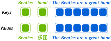
Figure 1: An example of the integration of vectorized lexical constraints into attention proposed in this work. We omit queries for simplicity. Blue and green squares denote the continuous representation of the source sentence and the constraints, respectively. The provided constraints are "Beatles$\rightarrow$Beatles" and "band$\rightarrow$乐团".

To make NMT models better learn from and cope with lexical constraints, we propose to leverage attention modules Bahdanau et al. (2015) to explicitly integrate vectorized lexical constraints. As illustrated in Figure 1, we use vectorized source constraints as additional keys and vectorized target constraints as additional values. Intuitively, the additional keys are used to estimate the relevance between the current query and the source phrases while the additional values are used to integrate the information of the target phrases. In this way, each revised attention is aware of the guidance to translate which source phrase into what target phrase.

Experiments show that our method can significantly improve the ability of NMT models to translate with constraints, indicating that the correspondence between attention keys and values is suitable for modeling constraint pairs. Inspired by recent progress in controlled text generation Dathathri et al. (2020); Pascual et al. (2021), we also introduce a plug-in to the output layer that can further improve the success rate of generating constrained tokens. We conduct experiments on four language pairs and find that our model can consistently outperform several representative baselines.

2 Neural Machine Translation

Training

The goal of machine translation is to translate a source-language sentence $\mathbf{x}=x_{1}\dots x_{|\mathbf{x}|}$ into a target-language sentence $\mathbf{y}=y_{1}\dots y_{|\mathbf{y}|}$. We use $P(\mathbf{y}|\mathbf{x};\bm{\theta})$ to denote an NMT model Vaswani et al. (2017) parameterized by $\bm{\theta}$. Modern NMT models are usually trained by maximum likelihood estimation Bahdanau et al. (2015); Vaswani et al. (2017), where the log-likelihood is defined as

$$\log P(\mathbf{y}|\mathbf{x};\bm{\theta})=\sum_{t=1}^{|\mathbf{y}|}\log P(y_{t}|\mathbf{y}_{<t},\mathbf{x};\bm{\theta}),$$ (1)

in which $\mathbf{y}_{<t}$ is a partial translation.

Inference

The inference of NMT models can be divided into two sub-processes:

• probability estimation: the model estimates the token-level probability distribution for each partial hypothesis within the beam;

• candidate selection: the decoding algorithm selects some candidates based on the probability estimated by the NMT model.

These two sub-processes are performed alternatively until reaching the maximum length or generating the end-of-sentence token.

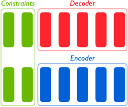
(a) Overview

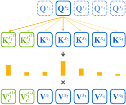
(b) Integration into enc. self-attn.

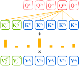
(c) Integration into dec. cross-attn.

Figure 2: Illustration of the integration of vectorized lexical constraints into both the encoder and the decoder. Blue, red, and green squares represent vectorized representations for source tokens, target tokens, and tokens of constraint pairs, respectively. The basic idea is to use source constraints as indicators to select the corresponding target constraints for each query. We only plot the attention weights for one query for simplicity.

3 Approach

This section explains how we integrate lexical constraints into NMT models. Section 3.1 illustrates the way we encode discrete constraints into continuous vectors, Section 3.2 details how we integrate the vectorized constraints into NMT models, and Section 3.3 describes our training strategy.

3.1 Vectorizing Lexical Constraints

Let $\mathbf{s}=\mathbf{s}^{(1)},\dots,\mathbf{s}^{(N)}$ be the source constraints and $\mathbf{t}=\mathbf{t}^{(1)},\dots,\mathbf{t}^{(N)}$ be the target constraints. Given a constraint pair $\langle\mathbf{s}^{(n)},\mathbf{t}^{(n)}\rangle$, lexically constrained translation requires that the system must translate the source phrase $\mathbf{s}^{(n)}$ into the target phrase $\mathbf{t}^{(n)}$. Since the inner states of NMT models are all continuous vectors rather than discrete tokens, we need to vectorize the constraints before integrating them into NMT models.

For the $n$-th constraint pair $\langle\mathbf{s}^{(n)},\mathbf{t}^{(n)}\rangle$, let $|\mathbf{s}^{(n)}|$ and $|\mathbf{t}^{(n)}|$ be the lengths of $\mathbf{s}^{(n)}$ and $\mathbf{t}^{(n)}$, respectively. We use $\mathbf{S}^{(n)}_{k}\in\mathbb{R}^{d\times 1}$ to denote the vector representation of the $k$-th token in $\mathbf{s}^{(n)}$, which is the sum of word embedding and positional embedding Vaswani et al. (2017). Therefore, the matrix representation of $\mathbf{s}^{(n)}$ is given by:

$$\mathbf{S}^{(n)}=\left[\mathbf{S}^{(n)}_{1};\dots;\mathbf{S}^{(n)}_{|\mathbf{s}^{(n)}|}\right],$$ (2)

where $\mathbf{S}^{(n)}\in\mathbb{R}^{d\times|\mathbf{s}^{(n)}|}$ is the concatenation of all vector representations of tokens in $\mathbf{s}^{(n)}$. Similarly, the matrix representation of the target constraint $\mathbf{t}^{(n)}$ is $\mathbf{T}^{(n)}\in\mathbb{R}^{d\times|\mathbf{t}^{(n)}|}$. Note that the positional embedding for each constraint is calculated independently, which is also independent of the positional embeddings of the source sentence $\mathbf{x}$ and the target sentence $\mathbf{y}$.

3.2 Integrating Vectorized Constraints

We adopt Transformer Vaswani et al. (2017) as our NMT model, which is nowadays one of the most popular and effective NMT models Liu et al. (2020). Typically, a Transformer consists of an encoder, a decoder, and an output layer, of which the encoder and decoder map discrete tokens into vectorized representations and the output layer converts such representations into token-level probability distributions. We propose to utilize the attention modules to integrate the constraints into the encoder and decoder and use a plug-in module to integrate constraints into the output layer. We change the formal representation of our model from $P(\mathbf{y}|\mathbf{x};\bm{\theta})$ to $P(\mathbf{y}|\mathbf{x},\mathbf{s},\mathbf{t};\bm{\theta})$ to indicate that the model explicitly considers lexical constraints when estimating probability.

Constraint-Related Keys and Values

We propose to map source and target constraints into additional keys and values, which are called constraint-related keys and values, in order to distinguish from the original keys and values in vanilla attention modules. In practice, source and target constraints may have different lengths and they are usually not monotonically aligned Du et al. (2021), making it challenging to directly convert the constraints into keys and values. To fix this problem, We adopt a multi-head attention layer Vaswani et al. (2017) to align the bilingual constraints. The constraint-related keys and values for the $n$-th constraint pair are given by

$$\begin{split}\mathbf{K}_{c}^{(n)}&=\mathbf{S}^{(n)},\\ \mathbf{V}_{c}^{(n)}&=\mathrm{attn}\left(\mathbf{S}^{(n)},\mathbf{T}^{(n)},\mathbf{T}^{(n)}\right),\end{split}$$ (3)

where $\mathbf{K}_{c}^{(n)}\in\mathbb{R}^{d\times|\mathbf{s}^{(n)}|}$ and $\mathbf{V}_{c}^{(n)}\in\mathbb{R}^{d\times|\mathbf{s}^{(n)}|}$. $\mathrm{attn}(\mathbf{Q},\mathbf{K},\mathbf{V})$ denotes the multi-head attention function. Note that the resulting $\mathbf{K}_{c}^{(n)}$ and $\mathbf{V}_{c}^{(n)}$ are of the same shape. $\mathbf{V}_{c}^{(n)}$ can be seen as a re-distributed version of the representation of target constraints. The constraint-related keys and values of each constraint pair are calculated separately and then concatenated together:

$$\begin{split}\mathbf{K}_{c}&=[\mathbf{K}_{c}^{(1)};\dots;\mathbf{K}_{c}^{(N)}],\\ \mathbf{V}_{c}&=[\mathbf{V}_{c}^{(1)};\dots;\mathbf{V}_{c}^{(N)}],\end{split}$$ (4)

where $\mathbf{K}_{c}\in\mathbb{R}^{d\times|\mathbf{s}|}$ and $\mathbf{V}_{c}\in\mathbb{R}^{d\times|\mathbf{s}|}$. $|\mathbf{s}|$ is the total length of all the $N$ source constraints.

Integration into the Encoder

The encoder of Transformer is a stack of $I$ identical layers, each layer contains a self-attention module to learn context-aware representations. For the $i$-th layer, the self-attention module can be represented as

$$\mathrm{attn}\left(\mathbf{H}^{(i-1)}_{\mathrm{enc}},\mathbf{H}^{(i-1)}_{\mathrm{enc}},\mathbf{H}^{(i-1)}_{\mathrm{enc}}\right),$$ (5)

where $\mathbf{H}^{(i-1)}_{\mathrm{enc}}\in\mathbb{R}^{d\times|\mathbf{x}|}$ is the output of the $(i-1)$-th layer, and $\mathbf{H}^{(0)}_{\mathrm{enc}}$ is initialized as the sum of word embedding and positional embedding Vaswani et al. (2017). For different layers, $\mathbf{H}^{(i-1)}_{\mathrm{enc}}$ may lay in various manifolds, containing different levels of information Voita et al. (2019). Therefore, we should adapt the constraint-related keys and values for each layer before the integration. We use a two-layer adaptation network to do this:

$$\begin{split}\mathbf{K}_{\mathrm{c4enc}}^{(i)}&=[\mathrm{adapt}(\mathbf{K}_{c});\mathbf{H}^{(i-1)}_{\mathrm{enc}}],\\ \mathbf{V}_{\mathrm{c4enc}}^{(i)}&=[\mathrm{adapt}(\mathbf{V}_{c});\mathbf{H}^{(i-1)}_{\mathrm{enc}}],\\ \end{split}$$ (6)

where $\mathrm{adapt}(\cdot)$ denotes the adaptation network, which consists of two linear transformations with shape $d\times d$ and a ReLU activation in between. The adaptation networks across all layers are independent of each other. $\mathbf{K}_{\mathrm{c4enc}}^{(i)}\in\mathbb{R}^{d\times(|\mathbf{s}|+|\mathbf{x}|)}$ and $\mathbf{V}_{\mathrm{c4enc}}^{(i)}\in\mathbb{R}^{d\times(|\mathbf{s}|+|\mathbf{x}|)}$ are the constraint-aware keys and values for the $i$-th encoder layer, respectively. The vanilla self-attention module illustrated in Eq. (5) is revised into the following form:

$$\mathrm{attn}\left(\mathbf{H}^{(i-1)}_{\mathrm{enc}},\mathbf{K}_{\mathrm{c4enc}}^{(i)},\mathbf{V}_{\mathrm{c4enc}}^{(i)}\right).$$ (7)

Figure 2b plots an example of the integration into the encoder self-attention.

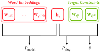
Figure 3: Illustration of the integration into the output layer. Please refer to Eq (11), (12), and (13) for the definition of $P_{\mathrm{model}}$, $P_{\mathrm{plug}}$, and $g$, respectively.

Integration into the Decoder

The integration into the decoder is similar to that into the encoder, the major difference is that we use the cross-attention module to model constraints for the decoder. The decoder of the Transformer is a stack of $J$ identical layers, each of which is composed of a self-attention, a cross-attention, and a feed-forward module. We integrate vectorized constraints into the cross-attention module for the decoder. Formally, the vanilla cross-attention is given by

$$\mathrm{attn}\left(\mathbf{S}^{(j)}_{\mathrm{dec}},\mathbf{H}^{(I)}_{\mathrm{enc}},\mathbf{H}^{(I)}_{\mathrm{enc}}\right),$$ (8)

where $\mathbf{S}^{(j)}_{\mathrm{dec}}\in\mathbb{R}^{d\times|\mathbf{y}|}$ is the output of the self-attention module in the $j$-th decoder layer, and $\mathbf{H}^{(I)}_{\mathrm{enc}}\in\mathbb{R}^{d\times|\mathbf{x}|}$ is the output of the last encoder layer. We adapt the constraint-related keys and values to match the manifold in the $j$-th decoder layer:

$$\begin{split}&\mathbf{K}_{\mathrm{c4dec}}^{(j)}=[\mathrm{adapt}(\mathbf{K}_{c});\mathbf{H}^{(I)}_{\mathrm{enc}}],\\ &\mathbf{V}_{\mathrm{c4dec}}^{(j)}=[\mathrm{adapt}(\mathbf{V}_{c});\mathbf{H}^{(I)}_{\mathrm{enc}}].\\ \end{split}$$ (9)

Then we revise the vanilla cross-attention (Eq. (8)) into the following form:

$$\mathrm{attn}\left(\mathbf{S}^{(j)}_{\mathrm{dec}},\mathbf{K}_{\mathrm{c4dec}}^{(j)},\mathbf{V}_{\mathrm{c4dec}}^{(j)}\right).$$ (10)

Figure 2c plots an example of the integration into the decoder cross-attention.

Integration into the Output Layer

In vanilla Transformer, an output layer is employed to convert the output of the last decoder layer into token-level probabilities. Let $\mathbf{h}_{t}\in\mathbb{R}^{d\times 1}$ be the decoder output at the $t$-th time step, the output probability of the Transformer model is defined as

$$P_{\mathrm{model}}(y|\mathbf{y}_{<t},\mathbf{x},\mathbf{s},\mathbf{t};\bm{\theta})=\mathrm{softmax}\left(\mathbf{h}_{t}^{\top}\mathbf{W}\right),$$ (11)

where $\mathbf{W}\in\mathbb{R}^{d\times|\mathcal{V}|}$ is the output embedding matrix and $|\mathcal{V}|$ is the vocabulary size. Inspired by the plug-and-play method Pascual et al. (2021) in the field of controlled text generation Dathathri et al. (2020); Pascual et al. (2021), we introduce an additional probability distribution over the vocabulary to better generate constrained tokens:

$$\begin{split}&P_{\mathrm{plug}}(y|\mathbf{y}_{<t},\mathbf{x},\mathbf{s},\mathbf{t};\bm{\theta})\\ &\leavevmode\nobreak\ \leavevmode\nobreak\ =\left\{\begin{split}0\quad\quad\quad\quad\quad\quad\quad\quad\quad\quad\quad&\quad y\notin\mathbf{t}\\ \mathrm{max}\left(0,\mathrm{cos}\left(\frac{\mathbf{w}_{y}}{|\mathbf{w}_{y}|},\frac{\mathbf{h}_{t}}{|\mathbf{h}_{t}|}\right)\right)&\quad y\in\mathbf{t}\\ \end{split}\right.\end{split},$$ (12)

where $\mathbf{w}_{y}\in\mathbf{R}^{d\times 1}$ is the word embedding of token $y$ and $\mathbf{t}$ is the sequence of all the target-side constrained tokens. We also use a gating sub-layer to control the strength of the additional probability:

$$\begin{split}&g(y,\mathbf{h}_{t})\\ &\leavevmode\nobreak\ \leavevmode\nobreak\ =\mathrm{sigmoid}\left(\mathrm{tanh}\left(\left[\mathbf{w}_{y}^{\top}\mathbf{W}_{1};\mathbf{h}_{t}^{\top}\mathbf{W}_{2}\right]\right)\mathbf{W}_{3}\right),\end{split}$$ (13)

where $\mathbf{W}_{1}\in\mathbf{R}^{d\times d}$, $\mathbf{W}_{2}\in\mathbf{R}^{d\times d}$, and $\mathbf{W}_{3}\in\mathbf{R}^{2d\times 1}$ are three trainable linear transformations. The final output probability is given by

$$\begin{split}&P(y|\mathbf{y}_{<t},\mathbf{x},\mathbf{s},\mathbf{t};\bm{\theta})\\ &\leavevmode\nobreak\ \leavevmode\nobreak\ =\left(1-g(y,\mathbf{h}_{t})\right)P_{\mathrm{model}}(y|\mathbf{y}_{<t},\mathbf{x},\mathbf{s},\mathbf{t};\bm{\theta})\\ &\leavevmode\nobreak\ \leavevmode\nobreak\ +g(y,\mathbf{h}_{t})P_{\mathrm{plug}}(y|\mathbf{y}_{<t},\mathbf{x},\mathbf{s},\mathbf{t};\bm{\theta}).\end{split}$$ (14)

3.3 Training and Inference

Training

The proposed constraint-aware NMT model should not only generate pre-specified constraints but also maintain or improve the translation quality compared with vanilla NMT models. We thus propose to distinguish between constraint tokens and constraint-unrelated tokens during training. Formally, the training objective is given by

$$\begin{split}&L(\mathbf{y}|\mathbf{x},\mathbf{s},\mathbf{t};\bm{\theta})\\ &\leavevmode\nobreak\ \leavevmode\nobreak\ =\alpha\sum_{y_{t}\in\mathbf{y}\cap\mathbf{t}}\log P(y_{t}|\mathbf{y}_{<t},\mathbf{x},\mathbf{s},\mathbf{t};\bm{\theta})\\ &\leavevmode\nobreak\ \leavevmode\nobreak\ +\leavevmode\nobreak\ \beta\sum_{y_{t}\in\mathbf{y}\setminus\mathbf{t}}\log P(y_{t}|\mathbf{y}_{<t},\mathbf{x},\mathbf{s},\mathbf{t};\bm{\theta}),\end{split}$$ (15)

where $\alpha$ and $\beta$ are hyperparameters to balance the learning of constraint generation and translation.

We can divide the parameter set of the whole model into two subsets: $\bm{\theta}=\bm{\theta}_{v}\cup\bm{\theta}_{c}$, where $\bm{\theta}_{v}$ is a set of original vanilla model parameters and $\bm{\theta}_{c}$ is a set of newly-introduced parameters that are used to vectorize and integrate lexical constraints. Since $\bm{\theta}_{c}$ is significantly smaller than $\bm{\theta}_{v}$, it requires much less training iterations. Therefore, we adopt the strategy of two-stage training Tu et al. (2018); Zhang et al. (2018) for model optimization. Specifically, we optimize $\bm{\theta}_{v}$ using the standard NMT training objective Bahdanau et al. (2015); Vaswani et al. (2017) at the first stage and then learn the whole model $\bm{\theta}$ at the second stage. The second stage is significantly shorter than the first stage, we will give more details in Section 4.1.

Inference

As discussed in Section 2, the inference process is composed of two sub-processes: probability estimation and candidate selection. In this work, we aim to improve the probability estimation sub-process and our method is orthogonal to constrained decoding algorithms Hokamp and Liu (2017); Post and Vilar (2018); Hu et al. (2019), which instead focus on candidate selection. Therefore, we can employ not only beam search but also constrained decoding algorithms at inference time. We use VDBA Hu et al. (2019) as the default constrained decoding algorithm, which supports batched inputs and is significantly faster than most other counterparts Hokamp and Liu (2017); Post and Vilar (2018); Hasler et al. (2018).

4 Experiments

4.1 Setup

Training Data

In this work, we conduct experiments on Chinese$\Leftrightarrow$English (Zh$\Leftrightarrow$En) and German$\Leftrightarrow$English (De$\Leftrightarrow$En) translation tasks. For Zh$\Leftrightarrow$En, the training set contains 1.25M sentence pairs from LDC. For De$\Leftrightarrow$En, the training set is from the WMT 2014 German$\Leftrightarrow$English translation task, which consists of 4.47M sentence pairs. We apply BPE Sennrich et al. (2016b) with 32K joint merge operations for both Zh$\Leftrightarrow$En and De$\Leftrightarrow$En.

Evaluation Data

Following Chen et al. (2021b), we evaluate our approach on the test sets with human-annotated alignments, which are widely used in related studies Chen et al. (2020b, 2021a). We find the alignment test sets have significant overlaps with the corresponding training sets, which is not explicitly stated in previous works. In this work, we remove the training examples that are covered by the alignment test sets. For Zh$\Leftrightarrow$En, we use the alignment datasets from Liu et al. (2005), in which the validation and test sets both contain 450 sentence pairs. For De$\Leftrightarrow$En, we use the alignment dataset from Zenkel et al. (2020) as the test set, which consists of 508 sentence pairs. Since there is no human-annotated alignment validation sets for De$\Leftrightarrow$En, we use fast-align to annotate the newstest 2013 as the validation set for De$\Leftrightarrow$En.

Lexical Constraints

In real-world applications, lexical constraints are usually provided by human translators. We follow Chen et al. (2021b) to simulate the practical scenario by sampling constraints from the phrase pairs that are extracted from parallel data using alignments. The script for phrase pair extraction is publicly available. For the validation and test sets of Zh$\Leftrightarrow$En and the test set of De$\Leftrightarrow$En, we use human-annotated alignments to extract phrase pairs. For the training corpora in both Zh$\Leftrightarrow$En and De$\Leftrightarrow$En, we use fast-align to firstly learn an alignment model and then use the model to automatically annotate the alignments. The validation set of De$\Leftrightarrow$En is also annotated by the alignment model learned on the corresponding training corpus. We use the same strategy as Chen et al. (2021b) to sample constraints from the extracted phrase pairs. More concretely, the number of constraints in each sentence is up to 3. The length of each constrained phrase is uniformly sampled among 1 and 3. For each sentence pair, all the constraint pairs are shuffled and then supplied to the model in an unordered manner.

Method	BLEU					CSR (%)
	Z$\rightarrow$E	E$\rightarrow$Z	D$\rightarrow$E	E$\rightarrow$D	Avg.	Z$\rightarrow$E	E$\rightarrow$Z	D$\rightarrow$E	E$\rightarrow$D	Avg.
Vanilla	30.4	56.1	31.7	24.5	35.7	26.9	30.5	19.2	13.8	22.6
VDBA	31.6	56.4	35.0	27.9	37.7	99.4	98.9	100.0	100.0	99.6
Replace	33.6	58.3	34.9	28.1	38.7	89.7	90.2	93.2	90.7	91.0
CDAlign	32.1	58.0	35.2	28.3⋆	38.4	87.4	90.0	96.8	95.7	92.5
Ours	34.4	59.1	35.9	28.8	39.6	99.4	98.9	100.0	100.0	99.6

Table 1: Results on lexically constrained test sets. "Z$\rightarrow$E" denotes Zh$\rightarrow$En, and "D$\rightarrow$E" denotes De$\rightarrow$En. The best BLEU in each column is highlighted in bold, and "$\star$" indicates no significant difference with the method achieving the best BLEU. The best CSR in each column is italicized.

Model Configuration

We use the base setting Vaswani et al. (2017) for our model. Specifically, the hidden size $d$ is 512 and the depths of both the encoder and the decoder are 6. Each multi-head attention module has 8 individual attention heads. Since our method introduces additional parameters, we use a larger model with an 8-layer encoder and an 8-layer decoder to assimilate the parameter count for the baselines. For Zh$\Leftrightarrow$En, we optimize $\bm{\theta}_{v}$ for 50K iterations at the first stage and then optimize $\bm{\theta}$ for 10K iterations at the second stage. For a fair comparison, we train the baselines for 60K iterations in total. For De$\Leftrightarrow$En, we optimize $\bm{\theta}_{v}$ for 90K iterations then optimize $\bm{\theta}$ for 10K iterations. The baselines are trained for 100K iterations. All the involved models are optimized by Adam Kingma and Ba (2015), with $\beta_{1}=0.9$, $\beta_{2}=0.98$ and $\epsilon=10^{-9}$. The dropout rate is set to 0.3 for Zh$\Leftrightarrow$En and 0.1 for De$\Leftrightarrow$En. Label smoothing is employed and the smoothing penalty is set to 0.1 for all language pairs. We use the same learning rate schedule as Vaswani et al. (2017). All models are trained on 4 NVIDIA V100 GPUs and evaluated on 1 NVIDIA V100 GPU. During training, each mini batch contains roughly 32K tokens in total across all GPUs. We set the values of $\alpha$ and $\beta$ based on the results on the validation set. Specifically, for models using VDBA, we set $\alpha=\beta=0.5$, while for models using beam search, we set $\alpha=0.8$ and $\beta=0.2$. The beam size is set to $4$ during inference.

Baselines

We compare our approach with three representative baselines:

• VDBA Hu et al. (2019): dynamically devoting part of the beam for constraint-related hypotheses at inference time;

• Replace Song et al. (2019): directly replacing source constraints in the training data with their corresponding target constraints. The model is also improved with pointer network;

• CDAlign Chen et al. (2021b): explicitly using an alignment model to decide the position to insert target constraints during inference.

Evaluation Metrics

We evaluate the involved methods using the following two metrics:

• BLEU: we use sacreBLEU Post (2018) to report the BLEU score;

• Copying Success Rate (CSR): We follow Chen et al. (2021b) to use the percentage of constraints that are successfully generated in the translation as the CSR, which is calculated at word level after removing the BPE separator.

We use compare-mt Neubig et al. (2019) for significance testing, with $\mathrm{bootstrap}=1000$ and $\mathrm{prob\_thresh}=0.05$.

4.2 Main Results

Table 1 shows the results of lexically constrained translation on test sets of all four translation tasks. All the investigated methods can effectively improve the CSR over the vanilla Transformer. The CSR of VDBA on Zh$\Leftrightarrow$En is not 100.0% for the reason that some target constraints contain out-of-vocabulary tokens. Replace Song et al. (2019) achieves better BLEU scores on three translation directions (i.e., Zh$\Leftrightarrow$En and En$\rightarrow$De) than VDBA, but its CSR is much lower. CDAlign Chen et al. (2021b) also performs better than Replace on average regarding CSR. Our method consistently outperforms all the three baselines across the four translation directions in terms of BLEU, demonstrating the necessity of integrating vectorized constraints into NMT models. Decoding with VDBA, we also achieve the highest CSR. To disentangle the effect of integrating vectorized constraints and VDBA, we also report the result of our model using beam search in Table 2. Decoding with beam search, our model can also achieve a better BLEU score than the baselines and the CSR is higher than both Replace and CDAlign on average.

Metric	Z$\rightarrow$E	E$\rightarrow$Z	D$\rightarrow$E	E$\rightarrow$D	Avg.
BLEU	34.5	59.5	35.7	28.6	39.6
CSR (%)	94.6	92.4	97.3	93.3	94.4

Table 2: Performance on lexically constrained test sets of the proposed model decoding with beam search.

Integration		DA	BLEU	CSR (%)
Attention	Output
✓	×	B	34.3	91.5
×	✓		32.6	61.9
✓	✓		34.5	94.2
✓	×	V	34.4	98.6
×	✓		33.5	98.6
✓	✓		34.7	98.6

Table 3: Effect of different components. The results are reported on the Zh$\rightarrow$En validation set. "Attention": the constraint integration of attention modules. "Output": the integration into the output layer. "DA": decoding algorithm. "B": beam search. "V": VDBA.

4.3 Ablation Study

We investigate the effect of different components through an ablation study, the results are shown in Table 3. We find that only integrating lexical constraints into attention can significantly improve the CSR over the vanilla model (91.5% vs. 25.5%), which is consistent with our motivation that the correspondence between keys and values is naturally suitable for modeling the relation between source and target constraints. Plugging target constraints into the output layer can further improve the performance, but the output plug-in itself can only generate 61.9% of constraints. When decoding with VDBA, combining both the two types of integration achieves the best BLEU score, indicating that every component is important for the model to translate with constraints.

Method	BLEU
	Z$\rightarrow$E	E$\rightarrow$Z	D$\rightarrow$E	E$\rightarrow$D
Vanilla	29.7	52.9	29.3	23.5
VDBA	31.4	54.0	31.8	26.2
Replace	31.8	56.0	31.1	25.7
CDAlign	32.3	55.1	32.2	26.4
Ours	33.1⋆	56.5⋆	32.7⋆	27.0⋆
w/o VDBA	33.5	56.7	32.9	27.1

(a) BLEU score on code-switched test sets.

Method	CSR (%)
	Z$\rightarrow$E	E$\rightarrow$Z	D$\rightarrow$E	E$\rightarrow$D
Vanilla	12.7	14.4	10.2	8.7
VDBA	99.4	98.5	100.0	100.0
Replace	44.8	47.4	44.9	44.1
CDAlign	89.3	89.5	95.2	91.1
Ours	99.4	98.5	100.0	100.0
w/o VDBA	96.1	94.6	97.6	95.8

(b) CSR on code-switched test sets.

Table 4: Results on the code-switched translation task.

4.4 Code-Switched Translation

Task Description and Data Preparation

An interesting application of lexically constrained machine translation is code-switched translation, of which the output contains terms across different languages. Figure 1 shows an example of code-switched translation, where the output Chinese sentence should include the English token "Beatles". Code-switched machine translation is important in many scenarios, such as entity translation Li et al. (2018) and the translation of sentences containing product prices or web URLs Chen et al. (2021b). In this work, we evaluate the performance of several approaches on code-switched machine translation. The parallel data and extracted constraint pairs for each language pair are the same as those used in the lexically constrained translation task. To construct the training and evaluation data for code-switched translation, we randomly replace 50% of the target constraints with their corresponding source constraints. The target sentence is also switched if it contains switched target constraints.

Results

Table 4 gives the results of the code-switched translation task. The CSR of Replace Song et al. (2019) is lower than 50% across all the four translation directions, indicating that simply replacing the training data can not handle the code-switched translation. A potential reason is that it is difficult for the NMT model to decide whether to translate or copy some source phrases in the input sentence. Surprisingly, VDBA, CDAlign, and our method all perform well in this scenario, and our method outperforms the two baselines. These results suggest the capability of our method to cope with flexible types of lexical constraints.

5 Discussion

Method	Batch Size (# Sent.)
	1	128
Vanilla	1.0×	43.2×
VDBA	0.5×	2.1×
Replace	0.9×	40.5×
CDAlign	0.7×	n/a
Ours	0.5×	2.3×
w/o VDBA	0.9×	39.2×

Table 5: Inference speed with different batch sizes.

5.1 Inference Speed

We report the inference speed of each involved approach in Table 5. The speed of Replace is close to that of the vanilla Transformer, but its CSR is much lower than other methods. Since the open-sourced implementation of CDAlign does not support batched decoding, we compare our method with CDAlign with $\mathrm{batch\_size}=1$. The speed of our method using beam search is faster than that of CDAlign (0.9×vs. 0.7×). When provided with batched inputs, our method can slightly speed up VDBA (2.3×vs. 2.1×). A potential reason is that the probability estimated by our model is more closely related to the correctness of the candidates, making target constraints easier to find.

Model	DA	Prob.		ECE(↓)
		All	Const.
Vanilla	B	0.69	0.74	8.03
Ours		0.70	0.80	7.19
Vanilla	V	0.64	0.42	10.73
Ours		0.67	0.61	7.72

Table 6: Inference ECE on the Zh$\rightarrow$En validation set. "All": the average probability of all predicted tokens. "Const.": the average probability of constrained tokens.

5.2 Calibration

To validate whether the probability of our model is more accurate than vanilla models, we follow Wang et al. (2020) to investigate the gap between the probability and the correctness of model outputs, which is measured by the inference expected calibration error (ECE). As shown in Table 6, the inference ECE of our method is much lower than that of the vanilla model, indicating that the probability of our model is more accurate than vanilla models. To better understand the calibration of our model and the baseline model, we also estimate the average probability of all the predicted tokens and the constrained tokens. The results show that our model assigns higher probabilities to constrained tokens, which are already known to be correct.

5.3 Memory vs. Extrapolation

Z$\rightarrow$E	E$\rightarrow$Z	D$\rightarrow$E	E$\rightarrow$D	Avg.
38.9%	43.4%	27.7%	32.2%	35.6%

Table 7: Overlap ratio of lexical constraints between training and test sets across the four directions.

To address the concern that the proposed model may only memorize the constraints seen in the training set, we calculate the overlap ratio of constraints between training and test sets. As shown in Table 7, we find that only 35.6% of the test constraints are seen in the training data, while the CSR of our model decoding with beam search is 94.4%. The results indicate that our method extrapolates well to constraints unseen during training.

5.4 Case Study

Table 8 shows some example translations of different methods. We find Replace tends to omit some constraints. Although VDBA and CDAlign can successfully generate constrained tokens, the translation quality of the two methods is not satisfying. Our result not only contains constrained tokens but also maintains the translation quality compared with the unconstrained model, confirming the necessity of integrating vectorized constraints into NMT models.

Constraints	Zielsetzung $\rightarrow$ objectives, Fiorella $\rightarrow$ Fiorella
Source	Mit der Zielsetzung des Berichtes von Fiorella Ghilardotti allerdings sind wir einverstanden .
Reference	Even so , we do agree with the objectives of Fiorella Ghilardotti’s report .
Vanilla	However , we agree with the aims of the Ghilardotti report .
VDBA	Fiorella’s Ghilardotti report , however , has our objectives of being one which we agree with .
Replace	However , we agree with the objectives of the Ghilardotti report .
CDAlign	However , we agree with objectives of Fi Fiorella Ghilardotti’s report .
Ours	We agree with the objectives of Fiorella Ghilardotti’s report , however .

Table 8: Example translations of different lexically constrained NMT approaches.

6 Related Work

6.1 Lexically Constrained NMT

One line of approaches to lexically constrained NMT focuses on designing advanced decoding algorithms Hasler et al. (2018). Hokamp and Liu (2017) propose grid beam search (GBS), which enforces target constraints to appear in the output by enumerating constraints at each decoding step. The beam size required by GBS varies with the number of constraints. Post and Vilar (2018) propose dynamic beam allocation (DBA) to fix the problem of varying beam size for GBS, which is then extended by Hu et al. (2019) into VDBA that supports batched decoding. There are also some other constrained decoding algorithms that leverage word alignments to impose constraints Song et al. (2020); Chen et al. (2021b). Although the alignment-based decoding methods are faster than VDBA, they may be negatively affected by noisy alignments, resulting in low CSR. Recently, Susanto et al. (2020) adopt Levenshtein Transformer Gu et al. (2019) to insert target constraints in a non-autoregressive manner, for which the constraints must be provided with the same order as that in the reference.

Another branch of studies proposes to edit the training data to induce constraints Sennrich et al. (2016a). Song et al. (2019) directly replace source constraints with their target translations and Dinu et al. (2019) insert target constraints into the source sentence without removing source constraints. Similarly, Chen et al. (2020a) propose to append target constraints after the source sentence.

In this work, we propose to integrate vectorized lexical constraints into NMT models. Our work is orthogonal to both constrained decoding and constraint-oriented data augmentation. A similar work to us is that Li et al. (2020) propose to use continuous memory to store only the target constraint, which is then integrated into NMT models through the decoder self-attention. However, Li et al. (2020) did not exploit the correspondence between keys and values to model both source and target constraints.

6.2 Controlled Text Generation

Recent years have witnessed rapid progress in controlled text generation. Dathathri et al. (2020) propose to use the gradients of a discriminator to control a pre-trained language model to generate towards a specific topic. Liu et al. (2021) propose a decoding-time method that employs experts to control the generation of pre-trained language models.

We borrow the idea presented in Pascual et al. (2021) to insert a plug-in into the output layer. The difference between our plug-in network and Pascual et al. (2021) is that we use an input-dependent gate to control the effect of the plugged probability.

7 Conclusion

In this work, we propose to vectorize and integrate lexical constraints into NMT models. Our basic idea is to use the correspondence between keys and values in attention modules to model constraint pairs. Experiments show that our approach can outperform several representative baselines across four different translation directions. In the future, we plan to vectorize other attributes, such as the topic, the style, and the sentiment, to better control the generation of NMT models.

References

- Bahdanau et al. (2015) Dzmitry Bahdanau, Kyunghyun Cho, and Yoshua Bengio. 2015. Neural machine translation by jointly learning to align and translate. In ICLR.
- Chen et al. (2021a) Chi Chen, Maosong Sun, and Yang Liu. 2021a. Mask-align: Self-supervised neural word alignment. In ACL.
- Chen et al. (2021b) Guanhua Chen, Yun Chen, and Victor O.K. Li. 2021b. Lexically constrained neural machine translation with explicit alignment guidance. In AAAI, pages 12630–12638.
- Chen et al. (2020a) Guanhua Chen, Yun Chen, Yong Wang, and Victor O.K. Li. 2020a. Lexical-constraint-aware neural machine translation via data augmentation. In IJCAI.
- Chen et al. (2020b) Yun Chen, Yang Liu, Guanhua Chen, Xin Jiang, and Qun Liu. 2020b. Accurate word alignment induction from neural machine translation. In EMNLP.
- Dathathri et al. (2020) Sumanth Dathathri, Andrea Madotto, Janice Lan, Jane Hung, Eric Frank, Piero Molino, Jason Yosinski, and Rosanne Liu. 2020. Plug and play language models: A simple approach to controlled text generation. In ICLR.
- Dinu et al. (2019) Georgiana Dinu, Prashant Mathur, Marcello Federico, and Yaser Al-Onaizan. 2019. Training neural machine translation to apply terminology constraints. In ACL.
- Du et al. (2021) Cunxiao Du, Zhaopeng Tu, and Jing Jiang. 2021. Order-agnostic cross entropy for non-autoregressive machine translation. In ICML.
- Gu et al. (2019) Jiatao Gu, Changhan Wang, and Junbo Zhao. 2019. Levenshtein transformer. In NeurIPS.
- Hasler et al. (2018) Eva Hasler, Adrià de Gispert, Gonzalo Iglesias, and Bill Byrne. 2018. Neural machine translation decoding with terminology constraints. In NAACL.
- Hokamp and Liu (2017) Chris Hokamp and Qun Liu. 2017. Lexically constrained decoding for sequence generation using grid beam search. In ACL.
- Hu et al. (2019) J. Edward Hu, Huda Khayrallah, Ryan Culkin, Patrick Xia, Tongfei Chen, Matt Post, and Benjamin Van Durme. 2019. Improved lexically constrained decoding for translation and monolingual rewriting. In NAACL.
- Kingma and Ba (2015) Diederik P. Kingma and Jimmy Ba. 2015. Adam: A method for stochastic optimization. CoRR, abs/1412.6980.
- Koehn (2009) Philipp Koehn. 2009. A process study of computer-aided translation. Machine Translation, 23(4):241–263.
- Koehn et al. (2007) Philipp Koehn, Hieu Hoang, Alexandra Birch, Chris Callison-Burch, Marcello Federico, Nicola Bertoldi, Brooke Cowan, Wade Shen, Christine Moran, Richard Zens, Chris Dyer, Ondrej Bojar, Alexandra Constantin, and Evan Herbst. 2007. Moses: Open source toolkit for statistical machine translation. In ACL.
- Li et al. (2020) Huayang Li, Guoping Huang, Deng Cai, and Lemao Liu. 2020. Neural machine translation with noisy lexical constraints. IEEE/ACM Transactions on Audio, Speech, and Language Processing, 28:1864–1874.
- Li et al. (2018) Xiaoqing Li, Jinghui Yan, Jiajun Zhang, and Chengqing Zong. 2018. Neural name translation improves neural machine translation. In CWMT.
- Liu et al. (2021) Alisa Liu, Maarten Sap, Ximing Lu, Swabha Swayamdipta, Chandra Bhagavatula, Noah A. Smith, and Yejin Choi. 2021. DExperts: Decoding-time controlled text generation with experts and anti-experts. In ACL 2021.
- Liu et al. (2005) Yang Liu, Qun Liu, and Shouxun Lin. 2005. Log-linear models for word alignment. In ACL.
- Liu et al. (2020) Yinhan Liu, Jiatao Gu, Naman Goyal, Xian Li, Sergey Edunov, Marjan Ghazvininejad, Mike Lewis, and Luke Zettlemoyer. 2020. Multilingual denoising pre-training for neural machine translation. Transactions of the ACL, 8:726–742.
- Neubig et al. (2019) Graham Neubig, Zi-Yi Dou, Junjie Hu, Paul Michel, Danish Pruthi, and Xinyi Wang. 2019. compare-mt: A tool for holistic comparison of language generation systems. In NAACL (Demo).
- Pascual et al. (2021) Damian Pascual, Beni Egressy, Clara Meister, Ryan Cotterell, and Roger Wattenhofer. 2021. A plug-and-play method for controlled text generation.
- Post (2018) Matt Post. 2018. A call for clarity in reporting BLEU scores. In WMT.
- Post and Vilar (2018) Matt Post and David Vilar. 2018. Fast lexically constrained decoding with dynamic beam allocation for neural machine translation. In NAACL.
- Sennrich et al. (2016a) Rico Sennrich, Barry Haddow, and Alexandra Birch. 2016a. Controlling politeness in neural machine translation via side constraints. In NAACL.
- Sennrich et al. (2016b) Rico Sennrich, Barry Haddow, and Alexandra Birch. 2016b. Neural machine translation of rare words with subword units. In ACL.
- Song et al. (2020) Kai Song, Kun Wang, Heng Yu, Yue Zhang, Zhongqiang Huang, Weihua Luo, Xiangyu Duan, and Min Zhang. 2020. Alignment-enhanced transformer for constraining nmt with pre-specified translations. In AAAI.
- Song et al. (2019) Kai Song, Yue Zhang, Heng Yu, Weihua Luo, Kun Wang, and Min Zhang. 2019. Code-switching for enhancing NMT with pre-specified translation. In NAACL.
- Susanto et al. (2020) Raymond Hendy Susanto, Shamil Chollampatt, and Liling Tan. 2020. Lexically constrained neural machine translation with Levenshtein transformer. In ACL.
- Tu et al. (2018) Zhaopeng Tu, Yang Liu, Shuming Shi, and Tong Zhang. 2018. Learning to remember translation history with a continuous cache. Transactions of the Association for Computational Linguistics, 6:407–420.
- Vaswani et al. (2017) Ashish Vaswani, Noam Shazeer, Niki Parmar, Jakob Uszkoreit, Llion Jones, Aidan N Gomez, Łukasz Kaiser, and Illia Polosukhin. 2017. Attention is all you need. In NeurIPS.
- Voita et al. (2019) Elena Voita, Rico Sennrich, and Ivan Titov. 2019. The bottom-up evolution of representations in the transformer: A study with machine translation and language modeling objectives. In EMNLP.
- Wang et al. (2020) Shuo Wang, Zhaopeng Tu, Shuming Shi, and Yang Liu. 2020. On the inference calibration of neural machine translation. In ACL.
- Zenkel et al. (2020) Thomas Zenkel, Joern Wuebker, and John DeNero. 2020. End-to-end neural word alignment outperforms GIZA++. In ACL.
- Zhang et al. (2021) Jiacheng Zhang, Huanbo Luan, Maosong Sun, Feifei Zhai, Jingfang Xu, and Yang Liu. 2021. Neural machine translation with explicit phrase alignment. IEEE/ACM Transactions on Audio, Speech, and Language Processing, 29:1001–1010.
- Zhang et al. (2018) Jiacheng Zhang, Huanbo Luan, Maosong Sun, Feifei Zhai, Jingfang Xu, Min Zhang, and Yang Liu. 2018. Improving the transformer translation model with document-level context. In EMNLP.