Dynamic behavior for a gradient algorithm with energy and momentum

Abstract.

This paper investigates a novel gradient algorithm, using both energy and momentum (called AGEM), for solving general non-convex optimization problems. The solution properties of the AGEM algorithm, including uniformly boundedness and convergence to critical points, are examined. The dynamic behavior is studied through analysis of a high resolution ODE system. Such ODE system is nonlinear and obtained by taking the limit of the discrete scheme while keeping the momentum effect through a rescale of the momentum parameter. In particular, we show global well-posedness of the ODE system, time-asymptotic convergence of solution trajectories, and further establish a linear convergence rate for objective functions satisfying the Polyak-Łojasiewicz condition.

1. Introduction

In this paper we will be considering the unconstrained optimization problem,

(1.1) $$\min_{\theta\in\mathbb{R}^{n}}f(\theta),$$

where the objective function $f:\mathbb{R}^{n}\to\mathbb{R}$ is assumed to be differentiable and bounded from below, i.e., $f+c>0$ for some $c\in\mathbb{R}$. The most prominent applications such as training machine learning models have involved large-scale problems in which the objective function is typically non-convex and in the form of a finite sum over terms associated with individual data. In this setting, first-order gradient methods such as gradient descent (GD) and its variants are often applied since they are computationally efficient and has satisfying performance [11]; consequently, there has been much effort on the theory and practices of speeding up the convergence of first-order gradient methods, among which adaptive step size [36, 21] and momentum [32] are two widely-used techniques.

AEGD (adaptive gradient descent with energy) is a gradient method that was first introduced by us in [25]. The distinct feature of AEGD is the use of an additional energy variable so that the resulting algorithm is unconditionally energy stable regardless of the base learning rate. In this work, we study a variant of AEGD with momentum (termed as AGEM), which takes the following form: starting from $\theta_{0}$ and $r_{0}=F(\theta_{0})$ with $F=\sqrt{f+c}$, inductively define

(1.2a) $$v_{k} =\beta v_{k-1}+(1-\beta)\nabla F(\theta_{k}),\quad v_{-1}=\bf{0},$$

(1.2b) $$r_{k+1} =\frac{r_{k}}{1+2\eta|v_{k}|^{2}},$$

(1.2c) $$\theta_{k+1} =\theta_{k}-2\eta r_{k+1}v_{k},$$

where $\beta\in(0,1)$ is the momentum parameter. This when taking $\beta=0$ reduces to the original AEGD in [25]. AGEM (1.2) is comparable to the SGEM (Stochastic Gradient with energy and momentum) algorithms introduced in [26]. In sharp contrast to GD, all these energy-adaptive gradient methods feature the unconditional energy stability property, irrespective of the base step size $\eta$. The excellent performance of AEGD type schemes has been demonstrated with various optimization tasks [25, 26]. On the theoretical side, the existing convergence rates depend on $kr_{k}$, instead of only $k$; this could degrade the convergence behavior when the energy variable decays too fast. This issue consists of one of the main challenges to reach a better understanding of the class of energy-adaptive gradient methods.

On the other hand, the connection between ODEs and numerical optimization can be established via taking step sizes to be very small so that the trajectory or solution path converges to a curve modeled by an ODE. The well-established theory and dynamic properties of ODEs can provide deeper insights into optimization; see e.g., [2, 6, 4, 35].

In this work, we therefore derive an ODE system for (1.2), which is the exact limit of (1.2) by taking small step sizes while keeping $\epsilon=\beta\eta/(1-\beta)$ fixed. This ODE system with unknown $U:=(v,r,\theta)$ reads

(1.3a) $$\epsilon\dot{v} =-v+\nabla F(\theta),$$

(1.3b) $$\dot{r} =-2r|v|^{2},$$

(1.3c) $$\dot{\theta} =-2rv,$$

for $t>0$, with initial conditions $U(0)=(0,F(\theta_{0}),\theta_{0})$; here, $\theta_{0}$ is the starting point in the AGEM scheme, $\dot{U}$ denotes the time derivative. This work is the first to model AEGD-type schemes by ODE systems. With this connection, the convergence properties of (1.2) will be studied from the perspective of continuous dynamics for general smooth objective functions.

For a gradient method, the geometric property of $f$ often affects the convergence and convergence rates. For non-convex $f$, we consider an old condition originally introduced by Polyak [31], who showed it is a sufficient condition for GD to achieve a linear convergence rate; see [20] for a recent convergence study under this condition. Such a condition is called the Polyak-Łojasiewicz (PL) inequality in the literature since it is a special case of the gradient inequality introduced by Łojasiewicz in 1963 [27]. For optimization-related dynamical systems, it was observed for a long time that in general only convergence along subsequences can be obtained. For convergence of the whole trajectory, some more involved geometric properties are required; for instance, the Łojasiewicz inequality has been used to get convergence of trajectory in [3] for a second-order gradient-like dissipative dynamical system with Hessian-driven damping. In Section 7, we shall show such inequality can ensure the trajectory convergence for $\theta(t)$ in (1.3). We should point out that a number of important non-convex problems in machine learning, including some classes of neural networks, have been recently shown to satisfy the PL condition [7, 13, 34, 24]. It is believed that the PL/KL condition provides a relevant and attractive setting for many machine learning problems, particularly in the over-parametrized regime.

Contributions We study the convergence behavior of both the discrete scheme (1.2) and its continuous counterpart (1.3). Our main contributions are summarized as follows.

1. For (1.2), we prove that the iterates are uniformly bounded and converge to the set of critical points of the objective function when the step size is suitably small, also $\lim_{k\to\infty}r_{k}=r^{*}>0$.

2. We derive (1.3) as a high resolution ODE system of the discrete scheme (1.2). For this ODE system, we first show the global well-posedness by constructing a suitable Lyapunov function. We then establish the time-asymptotic convergence of the solution towards critical points using the Lasalle invariance principle. Moreover, a positive lower bound of the energy variable is provided.

3. For objective functions that satisfy the PL condition (see Section 2.2), we are able to establish a linear convergence rate

   $$f(\theta(t))-f(\theta^{*})\leq(f(\theta_{0})-f(\theta^{*}))e^{-\beta t}$$

   for some $\beta>0$, where $\theta^{*}$ is the global minimizer of $f$ (not necessarily convex).

4. We propose a few variations and extensions: for a larger class of objective functions satisfying the Łojasiewicz inequality, $\theta(t)$ is shown to have finite length, hence converging to a single minimum of $f$, with associated convergence rates.

For non-convex optimization problems, obtaining convergence rates is a challenging task. The technique used in Section 6 to obtain the linear convergence rate for system (1.3) is inspired by that used in [4], where a linear convergence rate was obtained for the Heavy Ball dynamical system, that is (1.4) with $a(t)$ being a constant. For the more complicated nonlinear system (1.3), we are able to construct a class of control functions which play a similar role to that in [4]. The proof of the convergence rate results for (1.3) is significantly different and more involved. In particular, we explore a subtle optimization argument to identify an optimal control function to achieve the desired decay rate.

Further related works. A recent line of research on the theoretical analysis of accelerated gradient algorithms has been on the study of their continuous-time limits (ODEs). With well-established theory and techniques such as Lyapunov functions, ODEs prove to be very useful when studying the convergence of a discrete algorithm. The convergence behavior of the heavy ball method has been studied via the following second-order ODE:

(1.4) $$\ddot{\theta}(t)+a(t)\dot{\theta}+\nabla f(\theta)=0,\quad\theta(0)=\theta_{0},\quad\dot{\theta}=0$$

with $a(t)$ being a smooth, positive and non-increasing function. The Lyapunov function $E=\frac{1}{2}|\dot{\theta}|^{2}+f(\theta)$ for (1.4) plays an essential role in analysis for both convex setting [2] and non-convex setting [6]. The Nesterov algorithm is shown to be connected to (1.4) with $a(t)=\frac{3}{t}$ in [35], where the authors recover the optimal convergence rate of $O(1/t^{2})$ of the discrete scheme in the convex setting [30]. A non-autonomous system of differential equations was derived and analyzed in [14] as the continuous time limit of adaptive optimization methods including Adam and RMSprop. In addition to convergence behavior, such dynamical approach also allows for better understanding of qualitative features of some discrete algorithms. For example, [33] investigated the difference between the acceleration phenomena of the heavy ball method and the Nesterov algorithm by analyzing some high-resolution ODEs. By analyzing the sign GD of form $\dot{\theta}=-\frac{\nabla f(\theta)}{|\nabla f(\theta)|}$ and its variants, [29] identified three behavior patterns of Adam and RMSprop: fast initial progress, small oscillations, and large spikes. From a continuous dynamical system satisfying nice converging properties, one may discretize it to obtain novel algorithms; for example, a new second-order inertial optimization method (called INNA algorithm) is obtained from a continuous inclusion system when the objective function is non-smooth [12]. To our knowledge, (1.3) is different from the priori ODEs for optimization methods, and also subtle to analyze.

The rest of the paper is organized as follows. In Section 2, we begin with the problem setup, recall the existing energy-adaptive gradient methods and propose a new method. The PL condition and related properties are discussed. In Section 3, we analyze the solution properties of the proposed method. In Section 4, we derive a continuous dynamical system and present a convergence result to show the dynamical system is a faithful model for the discrete scheme. In Section 5, we analyze the global existence and asymptotic behavior of the solution to the dynamical system. In Section 6, we obtain a linear convergence rate for objective functions satisfy the PL condition. Finally. we propose a few variations and extensions in Section 7.

2. Energy-adaptive gradient algorithms

For the objective function in (1.1), we make the following assumptions:

Assumption 2.1.

1. $f\in C^{2}(\mathbb{R}^{n})$ and is coercive, i.e. $\lim_{|\theta|\to\infty}f(\theta)=\infty$.

2. $f$ is bounded from below so that $F=\sqrt{f+c}$ is well-defined for some $c\in\mathbb{R}$.

Throughout this work, we denote $f^{*}=\min f(\theta)$, $F^{*}=\sqrt{f^{*}+c}$, and assume that $c$ is chosen such that $F=\sqrt{f+c}\geq F^{*}>0$. We use $\nabla f$ and $\nabla^{2}f$ to denote the gradient and Hessian of $f$; and $\partial_{i}f$ to denote the $i$-th element of $\nabla f$. For $x\in\mathbb{R}^{n}$, we use $|x|$ to denote its length, i.e. $|x|=\sqrt{x^{2}_{1}+...+x^{2}_{n}}$. For $x,y\in\mathbb{R}^{n}$, we use $x\otimes y$ to denote their outer product. For an integer $m$, we use $[m]$ to denote the set $\{1,2,...,m\}$.

Under Assumption 2.1, note that $f+c=F^{2}$, we have $\nabla f=2F\nabla F$ and

$$D^{2}f=2FD^{2}F+2\nabla F\otimes\nabla F.$$

The fact that $F\geq F^{*}>0$ implies that we also have $F\in C^{2}(\mathbb{R}^{n})$, and $F$ is coercive.

2.1. Energy-adaptive gradient algorithms

We recall the AEGD (Adaptive gradient descent with energy) method

(2.1a) $$v_{k} =\nabla F(\theta_{k}),$$

(2.1b) $$r_{k+1} =\frac{r_{k}}{1+2\eta|v_{k}|^{2}},\quad r_{0}=F(\theta_{0}),$$

(2.1c) $$\theta_{k+1} =\theta_{k}-2\eta r_{k+1}v_{k}.$$

This is the global and non-stochastic version of those introduced in [25]. The most striking feature is that it is unconditionally energy stable in the sense that $r_{k}$, which serves as an approximation to $F(\theta_{k})=\sqrt{f(\theta_{k})+c}$, is strictly decreasing in $k$ unless $\theta_{k+1}=\theta_{k}$. A natural way to speed up AEGD is to add momentum. The following scheme (called SGEM) introduced in [26] is an attempt in this direction:

(2.2a) $$m_{k} =\beta m_{k-1}+(1-\beta)\nabla f(\theta_{k}),\quad m_{-1}=\bf{0},$$

(2.2b) $$v_{k} =\frac{m_{k}}{(1-\beta^{k})2F(\theta_{k})},$$

(2.2c) $$r_{k+1} =\frac{r_{k}}{1+2\eta|v_{k}|^{2}},\quad r_{0}=F(\theta_{0}),$$

(2.2d) $$\theta_{k+1} =\theta_{k}-2\eta r_{k+1}v_{k},$$

where $\beta\in(0,1)$ is the momentum parameter. It is shown to achieve a faster convergence speed than AEGD while generalizing better than stochastic gradient descent with momentum in training benchmark deep neural networks [26].

In this work, we propose a new variant of (2.2), called AGEM:

(2.3a) $$v_{k} =\beta v_{k-1}+(1-\beta)\nabla F(\theta_{k}),\quad v_{-1}=\bf{0},$$

(2.3b) $$r_{k+1} =\frac{r_{k}}{1+2\eta|v_{k}|^{2}},\quad r_{0}=F(\theta_{0}),$$

(2.3c) $$\theta_{k+1} =\theta_{k}-2\eta r_{k+1}v_{k}.$$

All the above three methods feature the same unconditional energy stability property, stated in the following.

Theorem 2.2 (Unconditional energy stability).

AEGD (2.1), (2.2), and (2.3) are all unconditionally energy stable in the sense that for any step size $\eta>0$, we have

(2.4) $$r^{2}_{k+1}=r^{2}_{k}-(r_{k+1}-r_{k})^{2}-\frac{1}{\eta}|\theta_{k+1}-\theta_{k}|^{2}.$$

This implies that $r_{k}$ is strictly decreasing and converges to $r^{*}\geq 0$ as $k\to\infty$, and $\lim_{k\to\infty}|\theta_{k+1}-\theta_{k}|^{2}=0$. Moreover,

(2.5) $$\eta\sum_{k=0}^{\infty}(r_{k+1}-r_{k})^{2}+\sum_{k=0}^{\infty}|\theta_{k+1}-\theta_{k}|^{2}\leq\eta r^{2}_{0}.$$

Proof.

From the the common equations of the three versions of AEGD:

$$r_{k+1} =\frac{r_{k}}{1+2\eta|v_{k}|^{2}},$$

$$\theta_{k+1} =\theta_{k}-2\eta r_{k+1}v_{k},$$

it follows that

$$r_{k+1}+2\eta r_{k+1}|v_{k}|^{2}=r_{k},\quad|\theta_{k+1}-\theta_{k}|^{2}=4\eta^{2}r^{2}_{k+1}|v_{k}|^{2}.$$

Hence,

$$r^{2}_{k+1}-r^{2}_{k} =2r_{k+1}(r_{k+1}-r_{k})-(r_{k+1}-r_{k})^{2}$$

$$=-4\eta r^{2}_{k+1}|v_{k}|^{2}-(r_{k+1}-r_{k})^{2}$$

$$=-\frac{1}{\eta}|\theta_{k+1}-\theta_{k}|^{2}-(r_{k+1}-r_{k})^{2}.$$

This gives (2.4). Note that $\{r_{k}\}$ is decreasing and bounded from below, hence admitting a limit $r^{*}$. Furthermore, summation of (2.4) over $k$ leads to

$$\frac{1}{\eta}\sum_{k=0}^{\infty}|\theta_{k+1}-\theta_{k}|^{2}+\sum_{k=0}^{\infty}(r_{k+1}-r_{k})^{2} =\lim_{k\to\infty}(r^{2}_{0}-r^{2}_{k})=r^{2}_{0}-(r^{*})^{2}\leq r^{2}_{0}.$$

Hence (2.5) follows, implying $\lim_{k\to\infty}|\theta_{k+1}-\theta_{k}|^{2}=0$. ∎

The excellent performance of (2.2) has been illustrated in [26] with various optimization tasks. Here we present a simple experiment on testing a non-convex function as shown in Figure 1, from which we see that AGEM exhibits faster convergence than SGEM, AEGD and GDM (GD with momentum).

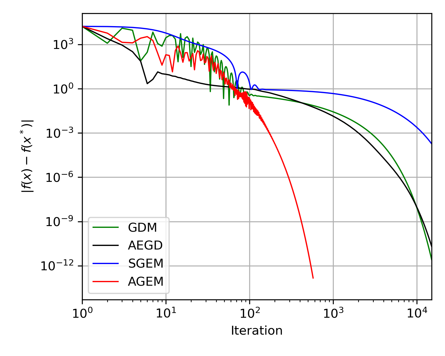
Figure 1. Comparison of the performance of different methods on the 2D Rosenbrock function $f(x_{1},x_{2})=(1-x_{1})^{2}+100(x_{2}-x_{1}^{2})^{2}$.

The main objective of this work is to present a detailed analysis of AGEM using both its discrete and continuous formulations. These results are expected to also hold true for (2.2).

We are particularly interested in the convergence properties of AGEM. This will be studied from the perspective of continuous dynamics for general smooth objective functions. Furthermore, based on a structural condition on $f$ – the so-called Polyak-Łojasiewicz (PL) condition, we derive a convergence rate in Section 6.

2.2. PL condition for non-convex objectives

Here we present a short account on the PL condition and its relevance to the loss function in the context of deep neural networks.

Definition 2.3.

For a differentiable function $f:\mathbb{R}^{n}\to\mathbb{R}$ with ${\rm argmin}f(\theta)\neq\emptyset$, we say $f$ satisfies the PL condition if there exists some constant $\mu>0$, such that the following inequality holds for any $\theta^{*}\in{\rm argmin}f(\theta)$:

(2.6) $$\frac{1}{2}|\nabla f(\theta)|^{2}\geq\mu(f(\theta)-f(\theta^{*})),\quad\forall\theta\in\mathbb{R}^{n}.$$

This means that a local minimizer $\theta^{*}$ is also a global minimizer. We note that strongly convex functions satisfy the PL condition, while a function that satisfies the PL condition is not necessary to be convex. For example, the function

$$f(\theta)=\theta^{2}+3\sin^{2}\theta$$

is not convex but satisfies the PL condition with $\mu=\frac{1}{32},f^{*}=0$.

As we mentioned in the introduction, PL condition has attracted increasing attention in connection with the convergence of training deep neural network tasks. Here we conduct an informal investigation on how a loss function commonly used in training deep learning tasks can satisfy the PL condition. Consider the following loss function

$$f(\theta):=\frac{1}{2}\sum_{i=1}^{m}(g(x_{i};\theta)-y_{i})^{2},$$

with $f(\theta^{*})=0$ for any minimizer $\theta^{*}$. Here $\{x_{i},y_{i}\}_{i=1}^{m}$ are training data points, $g$ is a deep neural network prediction parameterized by $\theta$. The gradient of such loss function is

$$\nabla f(\theta)=\sum_{i=1}^{m}(g(x_{i};\theta)-y_{i})\frac{\partial g(x_{i};\theta)}{\partial\theta}.$$

Denoting $u=(u_{1},...,u_{m})$ where $u_{i}=g(x_{i};\theta)-y_{i}$, we have

(2.7) $$\frac{1}{2}|\nabla f(\theta)|^{2}=\frac{1}{2}\sum_{i=1}^{m}\sum_{j=1}^{m}u_{i}H_{ij}u_{j}=\frac{1}{2}uHu^{\top},$$

where $H$ is a $m\times m$ matrix with $(i,j)$ entry defined by

(2.8) $$H_{ij}=\langle\frac{\partial g(x_{i};\theta)}{\partial\theta},\frac{\partial g(x_{j};\theta)}{\partial\theta}\rangle.$$

From (2.7) it can be seen that as long as the smallest eigenvalue of $H$ is lower bounded by $\mu$, we have

$$\frac{1}{2}|\nabla f(\theta)|^{2}\geq\frac{1}{2}\mu|u|^{2}=\mu f(\theta).$$

This is indeed the PL condition. In fact, using over-parameterization and random initialization, [15] has proved that for a two-layer neural network with rectified linear unit (ReLU) activation, the smallest eigenvalue of $H$ is indeed strictly positive and it plays an essential role in deriving the linear convergence rate of gradient descent in [15]. A similar convergence result for implicit networks is also obtained in [17].

3. Solution properties of the AGEM algorithm

In this section, we establish that the iterates generated by (2.3) are uniformly bounded and convergent if $\eta$ is suitably small.

Theorem 3.1.

Under Assumption 2.1, for $(\theta_{k},r_{k},v_{k})$ generated by (2.3), if $\eta<\eta^{*}$ for some $\eta^{*}>0$, we have the following results:

1. (Uniformly boundedness) $\theta_{k}$ and $v_{k}$ are bounded for all $k\geq 1$. Moreover,

   $$\theta_{k}\in\{\theta\in\mathbb{R}^{n}\;|\;F(\theta)\leq 2F(\theta_{0})\},\quad|v_{k}|\leq\max_{j\leq k}|\nabla F(\theta_{j})|.$$

2. (Lower bound on energy) The lower bound of $r_{k}$ is strictly positive:

   $$r_{k}\geq r_{k+1}\geq r^{*}>0,\quad\forall k\geq 0.$$

3. (Convergence) As $k\to\infty$, we have

   $$r_{k}\to r^{*}>0,\quad v_{k}\to 0,\quad\nabla f(\theta_{k})\to 0.$$

Proof.

Define

(3.1) $$Q_{k}:=F(\theta_{k})+\epsilon r_{k}|v_{k-1}|^{2},$$

where $\epsilon=\frac{\eta\beta}{1-\beta}$, then we claim:

(3.2) $$Q_{k+1}-Q_{k}\leq-\epsilon r_{k+1}|v_{k}-v_{k-1}|^{2}-2\eta r_{k+1}|v_{k}|^{2}+\frac{L_{F}(\theta_{k+\frac{1}{2}})}{2}|\theta_{k+1}-\theta_{k}|^{2},$$

where $L_{F}(\theta_{k+\frac{1}{2}})$ is the largest eigenvalue of $\max_{s\in[0,1]}D^{2}F((1-s)\theta_{k}+s\theta_{k+1})$. In fact,

(3.3) $$Q_{k+1}-Q_{k}=F(\theta_{k+1})-F(\theta_{k})+\epsilon r_{k+1}|v_{k}|^{2}-\epsilon r_{k}|v_{k-1}|^{2},$$

where

(3.4) $$F(\theta_{k+1})-F(\theta_{k})\leq\langle\nabla F(\theta_{k}),\theta_{k+1}-\theta_{k}\rangle+\frac{L_{F}(\theta_{k+\frac{1}{2}})}{2}|\theta_{k+1}-\theta_{k}|^{2},$$

in which,

(3.5) $$\quad\langle\nabla F(\theta_{k}),\theta_{k+1}-\theta_{k}\rangle$$

$$=-2\eta r_{k+1}\langle\nabla F(\theta_{k}),v_{k}\rangle$$

$$=-2\eta r_{k+1}\langle\nabla F(\theta_{k})-v_{k},v_{k}\rangle-2\eta r_{k+1}|v_{k}|^{2}$$

$$=-2\eta r_{k+1}\langle\frac{\beta}{1-\beta}(v_{k}-v_{k-1}),v_{k}\rangle-2\eta r_{k+1}|v_{k}|^{2}$$

$$=-\epsilon r_{k+1}(|v_{k}|^{2}-|v_{k-1}|^{2}+|v_{k}-v_{k-1}|^{2})-2\eta r_{k+1}|v_{k}|^{2}$$

$$\leq-\epsilon r_{k+1}|v_{k}|^{2}+\epsilon r_{k}|v_{k-1}|^{2}-\epsilon r_{k+1}|v_{k}-v_{k-1}|^{2}-2\eta r_{k+1}|v_{k}|^{2},$$

where $r_{k+1}<r_{k}$ is used in the last inequality. Connecting (3.3), (3.4), (3.5) gives (3.2).

(1) To show the uniformly boundedness, we take a summation on (3.2) from $0$ to $k$ and ignore the negative terms on the RHS to have

(3.6) $$Q_{k+1}\leq Q_{0}+\frac{\max_{j\leq k}L_{F}(\theta_{j+\frac{1}{2}})}{2}\sum_{j=0}^{k}|\theta_{j+1}-\theta_{j}|^{2}.$$

Using $Q_{0}=F(\theta_{0})$ and the bound in (2.5), we further get

(3.7) $$F(\theta_{k+1})\leq F(\theta_{0})+\frac{1}{2}\eta r^{2}_{0}\max_{j\leq k}L_{F}(\theta_{j+\frac{1}{2}}).$$

Now we show if $\eta$ is suitably small, $\{\theta_{k}\}$ is uniformly bounded. This further ensures the boundedness of $\{v_{k}\}$, since

(3.8) $$|v_{k}|\leq(1-\beta)\sum_{j=0}^{k}\beta^{k-j}|\nabla F(\theta_{j})|\leq\max_{j\leq k}|\nabla F(\theta_{j})|.$$

To proceed, we use the notation:

$$\Sigma_{k}:=\{\theta\in\mathbb{R}^{n}\;|\;F(\theta)\leq kF(\theta_{0})\},\quad k=2,3$$

and $\tilde{\Sigma}_{k}$ for the convex hull of $\Sigma_{k}$. By the assumption, $\Sigma_{2}\subset\Sigma_{3}$ are bounded domains. We want to identify conditions on $\eta$ such that $\{\theta_{k}\}\in\Sigma_{2}$ for all $k\geq 1$. This can be carried out by induction. Obviously $\theta_{0}\in\Sigma_{2}$. It suffices to show that under suitable conditions on $\eta$, we have

$$\{\theta_{j}\}_{j\leq k}\subset\Sigma_{2}\Rightarrow\theta_{k+1}\in\Sigma_{2}$$

The main task here is to find the a sufficient condition on $\eta$, for which we argue in two steps:

(i) By continuity of $F$, there exists $\delta_{F}(r_{0})$ such that if

(3.9) $$|\theta_{k+1}-\theta_{k}|<\delta_{F}(r_{0}),$$

we have

$$|F(\theta_{k+1})-F(\theta_{k})|<r_{0}.$$

This implies $F(\theta_{k+1})\leq F(\theta_{k})+r_{0}\leq 3r_{0}$, that is $\theta_{k+1}\in\Sigma_{3}.$ On the other hand,

$$|\theta_{k+1}-\theta_{k}|=|-2\eta r_{k+1}v_{k}|\leq 2\eta r_{0}\max_{j\leq k}|\nabla F(\theta_{j})|\leq 2\eta r_{0}\max_{\theta\in\Sigma_{2}}|\nabla F(\theta)|.$$

This ensures (3.9) if we take

$$\eta<\eta_{1}:=\frac{\delta_{F}(r_{0})}{2r_{0}\max_{\theta\in\Sigma_{2}}|\nabla F(\theta)|}.$$

(ii) Note that $\theta_{k+1}\in\Sigma_{3}$ and $\{\theta_{j}\}_{j\leq k}\in\Sigma_{2}\subset\Sigma_{3}$, we have $\{\theta_{j+\frac{1}{2}}\}_{j\leq k}\subset\tilde{\Sigma}_{3}$. By (3.7),

(3.10) $$F(\theta_{k+1})\leq F(\theta_{0})+\frac{1}{2}\eta r^{2}_{0}\max_{\theta\in\tilde{\Sigma}_{3}}L_{F}(\theta).$$

This gives

$$F(\theta_{k+1})\leq 2F(\theta_{0}),$$

provided

$$\eta\leq\eta_{2}:=\frac{2}{r_{0}\max_{\theta\in\tilde{\Sigma}_{3}}L_{F}(\theta)}.$$

Hence $\theta_{k+1}\in\Sigma_{2}$. We conclude that if $\eta<\min\{\eta_{1},\eta_{2}\}$, then $\theta_{k}\in\Sigma_{2}$ for all $k$.

(2) Theorem 2.2 states that $r_{k}\to r^{*}\geq 0$ as $k\to\infty$. Here we identify a sufficient condition on $\eta$, so that $r^{*}>0$ is guaranteed. Following the same argument as in (1), while keeping one negative term

$$-2\eta r_{k+1}|v_{k}|^{2}=r_{k+1}-r_{k},$$

on the RHS of (3.2), we obtain

$$F(\theta_{k})\leq F(\theta_{0})+r_{k}-r_{0}+\frac{1}{2}\eta r_{0}^{2}\max_{\theta\in\tilde{\Sigma}_{3}}L_{F}(\theta),$$

under the condition that $\eta<\eta_{1}$. Since $r_{0}=F(\theta_{0})$, we have

$$r_{k}\geq F(\theta_{k})-\frac{1}{2}\eta r_{0}^{2}\max_{\theta\in\tilde{\Sigma}_{3}}L_{F}(\theta).$$

Let $k\to\infty$, then

$$r^{*}\geq\liminf_{k\to\infty}F(\theta_{k})-\frac{1}{2}\eta r_{0}^{2}\max_{\theta\in\tilde{\Sigma}_{3}}L_{F}(\theta)\geq F^{*}-\frac{1}{2}\eta r_{0}^{2}\max_{\theta\in\tilde{\Sigma}_{3}}L_{F}(\theta)>0,$$

provided

$$\eta\leq\eta_{3}:=\frac{2F^{*}}{r^{2}_{0}\max_{\theta\in\tilde{\Sigma}_{3}}L_{F}(\theta)}.$$

That is, if $\eta<\min\{\eta_{1},\eta_{3}\}$, then $r^{*}>0$. Note that $\eta_{3}\leq\eta_{2}$, thus both (1) and (2) are satisfied if we take $\eta<\eta^{*}:=\min\{\eta_{1},\eta_{3}\}$.

(3) Recall in Theorem 2.2 we have shown that $|\theta_{k+1}-\theta_{k}|\to 0$. Using (2.3), we get

$$r_{k+1}|v_{k}|\to 0.$$

By (2), $r_{k}\to r^{*}>0$ when $\eta<\eta^{*}$. Thus $|v_{k}|\to 0$ must hold. By (2.3a), this further implies $\nabla F(\theta_{k})\to 0$, hence $\nabla f(\theta_{k})=2F(\theta_{k})\nabla F(\theta_{k})\to 0$ holds as well.

∎

Remark 3.2.

If $f$ is assumed to be $L$-smooth, then $L_{F}$ is uniformly bounded. In such case, the boundedness of the solution is achieved without any restriction on $\eta$, as can be seen from $(\ref{Qr})$. However, the $L$-smoothness assumption would exclude a large class of objective functions such as $|\theta|^{4}$.

4. Discrete to continuous-time-limits

Scheme (2.3) can be studied by considering the limiting ODEs obtained by taking the step size $\eta\to 0$. However, different ODEs can be obtained when the hyper-parameters are scaled differently. Here we shall derive an ODE system which keeps certain momentum effects.

For any $k\geq 0$, let $t_{k}=k\eta$, and assume $v_{k}=v(t_{k}),r_{k}=r(t_{k}),\theta_{k}=\theta(t_{k})$ for some sufficiently smooth curve $(v(t),r(t),\theta(t))$. Performing the Taylor expansion on $v_{k-1}$ in powers of $\eta$, we get

$$v_{k-1}=v(t_{k-1})=v(t_{k})-\eta\dot{v}(t_{k})+O(\eta^{2}).$$

Substituting $v_{k-1}$ into (2.3a), we have

$$v(t_{k})=\beta(v(t_{k})-\eta\dot{v}(t_{k})+O(\eta^{2}))+(1-\beta)\nabla F(\theta(t_{k})),$$

which gives

(4.1) $$\frac{\beta\eta}{1-\beta}\dot{v}=-v+\nabla F(\theta)+O(\eta^{2}),\quad\text{at}\;t=t_{k}.$$

Plugging $r_{k+1}=r(t_{k})+\eta\dot{r}(t_{k})+O(\eta^{2})$ in (2.3b) we have

(4.2) $$\dot{r}=-\frac{2r|v|^{2}}{1+2\eta|v|^{2}}+O(\eta^{2}),\quad\text{at}\;t=t_{k}.$$

Similarly, from (2.3c) we have

(4.3) $$\dot{\theta}=-\frac{2rv}{1+2\eta|v|^{2}}+O(\eta^{2}),\quad\text{at}\;t=t_{k}.$$

We first discard $O(\eta^{2})$ and keep $O(\eta)$ terms in (4.1) (4.2), (4.3), which leads to the following ODE system:

(4.4a) $$\epsilon\dot{v} =-v+\nabla F(\theta),$$

(4.4b) $$\dot{r} =-\frac{2r|v|^{2}}{1+2\eta|v|^{2}},$$

(4.4c) $$\dot{\theta} =-\frac{2rv}{1+2\eta|v|^{2}},$$

where $\epsilon=\frac{\beta\eta}{1-\beta}$. This can be viewed as a high-resolution ODE [33] because of the presence of $O(\eta)$ terms.

Let $\eta\to 0$, then (4.4) reduces to the following ODE system:

(4.5a) $$\dot{r} =-2r|\nabla F(\theta)|^{2},$$

(4.5b) $$\dot{\theta} =-2r\nabla F(\theta).$$

From two equations in (4.5) together with $r(0)=F(\theta_{0})$ we can show

$$r(t)=F(\theta(t)),\quad\forall t>0,$$

with which, (4.5b) reduces to

(4.6) $$\dot{\theta}=-2F(\theta)\nabla F(\theta)=-\nabla f(\theta).$$

This says that the ODE system (4.5) is equivalent to the gradient flow (4.6).

To study the momentum effect, we keep $\epsilon=\frac{\beta\eta}{1-\beta}$ unchanged while letting $\eta\to 0$. This way, we obtain the following system of ODEs:

(4.7a) $$\epsilon\dot{v} =-v+\nabla F(\theta),$$

(4.7b) $$\dot{r} =-2r|v|^{2},$$

(4.7c) $$\dot{\theta} =-2rv.$$

Compared with (4.7), the high-resolution ODEs (4.4) are more accurate continuous-time counterparts for the corresponding discrete algorithm (2.3). While the analysis of (4.4) would be more involved. In the rest of this work, we focus on (4.7) and provide a detailed analysis of it.

Theorem 4.1.

Denote $U_{k}=(\theta_{k},v_{k},r_{k})$ as the solution given in Theorem 3.1, $U(t)=(\theta(t),v(t),r(t))$ as the solution to (4.7), then for any $T>0$, we have

$$\lim_{\begin{subarray}{c}\eta\to 0\\ k\eta=T\end{subarray}}U_{k}=U(T).$$

This result follows from a standard ODE analysis. In the present setting, it is guaranteed by the boundedness of $U_{k}$ as shown in Theorem 3.1 and the boundedness of $U(t)$ that will be shown in Theorem 5.1.

5. Dynamic solution behavior

This section is devoted to the analysis of (4.7), including global existence, asymptotic convergence to equilibria using the celebrated LaSalle invariance principle [23], as well as convergence rates for non-convex objective functions satisfying the PL property.

5.1. Global Existence and Uniqueness

Theorem 5.1.

Under Assumption 2.1, the ODE (4.7) with initial condition $(\theta_{0},r_{0}>0,v_{0})$ has a unique global solution $(\theta(t),v(t),r(t))\in C^{1}([0,\infty];\mathbb{R}^{2n+1})$. In particular, for any $t>0$, we have

(5.1) $$\theta(t)\in\{\theta\in\mathbb{R}^{n}\;|\;F(\theta)\leq F(\theta_{0})+\epsilon r_{0}|v_{0}|^{2}\},$$

$$|v(t)|\leq\max\{|v(0)|,\max_{[0,t]}|\nabla F(\theta(\cdot))|\},$$

$$0<r(t)\leq r_{0}.$$

Proof.

For $f\in C^{1}(\mathbb{R}^{n})$, due to Picard and Lindelöf, there exists a unique local solution to (4.7) with initial condition $(\theta_{0},r_{0},v_{0})$. According to the extension theorem, the only way in which global existence can fail is if the solution ‘escapes’ to infinity. Hence, to establish the global existence, it suffices to show $(\theta(t),r(t),v(t))$ remains bounded for all $t>0$. To do this, we introduce a suitable control function. A candidate based on the discrete counterpart is

(5.2) $$Q:=Q(\theta,r,v)=F(\theta)+\epsilon r|v|^{2}.$$

Using the chain rule, we find that if $(\theta,r,v)$ satisfies (4.7), then

(5.3) $$\dot{Q} =\langle\nabla F(\theta),\dot{\theta}\rangle+\epsilon\dot{r}|v|^{2}+2\epsilon r\langle v,\dot{v}\rangle$$

$$=-2r\langle\nabla F(\theta),v\rangle-2\epsilon r|v|^{4}+2r\langle v,-v+\nabla F(\theta)\rangle$$

$$=-2r|v|^{2}-2\epsilon r|v|^{4}\leq 0.$$

Hence $Q$ is guaranteed to decrease. In particular, we have

(5.4) $$F(\theta)+\epsilon r|v|^{2}\leq Q(\theta_{0},r_{0},v_{0}),$$

which implies the boundedness of $F(\theta)$. This together with the coerciveness of $f$, hence of $F$, guarantees that $\theta(t)$ is bounded for all $t>0$. But the above inequality does not give us an uniform bound for $v(t)$.

To seek a useful bound for $v(t)$, we shall use (4.7a):

$$\partial_{t}v+\frac{1}{\epsilon}v=\frac{1}{\epsilon}\nabla F(\theta(t)),$$

which gives

$$\frac{d}{dt}(v(t)e^{t/\epsilon})=\frac{1}{\epsilon}e^{t/\epsilon}\nabla F(\theta(t)).$$

So for every $t$, we have

$$v(t)=v(0)e^{-t/\epsilon}+\frac{1}{\epsilon}\int_{0}^{t}e^{(\tau-t)/\epsilon}\nabla F(\theta(\tau))d\tau.$$

Hence

$$|v(t)| \leq|v(0)|e^{-t/\epsilon}+(1-e^{-t/\epsilon})\max_{\tau\in[0,t]}|\nabla F(\theta(\tau))|$$

$$\leq\max\{|v(0)|,\max_{\tau\in[0,t]}|\nabla F(\theta(\tau))|\}.$$

Note that the boundedness of $\nabla F(\theta(t))$ is ensured by

$$|\nabla F(\theta(t))|=\bigg{|}\frac{\nabla f(\theta(t))}{2F(\theta(t))}\bigg{|}\leq\bigg{|}\frac{\nabla f(\theta(t))}{2F^{*}}\bigg{|}.$$

From (4.7), we see that $r$ decreases monotonically, thus $0\leq r(t)\leq r_{0}$. This concludes the proof.

∎

Remark 5.2.

The uniform boundedness of $|v|$ validates the removal of $2\eta|v|^{2}$ in (4.4b) and (4.4c) while passing limit $\eta\to 0$.

5.2. Asymptotic behavior of solutions

Theorem 5.3.

Under Assumption 2.1, let $(\theta(t),r(t),v(t))$ be the global solution to the ODE (4.7) as stated in Theorem 5.1 with initial condition $(\theta_{0},r_{0},v_{0})$. If

(5.5) $$r_{0}>F(\theta_{0})-F^{*},\quad\epsilon|v_{0}|^{2}<1-\frac{F(\theta_{0})-F^{*}}{r_{0}},$$

then as $t\to\infty$,

$$\nabla F(\theta(t))\rightarrow 0,\quad r(t)\rightarrow r^{*}>0,\quad v(t)\rightarrow v^{*}=0.$$

Moreover, $F(\theta(t))\rightarrow F^{*}$ a minimum value of $F$, and

(5.6) $$r^{*}<r(t)\leq r_{0},\quad F^{*}\leq F(\theta(t))\leq F(\theta_{0})+\epsilon r_{0}|v_{0}|^{2}.$$

The upper bound on $F$ follows directly from (5.4). We prove the convergence result in three steps.

Step 1. We show $r^{*}:=\lim_{t\to\infty}r(t)$ exists and $r^{*}>0$.
First, since $\dot{r}\leq 0$ and $r\geq 0$, hence $\int_{0}^{\infty}|\dot{r}|dt\leq r_{0}<\infty$, this ensures that $\lim_{t\to\infty}r(t)=r^{*}$ exists. Note that (5.3) can be written as

$$\dot{r}=\dot{Q}+2\epsilon r|v|^{4}.$$

Integrating on both sides from $0$ to $t$ and using (5.5), we have

(5.7) $$r(t) =r_{0}+F(\theta(t))+\epsilon r(t)|v(t)|^{2}-(F(\theta_{0})+\epsilon r_{0}|v_{0}|^{2})+2\epsilon\int_{0}^{t}r|v|^{4}ds$$

$$\geq r_{0}-(F(\theta_{0})-F^{*})-\epsilon r_{0}|v_{0}|^{2}>0.$$

From this lower bound, we obtain

$$r^{*}=\lim_{t\to\infty}r(t)\geq r_{0}+F^{*}-F(\theta_{0})-\epsilon r_{0}|v_{0}|^{2}>0.$$

Step 2. We proceed to analyze the asymptotic behavior of $\theta$ and $v$ by using LaSalle’s invariance principle [23]. Recall the function $Q$ defined in Theorem 5.1,

$$Q(\theta,r,v)=F(\theta)+\epsilon r|v|^{2}.$$

This form and the fact $r(t)\geq r^{*}>0$ implies that

$$\Omega=\{(\theta,r,v)\;|\;Q(\theta,r,v)\leq Q(\theta_{0},r_{0},v_{0})\}$$

is a compact positively invariant set with respect to (4.7), and for any $(\theta,r,v)\in\Omega$,

$$\dot{Q}(\theta,r,v)=-2r|v|^{2}-2\epsilon r|v|^{4}\leq 0.$$

Define the set

$$\Sigma=\{(\theta,r,v)\in\Omega\;|\;\dot{Q}(\theta,r,v)=0\},$$

since $r(t)\geq r^{*}>0$ for all $t>0$, thus

$$\Sigma=\{(\theta,r,v)\in\Omega\;|\;r|v|=0\}=\{(\theta,r,v)\in\Omega\;|\;v=0,r\geq r^{*}\}.$$

Next we identify the largest invariant set in $\Sigma$. Suppose that at some $t_{1}$, $v(t_{1})=0$, then we have $\dot{\theta}=0,\dot{r}=0$, but $\epsilon\dot{v}(t_{1})=\nabla F(\theta(t_{1}))$. As a result, the trajectory will not stay in $\Sigma$ unless $\nabla F(\theta(t_{1}))=0$. That is, the largest invariant set in $\Sigma$ must be

$$\Sigma_{0}=\{(\theta,r,v)\in\Omega\;|\;v=0,\nabla F(\theta)=0,r\geq r^{*}\}.$$

By LaSalle’s invariance principle, every trajectory of (4.7) starting in $\Omega$ tends to $\Sigma_{0}$ as $t\to\infty$. From Step 1, $r^{*}$ is the only limit of $r(t)$. Hence then all trajectories will admit a limit or a cluster point in

$$\{(\theta,r^{*},0)\;|\;\nabla F(\theta)=0\}.$$

That is, we have $\lim_{t\to\infty}\nabla F(\theta(t))=0$. Note that $Q$ is monotone and bounded, hence admitting a limit $b>0$. This further implies that the following

$$\lim_{t\to\infty}F(\theta(t))=\lim_{t\to\infty}[Q(\theta(t),r(t),v(t))-\epsilon r(t)|v(t)|^{2}]=b\geq\inf F.$$

Step 3. Finally, we show $b$ is a local minimum value of $F$, rather than a local maximum value. We prove this by contradiction. Suppose $b$ is a local maximum value of $F$. Recall that $F(\theta)\to b$, $r\to r^{*}$ and $|v|\to 0$ as $t\to\infty$, thus for any $\delta>0$, there exists $t_{1}=t_{1}(\delta)$ such that for any $t\geq t_{1}$,

$$|F(\theta(t))-b|\leq\delta,\quad|r(t)-r^{*}|\leq\delta,\quad|v(t)|\leq\delta.$$

Since $F$ is continuous, there exists $t_{2}\geq t_{1}$ such that

$$F(\theta(t_{2}))\leq b-\frac{\delta}{2},$$

where we have used the assumption that $b$ is a local maximum value of $F$. From Step 2, we know that $Q$ is non-increasing in $t$, hence for any $t\geq t_{2}$, we have

$$Q(t)\leq Q(t_{2})=F(\theta(t_{2}))+\epsilon r(t_{2})|v(t_{2})|^{2}\leq b-\frac{\delta}{2}+\epsilon(r^{*}+\delta)\delta^{2}<b,$$

provided $\delta$ is small so that $(r^{*}+\delta)\delta<\frac{1}{2\epsilon}$. Now letting $t\to\infty$,we have $b=\lim_{t\to\infty}Q(t)<b$. This is a contradiction. Hence $b$ has to be a local minimum value of $F$, i.e., $b=F^{*}$.

6. Convergence rate

How fast the solution can converge to the minimal value of $f$ depends on the geometry of the objective function near $f^{*}$. Indeed, under the PL condition, we can show the $f(\theta(t))$ can reach $f^{*}$ exponentially fast.

Theorem 6.1.

Let $(\theta(t),r(t),v(t))$ be the global solution to (4.7) as stated in Theorem 5.3 with initial condition $(\theta_{0},r_{0},v_{0})=(\theta_{0},F(\theta_{0}),0)$. Suppose $f$ also satisfies the PL condition (2.6) with $\mu>0$, then for any $\delta\in(0,1)$, the following bounds hold

(6.1) $$f(\theta(t))-f^{*}\leq(f(\theta_{0})-f^{*})\bigg{(}e^{-\frac{2\mu r^{*}}{F(\theta_{0})(2-\delta)}t}+\frac{2\mu\epsilon}{\delta(2-\delta)}e^{-\frac{\delta}{\epsilon}t}\bigg{)}$$

provided that $\epsilon\leq\min\{\epsilon_{1},\epsilon_{2}\}$ where

(6.2) $$\epsilon_{1}=\delta(1-\delta)\frac{F^{*}}{2LF(\theta_{0})},\quad\epsilon_{2}=\frac{1}{2\mu F(\theta_{0})}(2-\delta)(1-\delta)\bigg{(}F(\theta_{0})+\frac{F^{*}r^{*}}{F(\theta_{0})}\bigg{)}.$$

Here $L$ is the the largest eigenvalue of $D^{2}f(\theta)$, where $\theta$ is in the solution domain in Theorem 5.1.

Remark 6.2.

Observe from (6.1) that for small $\epsilon$ the convergence rate would be dominated by $e^{-\frac{2\mu r^{*}}{F(\theta_{0})(2-\delta)}t}$. More precisely, we have

$$f(\theta(t))-f^{*}\leq(f(\theta_{0})-f^{*})\bigg{(}e^{-\frac{2\mu r^{*}}{F(\theta_{0})(2-\delta)}t}\bigg{)},$$

if $\epsilon\leq\{\epsilon_{1},\epsilon_{2},\epsilon_{3}\}$ with $\epsilon_{3}=\frac{F(\theta_{0})\delta(2-\delta)}{2\mu r^{*}}$. Also $\frac{2\mu r^{*}}{F(\theta_{0})(2-\delta)}$ gets larger as $\delta\to 1$. For $\delta=1$, $\epsilon$ is forced to be $0$, then (4.7) reduces to (4.5) or (4.6). In such case, $\frac{2\mu r^{*}}{F(\theta_{0})(2-\delta)}$ becomes $2\mu$, which recovers the convergence rate of gradient flow (4.6) under the PL condition [31].

The proof presented below is in three steps:

1. We introduce a candidate control function,

   $$E=a(f(\theta)-f^{*})-\epsilon\langle\nabla f(\theta),v\rangle+\lambda\epsilon r|v|^{2},$$

   with parameters $a,\lambda>0$ to be determined.

2. We identify admissible pairs $(a,\lambda)$ such that $E(t)$ decays exponentially fast.

3. Using $\dot{W}(t)=\langle\nabla f(\theta),\dot{\theta}\rangle=-2r\langle\nabla f(\theta),v\rangle$, we link $E$ to $W:=f(\theta)-f^{*}$ by

   (6.3) $$E=aW+\frac{\epsilon\dot{W}}{2r}+\lambda\epsilon r|v|^{2},$$

   and derive the convergence rate of $W$ based on the convergence rate of $E$.

Proof.

Step 1: Decay of the control function. Define

(6.4) $$E=a(f(\theta)-f^{*})-\epsilon\langle\nabla f(\theta),v\rangle+\lambda\epsilon r|v|^{2},$$

where parameters $a,\lambda>0$ will be determined later so that along the trajectory of (4.7) $E=E(t)$ has an exponential decay rate.

For each term in $E$ we proceed to evaluate their time derivative along the trajectory of (4.7). For the first term, we get

$$\frac{d}{dt}(f(\theta)-f^{*})=\langle\nabla f(\theta),\dot{\theta}\rangle=-2r\langle\nabla f(\theta),v\rangle.$$

For the second term, we have

$$\frac{d}{dt}\epsilon\langle\nabla f(\theta),v\rangle =\epsilon\langle\nabla^{2}f(\theta)\dot{\theta},v\rangle+\epsilon\langle\nabla f(\theta),\dot{v}\rangle$$

(6.5) $$=-2\epsilon r\langle\nabla^{2}f(\theta)v,v\rangle-\langle\nabla f(\theta),v\rangle+\langle\nabla f(\theta),\nabla F(\theta)\rangle.$$

Note that

$$\langle\nabla^{2}f(\theta)v,v\rangle\leq L|v|^{2},\quad\text{and}$$

$$\langle\nabla f(\theta),\nabla F(\theta)\rangle=\frac{1}{2F(\theta)}|\nabla f(\theta)|^{2}\geq\frac{\mu}{F(\theta)}(f(\theta)-f^{*}).$$

Here we used $\nabla F(\theta)=\nabla f(\theta)/(2F(\theta))$ and the PL property for $f$.

Hence (6.5) reduces to

$$\frac{d}{dt}\epsilon\langle\nabla f(\theta),v\rangle\geq-2\epsilon Lr|v|^{2}-\langle\nabla f(\theta),v\rangle+\frac{\mu}{F(\theta)}(f(\theta)-f^{*}).$$

For the third term, we have

$$\frac{d}{dt}\epsilon r|v|^{2} =\epsilon\dot{r}|v|^{2}+2\epsilon r\langle v,\dot{v}\rangle$$

$$=-2\epsilon r|v|^{4}+2r\langle v,-v+\nabla F(\theta)\rangle$$

$$=-2\epsilon r|v|^{4}-2r|v|^{2}+2r\langle\nabla F(\theta),v\rangle$$

$$\leq-2r|v|^{2}+\frac{r}{F(\theta)}\langle\nabla f(\theta),v\rangle.$$

Combining the above three estimates together we obtain

(6.6) $$\dot{E}(t)\leq-\frac{\mu}{F(\theta)}(f(\theta)-f^{*})+(2\epsilon L-2\lambda)r|v|^{2}+\bigg{(}-2ar+1+\frac{\lambda r}{F(\theta)}\bigg{)}\langle\nabla f(\theta),v\rangle.$$

Note that (6.4) can be rewritten as

(6.7) $$\langle\nabla f(\theta),v\rangle=\frac{a}{\epsilon}(f(\theta)-f^{*})+\lambda r|v|^{2}-\frac{1}{\epsilon}E(t).$$

This upon substitution into (6.6) gives

(6.8) $$\dot{E}(t)\leq-\frac{b(t)}{\epsilon}E(t)+\left(\frac{ab(t)}{\epsilon}-\frac{\mu}{F(\theta)}\right)(f(\theta)-f^{*})+(\lambda b(t)+2\epsilon L-2\lambda)r|v|^{2},$$

where $b(t):=-2ar(t)+1+\frac{\lambda r(t)}{F(\theta(t))}$. This leads to

(6.9) $$\dot{E}(t)\leq-\frac{b(t)}{\epsilon}E(t),$$

as long as we can identify $a,\lambda$ so that

(6.10a) $$b(t)=-2ar(t)+1+\frac{\lambda r(t)}{F(\theta(t))}>0,$$

(6.10b) $$\frac{ab(t)}{\epsilon}-\frac{\mu}{F(\theta(t))}\leq 0,$$

(6.10c) $$\lambda b(t)+2\epsilon L-2\lambda\leq 0,$$

for all $t>0$.

Step 2: Admissible choice for $\lambda,a$. Using the solution bounds $r^{*}\leq r(t)\leq r_{0}$ and $F^{*}\leq F(\theta(t))\leq F(\theta_{0})$, we have

$$b_{*}\leq b(t)\leq b^{*},\quad\forall t>0,$$

where

$$b_{*}=b_{*}(a,\lambda)=-2ar_{0}+1+\frac{\lambda r_{*}}{F(\theta_{0})},$$

$$b^{*}=b^{*}(a,\lambda)=-2ar^{*}+1+\frac{\lambda r_{0}}{F^{*}}.$$

In order to ensure (6.10c) we must have $b^{*}<2$. Putting these together, condition (6.10) can be ensured by the following stronger constraints:

(6.11a) $$0<b_{*},\quad b^{*}<2,$$

(6.11b) $$ab^{*}-\frac{\epsilon\mu}{F(\theta_{0})}\leq 0,$$

(6.11c) $$\lambda b^{*}+2\epsilon L-2\lambda\leq 0.$$

A direct calculation shows that for small $\epsilon$, such admissible pair exists, with $a=O(\epsilon)$, and $\lambda\leq\frac{F^{*}}{r_{0}}$ which is induced from $b^{*}<2$. To be more precise, we fix $\delta\in(0,1)$ and require that

$$b_{*}\geq\delta.$$

The constraint $b^{*}<2$ would impose a lower bound for $a\sim\epsilon$ (which we should avoid to stay consistency with the discrete algorithm) unless $\lambda$ is chosen to satisfy $b^{*}+2ar^{*}\leq 2-\delta$. This is equivalent to requiring

$$\lambda\leq(1-\delta)\frac{F^{*}}{r_{0}}.$$

With the above two constraints, it is safe to replace $b^{*}$ by $2-\delta$ in (6.11b) and (6.11c), respectively, so that

(6.12) $$a(2-\delta)\leq\frac{\epsilon\mu}{F(\theta_{0})},\quad 2\epsilon L\leq\delta\lambda.$$

The convergence rate estimate in the next step requires $a$ to be large as possible, we thus simply take

(6.13) $$a=\frac{\epsilon\mu}{F(\theta_{0})(2-\delta)}.$$

The second relation in (6.12) now reduces to

$$\epsilon\leq\frac{\delta\lambda}{2L}.$$

Note that the constraint $b_{*}\geq\delta$ is met if $2ar_{0}\leq 1-\delta+\frac{\lambda r^{*}}{F(\theta_{0})}$, imposing another upper bound on $\epsilon$. To be concrete, we take

(6.14) $$\lambda=(1-\delta)\frac{F^{*}}{r_{0}},$$

then (6.11) is met if

$$\epsilon\leq\min\{\epsilon_{1},\epsilon_{2}\},$$

with

$$\epsilon_{1}=\delta(1-\delta)\frac{F^{*}}{2Lr_{0}},\quad\epsilon_{2}=\frac{1}{2\mu r_{0}}(2-\delta)(1-\delta)\bigg{(}F(\theta_{0})+\frac{F^{*}r^{*}}{r_{0}}\bigg{)}.$$

This is (6.2) with $r_{0}=F(\theta_{0})$. Hence, for suitably small $\epsilon$, we have obtained a set of admissible pairs $(a,\lambda)$ with

(6.15) $$a=\frac{\epsilon\mu}{F(\theta_{0})(2-\delta)},\quad\lambda=(1-\delta)\frac{F^{*}}{r_{0}},$$

as $\delta$ varies in $(0,1)$.

Step 3: Convergence rate of $W$. With above choices of $(a,\lambda)$, we have

(6.16) $$\dot{E}(t)\leq-\frac{b(t)}{\epsilon}E(t)\leq-\frac{b_{*}}{\epsilon}E(t).$$

This gives

(6.17) $$E(t)\leq E(0)e^{-(b_{*}/\epsilon)t}.$$

This when combined with (6.3), i.e.,

$$E=aW+\frac{\epsilon\dot{W}}{2r}+\lambda\epsilon r|v|^{2},$$

and $E(0)=aW(0)$ (since $v_{0}=0$) allows us to rewrite (6.17) as

$$\frac{2ar(t)}{\epsilon}W(t)+\dot{W}(t)\leq\frac{2ar(t)W(0)}{\epsilon}e^{-(b_{*}/\epsilon)t}.$$

That is

$$\frac{d}{dt}(W(t)e^{\int_{0}^{t}(2ar(s)/\epsilon)ds})\leq\frac{2ar(t)W(0)}{\epsilon}e^{-(b_{*}/\epsilon)t+\int_{0}^{t}(2ar(s)/\epsilon)ds}.$$

Integration of this gives

$$W(t) \leq W(0)e^{-\int_{0}^{t}(2ar(s)/\epsilon)ds}+\frac{2aW(0)}{\epsilon}e^{-\int_{0}^{t}(2ar(s)/\epsilon)ds}\int_{0}^{t}r(s)e^{-(b_{*}/\epsilon)s+\int_{0}^{s}(2ar(\tau)/\epsilon)d\tau}ds$$

$$\leq W(0)e^{-(2ar^{*}/\epsilon)t}+\frac{2ar_{0}W(0)}{\epsilon}\int_{0}^{t}e^{-(b_{*}/\epsilon)s}ds$$

(6.18) $$\leq W(0)e^{-(2ar^{*}/\epsilon)t}+\frac{2ar_{0}W(0)}{|b_{*}|}e^{-(b_{*}/\epsilon)t}.$$

Recall in Step 2, $a$ is chosen as $\frac{\epsilon\mu}{F(\theta_{0})(2-\delta)}$ for a fixed $\delta\in(0,1)$ and $\epsilon\leq\{\epsilon_{1},\epsilon_{2}\}$ so that $b_{*}\geq\delta$, also using $r_{0}=F(\theta_{0})$, we have

(6.19) $$W(t)\leq W(0)\bigg{(}e^{-\frac{2\mu r^{*}}{F(\theta_{0})(2-\delta)}t}+\frac{2\mu\epsilon}{\delta(2-\delta)}e^{-\frac{\delta}{\epsilon}t}\bigg{)}.$$

This is (6.1) with $W(t)=f(\theta(t))-f^{*}$.

∎

Remark 6.3.

From (6.18) in Step 3 we see that the convergence rate is dominated by $e^{-Kt}$ with $K(a,\lambda;\epsilon):=\min\{2ar^{*}/\epsilon,b_{*}/\epsilon\}$. Thus within the current approach, the optimal choice of $a,\lambda$ may be determined by solving the following constrained optimization problem,

(6.20) $$\max_{a,\lambda}K(a,\lambda;\epsilon)$$

$$s.t. 0<b_{*}<b^{*}<2,\quad ab^{*}-\frac{\epsilon\mu}{B}\leq 0,\quad\lambda b^{*}+2\epsilon L-2\lambda\leq 0.$$

Here the constraint $0<b_{*}<b^{*}<2$ in (6.20) is an open set, thus it is natural to restrict to $\delta\leq b_{*}<b^{*}\leq 2-\delta$ for small $\delta>0$. Note that when $\epsilon$ is suitably small, we have

$$K(a,\lambda;\epsilon)=2ar^{*}/\epsilon,$$

because $a\leq\frac{\epsilon\mu}{F(\theta_{0})(2-\delta)}$ in Step 2. Therefore, the estimate in Step 2 is almost optimal within the present approach.

7. Convergence analysis for $\{\theta(t)\}$

In this section, we comment on previous results stated in Theorems 5.3 and 6.1 and propose a few variations and extensions to the results.

In Theorem 5.3, we have proven that $\nabla F(\theta(t))\to 0$ and $F(\theta(t))\to F^{*}$. It is natural to expect that $\theta(t)$ will converge towards a single minimum point of $F$ under suitable conditions on $F$ (or $f$). On the other hand, the PL condition (2.6) used in Theorem 6.1 is a geometric property of $f$ instead of a regularity property. We recall the facts in the proof of Theorem 6.1: for suitably small $\epsilon$, $E$ is bounded from below by $(f-f^{*})+|v|^{2}$, hence the exponential decay of $E$ can be carried over to $|v|$, hence the convergence of $\theta(t)$ since $\dot{\theta}=2rv$.

It is interesting to consider what would be the weakest general condition on $f$ that would ensure single limit-point convergence for $\theta(t)$. In general, this question is rather difficult to answer, however, we are able to identify a larger class of functions than that covered by the PL condition. We recall that since the pioneering work of Łojasiewicz on real-analytic functions [27, 28], what is essential for ensuring convergence of $\theta(t)$ with $\dot{\theta}=-\nabla f(\theta)$, is the geometric property of $f$. This can also be seen from a counterexample due to Palis and De Melo [19, p.14], $C^{\infty}$ is not sufficient to guarantee single limit-point convergence. These results illustrate the importance of gradient vector fields of functions satisfying the Łojasiewicz inequality, which asserts that for a real-analytic function and a critical point $a$ there exists $\alpha\in(0,1)$ such that the function $|f-f(a)|^{1-\alpha}|\nabla f|^{-1}$ remains bounded away from $0$ around $a$. Such gradient inequality has been extended by Kurdyka [22] to $C^{1}$ functions whose graphs belong to an o-minimal structure, and by Bolte et al. [9, 10] to a large class of nonsmooth subanalytic functions. This gradient inequality or its generalization with a desingularizing function is also called the Kurdyka-Łojasiewicz inequality. In the optimization literature, the KL inequality has emerged as a powerful tool to characterize the convergence properties of iterative algorithms; see, e.g. [1, 5, 8, 16, 18].

For system (4.7), we show the Łojasiewicz inequality suffices to ensure the convergence of $\theta(t)$. We further derive convergence rates of $\theta(t)$ for different values of $\alpha$.

Definition 7.1 (Łojasiewicz inequality).

For a differentiable function $f:\mathbb{R}^{n}\to\mathbb{R}$ with ${\rm argmin}f\neq\emptyset$, we say $f$ satisfies the Łojasiewicz inequality if there exists $\sigma>0$, $c>0$, and $\alpha\in(0,1)$, such that the following inequality holds for any $a\in{\rm argmin}f$:

(7.1) $$c|f(\theta)-f(a)|^{1-\alpha}\leq|\nabla f(\theta)|,\quad\forall\theta\in B(a,\sigma),$$

where $B(a,\sigma)$ is the neighborhood of $a$ with radius $\sigma$.

Note that a large category of functions has been shown to satisfy (7.1), ranging from real-analytic functions [27] to nonsmooth lower semi-continuous functions [9]. The PL condition (2.6) stated as a global condition corresponds to (7.1) with $\alpha=1/2$ and $c=\sqrt{2\mu}$.

Lemma 7.2.

Let $f:\mathbb{R}^{n}\to\mathbb{R}$ satisfy the Łojasiewicz inequality (7.1), then

(7.2) $$|F(\theta)-F(a)|^{1-\alpha}\leq|\nabla F(\theta)|,\quad\forall\theta\in B(a,\sigma).$$

Proof.

Using the relation $F^{2}=f+c$, inequality (7.1) reduces to

$$c|F(\theta)+F(a)|^{1-\alpha}|F(\theta)-F(a)|^{1-\alpha}\leq 2|F(\theta)||\nabla F(\theta)|.$$

This leads to (7.2) if $c$ is chosen as $2\max_{\theta\in B(a,\sigma)}|F(\theta)||F+F(a)|^{\alpha-1}$. ∎

Theorem 7.3.

Let $\theta(t)$ be a bounded solution of (4.7) as stated in Theorem 5.3, and further assume that $F$ satisfies (7.2). Then $\dot{\theta}\in L^{1}([0,+\infty])$ and $\theta(t)$ converges towards a local minimum point of $F$ as $t\to\infty$.

Proof.

Let $\omega(\theta)$ be the $\omega$-limit set of $\theta$. From Theorem 5.3, $F(\theta(t))\to F^{*}$, which ensures $F=F^{*}$ on $\omega(\theta)$, and

$$\lim_{t\to\infty}\text{dist}(\theta(t),\omega(\theta))=0.$$

The inequality (7.2) says that there exists $T>0$ and $\alpha\in(0,1)$ such that for any $t\geq T$,

$$|F(\theta(t))-F^{*}|^{1-\alpha}\leq|\nabla F(\theta(t))|.$$

The proof of the convergence of $\theta(t)$ relies on a new functional

$$R(t)=Q(t)-F^{*}+\frac{\lambda\epsilon}{2}|\dot{v}(t)|^{2},$$

with $\lambda$ to be determined. A direct calculation gives

$$\dot{R} =\dot{Q}+\lambda\epsilon\dot{v}\cdot\ddot{v}$$

$$=-2r|v|^{2}(1+\epsilon|v|^{2})+\lambda\dot{v}\cdot\frac{d}{dt}(\nabla F(\theta(t))-v)$$

$$=-2r|v|^{2}(1+\epsilon|v|^{2})-\lambda|\dot{v}|^{2}+\lambda\dot{v}\cdot D^{2}F\dot{\theta}$$

$$=-2r|v|^{2}(1+\epsilon|v|^{2})-\lambda|\dot{v}|^{2}-2\lambda r\dot{v}\cdot D^{2}Fv$$

$$\leq-2r|v|^{2}(1+\epsilon|v|^{2})-\lambda|\dot{v}|^{2}+\lambda L_{F}\delta|\dot{v}|^{2}+\frac{\lambda L_{F}r^{2}}{\delta}|v|^{2}$$

$$\leq-r|v|^{2}(2-\frac{\lambda L_{F}r_{0}}{\delta})-\lambda|\dot{v}|^{2}(1-L_{F}\delta).$$

Here $-2ab\leq\delta a^{2}+\frac{b^{2}}{\delta}$ for any $\delta>0$ and $\|D^{2}F(\theta)\|\leq L_{F}$ were used in the first inequality. Take $\delta=1/(2L_{F})$ and $\lambda=1/(2L_{F}^{2}r_{0})$, then

$$\dot{R} \leq-r^{*}|v|^{2}-\frac{1}{2}\lambda|\dot{v}|^{2}$$

$$=-r^{*}|v|^{2}-\frac{1}{4L_{F}^{2}r_{0}}|\dot{v}|^{2}$$

$$\leq-\frac{1}{2}\min\{r^{*},\frac{1}{4L_{F}^{2}r_{0}}\}(|v|+|\dot{v}|)^{2}$$

$$=:-C_{1}(|v|+|\dot{v}|)^{2}.$$

Here the inequality $(a+b)^{2}\leq 2(a^{2}+b^{2})$ was used in the last inequality. On the other hand,

$$R(t) =F(\theta(t))-F^{*}+\epsilon r|v|^{2}+\frac{\epsilon}{4L_{F}^{2}r_{0}}|\dot{v}|^{2}$$

$$\leq C_{2}(|F(\theta(t))-F^{*}|+|v|^{2}+|\dot{v}|^{2}),$$

where $C_{2}=\max\{1,\epsilon r_{0},\frac{\epsilon}{4L_{F}^{2}r_{0}}\}.$

We proceed by distinguishing two cases:
(i) $\alpha\in(0,1/2]$. Using the inequality $(a+b)^{1-\alpha}\leq a^{1-\alpha}+b^{1-\alpha}$, we have

$$R(t)^{1-\alpha}\leq C_{2}^{1-\alpha}(|F(\theta(t))-F^{*}|^{1-\alpha}+|v|^{2(1-\alpha)}+|\dot{v}|^{2(1-\alpha)}).$$

Using (7.2), we have for $t\geq T$,

$$R(t)^{1-\alpha}\leq C_{2}^{1-\alpha}(|\nabla F(\theta(t))|+|v|^{2(1-\alpha)}+|\dot{v}|^{2(1-\alpha)}).$$

Since $|v(t)|,|\dot{v}(t)|\to 0$ as $t\to\infty$ and $2(1-\alpha)\geq 1$,

(7.3) $$R(t)^{1-\alpha} \leq C_{2}^{1-\alpha}(|\nabla F(\theta(t))|+|v(t)|+|\dot{v}(t)|)$$

$$\leq C_{2}^{1-\alpha}(|v+\epsilon\dot{v}|+|v(t)|+|\dot{v}(t)|)$$

$$\leq C_{2}^{1-\alpha}(2|v(t)|+(\epsilon+1)|\dot{v}(t)|)$$

$$\leq C_{3}(|v(t)|+|\dot{v}(t)|),$$

where $C_{3}=C_{2}^{1-\alpha}\max\{2,\epsilon+1\}$.

We are now ready to prove $\dot{\theta}$ in $L^{1}([0,\infty])$ by using $t\geq T$:

$$-\frac{d}{dt}R(t)^{\alpha} =-\alpha R(t)^{\alpha-1}\cdot\dot{R}=\alpha\frac{-\dot{R}}{R^{1-\alpha}}$$

$$\geq\alpha\frac{C_{1}(|v|+|\dot{v}|)^{2}}{C_{3}(|v|+|\dot{v}|)}$$

$$=C(|v|+|\dot{v}|),\quad C:=\frac{\alpha C_{3}}{C_{1}}.$$

Integrating both sides from $T$ to $\infty$ gives

(7.4) $$\int_{T}^{\infty}(|v|+|\dot{v}|)dt\leq C(R(T)^{\alpha}-\lim_{t\to\infty}R(t)^{\alpha})=CR(T)^{\alpha}.$$

Here $\lim_{t\to\infty}R(t)^{\alpha}=0$ was taken into account. Note that $|\dot{\theta}|=2r|v|\leq 2r_{0}|v|$, hence

$$\int_{T}^{\infty}|\dot{\theta}|dt\leq 2r_{0}\int_{T}^{\infty}|v|dt\leq 2r_{0}CR(T)^{\alpha}\leq 2r_{0}CR(0)^{\alpha}.$$

Thus $\dot{\theta}$ belongs to $L^{1}([0,\infty])$ and consequently, $\theta^{*}:=\lim_{t\to\infty}\theta(t)$ exists, with $F(\theta^{*})=F^{*}$.
(ii) $\alpha\in(1/2,1)$. In such case, we take $\alpha^{\prime}=\alpha/2\in(0,1/2)$. With such treatment, (7.2) is valid for $\alpha^{\prime}$ since

$$|F-F^{*}|^{1-\alpha^{\prime}}\leq|F-F^{*}|^{1-\alpha}$$

for $|f-F^{*}|$ suitably small. Also (7.3) is valid with $\alpha$ replaced by $\alpha^{\prime}$. Hence we also conclude the convergence of $\theta(t)$ in such case. Moreover,

$$\int_{T}^{\infty}(|v|+|\dot{v}|)dt\leq CR(T)^{\alpha/2}$$

for some constant $C$. ∎

Before we proceed to an estimate of the rate of convergence, let us define

(7.5) $$u(t):=\int_{t}^{\infty}(|v(t)|+|\dot{v}(t)|)dt,$$

which can be used to control the tail length function for both $\theta(t)$ and $v(t)$. In fact,

(7.6) $$|\theta(t)-\theta^{*}| \leq\int^{\infty}_{t}|\dot{\theta}(t)|dt=\int^{\infty}_{t}2r(t)|v(t)|dt\leq 2r_{0}\int^{\infty}_{t}|v(t)|dt\leq 2r_{0}u(t).$$

From (7.4) in the proof of Theorem 6.1, we see that

$$u(T)\leq CR(T)^{\beta},\quad\beta=\begin{cases}\alpha,&\text{if $0<\alpha\leq\frac{1}{2}$},\\ \alpha/2,&\text{if $\frac{1}{2}<\alpha<1$}.\end{cases}$$

This inequality remains true for every $t\geq T$, thus

(7.7) $$u(t)\leq CR(t)^{\beta}\quad\forall t\geq T.$$

We are now ready to state the following result.

Theorem 7.4.

Under the same condition as in Theorem 7.3, there exists $T$ such that for any $t\geq T$, the following results hold:
(i) If $\alpha=\frac{1}{2}$, then

$$|\theta(t)-\theta^{*}|\leq C(T)e^{-Kt};$$

(ii) If $0<\alpha<\frac{1}{2}$, then

$$|\theta(t)-\theta^{*}|\leq C(T)(t+1)^{-\frac{\alpha}{1-2\alpha}};$$

(iii) If $\frac{1}{2}<\alpha<1$, then

$$|\theta(t)-\theta^{*}|\leq C(T)(t+1)^{-\frac{\alpha}{2-2\alpha}},$$

for some constants $C(T)$ depending on $T$ and $K>0$ independent of $T$.

Proof. Let $B(\theta^{*},\sigma)$ be a neighborhood of $\theta^{*}$ in which the Łjosiewicz inequality holds. Since $\theta(t)$ convergese to $\theta^{*}$ there exits $T>0$ such that $\theta(t)\in B(\theta^{*},\sigma)$ for every $t\geq T.$ In particular, (7.7) holds. It suffices to consider $\beta=\alpha\in(0,1/2]$:

$$u(t) \leq CR(t)^{\alpha}=C(R(t)^{1-\alpha})^{\frac{\alpha}{1-\alpha}}$$

$$\leq C(C_{3}(|v(t)|+|\dot{v}(t)|))^{\frac{\alpha}{1-\alpha}}=CC_{3}^{\frac{\alpha}{1-\alpha}}(-\dot{u}(t))^{\frac{\alpha}{1-\alpha}},$$

where $C_{3}$ was defined in (7.3). The above can be rearranged as

(7.8) $$\dot{u}(t)\leq-Ku(t)^{\frac{1-\alpha}{\alpha}},$$

where $K=\frac{C^{\frac{1-\alpha}{\alpha}}}{C_{3}}$. Next we define another problem of form

(7.9) $$\dot{z}(t)=-Kz(t)^{\frac{1-\alpha}{\alpha}},\quad z(T)=u(T),$$

so that $u(t)\leq z(t)$ by comparison; hence by (7.6) we obtain $|\theta(t)-\theta^{*}|\leq 2r_{0}z(t)$.

The solution of $z(t)$ can be determined for two cases:
(i) $\alpha=\frac{1}{2}$. In this case, (7.9) of form $\dot{z}=-Kz$ admits a unique solution

$$z(t)=u(T)e^{KT}e^{-Kt}.$$

(ii) $0<\alpha<\frac{1}{2}$. The exact solution in such case can be obtained as

$$z(t)=\left(u(T)^{2-1/\alpha}+K(\frac{1}{\alpha}-2)(t-T)\right)^{-\frac{\alpha}{1-2\alpha}}$$

which is bounded by $C(T)(t+1)^{-\frac{\alpha}{1-2\alpha}}$.
(iii) $0<\alpha<\frac{1}{2}$. This case reduces to case (ii) by simply replacing $\alpha$ by $\alpha/2$ in the obtained convergence rate for (ii). The proof is complete.

Remark 7.5.

The convergence rate in (iii) is not optimal, since it is based on (7.7) with $\beta=\alpha/2$ for $1/2<\alpha<1$, for which the Łojasiewicz inequality is not used to its full extent in the proof of Theorem 7.3. If (7.7) held with $\beta=\alpha$ for such case, we would have $z(t)=0$ for some $t<\infty$, which would imply a finite time convergence. Indeed, this is the case for $\dot{\theta}=-\nabla f(\theta)$, as proved in [9, Theorem 4.7]

Remark 7.6.

The exponential convergence rate in (i) is consistent with that obtained in Theorem 6.1, though $K=\frac{1}{2C_{1}}$ may not be sharp.

8. Discussion

This paper studies a new energy-adaptive gradient algorithm with momentum (AGEM). Empirically, we see that the use of momentum can speed up the convergence significantly in a non-convex setting. Theoretically, we show AGEM still enjoys the unconditional energy stability property as AEGD does, and prove convergence to critical points for general non-convex objective functions when the step size is suitably small.

To model the dynamical behavior of AGEM, we derive a high resolution ODE system in which the momentum effect is kept. This system with infinitely many steady states is subtle to analyze. Nonetheless, with several analytical tools, we are able to establish a series of results: (i) the global well-posedness by constructing a suitable Lyapunov function; (ii) the time-asymptotic behavior of the solution towards critcal points by using the LaSalle invariance principle; (iii) a linear convergence rate for non-convex objective functions that satisfy the PL condition, and (iv) finite length of $\theta(t)$ and its convergence to the minimum of $f$ based on the Łjasiewicz inequality.

We expect that the analysis conducted in this article can be extended to the study of other variants of AEGD. For instance, the corresponding ODE system for scheme (2.2) of form

$$\epsilon\dot{m} =-m+\nabla f(\theta),$$

$$v =\frac{m}{2F(\theta)(1-e^{-t/\epsilon})},$$

$$\dot{r} =-2r|v|^{2},$$

$$\dot{\theta} =-2rv$$

is expected to share similar solution properties. For large-scale optimization problems, a stochastic version of AGEM should be the choice in practice, thus it would be interesting to study the convergence behavior of AGEM in the stochastic setting.

References

• [1] Pierre-Antoine Absil, Robert Mahony, and Benjamin Andrews, Convergence of the iterates of descent methods for analytic cost functions, SIAM Journal on Optimization 16 (2005), no. 2, 531–547.
• [2] Felipe Alvarez, On the minimizing property of a second order dissipative system in Hilbert spaces, SIAM J. Control and Optimization 38 (1998), 1102–1119.
• [3] Felipe Alvarez, Hedy Attouch, Jérôme Bolte, and Patrick Redont, A second-order gradient-like dissipative dynamical system with hessian-driven damping.: Application to optimization and mechanics, Journal de mathématiques pures et appliquées 81 (2002), no. 8, 747–779.
• [4] Vassilis Apidopoulos, Nicoló Ginatta, and Silvia Villa, Convergence rates for the heavy-ball continuous dynamics for non-convex optimization, under Polyak-łojasiewicz condition, arXiv abs/2107.10123 (2022).
• [5] Hedy Attouch and Jérôme Bolte, On the convergence of the proximal algorithm for nonsmooth functions involving analytic features, Mathematical Programming 116 (2009), no. 1, 5–16.
• [6] Hedy Attouch, Xavier Goudou, and P.redont, The heavy ball with friction method, i. the continuous dynamical system: Global exploration of the local minima of a real-valued function by asymptotic analysis of a dissipative dynamical system, Communications in Contemporary Mathematics 02 (2011).
• [7] Raef Bassily, Mikhail Belkin, and Siyuan Ma, On exponential convergence of SGD in non-convex over-parametrized learning, arXiv abs/1811.02564 (2018).
• [8] Jérôme Bolte, Shoham Sabach, and Marc Teboulle, Proximal alternating linearized minimization for nonconvex and nonsmooth problems, Mathematical Programming 146 (2014), no. 1, 459–494.
• [9] Jérôme Bolte, Aris Daniilidis, and Adrian Lewis, The Łojasiewicz inequality for nonsmooth subanalytic functions with applications to subgradient dynamical systems, SIAM Journal on Optimization 17 (2007), no. 4, 1205–1223.
• [10] Jérôme Bolte, Aris Daniilidis, Olivier Ley, and Laurent Mazet, Characterizations of łojasiewicz inequalities: Subgradient flows, talweg, convexity, Transactions of The American Mathematical Society - TRANS AMER MATH SOC 362 (2009), 3319–3363.
• [11] Léon Bottou, Frank E. Curtis, and Jorge Nocedal, Optimization methods for large-scale machine learning, SIAM Review 60(2) (2018), 223–311.
• [12] Camille Castera, Jérôme Bolte, Cédric Févotte, and Edouard Pauwels, An inertial Newton algorithm for deep learning, Journal of Machine Learning Research 22 (2021), 1–31.
• [13] Zachary Charles and Dimitris Papailiopoulos, Stability and generalization of learning algorithms that converge to global optima, Proceedings of the 35th International Conference on Machine Learning, Proceedings of Machine Learning Research, vol. 80, 2018, pp. 745–754.
• [14] Andre Belotto da Silva and Maxime Gazeau, A general system of differential equations to model first-order adaptive algorithms, Journal of Machine Learning Research 21 (2020), no. 129, 1–42.
• [15] Simon S. Du, Xiyu Zhai, Barnabas Poczos, and Aarti Singh, Gradient descent provably optimizes over-parameterized neural networks, International Conference on Learning Representations, 2019.
• [16] Pierre Frankel, Guillaume Garrigos, and Juan Peypouquet, Splitting methods with variable metric for Kurdyka–łojasiewicz functions and general convergence rates, Journal of Optimization Theory and Applications 165 (2015), no. 3, 874–900.
• [17] Tianxiang Gao, Hailiang Liu, Jia Liu, Hridesh Rajan, and Hongyang Gao, A global convergence theory for deep ReLU implicit networks via over-parameterization, International Conference on Learning Representations, 2022.
• [18] Guillaume Garrigos, Lorenzo Rosasco, and Silvia Villa, Convergence of the forward-backward algorithm: beyond the worst-case with the help of geometry, Mathematical Programming (2022), 1–60.
• [19] Jacob Palis Junior and Welington De Melo, Geometric theory of dynamical systems: an introduction, Springer-Verlag, 1982.
• [20] Hamed Karimi, Julie Nutini, and Mark Schmidt, Linear convergence of gradient and proximal-gradient methods under the Polyak-łojasiewicz condition, Machine Learning and Knowledge Discovery in Databases, 2016, pp. 795–811.
• [21] Diederik Kingma and Jimmy Ba, Adam: A method for stochastic optimization, International Conference on Learning Representations (ICLR), 2014.
• [22] Krzysztof Kurdyka, On gradients of functions definable in o-minimal structures, Annales de l’institut Fourier, vol. 48, 1998, pp. 769–783.
• [23] J. LaSalle, Some extensions of Lyapunov’s second method, IRE Transactions on Circuit Theory 7 (1960), no. 4, 520–527.
• [24] Chaoyue Liu, Libin Zhu, and Mikhail Belkin, Loss landscapes and optimization in over-parameterized non-linear systems and neural networks, Applied and Computational Harmonic Analysis (2022).
• [25] Hailiang Liu and Xuping Tian, AEGD: Adaptive gradient decent with energy, arXiv abs/2010.05109 (2020).
• [26] by same author, SGEM: Stochastic gradient with energy and momentum, arXiv abs/2208.02208 (2022).
• [27] S. Łojasiewicz, A topological property of real analytic subsets (in French), Coll. du CNRS, Les équations aux derivéés partielles (1963), 87–89.
• [28] by same author, Sur les trajectoires de gradient d’une fonction analytique, Seminari di Geometria 1982-1983 (lecture notes), Dipartemento di Matematica, Universita di Bologna (1984), 115–117.
• [29] Chao Ma, Lei Wu, and Weinan E, A qualitative study of the dynamic behavior of adaptive gradient algorithms, arXiv abs/2009.06125 (2020).
• [30] Yurii Nesterov, Introductory lectures on convex optimization - a basic course, Applied Optimization, 2004.
• [31] Boris Polyak, Gradient methods for the minimisation of functionals, USSR Computational Mathematics and Mathematical Physics 3 (1963), 864–878.
• [32] Boris Polyak, Some methods of speeding up the convergence of iteration methods, USSR Computational Mathematics and Mathematical Physics 4 (1964), 1–17.
• [33] Bin Shi, Simon Shaolei Du, Michael I. Jordan, and Weijie J. Su, Understanding the acceleration phenomenon via high-resolution differential equations, arXiv abs/1810.08907 (2021).
• [34] Mahdi Soltanolkotabi, Adel Javanmard, and J. Lee, Theoretical insights into the optimization landscape of over-parameterized shallow neural networks, IEEE Transactions on Information Theory 65 (2019), 742–769.
• [35] Weijie Su, Stephen Boyd, and Emmanuel Candes, A differential equation for modeling Nesterov’s accelerated gradient method: Theory and insights, Advances in Neural Information Processing Systems 3 (2015).
• [36] T Tieleman and G Hinton, Lecture 6.5-RMSProp: Divide the gradient by a running average of its recent magnitude, COURSERA: Neural networks for machine learning 4 (2012), 26–31.