Topological defects and other properties of multicomponent superconductors

fancy See pages - of Plots/Page-de-garde-HDR-final3.pdf

Résumé

Il y a eu récemment un certain nombre de développements expérimentaux et de découvertes de nouveaux matériaux supraconducteurs, dont les degrés de liberté à plusieurs corps ont plusieurs composantes. Ces supraconducteurs, qui sont décrits par plusieurs condensats supraconducteurs, sont le lieu de nombreux phénomènes nouveaux, qui sont absents chez leurs homologues à une seule composante. Plusieurs de ces nouveaux aspects de la supraconductivité à plusieurs composantes sont présentés dans ce mémoire.

Ils hébergent d’abord un large éventail de défauts topologiques. En effet, ayant plusieurs condensats, les excitations topologiques élémentaires des matériaux à plusieurs composantes sont des vortex fractionnaires. Ceux-ci peuvent se combiner pour former des états liés d’énergie finie, porteurs de flux. De tels défauts composites peuvent être de diverses nature, notamment des vortex, skyrmions, hopfions et murs de domaine. De plus, il existe des invariants topologiques supplémentaires qui permettent de différencier ces différents types de défauts topologiques.

Par ailleurs, les supraconducteurs à plusieurs composantes sont généralement décrits par des échelles de longueur caractéristiques supplémentaires. Il est donc en général impossible de construire un unique paramètre de Ginzburg-Landau. Également, l’interaction entre vortex peut être différente de soit purement attractive ou soit répulsive. Ainsi, il peut exister une phase supraconductrice, qui n’est ni de type-1 ni de type-2, où les vortex peuvent former des agrégats entourés de régions dans l’état Meissner.

Enfin, du fait de la compétition entre différents canaux d’appariement, certains états peuvent briser spontanément la symétrie d’inversion temporelle. Cela implique non seulement de nouvelles excitations topologiques, mais aussi que les modes collectifs et les échelles de longueur sont sensibles à cette symétrie brisée. De plus, comme les réponses électriques et magnétiques ont des contributions supplémentaires, les propriétés thermoélectriques des états supraconducteurs qui brisent la symétrie d’inversion temporelle sont modifiées.

Abstract

In recent years, there were a number of experimental developments and discoveries of novel superconducting materials which exhibit multicomponent, many-body degrees of freedom. These superconductors, that are described by several superconducting condensates, feature many new interesting phenomena that are absent in their single-component counterparts. Several of these new aspects of multicomponent superconductivity are addressed in this report.

First of all, they feature a rich spectrum of topological defects. Indeed, since they have several condensates, the elementary topological excitations in multicomponent superconductors are fractional vortices. These can combine to form finite energy, flux carrying, bound states. The resulting composite defects can be of various nature including vortices, skyrmions, hopfions, and domain-walls. Moreover, there exist additional topological invariants that can differentiate between the different kind of topological defects.

Also, multicomponent superconductors are typically describe by extra characteristic length scales. Thus it is not possible, in general, to construct a single Ginzburg-Landau parameter. Moreover since the length scales rule, to some extent, the interactions between the quantum vortices, they can be richer than purely attractive or purely repulsive. These facts imply that there can exist a new superconducting phase, which is neither in the type-1 nor in the type-2, where vortices can form aggregates surrounded by Meissner regions.

Finally, because of the competition between different pairing channels, some multicomponent superconducting states can spontaneously break the time-reversal symmetry. This implies not only that they allow for new topological excitations, but also that the collective modes and characteristic length scales are sensitive to the new broken symmetry. Moreover, since the electric and magnetic responses feature additional contributions, the thermoelectric properties of the superconducting states that break the time-reversal symmetry can be substantially altered.

Préface

Nomenclature des citations

les citations comme par exemple [JG4.] désignent des travaux de l’auteur. Les références correspondantes sont répertoriées dans la liste des publications, en Annexe C. Les autres citations, comme par exemple [1], sont des citations régulières, qui sont situées dans la bibliographie.

Illustrations:

Les illustrations présentés dans ce rapport sont du nouveau matériel qui n’a pas été publié. Elles sont cependant représentatives des résultats obtenus et discutés, dans les articles publiés précédemment.

Synthèse en français:

Le réglement de l’Habilitation à Diriger des Recherches requiert que si le mémoire est rédigé anglais, il soit accompagné d’un document de synthèse rédigé en français. Ce document de synthèse en français du mémoire d’HDR est reproduit en Annexe D.

Preface

Nomenclature for citations

the citations with for example [JG4.] denote the citations of the author’s works. The corresponding references are listed in the publication list, given in the Appendix C. The other citations, as for example [1] are “regular” citations, which are located on the bibliography.

Illustrations:

Apart from the introduction, all the illustrations presented in this report are new material that has not been previously published. These are however representative of the results obtained, and discussed in the previously published papers.

Summary in French:

The regulations for the Habilitation to Supervise Researches require that if the dissertation is written in English, it must be accompanied by a summary document written in French. This summary in French of the HDR dissertation is reproduced in the Appendix D.

Remerciements

Avant toute chose, je souhaite remercier les membres du jury de cette habilitation, et en particulier les rapporteurs: A. Niemi, Ya. Shnir et P. Sutcliffe. Je remercie également M. Chernodub, référent de l’habilitation, pour son soutient.

Cette mémoire d’habilitation présente les résultats de nombreuses de discussions et de collaborations, la plupart d’entre elles ont eu lieu lors de mes années de postdoc. Après avoir soutenu mon doctorat en physique des hautes énergies, j’ai changé ma thématique principale de recherche pour exercer dans le domaine de la physique de la matière condensée. Je serai toujours reconnaissant envers Egor Babaev, pour m’avoir fait découvrir ce domaine de la physique.Je pense souvent à son enthousiasme, lors de nos nombreuses discussions stimulantes sur tant de sujets. Je pense également à sa façon de penser que la créativité est une qualité essentielle pour un chercheur, et que rien ne doit être tenu pour acquis.

Je tiens également à remercier les différents collaborateurs avec qui j’ai eu le plaisir de faire des recherches. Parmi eux, j’ai une pensée particulière pour Johan Carlström qui m’a beaucoup aidé pour mon changement de domaine de recherche. Je remercie également les étudiants et post-doctorants du groupe à Stockholm, Karl Sellin, Mihail Silaev et Filipp Rybakov. J’ai aussi une pensée pour les étudiants en Master et Doctorat que j’ai (co)encadrés.

Je tiens également à remercier mon directeur de thèse, Mikhail Volkov qui, je le crois, m’a communiqué la volonté d’une rédaction soignée et celle d’améliorer mes différentes compétences techniques. Je pense aussi que j’ai appris de lui l’importance de savoir se remettre en question. Pour tout cela, je lui en suis reconnaissant.

Enfin, je tiens à exprimer mes sentiments les plus chaleureux à tous mes proches. Ils se reconnaîtront à coup sur. Au fil du temps, certains restent, d’autres non. Certains s’en vont.

Aknowledgements

Beforeall, I would like to thank the members of the jury for this habilitation, and in particular the referees: A. Niemi, Ya. Shnir and P. Sutcliffe. I also want to thank M. Chernodub, the referent for the habilitation, for his support.

This thesis presents the results of numerous discussions and collaborations, most of them I did as postdoc. After graduating with the PhD in high energy physics, I changed my main area of research and mostly worked in the area of solid state and condensed physics. I will always be grateful to my postdoc advisor, Egor Babaev, for introducing me to this area of physics. I often think about his enthusiasm, during all our stimulating discussions on so many subjects. I also think about his way of thinking that creativity is an essential quality for a researcher, and that nothing should be taken for granted.

I also want to thank my various collaborators I had the pleasure to do research with. Among these, I have a particular thought for Johan Carlström who greatly helped me with changing my research area. I also thank the students and postdocs from the group in Stockholm, Karl Sellin, Mihail Silaev and Filipp Rybakov. I also have a thought for the Master and PhD students I (co)supervised.

I am also grateful to my PhD advisor Mikhail Volkov whom, I believe, communicated me the will of a careful writing, and for improving different technical skills. I also think that I learned from him the importance of questioning oneself. For all this, I am grateful to him.

Finally I want to express my warmest feeling to my close relatives. They surely know who they are. Over the time, some stay, some fade away. Some just go.

.tocmtchapter mtchaptersubsection mtappendixnone

Contents

1. Abstract
2. Introduction
   1. Topological defects – Superconductors and superfluids
   2. Multi-component superconductors
   3. Field theoretical models in the mean field approximation
   4. Outline
3. 1 Topological defects in multicomponent systems
   1. 1.1 Flux quantization and fractional vortices
      1. 1.1.1 Separation in charged and neutral modes
      2. 1.1.2 Factional vortices
      3. 1.1.3 Additional topological properties in multicomponent systems
      4. 1.1.4 Interactions between fractional vortices
   2. 1.2 Duality mapping to a Skyrme-Faddeev model, coupled to a massive vector ${\bm{J}}$
   3. 1.3 Existence of skyrmions and exotic vortex states
      1. 1.3.1 Skyrmions in mixtures of commensurately charged condensates
      2. 1.3.2 Skyrmions and hopfions stabilized by the Andreev-Bashkin effect
      3. 1.3.3 Chiral skyrmions – Vortex splitting on domain-walls
      4. 1.3.4 Skyrmions stabilized by condensate repulsion
4. 2 Type-1.5 superconductivity
   1. 2.1 Length-scales in multicomponent systems
      1. 2.1.1 Length-scales
      2. 2.1.2 A simple illustrative example
      3. 2.1.3 Long-range intervortex forces
   2. 2.2 Vortex clusters
   3. 2.3 Formation of vortex clusters. Realization of semi-Meissner states
5. 3 Superconducting states that Break the Time-Reversal Symmetry
   1. 3.1 Phase frustration in three-band superconductors
      1. 3.1.1 Ground state of a three-component superconductor
      2. 3.1.2 Length-scales of a three-band superconductor
   2. 3.2 Topological defects in the time-reversal symmetry breaking states
      1. 3.2.1 Domain-walls
      2. 3.2.2 Chiral $\mathbb{C}\mathrm{P}^{2}$ skyrmions
   3. 3.3 Thermoelectric properties of superconductors that break the time-reversal symmetry
      1. 3.3.1 Current relations in multicomponent superconductors
      2. 3.3.2 Thermoelectric relations in multicomponent superconductors
      3. 3.3.3 Magnetic and electric fields induced due to thermal gradients
6. Overview and Perspectives
   1. Overview
   2. Perspectives
7. A Single-component Ginzburg-Landau theory
   1. A.1 Ground state, Length-scales and the Meissner effect
   2. A.2 Interface energy – Type-I/type-II dichotomy
   3. A.3 Quantization of the magnetic flux – Vortices
   4. A.4 Phase diagrams and critical fields
8. B Numerical methods
   1. B.1 Basic concepts for Finite Element methods
      1. B.1.1 Finite-element formulation
      2. B.1.2 A simple example: The Poisson equation
      3. B.1.3 A less simple example: The Ampère-Maxwell equation
   2. B.2 Minimization of the Ginzburg-Landau free energy
      1. B.2.1 The Nonlinear Conjuguate Gradient method
      2. B.2.2 Nonlinear Conjugate Gradients for Ginzburg-Landau
      3. B.2.3 Initial guess for the Ginzburg-Landau energy minimization
   3. B.3 Time evolution: forward extrapolated Crank-Nicolson
9. C Author’s publications discussed in this report
10. D Synthèse en français du mémoire d’HDR
    1. Défauts topologiques – Supraconducteurs et superfluides
    2. Supraconducteurs à multiple composantes
    3. Théorie générale à multiples composantes
    4. Plan du rapport
    5. Synthèse du Chapitre 1 - Les défauts topologiques dans les systèmes à plusieurs condensats supraconducteurs
    6. Synthèse du Chapitre 2 - Le régime supraconducteur de type-1.5
    7. Synthèse du Chapitrer 3 - Les états supraconducteurs qui brisent la symétrie d’inversion temporelle
    8. Synthèse de l’Annexe A - Théorie de Ginzburg-Landau à une composante
    9. Synthèse de l’Annexe B - Méthodes numériques
    10. Conclusion et perspectives
        1. Conclusion
        2. Perspectives

Introduction

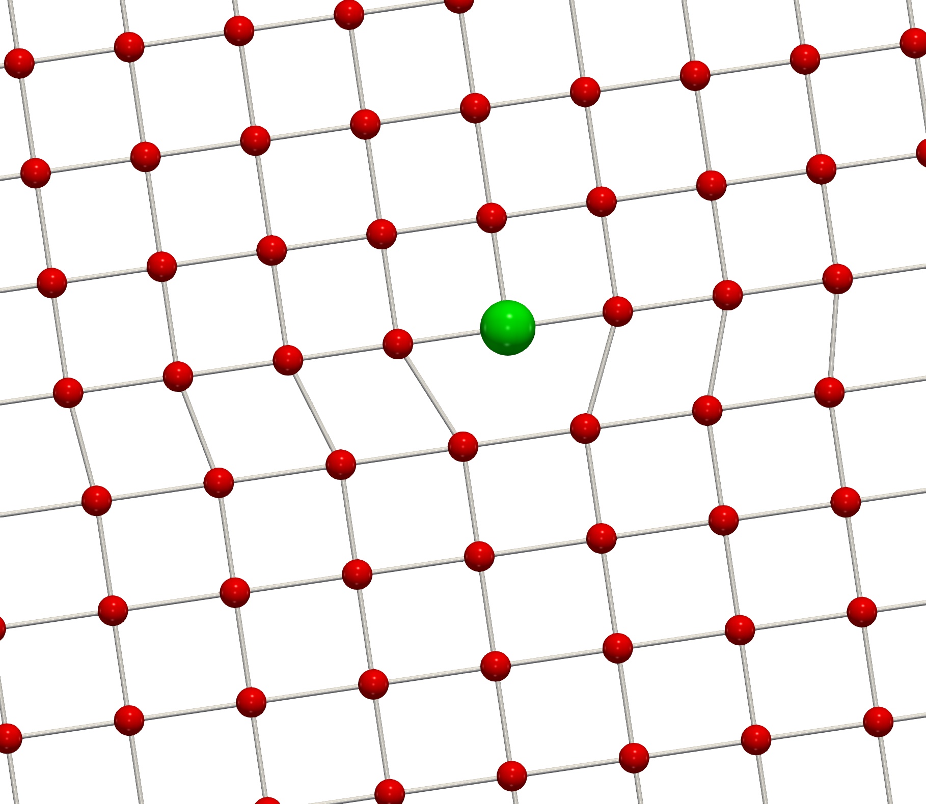
Figure 0.1: A topological defect in a crystal. One of the columns of atoms on bottom disappears halfway through the sample. The place where it disappears (highlighted in green) is a defect, because it doesn’t locally look like a piece of the perfect crystal.

The topological defects and their understanding are at the core of modern physics. The formalization of their properties, and of the knowledge of their role in a very broad range of physical processes is rather recent. However, they have been heuristically known by mankind for probably more than three thousand years. Indeed, this is approximately as far as the processes of quench hardening of metal by smiths can be traced back [2]. The fast thermal quenches used in metal hardening processes creates dislocations of the crystal structures, which are akin to topological defects. This is similar to the proliferation of topological defects that occur during phase transitions or other kinds of thermal quenches. As illustrated in Fig. 0.1, a dislocation in a crystal is a topological defect, because it cannot be removed by any local rearrangement.

Associated with broken symmetries, the topological defects are ubiquitous in physics. They indeed arise in a very broad context ranging from early universe cosmology and particle physics [3, 1, 4, 5, 6, 7, 8], to solid state and condensed matter systems [9, 10, 7]. Depending on the underlying theory, the topological defects can be of various kind including for example dislocation in crystals, monopoles, domain-walls, vortices, skyrmions, hopfions, and much more. They are intimately related with phase transitions [11, 12, 13], and their mere existence can have important consequences. For example, the possible formation of topological defects during early universe phase transitions could have greatly impacted the structure formation of the universe [5, 12, 14]. Likewise, they are believed to drive certain phase transitions in various physical system, as for example the vortex proliferation in superfluids and superconductors [11]. Vortices, which are line-like objects with specific topological properties, are probably the most studied topological defects.

Topological defects – Superconductors and superfluids

The vortex physics have been the subject of an intense scientific activity since the second half of the nineteenth century. Shortly after the earlier works of Helmholtz [15] on fluid dynamics, vortices were the cornerstone of the “vortex atom" theory of matter conjectured by Kelvin [16]. This failed attempt to classify the chemical elements as excitations consisting of closed, linked, and knotted vortex loops in the luminiferous aether , yet led to considerable breakthrough in topology as it motivated the creation of the first knot tables by Tait [17, 18, 19] and to the early knot theories works shortly after.

The theory of the vortex atom

Interestingly, the theory of the “vortex atom" of Kelvin and Tait still resonates with some concepts of modern physics [20, 21], and it inspired several works over the years. Hence, it is a story worth being told.

In his 1858 work on fluid dynamics, Helmholtz [15] demonstrated that in an ideal fluid (i.e. with an incompressible and inviscid flow), the circulation of a vortex filament does not vary over the time. He further demonstrated that a vortex cannot terminate inside such a fluid, but should either extend to the boundaries of the fluid or form closed loops. Also that, in the absence of external rotational forces, an initially irrotational flow remains irrotational.

Figure 0.2: A table of inequivalent knots.

Knowing the theorems of Helmholtz, in 1867 Kelvin [16] noticed that « (…) this discovery inevitably suggests the idea that Helmholtz’s rings are the only true atoms. » The general idea was that, because the vortex lines are frozen in the flow of an ideal fluid, then their topology should be invariant in time: «  It is to be remarked that two ring atoms linked together, or one knotted in any manner with its ends meeting, constitute a system which, however it may be altered in shape, can never deviate from its own peculiarity of multiple continuity (…)  ». That ideal fluid would be the luminiferous aether that people believed to fill the universe. He then attributed the spectroscopic properties of matter to the topology of such vortex lines: « It seems, therefore, probable that the sodium atom may not consist of a single vortex line; but it may very probably consist of two approximately equal vortex rings passing through one another, like two links of a chain. » . Kelvin further noticed that in models of « (…) knotted or knitted vortex atoms, the endless variety of which is infinitely more than sufficient to explain the varieties and allotropies of known simple bodies and their mutual affinities. ». In short Kelvin conjectured that the different chemical bodies consist in topologically inequivalent closed, linked and knotted vortex loops, illustrated in Fig. 0.2, of luminiferous aether.

Subsequently, Tait started to classify the different inequivalent ways to tie such knots [17, 18, 19]. These works pioneered the field of knots theory in algebraic topology. Kelvin’s theory was eventually falsified, when Michelson and Morley’s experiment ruled out the existence of aether [22]. Yet the paradigm to associate vortices in some underlying field with “elementary particles" re-emerged on several occasions. In a way, these knotted vortices can be seen as the first theoretical example of topological defects.

Vortices and other topological defects in modern physics

About 80 years after Kelvin’s work, it was realized by Onsager [23], and later formalized on solid theoretical grounds by Feynman [24], that the vortices occupy an important part in modern physics processes. In his work on superfluid ⁴He, Onsager [23] observed that the circulation of the superfluid velocity is quantized, and he further understood that vortex matter basically controls many of the key responses of superfluids. For example, that the superfluid to normal state phase transition is a thermal generation, and a proliferation of vortex loops and knots [23]. Also that vortices appear as the rotational response of superfluids.

These ideas somehow partially resonate with Kelvin’s theory of the vortex atom. Indeed, because the circulation of the superfluid velocity is quantized, then vortices in superfluids are topological defects. Moreover, the rotation of a superfluid results in the formation of a lattice or a liquid of these quantum vortices. These lattices could be seen as the vortex-matter realisation of crystals and liquids. It was also later predicted by Abrikosov [25] that the type-II superconductors should form magnetic vortices when subjected to an external magnetic field, by analogy with the vortices formed as a rotational response of a superfluid. Later it was further understood that in three dimensions superfluid and superconducting phase transitions are a thermal generation and a proliferation of vortex loops [26, 27].

Noteworthy, important progresses in modern physics phenomena, where vortices occupy a central part, were awarded a Nobel prize. As for example to Abrikosov in 2003 [28] for the understanding of their role in superconductors, or more recently in 2016 to Haldane, Kosterlitz and Thouless for their role in the phase transitions in two-dimensional systems [29, 11]. The concept of quantum vortices was later generalized to relativistic theories, as for example in the abelian-Higgs model [30]; theories that might have been relevant in the early universe [5, 31, 32], and also to the bosonic sector of the Weinberg-Salam theory of the electroweak interactions [33]. According to the Kibble-Zurek mechanism [12, 13], various kind of topological defects should be produced during possible early universe phase transitions. This would imply, among other things, that if topological defects were created, they could substantially contribute to the matter content of the universe, and have had a nontrivial impact on its history [5, 14]. These interesting ideas are at the origin of a lot interest for topological defects. This resulted in many seminal works and in a deeper understanding of the mathematical properties of topological defects.

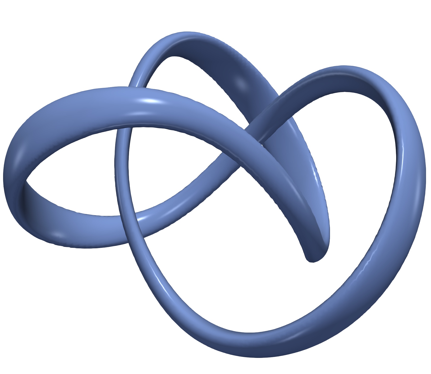
Figure 0.3: A trefoil knot in Skyrme-Faddev model.

Thus, as already emphasized there are plethora of different kind of topological defects, in a broad range of physical systems. It is kind of meaningless to exhaustively list all of them. Rather let’s mention two particular kinds of topological defects that particularly resonate with Kelvin’s theory, as they were somehow identified with states of matter. A first example is that of the topological defects in Skyrme model [34, 35]. The topological defects there are termed skyrmions , and the associated topological invariant is interpreted as the baryon number [36]. Likewise, the research on models supporting stable knotted topological defects has been of great interest in mathematics and physics, after the stability of these objects termed hopfions was demonstrated in the Skyrme-Faddeev model [37, 38, 39, 40, 41, 42] (for a review, see [43]). Hopfions in the Skyrme-Faddeev model resemble knots, as illustrated in Fig. 0.3.

After this general introduction about topological defects, most of the attention will be ported on vortices, with a particular focus on those that appear in models of superconductivity with multiple components of the order parameter.

Multi-component superconductors

Superconductivity and superfluidity are states of matter that are characterized by the macroscopic coherence of the underlying quantum excitations. The underlying physics that describes such systems are quantum fields theories, and these are the many-body properties, within those theories, that yield the macroscopic coherence of the quantum excitations. The very interesting feature is that such quantum many-body problems can be reduced, in the mean field approximation, to nonlinear classical field theories describing the macroscopic properties of the coherent state represented by a single complex scalar field (the order parameter). These mean field approximations are known as the Gross-Pitaevskii equations for superfluids, and as the Ginzburg-Landau equations for superconductors. Note that in the case of superconductors, the complex scalar is supplemented by a real Abelian vector field, describing the electromagnetic potential. This gauge field becomes massive via the Anderson-Higgs mechanism [44, 45], which is responsible for the Meissner effect [46]. While in the simplest textbook cases, these order parameters are singlets, they can be scalar multiplets in more complicated situations.

In condensed matter systems such as superfluids or Bose-Einstein condensates of ultra-cold atoms, theories with order parameters with multiple components (i.e. described by multiplets or even matrices of complex scalar fields) have been considered for a long time. They have been known to offer an extremely rich zoology of topological defects, as for example in superfluid helium [7, 47], spinor Bose-Einstein condensates [48, 49], or in neutron ${}^{3}P_{2}$ superfluids [50, 51]. In the context of superconductivity, theories with multiple superconducting gaps where considered from the earlier days of the Bardeen-Cooper-Schrieffer theory [52, 53, 54]. Yet these multiband/multicomponent theories where for a long time considered to describe exotic materials.

In the recent years however, there have been an increased interest in such materials, as the number of known multiband/multicomponent superconductor is rapidly growing. Indeed, in many superconductors, the pairing of electrons is supposed to occur on several sheets of a Fermi surface which is formed by the overlapping electronic bands. To name a few of them, this is for example the case of MgB₂ [55, 56], layer perovskite Sr₂RuO₄ [57, 58, 59], or of the familly of iron-based superconductors [60, 61, 62, 63]. Beyond solid state physics, multicomponent theories also apply to more exotic systems, as certain models of nuclear superconductors in the interior of neutron stars [64], or the superconducting state of Liquid Metallic Hydrogen [65, 66], Liquid Metallic Deuterium [67, 68] and other kind of metallic superfluids [69]. This opens the possibility of more complicated field theory models where, typically due to the existence of multiple broken symmetries, the physics of vortices (and of other topological defects) is extremely rich with no counterparts in single-component models.

Note that the models where vortices appear, in the context of high-energy physics, are typically very symmetric because of the underlying properties of the theory. For example, in the case of the Weinberg-Salam theory of the electroweak interactions, the theory is invariant (among other symmetries) under the local $\mathrm{SU}(2)$ rotations within the scalar doublet (the Higgs field). Models describing condensed matter systems are typically much less constrained on symmetry grounds, and thus allow for more interaction terms that explicitly break various symmetries. For example, in two-component superconductors (described by a scalar doublet) the global $\mathrm{SU}(2)$ invariance is explicitly broken down to a smaller subgroup (as for example $\mathrm{U}(1)\times\mathrm{U}(1)$). The absence of strong symmetry constraints, and thus the existence of various symmetry breaking terms is at the origin of many new features. It results, in particular, that vortices can acquire new properties and are associated to a broad range of new physical phenomena. Those new exotic properties can be understood as originating in the new broken symmetries. As a results such new phenomena can be used as signatures to trace back informations on the actual symmetries of some unknown state.

The crucial importance of the topological excitations in the physics of superconductivity made the Ginzburg-Landau vortices one of the most studied example of topological defects. Indeed, all the transport properties of superconductors crucially depend on the behaviour of magnetic vortices in these materials. For example, high critical currents in currently existing commercial superconducting transmission lines are only achieved by carefully controlling the vortex motion in these materials. The theories for multiband/multicomponent superconductors extends the usual Ginzburg-Landau theory by considering more than one superconducting order parameters. Because of the additional fields and the new broken symmetries, the spectrum of topological excitations and the associated signatures are much richer in multicomponent systems than in their single-component counterparts. For example multicomponent superconductors feature fractional vortices, singular/coreless vortices, skyrmions, hopfions, domain-walls, etc. All these topological excitations can be used as experimental signatures to probe the multicomponent nature of a superconducting system. Their observability can, for example, provide valuable informations about the structure of the order parameter and of the underlying pairing symmetry.

The works discussed in this report, deal with various aspects of the theories with more than one superconducting condensate. Both for general models of multicomponent superconductors and for material specific models. In particular through the investigation of the properties associated with the topological defects that appear therein.

Mean-field Ginzburg-Landau theories

In the single-component, weak-coupling, mean-field, Bardeen-Cooper-Schrieffer theory [70], the superconducting state is described by a classical complex field which is proportional to the gap function. Namely, the phenomenologically introduced Ginzburg-Landau theory [71] can be derived as the classical, mean-field, approximation of the microscopic theory [72], and the modulus of the order parameter is the density of Cooper pairs. There are various approaches to characterize the properties of superconducting materials, that are different/complementary to the Ginzburg-Landau theory. For example, methods such as the Bogoliubov-de Gennes formalism [73, 74], the Eilenberger [75] and Usadel [76] equations for transport, etc. However, the rest of this report is restricted only to the classical mean-field aspects of superconductivity of multicomponent systems. That is, to the multicomponent Ginzburg-Landau theory, and to the topological excitations that occur therein.

Interestingly, the Ginzburg-Landau theory of superconductivity attracted a lot of attention from the Numerical Analysts community only since the 1990s, after the report of the well-posedness of the problem [77, 78]. Since then, there have been quite some activity in understanding the mathematical properties of that problem, see for example [79, 80].

Field theoretical models in the mean field approximation

The details of the multicomponent models may vary, depending on the context of the underlying physical problem that is considered. For example, via the dependence of the different parameters. Here, we briefly expose the mathematical structure of the generic mean field models that describe multicomponent superconductors. The macroscopic properties of such physical systems are typically described by a Ginzburg-Landau (free) energy functional of the form:

$$\mathcal{F}/\mathcal{F}_{0}=\int_{\mathbb{R}^{3}}\frac{1}{2}\big{|}{\bm{\nabla}}\!\times\!{\bm{A}}\big{|}^{2}+\frac{\kappa_{ab}}{2}({\bm{D}}\psi_{a})^{*}{\bm{D}}\psi_{b}+\alpha_{ab}\psi_{a}^{*}\psi_{b}+\beta_{abcd}\psi_{a}^{*}\psi_{b}^{*}\psi_{c}\psi_{d}\,,$$ (1)

where $\psi_{a}$ are the components of the scalar multiplet $\Psi\in\mathbb{C}^{N}$, that accounts for the superconducting degrees of freedom. The scalar multiplet thus reads as $\Psi^{\dagger}=(\psi_{1}^{*},\psi_{2}^{*},\cdots,\psi_{N}^{*})$, where $a,b,c,d=1,\cdots,N$; and the repeated indices are implicitly summed over. The scalar fields are coupled to the (Abelian) gauge field ${\bm{A}}$ via the gauge derivative ${\bm{D}}={\bm{\nabla}}+ie{\bm{A}}$, with $e$ the gauge coupling (the bold fonts denote the vector quantities). All the matrix and tensor coefficients $\hat{\kappa}$, $\hat{\alpha}$, $\hat{\beta}$ obey some symmetry relations, so that the energy is a real positive definite quantity .

It might be convenient to collect all the potential terms in (1) into a single potential term $V(\Psi,\Psi^{\dagger})$ as

$$V(\Psi,\Psi^{\dagger})=\alpha_{ab}\psi_{a}^{*}\psi_{b}+\beta_{abcd}\psi_{a}^{*}\psi_{b}^{*}\psi_{c}\psi_{d}\,.$$ (2)

Sometimes, the specific structure of the potential $V(\Psi,\Psi^{\dagger})$ will be unimportant. On other occasions, the interacting potential will have a central role for the definition of the new physical properties. Thus the relevant restriction of the most generic potential (2) will be specified when necessary.

The ground state is the state which minimizes the potential energy (2) and that is constant in space: $\Psi_{0}:=\mathrm{argmin}\,V(\Psi,\Psi^{\dagger})$. Moreover the superconducting ground state is the state that minimizes the energy and that has $\Psi^{\dagger}\Psi=const.\neq 0$. The criterion for condensation, that is $\Psi_{0}\neq 0$, is that $\det\hat{\alpha}<0$. The superconducting ground state is degenerate in energy and this defines a manifold called the vacuum manifold. Roughly speaking this is the topology of that vacuum manifold that specifies the topological defects that can appear in the theory. For example, the ground state energy is invariant under overall phase rotations of the multiplet $\Psi$, thus this defines a vacuum manifold that is a circle. The field configurations are hence classified by a winding number that is an element of the first homotopy group $\pi_{1}(\mathbb{S}^{1})$ (this can alternatively be understood as a consequence that $\Psi$ has to be single-valued). This winding number determines the vortex content of the theory.

The functional variation of the free energy with respect to the superconducting condensates yields the Euler-Lagrange equations of motion. These, in the framework of superconductivity, are the Ginzburg-Landau equations

$$\kappa_{ab}{\bm{D}}{\bm{D}}\psi_{b}=2\frac{\delta V}{\delta\psi_{a}^{*}}\,.$$ (3)

Similarly, the variation with respect to the gauge field yields the Ampère-Maxwell equation

$${\bm{\nabla}}\!\times\!{\bm{B}}+e\sum_{a,b}\kappa_{ab}\mathrm{Im}\big{(}\psi_{a}^{*}{\bm{D}}\psi_{b}\big{)}=0\,,$$ (4)

where ${\bm{B}}={\bm{\nabla}}\!\times\!{\bm{A}}$ is the magnetic field. This equation is used to introduce the supercurrents

$${\bm{J}}:=\sum_{a}{\bm{J}}^{(a)}\,,\leavevmode\nobreak\ \leavevmode\nobreak\ \leavevmode\nobreak\ \leavevmode\nobreak\ \leavevmode\nobreak\ \text{where}\leavevmode\nobreak\ \leavevmode\nobreak\ \leavevmode\nobreak\ \leavevmode\nobreak\ \leavevmode\nobreak\ {\bm{J}}^{(a)}=e\sum_{b}\kappa_{ab}\mathrm{Im}\big{(}\psi_{a}^{*}{\bm{D}}\psi_{b}\big{)}\,.$$ (5)

Here ${\bm{J}}$ is the total supercurrent, while ${\bm{J}}^{(a)}$ is the partial current associated with a given superconducting condensate $\psi_{a}$.

Depending on the properties of the microscopic model under consideration, there can be various additional requirements further constraining the structure of the tensor parameters $\hat{\kappa}$, $\hat{\alpha}$, $\hat{\beta}$. This can yield many different situations that are useless to be listed here. As mentioned above, the vortex content is specified by the winding number of the field configuration (more precisely the winding at infinity). The next step is to explicitly construct the vortex solutions in a given topological sector specified by this winding number. The theory is clearly nonlinear and the explicit construction of a field configuration with a given winding number thus has to be addressed numerically. In the works that are discussed here, this is done using minimization algorithms on the energy within a finite element formulation of the problem (see details in the Appendix B).

Outline

It is hardly conceivable to disentangle all the aspects related to the new physics that appear in multicomponent systems. Hence there will surely be some kind of an overlap from time to time. Anyway, the main body of this report is organized as follows: First, the Chapter 1 sheds the light on the new properties associated with the topology of the phenomenological multicomponent models. Next, Chapter 2 presents some new physical properties that occur because of the existence of additional length scales. Finally, the properties of multicomponent superconducting states that spontaneously break the time-reversal symmetry are discussed in the Chapter 3.

More precisely, the Chapter 1 is focused on the nature of the topological excitations that appear in multicomponent superconductors. It is first demonstrated that the condition for the quantization of the magnetic flux implies that the elementary topological excitations there, are fractional vortices. These are field configurations that carry an arbitrary fraction of the flux quantum, but that have a divergent energy per unit length. Yet when the fractional vortices combine to form an object that carries an integer amount of flux, they form a topological defect which has a finite energy. Depending on the relative position of the ensuing fractional vortices, the resulting topological defect is either singular or coreless. In the later case, it can then be demonstrated that there exists an additional topological invariant of a different nature than the most common winding number. However, the most simple analysis shows that typically the fractional vortices attract each other to form a singular defect. It follows that a stabilizing mechanism is necessary for the existence of coreless defects. Various occurrence of such stable coreless topological defects, termed skyrmions, are discussed along that chapter. As they have a different core structure, the skyrmions, can interact differently than the singular (Abrikosov) vortices, and thus have significantly different observable properties.

While the coreless defects feature interesting new properties, the singular defects also exhibit a rich new physics. This new physics of the singular defects is discussed in the Chapter 2. The properties of the magnetic response of superconductors can, to some extent, be seen as the consequence of the interaction between vortices. More precisely, the textbook dichotomy that classifies the conventional superconductors into type-1 or type-2 can be understood by whether the vortices attract or if they repel. The vortex interactions can be determined by the analysis of the length-scales of the theory. Vortices attract when the coherence length is larger than the penetration depth of the magnetic field (this is the type-1 regime). On the other hand, if the penetration depth is the largest length scale, vortices repel each other (this is the type-2 regime). In multicomponent superconductors such a dichotomy is not always possible. Indeed, because they have several superconducting condensates, the multicomponent superconductors usually feature additional length scales. It thus can happen that the penetration depth is an intermediate length scale, and that the vortex interaction is long-range attractive (as in type-1) and short-range repulsive (as in type-2). Such a regime with non-monotonic intervortex forces is termed type-1.5. In that regime vortices tend to aggregate to form large clusters surrounded by vortex-less regions of the Meissner state. The possible formation of such aggregates strongly impact the magnetization properties, as compared to the conventional type-1 or type-2 regimes.

The non-monotonic interactions between vortices are (partially) determined by the length-scales, and these are determined by the perturbations of the theory around the ground state. As discussed in the Chapter 3, certain multicomponent superconductors feature unusual ground states that spontaneously break the time-reversal symmetry. These states are characterized by ground state relative phases between the condensates that are neither 0 nor $\pi$. Depending on the pairing symmetries, there exists various such superconducting states, e.g. termed ${p\!+\!ip}$, ${s\!+\!is}$, ${s\!+\!id}$, ${d\!+\!id}$, etc. Yet, the focus will mostly be about ${s\!+\!is}$ state, which the simplest extension of the most abundant $s$-wave state, that break the time-reversal symmetry. The spontaneous breakdown of the time-reversal symmetry in the ${s\!+\!is}$ state typically occurs as a consequence of the competition between different phase-locking terms. The phase transition to the time-reversal symmetry broken states is of the second order, so it is associated with a divergent length scale. Notably this transition can occur within the superconducting state, where the penetration depth is finite. It follows that, in the vicinity of the time-reversal symmetry breaking transition, the penetration depth can be an intermediate length scale, thus leading to the non-monotonic vortex interactions mentioned above. Moreover, the time-reversal symmetry is a discrete operation, so if it is spontaneously broken, then the ground state has a discrete $\mathbb{Z}_{2}$ degeneracy in addition to the usual $\mathrm{U}(1)$. This implies that, in addition to the vortices, the theory allows for domain-walls excitations. They interact non-trivially with the vortex matter, and this results in a new kind of topological excitations with different magnetization properties. Finally, the superconducting states that break the time-reversal symmetry also feature unusual thermoelectric properties. These can be used to induce specific electric and magnetic responses, when exposed to an inhomogeneous local heating.

As explain above, the essential of these effects that appear in multicomponent superconductors, are discussed here in the framework of the Ginzburg-Landau theory. The Appendix A, presents the theoretical framework, and the textbook properties of the single-component Ginzburg-Landau theory. It indeed might be useful, for example in order to compare with the properties of the multicomponent Ginzburg-Landau theories. This may provide a better insight to understand the new features of the multicomponent theories.

It is emphasized on several occasions that the Ginzburg-Landau theory is a nonlinear classical field theory. Being nonlinear implies that except under very special circumstances there are no analytic solutions, and the problem has to be addressed numerically. This is in particular the case of the results displayed in this work, and of the results that are discussed there. Technical aspects of the numerical methods are discussed in the Appendix B. This includes a presentation of the finite element methods used to handle the spatial discretization of the partial differential equations; also the optimization algorithm to handle the nonlinear problem. The numerical construction of topological defects also relies on the appropriate implementation of the topological properties for the numerical algorithm; this is also discussed there.

Remark:

The next chapters will follow the plan presented above. They are written, so that they are as self-contained as possible. Yet there will occasionally be some overlap. There will also be some redundancy, in particular with the general introduction, when developing the introduction part within each chapter.

Chapter 1 Topological defects in multicomponent systems

Unlike single-component Ginzburg-Landau theory, where the topological excitations merely consists in quantum vortices, theories with multicomponent order parameters feature a much richer spectrum of topological excitations. Multicomponent superconductors and superfluids, are described by order parameters for which each of the component is commonly described by a complex field. Overall, all the superconducting/superfluid degrees of freedom can be cast into a multiplet of complex scalar fields.

The following chapter presents results concerning the properties of the topological excitations in theories of superconductivity featuring multiple order parameters or order parameters with multiple components. In the context of superconductivity, theories with multiple superconducting gaps where considered from the earlier days of the Bardeen-Cooper-Schrieffer theory [52, 53, 54]. Yet these multicomponent/multiband theories where for a long time considered to describe exotic materials. In the recent years however, there have been an increased interest in such materials, as the number of known multicomponent superconductor have been rapidly growing. For example materials such as Sr₂RuO₄ [57, 58], MgB₂ [55], heavy fermion compounds such as UPt₃ [81], the family of iron based superconductors [60], are understood to be multicomponent/multiband.

The topological properties of multicomponent systems have been widely investigated in the context of superfluid ³He, see e.g. [82, 83], and the detailed books [47, 7]. Superfluid ³He has been particularly known to host a broad variety of unusual topological defects [84, 85, 86, 87, 88]. More recently, in the context ultracold atomic gases, the topological properties of spinor Bose-Einstein condensates were also investigated in great details [89, 90, 48, 49]. This chapter presents the topological properties of phenomenological, multicomponent, Ginzburg-Landau models of superconductivity. An overview of the properties of the conventional, single-component, Ginzburg-Landau models of superconductivity is given in the Appendix A. This might indeed be useful for the comparison with the new properties that appear in multicomponent systems.

In the context of multicomponent superconductors and superfluids, the most elementary topological excitations are fractional vortices. For superfluids, these objects carry a fraction of the circulation of the superfluid velocity, while for superconductors they carry a fraction of the flux quantum [91, 92, 93]. In short, a fractional vortex is a field configuration of a multicomponent system for which only a single component has a nonzero phase winding.

In some specific models of superconductivity, the fraction carried by the fractional vortices is half of a flux quantum (or half of a circulation quantum, in the case of superfluids). There, the fractional vortices are rather termed half-quantum vortices. Half-quantum vortices were originally predicted to exist in $A$-phase of superfluid ³He [94, 95]. Their existence was relentlessly investigated for, and their observation was eventually reported in the polar phase of superfluid ³He [96].

The search for half-quantum vortices, have also been very active in solid state physics. In particular for superconductors which have been argued to have a $p$-wave pairing, such as Sr₂RuO₄ [97, 98, 99]. The observation of half of a flux quantum steps, in the magnetization curves of mesoscopic Sr₂RuO₄ samples, was claimed to be the hallmark of half-quantum vortices [100]. The interest in the realization of half-quantum vortices follows from that their excitation spectrum contains zero-energy Majorana fermions [101]. It follows that the statistics of vortices is non-Abelian [101], which could potentially be used for quantum computations [102].

As discussed below, the fractional vortices in multicomponent superconductors do not have a finite energy (per unit length) and the only finite energy topological excitations carry an integer amount of the flux quantum. It follows that, under usual conditions, fractional vortices are thermodynamically unstable in bulk systems. Note however that complex setups, such as mesoscopic samples, can allow for fractional vortices to be energetically favoured [103, 104]. Despite the non-finiteness of their energy, the fractional vortices are crucially important for multicomponent superconductors. Indeed, they can form bound states that carry an integer amount of the flux quantum, for which the divergences of the energy compensate.

Hence, fractional vortices are quite elusive objects that, in general, cannot be observed individually. Yet their integer flux bound states have finite energy, and thus are observable . Such integer flux carrying bound states are termed composite vortices. There are basically two qualitatively different possibilities to form integer flux composite objects. The first is to superimpose the singularities of all constituting fractional vortices, and the resulting objects are thus singular composite vortices. The other possibility is to form a bound state for which the individual singularities do not overlap. The ensuing objects are thus coreless topological defects. As detailed in this chapter, these feature additional topological invariants, that can discriminate them from singular defects. Because of these additional topological properties, these coreless defects are often termed skyrmions.

Fractional vortices are not only important as they are the building blocks of more complex topological excitations, they are also the cornerstone of the thermodynamical properties of multicomponent systems. In single-component superconductors, the superconducting phase transition was demonstrated to be driven by the proliferation of thermally excited vortex loops [26, 27]. Likewise, in multicomponent superconductors, this is the proliferation of fractional vortices that drives the superconducting phase transitions, as demonstrated for London superconductors [105, 106, 107], or in Ginzburg-Landau [108]. In the presence of an external field, fractional vortices also play a role in the melting of vortex lattices [108]. Similarly the thermodynamic properties of multicomponent superfluids strongly depend on the role of fractional vortices [109, 110, 111].

This chapter, about the topological properties of multicomponent superconductors thus heavily relies on the concept of fractional vortices. They are indeed crucial in our understanding of the responses of the multicomponent systems. Below is a plan that details the structure of this chapter, followed by a brief summary of the author’s contributions about these topological properties.

Plan of the Chapter

As a starting point, the Section 1.1 addresses the question of the flux quantization in multicomponent superconductors. It is shown there, that the flux quantization formally allows the existence of fractional vortices. Their basic properties are also discussed. In multicomponent systems, the fractional vortices are field configurations, where only a single condensate has a phase winding, while the others do not. The energy of individual fractional vortices is divergent. However, as already emphasized, the energetic divergence of fractional vortices disappears if they form bound states.

This implies that, in bulk systems, only composite objects have finite energy. The Section 1.1.3 further develops on the topological properties of the composite topological defects for multicomponent superconductors. In particular, there exist a hidden topological invariant associated with the topology of the complex projective space, that characterizes coreless topological defects. This invariant, that classifies the maps $\mathbbm{R}^{2}\to\mathbb{C}\mathrm{P}^{N-1}$, discriminates coreless from singular vortices. In the case of a two-component system, the target $\mathbb{C}\mathrm{P}^{1}$ space can be identified with the unit two-sphere $\mathbb{S}^{2}$. The topological invariant can thus be interpreted as the Hopf index, and can be used to characterize knotted vortices in two-component superconductors.

The flux quantization implies that these additional invariant are non-zero, as long as not all of the superconducting condensates simultaneously vanish. That is, as long as the fractional vortices in the different components do not overlap. The interaction between fractional vortices is discussed in Section 1.1.4. Because the interaction between fractional vortices is attractive, the observation of coreless topological defects is rather difficult. As explained later on, various mechanisms can compensate the attraction between fractional vortices and thus lead the formation of coreless defects. These coreless defects that consist in a bound state of fractional vortices are often termed skyrmions. This terminology originates in the existence of a formal relation between the two-component Ginzburg-Landau models and the Skyrme-Faddeev model. The relation between these two models is explained in Section 1.2.

The Section 1.3 presents various situations, origintating in different physical mechanisms, that allow the stabilization of coreless defects rather than singular vortices. First, in Section 1.3.1, in a model of mixtures of condensates with commensurate charges, introduced in [JG18.]. In this rather exotic model, the different superconducting condensates can feature different electric charges (i.e. different coupling to the gauge field). There, fractional vortices are naturally split, and thus form coreless bound states. This model can be applied to describe the superconducting state for liquid metallic deuterium, where the electronic Cooper pairs coexist with a Bose-Einstein condensate of deuterons.

Next, in Section 1.3.2, the dissipationless intercomponent drag, known as the Andreev-Bashkin effect, is demonstrated to be responsible for the existence of skyrmions [JG20.]. Furthermore, the dissipationless drag can also stabilize knotted bound states of fractional vortices [JG4.]. These knots, characterized by the Hopf index, are hence termed hopfions. Interestingly, these hopfions remind Kelvin’s earlier idea of knotted vortices of luminiferous aether to explain classification of atoms.

Next, the properties of topological defects that occur in superconducting ${s\!+\!is}$ states are discussed in Section 1.3.3. As discussed in more details in Chapter 3, these ${s\!+\!is}$ states break a discrete $\mathbb{Z}_{2}$ symmetry associated with the time-reversal symmetry, in addition to the usual $\mathrm{U}(1)$ gauge symmetry. The spontaneous breakdown of a discrete symmetry is associated with formation of domain walls. Following [JG19.] these domain walls can be formed by thermal quench, and geometrically stabilized against collapse. As demonstrated in [JG26.] and [JG21.], the complex interaction between domain-walls and fractional vortices leads to the existence of new skyrmionic states.

Summary of the results that are discussed in this chapter

• In [JG23.] and [JG13.], we showed that the $p_{x}\!+ip_{y}$ superconducting state allows for skyrmionic excitations characterized by the homotopy invariants of the $\mathbb{S}^{2}\!\to\!\mathbb{S}^{2}$ maps. They can be alternatively understood as vortices carrying two quanta of the magnetic flux, that are energetically favoured as compared to single-quanta vortices [JG13.]. These two-quanta vortices form hexagonal lattices in an external field [JG11.]. Close to $H_{c2}$ the hexagonal lattices of two-quanta vortices dissociate into square lattices of single quantum vortices [JG11.], and this picture persists beyond the mean field approximation [JG3.].

• Demonstration of an unconventional magnetic response in interface superconductors with a strong Rashba spin-orbit coupling [JG17.]. In the clean limit, interface superconductors, such as SrTiO₃/LaAlO₃, are ideal candidates to observe coreless defects characterized by homotopy invariants of $\mathbb{S}^{2}\to\mathbb{S}^{2}$ maps, in addition to those of $\mathbb{S}^{1}\to\mathbb{S}^{1}$ maps. Similar skyrmionic states also exist in parity-odd nematic superconductors [JG7.].

• Identification of the topological properties of flux-carrying topological defects in mixtures of charged condensates that have different (commensurate) electric charges [JG18.]. Such situation is expected to appear for example in liquid metallic deuterium.

• Prediction of a new phase in $\mathrm{U}(1)\!\times\!\mathrm{U}(1)$ superconductors with interspecies dissipationless drag [JG20.]. The dissipationless current interaction renders vortices unstable in favour of skyrmions whose long-range interaction substantially modifies magnetization processes. These models of superconductivity with disspationless drag support stable knotted vortices [JG4.]. These knots share many properties with the knots in luminiferous aether conjectured by Kelvin.

• Discovery of new kind of stable topological solitons in three-component superconductors with spontaneously broken time-reversal symmetry [JG26.], and [JG21.]. These flux carrying topological defects, characterized by $\mathbb{C}\mathrm{P}^{2}$ topological invariants are skyrmions. Their observation could signal superconducting states that break the time-reversal symmetry, for example in some iron based superconductors, as well as in Josephson-coupled bilayers of $s_{\pm}$ and ordinary $s$-wave superconductor.

1.1 Flux quantization and fractional vortices

In multicomponent superconductors, the flux quantization relation is modified compared to that of single-component superconductors (see the background discussion in Section A.3). This modified relation implies the existence of vortices that carry arbitrary fractions of the elementary flux quantum $\Phi_{0}$, without violating the flux quantization itself. To illustrate this feature of multicomponent systems, let consider here a restriction of the generic free energy (1), in the absence of mixed gradient terms. Namely, the gradient coupling matrix $\kappa_{ab}$ is the identity $\kappa_{ab}=\delta_{ab}$, and the Ginzburg-Landau free energy reads as

$$\mathcal{F}/\mathcal{F}_{0}=\bigintsss\frac{1}{2}\big{|}{\bm{\nabla}}\!\times\!{\bm{A}}\big{|}^{2}+\sum_{a}\frac{1}{2}\big{|}{\bm{D}}\psi_{a}\big{|}^{2}+V(\Psi,\Psi^{\dagger})\,.$$ (1.1)

Here again, $\psi_{a}=|\psi_{a}|e^{i\varphi_{a}}$ are complex fields representing the superconducting condensates, labelled by the index $a=1,2,\cdots,N$. For the moment, the specific structure of the potential $V(\Psi,\Psi^{\dagger})$ is rather unimportant. The potential will be specified later when it is necessary. Again, besides the potential term, the condensates are indirectly coupled by the electromagnetic interaction via the gauge derivative in the kinetic term ${\bm{D}}={\bm{\nabla}}+ie{\bm{A}}$. The Ampère-Maxwell equation (4) now reads as

$${\bm{\nabla}}\!\times\!{\bm{B}}+{\bm{J}}=0\,,$$ (1.2)

where the supercurrent is

$${\bm{J}}\equiv e\sum_{a}|\psi_{a}|^{2}\big{(}{\bm{\nabla}}\varphi_{a}+e{\bm{A}}\big{)}=e^{2}\varrho^{2}{\bm{A}}+e\sum_{a}|\psi_{a}|^{2}{\bm{\nabla}}\varphi_{a}\,,\leavevmode\nobreak\ \leavevmode\nobreak\ \leavevmode\nobreak\ \text{with}\leavevmode\nobreak\ \leavevmode\nobreak\ \varrho^{2}=\sum_{a}|\psi_{a}|^{2}\,,$$ (1.3)

here $\varrho^{2}$ is the total superconducting density. Here again, the total superconducting current ${\bm{J}}$ can be decomposed in terms of the contributions of the partial currents ${\bm{J}}^{(a)}$ carried by the individual condensate $\psi_{a}$, as

$${\bm{J}}=\sum_{a}{\bm{J}}^{(a)}\,,\leavevmode\nobreak\ \leavevmode\nobreak\ \leavevmode\nobreak\ \leavevmode\nobreak\ \leavevmode\nobreak\ \text{with}\leavevmode\nobreak\ \leavevmode\nobreak\ \leavevmode\nobreak\ \leavevmode\nobreak\ {\bm{J}}^{(a)}=e|\psi_{a}|^{2}\big{(}{\bm{\nabla}}\varphi_{a}+e{\bm{A}}\big{)}\,.$$ (1.4)

1.1.1 Separation in charged and neutral modes

To understand the role of the fundamental excitations (i.e. fractional vortices), the Ginzburg-Landau free energy (1.1) can be rewritten into charged and neutral modes, by expanding the kinetic term as

$$\sum_{a}\big{|}{\bm{D}}\psi_{a}\big{|}^{2} =\sum_{a}\big{(}{\bm{\nabla}}|\psi_{a}|\big{)}^{2}+\sum_{a}|\psi_{a}|^{2}\big{(}{\bm{\nabla}}\varphi_{a}+e{\bm{A}})^{2}$$ (1.5)

$$=\sum_{a}\big{(}{\bm{\nabla}}|\psi_{a}|\big{)}^{2}+\sum_{a}|\psi_{a}|^{2}\big{(}{\bm{\nabla}}\varphi_{a})^{2}+{\bm{A}}\cdot\Big{(}e^{2}{\bm{A}}\sum_{a}|\psi_{a}|^{2}+2e\sum_{a}|\psi_{a}|^{2}{\bm{\nabla}}\varphi_{a}\Big{)}\,.$$ (1.6)

Now, using the definition of the current (1.3), allows to eliminate the vector potential, and the kinetic term thus reads as:

$$\sum_{a}\big{|}{\bm{D}}\psi_{a}\big{|}^{2} =\sum_{a}\big{(}{\bm{\nabla}}|\psi_{a}|\big{)}^{2}+\sum_{a}|\psi_{a}|^{2}\big{(}{\bm{\nabla}}\varphi_{a})^{2}$$ (1.7)

$$+\frac{1}{e^{2}\varrho^{2}}\Big{(}{\bm{J}}-e\sum_{a}|\psi_{a}|^{2}{\bm{\nabla}}\varphi_{a}\Big{)}\cdot\Big{(}{\bm{J}}+e\sum_{a}|\psi_{a}|^{2}{\bm{\nabla}}\varphi_{a}\Big{)}$$ (1.8)

$$=\sum_{a}\big{(}{\bm{\nabla}}|\psi_{a}|\big{)}^{2}+\sum_{a}|\psi_{a}|^{2}\big{(}{\bm{\nabla}}\varphi_{a})^{2}+\frac{{\bm{J}}^{2}}{e^{2}\varrho^{2}}-\frac{\big{(}\sum_{a}|\psi_{a}|^{2}{\bm{\nabla}}\varphi_{a}\big{)}^{2}}{\varrho^{2}}$$ (1.9)

$$=\sum_{a}\big{(}{\bm{\nabla}}|\psi_{a}|\big{)}^{2}+\frac{{\bm{J}}^{2}}{e^{2}\varrho^{2}}+\frac{1}{\varrho^{2}}\sum_{a,b}|\psi_{a}|^{2}|\psi_{b}|^{2}{\bm{\nabla}}\varphi_{a}\cdot({\bm{\nabla}}\varphi_{a}-{\bm{\nabla}}\varphi_{b})$$ (1.10)

$$=\sum_{a}\big{(}{\bm{\nabla}}|\psi_{a}|\big{)}^{2}+\frac{{\bm{J}}^{2}}{e^{2}\varrho^{2}}+\sum_{a,b>a}\frac{|\psi_{a}|^{2}|\psi_{b}|^{2}}{\varrho^{2}}({\bm{\nabla}}\varphi_{a}-{\bm{\nabla}}\varphi_{b})^{2}\,.$$ (1.11)

Hence the kinetic energy can be expressed in terms of three contributions: the density term, the charged mode that involves the current ${\bm{J}}$, and the neutral mode which involves only the relative phase $\varphi_{ab}:=\varphi_{b}-\varphi_{a}$ between condensates. The free energy now can be written as

$$\mathcal{F}/\mathcal{F}_{0}=\bigintsss\frac{{\bm{B}}^{2}}{2}+\sum_{a}\frac{1}{2}\big{(}{\bm{\nabla}}|\psi_{a}|\big{)}^{2}+\frac{{\bm{J}}^{2}}{2e^{2}\varrho^{2}}+\sum_{a,b>a}\frac{|\psi_{a}|^{2}|\psi_{b}|^{2}}{2\varrho^{2}}({\bm{\nabla}}\varphi_{ab})^{2}+V(\Psi,\Psi^{\dagger})\,.$$ (1.12)

1.1.2 Factional vortices

The existence of vortices carrying an arbitrary fraction of the flux quantum follows from the evaluation of the flux for a multicomponent superconductors. The Stokes’ theorem implies that the flux of the magnetic field through a given area ${\cal A}$ can be expressed as the line integral over the contour ${\cal C}$ which bounds that area $\Phi=\int_{\cal A}{\bm{B}}\!\cdot\!d{\bm{S}}=\oint_{\cal C}{\bm{A}}\!\cdot\!d{\bm{\ell}}$. Given the definition of the current (1.3), the vector potential can be expressed in term of the current ${\bm{J}}$ and of the individual phase gradients ${\bm{\nabla}}\varphi_{a}$. Hence, the magnetic flux reads as

$$\Phi=\frac{1}{e^{2}\varrho^{2}}\bigointsss_{\!\!\!\!\!\!{\cal C}}\left({\bm{J}}-e\sum_{a}|\psi_{a}|^{2}{\bm{\nabla}}\varphi_{a}\right)\!\cdot\!d{\bm{\ell}}\,.$$ (1.13)

Given a large contour ${\cal C}$, finite energy considerations imply that the total current ${\bm{J}}$ vanishes on that contour (Meissner screening implies that the current is exponentially suppressed), and that the individual densities $|\psi_{a}|$ are constant to their ground state value. Indeed, the spontaneous breakdown of the $\mathrm{U}(1)$ symmetry implies that the vector potential ${\bm{A}}$ is massive, and so is the current ${\bm{J}}$ (i.e. the Meissner effect). The first term in (1.13) thus vanishes, and the flux reads as

$$\Phi=\frac{-1}{e\varrho^{2}}\bigointsss_{\!\!\!\!\!\!{\cal C}}\sum_{a}|\psi_{a}|^{2}{\bm{\nabla}}\varphi_{a}\!\cdot\!d{\bm{\ell}}=\frac{\Phi_{0}\sum_{a}|\psi_{a}|^{2}}{2\pi\varrho^{2}}\bigointsss_{\!\!\!\!\!\!{\cal C}}{\bm{\nabla}}\varphi_{a}\!\cdot\!d{\bm{\ell}}\,,$$ (1.14)

where $\Phi_{0}=2\pi/e$ is the flux quantum .

Each of the condensate has to be single valued, hence the phase of the complex fields $\varphi_{a}$ winds only an integer number of times $n_{a}$ and thus $\oint_{\cal C}{\bm{\nabla}}\varphi_{a}\!\cdot d{\bm{\ell}}=2\pi n_{a}$. The individual winding number $n_{a}$ of a condensate is independent of the winding of the other condensates. It thus makes sense to consider the possibility where only a single condensate, say $\psi_{a}$ has a unit winding: $\oint_{\cal C}{\bm{\nabla}}\varphi_{a}\!\cdot d{\bm{\ell}}=2\pi$, while all the other condensates have zero winding: $\oint_{\cal C}{\bm{\nabla}}\varphi_{b}\!\cdot d{\bm{\ell}}=0$ (for $b\neq a$). It results that the configuration for which only one of the condensates has a nonzero winding, carries the flux $\Phi_{a}=\Phi_{0}|\psi_{a}|^{2}/\varrho^{2}$. Such a configuration thus carries only a fraction $|\psi_{a}|^{2}/\varrho^{2}$, of the elementary flux quantum $\Phi_{0}$. Conversely, if all components have the same winding number ($n_{1}=n_{2}=\cdots\equiv n$), then the flux is quantized: $\Phi=n\Phi_{0}$.

The configurations, with a winding in only a single condensate, and that hence carry only a fraction the elementary flux quantum $\Phi_{0}$ are called fractional vortices [91]. As earlier mentioned, these objects occupy a central place in the statistical properties of multicomponent superfluids [112, 111, 109, 110, 107] and of multicomponent superconductors [113, 114, 106, 108, 105, 93].

Note however that the existence of vortex excitations carrying only a fraction of the flux quantum, does not contradict the traditional arguments for the quantization of the magnetic flux. Indeed when considering straight vortex lines, it turns out that fractional vortices have an infinite energy per unit length. This follows from that a single fractional vortex induces a nonzero winding of the relative phases in the neutral modes of (1.12). Thus straight fractional vortices have logarithmically divergent energy. Indeed, consider for example the simplest case where only $n_{1}=1$ and $n_{b}=0$ ($b\neq 1$). Then the part of the free energy containing gradients of the relative phase is

$$\cdots+\sum_{b\neq 1}\frac{|\psi_{1}|^{2}|\psi_{b}|^{2}}{2\varrho^{2}}({\bm{\nabla}}\varphi_{1b})^{2}+\cdots\,.$$ (1.15)

At a large distance $r$ from the core, the densities are approximately constant and thus the contribution of the neutral sector is approximated by

$$\sim\int_{r_{0}}^{r}r^{\prime}dr^{\prime}\left(\frac{1}{r^{\prime}}\partial_{\theta}\varphi_{1b}\right)^{2}\sim\int_{r_{0}}^{r}\frac{dr^{\prime}}{r^{\prime}}\sim\log\frac{r}{r_{0}}\,,$$ (1.16)

Where $r$ and $\theta$ are respectively the radius, and the polar angle of cylindrical coordinates. Note that if $V(\Psi^{\dagger},\Psi)$ features phase-locking terms (i.e. potential terms involving the relative phase $\varphi_{ab}$, like the Josephson coupling), then the logarithmic divergence of the energy becomes linear. This is for example discussed in details, in the appendix of [JG21.]. In any case, the divergence due to the winding in the relative phase puts a strong energy penalty on the existence of fractional vortices.

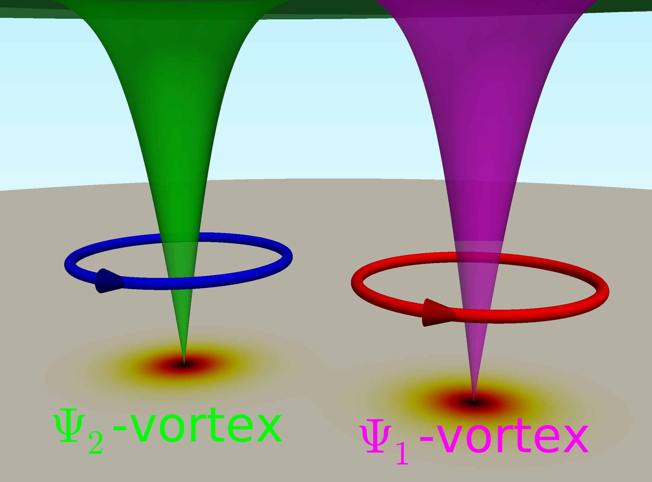
Figure 1.1: Schematic illustration of a composite vortex, in the case of a two-component system. The cones show the densities $|\psi_{a}|$ that vanish at the vortex core. The closed arrows denote the phase winding, and the circulation of the supercurrents.

On the other hand, if all condensates have the same winding number, then there is no winding of the relative phases. As a results, the long-range contribution of the neutral modes vanishes, and the corresponding energy is finite. Thus, the only configurations that yield a finite energy per unit length are those where all condensates have the same winding, and hence carry an integer flux. As a result, the configurations with a fractional flux cannot be excited in bulk superconductors. Note however that they can be stabilized near boundaries [104, 115], in mesoscopic samples [91, 116, 117, 103, 118] or in samples with geometrically trapped domain walls [119]. In bulk systems, the condition for the finiteness of the energy, thus allows only topological defects that carry integer flux quanta. These objects, made of fractional vortices in each of the components, are thus composite objects. Such a composite vortex is sketched in Fig. 1.1.

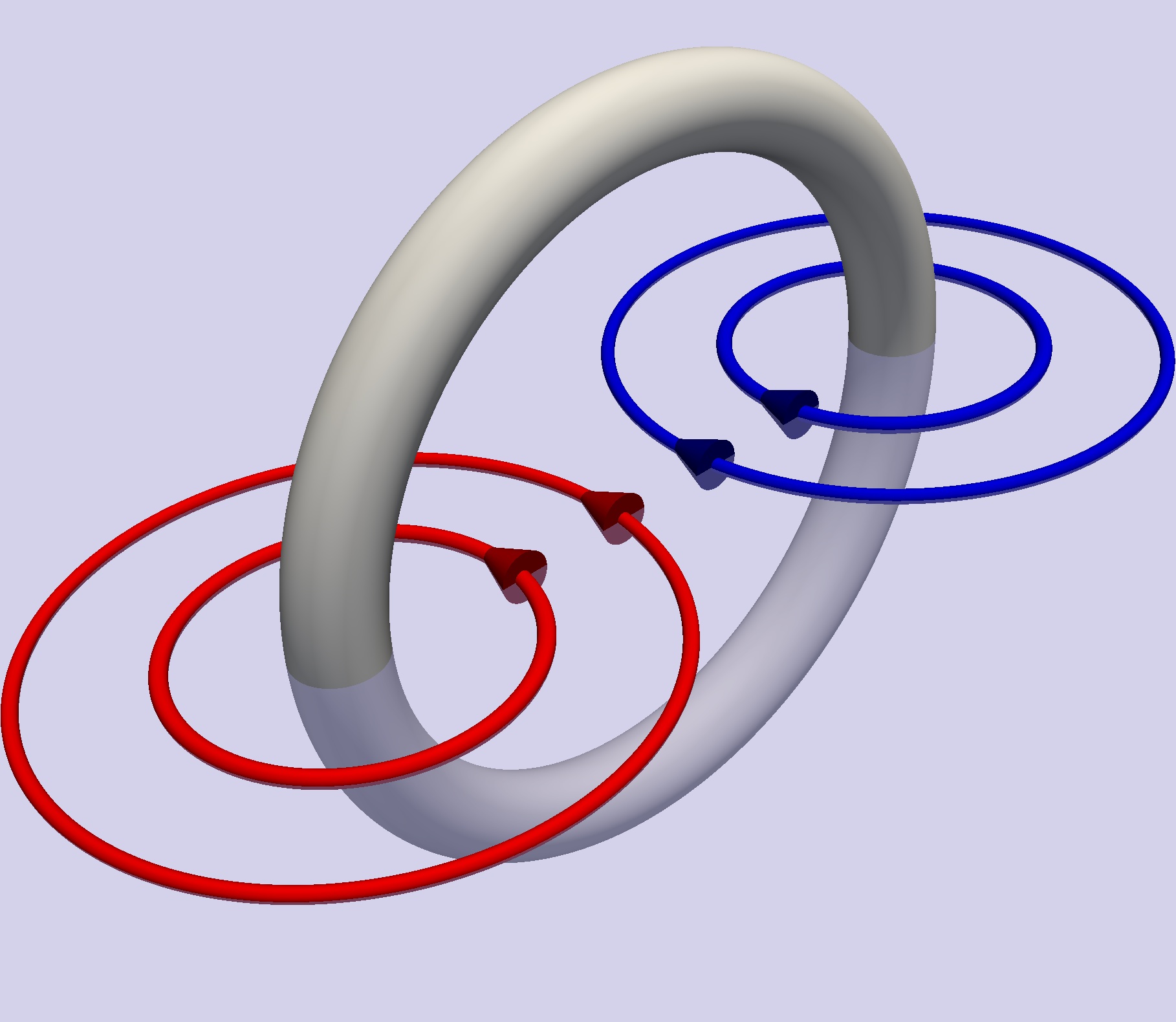
Figure 1.2: Schematic illustration of a vortex loop denoted by the gray tube. The closed arrows denote the phase winding, and the circulation of the supercurrents. Clearly, a vortex loop has no net winding at large distance.

Remark here that this derivation is essentially two-dimensional. This means that this divergence occurs in either in two dimensions or in three-dimensional systems with translation invariance along the the third direction. This is reason for the emphasis on straight vortices. In three-dimensional systems, fractional vortices oriented along the third direction have a divergent energy per unit length. So they will still be energetically penalized. On the other hand, loops of fractional vortices always have a finite energy. This can heuristically be understood as follows: As sketched in Fig. 1.2, a section of a vortex loop can be seen as pair of a vortex and an anti-vortex. In a plane such a vortex/anti-vortex pair has no net winding at large distance, so it is topologically trivial, and the energy is finite. Moreover because it is topologically trivial, there is no topological protection, so a vortex and an anti-vortex attract each other until they annihilate. Similarly, a vortex loop is topologically trivial, since it has no net winding at large distance. A vortex loop tend to collapse because of its line tension, quite similarly to a vortex/anti-vortex pair that annihilate each other.

In two-dimensions, vortices, either fractional or composite, are characterized by $\mathbb{S}^{1}\to\mathbb{S}^{1}$ topological maps. The first circle $\mathbb{S}^{1}$ denotes the closed path faraway from the vortex core (that is homeomorphic to a circle) while the second one (the target circle) corresponds to $\mathrm{U}(1)$ rotations. Heuristically, the $\mathbb{S}^{1}\to\mathbb{S}^{1}$ maps have the following meaning: they count how many times the target circle is covered while going along the closed path faraway from the vortex core (i.e. the number of phase windings). Importantly, this number can be calculated just by inspecting the closed path faraway for the vortex core. This is because the associated density of the topological invariant is a total divergence. As discussed later on, this is not the case of the extra invariants.

Depending on how the constituting fractional vortices are located relative to each other, there exist two qualitatively different ways to construct the composite topological defects. More precisely, as discussed below, the topological properties depend on whether their individual singularities overlap, or not. If the singularities do not overlap, the composite topological defect is coreless and can be characterized by an additional, topological invariant. This motivates the generic terminology of skyrmions [120]. On the other hand, if all fractional vortices are co-centred, the resulting bound state is a singular (multicomponent) vortex.

1.1.3 Additional topological properties in multicomponent systems

In addition to the winding number, which is the only topological invariant in single-component superconductors, multicomponent superconductors can be characterized by extra topological properties. As previously emphasized, the $\mathrm{U}(1)$ topological invariant is associated with the total phase winding at spatial infinity. Depending on the nature of the topological defect under consideration, the additional invariant is of different nature. If the objects considered are straight, line-like, topological defects being the bound state of straight fractional vortices, the additional invariants are given as surface integral characterizing skyrmions. If on the other hand, the objects consist of closed loops of fractional vortices, the additional invariant is given as a volume integral characterizing hopfions. Both skyrmion and hopfion numbers are discussed below. Note that while the skyrmion number is well define for any number of superconducting condensates, the hopfion number is formally defined only for two-component superconductors.

$\mathbb{C}\mathrm{P}^{N-1}$ topological invariant – Skyrmion number

The winding number, which is defined as a line integral over a closed path, is associated with the maps $\mathbb{S}^{1}\to\mathbb{S}^{1}$. It is related to the elements of the first homotopy of the circle: $n\in\pi_{1}(\mathbb{S}^{1})=\mathbb{Z}$. In contrast, multicomponent superconductors can be characterized by an additional $\mathbb{C}\mathrm{P}^{N-1}$ topological index, which is defined as an integral over the plane. Given the $N$-component complex vector $\Psi$, the $\mathbb{C}\mathrm{P}^{N-1}$ topological index is [JG21.]

$$\mathcal{Q}(\Psi)=\int_{\mathbb{R}^{2}}\frac{i\varepsilon_{ji}}{2\pi|\Psi|^{4}}\Big{[}|\Psi|^{2}\partial_{i}\Psi^{\dagger}\partial_{j}\Psi+\Psi^{\dagger}\partial_{i}\Psi\partial_{j}\Psi^{\dagger}\Psi\Big{]}dxdy\,,$$ (1.17)

where $\varepsilon$ is the Levi-Civita symbol. Provided $\Psi\neq 0$ (i.e. if singularities do not overlap), the $\mathbb{C}\mathrm{P}^{N-1}$ index $\mathcal{Q}(\Psi)$ is an integer number and it is equal to the number of flux quanta: $\mathcal{Q}(\Psi)=\int B/\Phi_{0}=n$ ($\Phi_{0}$ being the flux quantum and $n$ the number of flux quanta) [120]. It results that for a singular vortex, where all the superconducting condensates simultaneously vanish (i.e. $\Psi=0$), the skyrmion number $\mathcal{Q}(\Psi)=0$. On the other hand, if the singularities are non-overlapping (i.e. $\Psi\neq 0$), then $\mathcal{Q}(\Psi)\in\mathbb{Z}$ and the quantization condition holds. Then $\mathcal{Q}(\Psi)$ is a useful quantity that can differentiate between singular vortices and skyrmions (which are coreless defects).

It should be emphasized again that unlike the flux-quantization condition (1.14), the integral formula for the topological charge $\mathcal{Q}(\Psi)$ above is valid only for field configurations for which $\Psi$ never vanishes. The flux is still quantized for ordinary singular vortices, for which $\Psi$ vanishes, but it is no longer associated with the topological charge $\mathcal{Q}(\Psi)$, rather with the $\mathrm{U}(1)$ topological invariant related to the total phase winding at spatial infinity (the usual winding number).

Note that the topological number $\mathcal{Q}(\Psi)$ is calculated as an integral over the plane $\mathbbm{R}^{2}$. Hence it formally characterizes either two-dimensional systems ($\mathbbm{R}^{2}$), or three-dimensional systems with translation invariance normal to the plane (i.e. $\mathbbm{R}^{2}\times\mathbbm{R}$). In the later case, $\mathcal{Q}(\Psi)$ should be interpreted as a linear density of topological charge.

Hints of the demonstration:

For the rigorous derivation of the flux and topological charge quantization, see [JG21.]. Using, the definition (1.3) of the total supercurrent ${\bm{J}}$, and the relation $\mathrm{Im}(\Psi^{\dagger}{\bm{\nabla}}\Psi)=\sum_{a}|\psi_{a}|^{2}{\bm{\nabla}}\varphi_{a}$, the gauge field reads as

$${\bm{A}}=\frac{1}{e^{2}\varrho^{2}}\Big{(}{\bm{J}}-e\sum_{a}|\psi_{a}|^{2}{\bm{\nabla}}\varphi_{a}\Big{)}=\frac{1}{e^{2}\varrho^{2}}\Big{(}{\bm{J}}-e\mathrm{Im}(\Psi^{\dagger}{\bm{\nabla}}\Psi)\Big{)}\,,$$ (1.18)

where $\varrho^{2}=\sum_{a}|\psi_{a}|^{2}=\Psi^{\dagger}\Psi$ is the total superconducting density. It follows that the magnetic field can be expressed as

$$B_{k} =\frac{1}{e}\varepsilon_{kij}\left\{\partial_{i}\left(\frac{{\bm{J}}}{e\varrho^{2}}\right)-\partial_{i}\left(\sum_{a}\frac{|\psi_{a}|^{2}{\bm{\nabla}}\varphi_{a}}{\varrho^{2}}\right)\right\}$$ (1.19a)

$$=\frac{1}{e}\varepsilon_{kij}\left\{\partial_{i}\left(\frac{{\bm{J}}}{e\varrho^{2}}\right)+\frac{i}{\varrho^{4}}\left[\varrho^{2}\nabla_{i}\Psi^{\dagger}\nabla_{j}\Psi+(\Psi^{\dagger}\nabla_{i}\Psi)(\nabla_{j}\Psi^{\dagger}\Psi)\right]\right\}\,,$$ (1.19b)

where $\varepsilon_{ijk}$ is the Levi-Civita symbol. Going from the first to the second line of (1.19) is merely done by developing the second term and by eliminating the contributions that are symmetric under $i\leftrightarrow j$ (since they are contracted with the Levi-Civita symbol which is antisymmetric). Obviously the flux of ${\bm{B}}$ is quantized. Indeed, applying the Stokes theorem to the equation (1.19a) yields the relation (1.13). Now, computing the flux from the second equation (1.19b) gives

$$\Phi=\frac{1}{e^{2}\varrho^{2}}\bigointsss_{\!\!\!\!\!\!{\cal C}}{\bm{J}}\!\cdot\!d{\bm{\ell}}-\bigintsss\frac{i\varepsilon_{ij}}{e\varrho^{4}}\Big{[}\varrho^{2}\nabla_{i}\Psi^{\dagger}\nabla_{j}\Psi+(\Psi^{\dagger}\nabla_{i}\Psi)(\nabla_{j}\Psi^{\dagger}\Psi)\Big{]}dxdy\,.$$ (1.20)

Since the Meissner current vanishes asymptotically, this determines the relation between the topological charge (1.17) and the magnetic flux $\int B=\Phi_{0}\mathcal{Q}(\Psi)$ with the flux quantum $\Phi_{0}=2\pi/e$. Again one can see that $\mathcal{Q}$ is a surface integral, since the 2-form integrand is not closed.

Remark:

It is important to stress here that the definition of the magnetic field (1.19) features two contributions. The first term is the contribution from the standard superconducting currents, while the second term appears only for multicomponent system. This additional term, which involves relative density gradients and relative phase gradients, is responsible for various unusual phenomena presented later in Chapter 3.

Hopfions in two-component superconductors

The above discussion considered the topological properties of straight topological defects, where the extra invariant is calculated as a surface integral in the plane perpendicular to the vortex line. It is also possible to define an additional invariant when vortices form close loops, instead of straight defects. However, this is possible only for two-component superconductors. Topological considerations imply that knotted vortex loops in two-component superconductors are characterized by an integer topological index $\mathcal{I}$ (see, e.g. , discussions given in Refs. [37, 38, 121, 122, 123, 43, 124]). As for the previous discussion, this index is well defined when fractional vortices in the different components do not intersect ($\Psi\neq 0$). Here, the superconducting degrees of freedom are cast in a 4-dimensional unit vector ${\bm{\zeta}}=(\mathrm{Re}\,\psi_{1},\mathrm{Im}\,\psi_{1},\mathrm{Re}\,\psi_{2},\mathrm{Im}\,\psi_{2})/\sqrt{\Psi^{\dagger}\Psi}$. Note that for ${\mathbf{\zeta}}$ to be well defined, there should be no zeros of $\Psi$, i.e. no overlap between core centres of fractional vortices in both components. The finiteness of energy implies that a superconductor should be in the ground state at spatial infinity. It follows that infinity is identified with a single field configuration (up to gauge transformations). Hence, the vector field ${\bm{\zeta}}$ is a map from the one-point compactified space to the target 3-sphere ${\bm{\zeta}}:\mathbb{S}^{3}\,[\cong\mathbbm{R}^{3}\cup\{\infty\}]\to\mathbb{S}^{3}_{\Psi}$. Maps between 3-spheres fall into disjoint homotopy classes, the elements of the third homotopy group $\pi_{3}(\mathbb{S}^{3}_{\Psi})$, which is isomorphic to the integers: $\pi_{3}(\mathbb{S}^{3}_{\Psi})=\mathbb{Z}$. Hence, ${\bm{\zeta}}$ is associated with an integer number, the degree of the map ${\bm{\zeta}}$, which counts how many times the target sphere $\mathbb{S}^{3}_{\Psi}$ is wrapped while covering the whole $\mathbbm{R}^{3}$ space. Field configurations are thus characterized by the topological index

$$\mathcal{I}:=\mathrm{deg}{\bm{\zeta}}=-\frac{1}{12\pi^{2}}\int_{\mathbb{R}^{3}}\varepsilon_{ijk}\varepsilon_{abcd}\,\zeta_{a}\partial_{i}\zeta_{b}\partial_{j}\zeta_{c}\partial_{k}\zeta_{d}d{\bf r}\,,$$ (1.21)

where $\varepsilon$ is the Levi-Civita symbol. As long as ${\bm{\zeta}}$ is well defined, that is unless $\Psi$ has zeros, the index $\mathcal{I}$ is always an integer. Note that, as discussed for example in [123], the degree of ${\mathbf{\zeta}}$, $\mathcal{I}$ is equal to the Hopf charge of the combined Hopf map $h\circ{\mathbf{\zeta}}:\mathbb{S}^{3}\to\mathbb{S}^{2}$.

1.1.4 Interactions between fractional vortices

The finiteness of the energy dictates that fractional vortices cannot exist individually, and should thus form composite objects carrying an integer flux. These maybe be characterized by the additional invariant $\mathcal{Q}(\Psi)$, if $\Psi\neq 0$. To determine whether singularities overlap or not, and thus whether singular vortices or skyrmions are favoured, it is necessary at this point to determine how the fractional vortices interact together. The Ginzburg-Landau free energy describing multicomponent superconductors is a non-linear theory and thus detailed investigation of the properties of topological defects typically requires numerical simulations. However, analysing of the properties in the London limit provides valuable insight on the behaviour of the topological excitations. As demonstrated below, in the London limit, straight fractional vortices can be mapped to interacting point charges in two dimensions.

The London limit, assumes that the condensates have a constant density $|\psi_{a}|=\mathrm{const}$ everywhere, except at the small cut-off representing the vortex core. Using the Ampère’s law (1.3) to replace the current by the magnetic field in Eq. (1.12), the free energy further simplifies

$$\mathcal{F}/\mathcal{F}_{0}=\bigintsss\frac{1}{2}\left({\bm{B}}^{2}+\frac{1}{e^{2}\varrho^{2}}|{\bm{\nabla}}\!\times\!{\bm{B}}|^{2}\right)+\sum_{a,b>a}\frac{|\psi_{a}|^{2}|\psi_{b}|^{2}}{2\varrho^{2}}({\bm{\nabla}}\varphi_{ab})^{2}\,.$$ (1.22)

In principle the potential $V(\Psi,\Psi^{\dagger})$ can feature phase-locking terms that depend on the relative phase $\varphi_{ab}$ between different condensates. In the following discussion, it is assumed for simplicity that there are no such terms, and thus that the potential is simply constant and can be dismissed. The interaction energy of non-overlapping fractional vortices can be approximated, in this London limit, by considering separately the charged and neutral modes. First of all, the vector calculus identity

$$|{\bm{\nabla}}\!\times\!{\bm{B}}|^{2}={\bm{B}}\cdot{\bm{\nabla}}\!\times\!{\bm{\nabla}}\!\times\!{\bm{B}}-{\bm{\nabla}}\!\cdot\!({\bm{B}}\times{\bm{\nabla}}\!\times\!{\bm{B}})\,,$$ (1.23)

helps to rewrite the charged sector of (1.22) as

$$\mathcal{F}_{\mbox{\tiny Charged}}=\bigintsss\frac{{\bm{B}}}{2}\left({\bm{B}}+\frac{1}{e^{2}\varrho^{2}}{\bm{\nabla}}\!\times\!{\bm{\nabla}}\!\times\!{\bm{B}}\right)\,.$$ (1.24)

The London equation for a point-like vortex carrying a flux $\Phi_{a}$, and located at $\mathbf{x}_{a}$, is

$$\lambda^{2}{\bm{\nabla}}\!\times\!{\bm{\nabla}}\!\times\!{\bm{B}}+{\bm{B}}=\Phi_{a}\delta(\mathbf{x}-\mathbf{x}_{a})\,,$$ (1.25)

where $\lambda$ is the London penetration length defined as $\lambda^{-2}=e^{2}\varrho^{2}$. The corresponding solutions of the London equation (1.25) are given in terms of $K_{0}$, the modified Bessel of the second kind, as

$${\bm{B}}_{a}(\mathbf{x})=\frac{\Phi_{a}}{2\pi\lambda^{2}}K_{0}\left(\frac{|\mathbf{x}-\mathbf{x}_{a}|}{\lambda}\right)\,.$$ (1.26)

In the case of two vortices carrying fluxes $\Phi_{a}$ and $\Phi_{b}$, and located at $\mathbf{x}_{a}$ and $\mathbf{x}_{b}$, the source term in London equation reads as $\Phi_{a}\delta(\mathbf{x}-\mathbf{x}_{a})+\Phi_{b}\delta(\mathbf{x}-\mathbf{x}_{b})$, and the magnetic field is the superposition of two contributions ${\bm{B}}(\mathbf{x})={\bm{B}}_{a}(\mathbf{x})+{\bm{B}}_{b}(\mathbf{x})$. As a results, the corresponding energy of the charged sector

$$\mathcal{F}_{\mbox{\tiny Charged}} =\bigintsss\frac{1}{2}({\bm{B}}_{a}+{\bm{B}}_{b})\big{[}\Phi_{a}\delta(\mathbf{x}-\mathbf{x}_{a})+\Phi_{b}\delta(\mathbf{x}-\mathbf{x}_{b})\big{]}$$

$$=\frac{\Phi_{a}\Phi_{b}}{2\pi\lambda^{2}}K_{0}\left(\frac{|\mathbf{x}_{2}-\mathbf{x}_{1}|}{\lambda}\right)+E_{va}+E_{vb}\,,$$ (1.27)

where $E_{va}\equiv\int{\bm{B}}_{a}(\mathbf{x}_{a})\Phi_{a}/2$ stands for the (self-)energy of the vortex $a$. It results that, the interaction energy between two vortices in components $a$ and $b$ reads as

$$E^{(int),\mbox{\tiny Charged}}_{ab}=\frac{2\pi|\psi_{a}|^{2}|\psi_{b}|^{2}}{\varrho^{2}}K_{0}\left(\frac{|\mathbf{x}_{a}-\mathbf{x}_{b}|}{\lambda}\right)\,.$$ (1.28)

The interaction through the charged sector is thus a screened interaction given by the modified Bessel function. This interaction is always positive for any $a$, $b$ having the same sign of the vorticity. It then determines, a repulsive interaction between any kind of fractional vortices with co-directed winding. That is vortices, repel while a vortex and an anti-vortex attract each other. The interaction through the neutral sector, on the other hand, is attractive (resp. repulsive) for fractional vortices in the different (resp. same) components $a$ and $b$. The interaction here is logarithmic in the separation of the vortices. Note again that if there exist phase-locking potential terms, then the interaction is linear in the separation. This was for example discussed in detail, in the appendix of [JG21.]. The energy associated with the neutral sector of (1.22) reads

$$\mathcal{F}_{\mbox{\tiny Neutral}}=\sum_{a,b>a}\frac{|\psi_{a}|^{2}|\psi_{b}|^{2}}{2\varrho^{2}}\bigintsss({\bm{\nabla}}\varphi_{ab})^{2}\,.$$ (1.29)

At sufficiently large distance, a phase winding around some singularity located at the point $\mathbf{x}_{a}$, is well approximated by $\varphi_{a}=\theta$. Where here $\theta$ is the polar angle, and thus

$${\bm{\nabla}}\varphi_{a}=\frac{\bm{e}_{\theta}}{|\mathbf{x}-\mathbf{x}_{a}|}=\bm{z}\times{\bm{\nabla}}\ln|\mathbf{x}-\mathbf{x}_{a}|\,.$$ (1.30)

The interaction between fractional vortices in different condensates, respectively located at $\mathbf{x}_{a}$ and $\mathbf{x}_{b}$, is calculated as follows: Expanding the neutral sector (1.29), the interacting part reads as

$$E^{(int),\mbox{\tiny Neutral}}_{ab} =-\frac{|\psi_{a}|^{2}|\psi_{b}|^{2}}{\varrho^{2}}\bigintsss{\bm{\nabla}}\varphi_{a}\cdot{\bm{\nabla}}\varphi_{b}=\frac{|\psi_{a}|^{2}|\psi_{b}|^{2}}{\varrho^{2}}\bigintsss\varphi_{a}\Delta\varphi_{b}$$

$$=\frac{|\psi_{a}|^{2}|\psi_{b}|^{2}}{\varrho^{2}}\bigintsss\ln|\mathbf{x}-\mathbf{x}_{a}|\delta(|\mathbf{x}-\mathbf{x}_{b}|)=2\pi\frac{|\psi_{a}|^{2}|\psi_{b}|^{2}}{\varrho^{2}}\ln|\mathbf{x}_{b}-\mathbf{x}_{a}|\,.$$ (1.31)

Similarly, the interaction between two vortices in the same condensate $a$ is computed by requiring that the phase is the sum of the individual phases $\varphi_{a}=\varphi_{a}^{(1)}+\varphi_{a}^{(2)}$, while $\varphi_{b}=0$. Then the interaction reads as

$$E^{(int),\mbox{\tiny Neutral}}_{aa}=-2\pi\frac{|\psi_{a}|^{2}\sum_{c\neq a}|\psi_{c}|^{2}}{\varrho^{2}}\ln|\mathbf{x}_{a}^{(2)}-\mathbf{x}_{a}^{(1)}|\,.$$ (1.32)

Thus the interaction, via the neutral sector, between in different condensates is logarithmically attractive, while it is repulsive for vortices in the same condensate.

To summarize, noting the separation $r\equiv|\mathbf{x}_{a}-\mathbf{x}_{b}|$ and $R$ the sample’s size, the interaction energy between fractional vortices in different condensates is

$$\frac{E^{(int)}_{ab}}{2\pi}=\frac{|\psi_{a}|^{2}|\psi_{b}|^{2}}{\varrho^{2}}\Big{(}\ln\frac{r}{R}+K_{0}\left(\frac{r}{\lambda}\right)\Big{)}\,.$$ (1.33)

On the other hand, interactions between fractional vortices in the same condensates are

$$\frac{E^{(int)}_{aa}}{2\pi}=-\frac{|\psi_{a}|^{2}\sum_{c\neq a}|\psi_{c}|^{2}}{\varrho^{2}}\ln\frac{r}{R}+\frac{|\psi_{a}|^{4}}{\varrho^{2}}K_{0}\left(\frac{r}{\lambda}\right)\,.$$ (1.34)

Equations (1.33) and (1.34) thus give the different interactions between fractional vortices in different condensates. This can be illustrated in the case of a two-component superconductor. Choosing the energy scale to be $2\pi|\psi_{1}|^{2}|\psi_{2}|^{2}/\varrho^{2}$ and defining the parameter $m$ as the ratio of densities, $m=|\psi_{1}|^{2}/|\psi_{2}|^{2}$, the interaction between the fractional vortices in the various condensates reads as

$$E_{11}=\ln\frac{R}{r}+mK_{0}\left(\frac{r}{\lambda}\right)\,,\leavevmode\nobreak\ \leavevmode\nobreak\ E_{22}=\ln\frac{R}{r}+\frac{1}{m}K_{0}\left(\frac{r}{\lambda}\right)\,,\leavevmode\nobreak\ \leavevmode\nobreak\ E_{12}=-\ln\frac{R}{r}+K_{0}\left(\frac{r}{\lambda}\right)\,.$$ (1.35)

Thus, the vortex matter in the London limit of a two-component superconductor is described by a 2-parameter family $(m,R)$. Figure 1.3 shows the profiles of the different interactions (1.35) between the different kind of fractional vortices.

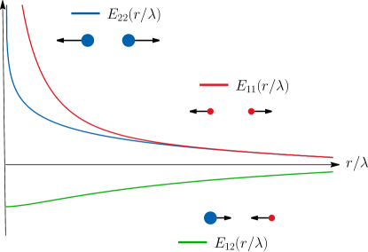
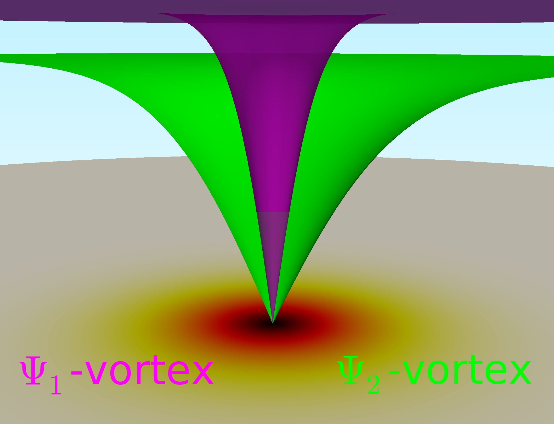
Figure 1.3: The left panel shows the interaction energies (1.35) (with $m=0.2$) between point-like charges associated with vortices in the different condensates. The blue (big) dot represents the vortex in $\psi_{1}$ while the red (small) dots represent the vortices in $\psi_{2}$. Alike charges always repel while different charges attract via the long-range logarithmic attraction. The right panel displays a schematic illustration of a composite vortex where the singularities are co-centred due to the long-range attraction between the fractional vortices in different condensates. Note that, in general, there are no reasons for the cores of different components to have same size.

Note that as $r\to 0$, the modified Bessel functions diverges as $-\ln r$. This means that for the interaction between fractional vortices in different condensates $E_{12}$, the divergence of the log term is compensated by the divergence of the Bessel function. They exactly cancel at $r=0$, as can be seen inFig. 1.3. The interaction between the vortices in the same condensates is repulsive. In multicomponent superconductors, where all condensates have the same number of vortices, the vortices in different condensates will attract each other to form a bound state of co-centered vortices that minimizes the energy cost of the neutral sector [91, 105]. As mentioned earlier, when there are phase-locking potential terms, then the attraction between fractional vortices is no more logarithmic, and it becomes linear, and the confinement becomes even stronger.

This means that, at least in the London limit, the tendency for fractional vortices (in the simplest model used here), is to simply overlap and thus to form a bound state of co-centred vortices, in order to minimize the energy of the neutral sector. Subsequently, the charged sector can be minimized by maximizing the separation between the co-centered vortices. That is by forming a triangular Abrikosov lattice of singular composite vortices. Returning to the discussion about skyrmions and vortices, this implies that superconducting condensates tend to simultaneously vanish (i.e. $\Psi=0$), and thus that the $\mathbb{C}\mathrm{P}^{N-1}$ index $\mathcal{Q}$ (1.17) is zero. As a result, forming skyrmions as lowest energy topological excitations is not a trivial task, and it typically requires additional ingredients to overcome this tendency to form co-centred composite vortices. This is discussed later in the Section 1.3.

Note that the above remarks about finiteness of the energy and interaction between fractional vortices apply for straight vortices in bulk superconducting materials. That is, the energetic divergence of the fractional vortices formally occurs only in infinite systems. Fractional vortices can yet be stabilized due to finite-size effects as for example in mesoscopic samples [91, 116, 117, 125, 103, 118]. They can also be thermodynamically stabilized near sample boundaries due to their interaction with the Meissner currents [104]. This results in a modified Bean-Livingston barrier with complex partial vortex penetration as shown in [JG17.].

Importantly, as mentioned earlier, the loops of vortices carrying a fractional flux have only a finite energy. As a result, in three dimensions loops of fractional vortices although quite energetic are still formally possible and, although dynamically unstable, can for example be thermally excited. Fractional vortex loops, actually play a central role in the critical properties of multicomponents superconductors [105, 108, 107], and superfluids [106, 109, 110].

To briefly summarize:

The elementary topological excitations in multicomponent superconductors are fractional vortices. Finite energy considerations dictate that only bound states of fractional vortices totalling an integer flux should form in bulk systems, and the intervortex interactions promote co-centered vortices. However, if the individual singularities do not overlap, such a bound state is a coreless defect called a skyrmion, and it is characterized by an additional hidden $\mathbb{C}\mathrm{P}^{N-1}$ topological invariant. Scenarii where skyrmions are favoured over singular vortices will be discussed in section 1.3. Prior to that, in the next section, it is further discussed that in the particular case of two-component systems, the topological properties of the model can also be understood using a mapping to a nonlinear $\sigma$-model.

1.2 Duality mapping to a Skyrme-Faddeev model, coupled to a massive vector ${\bm{J}}$

It is interesting to note that generic model of two-component superconductivity can be mapped to an easy-plane non-linear $\sigma$-model [121, 124]. This mapping further motivates the terminology skyrmion to denote the bound state of well separated fractional vortices. To achieve this mapping, it is first of all convenient to consider the free energy expressed in terms of charged and neutral modes (1.12). In the case of two-components, it reads as

$$\mathcal{F}/\mathcal{F}_{0}=\bigintsss\frac{{\bm{B}}^{2}}{2}+\sum_{a=1,2}\frac{1}{2}\big{(}{\bm{\nabla}}|\psi_{a}|\big{)}^{2}+\frac{{\bm{J}}^{2}}{2e^{2}\varrho^{2}}+\frac{|\psi_{1}|^{2}|\psi_{2}|^{2}}{2\varrho^{2}}({\bm{\nabla}}\varphi_{12})^{2}+V(\Psi,\Psi^{\dagger})\,.$$ (1.36)

Next, the pseudo-spin unit vector $\bm{n}$ taking value on the sphere $\mathbb{S}^{2}$, can be defined as the projection of the superconducting degrees of freedom $\Psi$ onto spin-$1/2$ Pauli matrices $\bm{\sigma}$:

$${\bm{n}}\equiv(n_{x},n_{y},n_{z})=\frac{\Psi^{\dagger}\bm{\sigma}\Psi}{\Psi^{\dagger}\Psi}\,,\leavevmode\nobreak\ \leavevmode\nobreak\ \text{where}\leavevmode\nobreak\ \leavevmode\nobreak\ \Psi^{\dagger}=(\psi_{1}^{*},\psi_{2}^{*})\,.$$ (1.37)

To rewrite the free energy (1.12) in terms of the pseudo-spin $\bm{n}$, the total density $\varrho$ and the gauge invariant current ${\bm{J}}$, the following identity is useful

$$\frac{\varrho^{2}}{4}\partial_{k}n_{a}\partial_{k}n_{a}+({\bm{\nabla}}\varrho)^{2}=\frac{|\psi_{1}|^{2}|\psi_{2}|^{2}}{\varrho^{2}}({\bm{\nabla}}\varphi_{12})^{2}+\sum_{a=1,2}({\bm{\nabla}}|\psi_{a}|)^{2}\,.$$ (1.38)

Moreover, noting the relation

$$4\varepsilon_{ijk}\partial_{i}\left(\sum_{a=1,2}\frac{|\psi_{a}|^{2}}{\varrho^{2}}\partial_{j}\varphi_{a}\right)=\varepsilon_{ijk}\varepsilon_{abc}n_{a}\partial_{i}n_{b}\partial_{j}n_{c},$$ (1.39)

together with the definition of the current (1.3), the magnetic field can be expressed as

$$B_{k}=\frac{1}{e}\varepsilon_{ijk}\left(\partial_{i}\left(\frac{J_{j}}{e\varrho^{2}}\right)-\frac{1}{4}\varepsilon_{abc}n_{a}\partial_{i}n_{b}\partial_{j}n_{c}\right)\,.$$ (1.40)

The free energy (1.36) can thus be written as

$$\frac{\mathcal{F}}{\mathcal{F}_{0}}\!=\!\bigintsss\frac{1}{2}({\bm{\nabla}}\varrho)^{2}+\frac{\varrho^{2}}{8}\partial_{k}n_{a}\partial_{k}n_{a}+\frac{{\bm{J}}^{2}}{2e^{2}\varrho^{2}}+V(\varrho,{\bm{n}})+\frac{1}{2e^{2}}\left[\varepsilon_{ijk}\left(\partial_{i}\left(\frac{J_{j}}{e\varrho^{2}}\right)-\frac{1}{4}\varepsilon_{abc}n_{a}\partial_{i}n_{b}\partial_{j}n_{c}\right)\right]^{2}\,.$$ (1.41)

In all generality, potential term $V$ depends on the total density $\varrho$ and on the pseudo-spin ${\bm{n}}$. The potential, which introduces anisotropies on the target 2-sphere, explicitly reads as

$$V(\varrho,{\bm{n}})=\frac{\varrho^{2}}{2}\big{(}a_{1}+a_{2}n_{x}\big{)}+\frac{\varrho^{4}}{4}\big{(}b_{1}+2b_{2}n_{x}+b_{3}n_{x}^{2}+b_{4}n_{z}^{2}\big{)}\,.$$ (1.42)

Depending on the values of the coefficients $a_{i}$ and $b_{i}$, the potential is either an easy-plane or an easy-axis. The explicit dependence of $a_{i}$ and $b_{i}$, on the original potential coefficients $\alpha_{ab}$ and $\beta_{abcd}$ is not very important at that point. The following relations may however be useful to identify the various coefficients

$$\varrho^{2} =|\psi_{1}|^{2}+|\psi_{2}|^{2}\,,\leavevmode\nobreak\ \leavevmode\nobreak\ \varrho^{4}=|\psi_{1}|^{4}+|\psi_{2}|^{4}+2|\psi_{1}|^{2}|\psi_{2}|^{2}\,,\leavevmode\nobreak\ \leavevmode\nobreak\ \varrho^{4}n_{z}^{2}=|\psi_{1}|^{4}+|\psi_{2}|^{4}-2|\psi_{1}|^{2}|\psi_{2}|^{2}\,,$$

$$\varrho^{4}(1-n_{z}^{2}) =\varrho^{4}(n_{x}^{2}+n_{y}^{2})=4|\psi_{1}|^{2}|\psi_{2}|^{2}\,,\leavevmode\nobreak\ \leavevmode\nobreak\ \varrho^{4}(1+n_{z}^{2})=2\big{(}|\psi_{1}|^{4}+|\psi_{2}|^{4}\big{)}\,,$$

$$\varrho^{2}n_{x} =|\psi_{1}||\psi_{2}|\cos\varphi_{12}\,,\leavevmode\nobreak\ \leavevmode\nobreak\ \varrho^{4}(n_{x}^{2}-n_{y}^{2})=|\psi_{1}|^{2}|\psi_{2}|^{2}\cos 2\varphi_{12}\,.$$ (1.43)

Topological properties:

By rewriting the theory using the dual variables, it becomes possible to provide an alternative understanding of the $\mathbb{C}\mathrm{P}^{1}$ topological charge (1.17). The pseudo-spin $\bm{n}$ (1.37) is a map from the one-point compactification of the plane ($\mathbbm{R}^{2}\cup\{\infty\}\simeq\mathbb{S}^{2}$) onto the two-sphere target space spanned by $\bm{n}$. That is ${\bm{n}}:\mathbb{S}^{2}\to\mathbb{S}^{2}$, which is classified by the homotopy class $\pi_{2}(\mathbb{S}^{2})\in\mathbb{Z}$, thus defining the topological invariant

$$\mathcal{Q}({\bm{n}})=\frac{1}{4\pi}\int_{\mathbbm{R}^{2}}{\bm{n}}\cdot\partial_{x}{\bm{n}}\times\partial_{y}{\bm{n}}\,\,dxdy\,.$$ (1.44)

As before, since $\bm{n}$ is ill-defined when $\Psi=0$, ordinary (composite) singular vortices, have $\mathcal{Q}({\bm{n}})=0$. Core-split vortices, on the other hand, have an integer topological charge $\mathcal{Q}({\bm{n}})\in\mathbb{Z}$ which coincides with the number of carried flux quanta. In a way, $\mathcal{Q}({\bm{n}})$ counts the number of times the pseudo-spin texture of ${\bm{n}}$ wraps the target two-sphere. It is worth emphasizing that the topological charge (1.44) is an integer, when integrated over the infinite plane $\mathbbm{R}^{2}$, or at least an large enough domain $\Omega\subset\mathbbm{R}^{2}$.

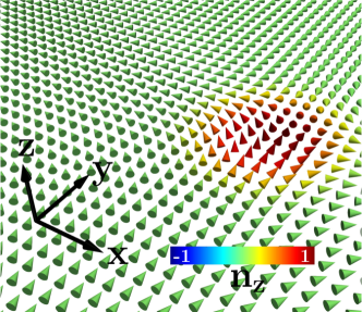
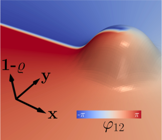
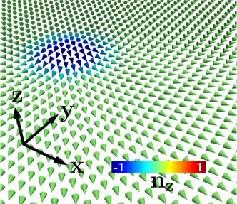
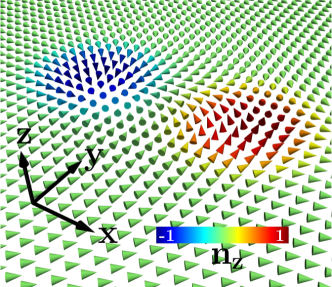
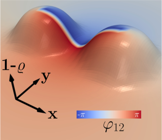
Figure 1.4: Illustration of (anti-)merons and skyrmion solutions. The left panels show the pseudo-spin $\bm{n}$ calculated from the Ginzburg-Landau quantities, using the relation (1.45). The arrows show $\bm{n}$ and the color scale encodes the value of $n_{z}$. The right panels display the corresponding Ginzburg-Landau quantities. Namely the elevation of the surface stems for the density depletion $1-\varrho$, while the colouring indicates the value of the relative phase $\varphi_{12}$.

Pseudo-spin textures. Skyrmions and Merons:

The core-split vortices thus have a skyrmionic character, with a topological charge $\mathcal{Q}({\bm{n}})\in\mathbb{Z}$. In terms of the degrees of freedom of the two-component Ginzburg-Landau theory (1.36), the pseudo-spin reads as

$${\bm{n}}=\left(\frac{2|\psi_{1}||\psi_{2}|}{|\psi_{1}|^{2}+|\psi_{2}|^{2}}\cos\varphi_{12},\frac{2|\psi_{1}||\psi_{2}|}{|\psi_{1}|^{2}+|\psi_{2}|^{2}}\sin\varphi_{12},\frac{|\psi_{1}|^{2}-|\psi_{2}|^{2}}{|\psi_{1}|^{2}+|\psi_{2}|^{2}}\right)\,.$$ (1.45)

From this, it is obvious that the core of a vortex in $\psi_{1}$ maps to ${\bm{n}}=(0,0,-1)$, while a core in $\psi_{2}$ gives ${\bm{n}}=(0,0,1)$. The vortex cores thus map to the poles of the target sphere.

Moreover, the pseudo-spin associated to a single fractional vortex covers only half of the target sphere. Such configurations are sometimes called merons. More precisely, a fractional vortex in $\psi_{2}$ covers only the north hemisphere is a meron, while a vortex $\psi_{1}$ covers only the south hemisphere is an anti-meron. This interpretation of the fractional vortices as (anti-)merons is displayed in Fig. 1.4. Since the pseudo-spin do not wrap entirely the target two-sphere, the associated topological charge (1.44) is trivial: $\mathcal{Q}({\bm{n}})=0$. Both the pseudo-spin and the Ginzburg-Landau quantities show that the relative phase have a net winding, and thus have divergent energy as discussed earlier.

The last line of figure 1.4 displays a skyrmion configuration corresponding to core-split vortices. The skyrmion, which is a bound state of non-overlapping fractional vortices, can be seen as the bound state of a meron and an anti-meron. Unlike merons, a skyrmion do not have a net winding of the relative phase $\varphi_{12}$. Thus skyrmions, have finite energy. Moreover, the pseudo-spin of a skyrmion do wrap entirely the target two-sphere. It follows that the associated topological charge (1.44) is integer, here $\mathcal{Q}({\bm{n}})=1$.

Note that the configurations that are displayed here, are only illustrations of the topological properties of (anti-)merons and skyrmion configurations. They are configurations with the appropriate topological properties, but they are not solutions (i.e. minima) of the Ginzburg-Landau theory (1.36). Indeed, as discussed earlier, the fractional vortices in the different components (and thus the merons and anti-merons) typically attract each other. Because of the attraction, merons and anti-merons can annihilate, thus converting a skyrmion into a singular vortex where the individual singularities superimpose. Yet, as discussed in the next section, there can exist various mechanism to stabilize skyrmions.

1.3 Existence of skyrmions and exotic vortex states

To summarize briefly, and repeat the topological properties presented in the above sections, the elementary topological excitations in multicomponent superconductors are fractional vortices. That is, field configurations with independent phase windings in either of the components, which carry only a fraction of the elementary flux quantum $\Phi_{0}$. Because they have a winding of the relative phase between the different components, fractional vortices have divergent energy per unit length. Thus finite energy requirements dictate that composite vortices (i.e. bound states of fractional vortices in each component) are the only configurations with finite energy per unit length. As a result these composite vortices, carrying an integer flux quantum, are the only configurations that can form in bulk multicomponent superconductors. Depending on the relative positions of the individual singularities, the resulting composite vortex is either termed singular, if the singularities are superimposed, or coreless, if they do not. Composite coreless vortices are characterized by the additional topological invariant associated with the complex projective space $\mathbb{C}\mathrm{P}^{N-1}$ (1.17). The existence of the additional invariant motivates the terminology skyrmion to denote a coreless vortex. The propensity to form either singular or coreless vortices depends on the interaction energy between the fractional vortices. The London limit calculations, in the most elementary case, state that fractional vortices are logarithmically bound and that the interaction energy is minimized when they superimpose. This raises the natural question of whether the skyrmions (the coreless vortices) can form at all, and be favoured compared to (Abrikosov) singular vortices? In other word is there a mechanism that provides a short-range repulsion between the fractional vortices, so that they form a bound state with a finite separation? Note that composite singular defects still feature interesting new properties. These are discussed later in Chapter 2.

So, in order to form skyrmions, a stabilizing mechanism is needed to counteract the tendency of the singularities to superimpose. It turns out that there exist various ways to circumvent the confinement of fractional vortices. For example this can originate in non-linear effects beyond the London approximation, or by additional interacting terms in the free energy. It follows that, despite the naive arguments, skyrmions actually exist in many superconducting systems. These mechanisms that enforce the core-splitting, stabilize skyrmions against collapsing into a singular Abrikosov vortex. One could alternatively say that because of the extra terms, the Abrikosov vortex is unstable and decay into a coreless defect: a skyrmion. Various possibility are detailed below.

1.3.1 Skyrmions in mixtures of commensurately charged condensates

Typically, in condensed matter systems the multiple superconducting condensates are coupled to the gauge field via the same gauge coupling which is the charge of the Cooper pairs (twice the charge of their constituent fermion). Still, it is formally possible to consider the case of a mixture of condensates with different electric charges. Such a situation is expected to appear for example in the superconducting state of liquid metallic deuterium, where the deuteron is a charge-$1$ boson which can form a Bose-Einstein condensate, that coexists with the Cooper pairs of electrons and/or protons [67, 68, 126]. The Bose-Einstein condensate of deuterons carries only once the charge of its constituent boson, while Cooper pairs carry twice the charge of their constituent fermion. There, the electronic Cooper pairs carry a charge $-2e$ while the Bose-Einstein condensate of deuteron carries an electric charge $+e$. Interestingly, the flux quantization and finite energy considerations similar to that discussed in the Section 1.1, dictate that the electric charges should be commensurate, for the vortex solutions to have finite energy [JG18.]. This implies that the composite vortices carrying an integer flux quantum are bound states of a different number of fractional vortices in both components. Moreover, the resulting bound state is typically a core-less defect, and these skyrmions can be characterized by a pseudo-spin texture, and by a hidden $\mathbb{C}\mathrm{P}^{1}$ invariant similar to those discussed above. This was analyzed in details in [JG18.].

To account for the possibility to have a mixture of two superconducting condensates carrying different charges, the gauge derivative in the kinetic term is chosen to have different gauge couplings for the two individual condensates: ${\bm{D}}\psi_{a}=({\bm{\nabla}}+ie_{a}{\bm{A}})\psi_{a}$ (here $a=1,2$). The individual gauge couplings are conveniently parametrized as $e_{a}=eg_{a}$ where $g_{a}$ are integer numbers $g_{a}\in\mathbb{Z}$, and $e$ fixes the scale of the electric charges. Applying this parametrization to liquid metallic deuterium, the couplings are $(g_{1},g_{2})=(1,2)$ and $\psi_{1}$ stands for the deuteron condensate while $\psi_{2}$ (carrying twice the electric charge of $\psi_{1}$) denotes the electronic Cooper pairs. When considering the possibility that the condensates can have different charges, via the redefinition of the gauge derivative, the superconducting current (1.4) reads as ${\bm{J}}=e\sum_{a}g_{a}|\psi_{a}|^{2}({\bm{\nabla}}\varphi_{a}+eg_{a}{\bm{A}})$. Since the supercurrent ${\bm{J}}$ is screened and that it decays exponentially, the magnetic flux (1.14) reads as

$$\Phi=\frac{-1}{e\sum_{b}g_{b}^{2}|\psi_{b}|^{2}}\bigointsss_{\!\!\!\!\!\!{\cal C}}\sum_{a}g_{a}|\psi_{a}|^{2}{\bm{\nabla}}\varphi_{a}\!\cdot\!d{\bm{\ell}}=\frac{\Phi_{0}\sum_{a}g_{a}|\psi_{a}|^{2}}{2\pi\sum_{b}g_{b}^{2}|\psi_{b}|^{2}}\bigointsss_{\!\!\!\!\!\!{\cal C}}{\bm{\nabla}}\varphi_{a}\!\cdot\!d{\bm{\ell}}\,,$$ (1.46)

where $\Phi_{0}=2\pi/e$ is the flux quantum and the closed integration path is chosen for the flux to be positive. The condensates $\psi_{a}$ being complex fields, they wind an integer number of time, and $(n_{1},n_{2})$ denotes the field configurations with the winding $n_{a}$ of the condensate $\psi_{a}$. A fractional vortex in the condensate $a$ carries a fraction $\Phi_{a}/\Phi_{0}=g_{a}|\psi_{a}|^{2}/\sum_{b}g_{b}^{2}|\psi_{b}|^{2}$ of the magnetic flux. As long as $g_{1}\neq g_{2}$, the condition for the quantization of the flux, is that each condensate should wind $n_{a}=g_{a}$ times. This follows from

$$\sum_{a}n_{a}\frac{\Phi_{a}}{\Phi_{0}}=\frac{\sum_{a}n_{a}g_{a}|\psi_{a}|^{2}}{\sum_{b}g_{b}^{2}|\psi_{b}|^{2}}=1\,,\leavevmode\nobreak\ \leavevmode\nobreak\ \leavevmode\nobreak\ \text{iff}\leavevmode\nobreak\ \leavevmode\nobreak\ n_{a}=g_{a}\,.$$ (1.47)

A separation into charged and neutral modes, similar to that derived above (1.12), dictates that only the configurations that carry an integer flux ($n_{a}=g_{a}$) have finite energy [127]. This can be seen by requiring the absence of logarithmic divergence, and thus that the neutral mode has no winding

$$0=\bigointsss_{\!\!\!\!\!\!{\cal C}}{\bm{\nabla}}(g_{1}\varphi_{2}-g_{2}\varphi_{1})\!\cdot\!d{\bm{\ell}}=(g_{1}n_{2}-g_{2}n_{1})\,.$$ (1.48)

For a configuration carrying a single flux quantum (and since $g_{a}$ and $n_{a}$ are integers), this implies that $n_{a}=g_{a}$. Thus the finite energy configurations winds $g_{1}$ times in $\psi_{1}$ and $g_{2}$ times in $\psi_{2}$. Note that this condition implies that the total flux is integer (1.47). On the other hand, when $g_{1}n_{2}-g_{2}n_{1}\neq 0$, the screening is incomplete and the associated energy grows with the system size. Such vortex configurations are thus thermodynamically unstable in bulk systems.

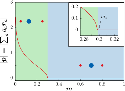
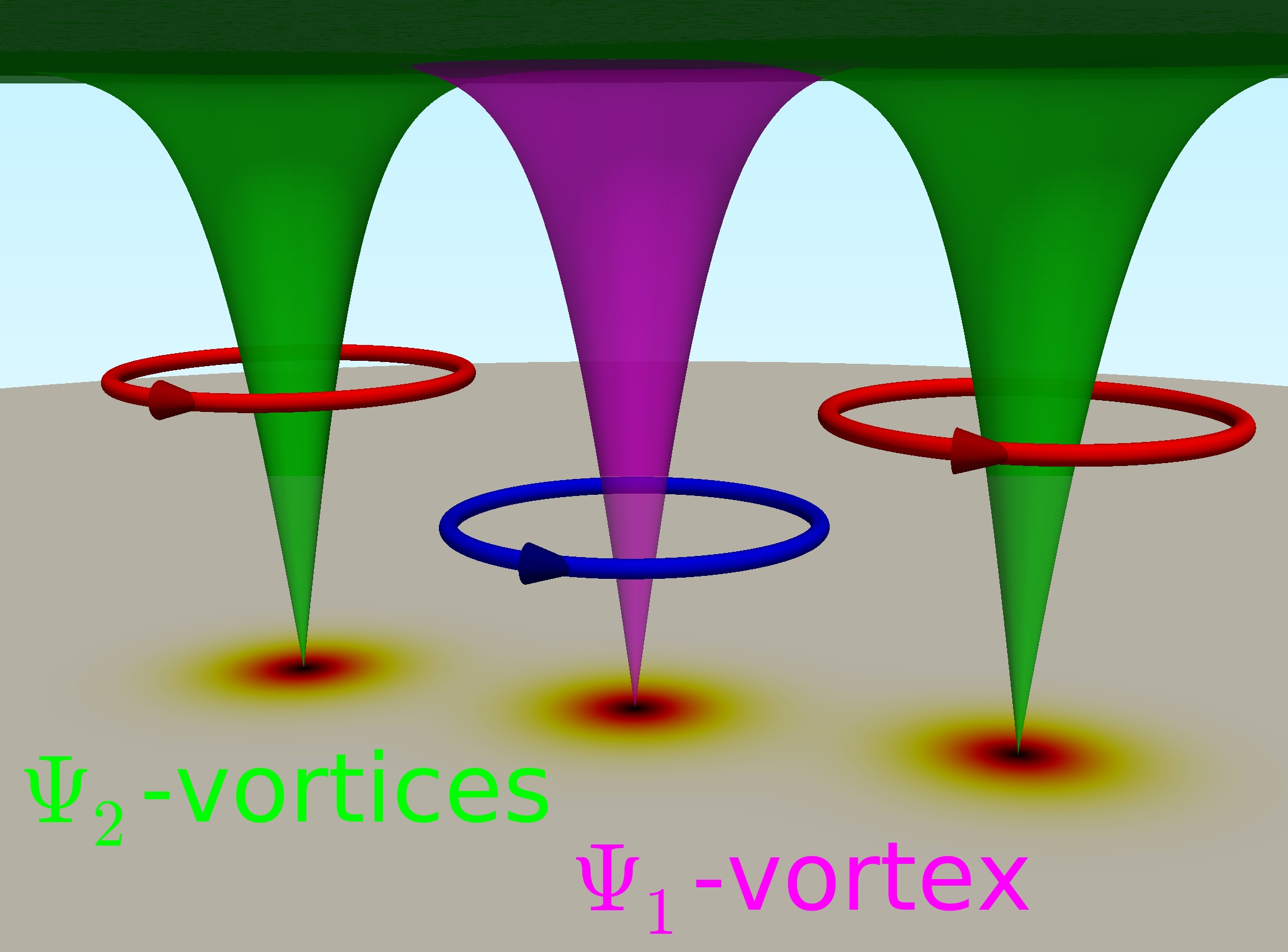
Figure 1.5: The left panel shows the structure of a single skyrmion (thus corresponding to the charges $g_{1}=1$ and $g_{2}=2$), obtained by minimizing the corresponding interaction energy (1.49). It shows the parametric dependence of the dipole moment defined in point charges mapping with charges $q_{2}=g_{1}$ and $q_{1}=-g_{2}$. The composite vortex structure undergoes a phase transition from a dipolar phase below $m_{\star}$ to a quadrupolar phase. The right panel displays a schematic illustration of the a composite vortex with a single fractional vortex in the condensate $\psi_{1}$ bound with two vortices in $\psi_{2}$.

The condensates with different charges favour bound states of fractional vortices with a finite separation, unlike the inter-vortex interaction derived in Section 1.1.4 [JG18.]. Indeed, similar calculation shows that the intervortex interactions are characterized by the ratio of the charges in the different condensates $s=\frac{g_{1}}{g_{2}}$. The interaction between fractional vortices reads as

$$E_{11}=\frac{1}{s}\ln\frac{R}{r}+\frac{m}{s}K_{0}\left(\frac{r}{\lambda}\right)\,,\leavevmode\nobreak\ \leavevmode\nobreak\ E_{22}=s\ln\frac{R}{r}+\frac{s}{m}K_{0}\left(\frac{r}{\lambda}\right)\,,\leavevmode\nobreak\ \leavevmode\nobreak\ E_{12}=-\ln\frac{R}{r}+K_{0}\left(\frac{r}{\lambda}\right)\,.$$ (1.49)

It follows that the vortex matter in the London limit of a two-component superconductor with incommensurate charges is described by a 3-parameter family $(m,s,R)$. The individual interactions are thus similar to that illustrated in Fig. 1.3, and that vortices in different condensates attract each other to form a bound state of co-centered vortices while vortices in the same condensate always repel each other. However, since both condensates have a different number of fractional vortices, the system has to compromise between the fact that vortices in the different condensates tend to overlap, while vortices in similar condensates repel each other. As illustrated in Fig. 1.5, the integer flux carrying defect is thus a molecule-like bound state of split fractional vortices.

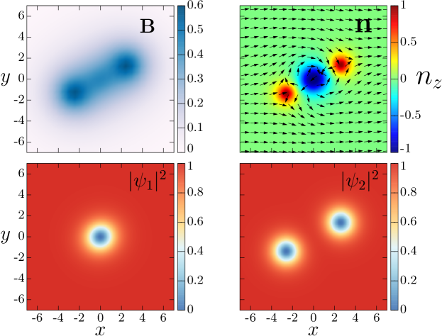
Figure 1.6: Molecule-like topological excitations carrying a single flux quantum, for the different couplings $(g_{1},g_{2})=(1,2)$. The parameters of the Ginzburg-Landau energy (1.50) are $\alpha_{aa}=-1$, $\beta_{aa}=1$ , and $e=0.2$. The displayed quantities on the top row are the magnetic field ${\bm{B}}$ and the pseudo-spin $\bm{n}$. The bottom row shows the densities of the two components $|\psi_{a}|^{2}$.

Skyrmions beyond the London limit.

The analysis in the London limit predicts the existence of coreless topological defects with different number of vortices in the different condensates. The analysis beyond the London approximation requires to specify the potential for the Ginzburg-Landau energy (1.12), as for example

$$V(\Psi,\Psi^{\dagger})=\sum_{a=1}^{2}\left(\alpha_{aa}|\psi_{a}|^{2}+\frac{\beta_{aa}}{2}|\psi_{a}|^{4}\right)\,.$$ (1.50)

The coreless vortex solutions are obtained by minimizing the Ginzburg-Landau energy with a suitable initial guess (see the numerical methods in the Appendix B). These solutions do exist beyond the London approximation, as can be seen in Figure 1.6. This is the simplest excitations carrying a unit flux quantum, for different couplings $(g_{1},g_{2})=(1,2)$.

Many other solutions for various couplings $(g_{1},g_{2})$, and the possible relevance to describe superconducting state for liquid metallic deuterium (LMD), were considered in [JG18.]. This model of two-condensates with arbitrary charges was generalized, together with the spectrum of the topological excitation in [128].

Topological properties.

The two-component model with different charges, feature similar properties than the usual two-component model. However, because of the different gauge couplings, the superconducting degrees of freedom should be collected as

$$\Psi^{\dagger}=\left(\psi_{1}^{*g_{2}},\psi_{2}^{*g_{1}}\right)\,.$$ (1.51)

Provided this modification, the charge $\mathcal{Q}(\Psi)$ (1.17), projection to the pseudo-spin $\bm{n}$ (1.37), and the associated charge $\mathcal{Q}(\bm{n})$ (1.44) are still valid.

1.3.2 Skyrmions and hopfions stabilized by the Andreev-Bashkin effect

The dissipationless inter-component drag, known as the Andreev-Bashkin effect [129], is a generic interaction in multicomponent superconductors and superfluids, but it is often neglected. Namely, in superfluid mixtures with two components, the current of a given component ${\bm{j}}_{1,2}$ generically depends on both superfluid velocities ${\bm{v}}_{1,2}$. This is due to the inter-component interactions occurring between particles, and the relations between currents and velocities are:

$${\bm{j}}_{1}=\rho_{11}{\bm{v}}_{1}+\rho_{12}{\bm{v}}_{2}\,,\leavevmode\nobreak\ \leavevmode\nobreak\ \leavevmode\nobreak\ \text{and}\leavevmode\nobreak\ \leavevmode\nobreak\ \leavevmode\nobreak\ {\bm{j}}_{2}=\rho_{22}{\bm{v}}_{2}+\rho_{21}{\bm{v}}_{1}\,.$$ (1.52)

The off-diagonal coefficients $\rho_{12}$ and $\rho_{21}$ determine the fraction of the density of one of the superfluid components carried by the superfluid velocity of the other. They thus describe the inter-component drag. The inter-component coefficients $\rho_{ab}$ can be large (compared to the intra-component coefficients $\rho_{aa}$), for example in strongly correlated systems [130, 131, 132], Fermi-liquids mixtures [133, 134], or in spin-triplet superconductors and superfluids [135]. More general drag interactions, the dissipationless vector drag, where recently argued to be occur in certain kind of optical lattices [136].

The dissipation-less drag (1.52), in a two-component model of superconductivity, can be accounted for by adding current-current interaction

$$\cdots+\sum_{a,b=1,2}\frac{\mu_{ab}}{2}{\bm{J}}_{a}\cdot{\bm{J}}_{b}+\cdots\,,$$ (1.53)

to the generic Ginzburg-Landau free energy density. This was discussed in details for example in [137, 138]. There, ${\bm{J}}_{a}=\mathrm{Im}(\psi_{a}^{*}{\bm{D}}\psi_{a})$, stands for the individual currents in the absence of drag. The off-diagonal coefficients $\mu_{12}=\mu_{21}$ of the current coupling matrix $\hat{\mu}$ describe the intercomponent drag. The total current, which is the sum of the individual supercurrents, have a similar structure to that described in (1.52). For now, assuming the absence of mixed-gradient terms in the free energy (1) (coefficients $\kappa_{ab}=0$ if $a\neq b$). When adding the current-current interactions (1.53), the total current reads as:

$${\bm{J}}/e=\sum_{a}w_{a}|\psi_{a}|^{2}({\bm{\nabla}}\varphi_{a}+e{\bm{A}})\,,\leavevmode\nobreak\ \leavevmode\nobreak\ \text{where}\leavevmode\nobreak\ \leavevmode\nobreak\ \leavevmode\nobreak\ w_{a}=\kappa_{aa}+\sum_{b}\mu_{ab}|\psi_{b}|^{2}\,.$$ (1.54)

The role of $w_{a}$ is to re-weight the individual currents. More precisely, the charged and neutral modes in (1.12) are renormalized differently due to the inter-component drag.

An analysis of the inter-vortex interaction, similar to that derived in Section 1.1.4, shows that the fractional vortices should form a bound state with a finite separation [JG20.]. Namely, in the London limit, the intervortex interactions (1.35) are characterized by two additional parameters $w>1$ and $m>0$, that depend on the drag. In the case where $\mu_{11}=\mu_{22}=\mu_{12}\equiv\mu$, the interaction between the fractional vortices in the various condensates reads as [137]:

$$E_{11}=\ln\frac{R}{r}+mwK_{0}\left(\frac{r}{\lambda}\right)\,,\leavevmode\nobreak\ \leavevmode\nobreak\ E_{22}=\ln\frac{R}{r}+\frac{w}{m}K_{0}\left(\frac{r}{\lambda}\right)\,,\leavevmode\nobreak\ \leavevmode\nobreak\ E_{12}=-\ln\frac{R}{r}+wK_{0}\left(\frac{r}{\lambda}\right)\,.$$ (1.55)

Here, $w=1+\mu\varrho^{2}$, $m=|\psi_{1}|^{2}/|\psi_{2}|^{2}$ and $\lambda^{-1}=e\sqrt{w\varrho^{2}}$. $R$ stands for the system size and $\varrho^{2}=\sum_{a}|\psi_{a}|^{2}$ is the total density. Thus the vortex matter in the London limit of a two-component superconductor with dissipationless drag is described by a 3-parameter family $(m,w,R)$. The figure 1.7 shows the profiles of the different interactions (1.55) between the different kind of fractional vortices. Because of the additional parameter $w$, the repulsive and attractive contributions in $E_{12}$ do not compensate at $r=0$ any longer. Instead, they cancel at a finite separation, so that even in the London limit, the interactions tend to form skyrmions.

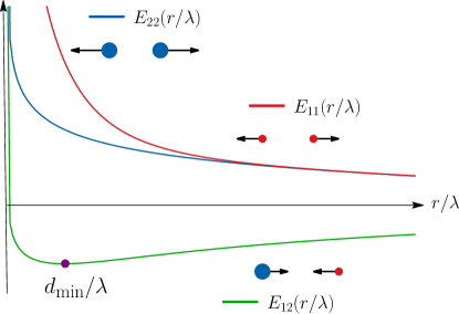
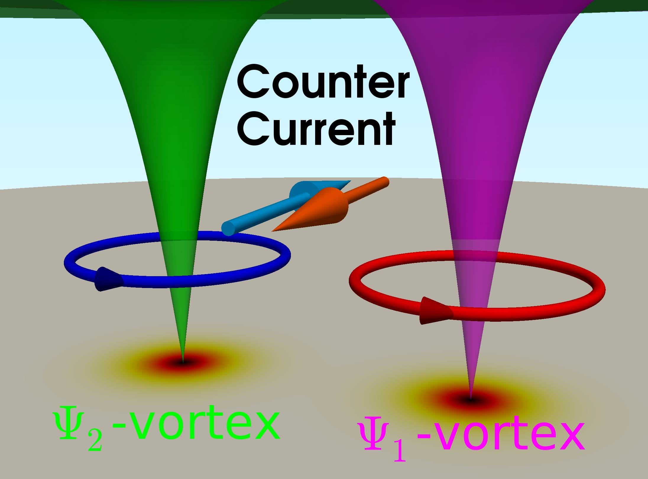
Figure 1.7: The left panel shows the interaction energies (1.55) (with $m=0.2$, $w=1.8$) between the point-like charges associated with vortices in different condensates. The blue (big) dot represents the vortex in $\psi_{1}$ while the red (small) dots represent the vortices in $\psi_{2}$. Alike charges always repel, while different charges interact with a long-range logarithmic attraction, and a short-range repulsion. The right panel displays a schematic illustration of the Andreev-Bashkin effect in a composite vortex

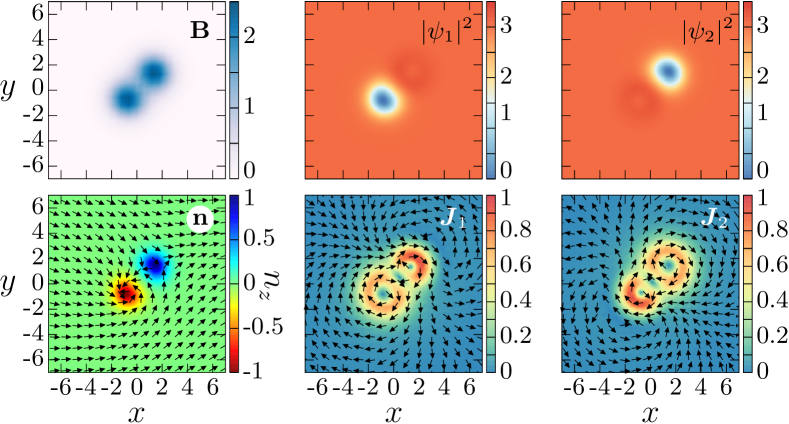
Figure 1.8: A skyrmion solution of two-component superconductor with dissipationless drag interaction (1.53), with the couplings $\mu_{11}=\mu_{22}=\mu_{12}=2$. The parameters of the simple potential interaction (1.50) are $(\alpha_{aa},\beta_{aa})=(-3,1)$, and the gauge coupling is $e=0.2$. The displayed quantities on the top left panel is the magnetic field. The other panels on the top row, show the individual densities of the superconducting condensates $|\psi_{1}|^{2}$ and $|\psi_{2}|^{2}$. This is clearly a coreless defect, since both singularities do not overlap. The bottom left panel shows the associated pseudo-spin texture $\bm{n}$ (1.37), while the other panels on the bottom row, are the individual currents ${\bm{J}}_{a}$.

Skyrmions beyond the London limit:

Physically the drag term $\mu_{12}{\bm{J}}_{1}\cdot{\bm{J}}_{2}$, promotes counter-flow compared to co-flowing currents. More precisely, the Andreev-Bashkin term gives a penalty on co-directed currents ${\bm{J}}_{1}$ and ${\bm{J}}_{2}$ (when $\mu_{12}>0$). Note that, as illustrated in Fig. 1.7, if the individual singularities do not overlap, the region in-between features counter-directed currents. It follows that the drag term (when $\mu_{12}>0$) reduces the energy of the configuration by maximizing the region where individual currents are counter-directed. Hence the Andreev-Bashkin term promotes the region of counter-directed currents and thus favours core-splitting.

The above calculations in the London limit thus predict that fractional vortices form a bound state where the individual singularities do not overlap. As illustrated in the Figure 1.8, such solutions also exist beyond the London approximation (see more examples in [JG20.]). The panels showing the individual densities clearly demonstrate that the numerically obtained solution feature non-overlapping vortices in both components. Moreover, the drag effect appears clearly from the panels showing the individual currents. Indeed, the Fig. 1.8 shows that the vortex in $\psi_{1}$ induces a non-zero circulating current in $\psi_{2}$. This can be seen by defining the supercurrent associated with a given condensate

$${\bm{J}}_{a}/e=\left(1+\mu|\psi_{a}|^{2}\right)\mathrm{Im}(\psi_{a}^{*}{\bm{D}}\psi_{a})+\mu|\psi_{a}|^{2}\mathrm{Im}(\psi_{b}^{*}{\bm{D}}\psi_{b})\,,\leavevmode\nobreak\ \leavevmode\nobreak\ \leavevmode\nobreak\ \text{with}\leavevmode\nobreak\ \leavevmode\nobreak\ b\neq a\,.$$ (1.56)

As demonstrated in [JG20.], the two-component model with dissipationless drag interaction (1.53), can be mapped to a Skyrme-Faddeev model similarly to the discussion in Section 1.2:

$$\frac{\mathcal{F}}{\mathcal{F}_{0}}\!=\!\bigintsss\frac{1}{2}({\bm{\nabla}}\varrho)^{2}+\frac{\varrho^{2}}{8}\partial_{k}n_{a}\partial_{k}n_{a}+\frac{{\bm{J}}^{2}}{2we^{2}\varrho^{2}}+V(\varrho,{\bm{n}})+\frac{1}{2e^{2}}\left[\varepsilon_{ijk}\left(\partial_{i}\left(\frac{J_{j}}{we\varrho^{2}}\right)-\frac{1}{4}\varepsilon_{abc}n_{a}\partial_{i}n_{b}\partial_{j}n_{c}\right)\right]^{2}.$$ (1.57)

The difference with the mapping (1.41) is the role of $w=1+\mu\varrho^{2}$ that renormalizes the terms involving the total current ${\bm{J}}$. The coreless vortices are thus characterized, as compared to singular vortices, by the additional topological charge $\mathcal{Q}(\Psi)$ (1.17) or $\mathcal{Q}({\bm{n}})$ (1.44) that is quantized with $\mathcal{Q}=n$ (with $n$ being the number of carried flux quanta). Numerically calculated topological charge is found to be integer (with typical error of order $10^{-4}-10^{-5}$).

The pseudo-spin texture $\bm{n}$ (1.37) of the corresponding skyrmion tube is also displayed on the bottom left panel in the Figure 1.8. The skyrmion here consists of one meron and an anti-meron, standing for the fractional vortices in the individual components, similar to those illustrated in Fig. 1.4. The mapping of the fractional vortices to point particles suggests the existence of long-range inter-skyrmions dipolar forces. Indeed, this mapping interprets the fractional vortices as point particles with opposite charges. A bound state of such charges thus features a dipole moment as well. The detailed analysis of the two-component $\mathrm{U}(1)\!\times\!\mathrm{U}(1)$ superconductors with interspecies dissipationless drag, in Ref. [JG20.], confirmed this by various numerical simulations, in the full Ginzburg-Landau regime.

The magnetic field of these skyrmions, as can be seen in Fig. 1.8, is different from that of singular vortex. Moreover, the interaction between vortices is long-ranged dipolar [137]. This results in an unconventional magnetic response in low fields which features vortex lattices lacking the conventional hexagonal structure. Importantly, the magnetization process, as well shows unconventional properties with square lattice growing inward from boundaries of the sample [JG20.]. Such unusual properties can in principle be identified easily for example in scanning SQUID measurements.

Hopfions beyond the London limit:

The intuition suggests that twisted loops of such skyrmions might have much more complicated interaction, and possibly would not completely decay, as the loops of conventional vortices do. Such a twisted skyrmion loop consists of braided closed loops of fractional vortices. The numerical minimization, starting from various initial states of knotted and linked vortex loops, demonstrate that knotted vortices can indeed be stabilized because of the Andreev-Bashkin terms [JG4.]. These simulations are, in a way, related to the relaxation processes of vortex tangles formed due to fluctuations. Indeed, in the absence of an external field, closed loops form dynamically, for example due to quenches or to thermal fluctuations. Thus the superconducting state here can support an infinite number of (meta-)stable solutions corresponding to topologically different ways to tie vortex knots. The Figure 4 shows $10$ stable knotted vortex loops, termed hopfions, with the smallest values of the topological index $\mathcal{I}$ (1.21).

Note that unlike the previously discussed skyrmions, the hopfions here are characterized only by the hidden topological invariant $\mathcal{I}$ (1.21). Indeed the skyrmions, which are straight topological defects, are characterized by the global $\mathrm{U}(1)$ charge (the total winding) and by the additional topological charge $\mathcal{Q}(\Psi)$ (1.17) or $\mathcal{Q}({\bf n})$ (1.44). Knots on the other hands are trivial regarding the $\mathrm{U}(1)$ charge (the total winding is zero), while the degree $\mathcal{I}$ (1.21) is an integer.

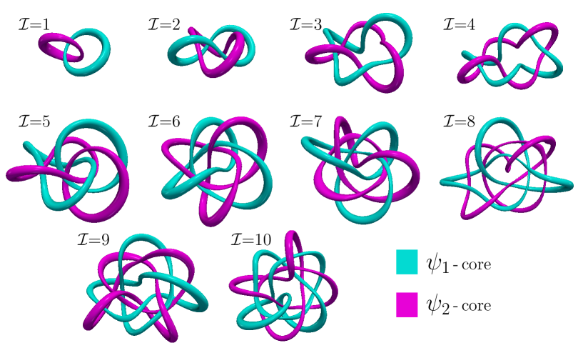
Figure 1.9: Solutions for stable knots with topological charges $\mathcal{I}$=1-10. The various panels display the core structure where the cyan and magenta tubes are surfaces enclosing the cores of the fractional vortices in each component. When increasing the index $\mathcal{I}$, the topological structure of the vorticity becomes increasingly more complex.

The knotted solutions displayed in Fig. 4 are represented by their core structure, and labelled by the corresponding value of invariant $\mathcal{I}$ (1.21). The cyan and magenta tubes enclose the singularities in the different condensates, and thus indicate the core structure. The knotted solutions are also characterized by a complicated structure of knotted lines of the magnetic field ${\bm{B}}$. These are not displayed here, but can be found from [JG4.]. The solutions with $\mathcal{I}=1-4$ consist of two fractional vortex loops, linked together and twisted around each other a varying number of times. The solution with $\mathcal{I}=5$ is a bound state of two pairs of linked fractional vortex loops, and $\mathcal{I}=6$ consists of two linked trefoil knots. In all these configurations, there is a symmetry of exchanging the cores of the different condensates. Interestingly, for higher values of the topological index $\mathcal{I}=7-10$, the vorticity of the different components are inequivalent, and this symmetry is no longer available. For example, the $\mathcal{I}=7$ knot consists in a trefoil knot in one component, linked to two twisted fractional vortex loops of the other component. These solutions thus form some kind of isomers.

In contrast to the London limit, the vortex splitting to support skyrmions in the Ginzburg-Landau regime requires a critical strength of the dissipationless drag. Similarly, the coefficients of the Andreev-Bashkin term have to be sufficiently strong for the knotted solutions to be stable. Namely, the Andreev-Bashkin couplings $\hat{\mu}$ should be substantially larger than the usual gradient couplings $\kappa_{aa}$. It is not obvious why such terms should dominate. However, this can be realised in various scenarios, and especially in the vicinity of some critical points [JG4.]. For example near the phase transition to paired phases caused by strong correlations [130, 132]. There, the ratio of the stiffnesses of counter-flows and co-flows vanishes. This implies that, close enough to the critical point, the Andreev-Bashkin coupling can be arbitrarily strong [132]. Strong Andreev-Bashkin couplings can also occur close to the phase transition to Fulde-Ferrel-Larkin-Ovchinnikov (FFLO) state [139, 140], where the gradient couplings $\kappa_{aa}$ change signs (see, e.g., [141]), and the Andreev-Bashkin interaction remains non-zero. It results that close to a FFLO phase transition, even systems with relatively weak Andreev-Bashkin interactions $\mu_{ab}$, satisfy the requirements of the disparities of the coefficients $\hat{\kappa}$ and $\hat{\mu}$.

1.3.3 Chiral skyrmions – Vortex splitting on domain-walls

Here, we present another mechanism that allows for the stabilization of coreless defects. The discussion here is heuristic, and these aspects will be addressed more quantitatively in the Chapter 3. Namely, the properties of the domain-walls will be reconsidered in the Section 3.2.1, while the properties of the skyrmions will be addressed in the Section 3.2.2.

Domain-walls are the topological defects associated with the spontaneous breakdown of a discrete $\mathbb{Z}_{2}$ symmetry (see e.g. [1, 4, 5, 3, 8]). The domain-walls are field configurations that interpolate between the (discrete) degenerate vacua of the theory. As discussed here, in the framework of multicomponent superconductors, the domain-walls typically interact non-trivially with the other topological defects such as vortices. This leads to a new kind of topological defects that can share properties of both domain-walls and vortices. In particular, the interaction with domain-walls provides a mechanism to split vortex cores, and thus a possibility to stabilize coreless defects as the bound state of fractional vortices interacting with domain-walls [142, 120, 119].

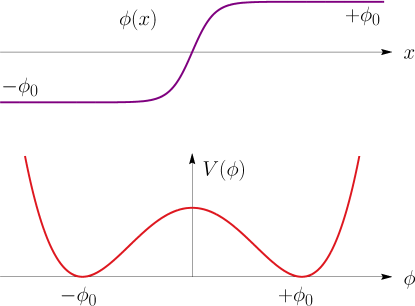
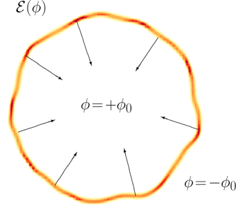
Figure 1.10: The left panel shows the potential energy (bottom), with a discrete degeneracy of the ground state: $\pm\phi_{0}$; and a typical one-dimensional domain-wall solution that interpolates between the two inequivalent ground states (top). The right panel displays a closed domain-wall, where the inner region is in one ground-state while the exterior falls into the other ground state. The closed domain-wall tends to collapse because of its line tension (the energy per unit-length $\cal E$).

The domain-walls, also referred to as kinks, thus appear in models where the ground state has a discrete degeneracy. The $\phi^{4}$-model is a textbook example of a theory that features domain-wall solutions (for detailed textbook discussion see e.g. [1, 4, 5, 3, 8]). As a reminder, this is a theory of a real scalar field with a quartic self-interacting potential $V(\phi)\propto(\phi^{2}-\phi_{0}^{2})^{2}$. As illustrated in Fig. 1.10, the ground state of this potential has a discrete degeneracy: $\pm\phi_{0}$. In one spatial dimension, the domain-walls feature topological protection and thus cannot transform into either of the ground-states. Indeed, the configurations that interpolate between $-\phi_{0}$ and $+\phi_{0}$ fall into disjoint homotopy classes, and thus no finite energy transformation can transform it to a constant ground state, see Fig. 1.10. In two dimensions, on the other hand, the Hobart-Derrick theorem implies that there are no static finite-energy solutions [143, 144]. Indeed, either the field asymptotically fall into degenerate ground states and in that case the domain-wall is infinitely long, or the domain-wall is closed with a finite length, but topological trivial. Thus closed domain-walls in two dimensions, being topologically trivial, do not enjoy any kind of topological protection. The energy of a closed domain-wall is finite and proportional to its length. Hence, as illustrated on the right panel of the Figure 1.10, since a closed domain-wall has no topological protection, it dynamically collapses due to its line tension (similarly to a vacuum bubble that shrinks because of its surface tension).

There exist various possibilities for a superconducting state to spontaneously break a discrete $\mathbb{Z}_{2}$ symmetry. One of them, is to break the time-reversal symmetry. The breakdown of the time-reversal symmetry typically occurs due to the competition between different phase-locking terms, between the different condensates. Aspects of time-reversal symmetry breaking in multicomponent superconductors, and especially the so-called ${s\!+\!is}$ state, are developed in details later in the Chapter 3. The details of the spontaneous breakdown of the time-reversal symmetry, may differ depending on the underlying properties of the model under consideration. For example, depending on whether the system is described by a two- or three-component Ginzburg-Landau theory, the terms responsible for the spontaneous breakdown of the time-reversal symmetry will be different (see the discussion in the Chapter 3). Considering again the scalar multiplet $\Psi$, the superconducting ground state is the field configuration $\Psi_{0}$ defined as $\Psi_{0}:=\mathrm{argmin}\,V(\Psi,\Psi^{\dagger})$. Heuristically, the time-reversal symmetry of the ground-state can be understood as the invariance $\Psi_{0}$ under complex conjugation (up to global $\mathrm{U}(1)$ transformations). Conversely, a superconducting state that spontaneously breaks the time-reversal symmetry satisfies the condition

$$\Psi_{0}^{*}\mathrm{e}^{i\chi}\neq\Psi_{0}\leavevmode\nobreak\ \leavevmode\nobreak\ \forall\chi\,.$$ (1.58)

Depending on the number of components, the difference between time-reversal symmetric (TRS) and broken time-reversal symmetry (BTRS) states, can be illustrated with the following simple examples (for normalized states $\Psi_{0}^{\dagger}\Psi_{0}=1$). For example, in the case of two components:

$$\Psi_{0} =(1,-1)/\sqrt{2} :\leavevmode\nobreak\ \leavevmode\nobreak\ \leavevmode\nobreak\ \,\Psi_{0}^{*} =(1,-1)/\sqrt{2}=\Psi_{0} \Longrightarrow\text{TRS\phantom{B}}$$

$$\Psi_{0}^{\pm} =(1,\pm i)/\sqrt{2} :\leavevmode\nobreak\ \Psi_{0}^{\pm*} =(1,\mp i)/\sqrt{2}=\Psi_{0}^{\mp}\neq\Psi_{0}^{\pm} \Longrightarrow\text{BTRS}\,.$$

Similarly, the case of three-components can be illustrated by:

$$\Psi_{0} =(1,1,-1)/\sqrt{3} :\leavevmode\nobreak\ \leavevmode\nobreak\ \leavevmode\nobreak\ \,\Psi_{0}^{*} =(1,1,-1)/\sqrt{3}=\Psi_{0} \Longrightarrow\text{TRS\phantom{B}}$$

$$\Psi_{0}^{\pm} =(1,\mathrm{e}^{\pm i\pi/3},\mathrm{e}^{\mp i\pi/3})/\sqrt{3} :\leavevmode\nobreak\ \Psi_{0}^{\pm*} =(1,\mathrm{e}^{\mp i\pi/3},\mathrm{e}^{\pm i\pi/3})/\sqrt{3}=\Psi_{0}^{\mp}\neq\Psi_{0}^{\pm} \Longrightarrow\text{BTRS}\,.$$

The superconducting states that break the time-reversal symmetry are thus not invariant under complex conjugation. More precisely, the time-reversal operations (the complex conjugation) sends one ground state onto the other. Symmetry-wise, in addition to the spontaneous breakdown of the $\mathrm{U}(1)$ gauge symmetry, the time-reversal symmetry breaking states also break the discrete $\mathbb{Z}_{2}$ symmetry associated with the complex conjugation. Using the above notations, $\Psi_{0}^{\pm}$ are thus two disconnected ground-states related to each other by the time-reversal operations $\Psi_{0}^{\pm*}=\Psi_{0}^{\mp}$. Hence the theory supports domain-walls as those illustrated in the Figure 1.10.

As discussed in more details in the Chapter 3, the frustrated competition between phase-locking terms in superconductors with two, three (or more) components yields ground states where the relative phases $\varphi_{ab}=\varphi_{b}-\varphi_{a}$ are neither $0$ nor $\pi$. Since it is not invariant under complex conjugation, such a ground-state spontaneously breaks the time-reversal symmetry [145, 146]. Indeed, for a two-component superconductor, the inter-component Josephson interaction $\propto|\psi_{a}||\psi_{b}|\cos\varphi_{ab}$ either locks or anti-locks the phases, so that the ground-state relative phase is respectively $0$ or $\pi$. With more than two components, each inter-component Josephson coupling favours (anti-)locking of the two corresponding phases. However, these Josephson terms can collectively compete so that optimal phases are neither locked nor anti-locked. Let consider here a simple potential for a three-component model with competing phase-locking terms

$$V=\sum_{a=1}^{3}\Bigg{\{}-|\psi_{a}|^{2}+\frac{1}{2}|\psi_{a}|^{4}+\sum_{b>a}^{3}|\psi_{a}||\psi_{b}|\cos\varphi_{ab}\Bigg{\}}\,.$$ (1.59)

The invariance under complex conjugation implies that, the potential energy does not change if the sign of all relative phases is changed, $\varphi_{ab}\to-\varphi_{ab}$. It follows that if any of the relative phases $\varphi_{ab}$ is not an integer multiple of $\pi$, then the ground state has an additional discrete $\mathbb{Z}_{2}$ degeneracy. This is the case of the potential (1.59) that admits two possible ground states: $\Psi_{0}^{+}$ with $\varphi_{12}=2\pi/3,\;\varphi_{13}=-2\pi/3$ or $\Psi_{0}^{-}$ with $\varphi_{12}=-2\pi/3,\;\varphi_{13}=2\pi/3$. This potential thus allows for domain-walls that interpolate between $\Psi_{0}^{+}$ and $\Psi_{0}^{-}$.

The domain-walls can typically form during cooling processes via the Kibble-Zurek mechanism [12, 13]. As mentioned previously, closed domain-walls in two spatial dimensions are unstable and collapse for dynamical reasons. Similarly domain-walls in finite domains decay for the same reasons. However, as demonstrated in [JG19.] they can be stabilized by geometric barrier in non-convex domains, or by the existence of pinning centres. Such a mechanism for the geometric stabilization of domain walls, illustrated in Fig. 1.11, may help for their observability. If during a quench a domain-wall ending on the short (non-convex) parts of the domain, is created via the Kibble-Zurek mechanism, it can relax to a (meta)stable configuration. Indeed, for both ends of the domain-wall to join and then collapse to zero size, the domain-wall would have to first increase its length. Unlike the domain-walls in chiral $p$-wave superconductors, that carry a uniform magnetic field orbital momentum of Cooper pairs (see e.g. [147, 148, 149]), domain-walls between ${s\!+\!is}$ states carry a magnetic field only locally [JG19.]. Namely it features opposite local field at its ends, with a total net flux through the sample that is zero.

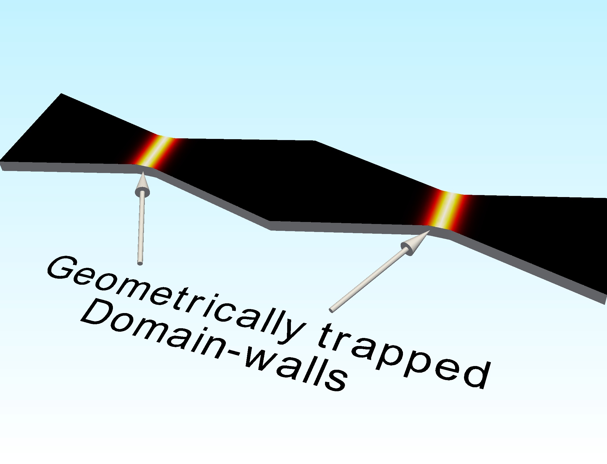
Figure 1.11: This sketches the principle of the geometric stabilization of domain-walls in non-convex domains [JG19.]. The domain-walls, for example formed via the Kibble-Zurek mechanism in a rapid quench, are geometrically trapped. Indeed, for a domain-wall to escape it should increases its length, which is energetically costly.

along the walls

The fractional vortices are confined together, due to the energy cost associated with the neutral sector. Note that since the phase-locking terms in (1.59) provide a potential energy for the relative phases, the attraction here is linear and not logarithmic as derived in (1.33). A domain-wall interpolating between two time-reversal symmetry broken states is, by definition the region where the phase-locking is the least optimal. As a result, it allows to accommodate a more favourable relative phase by splitting the integer flux singular vortices into fractional flux vortices. Moreover since the superfluid density is suppressed on a domain-wall, because of the field gradients, it can pin vortices. Thus while in the bulk, the fractional vortices are confined because of the strong linear attractive interaction, they repel each other when bound to a domain-wall (see detailed discussion in [142, 120, 119], and later in Section 3.2.2). This implies that the magnetization processes can be strongly altered if a system has some pre-existing domain-walls that are geometrically trapped [JG19.]. Indeed, since some density components are depleted at the domain wall, the vortex entry for the corresponding component costs much less energy there, than from other parts of the boundaries. It follows that the first vortex entry can occur at lower fields than $H_{c1}$, since they have to overcome a smaller Bean-Livingston barrier on the domain-wall than in the bulk.

The interaction between fractional vortices confined on the domain-walls between different time-reversal symmetry broken ${s\!+\!is}$ states is repulsive. On the other hand, closed (bare) domain-walls, as sketched in Fig. 1.10, collapse due to their line tension. This thus hints to a scenario where both tendency would compromise, leading to an object with a closed domain-wall of finite size, stabilized by the repulsion between confined fractional vortices. As demonstrated in [JG26.] and [JG21.], such composite objects can indeed be formed either as metastable states, or as thermodynamically stable excitations, in external fields. Moreover, as these flux carrying topological defects consist in non-overlapping fractional vortices, they carry a quantized $\mathbb{C}\mathrm{P}^{2}$ topological invariant (1.17). These composite objects, that are bound states of domain-walls and fractional vortices are called chiral $\mathbb{C}\mathrm{P}^{2}$ skyrmions. The prefix chiral refers to the fact that the fractional vortices order differently along the wall, in the different time-reversal symmetry broken states [JG21.].

The chiral $\mathbb{C}\mathrm{P}^{2}$ skyrmions can be formed via various scenario, as for example during field-cooled quenches in external fields [119]. Since the have very specific magnetic signatures, they may be observed (and easily discriminated from singular vortices) for example in high-resolution scanning SQUID, Hall, or magnetic force microscopy measurements [142, 120].

1.3.4 Skyrmions stabilized by condensate repulsion

It was previously emphasized that the existence of skyrmions requires a stabilizing mechanism to counteract the predisposition of the singularities to superimpose. Some of the mechanisms presented above can split the vortex cores, even in the London limit. This is for example the case of condensates with commensurate charges in Sec. 1.3.1, or with dissipationless drag introduced in Sec. 1.3.2. The core-splitting mechanism is still effective beyond the London limit. Roughly speaking, these mechanisms for core splitting rely on modifications on the kinetic terms. On the other hand, the mechanism that splits the fractional vortices confined on a domain-wall, introduced in Sec. 1.3.3, has no counterpart in the London limit. The stabilization of the chiral $\mathbb{C}\mathrm{P}^{2}$ skyrmions is thus purely a nonlinear effect. This section, presents another mechanism which is also purely nonlinear, and that originates only in the potential terms; namely the bi-quadratic inter-component coupling. This interaction which impedes the coexistence of the condensates is relevant for a broad variety of models.

Using the generic structure of the potential term (1), the bi-quadratic interactions are the terms which are quadratic in two of the individual densities. Namely they read as

$$\cdots+\sum_{a,b>a}\beta_{ab}|\psi_{a}|^{2}|\psi_{b}|^{2}+\cdots\,,$$ (1.60)

where the coefficients correspond to $\beta_{ab}:=\beta_{abab}$ in (1). Depending on the sign of the bi-quadratic coupling $\beta_{ab}$, this interaction either promotes ($\beta_{ab}<0$) or impedes ($\beta_{ab}>0$) the coexistence of both condensates densities $|\psi_{a}|^{2}$ and $|\psi_{b}|^{2}$. For example, if the bi-quadratic interaction is repulsive ($\beta_{ab}>0$) and strong, it can promote a phase separation where one of the condensate vanishes in the ground state (for example $|\psi_{a}|\neq 0$ and $|\psi_{b}|=0$). These terms not only modify the ground state properties, but also alter the interactions between the elementary topological defects. Indeed, the repulsive bi-quadratic interaction (when $\beta_{ab}>0$) typically promotes core splitting of the composite vortices. That is, it enforces the situation where the singularities of the ensuing fractional vortices do not overlap. This kind of inter-component interactions obviously cannot be accounted by the the London limit, where densities are constant.

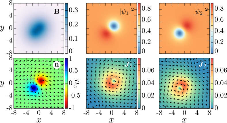
Figure 1.12: A skyrmion solution of a two-component superconductor, stabilized by the repulsive bi-quadratic interaction (1.60). The parameters of the later detailed potential (2.12) are $(\alpha_{aa},\beta_{aa})=(-1,1)$, $\beta_{12}>0$ and the gauge coupling is $e=0.25$. The displayed quantity on the top left panel is the magnetic field. The other panels on the top row, show the individual densities of the superconducting condensates $|\psi_{1}|^{2}$ and $|\psi_{2}|^{2}$. The bottom left panel shows the associated pseudo-spin texture $\bm{n}$ (1.37), while the other panels on the bottom row, are the individual currents ${\bm{J}}_{a}$.

As illustrated in the Figure 1.12, the bi-quadratic interaction indeed can favour core splitting. It is clear from the panels showing the individual densities that the solution feature non-overlapping vortices in both components, thus implying that the vortex is coreless. It follows that again it is characterized by the additional invariant $\mathcal{Q}(\Psi)=1$ (1.17). The skyrmion here consists of one meron and an anti-meron of the pseudo-spin texture $\bm{n}$ (1.37). Again these stand for the fractional vortices in the individual components, similarly to Fig. 1.4.

These skymrions have a magnetic field that is not axially symmetric, and thus may be detectable by local magnetic field measurement, such as scanning SQUID. Furthermore, similarly to the skyrmions stabilized by the Andreev-Bashkin term in Sec. 1.3.2, the relative phase exhibits a dipolar mode that is long-ranged. These skyrmions thus interact non trivially together.

As already mentioned, the bi-quadratic interaction (1.60) in the phenomenological Ginzburg-Landau models, may occur in a broad variety of contexts describing different microscopic physics. Below, is a brief overview of the different microscopic systems which yield a bi-quadratic interaction that stabilizes skyrmions.

Skyrmions in interface superconductors.

Superconductors with strong Rashba spin-orbit coupling can exhibit skyrmions similar to that displayed in Fig. 1.12. More precisely, in a weak-coupling theory for a clean superconductor with isotropic pairing interactions ($s$-wave pairing), an in-plane Zeeman field, and a strong Rashba spin-orbit coupling, the resulting Ginzburg-Landau theory features bi-quadratic interaction (1.60). As discussed in details in [JG17.], this applies for example to interface superconductors, such as SrTiO₃/LaAlO₃.

Skyrmions in immiscible mixtures of two condensates.

The bi-quadratic interactions can also be responsible for the spontaneous breakdown of a discrete $\mathbb{Z}_{2}$ symmetry, different than the competition between phase-locking terms discussed in Sec. 1.3.3. For example, if a global $\mathrm{SU}(2)$ symmetry is explicitly broken by bi-quadratic interactions (1.60). Namely, for a potential term $V=\Lambda(\Psi^{\dagger}\Psi-\Psi_{0}^{2})^{2}+\delta|\psi_{1}|^{2}|\psi_{2}|^{2}$. There the global $\mathrm{SU}(2)$ symmetry of the potential is explicitly broken down to $\mathrm{U}(1)\!\times\!\mathrm{U}(1)\!\times\!\mathbb{Z}_{2}$. If the symmetry breaking parameter $\delta>0$, then the condensates cannot coexist and the ground state is either $(\Psi_{0},0)$ and $(0,\Psi_{0})$. This thus describes an immiscible mixture of two condensates. As a result the theory also supports domain-walls which can combine to the vorticity and result into skyrmions [JG16.]. This is easily understood that when one of the component is suppressed (e.g. at a vortex core), then it is beneficial to condense the other component there. They can form giant skyrmions carrying several flux quanta even in a type-2 regime. As discussed [JG16.] and [JG15.], this strongly affect the magnetization properties.

Skyrmions in nematic superconductors

The Ginzburg-Landau theory that describes some odd-parity nematic superconductors feature skyrmions similar to that displayed Fig. 1.12. As argued in [JG7.], Cu_xBi₂Se₃ is a candidate material for the existence of such skyrmions. Note however that the appropriate Ginzburg-Landau theory to describing such nematic superconductors, also features additional kinetic terms that are anisotropic and mix the different components. These extra terms read as [JG7.]

$$\kappa_{1}\mathrm{Re}\left[(D_{x}\psi_{1})^{*}D_{x}\psi_{2}-(D_{y}\psi_{1})^{*}D_{y}\psi_{2}\right]+\kappa_{2}\mathrm{Im}\left[(D_{x}\psi_{1})^{*}D_{y}\psi_{2}+(D_{y}\psi_{1})^{*}D_{x}\psi_{2}\right]\,.$$ (1.61)

Such term definitely alter the structure of the skyrmions, and their interactions. However, this is again the bi-quadratic interaction that is the principal ingredient of the vortex splitting.

Skyrmions in chiral $p$-wave superconductors

Chiral $p$-wave superconductors also feature bi-quadratic interaction that promotes core splitting. Like for the nematic superconductors, they also feature additional kinetic terms of the form (1.61). As demonstrated in [JG23.], the Ginzburg-Landau models for ${p\!+\!ip}$ superconductors, do support skyrmion excitation. Depending on the regions of the parameter space they can be energetically favoured as compared to singular vortices. In particular, it was demonstrated that charge-2 skyrmions can be interpreted as two-quanta vortices, and that they are always preferred over isolated single quanta vortices [JG13.]. Lattices of these two-quanta vortices form spontaneously in an external magnetic field. In high applied field, the lattice of two-quanta vortices dissociates into a lattice of single quantum vortices [JG11.], and this picture persists beyond the mean field approximation [JG3.].

Chapter 2 Type-1.5 superconductivity

Superconductors with multicomponent order parameters, not only allow for a rich zoology of topological defects that have no counterpart in single-component systems (fractional vortices, skyrmions, hopfions, etc), but they also allow for richer kind of interactions between them. As introduced in the previous chapter, the elementary topological excitations in multicomponent superconductors are vortices carrying a fraction of the flux quantum. These combine to form composite defects (either singular or coreless) so that, in the bulk, the only finite-energy excitations carry an integer flux. Regardless of their core structure, the interactions between the topological defects are ruled, to a large extent, by the characteristic length-scales of the theory (or equivalently the mass spectrum). Single-component superconducting condensates are characterized by a the coherence length $\xi$ associated with the density variations (Anderson-Higgs mode). Multicomponent order parameters, on the other hand, typically feature several length-scales. While the associated scalar modes are typically attractive, the charged modes, associated with penetration depth $\lambda$ of the gauge field, mediate repulsion between flux carrying defects. See the discussion about single-component superconductors in the Appendix A.

The textbook classification divides superconductors into two classes, depending on their behaviour in an external field. This classification is quantified by the dimensionless Ginzburg-Landau parameter $\kappa$ defined as the ratio of both fundamental length-scales $\kappa=\lambda/\xi$. When $\sqrt{2}\lambda<\xi$ (type-1), superconductors expel low magnetic field (the Meissner state), while macroscopic normal domains are formed when large fields are applied [150, 73]. On the other hand type-2 superconductors, for which $\xi<\sqrt{2}\lambda$, feature thermodynamically stable vortex excitations [151]. More precisely, the magnetic field is expelled below some critical value $H_{c1}$. Above this value, and until the destruction of superconductivity at the second critical field $H_{c2}$, type-2 superconductors form lattices or liquids of vortices carrying a flux quantum. These behaviour are summarized in Fig. 2.1 and in tables 2.1 and 2.2. The energy cost of a boundary between normal and superconducting states is positive in the type-1 regime. The absence of thermodynamically stable vortices, and the formation of macroscopic normal domains, thus follows from the minimization of the interface energy. It results that intervortex forces are purely attractive (thus vortices collapse to a giant vortex). On the other hand, type-2 superconductors support thermodynamically stable single-quanta vortices, as the boundary energy between normal and superconducting states is negative. The interaction between vortices is purely repulsive, and they form (triangular) Abrikosov lattices [151]. In the Ginzburg-Landau theory, at the critical value $\kappa=1/\sqrt{2}$ (called the Bogomol’nyi point), vortices do not interact [152, 153]. There, the current-current repulsion exactly compensates the core-core attraction at all distances.

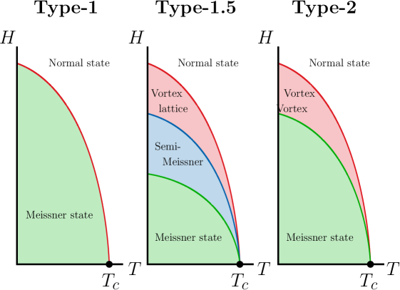
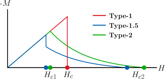
Figure 2.1: Phase diagrams of superconductors in type-1, type-2 and type-1.5 regimes.

Unlike in single-component superconductors, it is not possible to construct a single dimensionless parameter for multicomponent superconductors featuring several coherence lengths $\xi_{a}$. Hence the usual type-1/type-2 dichotomy is insufficient to capture the whole physics, and to classify multicomponent superconductors. Indeed, since the coherence lengths $\xi_{a}$ associated with the superconducting condensates are typically different, the penetration depth $\lambda$ can formally be an intermediate length-scale: $\xi_{1}\!<\!\cdots\!<\!\sqrt{2}\lambda\!<\!\cdots\!<\!\xi_{N}$. For such a length-scale hierarchy, the modes associated with the length-scales larger than $\sqrt{2}\lambda$ provide long-range attraction as in type-1 superconductors. On the other hand, the modes with length-scales shorter than $\sqrt{2}\lambda$ enable short-range repulsion, as in the type-2.

Consider, for example, a two-component superconductor satisfying this length-scale hierarchy: $\xi_{1}<\sqrt{2}\lambda<\xi_{2}$. There, the mode associated with the largest length-scale $\xi_{2}$ should provide a long-range intervortex attraction (loosely speaking due to the “outer cores" overlap). On the other hand, the current-current and electromagnetic interaction associated with $\lambda$ provides a short-range repulsive interaction. The competition between these behaviours opens the possibility of a non-monotonic intervortex interacting potential that is long-range attractive (as in type-1 regime) and short-range repulsive (as in type-2 regime). This compromise between the type-1 and type-2 behaviours motivated the type-1.5 terminology of such states [154]. The hierarchy where $\lambda$ is an intermediate length-scale is a necessary, although not sufficient condition, to realize non-monotonic intervortex interactions. Yet, if realized, the non-monotonic forces result in a preferred intervortex distance such that two vortices form a bound state, and that many vortices coalesce to form vortex aggregate (clusters), coexisting with macroscopic domains of Meissner (vortexless) state: the semi-Meissner state [155].

	Characteristic lengths-scales	Intervortex interaction	Energy of $N$-quantum vortex
Single-component type-1	Penetration length $\lambda$ and coherence length $\xi$, with $\lambda/\xi<1/\sqrt{2}$	Attractive	$\frac{E(N)}{N}<\frac{E(N-1)}{N-1}$. Vortices collapse onto an $N$-quantum single mega-vortex.
Single-component type-2	Penetration length $\lambda$ and coherence length $\xi$, with $\lambda/\xi>1/\sqrt{2}$	Repulsive	$\frac{E(N)}{N}>\frac{E(N-1)}{N-1}$. $N$-quantum vortex decays into $N$ infinitely separated single-quantum vortices
Multicomponent type-1.5	Multiple length scales $\xi_{a}$, and the penetration length $\lambda$. Non-monotonic vortex interaction occurs when $\xi_{1}\leq\cdots<\sqrt{2}\lambda\leq\cdots\leq\xi_{N}$	Non-monotonic: long-range attractive and short-range repulsive	$N$-quantum vortices decay into vortex clusters. Isolated single-quantum vortices attract to form a cluster

Table 2.1: Characteristics of bulk clean superconductors in the type-1, type-2 and type-1.5 regimes. Here the most common units are used in which the value of the Ginzburg-Landau parameter $\kappa$ which separates type-1 and type-2 regimes in a single-component theory is $\kappa_{c}=1/\sqrt{2}$.

	Superconducting/normal state interface energy	Magnetic field required to form a vortex	Phases in an external magnetic field
Single-component type-1	Positive	Larger than the thermodynamical critical magnetic field	(i) Meissner state at low fields; (ii) Macroscopically large normal domains at elevated fields. First order phase transition Meissner$\to$Normal
Single-component type-2	Negative	Smaller than the thermodynamical critical magnetic field	(i) Meissner state at low fields, (ii) Vortex lattices/liquids at larger fields. Second order phase transitions: Meissner$\to$Vortex and Vortex$\to$Normal (at the level of mean-field theory).
multicomponent type-1.5	Negative SC/N interface energy inside vortex clusters but positive energy of the cluster’s boundary	Either: (i) smaller than the thermodynamical critical magnetic field or (ii) larger than critical magnetic field for single vortex but smaller than critical magnetic field for a vortex cluster of a certain critical size	(i) Meissner state at low fields, (ii) Macroscopic phase separation into vortex clusters coexisting with Meissner domains at intermediate fields (iii) Vortex lattices/liquids at larger fields. Vortices form via a first order phase transition. The transition from vortex states to normal state is second order.

Table 2.2: Continued characteristics of the type-1, type-2 and type-1.5 regimes. The corresponding magnetization curves in these regimes are displayed on Fig. 2.1.

The magnetic response of single-component superconductors can be classified by considering interface energy between the superconducting and the normal state (see details in Appendix A). In the type-1.5 regime of multicomponent systems, such an argument cannot be straightforwardly applied. Indeed, the energy per vortex greatly depends on whether or not the vortex is located inside a cluster. Indeed, inside a cluster (where the vortices are placed in a minimum of the interaction potential), the energy per flux quantum is smaller than that for an isolated vortex. Hence, the formation of a single isolated vortex might be energetically unfavourable, while the formation of vortex clusters can be favourable. Moreover, besides the energy of the vortices inside the clusters, there appears additional characteristics associated with the energy of the boundary of the cluster itself. In other words systems with inhomogeneous vortex states are characterized by several different interfaces, some of which having positive and some with negative free energy. Overall, this is the non-monotonic intervortex interaction which defines the essential properties of the type-1.5 regime, but this is not a state-defining one. Indeed, the attraction between vortices can arise under certain circumstances in single-component materials as well. However, in the case of the type-1.5 regime, the long-range attraction is a consequence of multiple coherence lengths and comes with several new physical effects discussed below.

The previous chapter introduced the generic framework of multicomponent systems, and of their topological properties. There was a particular focus on the various interactions that can result in coreless topological defect. Here the central point is about singular defects where the core of constituting individual vortices overlap.

Plan of the Chapter

As stated in the introduction of this chapter, the essential ingredient for the type-1.5 regime in multicomponent superconductors, is to have a hierarchy such that the penetration depth is an intermediate length-scale. Thus, as a starting point, the Section 2.1 will present the general framework for the analysis of the length-scales. This follows from the analysis of the eigenspectrum of the (linear) perturbation operator around the ground state. The general framework is then supplemented with a particular example that can be addressed analytically.

The length-scales, defined from the eigenspectrum of the perturbation operator, determine the asymptotic behaviour of vortex matter. In particular, as detailed in the Section 2.1.3, this controls the long-range interaction between vortices [156]. If the penetration depth is an intermediate length-scale, then the intervortex forces are long-range attractive and short-range repulsive. This strongly suggests that vortices should form bound states with a preferred separation.

When the length-scale hierarchy allows for non-monotonic intervortex forces, then vortices can aggregate together thus forming vortex clusters surrounded by vortex-less regions of Meissner state. Few examples of such clusters are exemplified in Section 2.2.

Next, the Section 2.3 examines the possible mechanism that should lead to the formation of vortex clusters; and the various models where this was observed. The possible experimental signatures of the vortex clusters, and their relevance are presented there as well.

Summary of the results that are relevant for this chapter

• Finding of a new kind of multibody intervortex forces in multiband superconductors [JG27.]. The non-monotonic intervortex interactions lead to the formation of vortex clusters surrounded by macroscopic Meissner domains (vortexless state). The structure formation can be highly impacted by non-pairwise intervortex interactions, originating in the nonlinear superposition of vortices. The non-monotonic intervortex forces also result in cluster formation in three-band superconductors [JG25.]. See reviews in [JG24.]. Non-monotonic intervortex forces can also occur in superconducting systems with competing order parameters. That is when the intercomponent interactions prohibit the coexistence of two condensates in the ground state [JG16.] and [JG15.].

• Explanation of the vortex coalescence in an putative two-band model for Sr₂RuO₄ superconducting material [JG22.]. We argued that the observed vortex coalescence in Sr₂RuO₄ can be explained by non-monotonic interactions originating in the multiband nature of Sr₂RuO₄ . Vortex coalescence in Sr₂RuO₄ received experimental support from $\mu$SR measurements in Phys. Rev. B 89, 094504 (2014) [157].

• Prediction of an unconventional magnetic response in interface superconductors with a strong Rashba spin-orbit coupling [JG17.]. We demonstrate microscopically that in the clean limit interface superconductors, such as SrTiO₃/LaAlO₃, can exhibit formation of vortex clusters.

• In a series of works on the microscopic properties of dirty two-band superconductors, we demonstrated that they feature regions of the parameter space, where the hierarchy of length-scales allows in principle the formation of vortex clusters due to the vicinity of an hidden second order phase transition within the superconducting state [JG9.]. This should similarly occur in clean three-band systems [JG10.]. Numerical simulations show that it indeed occurs, and that this results in peculiar signals that can be discriminated from other scenarios via global measurements of the response of muon-spin-rotation experiments [JG5.].

2.1 Length-scales in multicomponent systems

The possibility that the interaction between vortices in multicomponent systems can be non-monotonic relies on the non-trivial hierarchy of the length-scales of the theory. It is also based on the asymptotic interaction between vortices already introduced in the previous section 1.1.4. Before reviewing the intervortex interactions in the context of the semi-Meissner state, we review below the general framework, and the analysis of the length-scales of multicomponent Ginzburg-Landau theory.

To illustrate the underlying mechanism for the semi-Meissner state, let consider here a restriction of the generic free energy (1), for $N$ superconducting condensates coupled via various intercomponent interactions

$$\mathcal{F}/\mathcal{F}_{0} =\bigintsss\frac{1}{2}\big{|}{\bm{\nabla}}\!\times\!{\bm{A}}\big{|}^{2}+\sum_{a=1}^{N}\frac{1}{2}\big{|}{\bm{D}}\psi_{a}\big{|}^{2}+V(\Psi,\Psi^{\dagger})\,,$$ (2.1a)

$$\text{where}\leavevmode\nobreak\ V(\Psi,\Psi^{\dagger}) =\sum_{a=1}^{N}\left(\alpha_{aa}|\psi_{a}|^{2}+\frac{1}{2}\beta_{aa}|\psi_{a}|^{4}\right)+\sum_{a=1}^{N}\,\sum_{b>a}^{N}\alpha_{ab}\big{(}\psi_{a}^{*}\psi_{b}+\psi_{b}^{*}\psi_{a}\big{)}$$ (2.1b)

$$+\sum_{a=1}^{N}\,\sum_{b>a}^{N}\beta_{ab}|\psi_{a}|^{2}|\psi_{b}|^{2}+\sum_{a=1}^{N}\,\sum_{b>a}^{N}\frac{\gamma_{ab}}{2}\big{(}\psi_{a}^{*2}\psi_{b}^{2}+\psi_{b}^{*2}\psi_{a}^{2}\big{)}\,.$$ (2.1c)

For simplicity again, we consider the absence of mixed gradient terms (namely $\kappa_{ab}=\delta_{ab}$). The role of mixed gradient terms , in the context of the semi-Meissner state, was discussed in details in [158]. Also the possibility to eliminate mixed gradient terms in two-component systems was discussed in [159, 160]. The role of mixed gradients, and the possibility for anisotropies was also considered, see [161] and [162] for extensions to chiral $p$-wave superconductivity. In principle other interaction terms are allowed on symmetry grounds, but the potential (2.1c) is general enough for the current discussion. The ground state values of the fields $|\psi_{a}|$ and $\varphi_{ab}$ of free energy (2.1) are found by minimizing its potential energy:

$$\Psi_{0}=\underset{\Psi\in\mathbbm{C}^{N}}{\mathrm{argmin}}\leavevmode\nobreak\ V(\Psi,\Psi^{\dagger})\,.$$ (2.2)

The ground state is determined by the system of equations given by the variations of the potential, with respect to the physical degrees of freedom $|\psi_{a}|$ and $\varphi_{a}$.

2.1.1 Length-scales

The length-scales that characterize the superconducting degrees of freedom are called the coherence lengths, while that associated with the gauge field is the London penetration depth. These length-scales are the exponents that characterise how the ground state is recovered from an infinitesimal perturbation. The analysis of the length-scales, or equivalently of the mass spectrum, of the theory is achieved by investigating the linear response to infinitesimally small perturbation

$$\psi_{a}=(u_{a}+\epsilon f_{a})\exp\left\{i\left({\bar{\varphi}}_{a}+\epsilon\frac{\phi_{a}}{u_{a}}\right)\right\}\,,\leavevmode\nobreak\ \leavevmode\nobreak\ \leavevmode\nobreak\ \text{and}\leavevmode\nobreak\ \leavevmode\nobreak\ {\bm{A}}=\epsilon{\bm{a}}\,.$$ (2.3)

Here, $u_{a}$ and ${\bar{\varphi}}_{a}$ are respectively the ground state densities and phases introduced in the previous section. $f_{a}\equiv f_{a}(\mathbf{x})$ are the density amplitudes, while $\phi_{a}\equiv\phi_{a}(\mathbf{x})$ are the normalized phase amplitudes. The amplitudes ${\bm{a}}\equiv{\bm{a}}(\mathbf{x})$ characterize the fluctuations of the gauge field around the ground state.

Inserting the expansion (2.3) inside the free energy (2.1), and collecting order by order in $\epsilon$ determines the fluctuation operator. More precisely, the zeroth order in $\epsilon$ defines the energy of the ground state, and the first order in $\epsilon$ determines by the ground state. The quadratic term in $\epsilon$ defines the perturbation operator whose eigenvalues determine the mass spectrum of the theory. The fluctuations are characterized by a system of Klein-Gordon equations for the $2N$ condensate fluctuations ($N$ densities plus $N$ phases), plus one Proca equation for the gauge field. In the gauge where ${\bm{\nabla}}\!\cdot\!{\bm{a}}=0$, the fluctuation operator reads as

$$\frac{1}{2}\Upsilon^{T}\left(-{\bm{\nabla}}^{2}+{\cal M}^{2}\right)\Upsilon\,,\leavevmode\nobreak\ \leavevmode\nobreak\ \leavevmode\nobreak\ \text{where}\leavevmode\nobreak\ \leavevmode\nobreak\ \leavevmode\nobreak\ \Upsilon=(f_{1},\cdots,f_{N},\phi_{1},\cdots,\phi_{N},{\bm{a}})^{T}\,.$$ (2.4)

Here ${\cal M}^{2}$ is the (squared) mass matrix that can be read from

$$\Upsilon^{T}{\cal M}^{2}\Upsilon=e^{2}\sum_{a=1}^{N}u_{a}^{2}{\bm{a}}^{2}+\sum_{a=1}^{N}2(\alpha_{aa}+3\beta_{aa}u_{a}^{2})f_{a}^{2}+\sum_{a=1}^{N}\sum_{b>a}^{N}2\alpha_{ab}f_{a}f_{b}\cos{\bar{\varphi}}_{ab}$$ (2.5a)

$$+\sum_{a=1}^{N}\sum_{b>a}^{N}\frac{2\alpha_{ab}}{u_{a}u_{b}}\Big{\{}(u_{a}f_{b}+f_{b}u_{a})\big{(}\phi_{b}u_{a}-\phi_{a}u_{b}\big{)}\sin{\bar{\varphi}}_{ab}-\frac{1}{2}\big{(}\phi_{b}u_{a}-\phi_{a}u_{b}\big{)}^{2}\cos{\bar{\varphi}}_{ab}\Big{\}}$$ (2.5b)

$$+\sum_{a=1}^{N}\sum_{b>a}^{N}2\big{(}\beta_{ab}+\gamma_{ab}\cos 2{\bar{\varphi}}_{ab}\big{)}\big{(}u_{a}^{2}f_{b}^{2}+4u_{a}u_{b}f_{a}f_{b}+u_{b}^{2}f_{a}^{2}\big{)}$$ (2.5c)

$$-\sum_{a=1}^{N}\sum_{b>a}^{N}4\gamma_{ab}\Big{\{}\big{(}u_{b}\phi_{a}-u_{a}\phi_{b}\big{)}^{2}\cos 2{\bar{\varphi}}_{ab}+2(u_{a}f_{b}+f_{b}u_{a})\big{(}\phi_{b}u_{a}-\phi_{a}u_{b}\big{)}\sin 2{\bar{\varphi}}_{ab}\Big{\}}\,.$$ (2.5d)

The eigenspectrum of the matrix ${\cal M}^{2}$ determines the squared masses of the excitations and the corresponding normal modes. The inverse of each mass $m_{a}$ defines a characteristic length-scale $\ell_{a}:=1/m_{a}$ of the theory. Note that the eigenspectrum of ${\cal M}^{2}$ always contains a zero mode, which is associated to the Goldstone boson that gives the mass to the gauge field.

Remark that there are alternative possibilities to investigate the length-scale spectrum of the theory. For example, by inserting a perturbative expansion in terms of the gauge invariant physical fields inside the free energy (1.12), expressed in terms of charged and neutral modes. Such an approach is explained in details in the Section A.1 of the Appendix A, in the case of single-component Ginzburg-Landau theory.

Penetration depth:

Clearly, the gauge field fluctuations always decouple from the fluctuations associated with the superconducting state. The (squared) mass of the gauge field is given by the total density as $m_{\bm{A}}=e^{2}\sum_{a=1}^{N}u_{a}^{2}$. The associated length-scale, the penetration depth is thus $\lambda=1/e\sqrt{\sum_{a=1}^{N}u_{a}^{2}}$. It is important to note that, given a ground state, the penetration depth can be adjusted to any value by tuning the gauge coupling $e$.

Length-scale hierarchy:

It is important to stress that the modes associated to the superconducting fluctuations are in general all coupled together. This means that, the matrix ${\cal M}^{2}$ is in general a dense, symmetric, square matrix. Unless ${\cal M}^{2}$ is a multiple of the identity, the mass spectrum cannot be fully degenerate. This implies that there is a hierarchy of the eigenmasses:

$$m_{0}=0\leq m_{I}\leq m_{II}\leq\cdots\leq m_{2N-1}\,,$$ (2.6)

and at least one the inequality is a strict inequality. The first mass $m_{0}=0$ is the Goldstone zero mode associated with the global symmetry mentioned above. It follows that there is a hierarchy of the physical length-scales

$$\ell_{I}\geq\ell_{II}\geq\cdots\geq\ell_{2N-1}\,,$$ (2.7)

where at least one the inequality is a strict inequality. Note that in certain situations, because of the underlying symmetry, the mass matrix can become block-diagonal. This is for example the case which is discussed below. The underlying symmetry is thus associated with a zero mode, but this does not change the fact that, in general, the mass spectrum is non-degenerate.

Now, taking the penetration depth into account, there are only three possible hierarchies of the length-scales :

• all the coherence lengths are larger than $\lambda$ (which is a type-1 behaviour)

• all the coherence lengths are smaller than $\lambda$ (which is a type-2 behaviour)

• the penetration depth $\lambda$ is an intermediate length-scale (the so-called “type-1.5" regime [154])

Since the penetration depth can be adjusted to any value by tuning the gauge coupling $e$, the hierarchy (2.7) implies that for any set of parameters of the theory, it is possible to find a value of $e$ such that $\lambda$ is an intermediate length-scale

$$\ell_{I}\geq\cdots\geq\lambda\geq\cdots\geq\ell_{2N-1}\,.$$ (2.8)

Of course, this does not imply that such choice of parameter is realized in the nature. The physical realizability of the length-scale hierarchy (2.8) is discussed later. The discussion of the hierarchy of length-scales can further be extend to anisotropic models [161]. As discussed below, since the intervortex interactions are related to the long-range asymptotics, such a hierarchy of the length-scales suggests long-range attractive, short-range repulsive intervortex forces.

Remark that the eigenmasses $m_{a}$, or equivalently the length-scales $\ell_{a}$, can be used to determine the coherence lengths $\xi_{a}=\sqrt{2}/m_{a}=\sqrt{2}\ell_{a}$. The factor $\sqrt{2}$ factor in the definition of coherence length is a matter of convention. This convention is that where the non-interacting regime (the Bogomol’nyi regime [153]) is $\kappa=1/\sqrt{2}$ for single-component superconductors [163], see Appendix A. The length-scale hierarchy (2.8) thus becomes:

$$\xi_{I}\geq\cdots\geq\sqrt{2}\lambda\geq\cdots\geq\xi_{2N-1}\,.$$ (2.9)

Coherence lengths:

The expression of the mass matrix (2.5) is very generic, and not all aspects are relevant for the present discussion. In particular, depending on the properties of the ground state, the perturbation operator can greatly simplify. There exist two-qualitatively different ground states: Ground states with trivial phase-locking, i.e. ${\bar{\varphi}}_{ab}=0,\pi$, and ground state with non-trivial relative phases ${\bar{\varphi}}_{ab}\neq 0,\pi$. The later case features new properties, and will be discussed in more details later in the Chapter 3 about the superconducting states that break the time-reversal symmetry. So, let focus here on the case of trivial phase-locking, where the ground state relative phases are ${\bar{\varphi}}_{ab}=0,\pi$. There, since $\sin{\bar{\varphi}}_{ab}=0$, the normalized phase amplitudes $\phi_{a}$ decouple from the density amplitudes $f_{a}$.

The mass of the density amplitudes $f_{a}$ are thus given by the eigenvalues of ${\cal M}_{ff}^{2}$ defined from

$$\Upsilon_{f}^{T}{\cal M}_{ff}^{2}\Upsilon_{f}=\sum_{a=1}^{N}2(\alpha_{aa}+3\beta_{aa}u_{a}^{2})f_{a}^{2}+\sum_{a=1}^{N}\sum_{b>a}^{N}2\alpha_{ab}f_{a}f_{b}\cos{\bar{\varphi}}_{ab}$$ (2.10a)

$$+\sum_{a=1}^{N}\sum_{b>a}^{N}2\big{(}\beta_{ab}+\gamma_{ab}\cos 2{\bar{\varphi}}_{ab}\big{)}\big{(}u_{a}^{2}f_{b}^{2}+4u_{a}u_{b}f_{a}f_{b}+u_{b}^{2}f_{a}^{2}\big{)}\,.$$ (2.10b)

Hence, as long as $\alpha_{ab}\neq 0$, or $\beta_{ab}\neq 0$, or $\gamma_{ab}\neq 0$, the density modes are in general mixed. It follows that the characteristic length-scales of the density fields are associated with the linear combinations of the fields, see e.g. [164, 158, 165]. Physically this implies that disturbing one of the density fields necessarily perturbs the others. This also implies that in a vortex, the long-range asymptotics of all density fields is governed by the same exponent, corresponding to a mixed mode with the smallest mass.

The masses of the normalized phase amplitudes $\phi_{a}$, on the other hand are given by the eigenvalues of ${\cal M}_{\phi\phi}^{2}$ defined from

$$\Upsilon_{\phi}^{T}{\cal M}_{\phi\phi}^{2}\Upsilon_{\phi} =-\sum_{a=1}^{N}\sum_{b>a}^{N}\Big{(}\frac{\alpha_{ab}}{u_{a}u_{b}}\cos{\bar{\varphi}}_{ab}+4\gamma_{ab}\cos 2{\bar{\varphi}}_{ab}\Big{)}\big{(}u_{b}\phi_{a}-u_{a}\phi_{b}\big{)}^{2}$$ (2.11a)

$$=-\sum_{a=1}^{N}\sum_{b>a}^{N}\Big{(}\alpha_{ab}u_{a}u_{b}\cos{\bar{\varphi}}_{ab}+4\gamma_{ab}u_{a}^{2}u_{b}^{2}\cos 2{\bar{\varphi}}_{ab}\Big{)}\hat{\phi}_{ab}^{2}\,.$$ (2.11b)

Here, the (non-normalized) relative phase amplitudes $\hat{\phi}_{ab}:=\frac{\phi_{b}}{u_{b}}-\frac{\phi_{a}}{u_{a}}$ have been introduced, as they directly relate to the fluctuations of the relative phases. This is the mass of the Leggett’s mode [166], and the associated length sets the scale at which a perturbed phase difference recovers its ground state values. For discussion of these collective excitations in two-band superconductors see, e.g. , [167]. Observation of the Legget mode in MgB₂ was reported in [168].

Note that for the single-component Ginzburg-Landau model, the coherence length is occasionally indirectly assessed. For example through the overall size of the vortex core or from the slope of the order parameter near the center of the vortex core. These estimates give consistent results, only in some special cases. For example, even in the simplest single-component $s$-wave superconductors, away from $T_{c}$ all these definitions give inconsistent results [169]. In the multicomponent systems discussed here, the physics of the length-scales is more complicated. Thus they should not be a priori expected to be easily assessable from quantities such as the slope of the order parameter near the vortex center.

2.1.2 A simple illustrative example

In general, neither the ground state, nor the mass spectrum can be addressed analytically. As a simple illustrative example, we consider here the case of a two-component Ginzburg-Landau model (2.1) with $N=2$ and where $\alpha_{12}=\gamma_{12}=0$. The potential thus reads as

$$V(\Psi,\Psi^{\dagger})=\sum_{a=1}^{2}\left(\alpha_{aa}|\psi_{a}|^{2}+\frac{1}{2}\beta_{aa}|\psi_{a}|^{4}\right)+\beta_{12}|\psi_{1}|^{2}|\psi_{2}|^{2}\,.$$ (2.12)

In this example, which was investigated in great details in [JG15.], both the ground state and the mass spectrum can be found analytically. The condensates in (2.12) are directly coupled together by only via a bi-quadratic (density-density) interaction potential term when $\beta_{12}\neq 0$. Since there is no coupling of the relative phase $\varphi_{12}$, the theory features a $\mathrm{U}(1)\!\times\!\mathrm{U}(1)$ symmetry of the potential for generic values of the coupling constants . For positive values of $\beta_{12}$, the biquadratic interaction is repulsive, i.e. the condensates tend to suppress each other.

The ground state (2.2), for the particular potential (2.12), is defined by the ground state densities $u_{a}$ that satisfy:

$$2\left(\alpha_{11}+\beta_{11}u_{1}^{2}+\beta_{12}u_{2}^{2}\right)u_{1}=0\,\leavevmode\nobreak\ \leavevmode\nobreak\ \leavevmode\nobreak\ \text{and}\leavevmode\nobreak\ \leavevmode\nobreak\ \leavevmode\nobreak\ 2\left(\alpha_{22}+\beta_{22}u_{2}^{2}+\beta_{12}u_{1}^{2}\right)u_{2}=0\,.$$ (2.13)

Apart from the normal state ($u_{1}=u_{2}=0$), there are two qualitatively different solutions of (2.13) the miscible-phase for which both condensates have a non-zero ground state density ($u_{1},u_{2}\neq 0$), and the immiscible-phase for which only one condensate has a non-zero ground state density: either $u_{1}\neq 0$ and $u_{2}=0$ or $u_{1}=0$ and $u_{2}\neq 0$. Assuming that $\alpha_{aa}<0$ and $\beta_{aa}>0$, the qualitatively different stable phases determined by (2.13)

miscible-phase: $$(u_{1}^{2},u_{2}^{2})=\left(\frac{\alpha_{22}\beta_{12}-\alpha_{11}\beta_{22}}{\beta_{11}\beta_{22}-\beta_{12}^{2}}\,,\frac{\alpha_{11}\beta_{12}\alpha_{22}\beta_{11}}{\beta_{11}\beta_{22}-\beta_{12}^{2}}\right)$$ (2.14a)

$$\text{if\leavevmode\nobreak\ }\beta_{11}\beta_{22}>\beta_{12}^{2}\,,\leavevmode\nobreak\ \alpha_{22}\beta_{12}-\alpha_{11}\beta_{22}>0\text{\leavevmode\nobreak\ and\leavevmode\nobreak\ }\alpha_{11}\beta_{12}-\alpha_{22}\beta_{11}>0\,.$$

immiscible-phase: $$(u_{1}^{2},u_{2}^{2})=\left(\frac{-\alpha_{11}}{\beta_{11}}\,,0\right)\leavevmode\nobreak\ \leavevmode\nobreak\ \text{or}\leavevmode\nobreak\ \leavevmode\nobreak\ \left(0,\frac{-\alpha_{22}}{\beta_{22}}\right)$$ (2.14b)

$$\text{if\leavevmode\nobreak\ }\alpha_{22}\beta_{11}-\alpha_{11}\beta_{12}>0\leavevmode\nobreak\ \leavevmode\nobreak\ \text{or}\leavevmode\nobreak\ \leavevmode\nobreak\ \alpha_{11}\beta_{22}-\alpha_{22}\beta_{12}>0\,.$$

The ground state in the miscible phase spontaneously breaks the $\mathrm{U}(1)\!\times\!\mathrm{U}(1)$ symmetry. In the immiscible phase, only one of the $\mathrm{U}(1)$ is spontaneously broken while the other, associated with the suppressed condensate, remains unbroken. The different ground states phases are illustrated in Fig. 2.2. The top panel of Fig. 2.2 shows the ground state densities as functions of $\beta_{12}$ that parametrizes the bi-quadratic density interaction. Depending on its value, the ground state is either in a miscible phase or in an immiscible phase, and there is a parametric transition between both phases.

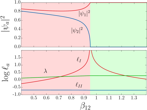
Figure 2.2: The ground state and length-scales of the two-component model (2.12) as functions of the bi-quadratic density coupling $\beta_{12}$, for the parameters $(a_{11},\beta_{11})=(-1,1)$, and $(a_{22},\beta_{22})=(-0.95,1)$. The top panel shows the ground state densities $|\psi_{a}|^{2}$, while the bottom panel shows the relevant length-scales. Depending on the value of $\beta_{12}$, the ground state is either in a miscible phase (red background) or in an immiscible phase (green background). There is clearly a length-scale hierarchy $\ell_{I}>\ell_{II}$, and the penetration depth $\lambda$ can be either the largest length-scale, or intermediate in the vicinity of the symmetry changing transition. Here $e=1$, but since gauge coupling scales the value of $\lambda$, it is clear that there always exist regimes that satisfy the length-scale hierarchy $\ell_{I}>\lambda>\ell_{II}$.

The density and relative phase sectors of the perturbation operator decouple. Moreover, in agreement with the $\mathrm{U}(1)\!\times\!\mathrm{U}(1)$ symmetry of the theory, the perturbations of the relative phase (2.11), the Leggett mode, are massless ${\cal M}_{\phi\phi}^{2}=0$. The remaining non-trivial perturbations are defined by the mass matrix

$${\cal M}_{ff}^{2}=2\left(\begin{array}[]{c c}\alpha_{11}+3\beta_{11}u_{1}^{2}+\beta_{12}u_{2}^{2}&2\beta_{12}u_{1}u_{2}\\ 2\beta_{12}u_{1}u_{2}&\alpha_{22}+3\beta_{22}u_{2}^{2}+\beta_{12}u_{1}^{2}\end{array}\right)\,,$$ (2.15)

whose eigenvalues are $m^{2}_{I}$ and $m^{2}_{II}$ are non-degenerate. As a result, as illustrated on the bottom panel of Fig. 2.2, the corresponding length-scales $\ell_{I}$ and $\ell_{II}$ are also non-degenerate. At the transition between the miscible, and the immiscible phase, the smallest mass $m^{2}_{I}$ becomes massless, and thus $\ell_{I}$ diverges here. On the other hand, the penetration depth $\lambda=1/e\sqrt{u_{1}^{2}+u_{2}^{2}}$ is always finite, even at the transition between the two phases. This implies in particular that the length-scale hierarchy (2.8) can always be realized in a close enough vicinity of the transition.

It is important to emphasize again that $\ell_{I,II}$ corresponds to hybridized modes and cannot be attributed to a given condensate separately. That is, $m^{2}_{I,II}$ are the decay rates of a linear combination of $\psi_{1}$ and $\psi_{2}$.

2.1.3 Long-range intervortex forces

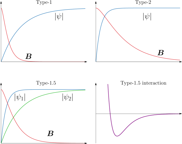
Figure 2.3: The panels on the top row illustrate the vortex profiles in single-component type-1 and type-2 regimes. The bottom left panel shows a vortex profile when the penetration depth is an intermediate length-scale. This allows, in principle, for non-monotonic intervortex forces as illustrated in the bottom right panel.

The analysis of the perturbation operator (2.4), (2.5) not only determines the mass spectrum, the length-scales, and the hybridization of the various modes, but it also determines the asymptotic intervortex forces. The typical vortex profiles are illustrated in Fig. 2.3. The asymptotic behaviour of vortices is determined by the same linearized theory. Assuming that the singularities in the different components overlap, as sketched in Fig. 2.4, the linearized theory yields the following long-range intervortex interaction [156, 155, 164, 158]:

$$E_{\mathrm{int}}(r)=C_{\lambda}K_{0}(r/\lambda)-\sum_{a=I,II,\cdots}C_{a}K_{0}(r/\ell_{a})\,,$$ (2.16)

where $K_{0}$ is the modified Bessel function of the second kind, and $r$ is the distance that separates two vortices. The coefficients $C_{\lambda}$ and $C_{a}$ depend on the eigenstates of the perturbation operator (the normal modes) and on the nonlinearities . The first term describes the repulsion driven by the magnetic and current-current interactions. The second term, associated with the scalar fields, is attractive. Thus, at very large distance $r$, the intervortex interaction $E_{\mathrm{int}}(r)$ is dominated by whichever term corresponds to the largest length-scale. Or equivalently, by the smallest of the masses. The length-scales $\lambda$ and $\ell_{a}$ thus determine whether the vortices attract or repel at long range. The overall asymptotic intervortex interaction (2.16), when the length-scale hierarchy allows for non-monotonic forces, is represented in the bottom right panel of Fig. 2.3.

Figure 2.4: A composite vortex with two co-centred fractional vortices, in the case of a two-component system. Here the singularities of both condensates overlap.

When the penetration depth $\lambda$ is an intermediate length-scale, i.e. for a hierarchy of the length-scale (2.8), the vortices feature a long-range tail of the scalar fields. This results in long-range attractive intervortex forces (dominated by the core-core interactions). On the other hand, at the intermediate scales specified by the penetration depth of the magnetic field, the interactions are dominated by the current-current interactions which are repulsive. It follows that the long-range intervortex interacting potential (2.16) predicted by the linear theory can be long-range attractive and short-range repulsive. This results in non-monotonic intervortex forces, see the calculations in different models [155, 164, 158, 165, 170, 171, 172, 173]. These forces can promote the formation of a bound state of vortices. In such a bound state, the distance separating the vortices does not directly follow from the linearized theory, but it is determined by full nonlinear theory.

Importantly, in multicomponent superconductors, there can be second order phase transitions within the superconducting state. That is, phase transitions for which the total density, and thus the penetration depth $\lambda$ are finite. This is for example the case of the transition between miscible and immiscible phases displayed in Fig. 2.2, see e.g. [174]. Transitions to the time-reversal symmetry breaking $s+is$ state, discussed in more details in the Chapter 3 also occur within the superconducting state, see e.g. [175, 160, 159]. Since second order phase transitions are associated with a divergent length-scale, and that $\lambda$ remains finite, the penetration depth is always an intermediate length-scale close enough to the transition. This implies that in the vicinity such transition the length-scale hierarchy (2.8) is always satisfied.

The analysis of the long-range intervortex forces thus opens the possibility for non-monotonic interaction between composite vortices, that are long-range attractive and short-range repulsive (see e.g. [155, 164, 158]). Thus, the long-range properties can be easily determined by the analysis of the length-scales of the model. However, the length-scale analysis provides only a necessary, yet not sufficient condition for the existence of non-monotonic forces beyond the linear approximation [164, 158]. It is thus necessary to investigate the intervortex forces at the nonlinear level. This was investigated in details at the level of the Ginzburg-Landau theory, and it was demonstrated that non-monotonic forces exist for various kind of potential and also survives the existence of mixed-gradient term [164, 158]. It was further demonstrated that this behaviour can also appear in fully microscopic models [165].

In practice, the demonstration that non-monotonic forces exist at the nonlinear level can be done in the following way. In a descretized system, start with an ansatz that describes to separated vortices (see e.g. Appendix B.2.3, for discussion of such an ansatz). Then relax all degrees of freedom except those corresponding to the core location. After convergence, the resulting configuration is that of two vortices at a certain distance. The energy of such a configuration is thus the energy of two isolated plus the interaction energy between the vortices. Repeating the procedure for various vortex separations provides the interaction energy between the vortices. This procedure was used to determine that two-component superconductors indeed can support non-monotonic forces at the non-linear level [164, 158, 176]. The same procedure was also used to investigate the interactions between three and four vortices [177, 178], and that the nonlinear superposition can result in unusual additional effects. Note also that the criteria that determine the conditions for non-monotonic intervortex interaction can also be supplemented with the analysis of the surface energy between superconducting and normal states [179].

Large systems where vortices are approximated as point particles with the effective non-monotonic interaction revealed an extremely rich physics of vortex structure. Indeed, the multi-scale nature of the interaction allows for vortex arrangements that are much more complicated than the Abrikosov lattices that occur in purely repulsive systems. These include vortex clusters and stripe phases [180, 181, 182], stripe and gossamer phases [183], honeycomb and square lattices [184], multi-stripe phases, polymer phases, void phases [185]. This richness of the large scale organizations have been confirmed in simulations of type-1/type-2 bilayers [186].

2.2 Vortex clusters

The discrepancy of the length-scales thus opens the possibility for long-range attractive and short-range repulsive intervortex forces. It was thus demonstrated that the non-monotonic forces do survive at the nonlinear level [164, 158]. The non-monotonic forces indicate a preferred separation between two vortices. Hence they should form a bound state. When there are more than two-flux quanta, this means that they should form aggregates, or clusters of various shape. This expectation is supported by the analysis of point particle vortices with multi-scale interaction [180, 181, 182, 183, 184, 185].

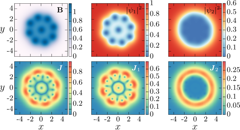
Figure 2.5: A vortex cluster solution of a two-component superconductor, carrying 9 flux quanta. The parameters of the simple potential interaction (2.1c) are $(\alpha_{11},\beta_{11})=(-1,1)$, $(\alpha_{22},\beta_{22})=(-0.6,1)$, and the gauge coupling is $e=1.5$. Here $\alpha_{12}=\beta_{12}=\gamma_{12}=0$, thus the theory as a $\mathrm{U}(1)\!\times\!\mathrm{U}(1)$ symmetry. The displayed quantities on the top left panel is the magnetic field. The other panels on the top row, show the individual densities of the superconducting condensates $|\psi_{1}|^{2}$ and $|\psi_{2}|^{2}$. The bottom left panel shows the total current, while the other panels on the bottom row, are the individual currents ${\bm{J}}_{a}$. The color map here shows the magnitude of the supercurrents $|{\bm{J}}_{a}|$. This is a close view of the cluster, but the actual numerical grid is larger.

These strong indications of the existence of clusters should however be investigated in details, at the nonlinear level of the original Ginzburg-Landau theory. The numerical minimization of multi-vortex states, in the regime of non-monotonic interactions, shows that two-component Ginzburg-Landau models indeed allow the formation vortex clusters [JG27.], as illustrated for example in Fig. 2.5 . The discretization method, the choice of the numerical algorithm, and the general procedure are presented in details in the Appendix B. Yet this can be outlined as follows: The (nonlinear) minimization algorithm typically converges easily to the solution, provided a suitable initial guess. In short, an initial field configuration which winds $n$ times in each of the condensate will converge to a configuration that carries $n$ flux quanta (see detailed discussion in Section B.2.3). Provided the parameter set allows for non-monotonic forces this typically results in a cluster carrying $n$ flux quanta, as that displayed in Fig. 2.5.

As can be seen from the density panels of Fig. 2.5, the first component clearly forms nine vortices that repel each other like in type-2 superconductors. The second component, on the other hand, is almost fully depleted inside the vortex cluster (like in the type-1). Finally, there is a clear overlap of the magnetic field of the different vortices. Here, the interesting feature is that the cluster clearly comprises between the tendencies of the different condensates. Indeed, the first component tends to form a regular vortex lattice, while the second condensate favours a circular normal domain with a supercurrent predominantly located on the boundary. This competition between forming a circular cluster, and a triangular lattice leads to a variety of clusters which are neither an hexagonal lattices nor a fully circular boundary. For more details of the various possible cluster, see [JG27.].

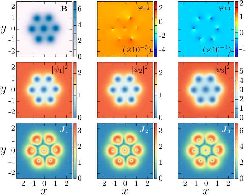
Figure 2.6: A vortex cluster solution of three-component superconductor, with the parameters of the potential term (2.1c) are $(\alpha_{11},\beta_{11})=(\alpha_{22},\beta_{22})=(-3,3)$, $(\alpha_{33},\beta_{33})=(2,0.5)$, $\alpha_{12}=2.25$ $\alpha_{13}=\alpha_{23}=-3.7$ and the gauge coupling is $e=1.35$. The other parameters are $\beta_{ab}=\gamma_{ab}=0$. The displayed quantities on the top row are the magnetic field and two relative phases $\varphi_{12}$ and $\varphi_{13}$. The middle row shows the densities of the three components $|\psi_{a}|^{2}$, from which it is clear that the cores in the different components have different sizes. The panels on the bottom row displays the associated super-currents ${\bm{J}}_{a}$. Interestingly, as can be seen from the relative phase panels, the cores in the different components do not fully overlap at the exterior of the cluster.

The existence of vortex aggregates due to non-monotonic intervortex forces easily promotes to more than two components. The figure 2.6 shows an example of a vortex cluster in the case of a three-components model. The case of vortex clusters occurring in three-components models was demonstrated in details in [JG25.]. Unlike the cluster illustrated in Fig. 2.5 all components of the cluster in Fig. 2.6 form vortices with different core sizes. While the cluster in Fig. 2.5 had to comprise between type-1-like and type-2-like behaviours, the cluster in Fig. 2.6 easily fits with a triangular lattice.

Remark about the hybridization:

In single-component Ginzburg-Landau model, the coherence length can easily be guessed from the size of the vortex cores. This is not true in general for in multicomponent models. Indeed, as already discussed in the previous section, the length-scale analysis shows that the various modes are in general hybridized, and thus that it is not possible to attribute a single length-scale to a given condensate. This is especially the case when there are phase-locking terms. Thus inspection of the vortex core sizes can easily the discrepancy of the length-scales. The cluster illustrated in Fig. 2.6 is a good example of this: The cores in the different condensates seems to have almost the same sizes. Yet there is a strong cluster structure.

2.3 Formation of vortex clusters. Realization of semi-Meissner states

The vortex clusters presented above are found numerically by the minimization of the Ginzburg-Landau free energy, given an initial guess with the appropriate winding, see details in the Appendix B. They thus represent vortex clusters surrounded by voids of the Meissner state. Hence the terminology semi-Meissner state. The properties of the semi-Meissner state can also be investigated in an external applied field ${\bm{H}}_{e}$, by minimizing the Gibbs free energy,

$$G=F-\int{\bm{B}}\cdot{\bm{H}}_{e}\,,$$ (2.17)

instead of the Helmholtz free energy $F$ (2.1). Thus simulations in increasing values of the external field ${\bm{H}}_{e}$, reproduce the magnetization curves sketched in Fig. 2.1. Complementary to the investigation of the magnetization properties, are simulations that mimic field cooled experiments. Indeed for realistic models, the various parameters are temperature dependent. For example, the parameters of the quadratic terms depend on the temperature $T$ as $\alpha_{aa}\equiv\alpha_{aa}(T)=\alpha_{aa}^{(0)}(T/T_{c,a}-1)$. Here $\alpha_{aa}^{(0)}$ is the value of the coefficient at zero temperature, while $T_{c,a}$ is the characteristic temperature where the condensate $\psi_{a}$ becomes active. Here “active", means: The temperature below which $\psi_{a}$ would condense, if decoupled from the other condensates.

A magnetization process thus accounts to a vertical line in the $H-T$ phase diagrams sketched in Fig. 2.1. A field cooled experiment on the other hand accounts to an horizontal line in the $H-T$ phase diagrams. In practice, in numerical simulations, a magnetization process is realized by minimizing the Gibbs energy (2.17), at a given value of the applied field ${\bm{H}}_{e}$. After convergence, then the value of ${\bm{H}}_{e}$ is increased/decreased, and the procedure is repeated for the new value of the external field. Likewise, a field cooled experiment is simulated by by minimizing the Gibbs energy in an external field ${\bm{H}}_{e}$, at a given value of the parameters $\alpha_{aa}(T)$. Then, after convergence, the temperature modified, and the minimization is restarted for the new parameters $\alpha_{aa}(T+\delta T)$. Surely, simulating such processes is much more time consuming than the construction of (isolated) topological defects.

It should be expected that the magnetic response near the second critical field $H_{c2}$, or in the vicinity of the critical temperature, reduces to single-component. See for example the discussions [165, 187, 188] or the reviews [177, 189, 190]. This can also be seen from the high field behaviour of the magnetization curve in Fig. 2.1. Indeed, in high field, there is no way to tell the difference between the magnetization curve of type-1.5 and usual type-2. Heuristically this follows from the fact that the intervortex distance in a vortex lattice become small. In that case, the vortex attractionis too weak, and the vortices are not “free” to form aggregates.

However, at lower temperature the non-monotonic forces can set in and lead to the formation of vortex clusters. This is again sketched in Fig. 2.1. Thus, in a field cooled experiment the Abrikosov lattice can collapse into clusters at low temperatures. This was confirmed for example in simulations for clean interface superconductors [JG17.]. Measurement of the flux carrying area thus show that clusters form. Indeed, the flux carrying area, illustrated in Fig. 2.7, is defined as

$$\text{Flux carrying area}=\int\Theta\left({\bm{B}}/B_{\mathrm{max}}-\delta_{\bm{B}}\right)\,.$$ (2.18)

Here $\Theta$ is the Heaviside step function, $\delta_{\bm{B}}$ some tolerance, and $B_{\mathrm{max}}$ is the maximal value of the magnetic field. The local internal flux density of the flux carrying regions is the value of the magnetic field, averaged over the flux carrying regions. This can be formally defined as:

$$\text{Internal flux density}=\frac{\int\Theta\big{(}|{\bm{B}}|/B_{max}-\delta_{\bm{B}}\big{)}|{\bm{B}}|}{\int\Theta\big{(}|{\bm{B}}|/B_{max}-\delta_{\bm{B}}\big{)}}\,.$$ (2.19)

The internal flux density should show a strong peak where the attractive intervortex forces are strongest and where thus the clusters are the most compact. These effects for the clusterization was discussed in [JG5.], in the context of dirty two-band superconductors.

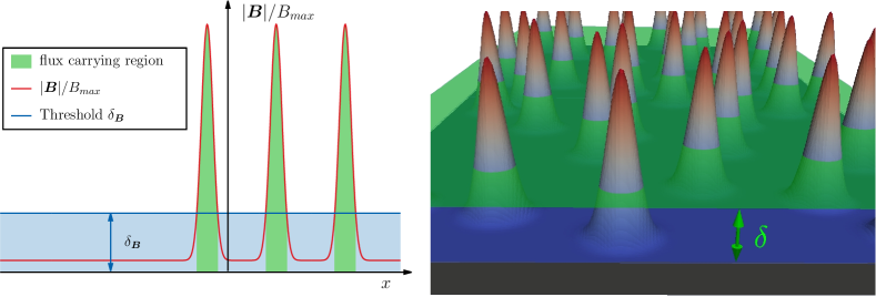
Figure 2.7: Principle to determine the fraction of sample containing flux. For a given distribution of the magnetic field, the regions for which the magnetic field is below a threshold value $\delta_{\bm{B}}B_{max}$ are said to be in the Meissner state. Conversely, regions for which $|{\bm{B}}|>\delta_{\bm{B}}B_{max}$ are the flux carrying regions.

Models with semi-Meissner states

In all the discussions above, all parameters of the Ginzburg-Landau theory are given as free parameters. This is of course not the case in real life, where the various parameters cannot in general be chosen independently. Thus, taking into account the underlying microscopic properties of a given model of superconductivity constraints the relation between the various parameters. In particular, the various parameters are temperature dependent. It follows that the conditions for the realization of the type-1.5 regime, may be satisfied only in a given interval of the temperature. Moreover, it is quite expectable that if vortex bound states are formed, their typical size should also be temperature dependent.

Various works investigated the possibility to realize semi-Meissner states from realistic microscopic theory of multi-band superconductors, see e.g. [165, 191, 80]. Also models for clean interface superconductors, such as SrTiO₃/LaAlO₃ predict the unconventional magnetic response due to non-monotonic intervortex forces [JG17.].

Also dirty two-band superconductors can feature a second order phase transition to the ${s\!+\!is}$ state that breaks the time-reversal symmetry see e.g. [JG9.] and [JG5.]. In the vicinity of such a transition, the necessary length-scale hierarchy should be realized, thus opening the possibility for cluster formation. This was discussed in more details [JG25.] and [JG5.]. See also the related discussion in the next chapter.

Applicability and experimental relevance

In the regime where the penetration depth is an intermediate length-scale, vortices can thus have a long-range attractive and short-range repulsive interaction. It follows that vortices can aggregate into clusters surrounded by Meissner domains. Experimental works using magnetic decoration, scanning SQUID and scanning Hall probes measurements reported inhomogeneous vortex distribution on clean superconducting material MgB₂ [154, 192, 181]. Being a two-band material, the very inhomogeneous distribution of vortices was attributed to non-monotonic forces originating from the competing type-1 and type-2 behaviours. This regime was termed “type-1.5 superconductivity" [154]. When cycling field, the observation that the vortex clusters form in different parts of the sample, allows to rule out the alternative explanation that the observed aggregation is due to pinning.

Several experimental works reported local vortex coalescence in layered-perovskite superconductor Sr₂RuO₄ [193, 194, 195, 196]. The semi-Meissner state was proposed to be responsible for the aggregates observed in Sr₂RuO₄. This proposal followed from both theoretical [JG22.], and experimental scanning SQUID [197], and muon-spin rotation measurements [157]. There, it was observed that the vortex clusters contract upon temperature decrease, well below $T_{c}$. This behaviour hints for attractive inter-vortex forces, rather than pinning, to be responsible for the cluster formation. Note that earlier experiment also reported attractive inter-vortex forces, which were attributed to domain walls trapping vortices [193]. However signatures domain-walls were not observed in surface probes [197].

The scenario of vortex coalescence attributed to the semi-Meissner regime received experimental support as well in other superconducting material such as LaPt₃Si [198, 199]. Further theoretical predictions argued that the type-1.5 regime could be realized as well for certain interface superconductors SrTiO₃/LaAlO₃ [JG17.], and should generically be present near transitions from $s$ to ${s\!+\!is}$ pairing states in iron-based superconductors [JG25.] and [JG25.]; or in the context of dirty two-band materials [JG5.].

For other works on this and related subjects see e.g. [200, 181, 201, 202, 203, 182, 178, 184, 174, 204, 185].

Controversy about the existence of type-1.5 regime.

Note that the possibility to realize type-1.5 regime was heavily debated on theoretical grounds [205, 206, 188, 207]. In my view the question is sorted and there is no doubt that this phenomenon do exist. This follows the accumulation of theoretical and numerical works demonstrating the existence of this regime. Moreover one of the earlier works claiming of inexistence of the type-1.5 regime [206, 206] bases its conclusions on an erroneous set of equations; for the detailed demonstration, see [190]. Using the equations obtained by this incorrect derivation, several further papers propagated misconceptions about the possibility of having a type-1.5 regime. Having in mind that the objections, against the existence of type-1.5 regime, originate into incorrect equations, there is no doubt about the theoretical relevance of such a physics. While there is no reason to doubt about the theoretical possibility of the type-1.5 regime, there is no guarantee that this is realized in nature. Note however, that as mentioned above, several experiments are consistent with that physics.

Chapter 3 Superconducting states that Break the Time-Reversal Symmetry

Theories that describe the physics of superconductors (or superfluids) are invariant under complex conjugation. This invariance is usually referred to as the time-reversal symmetry (TRS). As already emphasized, the properties of multicomponent superconducting states can be qualitatively different from their simplest single-band $s$-wave counterparts. In multicomponent systems, the time-reversal symmetry can be spontaneously broken by the ground state. That is, the ground state is not invariant (up to global phase rotations) under complex conjugation. Such states can appear if the relative phase, between the superconducting gap functions in the different bands, differ from $0$ or $\pi$ [208, 209, 210, 146, 211, 212, 145, 213, 171, 214, 215, 216]. It results that, in addition to the breakdown of the usual $\mathrm{U}(1)$ gauge symmetry, such superconducting states feature a discrete $\mathbb{Z}_{2}$ degeneracy, associated with the spontaneous breakdown of the time-reversal symmetry (BTRS).

Spontaneously broken time-reversal symmetry (BTRS) states attracted much interest in the context of unconventional spin-triplet superconducting models, especially the $p_{x}+ip_{y}$ state, which have been intensively studied in relation with layered perovskite superconductor Sr₂RuO₄ . Another time-reversal symmetry breaking state, which attracted more recently a lot of attention, is the ${s\!+\!is}$ superconducting state. Indeed, it received a strong theoretical support in relation with some iron-based superconductors, and in particular with hole-doped Ba_1-xK_xFe₂As₂ [217, 218, 219, 220, 215]. The ${s\!+\!is}$ state is of particular interest, as it is the simplest time-reversal symmetry breaking extension of the most abundant $s$-wave state. It is a complex admixture of distinct superconducting states, with the same symmetry, that compete through phase-locking terms. In pnictides, it is believed to originate in the competition between different pairing channels [215], but could as well be engineered on interfaces of superconducting bilayers [145].

The spontaneous breakdown of the time-reversal symmetry has various interesting physical consequences. Some of which, like the existence of domain-walls, where earlier discussed in Chapter 1. Iron-based superconductors [60] are among the most promising materials for the observation of the time-reversal symmetry breaking ${s\!+\!is}$ states that originate in the multiband character of superconductivity and several competing pairing channels. Indeed, the experimental data show that in the hole-doped 122 compounds Ba_1-xK_xFe₂As₂, the symmetry of superconducting state can change depending on the doping level $x$. A typical band structure of Ba_1-xK_xFe₂As₂ consists of two hole pockets at the $\Gamma$ point and two electron pockets at $(0,\pi)$ and $(\pi,0)$. At moderate doping level $x\sim 0.4$ various measurements, including ARPES [221, 222, 223], thermal conductivity [224] and neutron scattering experiments [225], are consistent with the hypothesis of an $s_{\pm}$ state where the superconducting gap changes sign between electron and hole pockets. On the other hand, the symmetry of the superconducting state at strong doping $x\rightarrow 1$ is not so clear, regarding the question whether the $d$ channel dominates or if the gap retains $s_{\pm}$-symmetry changing sign between the inner hole bands at the $\Gamma$ point [218, 219]. Indeed, there are evidences that $d$-wave pairing channel dominates [226, 227, 228, 229] while other ARPES data were interpreted in favour of an $s$-wave symmetry [230, 231]. In both situations this implies the possible existence of an intermediate complex state that compromises between the behaviours at moderate and high doping. Depending on whether $d$ or $s$ channel dominates at strong doping such a complex state is named ${s\!+\!is}$ or ${s\!+\!id}$. Both of these superconducting states break the time-reversal symmetry.

The ${s\!+\!is}$ state is isotropic and preserves crystal symmetries [215]. On the other hand, the ${s\!+\!id}$ state breaks the $C_{4}$ symmetry, while it remains invariant under combination of time-reversal symmetry operation and $C_{4}$ rotations. Being anisotropic, it is thus qualitatively different from ${s\!+\!is}$ state. Note that the ${s\!+\!id}$ superconducting state is also qualitatively different from the (time-reversal preserving) $s+d$ states that attracted interest in the context of high-temperature cuprate superconductors (see e.g. [232, 233, 234]). It also contrasts with $d+id$ state, which can appear in the presence of an external magnetic field, and that violates both parity and time-reversal symmetries [208, 235] . While it is an interesting scenario, possibly relevant for pnictides, the properties of the ${s\!+\!id}$ state will not be further considered here. The focus will be put on the analysis of ${s\!+\!is}$ superconducting state. This state is of particular theoretical interest, being the simplest extension of the most abundant $s$-wave state, that breaks the time-reversal symmetry. Also, it is expected to arise from various microscopic physics [146, 210, 236, 63, 215, 237]. The ${s\!+\!is}$ state could as well be fabricated on demand on the interfaces of superconducting bilayers [145].

The experimental observation of the ${s\!+\!is}$ or ${s\!+\!id}$ time-reversal symmetry breaking states is challenging. Indeed, this requires probing the relative phases between the components of the order parameter in different bands, which is a challenging task. For example the ${s\!+\!is}$ state does not break the point group symmetries and is therefore not associated with an intrinsic angular momentum of the Cooper pairs. Consequently it cannot produce a local magnetic field and thus is a priori invisible for conventional methods like muon spin relaxation and polar Kerr effect measurements that were for example used to probe time-reversal breaking ${p\!+\!ip}$ superconducting state in e.g. Sr₂RuO₄ compound [58]. Several proposals were voiced, each with various limitations, for indirect observation of BTRS signatures in pnictides. These, for example, include the investigation of the spectrum of the collective modes which includes massless [213] and mixed phase-density [171, 238, 215, 239] excitations. Also, it was proposed to consider the properties of exotic topological excitations such as skyrmions and domain walls [142, 120, 119], unconventional mechanism of vortex viscosity [240], formation of vortex clusters [171], exotic reentrant and precursor phases induced by fluctuations [241, 242, 243, 244]. Moreover, spontaneous currents were predicted to exist near non-magnetic impurities in anisotropic superconducting ${s\!+\!id}$ states [209, 216] or in samples subjected to strain [216]. The latter proposal actually involves symmetry change of ${s\!+\!is}$ states and relies on the presence of disorder, which can typically have uncontrollable distribution. It was also pointed out that the time-reversal symmetry breaking ${s\!+\!is}$ state features an unconventional contribution to the thermoelectric effect [245]. Related to this an experimental set-up, based on a local heating was recently proposed [246]. The key idea being that local heating induces local variations of the relative phases, which further yield an electromagnetic response that is directly observable.

Plan of the Chapter

The existence of the ${s\!+\!is}$ state can originate from various mechanisms, including the competition between different pairing channels, or impurity scattering. These aspects will not be addressed here. Instead we will discuss how this ${s\!+\!is}$ state appears in phenomenological Ginzburg-Landau models. Discussions of the microscopic origin of the ${s\!+\!is}$ state, and its relation to Ginzburg-Landau models was for example discussed in [JG14.] and [JG10.]. See also [JG9.] and [JG5.] for discussions of the ${s\!+\!is}$ state that originates in impurity scattering.

As a starting point, the Section 3.1 presents the mechanism of phase frustration, that is responsible for the spontaneous breakdown of the time-reversal symmetry, in three-component superconductors. Namely, this is the competition between different phase-locking terms that can result in the ${s\!+\!is}$ state. Since the time-reversal symmetry is a discrete operation, its spontaneous breakdown implies that the ground state features a discrete degeneracy. The properties of such ground state will be analyzed in Section 3.1.1, while the corresponding length-scales are derived in Section 3.1.2. The case of a two-component ${s\!+\!is}$ state will also be addressed in this section.

Next, the properties of topological defects that can occur in superconducting states which break the time-reversal symmetry are addressed in the Section 3.2. There is some overlap with the discussions of Section 1.3.3 of the Chapter 1. The fact that the ground state breaks a discrete symmetry implies that the theory allow for domain-wall excitations. These domain-walls between different time-reversal symmetry broken states are constructed in Section 3.2.1. The domain-walls interact non-trivially with the vortex matter. As detailled in Section 3.2.2, closed domain-walls can form bound states with vortices. As discussed in the Chapter 1, since the resulting composite defects are coreless, they feature extra topological properties: they are the chiral $\mathbb{C}\mathrm{P}^{2}$ skyrmions.

Finally, in the thermoelectric properties of the ${s\!+\!is}$ state will be discussed in Section 3.3. The new thermoelectric properties of the ${s\!+\!is}$ state are consequences of the modified current, and magnetic relations in multicomponent superconductors.

Summary of the results that are relevant for this chapter

• In [JG10.] we have demonstrated that the mean field theories for the $s\!+\!is$ superconducting states, that break the time-reversal symmetry, are quantitatively consistent with microscopic multi-band models. We have further demonstrated that the $s\!+\!is$ state can also appear in two-band systems due to impurity scattering [JG9.]. Within the quasiclassical approximation we show that the $s\!+\!is$ state forms as an intermediate phase at the impurity-driven crossover between $s_{\pm}$ and $s_{++}$ states. We further established in [JG10.] and [JG5.] that the $s\!+\!is$ domain is surrounded by a line of second-order phase transition, which implies the existence of a soft mode with a divergent length-scale. The other coherence lengths remain finite at this transition and thus there is an infinite disparity of coherence lengths, which may lead to unusual vortex physics with non-monotonic forces [JG5.] and [JG6.].

• In [JG14.] and [JG12.] we have demonstrated that the existence of time-reversal symmetry broken states measurably impacts the thermoelectric response of superconductors. In [JG14.] we predicted that superconductors which break the time-reversal symmetry feature a giant thermoelectric effect of principally different nature than that in single-component superconductors. It originates in thermally induced intercomponent counterflows, in contrast to the counterflows of normal and superconducting currents in the classical Ginzburg mechanism. We have further demonstrated in [JG12.] that these unconventional thermoelectric properties can be used to induce experimentally observable magnetic and electric fields by local heating of candidate materials. The induced fields are sensitive to the presence of domain-walls and crystalline anisotropy, while nonstationary heating process produces an electric field and a charge imbalance in the different bands [JG12.].

• Prediction of the experimental signatures of domain-wall structures that form during quenches, via the Kibble-Zurek mechanism, in superconductors with broken time-reversal symmetry originating in ${s\!+\!is}$ gap structure [JG19.]. As it is a discrete symmetry, the spontaneous breakdown of the time-reversal symmetry in the ${s\!+\!is}$ state, dictates that it possess domain wall excitations. We also discuss the influence of geometrically stabilized domain-walls on the magnetization processes.

• Discovery of a new kind of stable topological solitons in three-component superconductors that spontaneously breaks the time-reversal symmetry [JG26.] and [JG21.]. These flux carrying topological defects, are characterized by a hidden topological charge, associated with the topology of the complex projective space $\mathbb{C}\mathrm{P}^{N-1}$. These $\mathbb{C}\mathrm{P}^{2}$ skyrmions can spontaneously form in field cooled experiment [JG19.], when the cooling process goes through the phase transition to the time-reversal symmetry broken state.

• Findings of a new kind of collective mode in three-band superconductors with broken time-reversal symmetry [JG25.]. This collective mode is associated with mixed phase-density collective excitations. Thus it is different from the Leggett’s mode.

3.1 Phase frustration in three-band superconductors

The time-reversal symmetry breaking ${s\!+\!is}$ states occurs due to the competition between different pairing channels. At the level of the mean field theory, this manifests itself through the existence of competing phase-locking terms. When different phase-locking terms cannot be simultaneously satisfied, the system may comprise via non-trivial relative phases between the condensates [145, 146, 247, 248]. It was indeed observed that the inclusion of a third superconducting condensate leads to qualitatively different physics compared to two-component systems [145, 146, 247, 248]. As detailed below, the states with non-trivial relative phases (i.e. when at least one is neither $0$ nor $\pi$) break the time-reversal symmetry.

To illustrate how phase frustration leads to the spontaneous breakdown of the time-reversal symmetry, we consider here a restriction of the generic free energy (1), for three superconducting condensates coupled via bilinear Josephson interaction:

$$\mathcal{F}/\mathcal{F}_{0} =\bigintsss\frac{1}{2}\big{|}{\bm{\nabla}}\!\times\!{\bm{A}}\big{|}^{2}+\sum_{a=1}^{3}\frac{1}{2}\big{|}{\bm{D}}\psi_{a}\big{|}^{2}+V(\Psi,\Psi^{\dagger})\,,$$ (3.1a)

$$\text{where}\leavevmode\nobreak\ V(\Psi,\Psi^{\dagger}) =\sum_{a=1}^{3}\left(\alpha_{a}|\psi_{a}|^{2}+\frac{1}{2}\beta_{a}|\psi_{a}|^{4}\right)+\sum_{a=1}^{3}\,\sum_{b>a}^{3}\eta_{ab}(\psi_{a}^{*}\psi_{b}+\psi_{b}^{*}\psi_{a})\,,$$ (3.1b)

Here again, $\psi_{a}=|\psi_{a}|e^{i\varphi_{a}}$ are complex fields representing the three superconducting condensates labelled by the indices $a,b=1,2,3$. For simplicity, mixed gradient terms are not considered (namely $\kappa_{ab}=\delta_{ab}$). Besides the electromagnetic coupling, the different condensates are directly coupled via the (bilinear) Josephson interaction:

$$\eta_{ab}(\psi_{a}^{*}\psi_{b}+\psi_{b}^{*}\psi_{a})=2\eta_{ab}|\psi_{a}||\psi_{a}|\cos(\varphi_{ab})\,,$$ (3.2)

where $\varphi_{ab}=\varphi_{b}-\varphi_{a}$ denotes the relative phase between two condensates. Such a multicomponent Ginzburg-Landau free energy can, in certain cases, be derived microscopically at temperatures close to $T_{c}$ (for a review see [249], see also [JG10.]). Note that the existence of three superconducting bands is not by any means a sufficient condition for a system to have Ginzburg-Landau expansion like that displayed in (3.1). However many of the question of phase-frustration which is considered here, do not require to be in the high-temperature region where the Ginzburg-Landau expansion (3.1) can be formally justified. In the following, the minimal Ginzburg-Landau model (3.1) is used as a convenient framework to discuss qualitatively the physics of phase frustration, and how it leads to time-reversal symmetry breaking. Discussions on microscopic physics aspects can be found, for example, in [JG6.], [JG10.], and [JG9.]. Note that three-component models feature in principle additional terms allowed by symmetry, e.g. bi-quadratic terms in density (see for example [120]). However these terms play a little role in the phase frustration that leads to the breakdown of the time-reversal symmetry. Hence we focus here on the simplest model.

The quartic coefficients $\beta_{a}$ are positive so that the free energy (3.1) is bounded from below. On the other hand, the quadratic coefficients $\alpha_{a}$ change signs at some characteristic temperatures which are generally different for all components. Below this characteristic temperature $\alpha_{a}<0$ and the band is said to be active, while above it, $\alpha_{a}>0$ and the band is passive. Nevertheless, passive bands can feature nonzero superfluid density because of the interband Josephson tunnelling terms with the coupling $\eta_{ab}$. For the superconducting state to exist, the determinant of the second order couplings should be negative . Hence, for the potential (3.1b), the superconducting states exists if

$$\alpha_{1}\alpha_{2}\alpha_{3}+2\eta_{12}\eta_{13}\eta_{23}-\alpha_{1}\eta_{23}^{2}-\alpha_{2}\eta_{13}^{2}-\alpha_{3}\eta_{12}^{2}<0\,.$$ (3.3)

Figure 3.1: Schematic illustration of phase locking patterns. Panels (a) and (b) show the two possible phase locking for two components; either zero or $\pi$. Panels (c), (d) and (e) display the possible, qualitatively different, phase locking in the case of three components. Panels (c) and (e), the relative phases are said to be trivial (i.e. either zero or $\pi$). The case of the panel (d) is a three frustrated component superconductor, with non-trivial phase locking.

When the parameters satisfy the condition (3.3), systems with more than two condensates can exhibit frustration of the competing Josephson coupling terms. When $\eta_{ab}<0$, a given Josephson interaction term (3.2) is minimal for zero relative phase $\varphi_{ab}$, and this coupling is a “phase-locking". On the other hand, when $\eta_{ab}>0$, the Josephson interaction is minimal for the relative phase $\varphi_{ab}=\pi$, and this coupling is a “phase-antilocking" . The behaviour of the individual phase-locking terms between two condensates is illustrated in Fig. 3.1. There, the panel (a) shows a relative phase $\varphi_{12}=\pi$, and thus corresponds to $\eta_{12}>0$. Panel (b) on the other hand shows the zero relative phase that minimizes the Josephson interaction for a negative Josephson coupling $\eta_{12}<0$.

Now, in the case of three condensates, depending on the signs of the couplings $\eta_{ab}$, the individual Josephson terms cannot always be simultaneously minimal. Indeed, the relative phases are not all independent; for example

$$\varphi_{23}:=\varphi_{3}-\varphi_{2}=\varphi_{3}-\varphi_{1}+\varphi_{1}-\varphi_{2}:=\varphi_{13}-\varphi_{12}.$$ (3.4)

Such a situation, where the phase-locking terms compete with each other, and where the system comprises between the individual tendencies, is called frustrated. Note that, as detailed below, frustration in three-component systems like (3.1) is a necessary (yet not sufficient) condition for the spontaneous breakdown of the time-reversal symmetry. The condition for frustration can be determined in terms of the sign of the Josephson couplings $\eta_{ab}$. Indeed there are four principal situations, summarized in the Table. 3.1. Note that frustration also occurs in the general case of arbitrary number of components. There are more possibilities for such systems to be frustrated, which allows for even richer physics than in three-components. Frustration in four-component systems was discussed in details in [250].

Case	Sign of $\eta_{12},\eta_{13},\eta_{23}$	Ground state phases
1	$---$	$\varphi_{1}=\varphi_{2}=\varphi_{3}$
2	$--+$	Frustrated
3	$-++$	$\varphi_{1}=\varphi_{2}=\varphi_{3}+\pi$
4	$+++$	Frustrated

Table 3.1: Illustration of the qualitatively different representative situation in the case of three-component superconducting condensates coupled via bilinear Josephson interaction. Depending of the sign of the $\eta_{ab}$, there are four principal situations. The ground state phases are given when the signatures do not lead to frustration.

Example of phase frustration and broken time-reversal symmetry:

The simplest illustration of phase frustration is the case where the coefficients of the three components are completely symmetric, and all Josephson couplings are repulsive. For example, with the individual couplings $\alpha_{a}=-1$, $\beta_{a}=1$ for $a=1,2,3$, and the Josephson couplings $\eta_{12}=\eta_{13}=\eta_{23}=-1$. Each individual phase-locking term favours relative phases that equal $\pi$. This is however impossible, since, e.g.

$$\text{if}\leavevmode\nobreak\ \leavevmode\nobreak\ \leavevmode\nobreak\ \varphi_{12}=\varphi_{13}=\pi\,,\leavevmode\nobreak\ \leavevmode\nobreak\ \text{then}\leavevmode\nobreak\ \leavevmode\nobreak\ \leavevmode\nobreak\ \varphi_{23}\equiv\varphi_{13}-\varphi_{12}=0\neq\pi\leavevmode\nobreak\ \leavevmode\nobreak\ \leavevmode\nobreak\ \leavevmode\nobreak\ \leavevmode\nobreak\ (\text{with}\leavevmode\nobreak\ \leavevmode\nobreak\ \varphi_{ab}=\varphi_{b}-\varphi_{a})\,.$$

Hence, since the individual phase-locking terms cannot be simultaneously satisfied, the system is said to be frustrated. Instead, the ground state has all the relative phases equal to $\pm 2\pi/3\mod 2\pi$. More precisely, it can be shown that

$$\text{either}\leavevmode\nobreak\ \leavevmode\nobreak\ \leavevmode\nobreak\ \varphi_{12} =+2\pi/3\,, \varphi_{13} =-2\pi/3\,, \varphi_{23} =+2\pi/3\mod 2\pi\,,$$ (3.5a)

$$\text{or}\leavevmode\nobreak\ \leavevmode\nobreak\ \leavevmode\nobreak\ \varphi_{12} =-2\pi/3\,, \varphi_{13} =+2\pi/3\,, \varphi_{23} =-2\pi/3\mod 2\pi\,.$$ (3.5b)

Figure 3.2: Schematic illustration of the two inequivalent ground states (3.5). Since both configurations are mirror of each others, these states are also referred to as chiral states. The circulating arrows denote circulating interband tunneling currents.

Here, not only the system is frustrated, but also it features a discrete degeneracy. Indeed, since the relative phases are gauge invariant, both configurations (3.5a) and (3.5b) cannot be transformed into each other by a global phase rotation. Both these configurations are displayed in Fig. 3.2. They are related to each other by the complex conjugation, associated with the time-reversal transformation $\mathcal{T}(\psi_{a})=\psi_{a}^{*}$. Since $\mathcal{T}(\varphi_{ab})=-\varphi_{ab}$, the two ground states are indeed related to each other by the time-reversal transformation. Hence the ground state is said to spontaneously break the time-reversal symmetry.

The ground state here, thus features a discrete $\mathrm{U}(1)\!\times\!\mathbb{Z}_{2}$ degeneracy. In a phase transition the ground state randomly picks either of the chiralities, and this may lead to the formation of domain-walls via the Kibble-Zurek mechanism [12, 13]. This was further discussed in [JG19.] and in Sec. 1.3.3. See also the continued discussion in Sec. 3.2.1. Under certain conditions, the spontaneous breakdown of the time-reversal symmetry also allows for composite topological excitations which are bound states of closed domain walls and vortices [142, 120], see Sec. 1.3.3 and the continued discussion in Sec. 3.2.2.

3.1.1 Ground state of a three-component superconductor

As discussed above, frustration occurs depending on the signatures of the different Josephson couplings, as summarized in Table 3.1. Frustration is a necessary, yet not sufficient, condition for the spontaneous breakdown of the time-reversal symmetry. The breakdown occurs depending on the relative values of the Josephson couplings. The dependence of the ground state, with respect to a given coupling illustrates this. The ground state values of the fields $|\psi_{a}|$ and $\varphi_{ab}$ of the free energy (3.1) are found by minimizing its potential energy:

$$\Psi_{0}=\underset{\Psi\in\mathbbm{C}^{N}}{\mathrm{argmin}}\leavevmode\nobreak\ V(\Psi,\Psi^{\dagger})\,,\leavevmode\nobreak\ \leavevmode\nobreak\ \text{with}\leavevmode\nobreak\ \leavevmode\nobreak\ V=\sum_{a=1}^{3}\Bigg{\{}\alpha_{a}|\psi_{a}|^{2}+\frac{1}{2}\beta_{a}|\psi_{a}|^{4}+\sum_{b>a}^{3}\eta_{ab}|\psi_{a}||\psi_{b}|\cos\varphi_{ab}\Bigg{\}}\,.$$ (3.6)

The ground state is determined by the system of equations given by the variations of the potential, with respect to the physical degrees of freedom $|\psi_{a}|$ and $\varphi_{a}$. The variation with respect to the densities read explicitly

$$\frac{\delta V}{\delta|\psi_{1}|}:=2\alpha_{1}|\psi_{1}|+2\beta_{1}|\psi_{1}|^{3}+\eta_{12}|\psi_{2}|\cos\varphi_{12}+\eta_{13}|\psi_{3}|\cos\varphi_{13} =0\,,$$ (3.7a)

$$\frac{\delta V}{\delta|\psi_{2}|}:=2\alpha_{2}|\psi_{2}|+2\beta_{2}|\psi_{2}|^{3}+\eta_{12}|\psi_{1}|\cos\varphi_{12}+\eta_{23}|\psi_{3}|\cos\varphi_{23} =0\,,$$ (3.7b)

$$\frac{\delta V}{\delta|\psi_{3}|}:=2\alpha_{3}|\psi_{3}|+2\beta_{3}|\psi_{3}|^{3}+\eta_{13}|\psi_{1}|\cos\varphi_{13}+\eta_{23}|\psi_{2}|\cos\varphi_{23} =0\,.$$ (3.7c)

Variations of with respect to the phases, on the other hand, read as

$$\frac{\delta V}{\delta\varphi_{1}}:=+\eta_{12}|\psi_{1}||\psi_{2}|\sin\varphi_{12}+\eta_{13}|\psi_{1}||\psi_{3}|\sin\varphi_{13} =0\,,$$ (3.8a)

$$\frac{\delta V}{\delta\varphi_{2}}:=-\eta_{12}|\psi_{1}||\psi_{2}|\sin\varphi_{12}+\eta_{23}|\psi_{2}||\psi_{3}|\sin\varphi_{23} =0\,,$$ (3.8b)

$$\frac{\delta V}{\delta\varphi_{3}}:=-\eta_{13}|\psi_{1}||\psi_{3}|\sin\varphi_{13}-\eta_{23}|\psi_{2}||\psi_{3}|\sin\varphi_{23} =0\,.$$ (3.8c)

The potential is invariant under global rotation of all phases. Thus it can be convenient to fix the gauge by imposing the value of one of the phases, for example $\varphi_{1}=0$. In that case, the equation $\delta V/\delta\varphi_{1}=0$ Eq. (3.8a), becomes trivial as it is a linear combination of the other two. Finding the ground state thus boils down to solving the nonlinear system of five equations. The three density equations (3.7), plus the two nontrivial equations of (3.8). This cannot, in general, be solved analytically and thus requires numerical methods such as Nonlinear Conjugate Gradient or Newton-Raphson algorithm.

Alternative to the gauge fixing:

Remark that another possibility, to determine the ground state is to consider, together with the density equations (3.7), the variations with respect to the relative phases (which are gauge invariant quantities). This however have to be addressed carefully. Indeed, it is important to stress again that the three relative phases $\varphi_{ab}$ are not independent. It is thus necessary to first express one in terms of the other two, e.g. $\varphi_{23}=\varphi_{13}-\varphi_{12}$, see Eq. (3.4). The variations of the potential with respect to the remaining relative phases thus yield the equation

$$\frac{\delta V}{\delta\varphi_{12}}:=-\eta_{12}|\psi_{1}||\psi_{2}|\sin\varphi_{12}+\eta_{23}|\psi_{2}||\psi_{3}|\sin(\varphi_{13}-\varphi_{12}) =0\,,$$ (3.9a)

$$\frac{\delta V}{\delta\varphi_{13}}:=-\eta_{13}|\psi_{1}||\psi_{3}|\sin\varphi_{13}-\eta_{23}|\psi_{2}||\psi_{3}|\sin(\varphi_{13}-\varphi_{12}) =0\,.$$ (3.9b)

Note that this alternative is peculiar to systems with more than two components. Indeed, when there are only two components, fixing the gauge and working with the relative phase are completely equivalent.

Practical implementation:

While expressing the complex degrees of freedom in terms of moduli and phases $\psi_{a}=|\psi_{a}|\mathrm{e}^{i\varphi_{a}}$, is physically intuitive, it is not convenient for numerical computations. Indeed, the moduli are strictly positive quantities, $|\psi_{a}|\in\mathbbm{R}^{+}$. This makes the functional non-convex, and thus unsuitable for some algorithms, such as the Nonlinear Conjugate Gradient (see details in the Appendix B.2). Indeed, the Nonlinear Conjugate Gradient algorithm works when the functional is approximately quadratic near the minimum. This is the case when the function is twice differentiable at the minimum and the second derivative is non-singular there. This is obviously not always true when considering the moduli. The alternative to this issue is to parametrize the superconducting degrees of freedom, in terms or the real and imaginary parts of the complex fields $\psi_{a}=X_{a}+iY_{a}$, instead of the moduli and phases $\psi_{a}=|\psi_{a}|\exp\{i\varphi_{a}\}$. When working with real and imaginary parts of the complex fields, gauge fixing of e.g. $\varphi_{1}=0$ is achieved by setting $Y_{1}=0$, since $Y_{a}\equiv|\psi_{a}|\sin\varphi_{a}$. However, it can also be convenient not to fix the gauge at all, and to consider only the gauge invariant quantities.

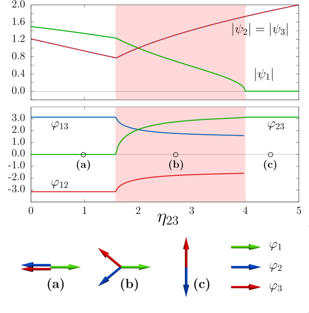
Figure 3.3: Ground state phases of the three-components superconductor (3.1), as function of $\eta_{23}$. The other parameters of the Ginzburg-Landau potential energy are $\alpha_{a}=1$, $\beta_{a}=1$, and $\eta_{12}=\eta_{13}=2$. The top graph shows the ground state densities $|\psi_{a}|$, while the bottom graph shows the relative phases $\varphi_{ab}$. All individual couplings are not simultaneously satisfied, so the system is frustrated. However, for small coupling $\eta_{23}$ (regime (a)), the relative phases are trivial (i.e. either 0 or $\pi$). For intermediate values of $\eta_{23}$ (regime (b)), all ground state relative phases are non-trivial. Hence the ground state features a discrete symmetry: $\mathrm{U}(1)\times\mathbb{Z}_{2}$ rather than $\mathrm{U}(1)$. Indeed, the energy is invariant under $\varphi_{ab}\to-\varphi_{ab}$, but the configuration cannot be continuously transformed into each other. For large Josephson coupling $\eta_{23}$ (regime (c)) the third condensate vanishes, and the only remaining relative phase is $\varphi_{12}=\pi$. The red background denotes the region of broken time-reversal symmetry. As discussed later on, the both transitions (a) $\leftrightarrow$ (b) and (b) $\leftrightarrow$ (c) are of the second order. Similar diagram showing the ground state of three-component superconductor can be found in [JG25.].

Consider, as an example, the situation where all Josephson couplings are positive. As can be seen in Table. 3.1, this situation is frustrated. The dependence of the ground state, with respect to a single Josephson coupling (here $\eta_{23}$) are displayed in Fig. 3.3. It shows three qualitatively distinct phases. At small values of $\eta_{23}$ (regime (a)), the relative phases are all trivial: $[\varphi_{12},\varphi_{13},\varphi_{23}]=[\pi,\pi,0]$. In the opposite limit, for large values of $\eta_{23}$ (regime (c)), the one condensate (here $\psi_{1}$) is fully depleted. It follows that only one of the relative phase, here $\varphi_{23}$, is relevant. The two remaining phases are $[\varphi_{2},\varphi_{3}]=[-\pi/2,\pi/2]$. The most interesting phase here is the phase (b). Indeed, as stated above, the relative phases here are neither 0 nor $\pi$. As stated above, this implies that the ground state features a discrete degeneracy, since it is not invariant under the time-reversal transformation $\mathcal{T}(\varphi_{ab})=-\varphi_{ab}$. The ground state here thus spontaneously breaks the time-reversal symmetry.

Symmetry-wise, in the phases (a) and (c), the ground state features the usual $\mathrm{U}(1)$ degeneracy associated with the global rotation of all phases. In the phase (b), on the other hand, the ground state has an extra discrete degeneracy $\mathbb{Z}_{2}$ so that the overall degeneracy is $\mathrm{U}(1)\!\times\!\mathbb{Z}_{2}$. Clearly, both phases (a) and (c) are symmetric under the time-reversal operations $\mathcal{T}(\varphi_{ab})=-\varphi_{ab}$, while the phase (b) is not. Moreover, as discussed below, the both transitions (a) $\leftrightarrow$ (b) and (b) $\leftrightarrow$ (c) are of the second order. These are thus associated with a divergent length-scale.

3.1.2 Length-scales of a three-band superconductor

The spontaneous breakdown of the time-reversal symmetry, as presented here at the phenomenological level of the Ginzburg-Landau theory, is a property of the ground state. This however also qualitatively affects the excitations, and in particular in the vicinity of the transitions of the time-reversal symmetry broken states. The detailed analysis of the length-scales and of the associated modes of the perturbation operator indeed reveals new, interesting properties. To have a grasp on this, let’s follow the procedure of the analysis of the perturbation operator described previously in Sec. 2.1. It might also be useful to compare with the analysis of the mass spectrum for single-component Ginzburg-Landau model in the section Sec: A.1 of the Appendix A. The analysis of the perturbation operator determines the mass spectrum (and thus the length-scales), and the corresponding modes. For a detailed discussion of the perturbative spectrum of three-band superconductor, see [171, 251].

Considering the perturbative expansion in terms of the infinitesimal parameter $\epsilon$

$$\psi_{a}=(u_{a}+\epsilon f_{a})\exp\left\{i\left({\bar{\varphi}}_{a}+\epsilon\frac{\phi_{a}}{u_{a}}\right)\right\}\,.$$ (3.10)

Here, $u_{a}$ and ${\bar{\varphi}}_{a}$ are respectively the ground state densities and phases, introduced in the previous section. $f_{a}\equiv f_{a}(\mathbf{x})$ are the density amplitudes, while $\phi_{a}\equiv\phi_{a}(\mathbf{x})$ are the normalized phase amplitudes. For simplicity here, we do not consider the excitations of the gauge field, and focus only on the properties of the superconducting degrees of freedom. The fluctuations are thus characterized by a system of Klein-Gordon equations for the six condensate fluctuations (three densities, plus three phases). The Klein-Gordon system reads as

$$\frac{1}{2}\Upsilon^{T}\left(-{\bm{\nabla}}^{2}+{\cal M}^{2}\right)\Upsilon\,,\leavevmode\nobreak\ \leavevmode\nobreak\ \leavevmode\nobreak\ \text{where}\leavevmode\nobreak\ \leavevmode\nobreak\ \leavevmode\nobreak\ \Upsilon=(f_{1},f_{2},f_{3},\phi_{1},\phi_{2},\phi_{3})^{T}\,.$$ (3.11)

Here ${\cal M}^{2}$ is the squared mass matrix that is straightforwardly obtained by retaining the quadratic order of the infinitesimal parameter $\epsilon$, after introducing the expansion (3.10) into the free energy (3.1). The squared mass matrix can thus be read from

$$\Upsilon^{T}{\cal M}^{2}\Upsilon=\sum_{a=1}^{3}2(\alpha_{a}+3\beta_{a}u_{a}^{2})f_{a}^{2}+\sum_{a=1}^{3}\sum_{b>a}^{3}2\eta_{ab}f_{a}f_{b}\cos{\bar{\varphi}}_{ab}$$ (3.12a)

$$+\sum_{a=1}^{3}\sum_{b>a}^{3}\frac{2\eta_{ab}}{u_{a}u_{b}}\Big{\{}(u_{a}f_{b}+f_{b}u_{a})\big{(}\phi_{b}u_{a}-\phi_{a}u_{b}\big{)}\sin{\bar{\varphi}}_{ab}-\frac{1}{2}\big{(}\phi_{b}u_{a}-\phi_{a}u_{b}\big{)}^{2}\cos{\bar{\varphi}}_{ab}\Big{\}}\,.$$ (3.12b)

The eigenspectrum of the matrix ${\cal M}^{2}$ determines the squared masses of the excitations, the associated length-scales and the corresponding normal modes.

Before quantitatively investigating the mass spectrum, important qualitative properties can be determined by carefully examining the structure of the mass matrix. As emphasized in the previous section, the current model features essentially different states, depending on whether the ground state relative phases are trivial or not.

In the case of a trivial phase-locking,

i.e. ${\bar{\varphi}}_{ab}=0,\pi$, the mass matrix (3.12) simplifies, and the density amplitudes $f_{a}$ decouple from the normalized phase amplitudes $\phi_{a}$. Indeed, since $\sin{\bar{\varphi}}_{ab}=0$ in that case, the mass matrix becomes block-diagonal (namely ${\cal M}_{f\phi}$). The mass of the density amplitudes $f_{a}$ are thus given by the eigenvalues of ${\cal M}_{ff}^{2}$ defined from

$$\Upsilon_{f}^{T}{\cal M}_{ff}^{2}\Upsilon_{f}=\sum_{a=1}^{3}2(\alpha_{a}+3\beta_{a}u_{a}^{2})f_{a}^{2}+\sum_{a=1}^{3}\sum_{b>a}^{3}2\eta_{ab}\cos{\bar{\varphi}}_{ab}f_{a}f_{b}\,.$$ (3.13)

Hence, as long as $\eta_{ab}\neq 0$, the density modes are in general mixed. It follows that, as previously discussed in Sec. 2.1, the characteristic length-scales of the density fields are associated with linear combinations of the fields, see e.g. [164, 158, 165]. This means physically that disturbing one of the density fields necessarily perturbs the others. This also implies that in a vortex, the long-range asymptotics of all density fields is governed by the same exponent, corresponding to a mixed mode with the lowest mass.

The masses of the normalized phase amplitudes $\phi_{a}$, on the other hand are given by the eigenvalues of ${\cal M}_{\phi\phi}^{2}$ defined from

$$\Upsilon_{\phi}^{T}{\cal M}_{\phi\phi}^{2}\Upsilon_{\phi}=\sum_{a=1}^{3}\sum_{b>a}^{3}\frac{-\eta_{ab}\cos{\bar{\varphi}}_{ab}}{u_{a}u_{b}}\big{(}\phi_{b}u_{a}-\phi_{a}u_{b}\big{)}^{2}\equiv-\sum_{a=1}^{3}\sum_{b>a}^{3}\eta_{ab}u_{a}u_{b}\cos{\bar{\varphi}}_{ab}\hat{\phi}_{ab}^{2}\,.$$ (3.14)

Here again, the (non-normalized) relative phase amplitudes $\hat{\phi}_{ab}:=\frac{\phi_{b}}{u_{b}}-\frac{\phi_{a}}{u_{a}}$ have been introduced, as they directly relate to the fluctuations of the relative phase. This defines again the mass of the Leggett’s mode [166].

On the other hand, for a non-trivial phase-locking,

i.e. ${\bar{\varphi}}_{ab}\neq 0,\pi$, the density fluctuation are always coupled to the phase fluctuations. Indeed, since there $\sin{\bar{\varphi}}_{ab}\neq 0$, the decoupling discuss in the previous paragraph is not possible:

$$\Upsilon^{T}{\cal M}^{2}_{f\phi}\Upsilon=\sum_{a=1}^{3}\sum_{b>a}^{3}\frac{2\eta_{ab}\sin{\bar{\varphi}}_{ab}}{u_{a}u_{b}}(u_{a}f_{b}+f_{b}u_{a})\big{(}\phi_{b}u_{a}-\phi_{a}u_{b}\big{)}\,\neq 0\,.$$ (3.15)

It follows that when the time-reversal symmetry is broken, there are no “phase-only" Leggett’s modes. Instead there appears a new kind of collective excitations where the phase difference modes are hybridized with the density (Higgs) modes [171, 215, 238, 239]. These hybridized normal modes have a complex structure that mixes all density amplitudes, to all the phase amplitudes. This is not further discussed here, and the detailed analysis of the hybridized modes can be found for example in [JG25.]. As discussed below, the hybridized modes can be associated with large characteristic length-scales even in the case of strong Josephson coupling. Note finally that, in principle, there could be accidental decouplings, but possibility this will not be discussed here. Such a possibility was discussed in a broader context of four-component models [250].

The examination of the structure of the mass matrix thus predicts important qualitative properties, especially when the time-reversal symmetry is broken. Now, for a more quantitative discussion, the eigenvalue spectrum of ${\cal M}^{2}$ has to be determined given the ground state $u_{a}$, ${\bar{\varphi}}_{ab}$. This is easily handle numerically with standard linear algebra tools. The figure 3.4 shows the various length-scales associated with the ground state displayed in Fig. 3.3, here again as functions the Josephson coupling $\eta_{23}$. The eigenspectrum of (3.11), with the (squared) mass matrix (3.12), is the set of $6$ squared masses ${\cal M}_{a}^{2}$, whose corresponding lengths $\ell_{a}=1/{\cal M}_{a}$ are the physical length scales of the model. Note again that there is a spontaneously broken $\mathrm{U}(1)$ symmetry associated with the simultaneous rotation of all phases. This mode has a zero mass, and it can easily be decoupled . Thus there are only 5 physical lengths that are associated with the superconducting condensates. The additional length-scale given by the London penetration depth, is not discussed here.

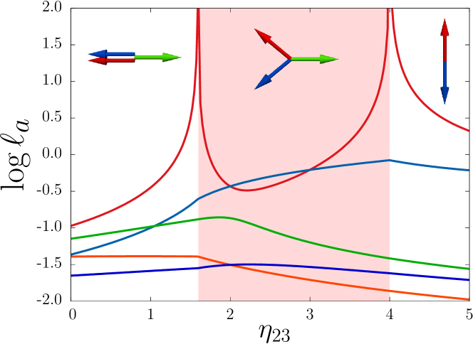
Figure 3.4: Length-scales of the three-components superconductor (3.1), as functions of the Josephson coupling $\eta_{23}$. The other parameters of the Ginzburg-Landau potential energy are $\alpha_{a}=1$, $\beta_{a}=1$, and $\eta_{12}=\eta_{13}=2$. This parameter set corresponds to the ground states displayed in Fig. 3.3. Here, the length-scale of the $\mathrm{U}(1)$ zero mode is not shown as it corresponds to an unphysical degree of freedom, so there are only 5 length-scales associated with the superconducting degrees of freedom. The penetration depth, which is not displayed here, is always finite. Here again one can clearly identify three different regimes. In the central regime, which is denoted by the red background, the time-reversal symmetry is broken, while the two other regimes are time-reversal symmetric. The transition from the time-reversal symmetric states to the time-reversal symmetry broken states is a symmetry change. It is thus expected to be accompanied by a divergent length-scale. Similar diagram showing the length-scales of three-component superconductor can be found in [JG25.]. There are also more details like the various eigenmodes.

Investigating the ground state data in Fig. 3.3, and the associated length-scales in Fig. 3.4, shows again that there are three qualitatively distinct regimes, depending on the Josephson coupling $\eta_{23}$. At $\eta_{23}=1.6$ there is a transition between the regime where with the usual $\mathrm{U}(1)$ degeneracy, and the regime where the ground state has an overall $\mathrm{U}(1)\!\times\!\mathbb{Z}_{2}$ degeneracy. A similar transition between $\mathrm{U}(1)\!\times\!\mathbb{Z}_{2}$ and $\mathrm{U}(1)$ states, occurs at $\eta_{23}=4$. As explained above, in the $\mathrm{U}(1)$ regimes, the density modes are mixed and there is no mixing between the density modes and the phase modes. It follows that the perturbations of the phases and of the densities recover independently of each other. The fluctuations of the phase modes are the three-component generalization of the standard Leggett’s modes. In the $\mathrm{U}(1)\!\times\!\mathbb{Z}_{2}$ regime all the modes are mixed, thus any perturbation of the densities induces a perturbation of the relative phases, and vice versa. At the two transition points, $\eta_{23}=1.6$ and $\eta_{23}=4$, there is a divergent length-scale. The examination of the corresponding eigenvector shows that in the $\mathrm{U}(1)$ regimes this a mode is a phase-only. Thus a Leggett mode becomes massless at the transitions to the time-reversal symmetry broken states. This was realized in the London model in [213], and in general Ginzburg-Landau model [171, 251]. It follows that here, the decay of the corresponding perturbation is not exponential, but it is governed by a power law.

The perturbation operator thus features a divergent length-scale in the vicinity of both transitions to the ${s\!+\!is}$, time-reversal symmetry breaking state. This transition is thus of the second order. Indeed, the theory of the mean-field second-order phase transitions states that the mass of one of the modes should go to zero, while other length-scales remain finite. Unlike the phase transition to the normal state, at which the gauge field becomes massless, the penetration depth is always finite at these transitions .

In the vicinity of these transition points, the largest length-scale is anomalously large due, to the frustration between Josephson couplings. Since the penetration depth remains finite, this implies that there exists always a region, close enough to the phase transition, where $\lambda$ is an intermediate length scale. It follows, as discussed in the Chapter 2, that superconductors that are in the vicinity of a time-reversal symmetry breaking transition are potentially type-1.5, with long-range attractive and short-range repulsive intervortex forces.

Time-reversal symmetry breaking in two-components superconductor

In this section, we extensively discussed how the ${s\!+\!is}$ time-reversal symmetry breaking states occur in three-component superconductors, due to the competition between the bilinear Josephson couplings. Such a three-component Ginzburg-Landau theory is relevant to describe a three-band superconducting state, with an intra-band dominated pairing (see e.g. [JG10.]). However, the ${s\!+\!is}$ state can also be realized in two-component Ginzburg–Landau models. For example, microscopic three-band model, with an interband dominated repulsive pairing were suggested to be relevant for some iron-based superconductors [220, 215, 239]. In this case, only two fields can nucleate and the relevant model is a two-component Ginzburg–Landau theory, see e.g. [JG10.]. Similar model can also be realized in dirty two-band superconductor, due to impurity scattering [252, 249, 253], see also [JG9.].

The most generic potential free energy (1) of a two-component Ginzburg–Landau model reads as:

$$V(\Psi,\Psi^{\dagger}) =\sum_{a=1}^{2}\left(\alpha_{aa}|\psi_{a}|^{2}+\frac{\beta_{aa}}{2}|\psi_{a}|^{4}\right)$$ (3.16a)

$$+2(\alpha_{12}+\gamma_{11}|\psi_{1}|^{2}+\gamma_{22}|\psi_{2}|^{2})|\psi_{1}||\psi_{2}|\cos\varphi_{12}$$ (3.16b)

$$+(\beta_{12}+\gamma_{12}\cos 2\varphi_{12})|\psi_{1}|^{2}|\psi_{2}|^{2}\,.$$ (3.16c)

This potential can describe an ${s\!+\!is}$ state, and the coefficients of the Ginzburg-Landau functional can be calculated from a given set of input microscopic parameters, from the relevant microscopic model. See for example [JG10.] for the case of a interband dominated pairing for clean superconductors, or [JG9.] and [JG5.] for dirty two-band superconductors. Note that in the ${s\!+\!is}$ case, the superconducting condensates are also coupled via mixed gradients terms $({\bm{D}}\psi_{1}^{*}{\bm{D}}\psi_{2}+c.c.)$, which do not impact the ground state. However, such terms play a role in the length scales and the associated normal modes. Details of the length scales and normal modes of such an ${s\!+\!is}$ superconducting state was investigated in [JG5.].

Here again, the potential (3.16) cannot always be minimized analytically. Yet, qualitative information can be understood by considering the different phase locking term. Indeed, the first phase-locking term (3.16b) promotes the relative phase $\varphi_{12}$ to be either $0$ or $\pi$, depending the sign of the density-dependent effective coupling $(\alpha_{12}+\gamma_{11}|\psi_{1}|^{2}+\gamma_{22}|\psi_{2}|^{2})$. The second phase-locking term, coupled via $\gamma_{12}$ in (3.16b) favors either $\varphi_{12}=\pm\pi/2$ when $\gamma_{12}>0$, or $\varphi_{12}=k\pi$ (with $k\in\mathbbm{Z}$) when $\gamma_{12}<0$. As for the three-components discussed above, the different phase-locking terms can compete with each other, and thus may lead to frustration and to a discrete degeneracy of the ground state.

The relative phase is determined by the equation $\delta V/\delta\varphi_{12}=0$:

$$\big{(}\alpha_{12}+\gamma_{11}|\psi_{1}|^{2}+\gamma_{22}|\psi_{2}|^{2}\big{)}|\psi_{1}||\psi_{2}|\sin\varphi_{12}+\gamma_{12}|\psi_{1}|^{2}|\psi_{2}|^{2}\sin 2\varphi_{12}=0\,.$$

This has different solutions in the different states:

$$s_{\pm}:\leavevmode\nobreak\ \varphi_{12}=\pi\,,\leavevmode\nobreak\ \leavevmode\nobreak\ \leavevmode\nobreak\ \leavevmode\nobreak\ s_{++}:\leavevmode\nobreak\ \varphi_{12}=0\,,\leavevmode\nobreak\ \leavevmode\nobreak\ \leavevmode\nobreak\ \leavevmode\nobreak\ s+is:\leavevmode\nobreak\ \varphi_{12}=\pm\arccos\left(-\frac{\alpha_{12}+\gamma_{11}|\psi_{1}|^{2}+\gamma_{22}|\psi_{2}|^{2}}{2\gamma_{12}|\psi_{1}||\psi_{2}|}\right)\,.$$

The ground state values of the densities are determined by the other equations $\frac{\delta V}{\delta|\psi_{a}|}=0$. The whole nonlinear system has to be solve numerically.

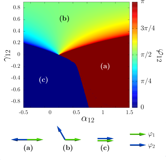
Figure 3.5: Ground state phases of the two-components superconductor, as function of linear ($\alpha_{12}$) and bilinear ($\gamma_{12}$) Josephson couplings. The other parameters of the Ginzburg-Landau potential energy are $\alpha_{aa}=-1$, $\beta_{aa}=1$, and $\beta_{12}=\gamma_{11}=\gamma_{22}=0$. The top panel shows the ground state relative phase $\varphi_{12}$. Both phase-locking cannot always be simultaneously satisfied, so the system can be frustrated. There are two phases for which the relative phase is trivial. In the regime (a) $\varphi_{12}=\pi$, while in the regime (c) $\varphi_{12}=0$ In the intermediate regime (b), the ground state relative phase is non-trivial, and the ground state features the discrete symmetry $\mathrm{U}(1)\times\mathbb{Z}_{2}$ rather than $\mathrm{U}(1)$. Similar phase diagram is found in [254, 159] where the parameters of the Ginzburg-Landau theory are expressed in terms of the parameters of the underlying microscopic theory.

For example, let’s consider the situation where the weighted Josephson couplings $\gamma_{aa}=0$, and where the biquadratic density term vanishes ($\beta_{12}=0$). The dependence of the ground state, with respect to the bilinear ($\alpha_{12}$) and biquadratic ($\gamma_{12}$) Josephson coupling is displayed in Fig. 3.5. As for the three-component model, the diagram shows three different phases: Two are time-reversal symmetric, and the time-reversal symmetry is broken in the third phase. The time-reversal symmetric states are the $s_{\pm}$ state (the red region with $\varphi_{12}=\pi$) and the $s_{++}$ state (the blue regions with $\varphi_{12}=0$).

The principal message here is that the time-reversal symmetry breaking ${s\!+\!is}$ state, that occurs in three-component models due to phase frustration, also have two-component counterpart. Here again, this is the frustrated competition between different phase-locking terms, that can result in ground states with non-trivial ground state relative phase. The principal difference is that in the case of three components, the competition between bilinear Josephson couplings is sufficient to result in frustration. On the other hand, the existence of higher order Josephson terms is necessary to obtain the frustration.

The transition between both time-reversal symmetric states can occur either via a direct crossover (directly from (a) to (c)), or via the intermediate complex ${s\!+\!is}$ state, that breaks the time-reversal symmetry (the region (b) of Fig. 3.5, where $\varphi_{12}\neq 0,\pi$). Discussions of the phase diagram of the two-component ${s\!+\!is}$ state with the relevant length scales, in terms of the parameters of the microscopic theory can be found in [JG9.], [JG5.].

Crossover region.

The direct crossover from the ${s_{\pm}}$ state (a) to the ${s_{++}}$ state (c) do not break the time-reversal symmetry. Moreover, since it is not associated with a symmetry change, there are no divergent length-scale here. Yet vortices feature interesting new properties in the vicinity of that crossover, and there is a transition in the structure of vortex cores [JG8.]. More precisely, in addition to the common singularity of both condensates, the vortices can acquire a circular nodal line around the singular point. This nodal line in one of the superconducting condensates results in a peculiar “moat"-like profile of the associated condensate. In other words, these new solutions realize the ${s_{\pm}}$ state ($\varphi_{12}=\pi$) near the vortex core, while the phase locking in the bulk is the ${s_{++}}$ state ($\varphi_{12}=0$). See the detailed discussion [JG8.]. As further discussed in [JG6.], this implies that in an external field, there can be global transitions of the overall relative phase.

Other superconducting states that break the time-reversal symmetry.

As discussed earlier, the ${s\!+\!is}$ state is the simplest time-reversal symmetry breaking extension of the most abundant $s$-wave state. There exist different superconducting states, that also break the time-reversal symmetry, as for example the ${s\!+\!id}$, ${d\!+\!id}$, or ${p\!+\!ip}$ states. All these models are described by potential similar to (3.16), and also feature domain wall excitation. However, as they may break different point group symmetries, they have essentially different kinetic terms. For example, see the different kinetic term in the two-component ${s\!+\!is}$ state features mixed gradients $({\bm{D}}\psi_{1}^{*}{\bm{D}}\psi_{2}+c.c.)$ while in the ${s\!+\!id}$ state, these are $(D_{x}\psi_{1}^{*}D_{x}\psi_{2}-D_{y}\psi_{1}^{*}D_{y}\psi_{2}+c.c.)$. As discussed later on, this can lead to different responses between these states [JG12.]. Similarly, the chiral ${p\!+\!ip}$ state also have a different structure of the kinetic term.

3.2 Topological defects in the time-reversal symmetry breaking states

The topological properties of the superconducting states that break the time-reversal symmetry where already partially addressed in Chapter 1. Indeed, in Section 1.3.3 features a heuristic description of domain-walls, and how they can pin vortices. Below, we continue with a more quantitative description of the properties of the additional topological defects in time-reversal symmetry breaking states. In particular, in relation with the underlying three-component models.

3.2.1 Domain-walls

As explained in Section 1.3.3, domain-walls are the topological defects that are naturally associated with the spontaneous breakdown of a discrete $\mathbb{Z}_{2}$ symmetry. Hence it is natural to expect that domain-walls should form in superconducting states that break the time-reversal symmetry. Following the analysis in [JG19.] these domain walls can be formed by thermal quench, and be geometrically stabilized against collapse.

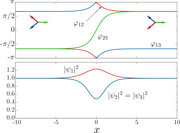
Figure 3.6: A domain-wall solution of a three-component superconductor that breaks the time-reversal symmetry. The parameters of the Ginzburg-Landau free energy (3.1) are $\alpha_{a}=0$, $\beta_{a}=1$, and $\eta_{12}=\eta_{13}=\eta_{23}=1$ and $e=0.1$. The top panel displays the relative phases, and the bottom panel shows the densities. The domains-wall interpolates between two inequivalent phase-locking. At $x=0$, the relative phases are $\varphi_{12}=\varphi_{13}=\pi$ and $\varphi_{23}=0$, thus the Josephson couplings term $\cos\varphi_{ab}$ are the most unfavourable there.

The figure 3.6 shows a domain-wall solution of a three-component Ginzburg-Landau model (3.1), when the time-reversal symmetry is broken. Here, the domain-wall interpolates between the two inequivalent ground states, with different chiralities. These solutions are found numerically by minimizing the free energy (3.1) with an appropriate initial guess. More precisely, the domain-walls interpolating between the distinct ground states fall into disjoint homotopy classes, and thus no finite energy transformation can transform it to a constant ground state (see e.g. the textbooks [1, 4, 5, 3, 8]). It follows that such an initial state is very robust to the minimization of the energy. As discussed in more details in the Section B.2.3 of Appendix B, the knowledge of the topological properties is also very useful for the numerical construction of topological defects.

It is clear from the top panel of Fig. 3.6 that the domain interpolates between the two ground states that are complex conjugate of each other. At the domain-wall, here at $x=0$, the relative phase are such that the Josephson couplings terms $|\psi_{a}||\psi_{b}|\cos\varphi_{ab}$ there are energetically the most unfavourable. As a result, the total density there is reduced, in order to reduce the energy cost.

Magnetic signature of the domain-walls:

Unlike the domain-walls that appear for example in chiral $p$-wave superconductors, the ${s\!+\!is}$ domain-walls are not associated, in principle, with a non-zero magnetic field. Indeed, the domain-walls in chiral $p$-wave superconductors, carry a uniform magnetic field due to the orbital momentum of the Cooper pairs (see e.g. [147, 148, 149], see also the discussion in [255] and detailed analysis in [256, 257]). The domain walls between the two ${s\!+\!is}$ states, on the other hand, are kinks in the relative phases. Inspection of the separation in charged and neutral modes (1.12) makes it natural to expect that the associated gradients in the relative phases do not couple to the charged modes. It is however possible, as demonstrated in [JG19.], that domain-walls between ${s\!+\!is}$ states carry a magnetic field only locally, with no net flux through the sample. Indeed, in multicomponent superconductors the relation between the magnetic field and the total current is more complicated than the usual London’s magnetostatics relation. More precisely, the magnetic field can be expressed as [JG21.], [JG19.]:

$$B_{k}=\varepsilon_{kij}\left\{\nabla_{i}\left(\frac{J_{j}}{e^{2}\varrho^{2}}\right)+\frac{i}{e\varrho^{4}}\left(\varrho^{2}\nabla_{i}\Psi^{\dagger}\nabla_{j}\Psi+(\Psi^{\dagger}\nabla_{i}\Psi)(\nabla_{j}\Psi^{\dagger}\Psi)\right)\right\}\,.$$ (3.17)

Here ${\bm{J}}$ is the total Meissner current, $\rho:=(\Psi^{\dagger}\Psi)^{1/2}$ is the total density, and $\Psi^{\dagger}=(\psi_{1}^{*},\psi_{2}^{*},\psi_{3}^{*})$ is scalar multiplet which carries all the superconducting degrees of freedom. For details of the derivation, see the related discussion in Section 1.1.3, and for generalization to anisotropic models see [258]. The first term in (3.17) is the standard contribution to the magnetic field from the superconducting currents, while the second term is the additional contribution due to the inter-component interactions. Importantly, this second term depends only on the relative phases and relative densities of the condensates. This can be seen more explicitly in the discussion about thermoelectric effects in Sec. 3.3, for example in equation (3.23). As emphasized in [JG19.], there can be situations where these additional contributions are only partially screened by the standard London contribution, thus resulting in a non-zero signature of the magnetic field.

Note that the relative phase gradients alone do not induce magnetic fields since they do not lead to charge transfer in real space. However, a magnetic field do appear if, in addition there are relative density gradients that are not collinear to the relative phase gradients. Such a local magnetic field is expected to be stronger on domain-walls, since the relative phase gradients are stronger there.

In [JG19.], it was demonstrated that such uncompensated contribution can occur if a domain-wall is attached to a boundary with an important curvature, such as "bumps" in a non-convex geometry, or pinning centres. The magnetic signatures of domain-walls, and the possibility to discriminate ${s\!+\!is}$ domain-walls with ${s\!+\!id}$ domain walls, was discussed in [259]. As further discussed in Sec. 3.3, the possibility to observe this additional contribution via thermoelectric properties was also discussed in [JG14.] and [JG12.] .

Formation of the domain-walls.

The spontaneous breakdown of the time-reversal symmetry dictates that the ${s\!+\!is}$ state possess domain wall excitations. It is well known that going through a phase transition allows uncorrelated regions to fall into different ground states [12, 13]. This is the Kibble-Zurek mechanism for the formation of topological defects. For a review of the Kibble-Zurek mechanism in conventional superconductors, see [260]. Here, while a superconductor goes through the transition to the time-reversal symmetry broken state, domain walls are created as different regions fall into either of the $\mathbb{Z}_{2}$ states [119]. Similarly, domain-walls can form in the context of chiral $p$-wave superconductors [149]. Moreover, the Kibble-Zurek mechanism relates the number of produced topological defects, with "speed" of the transition. Heuristically, a rapid transition produces more topological defects.

However, in finite systems, domain-walls can be dynamically eliminated by continuously be moved out of the domain. Nevertheless, as demonstrated in [JG19.], they can be stabilized by pinning centres. They can also be stabilized in non-convex geometries, as discussed earlier in the Section 1.3.3. The geometric stabilization, illustrated in Fig. 1.11, may help for the observability of domain-walls formed during a phase transition to the time-reversal symmetry broken states.

Furthermore, as discussed shortly, the domain-walls interact non-trivially with vortices. In a nutshell, to accommodate the unfavourable relative phase at the domain-wall, they tend to confine the vorticity. Moreover the points where the domain walls are attached to the boundaries, are easy entry points for vortices to enter the system. It follows that the magnetization process, when the zero field configuration features a stabilized domain-wall, is different than when domain-walls are initially absent [JG19.]. This can be observed via the fact the first (fractional) vortex entry occurs at much lower fields than the bulk $H_{c1}$. It can also be seen that the vortex matter distributes differently. Hence repeating measurements of the magnetization process after rapid cooling (or other kind of quench) could easily identify the presence of domain-walls, and consequently signal that the time-reversal symmetry is broken [JG19.].

3.2.2 Chiral $\mathbb{C}\mathrm{P}^{2}$ skyrmions

As mentioned above, the domain-walls interact non-trivially with vortices. It follows that, as demonstrated in [JG26.] and [JG21.], domain-walls can combine with vortices to form new kind of topological defects called chiral $\mathbb{C}\mathrm{P}^{2}$ skyrmions. The existence of such states, associated with new non-trivial topological properties, was already partially discussed in section 1.3.3. The underlying mechanisms of the interaction between domain-walls and vortices are discussed here in more details.

As previously explained, and as can be seen from the Fig. 3.6, the relative phases at the domain-wall provide the energetically most unfavourable Josephson couplings terms $|\psi_{a}||\psi_{b}|\cos\varphi_{ab}$. Moreover the domain-wall feature an additional energy cost, associated with a gradient in the relative phase $\varphi_{ab}$ in (1.12). It follows that the total density is reduced to accommodate the extra energy cost. As a results, if a vortex is close to a domain-wall, the depletion of the densities acts attractively to bind the vortex to the domain-wall. Moreover, if an integer composite vortex is located on a domain wall, the Josephson terms tend to split it into fractional vortices, thus allowing more favourable relative phase in between the split fractional vortices. In the absence of domain-walls, fractional vortices are linearly confined by the Josephson interaction terms, as discussed in the section 1.1.4 or in [JG21.]. On the other hand, domain-walls tend to confine vortices and to split them into fractional vortices that repel each other. This was discussed in details in [JG19.].

Because of its line tension, as sketched earlier in Fig. 1.10, a closed domain-wall collapses to zero size. In contrast, fractional vortices confined on a domain-wall repel each other. This opens the possibility for a composite solution consisting in a closed domain-wall ‘decorated’ with vortices to be (meta)stable. Indeed, for large enough penetration depth, the repulsion between the fractional vortices confined on the domain wall can become strong enough to overcome the domain-wall’s tension. It thus results in a composite topological defect made of $n$ fractional vortices in each condensate $|\psi_{a}|$, distributed along a closed domain-wall. Such a configuration, that carries $n$ flux quanta, is stabilized by the competing forces, see [JG26.]and [JG21.].

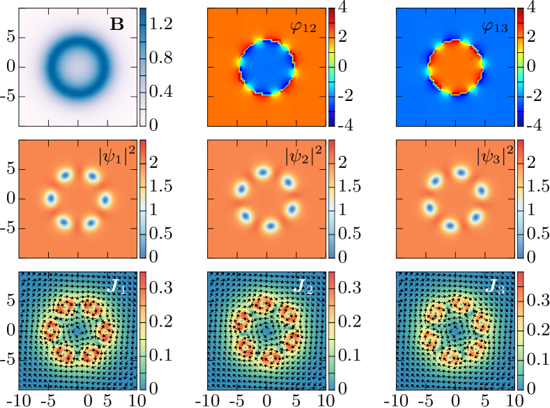
Figure 3.7: A Skyrmion solution of a three-component superconductor that breaks the time-reversal symmetry. The parameters of the Ginzburg-Landau energy (3.1), are $\alpha_{aa}=-1$, $\beta{aa}=1$ $\alpha_{ab}=1$ (with $a\neq b$), and $e=0.25$. The solution here carries six flux quanta and thus consists in 18 fractional vortices (six for each component). The displayed quantities on the top row are the magnetic field and two relative phases $\varphi_{12}$ and $\varphi_{13}$. The middle row shows the densities of the three components $|\psi_{a}|^{2}$, while the bottom row displays the associated super-currents. The flux quantization implies that these chiral skyrmions carry a topological charge (1.17) $\mathcal{Q}(\Psi)=6$.

The figure 3.7 shows the details of a composite solution consisting in $6$ fractional vortices in each of the condensates $\psi_{a}$, distributed along a closed domain-wall. As explained earlier, this numerical solution is obtained by minimizing the energy, from an initial configuration that winds $6$ times in each of the condensates (see details in Appendix B and Section B.2.3). As can be seen from the three panels showing the densities $|\psi_{a}|^{2}$, the cores of the different fractional vortices do not overlap, and thus $\Psi(\mathbf{x})\neq 0$ everywhere. It follows, as explained in details in Section 1.1.3, that these solutions are associated with a non-vanishing $\mathbb{C}\mathrm{P}^{2}$ topological invariant $\mathcal{Q}$ (1.17). The flux quantization implies that $\mathcal{Q}=6$. Hence the solution displayed in Fig. 3.7, is called a chiral $\mathbb{C}\mathrm{P}^{2}$ skyrmions of the three-component model (3.1).

Depending on the details of the model, a chiral $\mathbb{C}\mathrm{P}^{2}$ skyrmions carrying $\mathcal{Q}$ flux quanta, might be energetically favoured compared to a set of $\mathcal{Q}$ single quanta vortices [120]. In such a case, the skyrmions are expected to spontaneously form in an external field. By contrast, if the skymions are more energetic than vortices they exist as robust metastable solution. Indeed unpinning the vortices from the domain-walls is energetically costly and they are quite stable to perturbations [142, 120]. Metastable skyrmions can form in field-cooled experiments via the Kibble-Zurek mechanism, when the transition to time-reversal symmetry broken states $T_{c,\mathbb{Z}_{2}}$ occurs below the superconducting critical temperature $T_{c}$ [JG19.]. Moreover, in a finite sample a skyrmion is surrounded by regular vortices, the later press the skyrmion, thus having a stabilizing effect against its decay.

Because of the splitting of the fractional vortices, the magnetic flux is distributed along the domain wall. This can be seen in the top left panel of the figure 3.7. The choice of the parameters of the Ginzburg-Landau theory here are very symmetric, and thus flux is evenly distributed along the domain wall. When the parameters are different, then the chiral skyrmions can feature very exotic signatures of the magnetic field. This is discuss in details in [JG26.] and [JG21.]. Since they have very distinct signatures of the magnetic field, they can be observed by scanning SQUID or Hall or magnetic force microscopy experiments.

Skyrmions can also exist in other time-reversal symmetry breaking states.

As mentioned earlier, there exist superconducting states with different symmetries, that also break the time-reversal symmetry. As they also allow for domain-wall excitations, it is now rather natural to expect that they can allow for chiral skyrmions as well. As already discussed at the end of the Sec. 1.3.4, ${p\!+\!ip}$ superconductors indeed support stable skyrmionic excitations [JG23.]. Some of these can be interpreted as vortices carrying two flux quanta [JG13.], and form lattices see [JG11.] and [JG3.]. Skyrmions were also shown to have an important role in the magnetization process of mesoscopic samples of ${p\!+\!ip}$ superconductors [261, 262, 263]. For similar a discussion of skyrmions in the ${s\!+\!id}$ state, see [264].

3.3 Thermoelectric properties of superconductors that break the time-reversal symmetry

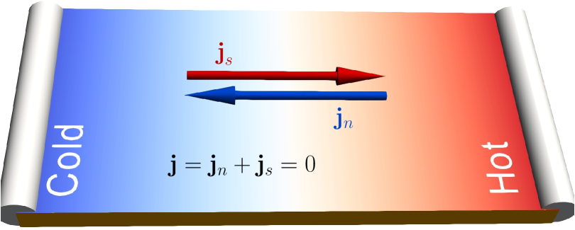
Figure 3.8: Schematic illustration of the Ginzburg mechanism for the thermoelectric effect: A temperature gradient results in a charge transfer by thermal quasiparticles, that is compensated by the counterflow of the superconducting current.

As discussed earlier, the magnetostatic properties of multi-component superconductors feature an additional contribution due to the intercomponent interactions. These extra contributions can be excited by applying thermal gradients to a multi-component superconductor, as demonstrated in [JG14.] and [JG12.].

The thermoelectric effects in superconductors, were discussed by Ginzburg in the mid 1940’s [265, 266, 267, 268]. These originate in the charge transfer by thermal quasiparticles [269], which is compensated by the counterflow of the superconducting current. Namely, a temperature gradient applied to a superconductor induces an electric current ${\bm{J}}_{n}=b_{n}{\bm{\nabla}}T$, where $b_{n}$ is the thermoelectric coefficient. This current is carried by quasiparticles that exist at finite temperatures. In superconductors, the total current also features the contribution from the superconducting electrons ${\bm{J}}_{s}$. It follows that, in contrast to a normal metal, the total current a superconductor vanishes in order to obey the Meissner effect, the thermoelectric current is cancelled by the superconducting current: ${\bm{J}}={\bm{J}}_{s}+{\bm{J}}_{n}=0$. As a result, the counterflow of the superconducting current is ${\bm{J}}_{s}=-b_{n}{\bm{\nabla}}T$. This is sketched in Fig. 3.8. In the recent years, there was a revival of the interest about this thermoelectric effect, see e.g. [270, 271, 272, 273, 274, 275].

Remark that as it is determined by the dissipative normal current, a thermally induced supercurrent is irreversible, since ${\bm{J}}_{s}$ changes its sign under the time-reversal transformation while $b_{n}$ and ${\bm{\nabla}}T$ remain invariant. As discussed below, since multicomponent superconductors feature additional contributions due to the inter-component interaction, the thermoelectric effect can be substantially altered. In particular, in superconductors that break the time-reversal symmetry [JG14.].

3.3.1 Current relations in multicomponent superconductors

It was emphasized, in Sec. 1.1.3 and in Sec. 3.2.1, that the magnetic field gets an additional contribution to the Meissner currents (see e.g. Eq.(3.17)). This extra contribution, which is due to the inter-component interactions, depends on the gradients of relative phases and relative densities. Similarly, the superconducting current features an extra contribution due to relative phase gradients. This can be seen by rewriting the current in terms of the total phase and of the relative phases. For an arbitrary number of components $N$, the individual phases can be written as

$$\varphi_{a}=\varphi_{\Sigma}+\frac{1}{N}\sum_{b\neq a}\varphi_{ab}\,,\leavevmode\nobreak\ \leavevmode\nobreak\ \text{where}\leavevmode\nobreak\ \leavevmode\nobreak\ \leavevmode\nobreak\ \varphi_{\Sigma}=\frac{1}{N}\sum_{a=1}^{N}\varphi_{a}\,,\leavevmode\nobreak\ \leavevmode\nobreak\ \text{and}\leavevmode\nobreak\ \leavevmode\nobreak\ \leavevmode\nobreak\ \varphi_{ab}:=\varphi_{b}-\varphi_{a}\,.$$ (3.18)

The total current ${\bm{J}}=e\sum_{a}|\psi_{a}|^{2}({\bm{\nabla}}\varphi_{a}+e{\bm{A}})$ thus reads as

$${\bm{J}}/e =\varrho^{2}\big{(}{\bm{\nabla}}\varphi_{\Sigma}+e{\bm{A}}\big{)}-\frac{1}{N}\sum_{a}\sum_{b\neq a}|\psi_{a}|^{2}{\bm{\nabla}}\varphi_{ab}$$ (3.19a)

$$=\varrho^{2}\big{(}{\bm{\nabla}}\varphi_{\Sigma}+e{\bm{A}}\big{)}+\frac{1}{N}\sum_{a}\sum_{b>a}\big{(}|\psi_{b}|^{2}-|\psi_{a}|^{2}\big{)}{\bm{\nabla}}\varphi_{ab}\,,$$ (3.19b)

where again $\varrho^{2}=\sum_{a}|\psi_{a}|^{2}$. Finally, introducing the notation ${\bf Q}_{\Sigma}:={\bm{\nabla}}\varphi_{\Sigma}-e{\bm{A}}$, the current reads as

$${\bm{J}}=e\varrho^{2}{\bf Q}_{\Sigma}+\frac{e}{N}\sum_{a}\sum_{b>a}\big{(}|\psi_{b}|^{2}-|\psi_{a}|^{2}\big{)}{\bm{\nabla}}\varphi_{ab}\,.$$ (3.20)

The first term here is a usual Meissner current while the second part describes the charge transfer by the counter-currents of the different superconducting condensates.

3.3.2 Thermoelectric relations in multicomponent superconductors

The key idea behind the multicomponent thermoelectric effect is that, a since the relative phases are generically temperature-dependent $\varphi_{ab}=\varphi_{ab}(T)$, a temperature bias generates a relative phase gradient between the different components. Assuming that temperature gradients are small, so that the order parameter is determined by the local temperature, the phase relation (3.18) becomes

$$\varphi_{a}=\varphi_{\Sigma}+\Gamma_{a}(T){\bm{\nabla}}T\,,\leavevmode\nobreak\ \leavevmode\nobreak\ \text{where}\leavevmode\nobreak\ \leavevmode\nobreak\ \leavevmode\nobreak\ \Gamma_{a}(T)=\frac{1}{N}\sum_{b\neq a}\frac{d\varphi_{ab}(T)}{dT}\,,$$ (3.21)

and again $\varphi_{\Sigma}=\frac{1}{N}\sum_{a=1}^{N}\varphi_{a}$. The coefficients $\Gamma_{a}(T)$ are called the thermophase coefficients. It follows that the current (3.20) can be written as

$${\bm{J}}=e\varrho^{2}\big{(}{\bf Q}_{\Sigma}+\Gamma(T){\bm{\nabla}}T\big{)}\,,\leavevmode\nobreak\ \leavevmode\nobreak\ \text{where}\leavevmode\nobreak\ \leavevmode\nobreak\ \leavevmode\nobreak\ \Gamma(T)=\sum_{a}\frac{|\psi_{a}(T)|^{2}}{N\varrho(T)^{2}}\Gamma_{a}(T)\,.$$ (3.22)

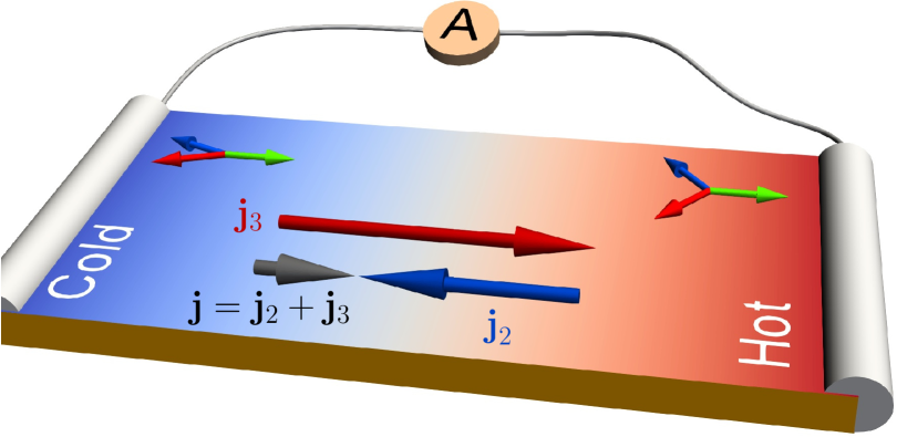
Figure 3.9: A superconducting sample subject to thermal gradients. The thermophase effect appears because of the temperature-dependent intercomponent relative phase $\varphi_{ab}=\varphi_{ab}(T)$. In the case of a superconducting state that breaks the time-reversal symmetry, the total thermally induced current ${\bm{J}}$ will have opposite directions for different TRSB states.

Note that the thermophase coefficients are odd under the time-reversal transformation: ${\cal T}(\Gamma_{a})=-\Gamma_{a}$. This implies that, in a superconductor that breaks the time-reversal symmetry, the thermophase coefficients are opposite for the different ${s\!+\!is}$ states. Thus the thermally induced superconducting currents are sensitive to the time-reversal transformation. Hence, given a temperature bias, the currents flow in opposite directions for the different time-reversal symmetry broken states [JG14.]. This is sketched in Fig. 3.9.

As demonstrated in [JG14.], the thermophase coefficients can be large in the vicinity of the time-reversal symmetry breaking transition $T_{\mathbb{Z}_{2}}$. Moreover, the discussed thermoelectric effect generically dominates at low temperatures in the ${s\!+\!is}$ state. More precisely the new contribution is important in the vicinity of the time-reversal symmetry breaking phase transition $T_{\mathbb{Z}_{2}}$, which can occur at much lower temperature than $T_{c}$. There, the usual contribution to the Ginzburg mechanism due to the thermal quasiparticles is typically extinct.

3.3.3 Magnetic and electric fields induced due to thermal gradients

Similarly to the total current (3.20), the magnetic field ${\bm{B}}$ features additional contributions as already demonstrated in (3.17) (see also the corresponding discussion in Sec. 1.1.3). Using the notations of (3.19) and (3.20), the magnetic field reads as

$${\bm{B}}={\bm{\nabla}}\!\times\!\left(\frac{{\bm{J}}}{e^{2}\varrho^{2}}\right)-{\bm{\nabla}}\!\times\!{\bm{\nabla}}\varphi_{\Sigma}+\sum_{a}\sum_{b>a}{\bm{\nabla}}\!\times\!\left(\frac{|\psi_{a}|^{2}-|\psi_{b}|^{2}}{Ne\varrho^{2}}{\bm{\nabla}}\varphi_{ab}\right)\,.$$ (3.23)

Here again, the first term is the contribution of the Meissner currents and the second term is the contribution of the total vorticity. Finally, the most interesting new contribution is the last term.

In the absence of phase windings, then the equation (3.23) can further be simplified. Indeed, when none of the phase has a singularity then all ${\bm{\nabla}}\!\times\!{\bm{\nabla}}\varphi\equiv 0$, and the magnetic field reads as

$${\bm{B}}={\bm{\nabla}}\!\times\!\left(\frac{{\bm{J}}}{e^{2}\varrho^{2}}\right)+\sum_{a}\sum_{b>a}{\bm{\nabla}}\left(\frac{|\psi_{a}|^{2}-|\psi_{b}|^{2}}{Ne\varrho^{2}}\right)\times{\bm{\nabla}}\varphi_{ab}\leavevmode\nobreak\ \leavevmode\nobreak\ \leavevmode\nobreak\ \leavevmode\nobreak\ \leavevmode\nobreak\ \text{if}\leavevmode\nobreak\ \leavevmode\nobreak\ \oint{\bm{\nabla}}\varphi_{a}\!\cdot d{\bm{\ell}}=0\leavevmode\nobreak\ \leavevmode\nobreak\ \forall a\,.$$ (3.24)

It is clear from there, that when the relative density gradients are collinear with the relative phase gradients, then there are no new contributions to the magnetic field. The most interesting situation is when they are perpendicular. The additional contribution can be screened only partially and thus leads to non-trivial signatures of the magnetic field (3.24). As discussed below, there are various situations to take advantage of this, to highlight new properties of the ${s\!+\!is}$ state.

As already repeated on various occasions the time-reversal symmetry breaking ${s\!+\!is}$ state feature domain wall excitations. It is known that such domain walls do not carry magnetic field at constant temperature [119]. Clearly, the relative phase gradients, are the most important, where the domain is located. So intuitively this is a good starting point for searching the extra contribution to the magnetic field of (3.24). One way to impose relative density variations is to apply a temperature gradient along the domain wall. For example, the temperature dependence of the coefficients of the quadratic term of the Ginzburg-Landau theory can be modelled as $\alpha_{aa}\propto\left[T(\mathbf{x})/T_{c,a}-1\right]$ ($T_{c,a}$ being a characteristic constant). There, the thermophase coefficients $\Gamma(T)$ have opposite signs in the $s+is/s-is$ domains. Therefore, in the vicinity of the interface between these, there should be a net superconducting current and a thermally induced magnetic field ${\bm{B}}$ (3.24). Such a local modification of the parameters was demonstrated to be responsible for the existence of spontaneous magnetic field in different models time-reversal symmetry breaking states, in various situations. These include the responses to linear thermal gradients [JG14.] and [JG1.], hotspot created by a laser pulse [JG12.], or [276], but also the effect of impurities [216, 277], and other inhomogeneous arrays [JG5.], [278].

Multicomponent superconductors are characterized by additional intercomponent contributions, not only to the magnetic field, but also to the electric field ${\bm{E}}=-\partial_{t}{{\bm{A}}}-{\bm{\nabla}}{\bm{A}}_{0}$. This can be seen by similar procedure that when rewriting ${\bm{B}}$, or by combining Eq.(3.24) to Faraday’s law. The electric field thus reads as

$${\bm{E}}=\partial_{t}\left(\frac{{\bm{J}}}{e^{2}\varrho^{2}}\right)+\sum_{a}\sum_{b>a}\partial_{t}\left(\frac{|\psi_{b}|^{2}-|\psi_{a}|^{2}}{Ne\varrho^{2}}{\bm{\nabla}}\varphi_{ab}\right)-{\bm{\nabla}}\Phi\leavevmode\nobreak\ \leavevmode\nobreak\ \leavevmode\nobreak\ \leavevmode\nobreak\ \text{where}\leavevmode\nobreak\ \leavevmode\nobreak\ \Phi=A_{0}-\partial_{t}\varphi_{\Sigma}\,.$$ (3.25)

Here, the gauge invariant potential field $\Phi$ is determined by the sum of chemical potential differences between the quasiparticles $\mu_{q}=e{\bm{A}}_{0}$ and each of the condensates $\mu^{(a)}_{p}=-\partial_{t}\varphi_{a}/N$. Each of the partial potential differences $\Phi^{(a)}=[\mu_{q}-\mu^{(a)}_{p}]/e$ is proportional to charge imbalance in the $a$-th band $Q^{*}_{a}=2e^{2}\nu_{0}\Phi^{(a)}$ where $\nu_{0}$ is the density of states [279, 280, 281].

Thus, as for the magnetic field, the electric field feature a contribution from the intercomponent interactions. As discussed in details in [JG12.], this additional contribution can be used to probe the properties of superconducting states that break the time-reversal symmetry. In particular by measuring the nonequilibrium electric responses generated by nonstationary heating when the local temperature evolves, recovering from the initial hot spot created, e.g. , by a laser pulse [282, 246, 276]. More precisely, in a multicomponent system, a charge imbalance can be generated by the spatial and temporal variations of the intercomponent relative phase. This originates in a nonequilibrium redistribution of the Cooper pairs between the different components, and thus creates an imbalance of partial charge $Q^{*}_{a}$. The generated charge imbalance can be measured using the normal metal and superconducting potential probes [283, 284].

Similarly to the spontaneous magnetic field, the induced charge imbalances are sensitive to the broken time-reversal symmetry. Indeed, for the same heating protocol, the degenerate $s\!+\!is$ and $s\!-\!is$ states produce opposite electric fields and charge imbalances. It is thus possible to discriminate between the usual thermoelectric response occurring in conventional superconductors, and the unconventional response that signals states that break the time-reversal symmetry. Moreover, the responses are also sensitive to the pairing symmetry, and can for example differentiate the ${s\!+\!is}$ from the ${s\!+\!id}$ state [JG12.].

Overview and Perspectives

Overview

This report tried to convey the message that multicomponent models, and in particular multicomponent superconductors, host a very rich physics that is absent in their single-component counterparts.

As emphasized in the introduction, the topological excitations are ubiquitous in physics, as they appear for example in solid state physics, condensed and soft matter systems, high-energy physics, and more. Depending on the associated topological properties, these kind of objects have different structure. They can be particle-like, point-like, "wall"-like, or line-like. In the later case, the topological defects are termed vortices, and they have been extensively studied in the context of superfluidity and superconductivity. Vortices can determine to a large extent the thermodynamic, electric and magnetic properties of the considered materials. The choice of the narrative in the introduction tries to emphasize that vortices attracted a lot of attention for a long time, and that some old concepts are still relevant in modern physics.

Because of the larger number of degrees of freedom, the multicomponent models of superconductivity allow for a rich spectrum of topological defects. The first chapter was essentially dedicated to formalize the topological properties of the multicomponent superconductors. It was further discussed various contributions of the author, in the construction of new kind of topological defects in different models of multicomponent superconductivity. These new topological defects may be used to identify properties of the underlying models. Moreover, it was emphasized in the second chapter, that multicomponent superconductors not only host new kind of topological excitations, but also that they can interact differently than the usual vortices. This new interaction between the vortices is essentially different from that of type-1 or type-2 single-component superconductors. It follows that vortices can form aggregates, and this have important impact on the various observable physical processes. Finally, there can also exist superconducting states that break the time-reversal symmetry, because of the competition between different pairing channels. These states are associated with new effects that can be measured, as discussed in the last chapter.

It is important to stress again that all the author’s contributions rely on an intensive use of numerical techniques. The numerical aspects are quite often disregarded, in favour of the discussions of the physical properties. It seemed important to take the opportunity of this report, to present in more details these numerical aspects.

All the results discussed in this report seek to emphasize the richness of the physics of multicomponent system. This is just the tip of the iceberg, and many more can be said. Despite the physics of topological defects is quite an old story now, there is still a lot to be discovered.

Perspectives

As it was emphasized in the report, there is a growing number of known multiband/multicomponent superconducting materials. Hence this is an always evolving playground to look for new relevant theories, and to investigate their topological properties. So in some sense, there are always unknown projects that may be worth investigating because of their relevance to new materials. In any case, many aspects of models of multicomponent superconductors are probably still to be discovered. Below, we can present three promising directions in relations with the aspects discussed in the report.

Project 1: Anomalous superconducting states that break the time-reversal symmetry.

Some of the new properties of the ${s\!+\!is}$ state, which spontaneously breaks the time-reversal symmetry, were reported in details in this report. These include, among other things, the existence of collective modes which includes massless [213] and mixed phase-density [171, 238, 215, 239] excitations, unconventional mechanism of vortex viscosity [240], formation of vortex clusters [171], unconventional contribution to the thermoelectric effect [245, 246]. The ${s\!+\!is}$ state is also predicted to host topological excitations such as skyrmions and domain walls [142, 120, 119].

Recently, the specific heat measurement in hole-doped Ba_1-xK_xFe₂As₂, at doping $x\approx 0.8$ showed an intriguing behaviour [285]. Namely, the spontaneous Nernst effect and muon spin rotation experiments indicates a state in which the Cooper pairs are incoherent, but which spontaneously breaks time-reversal symmetry. When a multicomponent superconductors breaks the time-reversal symmetry, there can be multiple phase transitions. At the level of the mean-field theory, the superconducting phase transition $T_{c}$ always occurs at a temperature equal to or higher than the transition temperature of the broken time-reversal symmetry $T_{\mathbb{Z}_{2}}$. The recent results show an opposite behaviour where $T_{\mathbb{Z}_{2}}>T_{c}$ [285]. All the discussion about the role of the fluctuations, and the implications are beyond the discussions here. Yet a few remarks on the structure of the model opens interesting perspectives.

As discussed in this report, multi-component superconductor feature an additional contribution to the magnetic field because of the inter-component interactions (3.17). Then, the Ginzburg-Landau free energy expressed in terms of charged and neutral modes (1.12) can further be written as

$$\mathcal{F}=\frac{1}{2}\left[\varepsilon_{kij}\left\{\nabla_{i}\left(\frac{J_{j}}{e^{2}\varrho^{2}}\right)+\frac{i}{e\varrho^{4}}{\cal Z}_{ij}\right\}\right]^{2}+\frac{{\bm{J}}^{2}}{2e^{2}\varrho^{2}}+{\bm{\nabla}}\Psi^{\dagger}\!\cdot\!{\bm{\nabla}}\Psi+\frac{1}{4\varrho^{2}}\big{(}\Psi^{\dagger}{\bm{\nabla}}\Psi-{\bm{\nabla}}\Psi^{\dagger}\Psi\big{)}^{2}+V(\Psi)\,,$$

$$\leavevmode\nobreak\ \leavevmode\nobreak\ \leavevmode\nobreak\ \leavevmode\nobreak\ \leavevmode\nobreak\ \text{where}\leavevmode\nobreak\ \leavevmode\nobreak\ \leavevmode\nobreak\ {\cal Z}_{ij}=\varrho^{2}{\bm{\nabla}}_{i}\Psi^{\dagger}{\bm{\nabla}}_{j}\Psi+(\Psi^{\dagger}{\bm{\nabla}}_{i}\Psi)({\bm{\nabla}}_{j}\Psi^{\dagger}\Psi)\,.$$ (3.26)

In the anomalous state, the superconducting part of the model is disordered, and the part corresponding to London screening is absent, that is ${\bm{J}}=0$. Then an effective model for the new state, can be derived from (Project 1: Anomalous superconducting states that break the time-reversal symmetry.), with requiring that the superconducting current vanish ${\bm{J}}=0$. This amount to retain only the degrees of freedom that are related to relative phases. The corresponding model thus reads as [285]

$$\mathcal{F}=\frac{1}{2}\left[\frac{i\varepsilon_{kij}}{e\varrho^{4}}{\cal Z}_{ij}\right]^{2}+{\bm{\nabla}}\Psi^{\dagger}\!\cdot\!{\bm{\nabla}}\Psi+\frac{1}{4\varrho^{2}}\big{(}\Psi^{\dagger}{\bm{\nabla}}\Psi-{\bm{\nabla}}\Psi^{\dagger}\Psi\big{)}^{2}+V(\Psi)\,.$$ (3.27)

As discussed in details in [285], the effective theory for the anomalous normal state, which breaks the time-reversal symmetry, allows for domain walls excitations. These feature magnetic signatures, as those discussed in the main body in the Chapter 3.

This new effective model offers lot of new opportunity to observe unusual properties of multi-component models in an anomalous state. That is, there is an opportunity to observe some of the topological properties of multi-component superconductors, above the critical temperature. Of course here, the model (3.27) is obtained heuristically, and a careful derivation is required to properly handle how the different terms should be renormalized, when the superconducting part of the model is disordered.

Project 2: Other superconducting states that break the time-reversal symmetry.

Not only the number of known multiband/multicomponent superconductors is growing, but also of those that break the time-reversal symmetry [286]. It was emphasized in this report that the superconducting states which spontaneously break the time-reversal symmetry feature new properties. Most of the focus was on the ${s\!+\!is}$ state, which is highly relevant for iron based superconductors. Another very investigated time-reversal symmetry breaking state, is the ${p\!+\!ip}$ in relations with spin-triplet superconducting models. There are various other superconducting states, which break the time-reversal symmetry, but with other pairing symmetries, e.g. ${s\!+\!id}$, ${d\!+\!id}$. Also for example, it was recently argued that the pairing in Sr₂RuO₄ could be either ${d\!+\!id}$ or $d\!+\!ig$ [287, 288]. These states that are different from ${p\!+\!ip}$ or ${s\!+\!is}$, are much less studied, and in particular their topological properties.

Since they break the time-reversal symmetry, all these states should feature domain-wall excitations as well. However, the difference is that they break different point group symmetries. At the level of the Ginzburg-Landau model, this manifests by having different, more rich structure of the kinetic terms in the form of anisotropies and mixed gradients. Like for example $(D_{x}\psi_{1}^{*}D_{x}\psi_{2}-D_{y}\psi_{1}^{*}D_{y}\psi_{2}+c.c.)$ for the ${s\!+\!id}$ state which breaks the $C_{4}$ symmetry. Or for example the $d+id$ state, which violates both parity and time-reversal symmetries [208, 235] .

The peculiarities of these other pairing symmetries, have been much less studied. For example because of their different structures, they should also manifest thermoelectric responses qualitatively different from those discussed in the Chapter 3. Moreover, the structure of the topological defect should also definitely be sensitive to that.

Project 3: Knots and vortons in the electroweak theory.

The idea here, is to look for topological defects in a theory different than that describing multi-component superconductivity. More precisely, the goal is to investigate the possibility that the Weinberg-Salam theory of the electroweak interactions could host topological defect with a knotted structure.

As emphasized in the introduction, the idea of knotted vortices is an old story that received a new breath after knotted topological defects were constructed in the Skyrme-Faddeev model [38]. Since that, there was a lot of activity in tracking similar object in various physical systems as for example in spinor Bose-Einstein condensates [289], optical beams [290], nematic colloids [291], magnetic materials [292, 293], and more; for a review on knots, see [43].

Vortons are objects that, although formally different, are quite alike to knotted vortices. These are closed loops of superconducting vortices [32], that are expected to be stabilized against contraction by the centrifugal force produced by the current [294]. They are expected to occur in a model first introduced by Witten [32], which a two-component model but with two abelian gauge fields (instead of one for superconductors). The explicit construction of vorton, and the demonstration of their potential stability is however rather recent [43, 295, 296, 297].

The bosonic sector of the Weinberg-Salam theory of the electroweak interactions, can be seen, to some extent, as a multi-component theory but more involved than those discussed in this report. Indeed, it is a theory of a doublet of complex scalars (the Higgs field). But the gauge sector is more complicated, as also contains a non-Abelian $\mathrm{SU}(2)$ gauge field, in addition to the $\mathrm{U}(1)$ gauge field. It is usually assumed that the electroweak theory admits no solitons, however there are indications that it might host some kind of vortons, or knotted vortices. Not only the theory allows for vortices, but also in some limiting cases, it can be very similar to the model of Witten where vortons exist.

Strictly speaking the electroweak theory is different than the models of multicomponent superconductivity models discussed in the main body of the report. Yet since they share some properties. One could imagine that this theory supports knotted vortex solutions similar to those obtained in the framework of two-component superconductors with dissipationless Andreev-Bashkin drag interaction [JG4.]. If such electroweak vortons or knotted vortices exist, this could be of scientific value.

Appendices

Appendix A Single-component Ginzburg-Landau theory

The main body of this report presents results regarding the properties of the theories of superconductivity featuring multiple order parameters or order parameters with multiple components. It might be useful, for a better understanding of the peculiarities of multicomponent theories, to review the essential properties of of the conventional, single-component, models of superconductivity. Covering all the microscopic aspects of conventional superconductivity is well beyond the scope of the present discussions, and these will not be discussed here. Both microscopic, and mean field aspects of single-component superconductivity are extensively discussed in a great number of classical textbooks, see e.g. [298, 73, 163, 299, 300, 301, 302, 303, 304, 305].

Hence the present background review is restricted only to the classical mean-field aspects of superconductivity. More precisely, this Appendix presents the general theoretical framework, and the textbook properties of the single-component Ginzburg-Landau theory.

The Ginzburg-Landau theory [150] was introduced in 1950, to account for the properties of the superconducting state. This phenomenological theory is based on the Landau theory of theh second order phase transitions, where the (macroscopic) order parameter $\psi=|\psi|\mathrm{e}^{i\varphi}$, is a complex scalar field. The order parameter $\psi$ is often equivalently termed superconducting condensate. The microscopic Bardeen-Cooper-Schrieffer theory of superconductivity [70] was derived later in 1957. Shortly after, in 1959 Gor’kov demonstrated that the Ginzburg-Landau theory can be derived as classical approximation of the microscopic theory [72], and the modulus of the order parameters $\psi$ is actually the density of Cooper pairs: $n_{s}=|\psi|^{2}$. Strictly speaking, the Ginzburg-Landau theory is valid only in a close vicinity of the critical temperature $T_{c}$ where the superconductivity is destroyed, and it assumes that $\psi$ is small and is slowly varying (small gradients).

Remark that besides its fundamental applications in solid state physics, the Ginzburg-Landau theory attracted a lot of attention in the mathematical community from the 1990’s, after the report of the well posedness of the problem [77, 306, 78, 307]. Since these earlier works, there have been a big activity in understanding the mathematical properties of that problem, see for example [79]. In parallel there also have been continuous efforts in the physics community to have optimal formulation for numerical solvers, see for example [308, 309].

In the vicinity of the critical temperature, the superconducting state is governed by the Ginzburg-Landau free energy, whose density reads as [150] (see textbook discussions, e.g., [73, 163]):

$$\mathcal{F}=\alpha|\psi|^{2}+\frac{\beta}{2}|\psi|^{4}+\frac{1}{2m_{\star}}\left|\left(\frac{\hbar}{i}{\bm{\nabla}}-\frac{e_{\star}}{c}{\bm{A}}\right)\psi\right|^{2}+\frac{{\bm{B}}^{2}}{8\pi}.$$ (A.1)

Here $e_{\star}$ and $m_{\star}$ are respectively the effective charge and mass of the Cooper pairs, $\hbar$ is the reduced Planck’s constant and $c$ is the speed of light. For a consistency with the text of the main body of the report, it is convenient to consider the Ginzburg-Landau free energy $F=\int d^{3}\mathbf{x}\,\mathcal{F}$, whose density (in conveniently chosen dimensionless units) reads as

$$\mathcal{F}=\frac{{\bm{B}}^{2}}{2}+\frac{1}{2}\left|\left({\bm{\nabla}}+ie{\bm{A}}\right)\psi\right|^{2}+\alpha|\psi|^{2}+\frac{\beta}{2}|\psi|^{4}\,.$$ (A.2)

Since $\psi$ is a charged scalar field, it is coupled to ${\bm{A}}$, the vector potential of the magnetic field ${\bm{B}}={\bm{\nabla}}\!\times\!{\bm{A}}$, via the gauge derivative ${\bm{D}}\equiv\left({\bm{\nabla}}+ie{\bm{A}}\right)$. $e$ is a coupling constant sometimes called the gauge coupling constant. For the energy to be bounded from below, the parameter $\beta$ must be positive, while $\alpha$ is either positive or negative. In the presence of an external applied field ${\bm{H}}_{e}$, this is the Gibbs free energy,

$$G=F-\int{\bm{B}}\cdot{\bm{H}}_{e}\,,$$ (A.3)

that should be considered instead of the Helmholtz free energy $F$. The Ginzburg-Landau theory (A.2) is thus as classical field theory, where the physical degrees of freedom are a complex scalar field $\psi(\mathbf{x})$ standing for the superconducting condensate and the gauge field ${\bm{A}}(\mathbf{x})$ (the vector potential), a real vector field.

The functional variation of the Ginzburg-Landau functional (A.2) with respect to $\psi^{*}$ gives the Ginzburg-Landau equation

$${\bm{D}}{\bm{D}}\psi=2\left(\alpha+\beta|\psi|^{2}\right)\psi\leavevmode\nobreak\ \leavevmode\nobreak\ \leavevmode\nobreak\ \leavevmode\nobreak\ \text{with}\leavevmode\nobreak\ \leavevmode\nobreak\ \leavevmode\nobreak\ {\bm{D}}\equiv\left({\bm{\nabla}}+ie{\bm{A}}\right)\,,$$ (A.4)

while the variations with respect to the vector potential ${\bm{A}}$ yield the Ampère-Maxwell equation

$${\bm{\nabla}}\!\times\!{\bm{B}}+{\bm{J}}=0\,,\leavevmode\nobreak\ \leavevmode\nobreak\ \leavevmode\nobreak\ \leavevmode\nobreak\ \text{with}\leavevmode\nobreak\ \leavevmode\nobreak\ \leavevmode\nobreak\ {\bm{J}}=e\mathrm{Im}(\psi^{*}{\bm{D}}\psi)=e|\psi|^{2}({\bm{\nabla}}\varphi+e{\bm{A}})\,.$$ (A.5)

The right-hand side of the Ampère-Maxwell equation, ${\bm{J}}$, is termed superconducting current or supercurrent. The Ginzburg-Landau equation (A.4) together with the Ampère-Maxwell equation (A.5) are the Euler-Lagrange equations of motion of the Ginzburg-Landau theory (A.2).

Both the superconducting condensate $\psi$ and the gauge field satisfy the boundary conditions that represent the physical properties of the system. The conditions on a Superconductor/Insulator interface $\partial\Omega_{SI}$ are

$${\bm{D}}\psi\cdot{\bm{n}}=0\,,\leavevmode\nobreak\ \leavevmode\nobreak\ ({\bm{\nabla}}\!\times\!{\bm{A}})\times{\bf n}={\bm{H}}_{e}\times{\bf n}\,,$$ (A.6)

while the Superconductor/Normal metal interface $\partial\Omega_{SN}$ is described by

$${\bm{D}}\psi\cdot{\bm{n}}=i\gamma\psi\,,\leavevmode\nobreak\ \leavevmode\nobreak\ ({\bm{\nabla}}\!\times\!{\bm{A}})\times{\bf n}={\bm{H}}_{e}\times{\bf n}\,.$$ (A.7)

The real parameter $\gamma$ depends on the details of the materials. Here, ${\bf n}$ is the outgoing normal vector to the interface. In all generality, the overall boundary $\partial\Omega$ is thus defined as $\partial\Omega=\partial\Omega_{SI}\cup\partial\Omega_{SN}$.

Gauge invariance

The theory is well known to be invariant under the local transformations generated by the elements having value in the Lie algebra of the $\mathrm{U}(1)$ gauge group (see, e.g. [73, 163]). The spontaneous breakdown of that symmetry is responsible for the longitudinal component of the photon to become massive and then being effectively a massive vector (Proca) field. In other words, in the Meissner state the gauge field is massive with an exponential decay to due the screening currents. The $\mathrm{U}(1)$ transformations $\mathcal{G}_{\chi}$ that are symmetries of the free energy (A.2), of the Ginzburg-Landau (A.4) and of the Ampère-Maxwell (A.5) equations are

$$\mathcal{G}_{\chi}:(\psi,{\bm{A}})\longmapsto\left(\psi\mathrm{e}^{i\chi},{\bm{A}}-\frac{1}{e}{\bm{\nabla}}\chi\right)\,,$$ (A.8)

for any (sufficiently smooth) real-valued function $\chi:=\chi(t,\mathbf{x})$. The observable physical quantities such as ${\bm{B}}$, ${\bm{J}}$, $|\psi|$, etc are invariant under these gauge transformations (A.8). Obviously any choice of the gauge function $\chi(t,\mathbf{x})$ that preserves the boundary behaviour (A.6) and (A.7) is physically valid, since it does not affect the physical observables. However, it is important to note that different choices of gauge do lead to different mathematical structures of the system. This is well known that some structures are easier to analyse, for example numerically, than some others (see detailed discussions in, e.g. , [78, 306, 310, 311, 312, 313].

Dynamics

The Ginzburg-Landau energy describes the magnetostatic properties of superconductors. Their dynamics is described by the time-dependent Ginzburg-Landau equations [314, 315, 316]. In the dimensionful units of Eq.(A.1), the time-dependent Ginzburg-Landau equations reads as

$$\frac{\hbar^{2}}{2m_{\star}D}\left(\partial_{t}+\frac{ie_{\star}}{\hbar}A_{t}\right)\psi +\frac{1}{2m_{\star}}\left(\frac{\hbar}{i}{\bm{\nabla}}-\frac{e_{\star}}{c}{\bm{A}}\right)^{2}\psi+\big{(}\alpha+\beta|\psi|^{2}\big{)}\psi=0\,,$$ (A.9a)

$${\bm{\nabla}}\!\times\!{\bm{\nabla}}\!\times\!{\bm{A}} =-\frac{4\pi\sigma}{c}\left(\frac{1}{c}\partial_{t}{\bm{A}}+{\bm{\nabla}}A_{t}\right)+\frac{4\pi}{c}{\bm{J}}_{s}+{\bm{\nabla}}\!\times\!{\bm{H}}_{e}\,.$$ (A.9b)

Here, $\sigma$ is the normal state conductivity and $D$ is a diffusion constant. $A_{t}$ is the electrostatic potential, ${\bm{H}}_{e}$ stands for an externally applied field and ${\bm{J}}_{s}$ is the supercurrent that reads as:

$${\bm{J}}_{s}=\frac{e_{\star}\hbar}{m_{\star}}\left(\mathrm{Im}\left(\psi^{*}{\bm{\nabla}}\psi\right)-\frac{e_{\star}}{\hbar c}|\psi|^{2}{\bm{A}}\right)\,.$$ (A.10)

Up to the $\frac{4\pi}{c}$ factor, the left hand side of Eq.(A.9b) is the total current being the superposition of superconducting and normal currents: ${\bm{J}}={\bm{J}}_{n}+{\bm{J}}_{s}$. Indeed the normal current satisfies Ohm’s law (${\bm{J}}_{n}=\sigma{\bm{E}}$), and according to Faraday’s law the electric field is ${\bm{E}}=-\frac{1}{c}\partial_{t}{\bm{A}}-{\bm{\nabla}}A_{t}$. As a result Eq.(A.9b), in absence of an external field ${\bm{H}}_{e}$, is the Ampère’s law: ${\bm{\nabla}}\!\times\!{\bm{B}}=\frac{4\pi}{c}{\bm{J}}$.

It is important to emphasize the dissipative nature of the time-dependent Ginzburg-Landau equations. Indeed, the time-dependent equation (A.9), can be understood as a gradient flow of the free energy (A.1). This implies in particular that the time evolutions leads to stationary solutions, that are (local) minima of the free energy (A.9). For rigorous demonstration of that statement, see [77, 306, 78, 307, 79].

The next discussions are only about the stationary properties of the Ginzburg-Landau theory. Hence it is convenient to re-introduce the dimensionless units of Eq. (A.2).

Relativistic version: the Abelian-Higgs Model

The Ginzburg-Landau model is very similar to the Abelian-Higgs Model that has been extensively studied in the framework of high-energy physics. Indeed, this is the theory of a complex scalar field charged under the $\mathrm{U}(1)$ gauge group of electromagnetism. In that framework, the scalar field $\psi$ is the Higgs field, and the gauge field is the four-potential of the electromagnetic field $(A_{t},{\bm{A}})$ . The energy in the Abelian-Higgs model, which reads as

$$E=\bigintsss d^{4}{\rm x}\left\{\frac{1}{2}({\bm{E}}^{2}+{\bm{B}}^{2})+|D_{t}\psi|^{2}+|{\bm{D}}\psi|^{2}+\frac{\beta}{8}(|\psi|^{2}-1)^{2}\right\}\,,$$ (A.11)

is very similar to that of the Ginzburg-Landau theory. Again, the gauge derivative is $D_{\mu}\psi=(\partial_{\mu}+ieA_{\mu})\psi$. The constant $\beta$ is the self-interacting constant of the scalar field, and it is similar to the Ginzburg-Landau parameter $\kappa$ introduced below.

The close similarity between both models, implies that they share the same static solutions. However, it is important to stress that the dynamics is very different. Indeed, while the dynamics in the Abelian-Higgs model is relativistic, the dynamics of superconductors is determined by the time-dependent Ginzburg-Landau equations (A.9). As discussed above, the latter is a dissipative equation, while the dynamics of the Abelian-Higgs model is “wave-like".

A.1 Ground state, Length-scales and the Meissner effect

Superconducting ground state

The ground state is, by definition, the state which gives the minimal value of the energy. Since the magnetic and kinetic energy contributions are quadratic, the minimum of the energy satisfies

$$\left\{\begin{array}[]{c}{\bm{\nabla}}\!\times\!{\bm{A}}=0\\ ({\bm{\nabla}}+ie{\bm{A}})\psi=0\end{array}\right.\leavevmode\nobreak\ \leavevmode\nobreak\ \leavevmode\nobreak\ \text{whose general solutions are}\leavevmode\nobreak\ \leavevmode\nobreak\ \leavevmode\nobreak\ \left\{\begin{array}[]{c}{\bm{A}}={\bm{\nabla}}\chi(\mathbf{x})\\ \psi=\mathrm{const.}\times\mathrm{e}^{ie\chi(\mathbf{x})}\end{array}\right.\,,$$ (A.12)

for an arbitrary regular function $\chi(\mathbf{x})$. The solutions (A.12) are easily identified with the gauge transformations (A.8). It is thus straightforward to choose the simplest solution ${\bm{A}}=0$ and $\psi=\text{constant}$, that simultaneously minimize both magnetic and kinetic contributions in the free energy. It follows that the minimal energy configuration corresponds to the minimum of the potential energy

$$V(\psi)=\alpha|\psi|^{2}+\frac{\beta}{2}|\psi|^{4}\,.$$ (A.13)

Depending on the sign of the parameter $\alpha$, there are two possible minima

$$\mathrm{argmin}\,V(\psi):=\left\{\begin{array}[]{c}|\psi|=0\leavevmode\nobreak\ ,\leavevmode\nobreak\ \text{if}\leavevmode\nobreak\ \leavevmode\nobreak\ \alpha\geq 0\\ |\psi|=\sqrt{\frac{-\alpha}{\beta}}\leavevmode\nobreak\ ,\leavevmode\nobreak\ \text{if}\leavevmode\nobreak\ \leavevmode\nobreak\ \alpha<0\end{array}\right.\leavevmode\nobreak\ \leavevmode\nobreak\ \leavevmode\nobreak\ \text{and}\leavevmode\nobreak\ \leavevmode\nobreak\ \leavevmode\nobreak\ \min V(\psi)=\left\{\begin{array}[]{c}0\leavevmode\nobreak\ ,\leavevmode\nobreak\ \text{if}\leavevmode\nobreak\ \leavevmode\nobreak\ \alpha\geq 0\\ \frac{-\alpha^{2}}{\beta}\leavevmode\nobreak\ ,\leavevmode\nobreak\ \text{if}\leavevmode\nobreak\ \leavevmode\nobreak\ \alpha<0\end{array}\right.\,.$$ (A.14)

Note that the extremality of $V$ only imposes value of the modulus of $\psi$, whereas its phase can assume any value. Thus the ground state is degenerate, defined only up to the pure gauge transformations (A.8). The two different minima (A.14) termed the normal state (where $\psi=0$) and the superconducting ground state $\psi_{0}:=\sqrt{-\alpha/\beta}$.

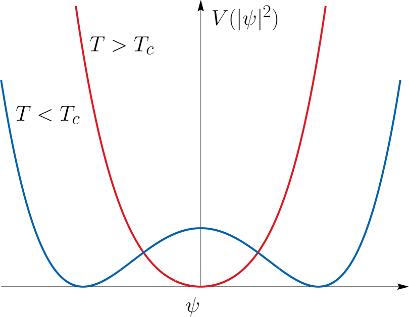
Figure A.1: The potential energy depending on the sign of the parameter $\alpha$. Above $T_{c}$, $\alpha>0$ and there is a unique minimum, while below $T_{c}$, $\alpha<0$ and the potential looks like the ‘mexican hat’.

In a first approximation, the parameter $\alpha$ is the only temperature dependent parameter

$$\alpha(T)=\alpha_{0}\left(\frac{T}{T_{c}}-1\right)\,.$$ (A.15)

This implies that above the critical temperature $T_{c}$, the parameter $\alpha>0$ and thus the normal state is energetically favoured. On the other hand, below the critical temperature $\alpha<0$, and the superconducting state is preferred. These two different regimes are qualitatively displayed in Fig. A.1.

Finally, the condensation energy, is defined as the energy difference between the normal state $\psi=0$ and the superconducting state $\psi_{0}$

$$f_{n}=\mathcal{F}(\psi=0)-\mathcal{F}(\psi_{0})=\frac{\alpha^{2}}{2\beta}=\frac{H_{c}^{2}}{2}$$ (A.16)

The value of magnetic field $H_{c}$ is called the thermodynamical critical magnetic field. While the external magnetic field penetrates without change, into the volume occupied by the normal state, it is expelled from the superconducting state. Thus, free energy of the normal state in a magnetic field $H>H_{ct}$ is lower than that of the uniform superconducting state, with expelled field. In the simplest case to be discussed below, $H_{ct}$ denotes the value of the external fields which destroys the superconductivity.

Length-scales in the Ginzburg-Landau theory

Borrowing the terminology of classical field theories, the length-scales are defined as the inverses masses of the mass spectrum of the theory. The mass spectrum of the theory is defined by the fluctuations of the fields around their ground state values. Since it is always possible to find a gauge where the ground state is $(\psi,{\bm{A}})_{\rm GS}=(\psi_{0},0)$, the perturbative expansion around the ground state, in terms of the infinitesimal parameter $\epsilon$ reads as

$$\psi=(\psi_{0}+\epsilon f)\exp\left\{i\epsilon\frac{\phi}{\psi_{0}}\right\}\,\leavevmode\nobreak\ \leavevmode\nobreak\ \leavevmode\nobreak\ \text{and}\leavevmode\nobreak\ \leavevmode\nobreak\ \leavevmode\nobreak\ {\bm{A}}=\epsilon{\bm{a}}\,.$$ (A.17)

Here, $f\equiv f(\mathbf{x})$ is the density amplitude, $\phi\equiv\phi(\mathbf{x})$ is the normalized phase amplitude, and ${\bm{a}}\equiv{\bm{a}}(\mathbf{x})$ are the gauge field fluctuations. The fluctuations are thus characterized by a system of Klein-Gordon equations for the two condensate fluctuations (one for the density plus one phase), and one Proca equation for the gauge field fluctuations. Choosing the gauge ${\bm{\nabla}}\!\cdot\!{\bm{a}}=0$, the system reads as

$$\frac{1}{2}\Upsilon^{T}\left(-{\bm{\nabla}}^{2}+{\cal M}^{2}\right)\Upsilon\,,\leavevmode\nobreak\ \leavevmode\nobreak\ \leavevmode\nobreak\ \text{where}\leavevmode\nobreak\ \leavevmode\nobreak\ \leavevmode\nobreak\ \Upsilon=(f,\phi,{\bm{a}})^{T}\,.$$ (A.18)

Here ${\cal M}^{2}$ is the squared mass matrix that is straightforwardly obtained by retaining the quadratic order of the infinitesimal parameter $\epsilon$, after introducing the expansion (A.17) into the free energy (A.2). The squared mass matrix can thus be read from

$$\Upsilon^{T}{\cal M}^{2}\Upsilon=2(\alpha+3\beta\psi_{0}^{2})f^{2}+e^{2}\psi_{0}^{2}{\bm{a}}^{2}\,.$$ (A.19)

Note that the fluctuation operator (A.18) and (A.19) can also be obtained by linearizing the equations of motion (A.4) and (A.5), in the expansion parameter $\epsilon$. The eigenspectrum of the matrix ${\cal M}^{2}$ determines the squared masses of the excitations and the corresponding normal modes. The inverse of each mass defines a characteristic length-scale of the theory. Overall, since the equations that define the mass spectrum of the fluctuations are

$${\bm{\nabla}}^{2}f=-4\alpha f\,,\leavevmode\nobreak\ \leavevmode\nobreak\ \leavevmode\nobreak\ \leavevmode\nobreak\ \leavevmode\nobreak\ \leavevmode\nobreak\ {\bm{\nabla}}^{2}\phi=0\,,\leavevmode\nobreak\ \leavevmode\nobreak\ \leavevmode\nobreak\ \text{and}\leavevmode\nobreak\ \leavevmode\nobreak\ \leavevmode\nobreak\ {\bm{\nabla}}^{2}{\bm{a}}=e^{2}\psi_{0}^{2}{\bm{a}}\,,$$ (A.20)

the masses are

$$m_{|\psi|}=2\sqrt{-\alpha}\,,\leavevmode\nobreak\ \leavevmode\nobreak\ \leavevmode\nobreak\ \leavevmode\nobreak\ \leavevmode\nobreak\ \leavevmode\nobreak\ m_{\varphi}=0\,,\leavevmode\nobreak\ \leavevmode\nobreak\ \leavevmode\nobreak\ \text{and}\leavevmode\nobreak\ \leavevmode\nobreak\ \leavevmode\nobreak\ m_{\bm{A}}=e\psi_{0}\,.$$ (A.21)

Here $m_{\varphi}=0$ is the Goldstone boson that gives mass to the longitudinal component of the gauge field [45]. Having obtained the mass spectrum (A.21), the relevant length-scales that characterize the superconducting ground state of the single-component Ginzburg-Landau model are

$$\xi=\frac{\sqrt{2}}{m_{|\psi|}}=\frac{1}{\sqrt{-2\alpha}}\,,\leavevmode\nobreak\ \leavevmode\nobreak\ \leavevmode\nobreak\ \leavevmode\nobreak\ \text{and}\leavevmode\nobreak\ \leavevmode\nobreak\ \leavevmode\nobreak\ \leavevmode\nobreak\ \lambda=\frac{1}{m_{\bm{A}}}=\frac{1}{e\psi_{0}}\,,$$ (A.22)

where $\xi$ is coherence length and $\lambda$ is the penetration depth. The factor $\sqrt{2}$ factor in the definition of coherence length is a matter of convention. This convention is that where the non-interacting regime (the Bogomol’nyi regime [153]), is $\kappa=1/\sqrt{2}$ for single-component superconductors [163].

The Ginzburg-Landau functional depends on three parameters, $\alpha$, $\beta$ and $e$. These determines the two fundamental length-scales: The coherence length $\xi$ of the superconducting condensate and the penetration depth $\lambda$ of the magnetic field. Actually the whole theory depends on a unique parameter $\kappa$, the Ginzburg-Landau parameter, defined as the ratio of the two length-scales:

$$\kappa=\frac{\lambda}{\xi}=\frac{\sqrt{2\beta}}{e}\,.$$ (A.23)

Alternative derivation of the mass spectrum:

The analysis above contains unphysical degrees of freedom. Indeed, as the gauge is not fixed there, the massless Goldstone mode appears. It is possible to find directly the physical mass spectrum of the theory, by rewriting the free energy (A.2), only in terms of the density and of the magnetic field. Given the definition of the supercurrent (A.5), the gradient term in the free energy can be written as

$$|{\bm{D}}\psi|^{2}=\left({\bm{\nabla}}|\psi|\right)^{2}+|\psi|^{2}({\bm{\nabla}}\varphi+e{\bm{A}})^{2}=\left({\bm{\nabla}}|\psi|\right)^{2}+\frac{{\bm{J}}^{2}}{e^{2}|\psi^{2}|}\,.$$ (A.24)

Hence, using the relation (A.24) together with the Ampère-Maxwell equation (A.5), the free energy (A.2) can be rewritten as

$$\mathcal{F} =\frac{1}{2}\left(\frac{{\bm{J}}^{2}}{e^{2}|\psi^{2}|}+{\bm{B}}^{2}\right)+\frac{1}{2}\left({\bm{\nabla}}|\psi|\right)^{2}+\alpha|\psi|^{2}+\frac{\beta}{2}|\psi|^{4}$$ (A.25a)

$$=\frac{1}{2}\left(\frac{({\bm{\nabla}}\!\times\!{\bm{B}})^{2}}{e^{2}|\psi^{2}|}+{\bm{B}}^{2}\right)+\frac{1}{2}\left({\bm{\nabla}}|\psi|\right)^{2}+\alpha|\psi|^{2}+\frac{\beta}{2}|\psi|^{4}\,.$$ (A.25b)

Expressing the free energy in such a way has the advantage to stress the dependence on the gauge invariant physical degrees of freedom explicitly. Returning to the investigation of the mass spectrum, the perturbative expansion around the ground state, in terms of the infinitesinal parameter $\epsilon$ reads as

$$|\psi|=\psi_{0}+\epsilon f\,\leavevmode\nobreak\ \leavevmode\nobreak\ \leavevmode\nobreak\ \text{and}\leavevmode\nobreak\ \leavevmode\nobreak\ \leavevmode\nobreak\ {\bm{B}}=\epsilon e\psi_{0}{\bm{b}}\,.$$ (A.26)

Here, $f\equiv f(\mathbf{x})$ is the density amplitude, ${\bm{b}}\equiv{\bm{b}}(\mathbf{x})$ are the magnetic field fluctuations. In contrast with the expansion (A.17), the expansion (A.26) depends only on the physical fields. The fluctuations are thus characterized by a system of one Klein-Gordon equation for the condensate fluctuations, and one Proca equation for the magnetic field fluctuations. Introducing the expansion (A.26) into the free energy (A.2), and retaining the quadratic order of the infinitesimal parameter $\epsilon$ yields the equation

$$\frac{1}{2}\Upsilon^{T}\left(-{\bm{\nabla}}^{2}+{\cal M}^{2}\right)\Upsilon\,,\leavevmode\nobreak\ \leavevmode\nobreak\ \leavevmode\nobreak\ \text{where}\leavevmode\nobreak\ \leavevmode\nobreak\ \leavevmode\nobreak\ \Upsilon=(f,{\bm{b}})^{T}\,.$$ (A.27)

The squared mass matrix ${\cal M}^{2}$ can be read from

$$\Upsilon^{T}{\cal M}^{2}\Upsilon=2(\alpha+3\beta\psi_{0}^{2})f^{2}+e^{2}\psi_{0}^{2}{\bm{b}}^{2}\,.$$ (A.28)

Again, the eigenspectrum of the matrix ${\cal M}^{2}$ determines the squared masses of the excitations

$$m_{|\psi|}=2\sqrt{-\alpha}\,,\leavevmode\nobreak\ \leavevmode\nobreak\ \leavevmode\nobreak\ \text{and}\leavevmode\nobreak\ \leavevmode\nobreak\ \leavevmode\nobreak\ m_{\bm{B}}=e\psi_{0}\,,$$ (A.29)

and the associated length-scales $\xi$ and $\lambda$ are obviously the same as in (A.22).

Meissner effect

The Meissner effect is the expulsion of a magnetic field from a superconductor, when it is in the superconducting state. In a weak external applied field, the superconductor expels (almost) all magnetic flux, by setting up surface currents. This relates to the above mentioned fact, that the Ampère-Maxwell equation becomes a Proca equation on a constant superconducting ground state $|\psi|=\psi_{0}=\sqrt{\frac{-\alpha}{\beta}}$. This is more intuitive physically, when considering the London equation for the magnetic field. On a constant superconducting state $\psi=\psi_{0}$, taking the curl of the Ampère’s equation (A.5), yields the London equation

$${\bm{\nabla}}\!\times\!{\bm{\nabla}}\!\times\!{\bm{B}}+e^{2}\psi_{0}^{2}{\bm{B}}=0\leavevmode\nobreak\ \leavevmode\nobreak\ \leavevmode\nobreak\ \leavevmode\nobreak\ \Leftrightarrow\leavevmode\nobreak\ \leavevmode\nobreak\ \leavevmode\nobreak\ \leavevmode\nobreak\ {\bm{\nabla}}^{2}{\bm{B}}=e^{2}\psi_{0}^{2}{\bm{B}}\leavevmode\nobreak\ \leavevmode\nobreak\ \leavevmode\nobreak\ \leavevmode\nobreak\ \leavevmode\nobreak\ \leavevmode\nobreak\ (\text{since}\leavevmode\nobreak\ {\bm{\nabla}}\!\times\!{\bm{\nabla}}\!\times\!{\bm{B}}={\bm{\nabla}}({\bm{\nabla}}\!\cdot\!{\bm{B}})-{\bm{\nabla}}^{2}{\bm{B}})\,.$$ (A.30)

The London equation thus turns into a Helmholtz equation for the magnetic field, with the eigenvalue of the Laplacian $m_{\bm{B}}=e\psi_{0}$. In other words, the magnetic field is a massive vector field of squared mass $m_{\bm{B}}^{2}=e^{2}|\psi_{0}|^{2}$. This defines a length-scale, as the inverse mass of the magnetic field, called the London penetration depth $\lambda=1/m_{\bm{B}}=1/e|\psi_{0}|$. The London equation (A.30) implies that an externally applied field decays exponentially inside the superconductor with the decay length given by $\lambda$. Alternatively, as demonstrated earlier, the London penetration depth can be understood as the length-scale, at which a small fluctuation of the vector potential recovers to its ground state value ${\bm{A}}=0$.

A.2 Interface energy – Type-I/type-II dichotomy

Now, consider the full non-linear problem of the interface between the normal state and the superconducting state, in an external field ${\bm{H}}_{e}=(0,0,H)$. The value of the external magnetic field is set equal to the thermodynamical critical field $H_{c}$. The associated magnetic field reads as ${\bm{B}}=(0,0,B(x))$. The interface is located at $x=0$ and the normal state fills the semi-infinite space $x<0$, while $x>0$ corresponds to the bulk superconductor. As the problem is considered in an external field, the relevant energy is the Gibbs energy (A.3).

On the right boundary, far in the bulk superconductor, the superconducting state completely recovers. On the left boundary, this is the normal state in an external field $H_{c}$. This sets the boundary conditions

$$\psi(x\to+\infty) =\psi_{0}\leavevmode\nobreak\ \leavevmode\nobreak\ \leavevmode\nobreak\ \leavevmode\nobreak\ \text{and}\leavevmode\nobreak\ \leavevmode\nobreak\ \leavevmode\nobreak\ \leavevmode\nobreak\ {\bm{B}}(x\to+\infty)=0\,,$$ (A.31a)

$$\psi(x\to-\infty) =0\leavevmode\nobreak\ \leavevmode\nobreak\ \leavevmode\nobreak\ \leavevmode\nobreak\ \leavevmode\nobreak\ \leavevmode\nobreak\ \text{and}\leavevmode\nobreak\ \leavevmode\nobreak\ \leavevmode\nobreak\ \leavevmode\nobreak\ {\bm{B}}(x\to-\infty)=H_{c}\,.$$ (A.31b)

As a result, the values of the Gibbs energy on these boundaries are $\mathcal{G}(x\to+\infty)=\mathcal{F}(|\psi_{0}|)$ (the free energy of a superconductor without an external field) and $\mathcal{G}(x\to-\infty)=f_{n}-H_{c}^{2}/2$ (since the free energy of the normal state in external field is $\mathcal{F}=f_{n}+H_{c}^{2}/2$). The interface energy (or boundary surface energy between normal and superconducting state) is defined as the difference

$$\sigma_{ns} =\int_{-\infty}^{+\infty}\Big{(}\mathcal{G}(x)-f_{n}+\frac{H_{c}^{2}}{2}\Big{)}dx$$ (A.32a)

$$=\int_{-\infty}^{+\infty}\Big{(}\frac{|{\bm{B}}-H_{c}|^{2}}{2}+\frac{1}{2}|{\bm{D}}\psi|^{2}+\alpha|\psi|^{2}+\frac{\beta}{2}|\psi|^{4}\Big{)}dx$$ (A.32b)

The evaluation of the interface energy (A.32) has to be done numerically. However, in the limiting cases $\kappa\gg 1$ and $\kappa\ll 1$, it can be estimated analytically.

In the $\kappa\gg 1$, $|\psi|$ recovers its ground state value $\psi_{0}$ very quickly. Thus, the energy cost associated with the density gradients can be neglected. Now the problem reduces to dealing with the screening of the magnetic field in a region of width $\lambda$. The associated interface energy is

$$\sigma_{ns}(\kappa\gg 1)=\int_{-\infty}^{+\infty}\Big{(}\frac{\lambda^{2}}{2}B^{\prime 2}+\frac{1}{2}B^{2}-BH_{c}\Big{)}dx\,,$$ (A.33)

where ^′ denotes the differentiation with respect to $x$ and $B=B_{0}\mathrm{e}^{-x/\lambda}$. This give a negative interface energy

$$\sigma_{ns}(\kappa\gg 1)\approx\frac{H_{c}^{2}\lambda}{2}=-\frac{1}{2e}\frac{(-\alpha)^{3/2}}{\beta^{1/2}}\,.$$ (A.34)

In the limit where $\kappa\ll 1$ the magnetic field is much more localized than the superconducting condensate. It is screened at the length-scale $\lambda$, which is much smaller than the coherence length $\xi$. This means that the dominant contribution to the energy comes from the condensate $\psi$. As a result the boundary of width $\xi$ is approximated by

$$\sigma_{ns}(\kappa\ll 1) =\frac{\alpha^{2}}{2\beta}\int_{-\infty}^{+\infty}\Big{(}4\xi^{2}|\tilde{\psi}|^{\prime 2}+(1-|\tilde{\psi}|^{2})^{2}\Big{)}dx\,,$$ (A.35)

where $\tilde{\psi}=\psi/\psi_{0}$. Substituing, $\tilde{\psi}=\tanh(x/2\xi)$, estimates the integral

$$\sigma_{ns}(\kappa\ll 1)\approx\frac{4\alpha^{2}}{3\beta}\xi=\frac{(-2\alpha)^{3/2}}{3\beta}\,,$$ (A.36)

which is positive.

In the limit where $\kappa\gg 1$, the interface energy (A.34) is negative, while it is positive in the limit $\kappa\ll 1$ (A.36). The crossover between positive and negative interface energies is obtained for the critical value $\kappa=1/\sqrt{2}$. The sign of the interface energy determines the division between two classes of superconductors. The type-1 superconductors ($\kappa<1/\sqrt{2}$) have a positive interface energy ($\sigma_{ns}>0$), while the type-2 superconductors ($\kappa>1/\sqrt{2}$) have a negative interface energy ($\sigma_{ns}<0$).

Physically this means that in type-1 superconductors there is an energy penalty for forming interfaces. This results in a preference for forming macroscopically large normal domains that minimize the length of the interface. In type-2 superconductors, this is the opposite. Since the interface energy is negative, it is beneficial to have the maximal length of interface. And thus creating large number of small domains. These small domains are the vortices which are discussed in the next section.

A.3 Quantization of the magnetic flux – Vortices

The Stokes’ theorem implies that the flux of the magnetic field through a given area ${\cal A}$ can be expressed as the line integral over the contour ${\cal C}$ bounding that area $\Phi=\int_{\cal A}{\bm{B}}\!\cdot\!d{\bm{S}}=\oint_{\cal C}{\bm{A}}\!\cdot\!d{\bm{\ell}}$. Given the definition of the current (A.5), the vector potential ${\bm{A}}$ can be written in terms of the phase gradient ${\bm{\nabla}}\varphi$ and the current ${\bm{J}}$. It follows that the magnetic flux reads as

$$\Phi=\frac{1}{e}\bigointsss_{\!\!\!\!\!\!{\cal C}}\left(\frac{{\bm{J}}}{e^{2}|\psi|^{2}}-{\bm{\nabla}}\varphi_{a}\right)\!\cdot\!d{\bm{\ell}}\,.$$ (A.37)

Since in the bulk of the superconductor, $|\psi|$ quickly converges to its ground state $\psi_{0}$ and that ${\bm{J}}$ decays exponentially fast due to Meissner screening, the magnetic flux through ${\cal A}$ reads as

$$\Phi=\frac{-1}{e}\bigointsss_{\!\!\!\!\!\!{\cal C}}{\bm{\nabla}}\varphi\cdot{d\bm{\ell}}\,.$$ (A.38)

Since $\psi$ has to be single-valued, the circulation of phase can only take values $2\pi n$ where $n$ is an integer. As a result, the associated flux is

$$\Phi=\frac{-2\pi}{e}n=\Phi_{0}n\,.$$ (A.39)

The flux is thus quantized in units of $\Phi_{0}=-2\pi/e$, the flux quantum. The integer $n$, called the winding number, counts the number of times the phase $\varphi$ winds along the (large) contour ${\cal C}$. The winding number, which is defined as a line integral over a closed path, is related to the maps $\mathbb{S}^{1}\to\mathbb{S}^{1}$. It is associated with the elements of the first homotopy of the circle: $n\in\pi_{1}(\mathbb{S}^{1})=\mathbb{Z}$.

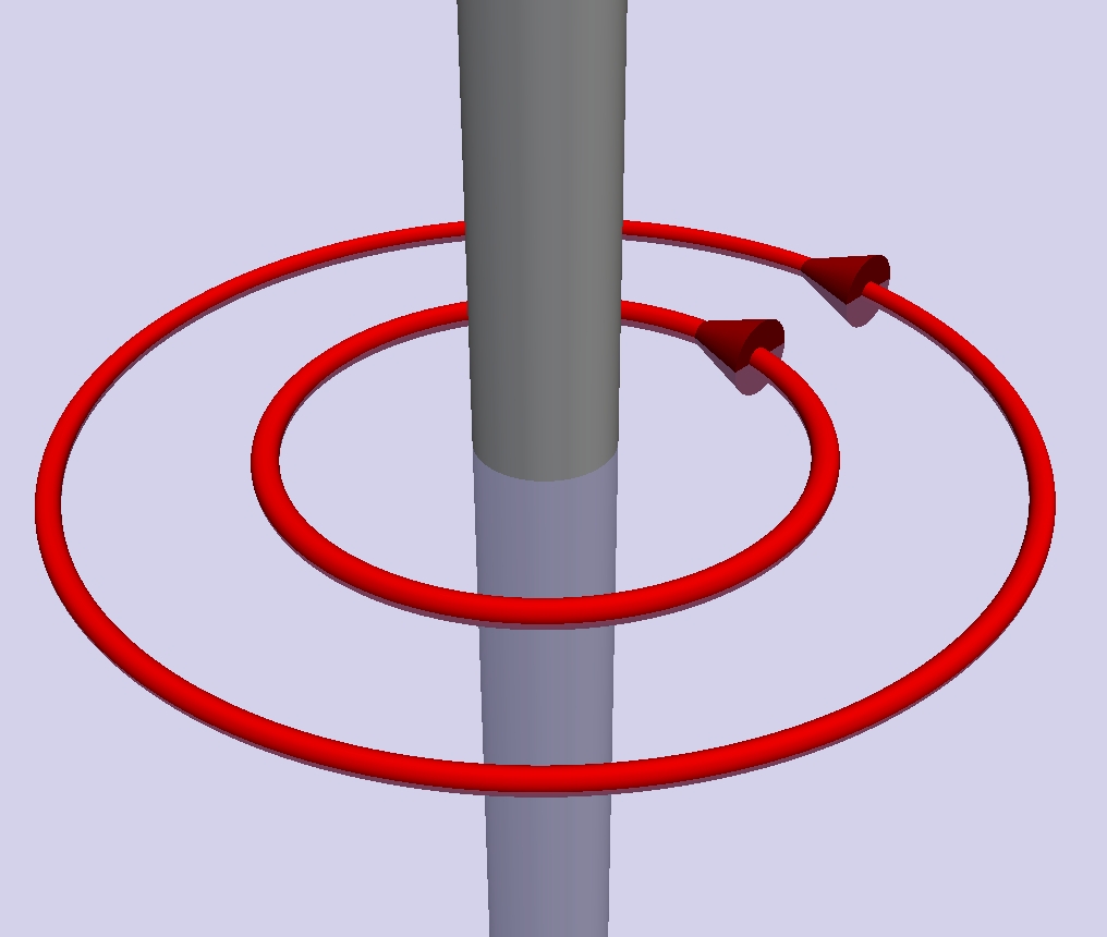
Figure A.2: Schematic illustration of a singular vortex line surrounded by screening currents.

If a configuration have a non-zero phase winding, then the density ($|\psi|$) should vanish at the point around which the phase winds. The phase winding is compensated by having a non-trivial configuration of ${\bm{A}}$ that carries quantized flux. Thus, the magnetic field cannot penetrate into the bulk of a superconductor without causing a singular vortex.

The finiteness of the energy imposes that at spatial infinity, the condensate has to be of constant modulus $\psi_{0}$ with an integer phase winding, and ${\bm{A}}$ has to be a pure gauge. Assuming axial symmetry, in cylindrical coordinates, the fields can be parametrized as

$$\psi=f(\rho)\mathrm{e}^{in\theta}\,,\leavevmode\nobreak\ \leavevmode\nobreak\ \leavevmode\nobreak\ \text{and}\leavevmode\nobreak\ \leavevmode\nobreak\ \leavevmode\nobreak\ {\bm{A}}=v(\rho)(\sin\theta,-\cos\theta)\,.$$ (A.40)

This is the Abrikosov-Nielsen-Olesen ansatz [151, 30] which simplifies the Ginzburg-Landau equation (A.4) and (A.5) to a set of two ordinary differential equations. Yet these equations are nonlinear, so they cannot, in general, be solved analytically. A typical vortex configuration is sketched on the figure A.2. A vortex is a singular line around which circulate Meissner currents, that screen the magnetic field away from the vortex. Typical vortex profiles in the type-1 and type-2 regimes are displayed in Fig. A.3.

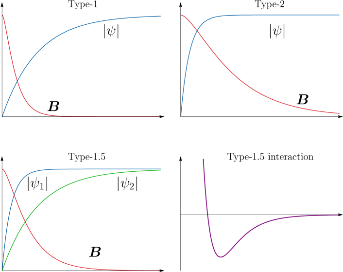
Figure A.3: The panels illustrate the vortex profiles in single-component type-1 and type-2 regimes.

Vortex interaction: Type-I/type-II dichotomy

As previously emphasized, depending on the value of the Ginzburg-Landau parameter $\kappa$, superconductors can classified into two different classes; type-1 and type-2. This classification followed from the different behaviour of interface energy between the normal and superconducting state. This dichotomy can also be understood by considering the interaction between vortices that should form in an external field.

In the case of type-2 superconductors, i.e. for $\kappa>1/\sqrt{2}$, the long-range interaction between vortices is dominated by the the magnetic interaction. It follows that vortices repel (as is also the case in the London limit $\kappa\gg 1$). On the other hand, for type-1 superconductors, i.e. for $\kappa<1/\sqrt{2}$, the attractive interaction between the cores dominates the magnetic interactions at all separations. As a result, in the regime where $\xi>/\sqrt{2}\lambda$, separated vortices will collapse onto each other to form a vortex with a larger winding number (a megavortex). This leads to the formation of the macroscopically large domains of the normal state. Note that this is obviously consistent with the results from the interface energy where, when $\kappa<1/\sqrt{2}$ it is beneficial to minimize the interface area. In the limiting case where $\kappa=1/\sqrt{2}$, i.e. when $\xi=\sqrt{2}\lambda$, the vortices are non-interacting [152, 153]. More precisely, the repulsion due to the magnetic field exactly compensates the attraction of the cores. This non-interacting regime is called the Bogomol’nyi point of the phase diagram.

The properties of the vortex matter and their interactions, in the single-component Ginzburg-Landau for conventional superconductors, can thus be summarized as follows

• Type-1 : $\sqrt{2}\lambda<\xi$: The vortices attract each other to form macroscopically large domains.

• BP : $\sqrt{2}\lambda=\xi$: the vortices are non-interacting and all vortex superpositions have the same energy [152, 153].

• Type-2 : $\sqrt{2}\lambda>\xi$: The vortices repel each other to form a vortex lattice [151].

The qualitative difference between the type-1 and type-2 regimes can be seen in the vortex profiles displayed in the Fig. A.3.

A.4 Phase diagrams and critical fields

As stated earlier, in the presence of an applied external field ${\bm{H}}_{e}$, this is the Gibbs free energy (A.3) that should be considered instead of the Helmholtz free energy $F$ (A.2). The response to an applied external magnetic field is summarized in the diagrams Fig. A.4.

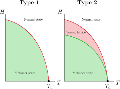
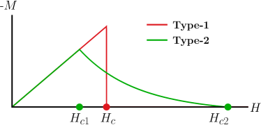
Figure A.4: Phase diagrams of the different regimes in single-component Ginzburg-Landau theory. The two $H-T$ diagrams sketch the difference between the response of type-1 and type-2 superconductors to an external field $H$. As discussed below, in the type-2 regime, since the first critical field is smaller that the thermodynamical critical field, there exist an intermediate state between the Meissner state and the normal state. This intermediate state is that of a vortex lattice. The rightmost panel shows the difference of the magnetization response $M$ between type-1 and type-2. The type-1 regime features a first order phase transition between the superconducting state and the normal state. In the type-2 regime, at the level of mean-field theory, there are second order phase transitions between Meissner and vortex states and between vortex and normal states.

First critical field

The first critical field $H_{c1}$ is defined as the applied magnetic field at which the formation of a single vortex becomes energetically favourable. In other words, $H_{c1}$ is the thermodynamic field at which the presence of vortices into the sample becomes energetically favourable as compared to the Meissner state. It is defined as $H_{c1}=E_{v}/\Phi_{v}$, where $E_{v}$ and $\Phi_{v}$ are the energy and magnetic flux of the vortex. That is

$$H_{c1}=\frac{\int(\mathcal{F}(\psi_{v},{\bm{A}}_{v})-\mathcal{F}(\psi_{0},0))}{\int{\bm{\nabla}}\!\times\!{\bm{A}}}\,,$$ (A.41)

where $(\psi_{0},0)$ denotes the ground state configuration of the superconducting condensates and $(\psi_{v},{\bm{A}}_{v})$, the configuration of a vortex. Note however that the corresponding external field ${\bm{H}}_{e}$ should be smaller than the thermodynamical critical magnetic field $H_{ct}$ (A.16)

$$H_{ct}=2\sqrt{\mathcal{F}(0,0)-\mathcal{F}(\psi_{0},0)}\,,$$ (A.42)

above which it is no longer beneficial to form a superconducting condensate.

If the first critical field is smaller than the thermodynamical critical field $H_{c1}<H_{ct}$ (this is the case for type-2 and not for type-1), then vortices start to enter the superconductor. Thus in the type-2 regime, increasing the applied field, results in an intermediate state between the Meissner and normal states.

Second critical field

When higher field is applied, more and more vortices enter the system. They repel each other with length-scale given by $\lambda$. When vortices are more and more packed, and vortex cores start to overlap. This results in an overall suppression of the density $|\psi|$, so that there is a certain value of the field that completely destroys the superconductivity. This value of the field is called the second critical field at which superconductivity is destroyed. Thus, close to the second critical field $H_{c2}$, the magnetic field is approximately constant, ${\bm{B}}=B\bm{e}_{z}=H\bm{e}_{z}$ and the density $|\psi|$ is small. As a result, the Ginzburg-Landau equation can be linearized

$${\bm{D}}{\bm{D}}\psi=2\alpha\psi\,.$$ (A.43)

In the Landau gauge, the vector potential reads as ${\bm{A}}=(0,Hx,0)^{-1}$. There, the equation (A.43) do not depend on $y$, so a convenient choice (in a first approximation) of variable separation is $\psi\equiv\psi(x)$. The linearized Ginzburg-Landau equation (A.43) thus becomes the equation of an harmonic oscillator:

$$\psi^{\prime\prime}-(eHx)^{2}\psi=2\alpha\Psi\,.$$ (A.44)

Thus the solution has the form $\psi(x)=C\exp\left(-\frac{x^{2}}{2\ell^{2}}\right)$ with the arbitrary constant $C$ and $eH=1/\ell^{2}$. The equation (A.44) further simplifies

$$eH_{c2}=\frac{1}{\ell^{2}}\equiv-2\alpha=\frac{1}{\xi^{2}}\,.$$ (A.45)

As a result,

$$H_{c2}=\frac{1}{e\xi^{2}}=\frac{\Phi_{0}}{2\pi\xi^{2}}\,.$$ (A.46)

Note that this means in particular that close to $H_{c2}$, there is one (diverging) length-scale.

The thermodynamical critical field (A.16) is $H_{c}^{2}=\alpha^{2}/\beta=e^{-2}\xi^{-2}\lambda^{-2}/2$. Hence the ratio of the second critical field with the thermodynamical critical field is

$$\frac{H_{c2}}{\sqrt{2}H_{c}}=\frac{\lambda}{\xi}=\kappa\,.$$ (A.47)

In terms of the critical fields, type-1 and type-2 superconductors have the phase diagram summarized in Fig. A.4. Type-1 and type-2 superconductors, thus have a different behaviour in an external field, summarized in the phase diagrams in Fig. A.4. For type-1, the critical field simply destroys superconductivity to favour the normal state. In type-2 superconductors, when the applied field ${\bm{H}}_{e}$ exceeds $H_{c1}$ the magnetic field starts to penetrate the bulk superconductor in the form of quantized vortices.

Appendix B Numerical methods

Many of the results discussed in the main body rely on numerical simulations, but the focus is made on the physical properties and very few words are said about these simulations. Here is a detailed discussion of the numerical methods used to investigate the physics discussed in the main part. This starts, in Section B.1, with a general overview of the finite element methods used for the spatial discretization. Next, details of the algorithm used to solve the (nonlinear) Ginzburg-Landau problems are discussed in the Section B.2. The important aspects of having a suitable choice of an initial guess, are detailed in the Section B.2.3. Finally, the question of the evolution of time-dependent problems is addressed in the Section B.3.

B.1 Basic concepts for Finite Element methods

There exists various approaches to address the spatial discretization of partial differential equations. The finite difference method, which is based upon local Taylor expansions to approximate the derivative, is most historical. This discretization technique covers the space with lattices which are topologically square or cuboid network. This method is rather intuitive, but it makes it difficult to handle complex geometries. This difficulty motivated the approach of the finite element method. The finite element methods have often been historically preferred for their rigorous provable stability, and because of their natural applicability to complex geometries. The relative advantages of both methods have been heavily debated, and it is fair to say that nowadays both methods lie more or less on the same ground. Both with their own advantages and difficulties. There exist many more different approaches, such as the spectral methods, which will not be exhaustively listed here. Finite differences or finite elements methods are more or less frequent, depending on the different scientific communities. For example, and very roughly speaking, finite differences are extensively used for simulations of lattice gauge theories, while finite elements are customary for example in engineering and mathematics.

The numerical investigations discussed in the main body, and the corresponding papers, extensively used finite element methods for a broad variety of problems including direct solving, minimization, constrained optimization, time-evolution, etc. In practice, the spatial discretization is handled within a the finite-element framework provided by the FreeFEM++ library [317]. There, the finite element methods are based one the weak formulation (the variational formulation) of partial differential equation. Below is presented a brief and non exhaustive description of the concepts used in finite element methods. Detailed introductions can be found in many textbooks, see for example [318, 319, 320, 321].

B.1.1 Finite-element formulation

Consider the domain $\Omega$ which a bounded open subset of $\mathbbm{R}^{d}$ and denote $\partial\Omega$ its boundary. $W^{k,p}(\Omega)$ denotes the Sobolev space of order $k$ on $\Omega$. That is, the subset of functions $f$ in $L^{p}(\Omega)$ such that $f$ and their weak derivatives have a finite $L^{p}$-norm up to order $k$. The Hilbert space equipped with the $L^{2}$-norm is denoted $H^{k}(\Omega)=W^{k,2}(\Omega)$, and $\mathcal{H}^{k}_{\Omega}=\{u+iv\,|\,u,v\in H^{k}(\Omega)\}$ denotes the Hilbert spaces of complex-valued functions. The inner products are denoted by $\langle\cdot,\cdot\rangle$, as for example:

$$\left\langle u,v\right\rangle=\int_{\Omega}uv\,,\leavevmode\nobreak\ \text{for}\leavevmode\nobreak\ u,v\in H^{k}({\Omega})\,,\leavevmode\nobreak\ \leavevmode\nobreak\ \leavevmode\nobreak\ \leavevmode\nobreak\ \text{and}\leavevmode\nobreak\ \leavevmode\nobreak\ \leavevmode\nobreak\ \leavevmode\nobreak\ \left\langle u,v\right\rangle=\int_{\Omega}u^{*}v\,,\leavevmode\nobreak\ \text{for}\leavevmode\nobreak\ u,v\in\mathcal{H}^{k}({\Omega})\,.$$ (B.1)

Once the equations are formulated in their weak form, the appropriate Hilbert spaces have to be discretized using finite element spaces for a given partition $\mathcal{T}_{h}$ of $\Omega$.

Figure B.1: Example of the mesh of a disc.

More precisely, $\mathcal{T}_{h}$ is a regular partition of the domain $\Omega$ with $\Omega=\cup_{k=1}^{n_{t}}\Omega_{k}$. The name $\mathcal{T}_{h}$ refers to the family $\{T_{k}\}_{k=1,\cdots,n_{t}}$ of the $n_{t}$ triangles that compose the mesh, as illustrated for example in Fig. B.1. Typically $h$ refers to the mesh size $h=\mathrm{max}_{\Omega_{k}\in\mathcal{T}_{h}}\{\mathrm{diam}\,\Omega_{k}\}$. In practice, for a given boundary of the domain, the mesh can be automatically generated using for example the Delaunay-Voronoi algorithm. Next, given a spatial discretization, the functions are approximated to belong to a finite element space whose properties correspond to the details of the Hilbert space to which the functions belong. A finite element space associated to a scalar function, say $w$, is typically, a space of polynomial functions $\mathrm{P}^{(r)}$ of order $r$ on the elements (the triangles), with certain matching properties at edges, vertices, etc. $\mathrm{P}^{(r)}$ denotes the $r$-th order Lagrange finite-elements. This describes a linear vector space of finite dimension, for which a basis can be found. The canonical basis is made of functions, called the hat functions $\phi_{k}$ and thus

$$V_{h}(\mathcal{T}_{h},\mathrm{P}^{(r)})=\Big{\{}w(\mathbf{x})=\sum_{k=1}^{M}w_{k}\phi_{k}(\mathbf{x}),\phi_{k}(\mathbf{x})\in\mathrm{P}^{(r)}\Big{\}}\,.$$ (B.2)

Here $M$ is the dimension of $V_{h}$ (the number of vertices), the $w_{k}$ are called the degree of freedom of $w$ and $M$ the number of the degrees of freedom. Now for a given order of approximation of polynomial functions $\mathrm{P}^{(r)}$, the shape functions $\phi_{k}(\mathbf{x})$ are constructed from the triangle $T_{k}$. For example $V_{h}(\mathcal{T}_{h},\mathrm{P}^{(1)})$ denotes the space of continuous, piecewise linear functions of $x$, $y$ on each triangle of $\mathcal{T}_{h}$. To summarize a given function is approximated as its decomposition:

$$w(\mathbf{x})=\sum_{k=1}^{M}w_{k}\phi_{k}(\mathbf{x})\,,$$ (B.3)

on a given basis of $\phi_{k}(\mathbf{x})$ that is chosen according to the mathematical prescriptions of the problem.

B.1.2 A simple example: The Poisson equation

To illustrate the concept of weak formulation of partial differential equations, let consider the simple case of the Poisson equation with Dirichlet condition $u=0$ on $\partial\Omega$:

$$\nabla^{2}u=f\,.$$ (B.4)

The weak form, or variational form, is derived by multiplying (B.4) by an arbitrary test function $v$ and integrating over $\Omega$:

$$-\int_{\Omega}v\nabla^{2}u+\int_{\Omega}vf= 0$$ (B.5a)

$$\int_{\Omega}{\bm{\nabla}}u\cdot{\bm{\nabla}}v+\int_{\Omega}vf= \int_{\partial\Omega}v{\bm{\nabla}}u\cdot{\bf n}\,,$$ (B.5b)

where the second line follows from the Green’s formula (integration by parts), and ${\bf n}$ is the outgoing vector normal to $\partial\Omega$. The test functions $v$ should satisfy the boundary condition $v=0$ on $\partial\Omega$, and thus the problem can be written as

$$a(u,v)+\ell(f,v)=0$$ (B.6)

with $a(u,v)=\left\langle{\bm{\nabla}}u,{\bm{\nabla}}v\right\rangle$ and $\ell(f,v)=\left\langle f,v\right\rangle$. The weak form (B.6) defines a linear algebraic system. Indeed inserting a finite element decomposition, as in (B.3), into (B.6), the problem boils down to

$$\sum_{k=1}^{M}A_{ik}u_{k}+L_{i}=0\,,\text{with}\leavevmode\nobreak\ \leavevmode\nobreak\ L_{i}=\left\langle f,\phi_{i}(\mathbf{x})\right\rangle\,,$$ (B.7)

for all $i=0,\cdots,M-1$. $L_{i}$ is a vector and $A_{ik}$ is called the stiffness matrix. In a matrix notation, the Poisson equation problem (B.4) reads as

$$\left[{\bm{A}}\right]\left[u_{h}\right]+\left[{\bm{L}}\right]=0\,,$$ (B.8)

whose solution simply requires the inversion of the stiffness matrix $\left[{\bm{A}}\right]$:

$$\left[u_{h}\right]=-\left[{\bm{A}}\right]^{-1}\left[{\bm{L}}\right]\,.$$ (B.9)

Note that the stiffness matrix $\left[{\bm{A}}\right]$ is a sparse matrix, which can in principle be efficiently preconditioned. Variety of numerical tools and libraries are available to perform linear algebra operations such as the matrix inversion.

B.1.3 A less simple example: The Ampère-Maxwell equation

As a further example, let’s consider the Ampère-Maxwell equation with the boundary condition ${\bm{B}}={\bm{B}}_{0}$ on $\partial\Omega$:

$${\bm{\nabla}}\!\times\!{\bm{B}}+{\bm{J}}=0\,.$$ (B.10)

Again, the weak form is derived by multiplying (B.10) by an arbitrary test function ${\bm{A}}^{v}$ and integrating over $\Omega$:

$$\int_{\Omega}{\bm{\nabla}}\!\times\!{\bm{A}}^{v}\cdot{\bm{B}}+\int_{\partial\Omega}{\bm{A}}^{v}\times{\bf n}\cdot{\bm{B}}+\int_{\Omega}{\bm{A}}^{v}\cdot{\bm{J}}= 0$$ (B.11a)

$$\int_{\Omega}{\bm{\nabla}}\!\times\!{\bm{A}}^{v}\cdot{\bm{\nabla}}\!\times\!{\bm{A}}+\int_{\Omega}{\bm{A}}^{v}\cdot{\bm{J}}= \int_{\partial\Omega}{\bf n}\times{\bm{A}}^{v}\cdot{\bm{B}}_{0}\,,$$ (B.11b)

where the magnetic field on the r.h.s. of (B.11b) has been replaced by the boundary condition ${\bm{B}}={\bm{B}}_{0}$ (${\bf n}$ is the outgoing vector normal to $\partial\Omega$). The problem can be written as

$$a({\bm{A}},{\bm{A}}^{v})+\ell({\bm{J}},{\bm{A}}^{v})=0$$ (B.12)

with $a({\bm{A}},{\bm{A}}^{v})=\left\langle{\bm{\nabla}}\!\times\!{\bm{A}},{\bm{\nabla}}\!\times\!{\bm{A}}^{v}\right\rangle$ and $\ell({\bm{J}},{\bm{A}}^{v})=\left\langle{\bm{J}},{\bm{A}}^{v}\right\rangle$. Here, the scalar product acts on the vectorial space. For detailed discussions, see e.g. [322, 323]. Again, inserting the finite element decomposition for ${\bm{A}}$ defines a linear system that can be solved similarly to the discussion in Sec. B.1.2. Note that in the case of Ginzburg-Landau models, the current ${\bm{J}}$ depends on the gauge field ${\bm{A}}$.

B.2 Minimization of the Ginzburg-Landau free energy

Many of the problems discussed in the main body require to numerically minimized the Ginzburg-Landau free energy. This is a non-trivial nonlinear optimization problem for a field theory. The choice of the discretization of the fields was usually done within the finite element formulation discussed in the previous section, an the choice for the optimization algorithm was typically the Non-Linear Conjugate Gradient method. Below, are briefly introduced the principles of this method, while the actual formulation of the Ginzburg-Landau minimization problem is discussed after.

B.2.1 The Nonlinear Conjuguate Gradient method

The NonLinear Conjugate Gradient method (NLCG) is a numerical method to solve iteratively unconstrained optimization problems. It is used to find a local minimum of a nonlinear function $f(\mathbf{x})$ using only its gradient $\nabla_{\mathbf{x}}f$ (unlike the Newton-Raphson method that needs the second variation of the function). This method requires the function $f$ to be approximately quadratic close to the minimum. That is, the function should be twice differentiable and the second derivative should be non-singular, near the minimum [324, 325, 326, 327]. Given the function of $n$ variables, the conjugate gradient method aims at solving the nonlinear, unconstrained optimization problem

$$\min\{f(\mathbf{x})|\mathbf{x}\in\mathbbm{R}^{n}\}\,,$$

where $f:\mathbbm{R}^{n}\mapsto\mathbbm{R}$ is continuously differentiable and bounded from below. Starting from an initial guess $\mathbf{x}_{0}\in\mathbbm{R}^{n}$, the nonlinear conjugate gradient method generates a recurrence

$$\mathbf{x}_{k+1}=\mathbf{x}_{k}+\alpha_{k}{\bm{d}}_{k}\,.$$

Here, $\alpha_{k}$ is a (positive) step size obtained by a line search. The conjugate direction ${\bm{d}}_{k}$ is generated by the rule

$${\bm{d}}_{k}=-{\bm{g}}_{k}+\beta_{k-1}{\bm{d}}_{k-1}\,.$$

Here ${\bm{g}}_{k}$ is a column vector of the gradient of $f$ in all directions, ${\bm{g}}_{k}=\nabla_{\mathbf{x}}f(\mathbf{x}_{k})$. Finally $\beta_{k}$ is the conjugate gradient parameter that can be updated according to different rules [326]. The most common update rules are those of Fletcher-Reeves [328] and Polak-Ribière-Polyak [329, 330]; these are defined as:

$$\beta_{k-1}^{FR}=\frac{{\bm{g}}^{T}_{k}{\bm{g}}_{k}}{{\bm{g}}^{T}_{k-1}{\bm{g}}_{k-1}}\,,\leavevmode\nobreak\ \leavevmode\nobreak\ \leavevmode\nobreak\ \text{and}\leavevmode\nobreak\ \leavevmode\nobreak\ \leavevmode\nobreak\ \beta_{k-1}^{PRP}=\frac{{\bm{g}}^{T}_{k}({\bm{g}}_{k}-{\bm{g}}_{k-1})}{{\bm{g}}^{T}_{k-1}{\bm{g}}_{k-1}}\,.$$ (B.13)

For other kind of updates of $\beta_{k}$ see, e.g. , [326]. The whole algorithm can be summarized as

Algorithm 1 NonLinear Conjugate Gradient algorithm for the optimization problem: $\min\{f(\mathbf{x})|x\in\mathbbm{R}^{n}\}$

1:Initialize the recurrence with the initial guess $\mathbf{x}_{0}$.

2:Calculate the steepest direction ${\bm{d}}_{0}:=-{\bm{g}}_{0}=-\nabla_{\mathbf{x}}f(\mathbf{x}_{0})$

3:Find the adjustable step length $\alpha$ by performing a line search in this direction
$\alpha_{0}=\mathrm{argmin}\,_{\alpha}f(\mathbf{x}_{0}+\alpha{\bm{d}}_{0})$ and generate $\mathbf{x}_{1}=\mathbf{x}_{0}+\alpha_{0}{\bm{d}}_{0}$

4:while unconverged do

5:     Calculate the steepest direction ${\bm{g}}_{k}=\nabla_{\mathbf{x}}f(\mathbf{x}_{k})$

6:     Compute $\beta_{k}$ according to the Flecther-Reeves or Polak-Ribière-Polyak formulas (B.13)

7:     Update the conjugate direction: ${\bm{d}}_{k}=-{\bm{g}}_{k}+\beta_{k-1}{\bm{d}}_{k-1}$

8:     Perform a line search: optimize $\alpha_{k}=\mathrm{argmin}\,_{\alpha}f(\mathbf{x}_{k}+\alpha{\bm{d}}_{k})$

9:     Update the degrees of freedom $\mathbf{x}_{x+1}=\mathbf{x}_{k}+\alpha_{k}{\bm{d}}_{k}$

10:     Check the convergence

11:end while

The line search

to find the optimal size of the adjustable step $\alpha_{k}=\mathrm{argmin}\,_{\alpha}f(\mathbf{x}_{k}+\alpha{\bm{d}}_{k})$ can be done with different methods. Depending on the problem, it can sometimes be done with an exact line search by solving for example polynomial equations. Alternatively, the line search can be approximated numerically by methods like bisection. The optimal step size can more accurately be estimated using Wolfe conditions (see e.g. [327]).

The convergence criterion

can be chosen in various ways. One can simply choose a maximum number of iteration, but this does not guarantee that an actual solution has been obtained. One criterion is to iterate until the gradient is smaller than a specified tolerance $\epsilon_{\mathrm{tol}}$: $|{\bm{g}}_{k}|<\epsilon_{\mathrm{tol}}$. Another choice is to put a condition on the relative value of the gradient $|{\bm{g}}_{k}|/|{\bm{g}}_{k-1}|<\epsilon_{\mathrm{tol}}$. For detailed discussions about the appropriate choice of the convergence criterion, see [326].

B.2.2 Nonlinear Conjugate Gradients for Ginzburg-Landau

Let $\Omega$ denote the superconductor where both the superconducting condensate $\psi$ and the vector potential ${\bm{A}}$ has value . In dimensionless quantities, the theory is described by the functional

$$\mathcal{F}=\int_{\Omega}\frac{{\bm{B}}^{2}}{2}+\frac{1}{2}\left|\left({\bm{\nabla}}+ie{\bm{A}}\right)\psi\right|^{2}+\alpha|\psi|^{2}+\frac{\beta}{2}|\psi|^{4}\,,$$ (B.14)

where $e$ is the gauge coupling and $\alpha$ and $\beta$ are the potential parameters. The Euler-Lagrange equations of motion obtained by varying the free energy functional with respect to the superconducting ($\psi$) and gauge (${\bm{A}}$) degrees of freedom are the Ginzburg-Landau equations

$${\bm{D}}{\bm{D}}\psi =2\left(\alpha+\beta|\psi|^{2}\right)\psi\,, \text{with}\leavevmode\nobreak\ \leavevmode\nobreak\ \leavevmode\nobreak\ {\bm{D}}\equiv\left({\bm{\nabla}}+ie{\bm{A}}\right)\,,$$ (B.15a)

$${\bm{\nabla}}\!\times\!{\bm{\nabla}}\!\times\!{\bm{A}}+{\bm{J}} =0\,, \text{with}\leavevmode\nobreak\ \leavevmode\nobreak\ \leavevmode\nobreak\ {\bm{J}}=e\mathrm{Im}(\psi^{*}{\bm{D}}\psi)=e|\psi|^{2}({\bm{\nabla}}\varphi+e{\bm{A}})\,.$$ (B.15b)

It is convenient to write the superconducting degrees of freedom in terms of real and imaginary parts: $\psi=\psi_{R}+i\psi_{I}$. Now, multiplying by the test functions $\psi_{R}^{v}$, $\psi_{I}^{v}$ and ${\bm{A}}^{v}$ in $\Omega$ yields, after integration by parts, the weak form for the Ginzburg-Landau equations

$${\bm{\nabla}}\mathcal{F}_{\psi}:=\int_{\Omega}({\bm{\nabla}}\psi_{R}-e{\bm{A}}\psi_{I})\cdot({\bm{\nabla}}\psi^{v}_{R}-e{\bm{A}}\psi^{v}_{I})+({\bm{\nabla}}\psi_{I}+e{\bm{A}}\psi_{R})\cdot({\bm{\nabla}}\psi^{v}_{I}+e{\bm{A}}\psi^{v}_{R})$$

$$\leavevmode\nobreak\ \leavevmode\nobreak\ \leavevmode\nobreak\ \leavevmode\nobreak\ \leavevmode\nobreak\ \leavevmode\nobreak\ \leavevmode\nobreak\ \leavevmode\nobreak\ +\int_{\Omega}2\big{(}\alpha+\beta(\psi_{R}^{2}+\psi_{I}^{2})\big{)}(\psi_{R}\psi_{R}^{v}+\psi_{I}\psi_{I}^{v})$$

$$\leavevmode\nobreak\ \leavevmode\nobreak\ \leavevmode\nobreak\ \leavevmode\nobreak\ \leavevmode\nobreak\ \leavevmode\nobreak\ \leavevmode\nobreak\ \leavevmode\nobreak\ -\int_{\partial\Omega}\Big{[}\psi^{v}_{R}({\bm{\nabla}}\psi_{R}-e{\bm{A}}\psi_{I})+\psi^{v}_{I}({\bm{\nabla}}\psi_{I}+e{\bm{A}}\psi_{R})\Big{]}\cdot{\bf n}=0\,$$ (B.16a)

$${\bm{\nabla}}\mathcal{F}_{\bm{A}}:=\int_{\Omega}{\bm{\nabla}}\!\times\!{\bm{A}}\cdot{\bm{\nabla}}\!\times\!{\bm{A}}^{v}+e{\bm{A}}^{v}\cdot\Big{[}\psi_{R}({\bm{\nabla}}\psi_{I}+e{\bm{A}}\psi_{R})-\psi_{I}({\bm{\nabla}}\psi_{R}-e{\bm{A}}\psi_{I})\Big{]}$$

$$\leavevmode\nobreak\ \leavevmode\nobreak\ \leavevmode\nobreak\ \leavevmode\nobreak\ \leavevmode\nobreak\ \leavevmode\nobreak\ \leavevmode\nobreak\ \leavevmode\nobreak\ -\int_{\partial\Omega}{\bm{A}}^{v}\times{\bf n}\cdot{\bm{B}}_{0}=0\,$$ (B.16b)

where ${\bm{B}}_{0}$ is an external field. Given the inner products (B.1) the equations (B.16) can be rewritten as

$${\bm{\nabla}}\mathcal{F}_{\psi}:=\left\langle{\bm{\nabla}}\psi_{R}-e{\bm{A}}\psi_{I},{\bm{\nabla}}\psi^{v}_{R}-e{\bm{A}}\psi^{v}_{I}\right\rangle+\left\langle{\bm{\nabla}}\psi_{I}+e{\bm{A}}\psi_{R},{\bm{\nabla}}\psi^{v}_{I}+e{\bm{A}}\psi^{v}_{R}\right\rangle$$

$$\leavevmode\nobreak\ \leavevmode\nobreak\ \leavevmode\nobreak\ \leavevmode\nobreak\ \leavevmode\nobreak\ \leavevmode\nobreak\ \leavevmode\nobreak\ \leavevmode\nobreak\ +\left\langle 2\big{(}\alpha+\beta(\psi_{R}^{2}+\psi_{I}^{2})\big{)}\psi_{R},\psi_{R}^{v}\right\rangle+\left\langle 2\big{(}\alpha+\beta(\psi_{R}^{2}+\psi_{I}^{2})\big{)}\psi_{I},\psi_{I}^{v}\right\rangle=0$$ (B.17a)

$${\bm{\nabla}}\mathcal{F}_{\bm{A}}:=\left\langle{\bm{\nabla}}\!\times\!{\bm{A}},{\bm{\nabla}}\!\times\!{\bm{A}}^{v}\right\rangle+\left\langle e^{2}|\psi|^{2}{\bm{A}},{\bm{A}}^{v}\right\rangle+\left\langle e(\psi_{R}{\bm{\nabla}}\psi_{I}-\psi_{I}{\bm{\nabla}}\psi_{R}),{\bm{A}}^{v}\right\rangle=0\,.$$ (B.17b)

The Ginzburg-Landau equation is obviously nonlinear, thus it cannot be directly formulated as a linear system as in for example Sec. B.1.2. The Ampère-Maxwell equation (B.17b), on the other hand, is bilinear in ${\bm{A}},{\bm{A}}^{v}$. Hence, given a configuration of the superconducting degrees of freedom $\psi$, it can be solved as a linear system, as in Sec. B.1.3. This do not take into account the backreaction of the gauge field, on the superconducting degrees of freedom. So this cannot give a solution of the Ginzburg-Landau equations. However, this can be used to provide an initial configuration of the gauge field that satisfies the Maxwell equation on-shell.

The two equations (B.17), describe the gradient of the free energy with respect to all degrees of freedom. The set of degrees of freedom can be cast in $\mathbf{x}:=\{\psi_{R},\psi_{I},{\bm{A}}\}$, and the gradient, which can be seen as the Fréchet derivative of $\mathcal{F}$, becomes $\nabla_{\mathbf{x}}\mathcal{F}:=\{{\bm{\nabla}}\mathcal{F}_{\psi},{\bm{\nabla}}\mathcal{F}_{\bm{A}}\}$. From this, given an appropriate initial configuration, the nonlinear conjugate gradient Algorithm 1 can straightforwardly be used to minimize the free energy. In a nutshell, the NLCG Algorithm 1 for the Ginzburg-Landau energy, is summarized in Algorithm 2.

Algorithm 2 NonLinear Conjugate Gradient algorithm for Ginzburg-Landau

1:Define an initial guess $\psi_{0}$ for the superconducting degrees of freedom (see discussion in Sec. B.2.3)
Find the solution ${\bm{A}}_{0}$ of the Ampère-Maxwell equation (B.17b) with a linear solver
Initialize the recurrence with $\mathbf{x}_{0}=\{\psi_{R,0},\psi_{I,0},{\bm{A}}_{0}\}$.

2:Calculate the steepest direction ${\bm{d}}_{0}:=-{\bm{g}}_{0}=-\nabla_{\mathbf{x}}\mathcal{F}(\mathbf{x}_{0})$, with $\nabla_{\mathbf{x}}\mathcal{F}:=\{{\bm{\nabla}}\mathcal{F}_{\psi},{\bm{\nabla}}\mathcal{F}_{\bm{A}}\}$

3:Find the adjustable step length $\alpha$ by performing a line search in this direction
$\alpha_{0}=\mathrm{argmin}\,_{\alpha}\mathcal{F}(\mathbf{x}_{0}+\alpha{\bm{d}}_{0})$ and generate $\mathbf{x}_{1}=\mathbf{x}_{0}+\alpha_{0}{\bm{d}}_{0}$

4:while unconverged do

5:     Calculate the steepest direction ${\bm{g}}_{k}=\nabla_{\mathbf{x}}\mathcal{F}(\mathbf{x}_{k})$ with $\nabla_{\mathbf{x}}\mathcal{F}:=\{{\bm{\nabla}}\mathcal{F}_{\psi},{\bm{\nabla}}\mathcal{F}_{\bm{A}}\}$

6:     Compute $\beta_{k}$ according to Flecther-Reeves or Polak-Ribière-Polyak formulas (B.13)

7:     Update the conjugate direction: ${\bm{d}}_{k}=-{\bm{g}}_{k}+\beta_{k-1}{\bm{d}}_{k-1}$

8:     Perform a line search: optimize $\alpha_{k}=\mathrm{argmin}\,_{\alpha}f(\mathbf{x}_{k}+\alpha{\bm{d}}_{k})$

9:     Update the degrees of freedom $\mathbf{x}_{x+1}=\mathbf{x}_{k}+\alpha_{k}{\bm{d}}_{k}$

10:     Check the convergence

11:end while

The whole technical discussion here about the finite-element formulation, and the numerical minimization of the Ginzburg-Landau free energy has been done for a single-component model. The extension of all this machinery to multiple superconducting condensates is rather straightforward. The last key ingredient is now the initial guess for the superconducting degrees of the freedom.

B.2.3 Initial guess for the Ginzburg-Landau energy minimization

A crucial step for the minimization is the choice of the initial guess. A wise initial guess not only improves the convergence of the algorithm, but also makes it possible to imprint some of the desired properties. This is a crucial step when numerically studying topological excitations. The key idea is that for the minimization algorithm to converge to a configuration that has the desired topological properties, the starting configuration itself should exhibit these properties. The rationale is the following: different topological sectors are typically separated by big energy barriers, so gradient minimization easily converges to a configuration that has the same topological properties than the starting configuration .

As explained previously the gauge degrees of freedom can be found easily by solving the Ampère-Maxwell equation (B.17b), given a configuration of the superconducting degrees of freedom $\Psi$. Two qualitatively different excitations are present in the various examples discussed in the main body: vortices and domain-walls. As in the main body, the superconducting degrees of freedom are cast into the $N$-component complex field $\Psi$, such that $\Psi^{\dagger}=(\psi_{1}^{*},\cdots,\psi_{N}^{*})$. The starting field configuration can be expressed as the product of two fields that carry the information about the qualitatively different topological excitations:

$$\Psi=\Psi^{(v)}\Psi^{(dw)}\,.$$ (B.18)

Here $\Psi^{(v)}$ contains the informations about vortices, and $\Psi^{(dw)}$ encodes the informations about domain-walls.

Ground-state:

In the ground-state $\Psi_{0}$, the superconducting condensates are constant, while ${\bm{A}}$ is a pure gauge and can be chosen to be zero. As discussed in the main body, for example in Sec. 3.1.1, in practice it is always better to work with real and imaginary parts $\psi_{a}=X_{a}+iY_{a}$, rather than moduli and phase. The real and imaginary parts $X_{a},Y_{a}$ of the ground-state condensate are configurations that minimize the potential energy $V$. They should thus be extrema

$$\frac{dV}{dX_{a}}=0\leavevmode\nobreak\ \leavevmode\nobreak\ \text{and}\leavevmode\nobreak\ \leavevmode\nobreak\ \frac{dV}{dY_{a}}=0\,.$$ (B.19)

The solutions of this system, except under very special conditions, cannot be solved analytically. They determine the ground-state densities $u_{a}$ and phases ${\bar{\varphi}}_{a}$ according to

$$u_{a}=X_{a}^{2}+Y_{a}^{2}\leavevmode\nobreak\ \leavevmode\nobreak\ \leavevmode\nobreak\ \text{and}\leavevmode\nobreak\ \leavevmode\nobreak\ \leavevmode\nobreak\ {\bar{\varphi}}_{a}=\arctan\left(Y_{a}/X_{a}\right)\,.$$ (B.20)

The ground-state is thus the complex vector that reads as $\Psi_{0}^{\dagger}=(u_{1}\mathrm{e}^{-i{\bar{\varphi}}_{1}},\cdots,u_{N}\mathrm{e}^{-i{\bar{\varphi}}_{N}})$. For the extrema to be a minimum, the Hessian matrix should have only positive eigenvalues:

$$H\Psi_{n}=\lambda_{n}\Psi_{n}\,,\leavevmode\nobreak\ \lambda_{n}>0\leavevmode\nobreak\ \leavevmode\nobreak\ \text{with}\leavevmode\nobreak\ \leavevmode\nobreak\ H_{ab}=\left.\frac{d^{2}V}{df_{a}df_{b}}\right|_{\Psi_{0}}\leavevmode\nobreak\ \leavevmode\nobreak\ ,\leavevmode\nobreak\ \text{and}\leavevmode\nobreak\ \leavevmode\nobreak\ f_{a}=X_{a},Y_{a}\,.$$ (B.21)

Note that the physical length-scales, are determined by the stability condition of the obtained ground-state. That is, the mass of the various excitations are determined by the eigenvalues of the Hessian matrix.

Starting guess for vortices:

The initial field configuration with $n^{a}_{v}$ vortices in a given condensate $\psi_{a}$ (where $a=1,\cdots N\,$) is prepared by using an ansatz which imposes phase windings around each of the spatially separated $n^{a}_{v}$ vortex cores

$$\psi_{a}^{(v)}=|\psi_{a}^{(v)}|\mathrm{e}^{i\Theta_{a}(x,y)}\,,\leavevmode\nobreak\ \leavevmode\nobreak\ \leavevmode\nobreak\ \text{with}\leavevmode\nobreak\ \leavevmode\nobreak\ \leavevmode\nobreak\ |\psi_{a}^{(v)}|=\prod_{k=1}^{n_{v}}\sqrt{\frac{1}{2}\left(1+\tanh\left(\frac{4}{\xi_{a}}({\cal R}^{a}_{k}(x,y)-\xi_{a})\right)\right)}\,.$$ (B.22)

Here, $\xi_{a}$ parametrizes the size of the core while the total phase $\Theta_{a}(x,y)$ and the distance ${\cal R}^{a}_{k}(x,y)$ from the position $(x^{a}_{k},y^{a}_{k})$ of the core of the $k$-th vortex of the $a$-condensate, are defined as

$$\Theta_{a}(x,y)=\sum_{k=1}^{n_{v}}\tan^{-1}\left(\frac{y-y^{a}_{k}}{x-x^{a}_{k}}\right)\,,\leavevmode\nobreak\ \leavevmode\nobreak\ \leavevmode\nobreak\ \text{and}\leavevmode\nobreak\ \leavevmode\nobreak\ \leavevmode\nobreak\ {\cal R}^{a}_{k}(x,y)=\sqrt{(x-x^{a}_{k})^{2}+(y-y^{a}_{k})^{2}}\,.$$ (B.23)

Here, $\psi_{a}^{(v)}$ is not normalized to its ground-state value $u_{a}$ (B.20). The normalization to the appropriate ground-state density is carried out by $\Psi^{(dw)}$ that carries the informations about domain-walls.

Remark that, in all generality, the numbers $n^{a}_{v}$ of the vortices in a given condensate $\psi_{a}$ can be different. However, as explained in details in Sec. 1.1.2, the finite energy considerations dictate that the different condensates should have the same number of vortices $n^{a}_{v}=n_{v}$.

Note also that many of the new topological defects discussed in the main body are characterized by non-overlapping cores. It is thus a good strategy to chose different positions $(x^{a}_{k},y^{a}_{k})$ for the core of $k$-th vortex of the $a$-condensate. Indeed, it may be difficult for the minimization algorithm to split the cores. On the other hand if there are no mechanism to enforce the core splitting, it is easy for the minimization algorithm to re-unite the fractional vortices because of the long-range attraction.

Starting guess for domain-walls

The domain-walls are topological excitations that are associated with the spontaneous breakdown of a discrete symmetry. These are field configurations that interpolate between inequivalent ground-states that are disconnected. If there exist two disconnected ground states, say $\Psi_{0}$ and $\Psi_{0}^{\prime}$, the configuration that interpolates between the two inequivalent ground-states can be parametrized as follow:

$$\Psi^{(dw)}=\frac{\Psi_{0}+\Psi_{0}^{\prime}}{2}+\frac{\Psi_{0}-\Psi_{0}^{\prime}}{2}\tanh\left(\frac{\mathbf{x}_{\perp}-\mathbf{x}_{0}}{\xi^{(dw)}}\right)\,,$$ (B.24)

where $\xi^{(dw)}$ determines the width of the domain-wall. In (B.24), $\mathbf{x}_{0}$ is the curvilinear abscissa that determines the position of the domain-wall, and $\mathbf{x}_{\perp}$ is the coordinate perpendicular to the domain-wall.

In the main body, say in Sec. 3.2.1 we have been interested in domain-walls that interpolate between regions with inequivalent relative phases between the condensates. When the ground-state breaks time-reversal symmetry, its complex conjugate is not a gauge equivalent. That is, there exists no real number $\chi_{0}$ such that $\Psi_{0}^{*}=\mathrm{e}^{i\chi_{0}}\Psi_{0}$. If no such transformation exists, then $\Psi_{0}^{*}\not\equiv\Psi_{0}$ and the configurations with ${\bar{\varphi}}_{a}$ and $-{\bar{\varphi}}_{a}$ are disconnected and degenerate in energy. Domain-walls that interpolate between $\Psi_{0}$ and $\Psi_{0}^{*}$ are topologically protected as their unwinding would require to overcome an infinite energy barrier, see for example textbook discussion in [1, 3]. The domain-wall that interpolates between $\Psi_{0}^{*}$ and $\Psi_{0}$ can thus be parametrized by:

$$\psi_{a}^{(dw)}=u_{a}\exp\left[i\bar{\varphi}_{a}\tanh\left(\frac{\mathbf{x}_{\perp}-\mathbf{x}_{0}}{\xi^{(dw)}_{a}}\right)\right]\,.$$ (B.25)

If there are no domain-walls, the $\psi_{a}^{(dw)}=u_{a}$ is simply the ground-state density.

The knowledge of the ground-state properties $\Psi_{0}$, together with the domain-walls $\Psi^{(dw)}$ and vortex $\Psi^{(v)}$ contents, thus prepares an initial configuration of the superconducting degrees of freedom $\Psi$ (B.18) that has the desired topological content. Solving the Ampère-Maxwell equation (B.17b) for $\Psi$ gives a gauge field ${\bm{A}}$ that satisfies the gauge part on-shell. This together makes an initial field configuration that is suitable for the minimization of the Ginzburg-Landau energy using the Non-Linear Conjugate Gradient Algorithm 2. This typically converges rather fast.

Note that it is often necessary to rely on parallel computing, so that the numerical calculations, are efficient. Simple parallelization requires parallel linear algebra distributed solvers, and the knowledge of the Message Passing Interface (MPI). There are also very involved elegant techniques such as the Domain Decomposition Methods (DDM) [331, 332, 333]. These very technical aspects are not discussed further here.

B.3 Time evolution: forward extrapolated Crank-Nicolson

Most of the problems discussed in the main body require the numerical minimization techniques for non-linear problems discussed in Sec. B.2. Sometimes it is also important to know the dynamical (time-evolution) properties of the system. For example, the time-dependent Ginzburg-Landau equation (see e.g. [314, 315, 316]), was important to investigate the thermoelectric properties of non-stationary processes in [JG12.]. Here is detailed an algorithm used for time-evolution of (non)linear systems, the Crank-Nicolson algorithm [334]. It is a finite difference implicit method in the time dimension that was for example originally designed to simulate the time-evolution of the heat equation [334]. Afterwards, it was also used in framework of the non-linear Schrödinger equation [335]. It is also used to investigate the dynamics of superfluids and Bose-Einstein condensates of ultracold atoms [336]. Here, the details of this algorithm, are discussed in the context of the Gross-Pitaevskii equation. A slightly different code is necessary for superconductors in order to account for the gauge field as in [JG12.]. Yet it can be straightforwardly adapted to Ginzburg-Landau problems. See for example, the related works [322, 323, 337].

The algorithm presented here is a semi-implicit version that accounts efficiently for the non-linearities. More precisely, for efficient calculations, the nonlinear part is linearized using a forward Richardson extrapolation. The time-dependent Gross-Pitaevskii equation reads as:

$$i\partial_{t}\psi=-\frac{1}{2}\nabla^{2}\psi+\left[V(\mathbf{x})+g|\psi|^{2}\right]\psi\,.$$ (B.26)

The weak from is obtained by multiplying by test functions $\psi_{w}\in\mathcal{H}(\Omega)$ and by integrating by parts the Laplace operator. In terms of the inner products (B.1), the weak form of (B.26) reads as

$$\left\langle\psi_{w},i\partial_{t}\psi\right\rangle=\frac{1}{2}\left\langle{\bm{\nabla}}\psi_{w},{\bm{\nabla}}\psi\right\rangle+\left\langle\psi_{w},\left[V(\mathbf{x})+g|\psi|^{2}\right]\psi\right\rangle\,.$$ (B.27)

The time is discretized as $t=k\Delta t$ and the wave function at the step $k$ is $\psi_{k}:=\psi(k\Delta t)$. This turns the continuous evolution into a recursion over the uniform partition $\{t\}_{k=0}^{N_{t}}$ of the time variable. The Crank-Nicolson scheme, uses the Forward-Euler definition of the time derivative, while the r.h.s of Eq. (B.27) is evaluated at the averaged times. Using the following notations

$$\partial_{t}\psi:=\delta_{t}\psi_{k}=\frac{\psi_{k+1}-\psi_{k}}{\Delta t}\,,\leavevmode\nobreak\ \leavevmode\nobreak\ \text{and}\leavevmode\nobreak\ \leavevmode\nobreak\ \bar{\psi}_{k}=\frac{\psi_{k+1}+\psi_{k}}{2}\,,$$ (B.28)

the Crank-Nicolson scheme for the Gross-Pitaevskii equation (B.27) reads as:

$$\left\langle\psi_{w},i\delta_{t}\psi_{k}\right\rangle=\frac{1}{2}\left\langle{\bm{\nabla}}\psi_{w},{\bm{\nabla}}\bar{\psi}_{k}\right\rangle+\left\langle\psi_{w},V(\mathbf{x})\bar{\psi}_{k}\right\rangle+\left\langle\psi_{w},g|\bar{\psi}_{k}|^{2}\bar{\psi}_{k}\right\rangle\,.$$ (B.29)

This fully implicit scheme results in a nonlinear algebraic system which is difficult to solve. Alternatively the nonlinear part can be approximated in terms of the values at previous time steps. Namely, the fields in the nonlinear term are approximated by using an extrapolation of the previous time steps. This extrapolation should retain the same order of truncation error as the rest of time series. Using the forward extrapolation, the averaged wave function in the non-linear term becomes $\bar{\psi}_{k}\approx(3\psi_{k}-\psi_{k-1})/2$. By, defining the time-discretized operators:

$$\mathcal{O}_{1}\psi =\left\langle\psi_{w},\frac{i\psi}{\Delta t}\right\rangle-\left\langle{\bm{\nabla}}\psi_{w},\frac{1}{4}{\bm{\nabla}}\psi\right\rangle-\left\langle\psi_{w},\frac{1}{2}V(\mathbf{x})\psi\right\rangle\,,$$ (B.30a)

$$\mathcal{O}_{2}\psi =\left\langle\psi_{w},\frac{i\psi}{\Delta t}\right\rangle+\left\langle{\bm{\nabla}}\psi_{w},\frac{1}{4}{\bm{\nabla}}\psi\right\rangle+\left\langle\psi_{w},\frac{1}{2}V(\mathbf{x})\psi\right\rangle\,,$$ (B.30b)

$$\mathcal{U}_{k}\psi =\left\langle\psi_{w},\frac{g}{8}|3\psi_{k}-\psi_{k-1}|^{2}\psi\right\rangle\,,$$ (B.30c)

the Eq. (B.29) can be written in a compact form as

$$\mathcal{O}_{1}\psi_{k+1}=\mathcal{O}_{2}\psi_{k}+\mathcal{U}_{n}(3\psi_{k}-\psi_{k-1})\,.$$ (B.31)

Hence the time-evolution is formally given by the recursion

$$\psi_{k+1}=\mathcal{O}_{1}^{-1}\big{[}\mathcal{O}_{2}\psi_{k}+\mathcal{U}_{k}(3\psi_{k}-\psi_{k-1})\big{]}\,.$$ (B.32)

Next, as discussed in Sec. B.1.1, the spatial discretization is achieved by replacing the wave function $\psi$ with its finite-element space representation $\psi^{(h)}\in V_{h}(\mathcal{T}_{h},\mathrm{P}^{(2)})$ in the Gross-Pitaevskii equation (B.32). The time-discretized evolution operators (B.30) thus become matrices:

$$\mathcal{O}_{1}\mapsto{\bm{M}}_{\psi}\,,\leavevmode\nobreak\ \leavevmode\nobreak\ \leavevmode\nobreak\ \mathcal{O}_{2}\mapsto{\bm{N}}_{\psi}\,,\leavevmode\nobreak\ \leavevmode\nobreak\ \leavevmode\nobreak\ \text{and}\leavevmode\nobreak\ \leavevmode\nobreak\ \leavevmode\nobreak\ \leavevmode\nobreak\ \mathcal{U}_{k}(3\psi_{k}-\psi_{k-1})\mapsto{\bm{L}}_{\psi}\,,$$ (B.33)

and the recursion Eq. (B.32) reduces to a linear algebraic system that reads as:

$$\left[{\bm{M}}_{\psi}\right]\left[\psi_{k+1}^{(h)}\right]-\left[{\bm{N}}_{\psi}\right]\left[\psi_{k}^{(h)}\right]=\left[{\bm{L}}_{\psi}\right]\,.$$ (B.34)

The vector ${\bm{L}}_{\psi}$ which is a function of $\psi_{k}^{(h)}$ and $\psi_{k-1}^{(h)}$, has to be recalculated at each time step. On the other hand, the matrices ${\bm{M}}_{\psi}$ and ${\bm{N}}_{\psi}$ are constant over time. They thus need to be allocated just once. Finally the recursion is thus

$$\left[\psi_{k+1}^{(h)}\right]=\left[{\bm{M}}_{\psi}\right]^{-1}\left(\left[{\bm{N}}_{\psi}\right]\left[\psi_{k}^{(h)}\right]+\left[{\bm{L}}_{\psi}\right]\right)\,.$$ (B.35)

The numerical simulations of the time-evolution algorithm (B.35) accurately reproduce the expected properties of the Gross-Pitaevskii equation. For example, it preserves the conserved quantities like the energy, the angular momentum, and the norm of the wave-function. For superconductors, on the other hand, there are no such conserved quantities, as the dynamics is dissipative. Yet the algorithm discussed here can easily be upgraded to include gauge degrees of freedom.

Appendix C Author’s publications discussed in this report

• V. Grinenko, D. Weston, F. Caglieris, C. Wuttke, C. Hess, T. Gottschall, I. Maccari, D. Gorbunov, S. Zherlitsyn, J. Wosnitza, A. Rydh, K. Kihou, C.-H. Lee, R. Sarkar, S. Dengre, J. Garaud, A. Charnukha, R. Hühne, K. Nielsch, B. Büchner, H.-H. Klauss, and E. Babaev
  State with spontaneously broken time-reversal symmetry above superconducting phase transition
  Nat. Phys. 17, 1254 (2021). [cond-mat.supr-con] arXiv:2103.17190

• J. Garaud, J. Dai and A. J. Niemi
  Vortex precession and exchange in a Bose-Einstein condensate
  J. High Energ. Phys. 2021, 157 (2021). [cond-mat.quant-gas] arXiv:2010.04549

• F. N. Krohg, E. Babaev, J. Garaud, H. H. Haugen, and A. Sudbø
  Thermal fluctuations and vortex lattice structures in chiral $p$-wave superconductors:
  robustness of double-quanta vortices
  Phys. Rev. B 103, 214517 (2021). [cond-mat.supr-con] arXiv:2007.09161

• F. N. Rybakov, J. Garaud and E. Babaev
  Stable Hopf-Skyrme topological excitations in the superconducting state
  Phys. Rev. B 100, 094515 (2019). [cond-mat.supr-con] arXiv:1807.02509

• J. Garaud, A. Corticelli, M. Silaev and E. Babaev
  Properties of dirty two-bands superconductors with repulsive interband interaction:
  normal modes, length scales, vortices and magnetic response
  Phys. Rev. B 98, 014520 (2018). [cond-mat.supr-con] arXiv:1802.07252

• J. Garaud, A. Corticelli, M. Silaev and E. Babaev
  Field-induced coexistence of $s_{++}$ and $s_{\pm}$ superconducting states
  in dirty multiband superconductors
  Phys. Rev. B 97, 054520 (2018). [cond-mat.supr-con] arXiv:1712.09273

• A. A. Zyuzin, J. Garaud and E. Babaev
  Nematic skyrmions in odd-parity superconductors
  Phys. Rev. Lett. 119, 167001 (2017). [cond-mat.supr-con] arXiv:1705.01718

• J. Garaud, M. Silaev and E. Babaev
  Change of the vortex core structure in two-band superconductors
  at impurity-scatering-driven $s_{\pm}/s+is$ crossover
  Phys. Rev. B 96, 140503(R) (2017). [cond-mat.supr-con] arXiv:1707.06412

• M. Silaev, J. Garaud and E. Babaev
  Phase diagram of dirty two-band superconductors and observability
  of impurity-induced $s+is$ state
  Phys. Rev. B 95, 024517 (2017). [cond-mat.supr-con] arXiv:1610.05846

• J. Garaud, M. Silaev and E. Babaev
  Microscopically derived multi-component Ginzburg-Landau theories for $s+is$
  superconducting state
  Physica C 533, 63–73 (2017). [cond-mat.supr-con] arXiv:1601.02227

• J. Garaud, E. Babaev, T. A. Bojesen and A. Sudbø
  Lattices of double-quanta vortices and chirality inversion in $p_{x}+ip_{y}$ superconductors
  Phys. Rev. B 94, 104509 (2016). [cond-mat.supr-con] arXiv:1605.03946

• J. Garaud, M. Silaev and E. Babaev
  Thermoelectric Signatures of Time-Reversal Symmetry Breaking States
  in Multiband Superconductors
  Phys. Rev. Lett. 116, 097002 (2016). [cond-mat.supr-con] arXiv:1507.04712

• J. Garaud and E. Babaev
  Properties of skyrmions and multi-quanta vortices in chiral $p$-wave superconductors
  Sci. Rep. 5, 17540 (2015). [cond-mat.supr-con] arXiv:1507.04634

• M. Silaev, J. Garaud and E. Babaev
  Unconventional thermoelectric effect in superconductors that break time-reversal symmetry
  Phys. Rev. B 92, 174510 (2015). [cond-mat.supr-con] arXiv:1503.02024

• J. Garaud and E. Babaev
  Vortex chains due to nonpairwise interactions and field-induced phase transitions between
  states with different broken symmetry in superconductors with competing order parameters
  Phys. Rev. B 91, 014510 (2015).   [Kaleidoscope] [cond-mat.supr-con] arXiv:1411.6656

• J. Garaud and E. Babaev
  Vortex matter in $\mathrm{U}(1)\times\mathrm{U}(1)\times\mathbb{Z}_{2}$ phase-separated superconducting condensates
  Phys. Rev. B 90, 214524 (2014). [cond-mat.supr-con] arXiv:1410.2985

• D. F. Agterberg, E. Babaev and J. Garaud
  Microscopic prediction of skyrmion lattice state in clean interface superconductors
  Phys. Rev. B 90, 064509 (2014).   [Kaleidoscope] [cond-mat.supr-con] arXiv:1403.6655

• J. Garaud and E. Babaev
  Topological defects in mixtures of superconducting condensates with different charges
  Phys. Rev. B 89, 214507 (2014). [cond-mat.supr-con] arXiv:1403.3373

• J. Garaud and E. Babaev
  Domain walls and their experimental signatures in $s+is$ superconductors
  Phys. Rev. Lett. 112, 017003 (2014). [cond-mat.supr-con] arXiv:1308.3220

• J. Garaud, K. Sellin, J. Jäykkä and E. Babaev
  Skyrmions induced by dissipationless drag in $\mathrm{U}(1)\times\mathrm{U}(1)$ superconductors
  Phys. Rev. B 89, 104508 (2014). [cond-mat.supr-con] arXiv:1307.3211

• J. Garaud, J. Carlström, E. Babaev and M. Speight
  Chiral $\ {\mathbbm{C}}{{P}}^{2}\$ skyrmions in three-band superconductors
  Phys. Rev. B 87, 014507 (2013).  [Editors’ Suggestion] [cond-mat.supr-con] arXiv:1211.4342

• J. Garaud, D. F. Agterberg and E. Babaev
  Vortex coalescence and type-1.5 superconductivity in Sr₂RuO₄
  Phys. Rev. B 86, 060513(R) (2012).  [Rapid Comm.] [cond-mat.supr-con] arXiv:1207.6395

• J. Garaud and E. Babaev
  Skyrmionic state and stable half-quantum vortices in chiral $p$-wave superconductors
  Phys. Rev. B 86, 060514(R) (2012).   [Rapid Comm.] [cond-mat.supr-con] arXiv:1201.2946

• E. Babaev, J. Carlström, J. Garaud, M. Silaev and J. M. Speight
  Type-1.5 superconductivity in multiband systems: magnetic response,
  broken symmetries and microscopic theory. A brief overview
  Physica C 479, 2–14 (2012). [cond-mat.supr-con] arXiv:1110.2744

• J. Carlström, J. Garaud and E. Babaev
  Length scales, collective modes, and type-1.5 regimes in three-band superconductors
  Phys. Rev. B 84, 134518 (2011).   [see Erratum] [cond-mat.supr-con] arXiv:1107.4279

• J. Garaud, J. Carlström and E. Babaev
  Topological solitons in three-band superconductors with broken time reversal symmetry
  Phys. Rev. Lett. 107, 197001 (2011). [cond-mat.supr-con] arXiv:1107.0995

• J. Carlström, J. Garaud and E. Babaev
  Semi-Meissner state and nonpairwise intervortex interactions in type-1.5 superconductors
  Phys. Rev. B 84, 134515 (2011). [cond-mat.supr-con] arXiv:1101.4599

Appendix D Synthèse en français du mémoire d’HDR

Le corps principal du mémoire, les différents chapitres et les annexes sont rédigés en anglais. Ce chapitre de synthèse reprend dans les grandes lignes, en français, les éléments et les résultats principaux qui y sont discutés. En particulier, on reprend ici les éléments de l’introduction, ainsi que les motivations et résumés des résultats présentés dans chaque chapitre. On reprend également les résumés décrivant les différentes annexes.

Figure D.1: Un défaut topologique dans un cristal. Une des rangées d’atomes en bas disparaît à mi-chemin de l’échantillon. L’endroit où la rangée disparaît est un défaut, car il ne ressemble pas localement à un morceau du cristal parfait.

Les défauts topologiques et leur compréhension sont au coeur de la physique moderne. La formalisation de leurs propriétés et la compréhension de leur rôle dans de nombreux processus physiques est relativement récente. Cependant, ils sont connus heuristiquement par l’humanité depuis probablement plus de trois mille ans. C’est en effet approximativement aussi loin que l’on puisse retracer les processus de trempe de métaux par les forgerons [2]. La trempe, c’est-à-dire le refroidissement rapide, utilisée dans les procédés de durcissement des métaux crée des dislocations de la structure cristalline, qui s’apparentent à des défauts topologiques. Ce procédé est similaire à la prolifération de défauts topologiques qui se produit lors des transitions de phase [12, 13]. Comme illustré sur la Fig. D.1, une dislocation dans un cristal est un défaut topologique, car elle ne peut être supprimée par aucun réarrangement local.

Associés aux symétries brisées, les défauts topologiques sont omniprésents en physique. Ils apparaissent en effet dans un contexte très vaste, allant de la cosmologie de l’univers primordial et de la physique des particules [3, 1, 4, 5, 6, 7, 8], à la physique du solide et de la matière condensée [9, 10, 7]. En fonction la théorie sous-jacente, les défauts topologiques peuvent être de différentes natures, comme par exemple les dislocations dans les cristaux liquides, les monopôles, les murs de domaine, les vortex, les skyrmions, les hopfions, et bien plus encore. Ils sont intimement liés aux transitions de phase [11, 12, 13], et leur simple existence peut avoir un grand impact. Par exemple, la possible formation de défauts topologiques dans l’univers primordial aurait pu avoir un impact considérable sur la formation des structures de l’univers aux grandes échelles[5, 12, 14]. De même, on pense qu’ils sont à l’origine de certaines transitions de phase dans divers systèmes physiques, comme par exemple la prolifération de vortex dans les superfluides et les supraconducteurs [11]. Les vortex, qui sont des objets linéiques avec des propriétés topologiques spécifiques, sont probablement les défauts qui ont été le plus étudiés.

Défauts topologiques – Supraconducteurs et superfluides

La physique des vortex fait l’objet d’une intense activité scientifique depuis la seconde moitié du XIXe siècle. Peu de temps après les premiers travaux de Helmholtz [15] sur la dynamique des fluides, les vortex sont devenus la clé de voûte de la théorie de la matière de l’« atome vortex » conjecturée par Kelvin [16]. Cette tentative de classer les éléments chimiques en tant qu’excitations constituées de boucles de vortex dans l’éther luminifère , liées et nouées se solda par un échec. Cependant elle conduit à des progrès considérable en topologie car elle a motivé la création des premières tables des noeuds par Tait [17, 18, 19] et les travaux sur la théorie des noeuds peu de temps après.

La théorie de « l’atome vortex »

Fait intéressant, la théorie de « l’atome vortex » de Kelvin et Tait résonne encore avec certains concepts de la physique moderne [20, 21], et elle a inspiré plusieurs travaux au fil des ans. Ainsi, c’est une histoire qui mérite d’être racontée.

Dans son travail de 1858 sur la dynamique des fluides, Helmholtz [15] démontra que dans un fluide parfait (c’est-à-dire caractérisé pas un écoulement incompressible et non visqueux), la circulation d’un filament vortex est invariante dans le temps. Il a par ailleurs démontré qu’un vortex ne peut pas se terminer à l’intérieur d’un fluide, mais qu’il doit soit s’étendre jusqu’aux limites du fluide, soit former des boucles fermées. Enfin qu’en l’absence de forces de rotation externes, un écoulement initialement irrotationnel reste irrotationnel.

Figure D.2: Une des noeuds inéquivalents.

Connaissant les théorèmes de Helmholtz, Kelvin remarqua en 1867 [16] que « (…) this discovery inevitably suggests the idea that Helmholtz’s rings are the only true atoms. » L’idée générale étant que, puisque les lignes de vortex sont figées dans l’écoulement d’un fluide idéal, alors leur topologie doit être invariante dans le temps : «  It is to be remarked that two ring atoms linked together, or one knotted in any manner with its ends meeting, constitute a system which, however it may be altered in shape, can never deviate from its own peculiarity of multiple continuity (…)  ». Ce fluide idéal serait l’éther luminifère dont on pensait à l’époque qu’il emplissait l’univers. Kelvin a ensuite attribué les propriétés spectroscopiques de la matière à la topologie des lignes de vortex : « It seems, therefore, probable that the sodium atom may not consist of a single vortex line; but it may very probably consist of two approximately equal vortex rings passing through one another, like two links of a chain. ». Il remarqua de plus que les modèles de « (…) knotted or knitted vortex atoms, the endless variety of which is infinitely more than sufficient to explain the varieties and allotropies of known simple bodies and their mutual affinities. ». En bref, Kelvin a conjecturé que les différents éléments chimiques sont constitués de boucles fermées de vortex dans l’éther, liées et nouées entre elles de façon topologiquement inéquivalentes, illustrées dans Fig. D.2.

Par la suite, Tait a commencé à classifier les différentes manières inéquivalentes de réaliser de tels nœuds [17, 18, 19]. Ces travaux ont été les pionniers du domaine de la théorie des nœuds en topologie algébrique. La théorie de Kelvin a finalement été falsifiée, lorsque l’expérience de Michelson et Morley a exclu l’existence de l’éther [22]. Cependant, le paradigme d’associer des vortex d’un champ sous-jacent à des “particules élémentaires” est réapparu à plusieurs reprises. D’une certaine manière, ces vortex noués peuvent être considérés comme les premiers exemples théoriques de défauts topologiques .

Vortex et défauts topologiques dans la physique contemporaine

Environ 80 ans après les travaux de Kelvin, il a été réalisé par Onsager [23], et plus tard formalisé sur des bases théoriques solides par Feynman [24], que les vortex occupent une part importante dans les processus physiques modernes. En particulier dans son travail sur l’⁴He superfluide, Onsager [23] a observé que la circulation de la vélocité du superfluide est quantifiée. De plus il compris que la matière-vortex contrôle essentiellement la plupart des réponses clés des superfluides. Par exemple, que la transition de phase de l’état superfluide à l’état normal est une en fait génération thermique et une prolifération de boucles et de noeuds de vortex [23]. Également que les vortex apparaissent comme la réponse rotationnelle des superfluides.

Ces idées résonnent en quelque sorte (en partie) avec la théorie de Kelvin de l’atome vortex. En effet, puisque la vitesse de circulation du superfluide est quantifiée, alors les vortex sont des défauts topologiques dans le superfluide. De plus, la rotation d’un superfluide se traduit par la formation d’un réseau ou d’un liquide de ces vortex quantiques. Ces réseaux peuvent être considérés comme la réalisation de cristaux et de liquides de la matière-vortex. Plus tard, Abrikosov a prédit que les supraconducteurs de type-2 doivent former des vortex magnétiques en réponse à un champ magnétique appliqué [25], par analogie avec les superfluides ou les vortex sont formés en réponse à une rotation. Plus tard, il a également été réalisé qu’en trois dimensions, les transitions de phases superfluides et supraconductrices sont une génération thermique et une prolifération de boucles de vortex [26, 27].

Figure D.3: Un noeud trèfle dans le modèle de Skyrme-Faddev.

A noter que d’importants progrès dans la physique moderne, où les vortex jouent un rôle clé, ont reçu un prix Nobel. Comme par exemple à Abrikosov en 2003 [28] pour ses travaux sur la compréhension de leur rôle dans les supraconducteurs, ou plus récemment en 2016 à Haldane, Kosterlitz et Thouless pour avoir déterminé leur rôle dans les transitions de phase dans les systèmes bidimensionnels [29, 11]. Le concept de vortex quantiques a ensuite été généralisé à des théories relativistes, comme par exemple dans le modèle Higgs-abélien [30]; des théories qui auraient pu être pertinentes dans le contexte de l’univers primordial [5, 31, 32], ou encore au secteur bosonique de la théorie de Weinberg-Salam des interactions électrofaibles [33]. D’après le scénario de Kibble-Zurek [12, 13], divers types de défauts topologiques auraient dû être produit lors des possibles transitions de phase de l’univers primordial. Cela impliquerait, entre autres, que si de tels défauts topologiques étaient créés, ils pourraient contribuer substantiellement au contenu en matière de l’univers et avoir un impact non négligeable sur son histoire [5, 14]. Ces idées sont à l’origine d’un grand intérêt pour les défauts topologiques. Cela a abouti à de nombreux travaux fondateurs et à une meilleure compréhension des propriétés mathématiques des défauts topologiques.

Ainsi, comme déjà mentionné, il existe une pléthore de différents types de défauts topologiques, et dans un large éventail de systèmes physiques. C’est un peu dénué de sens de les lister de manière exhaustive. Mentionnons plutôt deux types particuliers de défauts topologiques qui résonnent particulièrement avec la théorie de Kelvin, car ils sont en quelque sorte identifiés en lien avec des états de la matière. Un premier exemple est celui des défauts topologiques dans le modèle Skyrme [34, 35]. Les défauts topologiques y sont appelés skyrmions , et l’invariant topologique associé est interprété comme le nombre de baryons [36]. De même, la recherche sur les modèles supportant des défauts topologiques, noués, stables a été d’un grand intérêt en mathématiques et en physique, après que la stabilité de ces objets nommés hopfions ait été démontrée dans le modèle Skyrme-Faddeev [37, 38, 39, 40, 41, 42] (pour une revue, voir [43]). Les hopfions du modèle de Skyrme-Faddeev ressemblent aux noeuds illustrés dans Fig. D.3.

Après cette introduction générale sur les défauts topologiques, l’essentiel de l’attention sera porté sur les vortex, avec un focus particulier sur ceux qui apparaissent dans les modèles de supraconductivité avec de multiples composantes du paramètre d’ordre.

Supraconducteurs à multiple composantes

La supraconductivité et la superfluidité sont des états de la matière caractérisés par la cohérence macroscopique des excitations quantiques sous-jacentes. La physique qui décrit de tels systèmes est celle des théories quantiques des champs, et ce sont les propriétés du problème à N-corps, au sein de ces théories qui déterminent la cohérence macroscopique des excitations quantiques. La propriété intéressante est que ces problèmes quantiques à N-corps peuvent être réduits, dans l’approximation de champ moyen, à des théories classiques des champs, non linéaires, décrivant les propriétés macroscopiques de l’état cohérent représenté par un seul champ scalaire complexe (le paramètre d’ordre). Ces approximations de champ moyen sont les équations de Gross-Pitaevskii pour les superfluides et les équations de Ginzburg-Landau pour les supraconducteurs. A noter que dans le cas des supraconducteurs, le champ scalaire complexe est complété par un champ vectoriel abélien réel, décrivant le potentiel du champ électromagnétique. Ce champ de jauge devient massif par le mécanisme d’Anderson-Higgs[44, 45], qui est responsable de l’effet Meissner [46]. Alors que dans les cas les plus simples, les paramètres d’ordre sont des singulets, il peuvent être des multiplets scalaires dans des situations plus compliquées.

Dans les systèmes de la matière condensée comme les superfluides ou les condensats de Bose-Einstein d’atomes ultra-froids, les théories avec des paramètres d’ordre à plusieurs composantes (c’est-à-dire décrites par des multiplets ou des matrices de champs scalaires complexes) ont été envisagées depuis longtemps. Elles sont connus pour admettre un éventail extrêmement riche de défauts topologiques, comme par exemple dans l’hélium superfluide [7, 47], ou dans les superfluides neutroniques ${}^{3}P_{2}$ [50, 51]. Dans le contexte de la supraconductivité, les théories avec de multiples gaps supraconducteurs ont été considérées depuis les débuts de la théorie Bardeen-Cooper-Schrieffer [52, 53, 54]. Pourtant, ces théories multi-bandes/multi-composantes ont longtemps été considérées comme décrivant des matériaux exotiques.

Cependant, il y a eu relativement récemment un intérêt accru pour de tels matériaux, car le nombre de supraconducteurs multi-bandes/multi-composantes connus augmente rapidement. En effet, dans de nombreux supraconducteurs, l’appariement des électrons est supposé se produire sur plusieurs feuillets de la surface de Fermi formée par le chevauchement des bandes électroniques. Pour n’en citer que quelques-uns, c’est par exemple le cas du MgB₂ [55, 56], du supraconducteur pérovskite Sr₂RuO₄ [57, 58, 59], ou de la famille des supraconducteurs à base de fer [60, 61, 62, 63]. Au-delà de la physique du solide, les théories à multiples composantes s’appliquent également à des systèmes plus exotiques, comme certains modèles de supraconductivité nucléaire à l’intérieur des étoiles à neutrons [64], ou aux états supraconducteurs de l’hydrogène liquide métallique [65, 66], du deutérium liquide métallique [67, 68] et d’autres types de superfluides métalliques [69]. Cela ouvre la possibilité de modèles de théorie des champs plus complexes où, généralement en raison de l’existence de plusieurs symétries brisées, la physique des vortex (et des autres défauts topologiques) est extrêmement riche et sans équivalent dans des modèles plus simples.

Notons que les modèles où les vortex apparaissent, dans le contexte de la physique des hautes énergies, sont généralement très symétriques en raison des propriétés sous-jacentes de la théorie. Par exemple, dans le cas de la théorie de Weinberg-Salam, la théorie est invariante (entre autres symétries) sous les rotations locales $\mathrm{SU}(2)$ au sein du doublet scalaire (le champ de Higgs). En matière condensée les modèles sont généralement beaucoup moins contraints sur pour des raisons de symétrie. Ils autorisent ainsi plus de termes d’interaction qui brisent explicitement diverses symétries. Par exemple, dans les supraconducteurs à deux composantes (décrits par un doublet scalaire), l’invariance globale $\mathrm{SU}(2)$ est explicitement brisée vers un sous-groupe plus petit (comme par exemple $\mathrm{U}(1)\times\mathrm{U}(1)$ ). L’absence de contraintes fortes sur les symétries, et donc l’existence de divers termes de brisure explicite de symétrie sont à l’origine de nombreuses nouvelles propriétés. Il en résulte notamment que les vortex peuvent acquérir de nouvelles caractéristiques, et sont associés à un large éventail de nouveaux phénomènes physiques. Ces nouvelles propriétés exotiques peuvent être comprises comme provenant des nouvelles symétries brisées. Par conséquent, ces nouveaux phénomènes peuvent être utilisés comme signatures pour obtenir des informations sur les symétries d’un état inconnu.

L’importance cruciale des excitations topologiques dans la physique de la supraconductivité a fait des vortex de Ginzburg-Landau l’un des exemples les plus étudié de défauts topologiques. En effet, les propriétés de transport des supraconducteurs dépendent de manière cruciale du comportement des vortex magnétiques dans ces matériaux. Par exemple, les courants critiques élevés dans les lignes de transmission supraconductrices commerciales actuelles ne sont atteints qu’en contrôlant soigneusement le mouvement des vortex dans ces matériaux. Les théories pour les supraconducteurs multi-bandes/multi-composantes étendent la théorie de Ginzburg-Landau en considérant plus d’un paramètre d’ordre supraconducteur. En raison des champs supplémentaires et des nouvelles symétries brisées, le spectre des excitations topologiques et les signatures associées sont beaucoup plus riches dans les systèmes multicomposantes que dans leurs homologues monocomposantes. Par exemple, les supraconducteurs multicomposantes peuvent présenter des vortex fractionnaires, des vortex singuliers/sans-coeur (coreless), des skyrmions, des hopfions, des murs de domaine, etc. Toutes ces excitations topologiques peuvent être utilisées comme signatures expérimentales de la nature multicomposante d’un système supraconducteur. Leur observabilité peut par exemple fournir des informations précieuses sur la nature du paramètre d’ordre et de la symétrie d’appariement sous-jacente.

Les travaux présentés dans ce rapport traitent de divers aspects de la supraconductivité des théories avec plus d’un condensat. Aussi bien pour des modèles génériques de supraconducteurs multi-composantes que pour les modèles de matériaux particuliers. Notamment par l’analyse des propriétés inhabituelles des défauts topologiques qui y apparaissent.

Théorie de champ moyen de Ginzburg-Landau

En considérant l’approximation du champ moyen et à couplage faible, dans la théorie de Bardeen-Cooper-Schrieffer [70] à une composante, l’état supraconducteur est décrit par un champ classique complexe qui est proportionnel à la fonction de gap. C’est-à-dire, la théorie de Ginzburg-Landau [71], introduite phénoménologiquement peut être dérivée comme l’approximation classique du champ moyen de la théorie microscopique [72], et le module du paramètre d’ordre est la densité de paires de Cooper. Il existe différentes approches pour caractériser les propriétés des matériaux supraconducteurs, qui sont différentes/complémentaires à la théorie de Ginzburg-Landau. Par exemple, des méthodes telles que le formalisme de Bogoliubov-de Gennes [73, 74], les équations d’Eilenberger [75] et d’Usadel [76] pour le transport, etc. Cependant, le reste de ce rapport se limite uniquement aux aspects classiques et en champ moyen, de la supraconductivité des systèmes à plusieurs composantes. C’est-à-dire à la théorie de Ginzburg-Landau à plusieurs composantes et aux excitations topologiques qui s’y apparaissent.

Il est intéressant de noter que la théorie de Ginzburg-Landau de la supraconductivité n’a attiré beaucoup d’attention de la part de la communauté des analystes numériques que depuis les années 1990, après qu’il ait été rapporté que le problème est bien posé [77, 78]. Depuis, il y a eu une grande activité pour comprendre les propriétés mathématiques de ce problème, voir par exemple [79].

Théorie générale à multiples composantes

Les détails des modèles à multiples composantes peuvent varier, selon le contexte du problème physique sous-jacent considéré. On exposera ici brièvement la structure mathématique des modèles génériques qui décrivent les supraconducteurs à plusieurs composantes (dans l’approximation de champ moyen). Les propriétés macroscopiques de tels systèmes physiques sont généralement décrites par la fonctionnelle d’énergie (libre) de Ginzburg-Landau de la forme:

$$\mathcal{F}/\mathcal{F}_{0}=\int_{\mathbb{R}^{3}}\frac{1}{2}\big{|}{\bm{\nabla}}\!\times\!{\bm{A}}\big{|}^{2}+\frac{\kappa_{ab}}{2}({\bm{D}}\psi_{a})^{*}{\bm{D}}\psi_{b}+\alpha_{ab}\psi_{a}^{*}\psi_{b}+\beta_{abcd}\psi_{a}^{*}\psi_{b}^{*}\psi_{c}\psi_{d}$$ (D.1)

où $\psi_{a}$ sont les composantes du multiplet scalaire $\Psi\in\mathbb{C}^{N}$. Le multiplet scalaire est $\Psi^{\dagger}=(\psi_{1}^{*},\psi_{2}^{*},\cdots,\psi_{N}^{*})$, où $a,b,c,d=1,\cdots,N$ ; et les indices répétés sont implicitement sommés. Les champs scalaires sont couplés au champ de jauge (abélien) ${\bm{A}}$ via la dérivée de jauge ${\bm{D}}={\bm{\nabla}}+ie{\bm{A}}$, avec $e$ la constante couplage de jauge (les caractères gras désignent les quantités vectorielles). Tous les coefficients tensoriels $\kappa$, $\alpha$, $\beta$ obéissent à des relations de symétrie, de sorte que l’énergie est une quantité réelle, définie positive .

Il peut être pratique de collecter tous les termes potentiels dans (D.1) en un seul terme potentiel $V(\Psi,\Psi^{\dagger})$ comme

$$V(\Psi,\Psi^{\dagger})=\alpha_{ab}\psi_{a}^{*}\psi_{b}+\beta_{abcd}\psi_{a}^{*}\psi_{b}^{*}\psi_{c}\psi_{d}\,.$$ (D.2)

Parfois, la structure spécifique du potentiel $V(\Psi,\Psi^{\dagger})$ sera sans importance. À d’autres occasions, le potentiel d’interaction aura un rôle central pour définir des nouvelles propriétés physiques. Ainsi, la restriction pertinente du potentiel le plus générique (D.2), sera spécifiée lorsque nécessaire.

L’état fondamental est l’état qui minimise l’énergie potentielle (D.2), et qui est spatialement constant: $\Psi_{0}:=\mathrm{argmin}\,V(\Psi,\Psi^{\dagger})$. De plus l’état fondamental supraconducteur est l’état qui minimise l’énergie et qui a $\Psi^{\dagger}\Psi=const.\neq 0$. L’état fondamental est dégénéré en énergie et cela définit une variété appelée variété du vide. En gros, c’est la topologie de cette variété du vide qui spécifie la nature des défauts topologiques qui peuvent apparaître dans la théorie. Par exemple, l’énergie de l’état fondamental est invariante sous les rotations globales de la phase du multiplet, cela définit ainsi variété du vide qui est isomorphe au cercle. Les configurations des champs sont ainsi classées par un nombre d’enroulement (le winding number) qui est un élément du premier groupe d’homotopie du cercle $\pi_{1}(\mathbb{S}^{1})$ (cela peut également être compris comme une conséquence du fait que $\Psi$ doit être univalué). Ce nombre d’enroulement détermine le contenu en vortex de la théorie.

La variation fonctionnelle de l’énergie libre par rapport aux condensats supraconducteurs $\psi_{a}^{*}$ donne les équations du mouvement d’Euler-Lagrange. Dans le cadre de la supraconductivité, ce sont les équations de Ginzburg-Landau

$$\kappa_{ab}{\bm{D}}{\bm{D}}\psi_{b}=2\frac{\delta V}{\delta\psi_{a}^{*}}\,.$$ (D.3)

De même, la variation par rapport au champ de jauge ${\bm{A}}$ donne l’équation d’Ampère-Maxwell

$${\bm{\nabla}}\!\times\!{\bm{B}}+e\sum_{a,b}\kappa_{ab}\mathrm{Im}\big{(}\psi_{a}^{*}{\bm{D}}\psi_{b}\big{)}=0\,.$$ (D.4)

Cette équation permet d’introduire les supercourants

$${\bm{J}}:=\sum_{a}{\bm{J}}^{(a)}\,,\leavevmode\nobreak\ \leavevmode\nobreak\ \leavevmode\nobreak\ \leavevmode\nobreak\ \leavevmode\nobreak\ \text{where}\leavevmode\nobreak\ \leavevmode\nobreak\ \leavevmode\nobreak\ \leavevmode\nobreak\ \leavevmode\nobreak\ {\bm{J}}^{(a)}=e\sum_{b}\kappa_{ab}\mathrm{Im}\big{(}\psi_{a}^{*}{\bm{D}}\psi_{b}\big{)}\,.$$ (D.5)

Ici ${\bm{J}}$ est le supercourant total, et ${\bm{J}}^{(a)}$ désigne le supercourant partiel associé à un condensat donné $\psi_{a}$.

En fonction des propriétés du modèle microscopique considéré, il peut y avoir diverses exigences supplémentaires contraignant davantage la structure des paramètres tensoriels $\kappa$, $\alpha$, $\beta$. Cela peut donner lieu à de différentes situations qu’il est inutile d’énumérer ici. Comme mentionné plus haut, la teneur en vortex est spécifiée par le nombre d’enroulement de la configuration du champ (plus précisément par l’enroulement à l’infini). L’étape suivante consiste à construire explicitement les solutions de vortex dans un secteur topologique donné, spécifié par ce nombre d’enroulement. La théorie étant clairement non linéaire, la construction explicite d’une configuration du champ pour un nombre d’enroulements donné doit donc être abordée numériquement. Dans les travaux qui sont discutés ici, cela est fait en utilisant des algorithmes de minimisation sur l’énergie, conjointement à une formulation du problème selon la méthode des éléments finis. Ces aspects techniques sont détaillés dans la seconde annexe.

Plan du rapport

Il est difficilement concevable de séparer tous les aspects liés à la nouvelle physique qui apparaissent dans les systèmes multi-composantes. Il y aura ainsi sûrement des chevauchements ou bien des redites de temps à autre. Quoi qu’il en soit, le corps principal de ce rapport est organisé comme suit : D’abord, le chapitre 1 met en lumière les nouvelles propriétés associées à la topologie des modèles phénoménologiques à multiples composantes. Ensuite, le chapitre 2 présente certaines nouvelles propriétés physiques qui apparaissent en raison de l’existence d’échelles de longueur supplémentaires. Enfin, les propriétés des états supraconducteurs multi-composantes qui brisent spontanément la symétrie d’inversion temporelle sont discutées dans le chapitre 3.

Plus précisément, le premier chapitre est dédié à la nature des excitations topologiques qui apparaissent dans les supraconducteurs à multiples composants. Il est tout d’abord démontré que la condition de quantification du flux magnétique implique que les excitations topologiques élémentaires y sont des vortex fractionnaires. Ce sont des configurations des champs qui portent une fraction arbitraire du quantum de flux, mais qui ont une énergie par unité de longueur divergente. Cependant, lorsque des vortex fractionnaires se combinent pour former un objet qui portent une quantité entière de flux, ils forment un défaut topologique d’énergie finie. Selon la position relative des vortex fractionnaires, le défaut topologique qui en résulte est soit singulier soit sans-coeur (coreless). Dans ce dernier cas, on peut alors démontrer qu’il existe un invariant topologique supplémentaire, dont la nature est différente de celle du nombre d’enroulement le plus courant. Néanmoins, l’analyse la plus simple montre que typiquement les vortex fractionnaires s’attirent pour former un défaut singulier. Il s’ensuit qu’un mécanisme de stabilisation est nécessaire pour l’existence de défauts sans-coeur. Diverses occurrences de tels défauts topologiques sans-coeur et stables, appelés skyrmions, sont présentées tout au long de ce chapitre. Comme ils ont une structure du coeur différente, les skyrmions peuvent interagir différemment en comparaison des vortex singuliers (d’Abrikosov). Ainsi il ont des propriétés observables qui sont significativement différentes.

Alors que les défauts sans-coeur présentent de nouvelles propriétés intéressantes, les défauts singuliers présentent également une nouvelle physique riche. Cette nouvelle physique des défauts singuliers est discutée dans le second chapitre. Les propriétés de la réponse magnétique des supraconducteurs peuvent, dans une certaine mesure, être considérées comme la conséquence de l’interaction entre les vortex. Plus précisément, la dichotomie classique qui classe les supraconducteurs conventionnels en type-1 ou type-2, peut être comprise selon que les vortex s’attirent ou s’ils se repoussent. Les interactions entre vortex peuvent être déterminées, en partie, par l’analyse des échelles de longueur de la théorie. Les vortex s’attirent lorsque la longueur de cohérence du condensat est supérieure à la longueur de pénétration du champ magnétique (c’est le régime de type-1). En revanche, si la longueur de pénétration est la plus grande échelle de longueur, les vortex se repoussent (c’est le régime de type-2). Dans les supraconducteurs à plusieurs composantes, une telle dichotomie n’est pas toujours possible. En effet, puisqu’ils comportent plusieurs condensats supraconducteurs, les supraconducteurs à multiples composantes présentent généralement des échelles de longueur supplémentaires. Il peut donc arriver que la longueur de pénétration (qui est unique) soit une échelle de longueur intermédiaire, et que l’interaction entre vortex soit attractive à longue portée (comme dans le type-1) et répulsive à courte portée (comme dans le type-2). Un tel régime avec des forces inter-vortex non monotones est appelé type-1.5. Dans ce régime, les vortex ont tendance à s’agréger pour former des clusters entourés de régions de l’état de Meissner (donc sans vortex). La possible formation de tels agrégats impacte fortement les propriétés de magnétisation, par rapport aux régimes conventionnels de type-1 ou de type-2.

Les interactions non monotones entre les vortex sont en partie déterminées par les échelles de longueur, et celles-ci sont déterminées par les perturbations autour de l’état fondamental de la théorie. Certains supraconducteurs à multiples composantes présentent des états fondamentaux inhabituels qui brisent spontanément la symétrie d’inversion temporelle. Ces aspects sont discutés dans le troisième chapitre. Ces états, qui brisent la symétrie d’inversion temporelle, sont caractérisés par un état fondamental dont les phases relatives entre les condensats ne sont ni 0 ni $\pi$; par phase relative, on entend la différence entre les phases de différents condensats. Il existe divers états supraconducteurs de ce type, par exemple appelés ${p\!+\!ip}$, ${s\!+\!is}$, ${s\!+\!id}$, ${d\!+\!id}$, etc. Cependant, l’accent sera mis sur l’état ${s\!+\!is}$, qui est l’extension de l’état $s$-wave le plus commun, et qui brise la symétrie d’inversion temporelle. La brisure spontanée de la symétrie d’inversion du temps dans l’état ${s\!+\!is}$ se produit typiquement à cause de la compétition entre différents termes de verrouillage des phases (phase-locking). La transition de phase vers les états brisant la symétrie d’inversion temporelle est du second ordre, et est donc associée à une échelle de longueur divergente. Notamment, cette transition peut se produire dans l’état supraconducteur où la longueur de pénétration est finie. Il s’ensuit qu’au voisinage de la transition de cette brisure de la symétrie d’inversion temporelle, la longueur de pénétration peut être une échelle de longueur intermédiaire, menant ainsi à de interactions non monotones entre vortex évoquées plus haut. De plus, la symétrie d’inversion temporelle est une opération discrète, donc si elle est spontanément brisée, alors l’état fondamental possède une dégénérescence discrète $\mathbb{Z}_{2}$ en plus de la dégénérescence $\mathrm{U}(1)$ habituelle. Ceci implique qu’en plus des vortex, la théorie admet des excitations du type mur de domaine. Ceux-ci interagissent de manière non triviale avec les vortex, ce qui mène un nouveau type d’excitations topologiques avec différentes propriétés magnétiques. Enfin, les états supraconducteurs qui brisent la symétrie d’inversion du temps présentent des propriétés thermoélectriques inhabituelles. Celles-ci peuvent être utilisés pour induire des réponses électriques et magnétiques spécifiques, lorsque le matériau est exposé à des variations locales inhomogènes de la température.

Comme expliqué ci-dessus, l’essentiel de ces effets qui apparaissent dans les supraconducteurs à multiples composantes, sont discutés ici dans le cadre de la théorie de Ginzburg-Landau. La première annexe, présente le cadre théorique et les propriétés de la théorie de Ginzburg-Landau à une seule composante, qu’on retrouvera dans la plupart des manuels. Il est en effet parfois utile, de comparer les propriétés des théories de Ginzburg-Landau multi-composantes avec les résultats classiques. Cela peut fournir un meilleur apperçu afin de mieux appréhender les nouvelles caractéristiques qui apparaissent dans les théories à multiples composantes.

Il est à plusieurs reprises souligné que la théorie de Ginzburg-Landau est une théorie des champs classique qui est non linéaire. Être non linéaire implique que, sauf dans des circonstances très particulières, il n’y a pas de solutions analytiques, et que le problème doit être traité numériquement. C’est notamment le cas des résultats affichés dans cet ouvrage, et des résultat des travaux qui y sont discutés. Les aspects techniques des méthodes numériques sont présentés dans la seconde annexe. Cela comprend une présentation des méthodes d’éléments finis utilisées pour gérer la discrétisation spatiale des équations aux dérivées partielles; également l’algorithme d’optimisation pour gérer la non linéarité du problème. La construction numérique des défauts topologiques repose également sur l’implémentation appropriée des propriétés topologiques pour l’algorithme numérique; c’est également discuté dans cet annexe.

Synthèse du Chapitre 1 - Les défauts topologiques dans les systèmes à plusieurs condensats supraconducteurs

Contrairement à la théorie de Ginzburg-Landau à une seule composante, où les excitations topologiques consistent uniquement en des vortex quantiques, les théories dont le paramètre d’ordre a plusieurs composantes présentent un spectre d’excitations topologiques beaucoup plus riche. Les supraconducteurs et les superfluides à plusieurs composantes sont décrits par des paramètres d’ordre duquel chacune des composantes est décrite par un champ scalaire complexe. Ainsi, tous les degrés de liberté supraconducteurs/ superfluides peuvent être assemblés en un multiplet de champs scalaires complexes.

Ce chapitre présente des résultats relatifs aux propriétés topologiques des théories de la supraconductivité comportant des paramètres d’ordre multiples ou des paramètres d’ordre à plusieurs composantes. Ces propriétés topologiques sont étudiées ici dans le cadre des théories de Ginzburg-Landau. Les excitations topologiques les plus élémentaires y sont des vortex fractionnaires qui portent une fraction du quantum de flux [91, 92, 93]. En bref, il s’agit d’une configuration de champ pour laquelle une seule des composantes a un nombre d’enroulement non nul.

Dans certains modèles spécifiques de supraconductivité, la fraction portée par ces vortex fractionnaires est d’un demi quantum de flux. Là, les vortex fractionnaires sont plutôt appelés des vortex à un demi-quantum (half-quantum vortices). L’existence des vortex à un demi-quantum a été à l’origine prédite dans la phase $A$ de l’³He superfluide [94, 95]. Leur existence a été étudiée sans relâche et leur observation a finalement été rapportée dans la phase polaire de l’³He superfluide [96].

La recherche de vortex porteurs d’un demi-quantum de flux a également été très active en physique du solide. En particulier pour les supraconducteurs dont on a soutenu qu’ils avaient un appariement de type $p$-wave, comme Sr₂RuO₄ [97, 98, 99]. L’observation de pas d’un demi-quantum de flux dans les courbes de magnétisation d’échantillons mésoscopiques de Sr₂RuO₄ , a été revendiquée comme la marque des vortex portant un demi-quantum [100]. L’intérêt pour la réalisation de tels vortex vient du fait que leur spectre d’excitation contient des fermions de Majorana d’énergie nulle [101]. La statistique de ces vortex est non abélienne [101], ce qui pourrait potentiellement être utilisé comme éléments de base pour l’informatique quantique (des qbits) [102].

L’énergie par unité de longueur des vortex fractionnaires n’est malheureusement pas finie. Ainsi, dans des conditions habituelles, les vortex fractionnaires sont thermodynamiquement instables dans le volume. Notons cependant que des échantillons mésoscopiques, peuvent permettre de favoriser énergétiquement les vortex fractionnaires [103, 104].

Les vortex fractionnaires sont des objets assez insaisissables qui ne peuvent donc, en général, pas être observés individuellement. Cependant, leurs états liés portant un flux entiers ont une énergie finie et sont donc observables. Les vortex fractionnaires sont importants non seulement parce qu’ils sont les éléments constituants des excitations topologiques plus complexes, ils sont également la pierre angulaire des propriétés thermodynamiques des systèmes à plusieurs composantes. Dans les supraconducteurs à une seule composante, la transition de phase est entraînée par la prolifération de boucles de vortex excitées thermiquement [26, 27]. De même, dans les supraconducteurs à plusieurs composantes, c’est la prolifération de vortex fractionnaires qui entraîne les transitions de phase, comme démontré dans la limite de London [105, 106, 107], ou dans Ginzburg-Landau [108]. En présence d’un champ externe, les vortex fractionnaires jouent également un rôle dans la fusion des réseaux de vortex [108]. De même, les propriétés thermodynamiques des superfluides à plusieurs composantes reposent fortement sur le rôle des vortex fractionnaires [109, 110, 111].

Plan détaillé du chapitre 1

Pour commencer, une première Section 1.1 aborde la question de la quantification du flux du champ magnétique dans les supraconducteurs à multiples composantes. On y montre que la quantification du flux autorise formellement l’existence de vortex fractionnaires. Leurs propriétés élémentaires sont également discutées. Dans les systèmes à plusieurs composantes, les vortex fractionnaires sont des configurations des champs, pour lesquelles un seul condensat possède un nombre d’enroulement de la phase non nul, tandis que les autres non. Considérés individuellement, l’énergie des vortex fractionnaires est divergente. Cependant, cette divergence de l’énergie disparaît s’ils forment des états liés. Plus précisément, si tous les condensats possèdent le même nombre d’enroulement.

Cela implique que, dans le volume de ces systèmes, seuls les objets composites ont une énergie finie. La section 1.1.3 développe davantage les propriétés topologiques des défauts composites pour les supraconducteurs à multiple composantes. En particulier, il existe un invariant topologique caché associé à la topologie de l’espace projectif complexe, qui caractérise les défauts topologiques sans-coeur (core-less). Cet invariant, qui classe les applications $\mathbbm{R}^{2}\to\mathbb{C}\mathrm{P}^{N-1}$, permet de différencier les vortex sans-coeur des vortex singuliers. Dans le cas d’un système à deux composantes, l’espace cible $\mathbb{C}\mathrm{P}^{1}$ peut être identifié avec la 2-sphère unité $\mathbb{S}^{2}$. L’invariant topologique peut alors être interprété comme l’indice de Hopf, et peut être utilisé pour caractériser les vortex noués dans les supraconducteurs à deux composantes.

La quantification du flux implique que ces invariants supplémentaires sont non nuls, tant que tous les condensats supraconducteurs ne disparaissent pas simultanément. C’est-à-dire tant que les vortex fractionnaires dans les différents composantes ne se superposent pas. L’interaction entre les vortex fractionnaires est analysée dans la section 1.1.4. Étant donné que l’interaction entre les vortex fractionnaires est attractive, l’observation des défauts topologiques sans-coeur est plutôt difficile. Comme expliqué en détails après, divers mécanismes peuvent compenser l’attraction entre les vortex fractionnaires et ainsi mener à la formation de défauts sans-coeur. Ces défauts sans-coeur qui sont un état lié de vortex fractionnaires sont souvent appelés skyrmions. Cette terminologie trouve son origine dans l’existence d’une relation formelle entre les modèles de Ginzburg-Landau à deux composantes et le modèle de Skyrme-Faddeev. La relation entre ces deux modèles est présentée explicitement dans la section 1.2.

La section 1.3 présente des diverses situations où différents mécanismes physiques permettent de stabiliser des défauts sans-coeur au dépens des vortex singuliers. Tout d’abord, dans la Section 1.3.1, dans un modèle d’une mixture de condensats possédant différentes charges électriques (commensurables), introduit dans [JG18.]. Dans ce modèle assez exotique, les différents condensats supraconducteurs peuvent avoir des charges électriques qui sont différentes (c’est-à-dire qu’ils ont un couplage au champ de jauge qui est différent). Là, les vortex fractionnaires sont naturellement divisés et forment ainsi un état lié sans-coeur. Ce modèle peut être appliqué pour décrire phénoménologiquement l’état supraconducteur du deutérium liquide métallique, où des paires de Cooper électroniques coexistent avec un condensat de Bose-Einstein de deutérons.

Ensuite, dans la section 1.3.2, il est démontré que l’entraînement inter-composantes non dissipatif, connu sous le nom d’effet Andreev-Bashkin, est responsable de l’existence des skyrmions [JG20.]. De plus, cet entraînement non dissipatif peut également stabiliser des états liés des vortex fractionnaires noués [JG4.]. Ces noeuds, caractérisés par l’indice de Hopf, sont ainsi appelés hopfions. Fait intéressant, ces hopfions rappellent l’idée antérieure de Kelvin de vortex noués d’éther luminifère pour expliquer la classification des atomes.

Après, les propriétés des défauts topologiques qui se produisent dans les états supraconducteurs ${s\!+\!is}$ sont analysées dans la section 1.3.3. Cet état ${s\!+\!is}$ sera considéré plus en détail dans le chapitre 3. L’état ${s\!+\!is}$ brise une symétrie discrète $\mathbb{Z}_{2}$ associée à la symétrie d’inversion temporelle, en plus de l’habituelle symétrie de jauge $\mathrm{U}(1)$. La brisure spontanée d’une symétrie discrète est associée à la formation de murs de domaine. Suivant [JG19.], ces murs de domaine peuvent être se former lors de refroidissements rapides du matériau supraconducteur et peuvent être stabilisées géométriquement contre leur expulsion. Comme démontré dans [JG26.] et dans [JG21.], l’interaction complexe entre les mur de domaine et les vortex fractionnaires conduit à l’existence de nouveaux états skyrmioniques.

Résumé des résultats qui seront présentés dans le chapitre 1

• Dans [JG23.] et [JG13.], nous avons démontré que l’état supraconducteur $p_{x}\!+ip_{y}$ permet des états de type skyrmion qui sont caractérisées par les invariants d’homotopie des applications $\mathbb{S}^{2}\!\to\!\mathbb{S}^{2}$. Ils peuvent être alternativement compris comme des vortex portant deux quanta de flux du champ magnétique. De plus ils sont favorisés énergétiquement par rapport aux vortex portant un seul quantum de flux [JG13.]. Dans un champ magnétique appliqué, ces vortex à deux quanta se forment spontanément et s’organisent en réseaux hexagonaux [JG11.]. Au voisinage du second champ critique $H_{c2}$ le réseau hexagonal des vortex à deux quanta se dissocient en un réseau carré de vortex quantiques simples [JG11.]. Ce scenario persiste au-delà de l’approximation du champ moyen lorsque les fluctuations sont prisent en compte [JG3.].

• Démonstration que les supraconducteurs interfaciaux avec un fort couplage spin-orbite de Rashba ont une réponse magnétique inhabituelle [JG17.]. Nous démontrons microscopiquement que dans la limite pure, les supraconducteurs interfaciaux, tels que SrTiO₃/LaAlO₃, sont des candidats idéaux pour observer les défauts caractérisés par le groupe d’homotopie des applications $\mathbb{S}^{2}\!\to\!\mathbb{S}^{2}$ (en supplément des invariant des applications $\mathbb{S}^{1}\!\to\!\mathbb{S}^{1}$). Des états skyrmioniques similaires existent également dans les supraconducteurs nématiques tels que Cu_xBi₂Se₃ [JG7.].

• Identification des propriétés topologiques des mixtures de condensats chargés ayant des charges électriques différentes (commensurables) [JG18.]. Une telle situation devrait apparaître par exemple dans le deutérium liquide métallique.

• Prédiction d’une nouvelle phase dans les supraconducteurs $\mathrm{U}(1)\!\times\!\mathrm{U}(1)$ avec un entraînement inter-composantes non dissipatif [JG20.]. L’interaction non dissipative rend les vortex singuliers instables au profit des skyrmions, dont l’interaction à longue portée modifie sensiblement les processus d’aimantation. Ces modèles de supraconductivité avec un entraînement non dissipatif stabilise également des vortex noués stables [JG4.].

• Découverte d’un nouveau type de solitons topologiques stables dans des supraconducteurs à trois composantes qui brisent spontanément la symétrie d’inversion temporelle [JG26.] et [JG21.]. Ces défauts topologiques porteurs de flux, qui sont caractérisés par des invariants topologiques $\mathbb{C}\mathrm{P}^{2}$, sont des skyrmions. Leur observation pourrait signaler des états supraconducteurs qui brisent la symétrie d’inversion temporelle, par exemple dans certains supraconducteurs à base de fer, ainsi que dans des multi-couches entre $s_{\pm}$ et $s$-wave ordinaire, couplées par l’interaction Josephson.

Synthèse du Chapitre 2 - Le régime supraconducteur de type-1.5

Les supraconducteurs avec des paramètres d’ordre multi-composantes ont non seulement une grande variété de défauts topologiques, sans équivalent dans les systèmes mono-composantes (vortex fractionnaires, skyrmions, hopfions, etc.), mais ils permettent également des interactions plus riches entre eux. Comme introduit dans le chapitre précédent, les excitations topologiques élémentaires sont des vortex portant une fraction du quantum de flux. Ceux-ci se combinent pour former des défauts composites qui portent un flux entier. Indépendamment de leur structure centrale, les interactions entre les défauts topologiques sont régies, dans une large mesure, par les échelles de longueur caractéristiques de la théorie. Les condensats supraconducteurs à une seule composante sont caractérisés par la longueur de cohérence $\xi$ associée aux variations de densité (mode d’Anderson-Higgs). Les paramètres d’ordre multi-composantes, d’autre part, comportent généralement plus d’échelles de longueur. Alors que les modes scalaires associés sont typiquement attractifs, les modes chargés, associés à la longueur de pénétration $\lambda$ du champ de jauge, médient la répulsion entre les défauts porteurs de flux.

La classification usuelle divise les supraconducteurs en deux classes, en fonction de leur comportement dans un champ externe. Cette classification est quantifiée par le paramètre de Ginzburg-Landau sans dimension $\kappa$ défini comme le rapport des deux échelles de longueur fondamentales $\kappa=\lambda/\xi$. Lorsque $\sqrt{2}\lambda<\xi$ (type-1), les supraconducteurs expulsent un champ magnétique faible (l’état de Meissner), tandis que des domaines normaux macroscopiques se forment lorsque les champs appliqués sont importants [150, 73]. D’autre part, les supraconducteurs de type-2, pour lesquels $\xi<\sqrt{2}\lambda$, présentent des excitations de type vortex qui sont thermodynamiquement stables [151]. Le champ magnétique est expulsé en dessous d’une certaine valeur critique $H_{c1}$. Au-dessus de cette valeur, et jusqu’à la destruction de la supraconductivité au second champ critique $H_{c2}$, les supraconducteurs de type-2 forment des réseaux ou des liquides de vortex portant un quantum de flux. Le coût énergétique de l’interface entre l’état normal et l’état supraconducteur est positif dans le régime de type-1. L’absence de vortex thermodynamiquement stables et la formation de domaines normaux macroscopiques découlent donc de la minimisation de cette énergie d’interface. Il en résulte également que les forces inter-vortex sont purement attractives. Ainsi les vortex s’effondrent en un vortex géant, minimisant ainsi l’interface. D’autre part, les supraconducteurs de type-2 supportent des uniquement des vortex à un seul quantum, thermodynamiquement stables, car l’énergie de l’interface entre l’état normal et l’état supraconducteur est négative. L’interaction entre les vortex est purement répulsive, ils forment des réseaux d’Abrikosov (triangulaires) [151]. Cet ensemble de vortex maximise l’interface. Dans la théorie de Ginzburg-Landau, à la valeur critique $\kappa=1/\sqrt{2}$ (appelée le point de Bogomol’nyi), les vortex n’interagissent pas [152, 153]. Là, la répulsion courant-courant compense exactement l’attraction coeur-coeur à toutes les distances.

Contrairement aux supraconducteurs à une seule composante, il n’est pas possible de construire un seul paramètre sans dimension pour les supraconducteurs à plusieurs composantes, présentant plusieurs longueurs de cohérence $\xi_{a}$. Par conséquent, la dichotomie habituelle type-1/type-2 est insuffisante pour capturer l’ensemble de la physique et pour classer les supraconducteurs à plusieurs composantes. En effet, comme les longueurs de cohérence $\xi_{a}$ associées aux condensats supraconducteurs sont typiquement différentes, la longueur de pénétration $\lambda$ peut être formellement une échelle de longueur intermédiaire : $\xi_{1}\!<\!\cdots\!<\!\sqrt{2}\lambda\!<\!\cdots\!<\!\xi_{N}$. Pour une telle hiérarchie des échelles de longueur, les modes associés aux échelles de longueur supérieures à $\sqrt{2}\lambda$ fournissent une attraction à longue portée comme dans les supraconducteurs de type-1. En revanche, les modes avec des échelles de longueur plus courtes (que $\sqrt{2}\lambda$) permettent une répulsion à courte portée, comme dans le type-2.

Considérons par exemple un supraconducteur à deux composantes satisfaisant cette hiérarchie des échelles de longueur : $\xi_{1}<\sqrt{2}\lambda<\xi_{2}$. Là, le mode associé à la plus grande échelle de longueur $\xi_{2}$ devrait fournir une attraction à longue portée entre vortex (en gros en raison du chevauchement des coeurs). D’autre part, les interactions courant-courant et électromagnétique associées à $\lambda$ fournissent une interaction répulsive à courte portée. La compétition entre ces comportements ouvre la possibilité d’un potentiel d’interaction inter-vortex non monotone, qui est attractif à longue portée (comme dans le régime de type-1) et répulsif à courte portée (comme dans régime de type-2). Ce compromis entre les comportements de type-1 et de type-2 a motivé la terminologie type-1.5 de tels états [154]. La hiérarchie où $\lambda$ est une échelle de longueur intermédiaire est une condition nécessaire, mais pas suffisante, pour réaliser des interactions inter-vortex non monotones. Pourtant, si elles sont réalisées, les forces non monotones entraînent une séparation préférentielle entre vortex telle que deux vortex forment un état lié. Ainsi, de nombreux vortex fusionnent pour former un agrégat de vortex (cluster), coexistant avec les domaines de l’état de Meissner (sans vortex): l’état semi-Meissner [155].

Dans l’ensemble, c’est l’interaction inter-vortex non monotone qui définit les propriétés essentielles du régime de type-1.5, mais ce n’est pas suffisant pour définir cet état. En effet, l’attraction entre les vortex peut également survenir dans certaines circonstances dans les matériaux à une seule composante. Cependant, dans le cas du type 1.5, l’attraction à longue portée est une conséquence de plusieurs longueurs de cohérence et s’accompagne de plusieurs nouveaux effets physiques discutés ci-dessous.

Plan détaillé du chapitre 2

L’ingrédient essentiel pour la réalisation du régime de type-1.5 dans les supraconducteurs à multiples composantes est d’avoir une hiérarchie des longueurs caractéristiques telle que la longueur de pénétration soit une échelle intermédiaire. Ainsi, comme point de départ, la Section 2.1 présentera le cadre général pour l’analyse des échelles de longueur. Ceci résulte de l’analyse du spectre propre de l’opérateur (linéaire) des perturbations autour de l’état fondamental. Le cadre général est ensuite complété par un exemple particulier qui peut être traité analytiquement.

Les échelles de longueur, définies à partir du spectre propre des perturbations, déterminent le comportement asymptotique des vortex. En particulier, comme détaillé dans la section 2.1.3, cela contrôle l’interaction à longue portée entre les vortex. Si la longueur de pénétration est une échelle de longueur intermédiaire, alors les forces inter-vortex sont attractives à longue portée et répulsives à courte portée. Cela suggère fortement que les vortex devraient former des états liés avec une séparation préférentielle.

Lorsque la hiérarchie des échelles de longueur autorise des forces inter-vortex non monotones, alors les vortex peuvent s’agréger ensemble formant ainsi des clusters de vortex entourés de régions sans vortex, de l’état de Meissner. Quelques exemples de tels clusters sont considérés dans la section 2.2.

Ensuite, la section 2.3 examine les possibles mécanismes qui devrait conduire à la formation d’agrégats de vortex; ainsi que les différents modèles où cela a été observé. Les signatures expérimentales possibles de ces amas de vortex, et leur pertinence expérimentale y sont également discutés.

Résumé des résultats qui seront présentés dans le chapitre 2

• Découverte d’un nouveau type de forces inter-vortex à plusieurs corps dans les supraconducteurs multibandes [JG27.]. Les interactions inter-vortex sont non monotones et mènent à la formation d’amas de vortex entourés de domaines de Meissner macroscopiques (c’est-à-dire des état sans vortex). La formation des structures peut être fortement impactée par les interactions entre vortex non-par-paires (non pairwise), provenant de la superposition non linéaire des vortex. Les forces inter-vortex non monotones entraînent également la formation de clusters dans les supraconducteurs à trois bandes [JG25.]. Pour une revue de ces phénomènes, voir [JG24.]. Des forces inter-vortex non monotones peuvent également se produire dans des systèmes supraconducteurs avec des paramètres d’ordre en compétition. C’est-à-dire lorsque, dans l’état fondamental, les interactions inter-composantes interdisent la coexistence des deux condensats [JG16.] et [JG15.].

• Explication de la coalescence de vortex, dans un modèle putatif à deux bandes pour le matériau supraconducteur Sr₂RuO₄ [JG22.]. Nous avons soutenu que la coalescence de vortex parfois observée dans Sr₂RuO₄ peut s’expliquer par des interactions non monotones provenant de la nature multibande de Sr₂RuO₄ . Ce scenario de la coalescence des vortex dans Sr₂RuO₄ a reçu un soutien expérimental des mesures de $\mu$SR dans Phys. Rev. B 89, 094504 (2014) [157].

• Prédiction de la réponse magnétique inhabituelle dans les supraconducteurs interfaciaux avec un fort couplage spin-orbite (du type Rashba) [JG17.]. Nous démontrons microscopiquement, et au travers de diverses simulations, que les supraconducteurs interfaciaux tels que SrTiO₃/LaAlO₃, peuvent présenter la formation de clusters de vortex.

• Dans une série de travaux sur les propriétés microscopiques des supraconducteurs à deux bandes, avec des impuretés, nous avons démontré qu’il existe des régions du diagramme des phase où la hiérarchie des échelles de longueur permet en principe la formation d’amas de vortex. L’origine d’une telle hiérarchie est la proximité d’une transition de phase du second ordre, cachée au sein de l’état supraconducteur [JG9.]. Cela devrait se produire de la même manière dans les systèmes pures à trois bandes [JG10.]. Des simulations numériques montrent qu’en effet cela se produit, et que cela se traduit par des signaux particuliers qui peuvent être distinguer la coalescence par rapport à d’autres scénarios, via des mesures globales de la réponse d’expériences de $\mu$SR [JG5.].

Synthèse du Chapitrer 3 - Les états supraconducteurs qui brisent la symétrie d’inversion temporelle

Les théories qui décrivent la physique des supraconducteurs (ou des superfluides) sont invariantes sous conjugaison complexe. Cette invariance est généralement appelée symétrie d’inversion du temps. Dans les systèmes à plusieurs composantes, la symétrie d’inversion temporelle peut être spontanément brisée par l’état fondamental. C’est-à-dire que l’état fondamental n’est pas invariant, aux rotations globales de phase près, sous conjugaison complexe. De tels états peuvent apparaître si la phase relative entre les fonctions de gap supraconducteur dans les différentes composantes diffère de $0$ ou $\pi$ [208, 209, 210, 146, 211, 212, 145, 213, 171, 214, 215, 216]. Il en résulte qu’en plus de la brisure habituelle de la symétrie de jauge $\mathrm{U}(1)$, ces états supraconducteurs présentent une dégénérescence discrète associée à la brisure spontanée de la symétrie d’inversion temporelle.

Les états brisant spontanément la symétrie d’inversion temporelle ont suscité beaucoup d’intérêt dans le contexte des modèles supraconducteurs non conventionnels à triplet de spin, en particulier l’état $p_{x}+ip_{y}$ qui a été intensivement étudié en relation avec le supraconducteur Sr₂RuO₄ . L’état supraconducteur ${s\!+\!is}$ est un autre état brisant la symétrie d’inversion du temps, qui a attiré beaucoup d’attention. En effet, il a reçu un fort soutien théorique en relation avec certains supraconducteurs à base de fer, et en particulier Ba_1-xK_xFe₂As₂ avec un dopage de trous [217, 218, 219, 220, 215]. L’état ${s\!+\!is}$ est un mélange complexe d’états supraconducteurs distincts, ayant la même symétrie, et qui sont en compétition au travers de termes de verrouillage des phases. Dans les pnictides, on pense qu’il provient de la compétition entre différents canaux d’appariement [215]. Cet état pourrait également être conçu artificiellement sur des interfaces de bicouches supraconductrices [145].

La brisure spontanée de la symétrie d’inversion temporelle a diverses conséquences physiques intéressantes. Certaines, comme l’existence de murs de domaine, ont été discutés précédemment au chapitre 1. Les supraconducteurs à base de fer [60] sont parmi les candidats les plus prometteurs pour l’observation des états ${s\!+\!is}$. En effet, les données expérimentales montrent que dans les composés 122 Ba_1-xK_xFe₂As₂ dopés en trous, la symétrie de l’état supraconducteur change en fonction du niveau de dopage $x$. Une structure de bande typique de Ba_1-xK_xFe₂As₂ se compose de deux poches de trous au point $\Gamma$ et de deux poches d’électrons à $(0,\pi)$ et $(\pi,0)$. A des niveaux modérés de dopage $x\sim 0.4$ diverses mesures, incluant ARPES [221, 222, 223], de conductivité thermique [224] et des expériences de diffusion de neutrons [225], sont cohérentes avec l’hypothèse d’un état $s_{\pm}$ où l’etat supraconducteur change de signe entre les poches d’électrons et de trous. D’autre part, la symétrie de l’état supraconducteur à fort dopage $x\rightarrow 1$ n’est pas aussi claire quant à la question de savoir si le canal $d$ domine, ou si le gap conserve la symétrie $s_{\pm}$ qui change de signe entre le bandes de trous internes au point $\Gamma$ [218, 219]. En effet, il existe des preuves que canal $d$-wave domine [226, 227, 228, 229] tandis que d’autres données ARPES ont été interprétées en faveur d’une symétrie $s$-wave [230, 231]. Dans les deux situations, cela implique l’existence possible d’un état complexe intermédiaire qui compromet entre les comportements à dopage modéré et élevé. Selon que le canal $d$ ou $s$ domine à fort dopage, un tel état complexe est nommé ${s\!+\!is}$ ou ${s\!+\!id}$.

L’état ${s\!+\!is}$ est isotrope et préserve les symétries cristallines [215]. D’autre part, l’état ${s\!+\!id}$ brise la symétrie $C_{4}$, alors qu’il reste invariant sous la combinaison d’une opération de symétrie par inversion du temps et des rotations $C_{4}$. Étant anisotrope, l’état ${s\!+\!id}$ est donc qualitativement différent de l’état ${s\!+\!is}$. Notons que l’état supraconducteur ${s\!+\!id}$ est aussi qualitativement différent des états $s\!+\!d$ (préservant l’inversion temporelle), qui ont suscité l’intérêt dans le contexte des supraconducteurs cuprates à haute température (voir par exemple [232, 233, 234]). Il contraste également avec l’état $d+id$, qui peut apparaître en présence d’un champ magnétique externe, et qui viole à la fois les symétries de parité et d’inversion du temps [208, 235] . Bien qu’il s’agisse d’un scénario intéressant, peut-être pertinent pour les pnictides, les propriétés de l’état ${s\!+\!id}$ ne seront pas davantage examinées ici. L’accent sera mis sur l’analyse de l’état supraconducteur de ${s\!+\!is}$. Cet état devrait résulter de diverses physiques microscopiques [146, 210, 236, 63, 215, 237].

L’observation expérimentale des états ${s\!+\!is}$ ou ${s\!+\!id}$, qui brisent la symétrie d’inversion temporelle, est un défi. En effet, cela nécessite de sonder les phases relatives entre les composantes du paramètre d’ordre, ce qui est une tâche difficile. Par exemple, l’état ${s\!+\!is}$ ne brise pas les symétries des groupes ponctuels et n’est donc pas associé à un moment cinétique intrinsèque des paires de Cooper. Par conséquent, il ne peut pas produire de champ magnétique local et est donc a priori invisible pour les méthodes conventionnelles telles que la relaxation du spin du muon et les mesures de l’effet Kerr polaire qui ont par exemple été utilisées pour sonder l’état supraconducteur ${p\!+\!ip}$ qui brise l’inversion temporelle. Plusieurs propositions ont été émises, chacune avec diverses limitations, pour observer indirectement des signatures de la brisure de la symétrie d’inversion du temps dans les pnictides. Celles-ci, par exemple, incluent l’étude du spectre des modes collectifs, qui comprend des excitations à masse nulle [213], et qui mélangent des modes de densité et des modes de phases [171, 238, 215, 239] . En outre, il a été proposé de considérer les propriétés des excitations topologiques exotiques telles que les skyrmions et les murs de domaine [142, 120, 119], des mécanismes non conventionnels de la viscosité des vortex [240], la formation d’amas de vortex [171], des phases exotiques réentrantes et précurseures induites par les fluctuations [241, 242, 243, 244]. Il a été prédit que des courants spontanés existent à proximité d’impuretés non magnétiques dans des états ${s\!+\!id}$ supraconducteurs anisotropes [209, 216] ou dans des échantillons soumis à une contrainte [216]. Cependant, cette dernière proposition implique en fait un changement de symétrie des états ${s\!+\!is}$ et repose sur la présence d’impuretés qui peuvent avoir une distribution incontrôlable. Il a également été souligné que l’état ${s\!+\!is}$ brisant la symétrie d’inversion temporelle présente une contribution non conventionnelle à l’effet thermoélectrique [245]. En lien avec cela, un montage expérimental, basé sur un chauffage local a été proposé [246]. L’idée clé étant que le chauffage local induit des variations locales de phases relatives qui donnent une réponse électromagnétique directement observable.

Plan détaillé du chapitre 3

L’existence de l’état ${s\!+\!is}$ peut provenir de divers mécanismes, y compris la compétition entre différents canaux d’appariement, ou la diffusion d’impuretés. Ces aspects microscopiques ne seront pas abordés ici. Au lieu de cela, on présentera la manière dont cet état ${s\!+\!is}$ apparaît dans les théories phénoménologiques de Ginzburg-Landau.

Comme point de départ, la Section 3.1 présente le mécanisme de frustration de phases, responsable de la brisure spontanée de la symétrie d’inversion temporelle, dans les supraconducteurs à trois composantes. Il s’agit ici de la compétition entre les différents termes de verrouillage des phases qui peut entraîner l’état ${s\!+\!is}$. Puisque la symétrie d’inversion du temps est une opération discrète, sa brisure spontanée implique que l’état fondamental présente une dégénérescence discrète. Les propriétés d’un tel état fondamental seront analysées dans la section 3.1.1, tandis que les échelles de longueur correspondantes seront dérivées dans la section 3.1.2. Le cas d’un état ${s\!+\!is}$ à deux composantes sera également traité dans cette section.

Ensuite, les propriétés des défauts topologiques qui peuvent apparaître dans les états supraconducteurs qui brisent la symétrie d’inversion du temps sont abordées dans la section 3.2. Il y aura un chevauchement partiel avec les discussions de la section 1.3.3 du chapitre 1. Le fait que l’état fondamental brise une symétrie discrète implique que la théorie admet des murs de domaine. Ces murs de domaine entre différents états brisant la symétrie d’inversion temporelle seront construits explicitement dans la section 3.2.1. Les mur de domaine interagissent de manière non triviale avec les vortex. Comme détaillé dans la section 3.2.1, des murs de domaine fermés peuvent former des états liés avec des vortex. Comme discuté d’abord dans le chapitre 1, puisque les défauts composites qui en résultent sont sans-coeur, ils ont des propriétés topologiques supplémentaires: ce sont les skyrmions chiraux $\mathbb{C}\mathrm{P}^{2}$.

Enfin, les propriétés thermoélectriques de l’état ${s\!+\!is}$ seront discutées dans la section 3.3.

Résumé des résultats qui seront présentés dans ce chapitre

• Dans [JG10.] nous avons démontré que les théories du champ moyen pour les états supraconducteurs ${s\!+\!is}$, qui brisent la symétrie d’inversion temporelle, sont quantitativement cohérentes avec les modèles microscopiques à plusieurs bandes. Nous avons par ailleurs démontré que l’état ${s\!+\!is}$ peut également apparaître dans les systèmes à deux bandes en raison de la diffusion due à des impuretés [JG9.]. Dans l’approximation quasi-classique, nous montrons qu’en fonction du niveau des impuretés, l’état ${s\!+\!is}$ est une phase intermédiaire entre les états ${s_{\pm}}$ et ${s_{++}}$. Nous avons en outre établi dans [JG10.] et dans [JG5.] que la phase ${s\!+\!is}$ est entouré d’une ligne de transition de phase du second ordre. Cela implique l’existence d’un soft-mode avec une échelle de longueur divergente. Les autres longueurs de cohérence restent finies à cette transition, et il existe donc une disparité infinie des longueurs de cohérence, ce qui peut conduire à une physique des vortex inhabituelle avec des forces non monotones [JG5.] et [JG6.]. Ces forces inter-vortex, attractives à longue portée et répulsive à courte portée, permettent la formation d’agrégats de vortex.

• Dans [JG14.] et [JG12.] nous avons démontré que l’existence d’états brisant la symétrie d’inversion du temps a un impact mesurable sur la réponse thermoélectrique des supraconducteurs. Dans [JG14.], nous avons prédit que les supraconducteurs qui brisent la symétrie d’inversion temporelle présentent un effet thermoélectrique géant, dont la nature est essentiellement différente de celui des supraconducteurs à une seul composante. Cet effet provient des contre-courants inter-composantes induits thermiquement, contrairement aux contre-courants entre les courants normaux et supraconducteurs dans le mécanisme de Ginzburg traditionnel. Nous avons par ailleurs démontré dans [JG12.], que ces propriétés thermoélectriques non conventionnelles peuvent être utilisées pour induire des champs magnétiques et électriques, mesurables expérimentalement, en réponse à un chauffage local des matériaux candidats. Les champs induits sont sensibles à la présence de murs de domaine, ainsi qu’à l’anisotropie cristalline. De plus, un processus de chauffage non stationnaire produit un champ électrique et un déséquilibre de charge dans les différentes bandes [JG12.], qui est également mesurable.

• Description des signatures expérimentales des murs de domaine se formant lors de quenchs, via le mécanisme de Kibble-Zurek, dans des supraconducteurs à brisant spontanément la symétrie d’inversion temporelle, ayant la structure du gap ${s\!+\!is}$ [JG19.]. Comme il s’agit d’une symétrie discrète, la brisure spontanée de la symétrie d’inversion temporelle dans l’état ${s\!+\!is}$, dicte qu’elle possède des excitations de type mur de domaine. Nous discutons également de l’influence des murs de domaine, stabilisées géométriquement, sur les processus de magnétisation.

• Découverte d’un nouveau type de solitons topologiques stables, dans les supraconducteurs à trois composantes, qui brisent spontanément la symétrie d’inversion du temps [JG26.] et [JG21.]. Ces défauts topologiques portant un flux magnétique, sont caractérisés par un ivariant topologique cachée, associée à la topologie de l’espace projectif complexe $\mathbb{C}\mathrm{P}^{N-1}$. Ces skyrmions $\mathbb{C}\mathrm{P}^{2}$ peuvent se former spontanément lors d’expérience de refroidissement sous champs [JG19.], lorsque le processus de refroidissement passe par la transition de phase vers l’état brisant la symétrie d’inversion du temps.

• Découvertes d’un nouveau type de mode collectif, dans les supraconducteurs à trois composantes brisant la symétrie d’inversion temporelle [JG25.]. Ce mode est associé à des excitations collectives mélangeant densités et phases. Il est donc différent du mode Leggett.

Synthèse de l’Annexe A - Théorie de Ginzburg-Landau à une composante

Le corps principal de ce rapport présente les résultats concernant les propriétés des théories de la supraconductivité comportant plusieurs paramètres d’ordre, ou bien avec un paramètre d’ordre à plusieurs composantes. Il est utile, pour une meilleure compréhension des particularités des théories multicomposantes, de passer en revue les propriétés essentielles des modèles conventionnels de supraconductivité à une seule composante. Couvrir tous les aspects microscopiques de la supraconductivité conventionnelle est au-delà des présentes discussions, et ceux-ci ne seront pas discutés ici. Les aspects microscopiques et de champ moyen de la supraconductivité à une seule composante sont largement discutés dans un grand nombre de manuels classiques, voir par exemple [298, 73, 163, 299, 300, 301, 302, 303, 304, 305].

Par conséquent, la présente revue se limite uniquement aux aspects classiques de la théorie de champ moyen de la supraconductivité. Plus précisément, cette annexe présente le cadre théorique général et les propriétés de la théorie de Ginzburg-Landau à une seule composante.

La théorie de Ginzburg-Landau [150] a été introduite en 1950, pour rendre compte des propriétés macroscopiques de l’état supraconducteur. Cette théorie phénoménologique est basée sur la théorie de Landau de transition de phase du second ordre, où le paramètre d’ordre macroscopique, noté $\psi=|\psi|\mathrm{e}^{i\varphi}$, est un champ scalaire complexe. Le paramètre d’ordre $\psi$ est souvent appelé de manière équivalente condensat supraconducteur. La théorie microscopique de la supraconductivité de Bardeen-Cooper-Schrieffer [70] a été dérivée plus tard en 1957. Peu de temps après, en 1959, Gor’kov a démontré que la théorie de Ginzburg-Landau peut être dérivée comme une approximation classique de la théorie microscopique [72], et le module du paramètre d’ordre $\psi$ est en fait la densité de paires de Cooper : $n_{s}=|\psi|^{2}$. Au sens strict, la théorie de Ginzburg-Landau n’est valable que dans un proche voisinage de la température critique $T_{c}$ où la supraconductivité est détruite, et suppose que $\psi$ est petit et varie lentement (que les gradients sont petits).

Notons qu’en plus de ses applications fondamentales en physique du solide, la théorie de Ginzburg-Landau a attiré beaucoup d’attention dans la communauté des mathématiques à partir des années 1990, après qu’il ait été démontré qu’il s’agit d’un problème bien posé [77, 306, 78, 307]. Depuis ces travaux, il y a eu une activité important pour comprendre les propriétés mathématiques de ce problème, voir par exemple [79]. Parallèlement, des efforts continus ont également été déployés dans la communauté des physiciens pour avoir une formulation optimale pour les solveurs numériques, voir par exemple [308, 309].

Plan détaillé de l’annexe A

Dans ce chapitre on introduit la théorie de Ginzburg-Landau ainsi que les équations décrivant la dynamique du condensat supraconducteur. Ensuite, les propriétés de l’état fondamental sont discutées, ainsi que la détermination des échelles de longueur caractéristiques et de l’effet Meissner. En particulier, les échelles de longueur sont déterminées à partir du spectre de masse de la théorie, obtenu en étudiant l’opérateur des perturbations linéaires autour de l’état fondamental supraconducteur.

Ensuite, nous considérons la condition de quantification du flux magnétique, et il est démontré que cela implique l’existence de vortex magnétiques. Une dichotomie peut être établie pour classer les supraconducteurs en deux types selon les propriétés d’interaction des vortex. En particulier que dans le régime de type-1 les vortex s’attirent, alors qu’ils se repoussent dans le régime de type-2. Cette image est complétée par l’analyse des champs critiques, ce qui permet d’établir qualitativement les diagrammes de phases des différents types de supraconducteurs.

Synthèse de l’Annexe B - Méthodes numériques

La plupart des résultats présentés dans le corps principal du rapport reposent sur des simulations numériques. L’accent à été mis sur les propriétés physiques et très peu de mots ont été dits sur les détails de ces simulations. On présente dans cette annexe, une discussion détaillée des méthodes numériques utilisées pour étudier la physique des différents systèmes introduits dans la partie principale. Cela commence, dans la section B.1, par un aperçu général des méthodes d’éléments finis utilisées pour la discrétisation spatiale. Ensuite, les détails de l’algorithme utilisé pour résoudre les problèmes (non linéaires) de Ginzburg-Landau sont présentés dans la section B.2. Les aspects importants du choix approprié de la configuration initiale sont détaillés dans la section B.2.3. Enfin, la question de l’évolution des problèmes dépendant du temps est abordée dans la section B.3.

Plan détaillé de l’annexe B

Il existe différentes méthodes pour aborder la discrétisation spatiale des équations aux dérivées partielles. La méthode des différences finies, qui est basée sur des développements en séries de Taylor pour approximer la dérivée, est la plus ancienne. Cette technique de discrétisation représente l’espace en réseaux topologiquement carrés ou en réseau de cuboïdes. Cette méthode est plutôt intuitive, mais elle rend difficile la manipulation de géométries complexes. Cette difficulté a motivé l’approche de la méthode des éléments finis. Historiquement, les méthodes des éléments finis ont souvent été préférées pour la démontrabilité rigoureuse de leur stabilité, ainsi que pour leur applicabilité naturelle à des géométries complexes. Les avantages relatifs des deux méthodes ont longtemps été fortement débattus, et il est juste de dire qu’aujourd’hui les deux méthodes sont sensiblement équivalentes. Chacune avec ses avantages et ses inconvénients. Il existe de nombreuses approches différentes comme les méthodes spectrales, qui ne sont pas exhaustivement listées ici. Les méthodes aux différences finies ou aux éléments finis sont plus ou moins fréquentes selon les différentes communautés scientifiques. Par exemple, et très grossièrement, les différences finies sont largement utilisées pour les simulations des théories de jauge sur réseau, tandis que les éléments finis sont plus communs, par exemple en ingénierie et en mathématiques.

Les simulations numériques discutées dans le corps principal, et les articles correspondants, ont largement utilisé les méthodes d’éléments finis, pour une grande variété de problèmes incluant la résolution directe, la minimisation, l’optimisation contrainte, l’évolution temporelle, etc. En pratique, la discrétisation spatiale est gérée dans un cadre fourni par la bibliothèque FreeFEM++ [317]. Les méthodes des éléments finis sont basées sur la formulation faible (la formulation variationnelle) d’équation aux dérivées partielles. On présentera une description brève et non exhaustive des concepts utilisés dans les méthodes des éléments finis. Des introductions détaillées peuvent être trouvées dans de nombreux manuels, voir par exemple [318, 319, 320, 321].

Après cette introduction aux principes des méthodes d’éléments finis, on se focalisera sur les aspects algorithmiques qui permettent la résolution des problèmes non linéaires. En effet, la plupart des problèmes discutés dans le corps principal nécessitent de minimiser numériquement l’énergie libre de Ginzburg-Landau. Il s’agit d’un problème d’optimisation non linéaire, pour la théorie des champs considérée, et le choix l’algorithme était généralement la méthode du gradient conjugué non linéaire. Il s’agit d’une méthode numérique pour résoudre des problèmes d’optimisation non contraints, de manière itérative. On présentera brièvement les principes de cette méthode, puis on en montrera la formulation explicite pour le problème de minimisation dans la théorie de Ginzburg-Landau.

Ensuite on présentera en détails les aspects relatif au choix de la configuration initiale pour l’algorithme de minimisation. En effet, le choix de la configuration initiale pour la minimisation est une étape cruciale dans la construction de nouvelles solutions. Un choix initial judicieux améliore non seulement la convergence de l’algorithme, mais permet également d’initier certaines des propriétés souhaitées. L’idée clé est que pour que l’algorithme de minimisation converge vers une configuration qui possède les propriétés topologiques souhaitées, la configuration de départ doit elle-même avoir ces propriétés. Le raisonnement est le suivant : différents secteurs topologiques sont généralement séparés de grandes barrières énergétiques, ainsi la minimisation converge facilement vers une configuration qui a les mêmes propriétés topologiques que la configuration de départ. Remarquons que les barrières énergétiques infinies, qui séparent les différents secteurs topologiques, sont généralement définies dans un espace infini. De plus la discrétisation spatiale limite également les arguments issus de la topologie. Donc, à proprement parler, dans les domaines finis, il n’y a que des barrières d’énergie finies entre les différents secteurs topologiques.

On discutera enfin des algorithmes pertinents pour l’analyse de problèmes dépendants du temps. En effet, la plupart des problèmes discutés dans le corps principal nécessitent les techniques de minimisation pour les problèmes non linéaires. Cependant, il est parfois important de connaître les propriétés dynamiques d’évolution temporelle du système. Par exemple, avec l’équation de Ginzburg-Landau dépendante du temps, voir par exemple [314, 315, 316]. On présentera en détail un algorithme utilisé pour l’évolution temporelle des systèmes (non)linéaires, l’algorithme de Crank-Nicolson [334]. Il s’agit d’une méthode implicite aux différences finies dans la dimension temporelle qui a été conçue à l’origine pour simuler l’évolution temporelle de l’équation de la chaleur [334]. Par la suite, cette méthode a également été utilisé dans le cadre de l’équation de Schrödinger non linéaire [335], et pour étudier la dynamique des superfluides et des condensats de Bose-Einstein d’atomes ultra-froids [336]. On présentera les détails de cet algorithme dans le contexte de l’équation de Gross-Pitaevskii. Une version légèrement différente est nécessaire pour les supraconducteurs, afin de prendre en compte le champ de jauge, voir par exemple les travaux connexes [322, 323, 337].

Conclusion et perspectives

Conclusion

Ce mémoire tente de faire passer le message que les modèles à plusieurs composantes, et en particulier les supraconducteurs à multiples composantes, hébergent une physique très riche, qui est absente de leurs homologues à une seule composante.

Comme souligné dans l’introduction, les excitations topologiques sont omniprésentes en physique. Ainsi, elles apparaissent par exemple dans la physique du solide, dans les systèmes de la matière condensée, la physique des hautes énergies, etc. Selon les propriétés topologiques associées, ces objets ont des structures qui sont différentes. Ils peuvent être semblables à des particules, à des singularités ponctuelles, à des parois ou encore à des lignes. Dans ce dernier cas, les défauts topologiques sont les vortex, et ils ont été largement étudiés dans le contexte de la superfluidité et de la supraconductivité. Les vortex déterminent, dans une large mesure, les propriétés thermodynamiques, électriques et magnétiques des matériaux considérés. Le choix du récit dans l’introduction tente de souligner que les vortex ont attiré l’attention depuis longtemps, et que certains concepts relativement anciens sont toujours d’actualité dans la physique moderne.

En raison du plus grand nombre de degrés de liberté, les modèles multicomposantes de supraconductivité permettent un riche spectre de défauts topologiques. Le premier chapitre était essentiellement consacré à la formalisation des propriétés topologiques des supraconducteurs à multiples composantes. Il a ensuite été discuté diverses contributions de l’auteur, dans la construction de nouveaux types de défauts topologiques, dans différents modèles de supraconductivité multicomposantes. Ces nouveaux défauts topologiques peuvent être utilisés pour identifier les propriétés des modèles sous-jacents. De plus, il a été souligné dans le deuxième chapitre, que les supraconducteurs multicomposantes hébergent non seulement de nouvelles d’excitations topologiques, mais aussi qu’ils peuvent interagir différemment des vortex habituels. Cette nouvelle interaction entre les vortex est essentiellement différente de celle des supraconducteurs à une seule composante, de type 1 ou de type-2. Il s’ensuit que les vortex peuvent former des agrégats, ce qui a un impact important sur divers processus physiques observables. Enfin, il peut également exister des états supraconducteurs qui brisent la symétrie d’inversion temporelle, à cause de la compétition entre différents canaux d’appariement. Ces états sont associés à de nouveaux effets mesurables, comme on l’avons vu dans le dernier chapitre.

Il est important de souligner à nouveau, que toutes les contributions de l’auteur reposent sur une utilisation intensive des méthodes numériques. Les aspects numériques sont bien souvent négligés, au profit des discussions sur les propriétés physiques. Il à semble opportun de profiter de ce mémoire, pour présenter plus en détail ces aspects des méthodes numériques.

Les résultats présentés dans ce rapport visent à souligner la richesse de la physique des systèmes à plusieurs composantes. Ce n’est que la pointe de l’iceberg, et beaucoup d’autres choses peuvent encore être dites. Bien que la physique des défauts topologiques soit une histoire assez ancienne maintenant, il reste encore beaucoup à découvrir.

Perspectives

Comme cela a été souligné dans le mémoire, il existe un nombre croissant de matériaux supraconducteurs multibandes/multicomposantes connus. C’est donc un terrain de jeu en constante évolution pour rechercher de nouvelles théories pertinentes, et en étudier les propriétés topologiques. Ainsi, dans un certain sens, il y a toujours des projets encore inconnus qui méritent d’être étudiés, en raison de leur pertinence par rapport à certains nouveaux matériaux. En tout cas, de nombreux aspects des modèles de supraconducteurs multi-composants sont probablement encore à découvrir. On présentera trois directions intéressantes, en relation avec les aspects abordés dans le rapport.

Projet 1 : États supraconducteurs anormaux qui brisent la symétrie d’inversion temporelle.

Certaines des nouvelles propriétés de l’état ${s\!+\!is}$, qui brise spontanément la symétrie d’inversion du temps, ont été décrites en détail dans ce mémoire. Elles sont, entre autres, l’existence de modes collectifs qui incluent des excitations de masse nulle [213], des modes mélangeant phase et densité [171, 238, 215, 239], un mécanisme non conventionnel de la viscosité des vortex [240], la formation d’agrégats de vortex [171], une contribution inhabituelle à l’effet thermoélectrique [245, 246]. L’état ${s\!+\!is}$ doit également héberger des excitations topologiques telles que des skyrmions et des murs de domaine [142, 120, 119].

Récemment, la mesure de chaleur spécifique du composé Ba_1-xK_xFe₂As₂ dopé en trous, au dopage $x\approx 0.8$, a montré un comportement intrigant [285]. À savoir, les expériences de l’effet Nernst spontané et de rotation de spin du muon (muon spin rotation), indiquent un état qui brise spontanément la symétrie d’inversion du temps, mais dans lequel les paires de Cooper ne sont pas cohérentes. Lorsqu’un supraconducteur à plusieurs composantes brise la symétrie d’inversion temporelle, il peut y avoir plusieurs transitions de phase. Au niveau de la théorie du champ moyen, la transition de phase supraconductrice $T_{c}$ se produit toujours à une température supérieure ou égale à la température de transition de la brisure de la symétrie d’inversion de temps $T_{\mathbb{Z}_{2}}$. Les résultats récents montrent un comportement opposé où $T_{\mathbb{Z}_{2}}>T_{c}$ [285]. Toutes les discussions sur le rôle des fluctuations et leurs implications dépassent les discussions ici. Cependant, quelques remarques sur la structure du modèle ouvrent des perspectives intéressantes.

Comme indiqué dans ce mémoire, les supraconducteurs à plusieurs composantes possèdent une contribution supplémentaire au champ magnétique, en raison des interactions entre composantes. En reprenant l’expression de l’énergie libre de Ginzburg-Landau, en termes de modes chargés et neutres, on peut réécrire le modèle comme

$$\mathcal{F}=\frac{1}{2}\left[\varepsilon_{kij}\left\{\nabla_{i}\left(\frac{J_{j}}{e^{2}\varrho^{2}}\right)+\frac{i}{e\varrho^{4}}{\cal Z}_{ij}\right\}\right]^{2}+\frac{{\bm{J}}^{2}}{2e^{2}\varrho^{2}}+{\bm{\nabla}}\Psi^{\dagger}\!\cdot\!{\bm{\nabla}}\Psi+\frac{1}{4\varrho^{2}}\big{(}\Psi^{\dagger}{\bm{\nabla}}\Psi-{\bm{\nabla}}\Psi^{\dagger}\Psi\big{)}^{2}+V(\Psi)\,,$$

$$\leavevmode\nobreak\ \leavevmode\nobreak\ \leavevmode\nobreak\ \leavevmode\nobreak\ \leavevmode\nobreak\ \text{o\`{u}}\leavevmode\nobreak\ \leavevmode\nobreak\ \leavevmode\nobreak\ {\cal Z}_{ij}=\varrho^{2}{\bm{\nabla}}_{i}\Psi^{\dagger}{\bm{\nabla}}_{j}\Psi+(\Psi^{\dagger}{\bm{\nabla}}_{i}\Psi)({\bm{\nabla}}_{j}\Psi^{\dagger}\Psi)\,.$$ (D.6)

Dans l’état anormal, la partie supraconductrice du modèle est désordonnée, et la partie correspondant l’écrantage de London est absente, c’est-à-dire ${\bm{J}}=0$. Alors, un modèle effectif décrivant le nouvel état anormal, peut être dérivé à partir (D), en exigeant que le courant supraconducteur disparaisse ${\bm{J}}=0$. Cela revient à ne retenir que les degrés de liberté qui sont liés aux phases relatives. Ce modèle s’écrit donc [285]

$$\mathcal{F}=\frac{1}{2}\left[\frac{i\varepsilon_{kij}}{e\varrho^{4}}{\cal Z}_{ij}\right]^{2}+{\bm{\nabla}}\Psi^{\dagger}\!\cdot\!{\bm{\nabla}}\Psi+\frac{1}{4\varrho^{2}}\big{(}\Psi^{\dagger}{\bm{\nabla}}\Psi-{\bm{\nabla}}\Psi^{\dagger}\Psi\big{)}^{2}+V(\Psi)\,.$$ (D.7)

Comme discuté en détail dans [285], la théorie effective de cet état anormal, qui brise la symétrie d’inversion du temps, permet des excitations de murs de domaine. Ceux-ci comportent des signatures magnétiques, analogues à celles discutées dans le chapitre 3.

Ce nouveau modèle effectif offre de nombreuses opportunités pour observer des propriétés inhabituelles des modèles multicomposantes dans un état anormal. C’est-à-dire qu’il est possible d’observer certaines des propriétés topologiques des supraconducteurs à plusieurs composantes, au-dessus de la température critique. Bien entendu ici, le modèle (D.7) est obtenu de manière heuristique, et une dérivation rigoureuse est nécessaire pour gérer correctement la manière dont les différents termes doivent être renormalisés, lorsque la partie supraconductrice du modèle est désordonnée.

Projet 2 : Autres états supraconducteurs qui brisent la symétrie d’inversion temporelle.

Non seulement le nombre de supraconducteurs multibandes/multicomposants connus augmente, mais aussi de ceux qui brisent la symétrie d’inversion du temps [286]. Il a été souligné dans ce rapport que les états supraconducteurs qui brisent spontanément la symétrie d’inversion temporelle présentent de nouvelles propriétés. L’accent a été mis principalement sur l’état ${s\!+\!is}$, qui est pertinent pour la famille des supraconducteurs à base de fer. Un autre état brisant la symétrie d’inversion du temps, qui a été très étudié en lien avec les modèles supraconducteurs à triplets de spin, est l’état ${p\!+\!ip}$ . Il existe divers autres états supraconducteurs, qui brisent la symétrie d’inversion temporelle, mais avec d’autres symétries d’appariement, comme ${s\!+\!id}$, ${d\!+\!id}$. Par exemple, il a été récemment avancé que l’appariement dans Sr₂RuO₄ pourrait être soit ${d\!+\!id}$ soit $d\!+\!ig$ [287, 288]. Ces états, différents de ${p\!+\!ip}$ ou ${s\!+\!is}$, sont beaucoup moins étudiés, et notamment leurs propriétés topologiques.

Puisqu’ils brisent la symétrie d’inversion du temps, tous ces états doivent également comporter des excitations du type mur de domaine. Cependant, la différence est ces états brisent différentes symétries de groupes ponctuel. Au niveau du modèle de Ginzburg-Landau, cela se manifeste par une structure différente et plus riche des termes cinétiques, sous forme d’anisotropies et de mélange de gradients. Comme par exemple $(D_{x}\psi_{1}^{*}D_{x}\psi_{2}-D_{y}\psi_{1}^{*}D_{y}\psi_{2}+c.c.)$, pour l’état ${s\!+\!id}$ qui brise la symétrie $C_{4}$. Ou par exemple l’état $d+id$, qui viole à la fois les symétries de parité et d’inversion temporelle [208, 235] .

Les particularités de ces autres symétries d’appariement ont été beaucoup moins étudiées. Par exemple, en raison de leurs structures différentes, ils devraient également manifester des réponses thermoélectriques qualitativement différentes de celles discutées dans le chapitre 3. De plus, la structure des défauts topologiques doit aussi certainement y être sensible.

Projet 3 : Noeuds et vortons dans la théorie électrofaible.

L’idée ici, est de rechercher des défauts topologiques dans une théorie différente de celle décrivant la supraconductivité à plusieurs composantes. Plus précisément, l’objectif est d’étudier la possibilité que la théorie de Weinberg-Salam, des interactions électrofaibles, puisse héberger des défauts topologiques avec une structure nouée.

Comme souligné dans l’introduction, l’idée des vortex noués est une histoire ancienne qui a été ravivé, après la construction de défauts topologiques noués dans le modèle de Skyrme-Faddeev [38]. Depuis, il y a eu beaucoup d’activité dans la recherche d’objets similaires, dans divers systèmes physiques comme par exemple dans les condensats de Bose-Einstein spinoriels [289], les faisceaux optiques [290], les colloïdes nématiques [291], des matériaux magnétiques [292, 293], et plus encore. Pour une revue sur les noeuds, voir [43].

Les vortons sont des objets qui, bien que formellement différents, sont assez semblables aux vortex noués. Ce sont des boucles fermées de vortex supraconducteurs [32] qui devraient être stabilisées contre la contraction, par la force centrifuge produite par le courant [294]. Ces vortons doivent se produire dans un modèle introduit pour la première fois par Witten [32]. Il s’agit d’un modèle à deux composantes, mais avec deux champs de jauge abéliens (au lieu d’un seul pour les supraconducteurs). La construction explicite des vortons, et la démonstration de leur stabilité potentielle est cependant assez récente [43, 295, 296, 297].

Le secteur bosonique de la théorie de Weinberg-Salam des interactions électrofaibles, peut être vu, dans une certaine mesure, comme une théorie à plusieurs composantes mais plus complexe que celles discutées dans ce mémoire. En effet, il s’agit d’une théorie d’un doublet de champs scalaires complexes (le champ de Higgs). Par contre le secteur de jauge est plus compliqué, car il contient également un champ de jauge non-abélian $\mathrm{SU}(2)$, en plus du champ de jauge $\mathrm{U}(1)$. On suppose généralement que la théorie électrofaible n’admet pas de solitons, cependant, il y a des indications qu’elle pourrait héberger une sorte de vortons, ou des vortex noués. En effet, d’une part la théorie héberge des vortex, mais aussi dans certains cas limites, elle est très similaire au modèle de Witten où l’on sait que les vortons existent.

À proprement parler, la théorie électrofaible est différente des modèles de supraconductivité à plusieurs composants discutés dans le corps principal du rapport. Pourtant, puisqu’ils partagent certaines propriétés, on peut imaginer que cette théorie possède des solutions de type vortex noués, similaires à ceux obtenus dans le cadre des supraconducteurs à deux composantes avec l’interaction d’entrainement non dissipatif d’Andreev-Bashkin [JG4.]. La potentielle existence de tels vortons électrofaibles, ou de vortex noués, pourrait être d’une grande valeur scientifique.

References

- Manton and Sutcliffe [2004] N. S. Manton and P. Sutcliffe, Topological solitons (Cambridge University Press, 2004).
- Mackenzie [2008] D. S. Mackenzie, “History of quenching,” International Heat Treatment and Surface Engineering 2, 68–73 (2008).
- Rajaraman [1982] R. Rajaraman, Solitons and Instantons. An Introduction to Solitons and Instantons in Quantum Field Theory (North-Holland Publishing Company, Amsterdam, 1982).
- Vachaspati [2006] T. Vachaspati, Kinks and Domain Walls: An Introduction to Classical and Quantum Solitons (Cambridge University Press, 2006).
- Vilenkin and Shellard [1994] A. Vilenkin and E. P. S. Shellard, Cosmic Strings And Other Topological Defects (Cambridge University Press, 1994).
- Shnir [2005] Y. Shnir, Magnetic monopoles (Springer Berlin Heidelberg, 2005).
- Volovik [2009] G. E. Volovik, The Universe in a Helium Droplet, International series of monographs on physics, Vol. 117 (Oxford University Press, 2009).
- Shnir [2018] Y. M. Shnir, Topological and Non-Topological Solitons in Scalar Field Theories, Cambridge Monographs on Mathematical Physics (Cambridge University Press, 2018).
- Mermin [1979] N. D. Mermin, “The topological theory of defects in ordered media,” Reviews of Modern Physics 51, 591–648 (1979).
- Mineev [1998] V. P. Mineev, Topologically Stable Defects and Solitons in Ordered Media, Classic reviews in physics (Taylor & Francis, 1998).
- Kosterlitz [2017] J. M. Kosterlitz, “Nobel Lecture: Topological defects and phase transitions,” Reviews of Modern Physics 89, 040501 (2017).
- Kibble [1976] T. W. B. Kibble, “Topology of Cosmic Domains and Strings,” Journal of Physics A 9, 1387–1398 (1976).
- Zurek [1985] W. H. Zurek, “Cosmological experiments in superfluid helium?” Nature 317, 505–508 (1985).
- Brandenberger [1994] R. H. Brandenberger, “Topological defects and structure formation,” International Journal of Modern Physics A 09, 2117–2189 (1994).
- Helmholtz [1858] H. Helmholtz, “Über Integrale der hydrodynamischen Gleichungen, welche den Wirbelbewegungen entsprechen,” Journal für die reine und angewandte Mathematik (Crelles Journal) 1858, 25–55 (1858).
- Thomson [Lord Kelvin] W. H. Thomson (Lord Kelvin), “On Vortex Atoms,” Proceedings of the Royal Society of Edinburgh 6, 94–105 (1869), [Reprinted in Phil. Mag. Vol. XXXIV, 1867, pp. 15-24.].
- Tait [1878] P. G. Tait, “On Knots,” Proceedings of the Royal Society of Edinburgh 9, 306–317 (1878).
- Tait [1884] P. G. Tait, “On Knots. Part II,” Proceedings of the Royal Society of Edinburgh 12, 647–647 (1884).
- Tait [1886] P. G. Tait, “On Knots. Part III. (Amphicheirals),” Proceedings of the Royal Society of Edinburgh 13, 175–175 (1886).
- Kragh [2002] H. Kragh, “The Vortex Atom: A Victorian Theory of Everything,” Centaurus 44, 32–114 (2002).
- van der Laan [2012] S. F. van der Laan, The Vortex Theory of Atoms - pinnacle of classical physics, Master’s thesis, Utrecht University (2012).
- Michelson and Morley [1887] A. A. Michelson and E. W. Morley, “On the relative motion of the Earth and the luminiferous ether,” American Journal of Science s3-34, 333–345 (1887).
- Onsager [1949] L. Onsager, “Statistical hydrodynamics,” Il Nuovo Cimento 6, 279–287 (1949).
- Feynman [1955] R. P. Feynman, “Application of Quantum Mechanics to Liquid Helium,” Progress in Low Temperature Physics Volume 1, 17–53 (1955).
- Abrikosov [1957a] A. A. Abrikosov, “The magnetic properties of superconducting alloys,” Journal of Physics and Chemistry of Solids 2, 199–208 (1957a).
- Peskin [1978] M. E. Peskin, “Mandelstam-’t Hooft duality in abelian lattice models,” Annals of Physics 113, 122–152 (1978).
- Dasgupta and Halperin [1981] C. Dasgupta and B. I. Halperin, “Phase Transition in a Lattice Model of Superconductivity,” Physical Review Letters 47, 1556–1560 (1981).
- Abrikosov [2004] A. A. Abrikosov, “Nobel Lecture: Type-II superconductors and the vortex lattice,” Reviews of Modern Physics 76, 975–979 (2004).
- Haldane [2017] F. D. M. Haldane, “Nobel Lecture: Topological quantum matter,” Reviews of Modern Physics 89, 040502 (2017).
- Nielsen and Olesen [1973] H. B. Nielsen and P. Olesen, “Vortex-Line Models for Dual Strings,” Nuclear Physics B 61, 45–61 (1973).
- Witten [1985a] E. Witten, “Cosmic Superstrings,” Physics Letters B 153, 243–246 (1985a).
- Witten [1985b] E. Witten, “Superconducting Strings,” Nuclear Physics B 249, 557–592 (1985b).
- Achucarro and Vachaspati [2000] A. Achucarro and T. Vachaspati, “Semilocal and electroweak strings,” Physics Reports 327, 347–426 (2000).
- Skyrme [1961] T. H. R. Skyrme, “A Nonlinear field theory,” Proceedings of the Royal Society of London. Series A. Mathematical and Physical Sciences 260, 127–138 (1961).
- Skyrme [1962] T. H. R. Skyrme, “A Unified Field Theory of Mesons and Baryons,” Nuclear Physics 31, 556–569 (1962).
- Brown and Rho [2010] G. E. Brown and M. Rho, The Multifaceted Skyrmion (World Scientific, 2010).
- Faddeev [1975] L. D. Faddeev, “Quantization of Solitons,” in Preprint IAS Print-75-QS70 (Inst. Advanced Study, Princeton, NJ, 1975).
- Faddeev and Niemi [1997] L. D. Faddeev and A. J. Niemi, “Knots and particles,” Nature 387, 58 (1997).
- Gladikowski and Hellmund [1997] J. Gladikowski and M. Hellmund, “Static solitons with non-zero Hopf number,” Physical Review D 56, 5194–5199 (1997).
- Hietarinta and Salo [1999] J. Hietarinta and P. Salo, “Faddeev-Hopf knots: Dynamics of linked un-knots,” Physics Letters B 451, 60–67 (1999).
- Battye and Sutcliffe [1999] R. A. Battye and P. Sutcliffe, “Solitons, links and knots,” Proceedings of the Royal Society of London. Series A: Mathematical, Physical and Engineering Sciences A455, 4305–4331 (1999).
- Sutcliffe [2007] P. Sutcliffe, “Knots in the Skyrme–Faddeev model,” Proceedings of the Royal Society of London A: Mathematical, Physical and Engineering Sciences 463, 3001–3020 (2007).
- Radu and Volkov [2008] E. Radu and M. S. Volkov, “Existence of stationary, non-radiating ring solitons in field theory: knots and vortons,” Physics Reports 468, 101–151 (2008).
- Anderson [1958] P. W. Anderson, “Coherent Excited States in the Theory of Superconductivity: Gauge Invariance and the Meissner Effect,” Physical Review 110, 827–835 (1958).
- Anderson [1963] P. W. Anderson, “Plasmons, Gauge Invariance, and Mass,” Physical Review 130, 439–442 (1963).
- Meissner and Ochsenfeld [1933] W. Meissner and R. Ochsenfeld, “Ein neuer Effekt bei Eintritt der Supraleitfãhigkeit,” Die Naturwissenschaften 21, 787–788 (1933).
- Volovik [1992] G. E. Volovik, Exotic Properties of Superfluid 3He, Series in modern condensed matter physics (World Scientific, 1992).
- Kawaguchi and Ueda [2012] Y. Kawaguchi and M. Ueda, “Spinor Bose–Einstein condensates,” Physics Reports 520, 253–381 (2012).
- Ueda [2014] M. Ueda, “Topological aspects in spinor Bose–Einstein condensates,” Reports on Progress in Physics 77, 122401 (2014).
- Fujita and Tsuneto [1972] T. Fujita and T. Tsuneto, “The Ginzburg-Landau Equation for Pairing: Superfluidity in Neutron Stars,” Progress of Theoretical Physics 48, 766–782 (1972).
- Masuda and Nitta [2020] K. Masuda and M. Nitta, “Half-quantized non-Abelian vortices in neutron superfluids inside magnetars,” Progress of Theoretical and Experimental Physics 2020, 013D01 (2020).
- Moskalenko [1959] V. A. Moskalenko, “Superconductivity of metals with overlapping of energetic bands,” Physics of Metals and Metallography 8, 503 (1959), [original Russian: Fiz. Met. Metalloved. 8, 503 (1959)].
- Suhl et al. [1959] H. Suhl, B. T. Matthias, and L. R. Walker, “Bardeen-Cooper-Schrieffer Theory of Superconductivity in the Case of Overlapping Bands,” Physical Review Letters 3, 552–554 (1959).
- Tilley [1964] D. R. Tilley, “The Ginzburg-Landau equations for pure two band superconductors,” Proceedings of the Physical Society 84, 573 (1964).
- Nagamatsu et al. [2001] J. Nagamatsu, N. Nakagawa, T. Muranaka, Y. Zenitani, and J. Akimitsu, “Superconductivity at 39K in magnesium diboride,” Nature 410, 63–64 (2001).
- Mazin and Antropov [2003] I. I. Mazin and V. P. Antropov, “Electronic structure, electron–phonon coupling, and multiband effects in MgB2,” Physica C: Superconductivity 385, 49–65 (2003).
- Maeno et al. [1994] Y. Maeno, H. Hashimoto, K. Yoshida, S. Nishizaki, T. Fujita, J. G. Bednorz, and F. Lichtenberg, “Superconductivity in a layered perovskite without copper,” Nature 372, 532–534 (1994).
- Mackenzie and Maeno [2003] A. P. Mackenzie and Y. Maeno, “The superconductivity of Sr2RuO4 and the physics of spin-triplet pairing,” Reviews of Modern Physics 75, 657–712 (2003).
- Damascelli et al. [2000] A. Damascelli, D. H. Lu, K. M. Shen, N. P. Armitage, F. Ronning, D. L. Feng, C. Kim, Z.-X. Shen, T. Kimura, Y. Tokura, Z. Q. Mao, and Y. Maeno, “Fermi Surface, Surface States, and Surface Reconstruction in Sr2RuO4,” Physical Review Letters 85, 5194–5197 (2000).
- Kamihara et al. [2008] Y. Kamihara, T. Watanabe, M. Hirano, and H. Hosono, “Iron-Based Layered Superconductor La[O1-xFx]FeAs (x = 0.05–0.12) with ,” Journal of the American Chemical Society 130, 3296–3297 (2008).
- Mazin et al. [2008] I. I. Mazin, D. J. Singh, M. D. Johannes, and M. H. Du, “Unconventional Superconductivity with a Sign Reversal in the Order Parameter of LaFeAsO1-xFx,” Physical Review Letters 101, 057003 (2008).
- Kuroki et al. [2008] K. Kuroki, S. Onari, R. Arita, H. Usui, Y. Tanaka, H. Kontani, and H. Aoki, “Unconventional Pairing Originating from the Disconnected Fermi Surfaces of Superconducting LaFeAsO1-xFx,” Physical Review Letters 101, 087004 (2008).
- Chubukov et al. [2008] A. V. Chubukov, D. V. Efremov, and I. Eremin, “Magnetism, superconductivity, and pairing symmetry in iron-based superconductors,” Physical Review B 78, 134512 (2008).
- Jones [2006] P. B. Jones, “Type I and two-gap superconductivity in neutron star magnetism,” Monthly Notices of the Royal Astronomical Society 371, 1327–1333 (2006).
- Ashcroft [1968] N. W. Ashcroft, “Metallic Hydrogen: A High-Temperature Superconductor?” Physical Review Letters 21, 1748–1749 (1968).
- Ashcroft [2000] N. W. Ashcroft, “The hydrogen liquids,” Journal of Physics: Condensed Matter 12, A129–A137 (2000).
- Oliva and Ashcroft [1984a] J. Oliva and N. W. Ashcroft, “Theory of the spin-1 bosonic liquid metal: Equilibrium properties of liquid metallic deuterium,” Physical Review B 30, 1326–1335 (1984a).
- Oliva and Ashcroft [1984b] J. Oliva and N. W. Ashcroft, “Theory of the spin-1 bosonic liquid metal: Quasiparticle interactions and electrical resistivity in liquid metallic deuterium,” Physical Review B 30, 5140–5149 (1984b).
- Ashcroft [2005] N. W. Ashcroft, “Metallic Superfluids,” Journal of Low Temperature Physics 139, 711–726 (2005).
- Bardeen et al. [1957] J. Bardeen, L. N. Cooper, and J. R. Schrieffer, “Theory of Superconductivity,” Physical Review 108, 1175–1204 (1957).
- Ginzburg and Landau [1965] V. L. Ginzburg and L. D. Landau, “On the Theory of Superconductivity,” in Collected Papers of L.D. Landau (Pergamon, 1965) pp. 217–225, [original Russian: Zh. Eksp. i Teor. Fiz. 20, 1064 (1950)].
- Gor’kov [1959] L. P. Gor’kov, “Microscopic Derivation of the Ginzburg-Landau Equations in the Theroy of Superconductivity,” Soviet Journal of Experimental and Theoretical Physics 36, 1918–1923 (1959), [original Russian: ZhETF, Vol. 36, No. 6, p. 1918, (1959) ].
- de Gennes [1999] P. G. de Gennes, Superconductivity of metals and alloys, Advanced book classics (Advanced Book Program, Perseus Books, 1999).
- Zhu [2016] J.-X. Zhu, Bogoliubov-de Gennes Method and Its Applications (Springer International Publishing, 2016).
- Eilenberger [1968] G. Eilenberger, “Transformation of Gorkov’s equation for type II superconductors into transport-like equations,” Zeitschrift für Physik A Hadrons and nuclei 214, 195–213 (1968).
- Usadel [1970] K. D. Usadel, “Generalized Diffusion Equation for Superconducting Alloys,” Physical Review Letters 25, 507–509 (1970).
- Du et al. [1992] Q. Du, M. D. Gunzburger, and J. S. Peterson, “Analysis and Approximation of the Ginzburg–Landau Model of Superconductivity,” SIAM Review 34, 54–81 (1992).
- Du [1994] Q. Du, “Global existence and uniqueness of solutions of the time-dependent Ginzburg-Landau model for superconductivity,” Applicable Analysis: An International Journal 53, 1–17 (1994).
- Du [2005] Q. Du, “Numerical approximations of the Ginzburg–Landau models for superconductivity,” Journal of Mathematical Physics 46, 095109 (2005).
- Frank and Lemm [2016] R. L. Frank and M. Lemm, “Multi-Component Ginzburg-Landau Theory: Microscopic Derivation and Examples,” Annales Henri Poincaré 17, 2285–2340 (2016).
- Joynt and Taillefer [2002] R. Joynt and L. Taillefer, “The superconducting phases of UPt3,” Reviews of Modern Physics 74, 235–294 (2002).
- Mizushima et al. [2016] T. Mizushima, Y. Tsutsumi, T. Kawakami, M. Sato, M. Ichioka, and K. Machida, “Symmetry-Protected Topological Superfluids and Superconductors –From the Basics to 3He–,” Journal of the Physical Society of Japan 85, 022001 (2016).
- Mizushima et al. [2015] T. Mizushima, Y. Tsutsumi, M. Sato, and K. Machida, “Symmetry protected topological superfluid 3He-B,” Journal of Physics: Condensed Matter 27, 113203 (2015).
- Anderson and Toulouse [1977] P. W. Anderson and G. Toulouse, “Phase Slippage without Vortex Cores: Vortex Textures in Superfluid 3He,” Physical Review Letters 38, 508–511 (1977).
- Thuneberg [1986] E. V. Thuneberg, “Identification of vortices in superfluid 3He-,” Physical Review Letters 56, 359–362 (1986).
- Salomaa and Volovik [1986] M. M. Salomaa and G. E. Volovik, “Vortices with spontaneously broken axisymmetry in 3He-B,” Physical Review Letters 56, 363–366 (1986).
- Salomaa and Volovik [1987] M. M. Salomaa and G. E. Volovik, “Quantized vortices in superfluid 3He,” Reviews of Modern Physics 59, 533–613 (1987).
- Tokuyasu et al. [1990] T. A. Tokuyasu, D. W. Hess, and J. A. Sauls, “Vortex states in an unconventional superconductor and the mixed phases of UPt3,” Physical Review B 41, 8891–8903 (1990).
- Mäkelä et al. [2003] H. Mäkelä, Y. Zhang, and K.-A. Suominen, “Topological defects in spinor condensates,” Journal of Physics A: Mathematical and General 36, 8555–8564 (2003).
- Kawaguchi et al. [2010] Y. Kawaguchi, M. Kobayashi, M. Nitta, and M. Ueda, “Topological Excitations in Spinor Bose-Einstein Condensates,” Progress of Theoretical Physics Supplement 186, 455–462 (2010).
- Babaev [2002a] E. Babaev, “Vortices carrying an arbitrary fraction of magnetic flux quantum in two-gap superconductors,” Physical Review Letters 89, 067001 (2002a).
- Babaev [2004a] E. Babaev, “Vortices carrying an arbitrary fraction of magnetic flux quantum, neutral superfluidity and knotted solitons in two-gap Ginzburg–Landau model,” Proceedings of the Third European Conference on Vortex Matter in Superconductors at Extreme Scales and Conditions, Physica C: Superconductivity 404, 39–43 (2004a).
- Babaev and Ashcroft [2007] E. Babaev and N. W. Ashcroft, “Violation of the London law and Onsager-Feynman quantization in multicomponent superconductors,” Nature Physics 3, 530–533 (2007).
- Volovik and Mineev [1976] G. E. Volovik and V. P. Mineev, “Line and point singularities in superfluid 3He,” Soviet Journal of Experimental and Theoretical Physics Letters 24, 561 (1976), [original Russian: Pis’ma Zh. Eksp. Teor. Fiz. 24, 605 (1976)].
- Mineev [2013] V. P. Mineev, “Half-quantum vortices,” Low Temperature Physics 39, 818–822 (2013).
- Autti et al. [2016] S. Autti, V. V. Dmitriev, J. T. Mäkinen, A. A. Soldatov, G. E. Volovik, A. N. Yudin, V. V. Zavjalov, and V. B. Eltsov, “Observation of Half-Quantum Vortices in Topological Superfluid 3He,” Physical Review Letters 117, 255301 (2016).
- Chung et al. [2007] S. B. Chung, H. Bluhm, and E.-A. Kim, “Stability of Half-Quantum Vortices in Superconductors,” Physical Review Letters 99, 197002 (2007).
- Chung et al. [2009] S. B. Chung, D. F. Agterberg, and E.-A. Kim, “Fractional vortex lattice structures in spin-triplet superconductors,” New Journal of Physics 11, 085004 (2009).
- Chung and Kivelson [2010] S. B. Chung and S. A. Kivelson, “Entropy-driven formation of a half-quantum vortex lattice,” Physical Review B 82, 214512–+ (2010).
- Jang et al. [2011] J. Jang, D. G. Ferguson, V. Vakaryuk, R. Budakian, S. B. Chung, P. M. Goldbart, and Y. Maeno, “Observation of Half-Height Magnetization Steps in Sr2RuO4,” Science 331, 186–188 (2011).
- Ivanov [2001] D. A. Ivanov, “Non-Abelian Statistics of Half-Quantum Vortices in -Wave Superconductors,” Physical Review Letters 86, 268–271 (2001).
- Kitaev [2003] A. Y. Kitaev, “Fault-tolerant quantum computation by anyons ,” Annals of Physics 303, 2–30 (2003).
- Chibotaru and Dao [2010] L. F. Chibotaru and V. H. Dao, “Stable fractional flux vortices in mesoscopic superconductors,” Physical Review B 81, 020502 (2010).
- Silaev [2011] M. A. Silaev, “Stable fractional flux vortices and unconventional magnetic state in two-component superconductors,” Physical Review B 83, 144519 (2011).
- Smiseth et al. [2005] J. Smiseth, E. Smørgrav, E. Babaev, and A. Sudbø, “Field- and temperature-induced topological phase transitions in the three-dimensional -component London superconductor,” Physical Review B 71, 214509 (2005).
- Smørgrav et al. [2005a] E. Smørgrav, E. Babaev, J. Smiseth, and A. Sudbø, “Observation of a Metallic Superfluid in a Numerical Experiment,” Physical Review Letters 95, 135301 (2005a).
- Herland et al. [2010] E. V. Herland, E. Babaev, and A. Sudbø, “Phase transitions in a three dimensional U(1)U(1) lattice London superconductor: Metallic superfluid and charge- superconducting states,” Physical Review B 82, 134511 (2010).
- Smørgrav et al. [2005b] E. Smørgrav, J. Smiseth, E. Babaev, and A. Sudbø, “Vortex Sublattice Melting in a Two-Component Superconductor,” Physical Review Letters 94, 096401 (2005b).
- Dahl et al. [2008a] E. K. Dahl, E. Babaev, and A. Sudbø, “Hidden vortex lattices in a thermally paired superfluid,” Physical Review B 78, 144510 (2008a).
- Dahl et al. [2008b] E. K. Dahl, E. Babaev, and A. Sudbø, “Unusual States of Vortex Matter in Mixtures of Bose-Einstein Condensates on Rotating Optical Lattices,” Physical Review Letters 101, 255301 (2008b).
- Dahl et al. [2008c] E. K. Dahl, E. Babaev, S. Kragset, and A. Sudbo, “Preemptive vortex-loop proliferation in multicomponent interacting Bose–Einstein condensates,” Physical Review B 77, 144519 (2008c).
- Babaev [2005] E. Babaev, “Fractional-flux vortices and spin superfluidity in triplet superconductors,” Physical Review Letters 94, 137001 (2005).
- Babaev et al. [2004] E. Babaev, A. Sudbø, and N. W. Ashcroft, “A superconductor to superfluid phase transition in liquid metallic hydrogen,” Nature 431, 666–668 (2004).
- Babaev [2004b] E. Babaev, “Phase diagram of planar U(1)U(1) superconductor Condensation of vortices with fractional flux and a superfluid state,” Nuclear Physics B 686, 397–412 (2004b).
- Agterberg et al. [2014] D. F. Agterberg, E. Babaev, and J. Garaud, “Microscopic prediction of skyrmion lattice state in clean interface superconductors,” Physical Review B 90, 064509 (2014).
- Bluhm et al. [2006] H. Bluhm, N. C. Koshnick, M. E. Huber, and K. A. Moler, “Magnetic Response of Mesoscopic Superconducting Rings with Two Order Parameters,” Physical Review Letters 97, 237002 (2006).
- Chibotaru et al. [2007] L. F. Chibotaru, V. H. Dao, and A. Ceulemans, “Thermodynamically stable noncomposite vortices in mesoscopic two-gap superconductors,” EPL (Europhysics Letters) 78, 47001 (2007).
- Geurts et al. [2010] R. Geurts, M. V. Milošević, and F. M. Peeters, “Vortex matter in mesoscopic two-gap superconducting disks: Influence of Josephson and magnetic coupling,” Physical Review B 81, 214514 (2010).
- Garaud and Babaev [2014a] J. Garaud and E. Babaev, “Domain Walls and Their Experimental Signatures in Superconductors,” Physical Review Letters 112, 017003 (2014a).
- Garaud et al. [2013a] J. Garaud, J. Carlström, E. Babaev, and M. Speight, “Chiral P2 skyrmions in three-band superconductors,” Physical Review B 87, 014507 (2013a).
- Babaev et al. [2002] E. Babaev, L. D. Faddeev, and A. J. Niemi, “Hidden symmetry and knot solitons in a charged two-condensate Bose system,” Physical Review B 65, 100512 (2002).
- Babaev [2002b] E. Babaev, “Dual Neutral Variables and Knot Solitons in Triplet Superconductors,” Physical Review Letters 88, 177002 (2002b).
- Jäykkä et al. [2008] J. Jäykkä, J. Hietarinta, and P. Salo, “Topologically nontrivial configurations associated with Hopf charges investigated in the two-component Ginzburg-Landau model,” Physical Review B 77, 094509 (2008).
- Babaev [2009] E. Babaev, “Non-Meissner electrodynamics and knotted solitons in two-component superconductors,” Physical Review B 79, 104506 (2009).
- Geurts et al. [2008] R. Geurts, M. V. Milošević, and F. M. Peeters, “Topologically trapped vortex molecules in Bose-Einstein condensates,” Physical Review A 78, 053610 (2008).
- Bedaque et al. [2011] P. Bedaque, M. Buchoff, and A. Cherman, “The phases of deuterium at extreme densities,” Journal of High Energy Physics 2011, 1–19 (2011).
- Garaud and Babaev [2014b] J. Garaud and E. Babaev, “Topological defects in mixtures of superconducting condensates with different charges,” Physical Review B 89, 214507 (2014b).
- Chatterjee et al. [2020] C. Chatterjee, S. B. Gudnason, and M. Nitta, “Chemical bonds of two vortex species with a generalized Josephson term and arbitrary charges,” Journal of High Energy Physics 2020, 109 (2020).
- Andreev and Bashkin [1975] A. F. Andreev and E. P. Bashkin, “Three-velocity hydrodynamics of superfluid solutions,” Soviet Journal of Experimental and Theoretical Physics 42, 164 (1975), [original Russian: ZhETF, Vol. 69, No. 1, p. 319, (1975) ].
- Kuklov and Svistunov [2003] A. B. Kuklov and B. V. Svistunov, “Counterflow Superfluidity of Two-Species Ultracold Atoms in a Commensurate Optical Lattice,” Physical Review Letters 90, 100401 (2003).
- Söyler et al. [2009] c. G. Söyler, B. Capogrosso-Sansone, N. V. Prokof’ev, and B. V. Svistunov, “Sign-alternating interaction mediated by strongly correlated lattice bosons,” New Journal of Physics 11, 073036 (2009).
- Sellin and Babaev [2018] K. Sellin and E. Babaev, “Superfluid drag in the two-component Bose-Hubbard model,” Physical Review B 97, 094517 (2018).
- Sjöberg [1976] O. Sjöberg, “On the Landau effective mass in asymmetric nuclear matter,” Nuclear Physics A 265, 511–516 (1976).
- Chamel [2008] N. Chamel, “Two-fluid models of superfluid neutron star cores,” Monthly Notices of the Royal Astronomical Society 388, 737–752 (2008).
- Leggett [1975] A. J. Leggett, “A theoretical description of the new phases of liquid 3He,” Reviews of Modern Physics 47, 331–414 (1975).
- Syrwid et al. [2021] A. Syrwid, E. Blomquist, and E. Babaev, “Dissipationless Vector Drag–Superfluid Spin Hall Effect,” Physical Review Letters 127, 100403 (2021).
- Garaud et al. [2014] J. Garaud, K. A. H. Sellin, J. Jäykkä, and E. Babaev, “Skyrmions induced by dissipationless drag in U(1)U(1) superconductors,” Physical Review B 89, 104508 (2014).
- Rybakov et al. [2019] F. N. Rybakov, J. Garaud, and E. Babaev, “Stable Hopf-Skyrme topological excitations in the superconducting state,” Physical Review B 100, 094515 (2019).
- Fulde and Ferrell [1964] P. Fulde and R. A. Ferrell, “Superconductivity in a Strong Spin-Exchange Field,” Physical Review 135, A550–A563 (1964).
- Larkin and Ovchinnikov [1965] A. I. Larkin and Y. N. Ovchinnikov, “Inhomogeneous State of Superconductors,” Soviet Journal of Experimental and Theoretical Physics 20, 762 (1965), [original Russian: ZhETF, Vol. 47, p. 1136 (1964)].
- Buzdin and Kachkachi [1997] A. I. Buzdin and H. Kachkachi, “Generalized Ginzburg-Landau theory for nonuniform FFLO superconductors ,” Physics Letters A 225, 341–348 (1997).
- Garaud et al. [2011] J. Garaud, J. Carlström, and E. Babaev, “Topological Solitons in Three-Band Superconductors with Broken Time Reversal Symmetry,” Physical Review Letters 107, 197001 (2011).
- Hobart [1963] R. H. Hobart, “On the Instability of a Class of Unitary Field Models,” Proceedings of the Physical Society 82, 201 (1963).
- Derrick [1964] G. H. Derrick, “Comments on Nonlinear Wave Equations as Models for Elementary Particles,” Journal of Mathematical Physics 5, 1252–1254 (1964).
- Ng and Nagaosa [2009] T. K. Ng and N. Nagaosa, “Broken time-reversal symmetry in Josephson junction involving two-band superconductors,” EPL (Europhysics Letters) 87, 17003 (2009).
- Stanev and Tešanović [2010] V. Stanev and Z. Tešanović, “Three-band superconductivity and the order parameter that breaks time-reversal symmetry,” Physical Review B 81, 134522 (2010).
- Ferguson and Goldbart [2011] D. G. Ferguson and P. M. Goldbart, “Penetration of nonintegral magnetic flux through a domain-wall bend in time-reversal symmetry broken superconductors,” Physical Review B 84, 014523 (2011).
- Raghu et al. [2010] S. Raghu, A. Kapitulnik, and S. A. Kivelson, “Hidden Quasi-One-Dimensional Superconductivity in Sr2RuO4,” Physical Review Letters 105, 136401 (2010).
- Vadimov and Silaev [2013] V. Vadimov and M. Silaev, “Predicted Nucleation of Domain Walls in Superconductors by a Symmetry-Breaking Transition in External Magnetic Fields,” Physical Review Letters 111, 177001 (2013).
- Ginzburg and Landau [1950] V. L. Ginzburg and L. D. Landau, “On the Theory of Superconductivity,” Soviet Journal of Experimental and Theoretical Physics 20, 1064 (1950), [original Russian: Zh. Eksp. i Teor. Fiz. 20, 1064 (1950)].
- Abrikosov [1957b] A. A. Abrikosov, “Magnetic properties of superconductors of the second group,” Soviet Journal of Experimental and Theoretical Physics 5, 1174 (1957b), [original Russian: Zh. Eksp. i Teor. Fiz. 32, 1442 (1957)].
- Kramer [1973] L. Kramer, “Interaction of vortices in type II superconductors and the behavior near at arbitrary temperature,” Zeitschrift für Physik 258, 367–380 (1973).
- Bogomol’nyi [1976] E. B. Bogomol’nyi, “Stability of Classical Solutions,” Soviet Journal of Nuclear Physics 24, 449 (1976), [original Russian: Yad. Fiz. 24, 861-870, (1976)].
- Moshchalkov et al. [2009] V. Moshchalkov, M. Menghini, T. Nishio, Q. H. Chen, A. V. Silhanek, V. H. Dao, L. F. Chibotaru, N. D. Zhigadlo, and J. Karpinski, “Type-1.5 Superconductivity,” Physical Review Letters 102, 117001 (2009).
- Babaev and Speight [2005] E. Babaev and M. Speight, “Semi-Meissner state and neither type-I nor type-II superconductivity in multicomponent superconductors,” Physical Review B 72, 180502 (2005).
- Speight [1997] J. M. Speight, “Static intervortex forces,” Physical Review D 55, 3830–3835 (1997).
- Ray et al. [2014] S. J. Ray, A. S. Gibbs, S. J. Bending, P. J. Curran, E. Babaev, C. Baines, A. P. Mackenzie, and S. L. Lee, “Muon-spin rotation measurements of the vortex state in Sr2RuO4: Type-1.5 superconductivity, vortex clustering, and a crossover from a triangular to a square vortex lattice,” Physical Review B 89, 094504 (2014).
- Carlström et al. [2011a] J. Carlström, E. Babaev, and M. Speight, “Type-1.5 superconductivity in multiband systems: Effects of interband couplings,” Physical Review B 83, 174509 (2011a).
- Garaud et al. [2018a] J. Garaud, A. Corticelli, M. Silaev, and E. Babaev, “Properties of dirty two-band superconductors with repulsive interband interaction: Normal modes, length scales, vortices, and magnetic response,” Physical Review B 98, 014520 (2018a).
- Garaud et al. [2017] J. Garaud, M. Silaev, and E. Babaev, “Microscopically derived multi-component Ginzburg–Landau theories for superconducting state,” Physica C: Superconductivity and its Applications 533, 63–73 (2017).
- Winyard et al. [2019] T. Winyard, M. Silaev, and E. Babaev, “Hierarchies of length-scale based typology in anisotropic -wave multiband superconductors,” Physical Review B 99, 064509 (2019).
- Speight et al. [2019] M. Speight, T. Winyard, and E. Babaev, “Chiral -wave superconductors have complex coherence and magnetic field penetration lengths,” Physical Review B 100, 174514 (2019).
- Tinkham [1995] M. Tinkham, Introduction To Superconductivity (McGraw-Hill, 1995) p. 454.
- Babaev et al. [2010] E. Babaev, J. Carlström, and M. Speight, “Type-1.5 Superconducting State from an Intrinsic Proximity Effect in Two-Band Superconductors,” Physical Review Letters 105, 067003–+ (2010).
- Silaev and Babaev [2011] M. Silaev and E. Babaev, “Microscopic theory of type-1.5 superconductivity in multiband systems,” Physical Review B 84, 094515 (2011).
- Leggett [1966] A. J. Leggett, “Number-Phase Fluctuations in Two-Band Superconductors,” Progress of Theoretical Physics 36, 901–930 (1966).
- Sharapov et al. [2002] S. G. Sharapov, V. P. Gusynin, and H. Beck, “Effective action approach to the Leggett’s mode in two-band superconductors,” The European Physical Journal B - Condensed Matter and Complex Systems 30, 45–51 (2002).
- Blumberg et al. [2007] G. Blumberg, A. Mialitsin, B. S. Dennis, M. V. Klein, N. D. Zhigadlo, and J. Karpinski, “Observation of Leggett’s Collective Mode in a Multiband MgB2 Superconductor,” Physical Review Letters 99, 227002 (2007).
- Gygi and Schlüter [1991] F. Gygi and M. Schlüter, “Self-consistent electronic structure of a vortex line in a type-II superconductor,” Physical Review B 43, 7609–7621 (1991).
- Carlström et al. [2011b] J. Carlström, J. Garaud, and E. Babaev, “Semi-Meissner state and nonpairwise intervortex interactions in type-1.5 superconductors,” Physical Review B 84, 134515 (2011b).
- Carlström et al. [2011c] J. Carlström, J. Garaud, and E. Babaev, “Length scales, collective modes, and type-1.5 regimes in three-band superconductors,” Physical Review B 84, 134518 (2011c).
- Garaud et al. [2012] J. Garaud, D. F. Agterberg, and E. Babaev, “Vortex coalescence and type-1.5 superconductivity in Sr2RuO4,” Physical Review B 86, 060513 (2012).
- Speight and Winyard [2021] M. Speight and T. Winyard, “Intervortex forces in competing-order superconductors,” Physical Review B 103, 014514 (2021).
- Garaud and Babaev [2015] J. Garaud and E. Babaev, “Vortex chains due to nonpairwise interactions and field-induced phase transitions between states with different broken symmetry in superconductors with competing order parameters,” Physical Review B 91, 014510 (2015).
- Silaev et al. [2017] M. Silaev, J. Garaud, and E. Babaev, “Phase diagram of dirty two-band superconductors and observability of impurity-induced state,” Physical Review B 95, 024517 (2017).
- Lin and Hu [2011] S.-Z. Lin and X. Hu, “Vortex states and the phase diagram of a multiple-component Ginzburg-Landau theory with competing repulsive and attractive vortex interactions,” Physical Review B 84, 214505 (2011).
- Babaev et al. [2012] E. Babaev, J. Carlstrom, J. Garaud, M. Silaev, and J. M. Speight, “Type-1.5 superconductivity in multiband systems: magnetic response, broken symmetries and microscopic theory. A brief overview,” Physica C Superconductivity 479, 2–14 (2012).
- Edström [2013] A. Edström, “Three and four-body intervortex forces in the Ginzburg–Landau models of single- and multicomponent superconductivity,” Physica C: Superconductivity 487, 19–26 (2013).
- Chaves et al. [2011] A. Chaves, L. Komendová, M. V. Milošević, J. S. Andrade, G. A. Farias, and F. M. Peeters, “Conditions for nonmonotonic vortex interaction in two-band superconductors,” Physical Review B 83, 214523 (2011).
- Olson Reichhardt et al. [2010] C. J. Olson Reichhardt, C. Reichhardt, and A. R. Bishop, “Structural transitions, melting, and intermediate phases for stripe- and clump-forming systems,” Physical Review E 82, 041502 (2010).
- Dao et al. [2011] V. H. Dao, L. F. Chibotaru, T. Nishio, and V. V. Moshchalkov, “Giant vortices, rings of vortices, and reentrant behavior in type-1.5 superconductors,” Physical Review B 83, 020503–+ (2011).
- Drocco et al. [2013] J. A. Drocco, C. J. Olson-Reichhardt, C. Reichhardt, and A. R. Bishop, “Static and dynamic phases for magnetic vortex matter with attractive and repulsive interactions,” Journal of Physics: Condensed Matter 25, 345703 (2013).
- Sellin and Babaev [2013] K. A. H. Sellin and E. Babaev, “Stripe, gossamer, and glassy phases in systems with strong nonpairwise interactions,” Physical Review E 88, 042305 (2013).
- Meng et al. [2014] Q. Meng, C. N. Varney, H. Fangohr, and E. Babaev, “Honeycomb, square, and kagome vortex lattices in superconducting systems with multiscale intervortex interactions,” Physical Review B 90, 020509 (2014).
- Meng et al. [2017] Q. Meng, C. N. Varney, H. Fangohr, and E. Babaev, “Phase diagrams of vortex matter with multi-scale inter-vortex interactions in layered superconductors,” Journal of Physics: Condensed Matter 29, 035602 (2017).
- Komendová et al. [2013] L. Komendová, M. V. Milošević, and F. M. Peeters, “Soft vortex matter in a type-I/type-II superconducting bilayer,” Physical Review B 88, 094515 (2013).
- Babaev and Silaev [2013] E. Babaev and M. Silaev, “Type-1.5 Superconductivity in Multiband and Other Multicomponent Systems,” Journal of Superconductivity and Novel Magnetism 26, 2045–2055 (2013).
- Babaev and Silaev [2012] E. Babaev and M. Silaev, “Comment on “Ginzburg-Landau theory of two-band superconductors: Absence of type-1.5 superconductivity”,” Physical Review B 86, 016501 (2012).
- Babaev et al. [2017a] E. Babaev, J. Carlström, M. Silaev, and J. M. Speight, “Type-1.5 superconductivity in multicomponent systems,” Physica C: Superconductivity and its Applications 533, 20–35 (2017a).
- Babaev et al. [2017b] E. Babaev, J. Carlström, M. Silaev, and J. M. Speight, “Type-1.5 superconductivity,” in Superconductors at the Nanoscale: From Basic Research to Applications, edited by R. Wördenweber, V. Moshchalkov, S. Bending, and F. Tafuri (De Gruyter, 2017) Chap. 4, pp. 133–164.
- Silaev and Babaev [2012] M. Silaev and E. Babaev, “Microscopic derivation of two-component Ginzburg-Landau model and conditions of its applicability in two-band systems,” Physical Review B 85, 134514 (2012).
- Nishio et al. [2010] T. Nishio, V. H. Dao, Q. Chen, L. F. Chibotaru, K. Kadowaki, and V. V. Moshchalkov, “Scanning SQUID microscopy of vortex clusters in multiband superconductors,” Physical Review B 81, 020506 (2010).
- Dumont and Mota [2002] E. Dumont and A. C. Mota, “Unconventional vortex dynamics in superconducting states with broken time-reversal symmetry,” Physical Review B 65, 144519 (2002).
- Björnsson et al. [2005] P. G. Björnsson, Y. Maeno, M. E. Huber, and K. A. Moler, “Scanning magnetic imaging of Sr2RuO4,” Physical Review B 72, 012504 (2005).
- Dolocan et al. [2005] V. O. Dolocan, C. Veauvy, F. Servant, P. Lejay, K. Hasselbach, Y. Liu, and D. Mailly, “Observation of Vortex Coalescence in the Anisotropic Spin-Triplet Superconductor Sr2RuO4,” Physical Review Letters 95, 097004 (2005).
- Hasselbach et al. [2007] K. Hasselbach, V. O. Dolocan, P. Lejay, and D. Mailly, “Observation of vortex coalescence, vortex chains and crossing vortices in the anisotropic spin-triplet superconductor Sr2RuO4,” Physica C: Superconductivity 460-462, 277–280 (2007), proceedings of the 8th International Conference on Materials and Mechanisms of Superconductivity and High Temperature Superconductors - M2S-HTSC VIII.
- Hicks et al. [2010] C. W. Hicks, J. R. Kirtley, T. M. Lippman, N. C. Koshnick, M. E. Huber, Y. Maeno, W. M. Yuhasz, M. B. Maple, and K. A. Moler, “Limits on superconductivity-related magnetization in Sr2RuO4 and PrOs4Sb12 from scanning SQUID microscopy,” Physical Review B 81, 214501 (2010).
- Kawasaki et al. [2013] I. Kawasaki, I. Watanabe, H. Amitsuka, K. Kunimori, H. Tanida, and Y. Onuki, “Superconducting Properties of Noncentrosymmetric Superconductor LaPt3Si Studied by Muon Spin Spectroscopy,” Journal of the Physical Society of Japan 82, 084713 (2013).
- Fujisawa et al. [2015] T. Fujisawa, A. Yamaguchi, G. Motoyama, D. Kawakatsu, A. Sumiyama, T. Takeuchi, R. Settai, and Y. Onuki, “Magnetization measurements of non-centrosymmetric superconductor LaPt 3 Si: Construction of low temperature magnetometers with the SQUID and Hall sensor,” Japanese Journal of Applied Physics 54, 048001 (2015).
- Wang [2010] J.-P. Wang, “Stability of vortex in a two-component superconductor,” Physical Review B 82, 132505 (2010).
- Li et al. [2011] L. J. Li, T. Nishio, Z. A. Xu, and V. V. Moshchalkov, “Low-field vortex patterns in the multiband BaFe2-xNixAs2 superconductor (x 0.1, 0.16),” Physical Review B 83, 224522 (2011).
- Gutierrez et al. [2012] J. Gutierrez, B. Raes, A. V. Silhanek, L. J. Li, N. D. Zhigadlo, J. Karpinski, J. Tempere, and V. V. Moshchalkov, “Scanning Hall probe microscopy of unconventional vortex patterns in the two-gap MgB2 superconductor,” Physical Review B 85, 094511 (2012).
- Varney et al. [2013] C. N. Varney, K. A. H. Sellin, Q.-Z. Wang, H. Fangohr, and E. Babaev, “Hierarchical structure formation in layered superconducting systems with multi-scale inter-vortex interactions,” Journal of Physics: Condensed Matter 25, 415702 (2013).
- Forgács and Lukács [2016] P. Forgács and A. Lukács, “Vortices with scalar condensates in two-component Ginzburg–Landau systems ,” Physics Letters B 762, 271–275 (2016).
- Geyer et al. [2010] J. Geyer, R. M. Fernandes, V. G. Kogan, and J. Schmalian, “Interface energy of two-band superconductors,” Physical Review B 82, 104521 (2010).
- Kogan and Schmalian [2011] V. G. Kogan and J. Schmalian, “Ginzburg-Landau theory of two-band superconductors: Absence of type-1.5 superconductivity,” Physical Review B 83, 054515 (2011).
- Kogan and Schmalian [2012] V. G. Kogan and J. Schmalian, “Reply to “Comment on ‘Ginzburg-Landau theory of two-band superconductors: Absence of type-1.5 superconductivity”’,” Physical Review B 86, 016502 (2012).
- Balatsky [2000] A. V. Balatsky, “Field-induced state and marginal stability of high-Tc superconductor,” Physica C: Superconductivity 332, 337–342 (2000).
- Lee et al. [2009] W.-C. Lee, S.-C. Zhang, and C. Wu, “Pairing State with a Time-Reversal Symmetry Breaking in FeAs-Based Superconductors,” Physical Review Letters 102, 217002 (2009).
- Platt et al. [2012] C. Platt, R. Thomale, C. Honerkamp, S.-C. Zhang, and W. Hanke, “Mechanism for a pairing state with time-reversal symmetry breaking in iron-based superconductors,” Physical Review B 85, 180502 (2012).
- Fernandes and Millis [2013] R. M. Fernandes and A. J. Millis, “Nematicity as a Probe of Superconducting Pairing in Iron-Based Superconductors,” Physical Review Letters 111, 127001 (2013).
- Agterberg et al. [1999] D. F. Agterberg, V. Barzykin, and L. P. Gor’kov, “Conventional mechanisms for exotic superconductivity,” Physical Review B 60, 14868–14871 (1999).
- Lin and Hu [2012] S.-Z. Lin and X. Hu, “Massless Leggett Mode in Three-Band Superconductors with Time-Reversal-Symmetry Breaking,” Physical Review Letters 108, 177005 (2012).
- Bobkov and Bobkova [2011] A. M. Bobkov and I. V. Bobkova, “Time-reversal symmetry breaking state near the surface of an superconductor,” Physical Review B 84, 134527 (2011).
- Maiti and Chubukov [2013] S. Maiti and A. V. Chubukov, “ state with broken time-reversal symmetry in Fe-based superconductors,” Physical Review B 87, 144511 (2013).
- Maiti et al. [2015] S. Maiti, M. Sigrist, and A. Chubukov, “Spontaneous currents in a superconductor with symmetry,” Physical Review B 91, 161102 (2015).
- Hirschfeld et al. [2011] P. J. Hirschfeld, M. M. Korshunov, and I. I. Mazin, “Gap symmetry and structure of Fe-based superconductors,” Reports on Progress in Physics 74, 124508 (2011).
- Maiti et al. [2011a] S. Maiti, M. M. Korshunov, T. A. Maier, P. J. Hirschfeld, and A. V. Chubukov, “Evolution of the Superconducting State of Fe-Based Compounds with Doping,” Physical Review Letters 107, 147002 (2011a).
- Maiti et al. [2011b] S. Maiti, M. M. Korshunov, T. A. Maier, P. J. Hirschfeld, and A. V. Chubukov, “Evolution of symmetry and structure of the gap in iron-based superconductors with doping and interactions,” Physical Review B 84, 224505 (2011b).
- Maiti et al. [2012] S. Maiti, M. M. Korshunov, and A. V. Chubukov, “Gap symmetry in KFe2As2 and the gap component in LiFeAs,” Physical Review B 85, 014511 (2012).
- Ding et al. [2008] H. Ding, P. Richard, K. Nakayama, K. Sugawara, T. Arakane, Y. Sekiba, A. Takayama, S. Souma, T. Sato, T. Takahashi, Z. Wang, X. Dai, Z. Fang, G. F. Chen, J. L. Luo, and N. L. Wang, “Observation of Fermi-surface-dependent nodeless superconducting gaps in Ba0.6K0.4Fe2As2,” EPL (Europhysics Letters) 83, 47001 (2008).
- Khasanov et al. [2009] R. Khasanov, D. V. Evtushinsky, A. Amato, H.-H. Klauss, H. Luetkens, C. Niedermayer, B. Büchner, G. L. Sun, C. T. Lin, J. T. Park, D. S. Inosov, and V. Hinkov, “Two-Gap Superconductivity in Ba1-xKxFe2As2: A Complementary Study of the Magnetic Penetration Depth by Muon-Spin Rotation and Angle-Resolved Photoemission,” Physical Review Letters 102, 187005 (2009).
- Nakayama et al. [2011] K. Nakayama, T. Sato, P. Richard, Y.-M. Xu, T. Kawahara, K. Umezawa, T. Qian, M. Neupane, G. F. Chen, H. Ding, and T. Takahashi, “Universality of superconducting gaps in overdoped Ba0.3K0.7Fe2As2 observed by angle-resolved photoemission spectroscopy,” Physical Review B 83, 020501 (2011).
- Luo et al. [2009] X. G. Luo, M. A. Tanatar, J.-P. Reid, H. Shakeripour, N. Doiron-Leyraud, N. Ni, S. L. Bud’ko, P. C. Canfield, H. Luo, Z. Wang, H.-H. Wen, R. Prozorov, and L. Taillefer, “Quasiparticle heat transport in single-crystalline Ba0.6K0.4Fe2As2: Evidence for a -dependent superconducting gap without nodes,” Physical Review B 80, 140503 (2009).
- Christianson et al. [2008] A. D. Christianson, E. A. Goremychkin, R. Osborn, S. Rosenkranz, M. D. Lumsden, C. D. Malliakas, I. S. Todorov, H. Claus, D. Y. Chung, M. G. Kanatzidis, R. I. Bewley, and T. Guidi, “Unconventional superconductivity in Ba0.6K0.4Fe2As2 from inelastic neutron scattering,” Nature 456, 930–932 (2008).
- Reid et al. [2012a] J.-P. Reid, A. Juneau-Fecteau, R. T. Gordon, S. R. de Cotret, N. Doiron-Leyraud, X. G. Luo, H. Shakeripour, J. Chang, M. A. Tanatar, H. Kim, R. Prozorov, T. Saito, H. Fukazawa, Y. Kohori, K. Kihou, C. H. Lee, A. Iyo, H. Eisaki, B. Shen, H.-H. Wen, and L. Taillefer, “From d-wave to s-wave pairing in the iron-pnictide superconductor (Ba,K)Fe2As2,” Superconductor Science and Technology 25, 084013 (2012a).
- Reid et al. [2012b] J.-P. Reid, M. A. Tanatar, A. Juneau-Fecteau, R. T. Gordon, S. R. de Cotret, N. Doiron-Leyraud, T. Saito, H. Fukazawa, Y. Kohori, K. Kihou, C. H. Lee, A. Iyo, H. Eisaki, R. Prozorov, and L. Taillefer, “Universal Heat Conduction in the Iron Arsenide Superconductor KFe2As2: Evidence of a -Wave State,” Physical Review Letters 109, 087001 (2012b).
- Tafti et al. [2013] F. F. Tafti, A. Juneau-Fecteau, M.-E. Delage, S. Rene de Cotret, J.-P. Reid, A. F. Wang, X.-G. Luo, X. H. Chen, N. Doiron-Leyraud, and L. Taillefer, “Sudden reversal in the pressure dependence of in the iron-based superconductor KFe2As2,” Nature Physics 9, 349–352 (2013).
- Tafti et al. [2014] F. F. Tafti, J. P. Clancy, M. Lapointe-Major, C. Collignon, S. Faucher, J. A. Sears, A. Juneau-Fecteau, N. Doiron-Leyraud, A. F. Wang, X.-G. Luo, X. H. Chen, S. Desgreniers, Y.-J. Kim, and L. Taillefer, “Sudden reversal in the pressure dependence of in the iron-based superconductor CsFe2As2: A possible link between inelastic scattering and pairing symmetry,” Physical Review B 89, 134502 (2014).
- Okazaki et al. [2012] K. Okazaki, Y. Ota, Y. Kotani, W. Malaeb, Y. Ishida, T. Shimojima, T. Kiss, S. Watanabe, C.-T. Chen, K. Kihou, C. H. Lee, A. Iyo, H. Eisaki, T. Saito, H. Fukazawa, Y. Kohori, K. Hashimoto, T. Shibauchi, Y. Matsuda, H. Ikeda, H. Miyahara, R. Arita, A. Chainani, and S. Shin, “Octet-Line Node Structure of Superconducting Order Parameter in KFe2As2,” Science 337, 1314–1317 (2012).
- Watanabe et al. [2014] D. Watanabe, T. Yamashita, Y. Kawamoto, S. Kurata, Y. Mizukami, T. Ohta, S. Kasahara, M. Yamashita, T. Saito, H. Fukazawa, Y. Kohori, S. Ishida, K. Kihou, C. H. Lee, A. Iyo, H. Eisaki, A. B. Vorontsov, T. Shibauchi, and Y. Matsuda, “Doping evolution of the quasiparticle excitations in heavily hole-doped Ba1-xKxFe2As2: A possible superconducting gap with sign-reversal between hole pockets,” Physical Review B 89, 115112 (2014).
- Joynt [1990] R. Joynt, “Upward curvature of in high- superconductors: Possible evidence for - pairing,” Physical Review B 41, 4271–4277 (1990).
- Li et al. [1993] Q. P. Li, B. E. C. Koltenbah, and R. Joynt, “Mixed -wave and -wave superconductivity in high- systems,” Physical Review B 48, 437–455 (1993).
- Berlinsky et al. [1995] A. J. Berlinsky, A. L. Fetter, M. Franz, C. Kallin, and P. I. Soininen, “Ginzburg-Landau Theory of Vortices in -Wave Superconductors,” Physical Review Letters 75, 2200–2203 (1995).
- Laughlin [1998] R. B. Laughlin, “Magnetic Induction of Order in High- Superconductors,” Physical Review Letters 80, 5188–5191 (1998).
- Suzuki et al. [2011] K. Suzuki, H. Usui, and K. Kuroki, “Spin fluctuations and unconventional pairing in KFe2As2,” Physical Review B 84, 144514 (2011).
- Ahn et al. [2014] F. Ahn, I. Eremin, J. Knolle, V. B. Zabolotnyy, S. V. Borisenko, B. Büchner, and A. V. Chubukov, “Superconductivity from repulsion in LiFeAs: Novel -wave symmetry and potential time-reversal symmetry breaking,” Physical Review B 89, 144513 (2014).
- Stanev [2012] V. Stanev, “Model of collective modes in three-band superconductors with repulsive interband interactions,” Physical Review B 85, 174520 (2012).
- Marciani et al. [2013] M. Marciani, L. Fanfarillo, C. Castellani, and L. Benfatto, “Leggett modes in iron-based superconductors as a probe of time-reversal symmetry breaking,” Physical Review B 88, 214508 (2013).
- Silaev and Babaev [2013] M. Silaev and E. Babaev, “Unusual mechanism of vortex viscosity generated by mixed normal modes in superconductors with broken time reversal symmetry,” Physical Review B 88, 220504 (2013).
- Bojesen et al. [2013] T. A. Bojesen, E. Babaev, and A. Sudbø, “Time reversal symmetry breakdown in normal and superconducting states in frustrated three-band systems,” Physical Review B 88, 220511 (2013).
- Bojesen et al. [2014] T. A. Bojesen, E. Babaev, and A. Sudbø, “Phase transitions and anomalous normal state in superconductors with broken time-reversal symmetry,” Physical Review B 89, 104509 (2014).
- Carlström and Babaev [2015] J. Carlström and E. Babaev, “Spontaneous breakdown of time-reversal symmetry induced by thermal fluctuations,” Physical Review B 91, 140504 (2015).
- Hinojosa et al. [2014] A. Hinojosa, R. M. Fernandes, and A. V. Chubukov, “Time-Reversal Symmetry Breaking Superconductivity in the Coexistence Phase with Magnetism in Fe Pnictides,” Physical Review Letters 113, 167001 (2014).
- Silaev et al. [2015] M. Silaev, J. Garaud, and E. Babaev, “Unconventional thermoelectric effect in superconductors that break time-reversal symmetry,” Physical Review B 92, 174510 (2015).
- Garaud et al. [2016a] J. Garaud, M. Silaev, and E. Babaev, “Thermoelectric Signatures of Time-Reversal Symmetry Breaking States in Multiband Superconductors,” Physical Review Letters 116, 097002 (2016a).
- Tanaka and Yanagisawa [2010] Y. Tanaka and T. Yanagisawa, “Chiral state in three-gap superconductors,” Solid State Communications 150, 1980–1982 (2010).
- Hu and Wang [2012] X. Hu and Z. Wang, “Stability and Josephson effect of time-reversal-symmetry-broken multicomponent superconductivity induced by frustrated intercomponent coupling,” Physical Review B 85, 064516 (2012).
- Gurevich [2007] A. Gurevich, “Limits of the upper critical field in dirty two-gap superconductors,” Physica C: Superconductivity 456, 160–169 (2007), recent Advances in MgB2 Research.
- Weston and Babaev [2013] D. Weston and E. Babaev, “Classification of ground states and normal modes for phase-frustrated multicomponent superconductors,” Physical Review B 88, 214507 (2013).
- Carlström et al. [2013] J. Carlström, J. Garaud, and E. Babaev, “Erratum: Length scales, collective modes, and type-1.5 regimes in three-band superconductors [Phys. Rev. B84, 134518 (2011)],” Physical Review B 87, 219904 (2013).
- Gurevich [2003] A. Gurevich, “Enhancement of the upper critical field by nonmagnetic impurities in dirty two-gap superconductors,” Physical Review B 67, 184515 (2003).
- Stanev and Koshelev [2014] V. Stanev and A. E. Koshelev, “Complex state induced by impurities in multiband superconductors,” Physical Review B 89, 100505 (2014).
- Garaud et al. [2018b] J. Garaud, A. Corticelli, M. Silaev, and E. Babaev, “Field-induced coexistence of and superconducting states in dirty multiband superconductors,” Physical Review B 97, 054520 (2018b).
- Garaud et al. [2016b] J. Garaud, E. Babaev, T. A. Bojesen, and A. Sudbø, “Lattices of double-quanta vortices and chirality inversion in superconductors,” Physical Review B 94, 104509 (2016b).
- Bouhon and Sigrist [2010] A. Bouhon and M. Sigrist, “Influence of the domain walls on the Josephson effect in Sr2RuO4,” New Journal of Physics 12, 043031 (2010).
- Bouhon and Sigrist [2014] A. Bouhon and M. Sigrist, “Current inversion at the edges of a chiral -wave superconductor,” Physical Review B 90, 220511 (2014).
- Silaev et al. [2018] M. Silaev, T. Winyard, and E. Babaev, “Non-London electrodynamics in a multiband London model: Anisotropy-induced nonlocalities and multiple magnetic field penetration lengths,” Physical Review B 97, 174504 (2018).
- Benfenati et al. [2020] A. Benfenati, M. Barkman, T. Winyard, A. Wormald, M. Speight, and E. Babaev, “Magnetic signatures of domain walls in and superconductors: Observability and what that can tell us about the superconducting order parameter,” Physical Review B 101, 054507 (2020).
- Rivers [2001] R. J. Rivers, “Zurek-Kibble Causality Bounds in Time-Dependent Ginzburg-Landau Theory and Quantum Field Theory,” Journal of Low Temperature Physics 124, 41–83 (2001).
- Zhang et al. [2016] L.-F. Zhang, V. F. Becerra, L. Covaci, and M. V. Milošević, “Electronic properties of emergent topological defects in chiral -wave superconductivity,” Physical Review B 94, 024520 (2016).
- Fernández Becerra et al. [2016] V. Fernández Becerra, E. Sardella, F. M. Peeters, and M. V. Milošević, “Vortical versus skyrmionic states in mesoscopic -wave superconductors,” Physical Review B 93, 014518 (2016).
- Fernández Becerra and Milošević [2017] V. Fernández Becerra and M. V. Milošević, “Dynamics of skyrmions and edge states in the resistive regime of mesoscopic -wave superconductors,” Physica C: Superconductivity and its Applications 533, 91–95 (2017).
- Zhang et al. [2020] L.-F. Zhang, Y.-Y. Zhang, G.-Q. Zha, M. V. Milošević, and S.-P. Zhou, “Skyrmionic chains and lattices in superconductors,” Physical Review B 101, 064501 (2020).
- Ginzburg [1944] V. Ginzburg, “On Thermoelectric Phenomena in Superconductors,” J. Phys. USSR 8, 148 (1944), [original Russian: Zh. Eksp. Teor. Fiz. 14, 177 (1944)].
- Ginzburg and Zharkov [1978] V. L. Ginzburg and G. F. Zharkov, “Thermoelectric effects in superconductors,” Soviet Physics Uspekhi 21, 381–404 (1978).
- Ginzburg [2004] V. L. Ginzburg, “Nobel Lecture: On superconductivity and superfluidity (what I have and have not managed to do) as well as on the “physical minimum” at the beginning of the XXI century,” Reviews of Modern Physics 76, 981–998 (2004).
- Ginzburg [1998] V. L. Ginzburg, “On heat transfer (heat conduction) and the thermoelectric effect in the superconducting state,” Physics-Uspekhi 41, 307–311 (1998).
- Van Harlingen et al. [1980] D. J. Van Harlingen, D. F. Heidel, and J. C. Garland, “Experimental study of thermoelectricity in superconducting indium,” Physical Review B 21, 1842–1857 (1980).
- Löfwander and Fogelström [2004] T. Löfwander and M. Fogelström, “Large thermoelectric effects in unconventional superconductors,” Physical Review B 70, 024515 (2004).
- Chandrasekhar [2009] V. Chandrasekhar, “Thermal transport in superconductor/normal-metal structures,” Superconductor Science and Technology 22, 083001 (2009).
- Ozaeta et al. [2014] A. Ozaeta, P. Virtanen, F. S. Bergeret, and T. T. Heikkilä, “Predicted Very Large Thermoelectric Effect in Ferromagnet-Superconductor Junctions in the Presence of a Spin-Splitting Magnetic Field,” Physical Review Letters 112, 057001 (2014).
- Machon et al. [2013] P. Machon, M. Eschrig, and W. Belzig, “Nonlocal Thermoelectric Effects and Nonlocal Onsager relations in a Three-Terminal Proximity-Coupled Superconductor-Ferromagnet Device,” Physical Review Letters 110, 047002 (2013).
- Giazotto et al. [2015] F. Giazotto, T. T. Heikkilä, and F. S. Bergeret, “Very Large Thermophase in Ferromagnetic Josephson Junctions,” Physical Review Letters 114, 067001 (2015).
- Shelly et al. [2016] C. D. Shelly, E. A. Matrozova, and V. T. Petrashov, “Resolving thermoelectric “paradox" in superconductors,” Science Advances 2, e1501250 (2016).
- Vadimov and Mel’nikov [2017] V. L. Vadimov and A. S. Mel’nikov, “Laser pulse probe of the chirality of Cooper pairs,” Physical Review B 96, 184523 (2017).
- Lin et al. [2016] S.-Z. Lin, S. Maiti, and A. Chubukov, “Distinguishing between and pairing symmetries in multiband superconductors through spontaneous magnetization pattern induced by a defect,” Physical Review B 94, 064519 (2016).
- Vadimov and Silaev [2018] V. L. Vadimov and M. A. Silaev, “Polarization of the spontaneous magnetic field and magnetic fluctuations in anisotropic multiband superconductors,” Physical Review B 98, 104504 (2018).
- Rieger et al. [1971] T. J. Rieger, D. J. Scalapino, and J. E. Mercereau, “Charge Conservation and Chemical Potentials in Time-Dependent Ginzburg-Landau Theory,” Physical Review Letters 27, 1787–1790 (1971).
- Tinkham and Clarke [1972] M. Tinkham and J. Clarke, “Theory of Pair-Quasiparticle Potential Difference in Nonequilibrium Superconductors,” Physical Review Letters 28, 1366–1369 (1972).
- Kadin et al. [1980] A. M. Kadin, L. N. Smith, and W. J. Skocpol, “Charge imbalance waves and nonequilibrium dynamics near a superconducting phase-slip center,” Journal of Low Temperature Physics 38, 497–534 (1980).
- Maniv et al. [2005] A. Maniv, E. Polturak, G. Koren, Y. Bliokh, B. Biehler, B.-U. Runge, P. Leiderer, B. Shapiro, and I. Shapiro, “Observation of a New Mechanism of Spontaneous Generation of Magnetic Flux in a Superconductor,” Physical Review Letters 94, 247005 (2005).
- Clarke [1972] J. Clarke, “Experimental Observation of Pair-Quasiparticle Potential Difference in Nonequilibrium Superconductors,” Physical Review Letters 28, 1363–1366 (1972).
- Yu and Mercereau [1975] M. L. Yu and J. E. Mercereau, “Nonequilibrium quasiparticle current at superconducting boundaries,” Physical Review B 12, 4909–4916 (1975).
- Grinenko et al. [2021] V. Grinenko, D. Weston, F. Caglieris, C. Wuttke, C. Hess, T. Gottschall, I. Maccari, D. Gorbunov, S. Zherlitsyn, J. Wosnitza, A. Rydh, K. Kihou, C.-H. Lee, R. Sarkar, S. Dengre, J. Garaud, A. Charnukha, R. Hühne, K. Nielsch, B. Büchner, H.-H. Klauss, and E. Babaev, “State with spontaneously broken time-reversal symmetry above the superconducting phase transition,” Nature Physics 17, 1254–1259 (2021).
- Ghosh et al. [2020a] S. K. Ghosh, M. Smidman, T. Shang, J. F. Annett, A. D. Hillier, J. Quintanilla, and H. Yuan, “Recent progress on superconductors with time-reversal symmetry breaking,” Journal of Physics: Condensed Matter 33, 033001 (2020a).
- Ghosh et al. [2020b] S. Ghosh, A. Shekhter, F. Jerzembeck, N. Kikugawa, D. A. Sokolov, M. Brando, A. P. Mackenzie, C. W. Hicks, and B. J. Ramshaw, “Thermodynamic evidence for a two-component superconducting order parameter in Sr2RuO4,” Nature Physics 17, 199–204 (2020b).
- Agterberg [2020] D. F. Agterberg, “The symmetry of superconducting Sr2RuO4,” Nature Physics 17, 169–170 (2020).
- Kawaguchi et al. [2008] Y. Kawaguchi, M. Nitta, and M. Ueda, “Knots in a Spinor Bose-Einstein Condensate,” Physical Review Letters 100, 180403 (2008).
- Dennis et al. [2010] M. R. Dennis, R. P. King, B. Jack, K. O/’Holleran, and M. J. Padgett, “Isolated optical vortex knots,” Nature Physics 6, 118–121 (2010).
- Tkalec et al. [2011] U. Tkalec, M. Ravnik, S. Copar, S. Zumer, and I. Musevic, “Reconfigurable Knots and Links in Chiral Nematic Colloids,” Science 333, 62–65 (2011).
- Sutcliffe [2017] P. Sutcliffe, “Skyrmion Knots in Frustrated Magnets,” Physical Review Letters 118, 247203 (2017).
- Sutcliffe [2018] P. Sutcliffe, “Hopfions in chiral magnets,” Journal of Physics A: Mathematical and Theoretical 51, 375401 (2018).
- Davis and Shellard [1989] R. L. Davis and E. P. S. Shellard, “Cosmic Vortons,” Nuclear Physics B 323, 209–224 (1989).
- Battye and Sutcliffe [2008] R. A. Battye and P. M. Sutcliffe, “Kinky Vortons,” Nuclear Physics B 805, 287–304 (2008).
- Battye and Sutcliffe [2009] R. A. Battye and P. M. Sutcliffe, “Vorton construction and dynamics,” Nuclear Physics B 814, 180–194 (2009).
- Garaud et al. [2013b] J. Garaud, E. Radu, and M. S. Volkov, “Stable Cosmic Vortons,” Physical Review Letters 111, 171602 (2013b).
- Saint-James et al. [1969] D. Saint-James, E. J. Thomas, and G. Sarma, Type II Superconductivity, International series of monographs in natural philosophy (Pergamon Press, Oxford, U.K., 1969).
- Shmidt et al. [1997] V. V. Shmidt, P. Müller, and A. V. Ustinov, The Physics of Superconductors: Introduction to Fundamentals and Applications (Springer, 1997).
- Chaikin and Lubensky [1995] P. M. Chaikin and T. C. Lubensky, Principles of Condensed Matter Physics (Cambridge University Press, 1995).
- Huebener [2001] R. P. Huebener, Magnetic Flux Structures in Superconductors, Springer Series in SOLID-STATE SCIENCES, Vol. 6 (Springer Berlin Heidelberg, 2001).
- Schmidt [2002] V. V. Schmidt, The physics of superconductors. Introduction to fundamentals and applications, edited by Müller and Ustinov (Springer, 2002).
- Annett [2004] J. F. Annett, Superconductivity, Superfluids and Condensates, Oxford Master Series in Physics (OUP Oxford, 2004).
- Fossheim and Sudbø [2004] K. Fossheim and A. Sudbø, Superconductivity: Physics and Applications (John Wiley & Sons, Ltd, 2004).
- Svistunov et al. [2015] B. V. Svistunov, E. S. Babaev, and N. V. Prokof’ev, Superfluid States of Matter (Taylor & Francis, 2015).
- Chen et al. [1993] Z. Chen, K.-H. Hoffmann, and J. Liang, “On a non-stationary Ginzburg-Landau superconductivity model,” Mathematical Methods in the Applied Sciences 16, 855–875 (1993).
- Du [1996] Q. Du, “Time-dependent Ginzburg-Landau models for superconductivity,” in World Congress of Nonlinear Analysts ’92 Proceedings of the First World Congress of Nonlinear Analysts, Tampa, Florida, August 19-26, 1992 (de Gruyter, Derlin, Boston, 1996) pp. 3789–3802.
- Gropp et al. [1996] W. D. Gropp, H. G. Kaper, G. K. Leaf, D. M. Levine, M. Palumbo, and V. M. Vinokur, “Numerical Simulation of Vortex Dynamics in Type-II Superconductors,” Journal of Computational Physics 123, 254–266 (1996).
- Sadovskyy et al. [2015] I. A. Sadovskyy, A. E. Koshelev, C. L. Phillips, D. A. Karpeyev, and A. Glatz, “Stable large-scale solver for Ginzburg-Landau equations for superconductors,” Journal of Computational Physics 294, 639–654 (2015).
- Tang and Wang [1995] Q. Tang and S. Wang, “Time dependent Ginzburg-Landau equations of superconductivity ,” Physica D: Nonlinear Phenomena 88, 139–166 (1995).
- Fleckinger-Pellé and Kaper [1996] J. Fleckinger-Pellé and H. G. Kaper, “Gauges for the Ginzburg-Landau equations of superconductivity,” ZAMM - Journal of Applied Mathematics and Mechanics / Zeitschrift für Angewandte Mathematik und Mechanik 76, 305–355 (1996).
- Fleckinger-Pellé et al. [1998] J. Fleckinger-Pellé, H. G. Kaper, and P. Takáč, “Dynamics of the Ginzburg-Landau equations of superconductivity ,” Nonlinear Analysis: Theory, Methods & Applications 32, 647–665 (1998).
- Takáč [1996] P. Takáč, “On the dynamical process generated by a superconductivity model,” ZAMM - Journal of Applied Mathematics and Mechanics / Zeitschrift für Angewandte Mathematik und Mechanik 76, 305–355 (1996).
- Schmid [1966] A. Schmid, “A time dependent Ginzburg-Landau equation and its application to the problem of resistivity in the mixed state,” Physik der Kondensierten Materie 5, 302–317 (1966).
- Gor’kov and Éliashberg [1968] L. P. Gor’kov and G. M. Éliashberg, “Generalization of the Ginzburg-Landau Equations for Non-stationary Problems in the Case of Alloys with Paramagnetic Impurities,” Soviet Journal of Experimental and Theoretical Physics 27, 328 (1968), [original Russian: ZhETF, Vol. 54, No. 2, p. 612, (1968) ].
- Gor’kov and Kopnin [1975] L. P. Gor’kov and N. B. Kopnin, “Vortex motion and resistivity of type-ll superconductors in a magnetic field,” Soviet Physics Uspekhi 18, 496 (1975), [original Russian: Usp. Fiz. Nauk Vol. 116, p. 413-448 (1975)].
- Hecht [2012] F. Hecht, “New development in freefem++,” Journal of Numerical Mathematics 20, 251–265 (2012), See also FreeFEM software at https://freefem.org/.
- Cook et al. [2007] R. D. Cook, D. S. Malkus, M. E. Plesha, and R. J. Witt, Concepts and Applications of Finite Element Analysis, 4th ed. (Wiley, 2007).
- Hutton [2003] D. V. Hutton, Fundamentals of Finite Element Analysis, Engineering Series (McGraw-Hill, 2003).
- Reddy [2005] J. Reddy, An Introduction to the Finite Element Method (McGraw-Hill Education, 2005).
- Allaire [2005] G. Allaire, Analyse numérique et optimisation : Une introduction à la modélisation mathématique et à la simulation numérique (Éditions de l’École Polytechnique, Palaiseau, 2005).
- Chen [1997] Z. Chen, “Mixed finite element methods for a dynamical Ginzburg-Landau model in superconductivity,” Numerische Mathematik 76, 323–353 (1997).
- Gao and Sun [2015] H. Gao and W. Sun, “An efficient fully linearized semi-implicit Galerkin-mixed {FEM} for the dynamical Ginzburg-Landau equations of superconductivity,” Journal of Computational Physics 294, 329–345 (2015).
- Fletcher [1987] R. Fletcher, Practical Methods of Optimization (Wiley, Chichester New York, 1987).
- Gill et al. [1981] P. E. Gill, W. Murray, and M. H. Wright, Practical optimization (Academic Press, 1981).
- Shewchuk [1994] J. R. Shewchuk, An Introduction to the Conjugate Gradient Method Without the Agonizing Pain, Tech. Rep. (Carnegie Mellon University, Pittsburgh, PA, USA, 1994).
- Nocedal and Wright [1999] J. Nocedal and S. J. Wright, Numerical Optimization, Springer Series in Operations Research (Springer, 1999).
- Fletcher and Reeves [1964] R. Fletcher and C. M. Reeves, “Function minimization by conjugate gradients,” The Computer Journal 7, 149–154 (1964).
- Polak and Ribière [1969] E. Polak and G. Ribière, “Note sur la convergence de directions conjuguées,” Revue française d’informatique et de recherche opérationnelle. Série rouge 3, 35–43 (1969).
- Polyak [1969] B. T. Polyak, “The conjugate gradient method in extremal problems,” USSR Computational Mathematics and Mathematical Physics 9, 94–112 (1969).
- Toselli and Widlund [2006] A. Toselli and O. Widlund, Domain Decomposition Methods - Algorithms and Theory, Springer Series in Computational Mathematics (Springer Berlin Heidelberg, 2006).
- Dolean et al. [2015] V. Dolean, P. Jolivet, and F. Nataf, An Introduction to Domain Decomposition Methods (Society for Industrial and Applied Mathematics, Philadelphia, PA, 2015) http://cel.archives-ouvertes.fr/cel-01100932v3 .
- Jolivet et al. [2012] P. Jolivet, V. Dolean, F. Hecht, F. Nataf, C. Prud’homme, and N. Spillane, “High performance domain decomposition methods on massively parallel architectures with freefem++,” Journal of Numerical Mathematics, Journal of Numerical Mathematics 20, 287–302 (2012).
- Crank and Nicolson [1947] J. Crank and P. Nicolson, “A practical method for numerical evaluation of solutions of partial differential equations of the heat-conduction type,” Mathematical Proceedings of the Cambridge Philosophical Society 43, 50–67 (1947).
- Delfour et al. [1981] M. Delfour, M. Fortin, and G. Payr, “Finite-difference solutions of a non-linear Schrödinger equation,” Journal of Computational Physics 44, 277–288 (1981).
- Bao and Cai [2018] W. Bao and Y. Cai, “Mathematical models and numerical methods for spinor Bose-Einstein conensates,” Communications in Computational Physics 24, 899–965 (2018).
- Gao et al. [2014] H. Gao, B. Li, and W. Sun, “Optimal Error Estimates of Linearized Crank-Nicolson Galerkin FEMs for the Time-Dependent Ginzburg–Landau Equations in Superconductivity,” SIAM Journal on Numerical Analysis 52, 1183–1202 (2014).