An Adaptive Gradient Method with Energy and Momentum

Abstract.

We introduce a novel algorithm for gradient-based optimization of stochastic objective functions. The method may be seen as a variant of SGD with momentum equipped with an adaptive learning rate automatically adjusted by an ‘energy’ variable. The method is simple to implement, computationally efficient, and well suited for large-scale machine learning problems. The method exhibits unconditional energy stability for any size of the base learning rate. We provide a regret bound on the convergence rate under the online convex optimization framework. We also establish the energy-dependent convergence rate of the algorithm to a stationary point in the stochastic non-convex setting. In addition, a sufficient condition is provided to guarantee a positive lower threshold for the energy variable. Our experiments demonstrate that the algorithm converges fast while generalizing better than or as well as SGD with momentum in training deep neural networks, and compares also favorably to Adam.

Keywords. stochastic optimization, SGD, energy stability, momentum

1. Introduction

Stochastic gradient descent (SGD) [33] is now one of the most dominant approaches for training many machine learning (ML) models including deep neural networks (DNNs) [8]. In each iteration, SGD only performs one parameter update on a mini-batch of training examples. Hence it is simple and has been proven to be efficient, especially for tasks on large datasets [3, 13, 43]. However, the variance of SGD can slow down the convergence after the first few training epochs; a decaying step size typically has to be applied, which is one of the major bottlenecks for the fast convergence of SGD [3, 36]. In recent years, adaptive variants of SGD have emerged and shown successes for their automatic learning rate adjustment. Examples include Adagrad [7], Adadelta [45], RMSprop [41], and Adam [17]; while Adam, which may be seen as a combination of RMSprop and an exponential moving average of the first moment, stands out in this family of algorithms and stays popular on various tasks. However, training with Adam or its variants typically generalizes worse than SGD with momentum (SGDM), even when the training performance is better [43]. This explains why SGD(M) remains as a popular alternative.

AEGD (Adaptive gradient decent with energy) [21] is another gradient-based optimization algorithm that outperforms vanilla SGD. The distinct feature of AEGD is the use of an additional energy variable, which is updated together with the solution. The resulting algorithm is unconditionally energy stable (in the sense detailed in section 2) regardless of the base learning rate. Moreover, the element-wise AEGD allows for different effective learning rates for different coordinates, which has been empirically verified more effective than the global AEGD, see [21]. With AEGD the effective learning rate is the base learning rate multiplied by the energy term, against a transformed gradient.

With Adam-like adaptive gradient methods, adaptation is realized by the normalization in terms of the running average of the second order moment. While these algorithms have been successfully employed in several practical applications, they have also been observed to not converge in some other settings mainly due to the relative sensitivity in such adaptation. Indeed, counterexamples are provided in recent works [4, 24, 32] to show that RMSprop and Adam do not converge to an optimal solution in either convex or non-convex settings. In contrast, the motivation in AEGD is drawn from the perspective of dynamical systems with energy dissipation [21]. AEGD is unconditionally energy stable with guaranteed convergence in energy regardless of the size of the base learning rate and the shape of the objective functions. This explains why the method can have a rapid initial training process as well as good final generalization performance.

On the other hand, it has been long known that using momentum can help accelerate gradient descent, hence speeding up the convergence of vanilla Gradient Decent (GD) [29]. For many application tasks, momentum can also help reduce the variance in stochastic gradients [31, 35]. Using momentum has become a popular tectnique in order to gain convergence speed significantly [1, 17, 39].

With all these observations, a natural question is:

Can we take the best from both AEGD and SGDM, i.e., design an algorithm that not only enjoys the unconditional energy stability as AEGD, but also features fast convergence and generalizes well as SGDM?

In this paper, we answer this question affirmatively by incorporating a running sum of the transformed gradient with the element-wise AEGD, termed as AEGDM. It is shown that AEGDM converges faster than AEGD and features certain advantages over SGDM and Adam.

We highlight the main contributions of our work as follows:

• We propose a novel and simple algorithm AEGDM, integrating momentum with AEGD, which allows for faster convergence.

• We show the unconditional energy stability of AEGDM, and provide a regret bound on the convergence rate under the online convex optimization framework. In the non-convex stochastic setting, we prove the energy-dependent convergence rate to a stationary point.

• We investigate the behavior of energy $r_{t}$ both numerically and analytically. A sufficient condition to guarantee a positive lower threshold for the energy is provided.

• We also provide thorough experiments with our proposed algorithm on training modern deep neural networks. We empirically show that AEGDM achieves a faster convergence speed than AEGD while generalizing better than or as well as SGDM.

• Our experimental results show that AEGDM achieves better generalization performance than Adam.

Regarding the theoretical results, in this work we obtain convergence results for AEGDM, in both stochastic nonconvex setting and online convex setting. While in [21], convergence analysis is provided mainly in deterministic setting.

1.1. Further related work

The essential idea using an energy variable in the proposed algorithm is related to the invariant energy quadratization (IEQ) approach introduced in [44, 47] to develop linear and unconditionally energy stable numerical schemes for a class of PDEs in the form of gradient flows. The scalar auxiliary variable (SAV) approach [37] improves IEQ by using a global energy variable. In the case without spatial effects, the two formulations are the same. [21] is the first work to apply this methodology to optimization problems. The resulting scheme called AEGD is known to be unconditionally energy stable, and it is also the basis for the algorithm studied in this work.

In the field of stochastic optimization, there is an extensive volume of research for designing algorithms to speed up the convergence of SGD. Here we review additional related work from three perspectives.

The first type of idea to accelerate the convergence of GD and SGD is the use of historical gradients to adapt the step size, with renowned works including [7, 41, 45] and Adam [17]. Many further advances have improved Adam, see, e.g., [4, 6, 16, 22, 23, 24, 32]. Specifically, AMSGRAD [32] was introduced to resolve the non-convergence issue of Adam, but the analysis is restricted only to convex problems. AdamW [23] applied a simple weight decay regularization to Adam, which significantly improves the performance. There are also some hybrid methods that manage to combine the advantage of Adam and SGD [16, 24].

Another category of work trying to speed up the convergence of GD and SGD is to apply the momentum. A simple batch GD with constant momentum such as the heavy-ball (HB) method [29] is known to enjoy the convergence rate of $O(1/t)$ for convex smooth optimization. With an adaptive momentum the Nesterov’s accelerated gradient (NAG) [25, 26] has the convergence rate up to the optimal $O(1/t^{2})$. Recent advances show that NAG has other advantages such as speeding up escaping saddle points [14], accelerating SGD or GD in non-convex problems [1, 31]. One can also improve generalization of SGD in training DNNs with scheduled restart techniques [27, 34, 42].

As discussed earlier, a major bottleneck for the fast convergence of SGD lies in its variance [3, 36], a natural idea is to reduce the variance of the stochastic gradient. Different algorithms have been proposed to achieve variance reduction. Some representative works are SAGA [5], SCSG [20], SVRG [15], Laplacian smoothing [28], and iterative averaging methods [30, 46].

1.2. Organization

In Section 2, we review the AEGD algorithm and the properties of its update rule. Section 3 presents the proposed algorithm in this work and explains how momentum is incorporated into the AEGD framework. Section 4 provides a theoretical analysis of AEGDM’s energy stability and convergence estimates in both stochastic non-convex optimization, and online convex optimization settings, respectively. We empirically demonstrate the good performance of our method for a variety of models and datasets, as shown in Section 5. Concluding remarks are given in Section 6. All technical proofs of our theoretical results are collectively presented in Appendix A-F. A comparison between some adaptive gradient methods and the proposed method is given in Appendix H. Overall, we show that AEGDM is a versatile algorithm that scales to large-scale high-dimensional machine learning problems.

1.3. Notation

Throughout this paper, we denote the list $\{1,\cdots,m\}$ as $[m]$ for integer $m$. For vectors and matrices we use $\|\cdot\|$ to denote the $l_{2}$-norm. For a function $f:\mathbb{R}^{n}\to\mathbb{R}$, we use $\nabla f$ and $\partial_{i}:=\partial_{\theta_{i}}$ to denote its gradient and partial derivative, respectively. For vector $\theta\in\mathbb{R}^{n}$, we denote its $i$-th coordinate at $t$-th iteration by $\theta_{t,i}$. In the algorithm description we use $z=x/y$ to denote element-wise division if $x$ and $y$ are both vectors of the same size; $x\odot y$ is element-wise product.

2. Review of AEGD

Various gradient methods have been proposed in order to achieve better performance on diverse stochastic optimization tasks. The most common such task in machine learning is that of training feedforward neural networks. In this problem, we are given a set of labelled data points $\{x_{i},y_{i}\}_{i=1}^{m}$, called the training data, and generate a network output function $\hat{f}(\theta,x)$ from a feedforward neural network, where $\theta$ corresponds to a collection of the network parameters, then the loss of the network over data point $(x_{i},y_{i})$ is given by $L_{i}(\theta):=l(\hat{f}(\theta,x_{i}),y_{i})$ for $\theta\in\mathbb{R}^{n}$. The objective function becomes

$$f(\theta)=\mathbb{E}_{x_{i},y_{i}}[l(\hat{f}(\theta,x_{i}),y_{i})],$$ (2.1)

which is the average loss across data points. The goal is to fit the network parameters so that to minimize the loss over the data. For most commonly-used activation and loss functions, the above function is non-convex.When $m$ is large, SGD or its variants is preferred for solving (2.1) mainly because of their cheapness per iteration cost.

The key idea of SGD is to modify the updates of GD to be

$$\theta_{t+1}=\theta_{t}-\eta g_{t},$$

where $g_{t}$ is a stochastic estimator of the gradient with $\mathbb{E}[g_{t}]=\nabla f(\theta_{t})$ and bounded second moment $\mathbb{E}[\|g_{t}\|_{2}^{2}]$. Getting $g_{t}$ in the posed problem (2.1) is simple, at each iteration $t$ we can take $g_{t}=\nabla L_{i_{t}}(\theta_{t})$, where $i_{t}\in[m]$ is picked uniformly at random at step $t$.

Typically, $L_{i}(\theta)$ is bounded from below, that is,

$$L_{i}(\theta)>-c,\quad i\in[m],$$

for some $c>0$, then $f(\theta):=\frac{1}{m}\sum_{i=1}^{m}L_{i}(\theta)>-c$. The key idea of AEGD introduced in [21] is the use of an additional energy variable $r$ such that

$$\nabla f(\theta)=2rv,\quad v:=\nabla\sqrt{f(\theta)+c},$$

where $r$, taking as $\sqrt{f(\theta)+c}$ initially, will be updated together with $\theta$, and $v$ is a transformed gradient. The gradient flow $\dot{\theta}=-\nabla f(\theta)$ is then replaced by

$$\dot{\theta}=-2rv,\quad\dot{r}=v\cdot\dot{\theta}.$$

A simple implicit-explicit discretization gives the following AEGD update rule:

$$\theta_{t+1}=\theta_{t}-2\eta r_{t+1}v_{t},\quad r_{t+1}-r_{t}=v_{t}\cdot(\theta_{t+1}-\theta_{t}).$$

This yields a decoupled update for $r$ as $r_{t+1}=r_{t}/(1+2\eta|v_{t}|^{2})$.

Remark 2.1.

To see why $r=\sqrt{f+c}$ is a reasonable choice to develop efficient optimization algorithms, we consider a more general setting $r=(f+c)^{\alpha}$ where $\alpha\in(0,1)$. Then the corresponding gradient flow becomes

$$\dot{\theta}=-\alpha^{-1}r^{1/\alpha-1}v,\quad\dot{r}=v\cdot\dot{\theta}.$$

Using similar implicit- explicit discretization, one can see that the update for $r$ is linear if and only if $\frac{1}{\alpha}-1=1$, that is $\alpha=\frac{1}{2}$. Any other choices would make the resulting algorithm too cumbersome to use in practice.

Presented in Algorithm 1 is the element-wise version of the stochastic AEGD proposed and analyzed in [21].

Algorithm 1 Stochastic AEGD. Good default setting for parameters are $c=1$ and $\eta=0.1$.

1:$\{L_{i}({\theta})\}_{i=1}^{m}$, $\eta$: the step size, ${\theta}_{0}$: initial guess of $\theta$, and $T$: the total number of iterations.

2:$c$: a parameter such that for any $i\in[m]$, $L_{i}({\theta})+c>0$ for all $\theta\in\mathbb{R}^{n}$, initial energy: $r_{0}=\sqrt{L_{i_{0}}({\theta}_{0})+c}{\bf 1}$

3:for $t=0$ to $T-1$ do

4:     $v_{t}:=\nabla L_{i_{t}}(\theta_{t})/\big{(}2\sqrt{L_{i_{t}}(\theta_{t})+c}\big{)}$ ($i_{t}$ is a random sample from $[m]$ at step $t$)

5:     ${r}_{t+1}={r}_{t}/(1+2\eta v_{t}\odot v_{t})$ (update energy)

6:     ${\theta}_{t+1}={\theta}_{t}-2\eta{r}_{t+1}\odot v_{t}$

7:return ${\theta}_{T}$

Algorithm 1 is shown to be unconditionally energy stable in the sense that for any step size $\eta>0$,

$$\mathbb{E}[r_{t+1,i}^{2}]=\mathbb{E}[r_{t,i}^{2}]-\mathbb{E}[(r_{t+1,i}-r_{t,i})^{2}]-\eta^{-1}\mathbb{E}[(\theta_{t+1,i}-\theta_{t,i})^{2}],\quad i\in[n],$$ (2.2)

that is $\mathbb{E}[r_{i,t}]$ is strictly decreasing and convergent with $\mathbb{E}[r_{t,i}]\to r_{i}^{*}$ as $t\to\infty$. For AEGD, $r_{0}=\sqrt{L_{i_{0}}(\theta_{0})+c}{\bf 1}$. Here $c$ is also a hyperparameter, but it requires almost no tuning as long as $L_{i}(\theta)+c>0$ for any $i\in[m]$ and $\theta\in\mathbb{R}^{n}$; see [21].

The energy stability property and convergence rates obtained in [21] apply well for arbitrary sampling of form

$$f(\theta;\xi)=\frac{1}{m}\sum_{j=1}^{m}\xi_{j}L_{j}(\theta),$$ (2.3)

where $\xi\in\mathbb{R}^{m}_{+}$ is a random sampling vector (drawn from some distribution) such that $\mathbb{E}[\xi_{j}]=1$ for $j\in[m].$ Of particular interest is the b-minibatch sampling: $\xi\in\mathbb{R}^{m}_{+}$ is a b-minibatch sampling if for every subset $M\subset[m]$ with $|M|=b$ so that $\mathbf{\xi}=\frac{m}{b}\sum_{i\in M}{\bf e}_{i}$.

3. The proposed algorithm

In this section, we propose a novel algorithm for speeding up AEGD with momentum. We denote the realizations of the stochastic objective function $f(\theta;\xi)$ at subsequent time steps $0,...,T$ by $f_{0}(\theta),...,f_{T}(\theta)$, then $f_{t}(\theta_{t})$ and $\nabla f_{t}(\theta_{t})$ are stochastic function value and gradient at step $t$, respectively. This set up for problem (2.3) corresponds to

$$f_{t}(\theta_{t})=f(\theta_{t};\xi_{t}).$$ (3.1)

This way the stochasticity may come from the evaluation at random samples (mini-batches) of data points. Such set up is more general and links to the online optimization [9, 48], for which one must select a point in the parameter space before seeing the cost function for that step. For the static case it reduces to $f_{t}(\theta_{t})=f(\theta_{t})$.

Under the current setting (online or stochastic with (3.1)), if we assume $f_{t}(\theta)+c>0$ for any $t\in[T]-1$ and $\theta\in\mathbb{R}^{n}$, the AEGD method can be reformulated as:

$$v_{t,i}=\frac{\partial_{i}f_{t}(\theta_{t})}{2\sqrt{f_{t}(\theta_{t})+c}},\quad i\in[n],$$ (3.2a)

$$r_{t+1,i}=\frac{r_{t,i}}{1+2\eta v_{t,i}^{2}},\quad r_{0,i}=\sqrt{f_{0}(\theta_{0})+c},$$ (3.2b)

$$\theta_{t+1,i}=\theta_{t,i}-2\eta r_{t+1,i}v_{t,i}.$$ (3.2c)

This method differs from other adaptive gradient methods in that the adaptation here is through the update of an auxiliary energy variable $r_{t}$. Keeping this adaptive feature, we propose a momentum update by accumulating a running sum of the historical values of $v_{t}$, i.e., $m_{t+1}=\sum_{i=0}^{t}\mu^{i}v_{t-i}$. Such AEGD with momentum (i.e., AEGDM) can be expressed as

$$v_{t,i}=\frac{\partial_{i}f_{t}(\theta_{t})}{2\sqrt{f_{t}(\theta_{t})+c}},\quad i\in[n],$$ (3.3a)

$$m_{t+1,i}=\mu m_{t,i}+v_{t,i},\quad m_{0,i}=0,$$ (3.3b)

$$r_{t+1,i}=\frac{r_{t,i}}{1+2\eta v_{t,i}^{2}},\quad r_{0,i}=\sqrt{f_{0}(\theta_{0})+c},$$ (3.3c)

$$\theta_{t+1,i}=\theta_{t,i}-2\eta r_{t+1,i}m_{t+1,i}.$$ (3.3d)

The added moving sum allows for the following reformulation

$$\theta_{t+1,i}=\theta_{t,i}-2\eta r_{t+1,i}v_{t,i}+\mu\frac{r_{t+1,i}}{r_{t,i}}(\theta_{t,i}-\theta_{t-1,i}),$$

which is similar to the classical momentum since $\left(\mu r_{t+1,i}/r_{t,i}\right)\leq\mu<1$.

Remark 3.1.

For the momentum one may also use $m_{t+1}=\mu m_{t}+(1-\mu)v_{t}$ to obtain an alternative update rule. With this choice, the related bounds in our theoretical results would differ through the factor $(1-\mu)$. Also, this choice appears to bring similar performance when using the base learning rate of size $\eta/(1-\mu)$, as evidenced by our preliminary numerical tests.

We present the procedure of AEGDM in Algorithm 2. Here we want to point out that the computational complexity of AEGDM is at the same level of SGD. The additional cost only comes from the explicit update of two extra variables $m$ and $r$ in each iteration.

Algorithm 2 AEGDM. Good default setting for parameters are $c=1$, $\eta=0.01$, $\mu=0.9$

1:A sequence of objective functions $\{f_{t}\}_{t=0}^{T-1}$; a constant $c$ such that $f_{t}(\theta)+c>0$ for all $t\in[T]-1$; base learning rate $\eta$

2:Initialize: $\theta_{0}$; $m_{0}=0$; $r_{0}=\sqrt{f_{0}(\theta_{0})+c}\,\bf{1}$

3:for $t=0$ to $T-1$ do

4:     $v_{t}=\nabla f_{t}(\theta_{t})/(2\sqrt{f_{t}(\theta_{t})+c})$ (transformed gradient)

5:     $m_{t+1}=\mu m_{t}+v_{t}$ (momentum update)

6:     $r_{t+1}=r_{t}/(1+2\eta v_{t}\odot v_{t})$ (energy update)

7:     $\theta_{t+1}=\theta_{t}-2\eta r_{t+1}\odot m_{t+1}$

8:return ${\theta}_{T}$

4. Theoretical results

In this section, we present theoretical results for both online setting and the stochastic setting, respectively.

4.1. Online setting

We first present the energy stability and solution properties of AEGDM (3.3), and then derive a regret bound for it in the online convex setting.

Theorem 4.1 (Energy stability and solution properties).

AEGDM (3.3) is unconditionally energy stable in the sense that for any step size $\eta>0$ and each $i\in[n]$, $r_{t,i}$ is strictly decreasing and convergent with $r_{t,i}\to r^{*}_{i}$ as $t\to\infty$. Moreover, we have the following:
(i) for any $\mu<1$ and $\eta>0$,

$$\lim_{t\to\infty}\|\theta_{t+1}-\theta_{t}\|=0,\quad\sum_{t=0}^{\infty}\|\theta_{t+1}-\theta_{t}\|^{2}\leq\frac{2\eta n}{(1-\mu)^{2}}(f_{0}(\theta_{0})+c);$$ (4.1)

(ii) for any $\eta>0$,

$$\frac{1}{T}\sum_{t=0}^{T-1}|v_{t,i}|\leq\Bigg{(}\frac{\sqrt{f_{0}(\theta_{0})+c}}{2}\Bigg{)}^{1/2}\frac{1}{\sqrt{\eta Tr_{T,i}}},\quad i\in[n].$$ (4.2)

The proof is deferred to Appendix B.

Remark 4.2.

(i) In the static case, $f_{t}(\theta)=f(\theta)$. Even in such case, $f(\theta_{t})$ may not be decreasing in $t$ unless $\eta$ is sufficiently small. However, $r_{t}$, which serves to approximate $\sqrt{f(\theta_{t})+c}$, is strictly decreasing for any $\eta>0$. This is why such property is termed as energy stability.
(ii) The unconditional energy stability featured by AEGDM also implies convergence of the sequence $\|\theta_{t+1}-\theta_{t}\|$ to zero at a rate of at least $1/\sqrt{t}$. But this is not sufficient–at least in general–to guarantee the convergence of $\{\theta_{t}\}_{t\geq 0}$, unless further control on this sequence is available.
(iii) The coordinate-wise estimate in (4.2) allows the control of the average of $|v_{t}|$ for each direction. This estimate indicates that the scheme convergence is inseparable from the asymptotic behavior of $r_{t}$.

Within the online learning framework proposed in [48], at each step $t$, the goal is to predict the parameter $\theta_{t}$ and evaluate it on a previously unknown cost function $f_{t}$. The nature of the sequence is unknown in advance, we evaluate our algorithm using the regret, that is the sum of all the previous difference between the online prediction $f_{t}(\theta_{t})$ and the best fixed point parameter $f_{t}(\theta^{*})$ from a feasible set $\Theta$:

$$R(T)=\sum_{t=0}^{T-1}[f_{t}(\theta_{t})-f_{t}(\theta^{*})],$$

where $\theta^{*}={\rm argmin}_{\theta\in\Theta}\sum_{t=0}^{T-1}f_{t}(\theta)$. We are able to bound $R$ as stated in the following.

Theorem 4.3 (Regret guarantee).

Given the sequence $\{\theta_{t}\}$ generated by AEGDM (3.3) with $\mu<1$ and $\eta>0$. Assume that $\|\theta-\theta^{\prime}\|_{\infty}\leq D_{\infty}$ for all $\theta,\theta^{\prime}\in\Theta$, and $0<f_{t}(\theta_{t})+c\leq B$ for all $t\in[T]-1$. When $\Theta$ and $\{f_{t}\}$ are convex, AEGDM achieves the following bound on the regret, for all $T\geq 1$,

$$R(T)\leq C_{1}\Bigg{(}\sum_{i=1}^{n}\frac{1}{\eta r_{T,i}}\Bigg{)}^{1/2}\sqrt{T}+C_{2},$$ (4.3)

where $C_{1},C_{2}$ are constants depending on $\mu,D_{\infty},B,n$ and $f_{0}(\theta_{0})+c$.

The proof and precise expressions for $C_{1},C_{2}$ are deferred to Appendix C.

Remark 4.4.

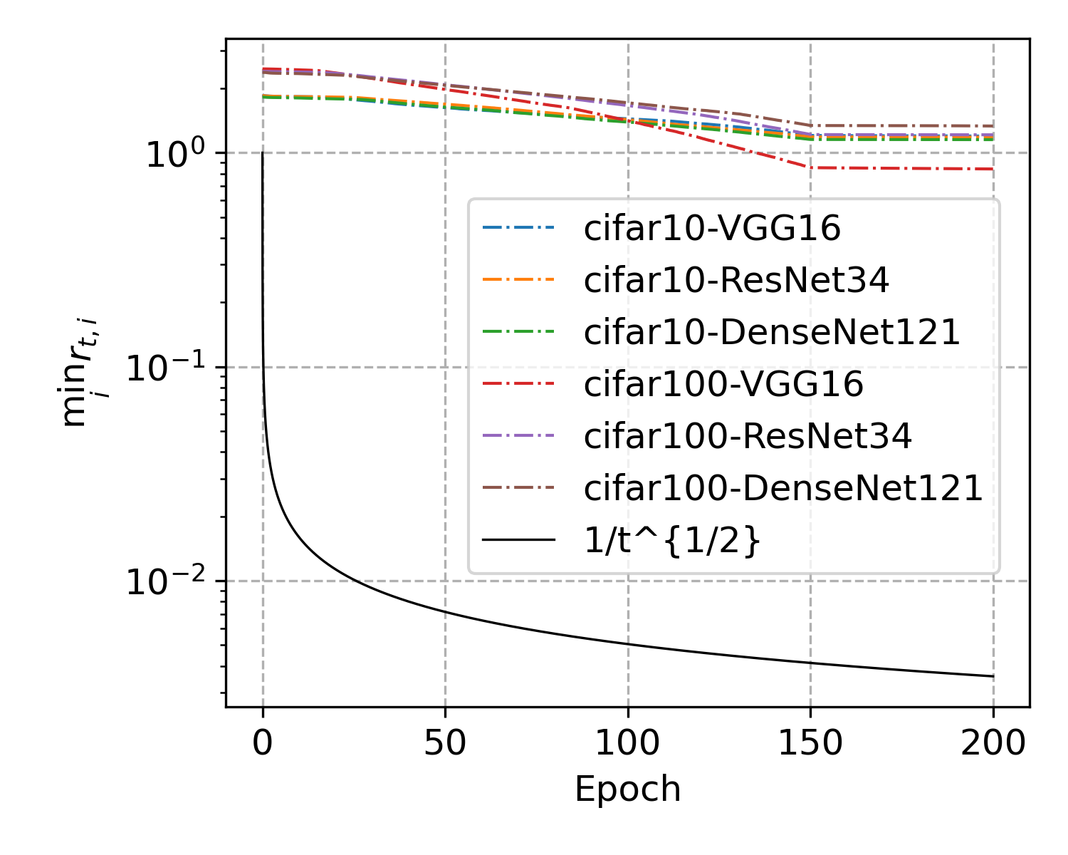
Figure 6. $\min_{i}r_{t,i}$ of AEGDM with default base learning rate $0.01$ in neural network tasks.

(i) The regret bound in (4.3) and the bound in Theorem 4.6 may be seen as a posteriori results due to their dependence on the energy variable $r$ at the $T$-th iteration. These bounds can be useful in planning a learning rate decay schedule based on the updated $r_{t}$. If $r^{*}_{i}>0$, then $R(T)$ is of order $O(\sqrt{T})$, which is known the best possible bound for online convex optimization [9, Section 3.2]. $r^{*}_{i}>0$ is shown to be conditionally true in the stochastic setting (Theorem 4.7). We observe from experimental results (See Figure 6 in Appendix G) that $r_{t,i}$ decays slowly at rate of $t^{-\alpha}$ with $0<\alpha<\frac{1}{2}$ (an algebraic decay rate) for large $t$ with $\eta$ within a reasonable range. In such case, the upper bound of $R(T)$ is of order $O(T^{\frac{\alpha+1}{2}})$. This still ensures the convergence in the sense that

$$\lim_{T\to\infty}\frac{R(T)}{T}=0.$$

It would be of interest to further investigate when this might fail.
(ii) The bound on $\theta_{t}$ is typically enforced by projection onto $\Theta$ [48], with which the regret bound (4.3) can still be proven since projection is a contraction operator [9, Chapter 3].

4.2. Stochastic setting

We proceed to present theoretical results for AEGDM (3.3) in the stochastic setting. Our aim is at solving the following stochastic nonconvex optimization problem

$$\min_{\theta\in\mathbb{R}^{n}}\left\{f(\theta):=\mathbb{E}_{\xi}[f(\theta;\xi)]\right\},$$

where $\xi$ is a random variable satisfying certain distribution, and $f(\theta;\xi):\mathbb{R}^{n}\to\mathbb{R}$ is a differentiable nonconvex function and bounded from below so that $f(\theta;\xi)+c>0$. In the stochastic setting, one can only get estimators of $f(\theta)$ and its gradient, $f(\theta;\xi)$ and $\nabla f(\theta;\xi)$, respectively, with which we take $v_{t}=\nabla f(\theta_{t};\xi_{t})/(2\sqrt{f(\theta_{t};\xi_{t})+c})$ in Algorithm 2.

In the stochastic setting, unconditional energy stability and solution properties in Theorem 4.1 may be stated in the following.

Theorem 4.5 (Energy stability and solution properties).

AEGDM (3.3) is unconditionally energy stable in the sense that for any step size $\eta>0$, $\mathbb{E}[r_{t,i}]$ is strictly decreasing and convergent with $\mathbb{E}[r_{t,i}]\to r^{*}_{i}$ as $t\to\infty$. Moreover, we have the following:
(i) for any $\mu<1$ and $\eta>0$,

$$\lim_{t\to\infty}\mathbb{E}[\|\theta_{t+1}-\theta_{t}\|]=0,\quad\sum_{t=0}^{\infty}\mathbb{E}[\|\theta_{t+1}-\theta_{t}\|^{2}]\leq\frac{2\eta n}{(1-\mu)^{2}}(f(\theta_{0})+c);$$ (4.4)

(ii) for any $\eta>0$,

$$\frac{1}{T}\sum_{t=0}^{T-1}\mathbb{E}[|v_{t,i}|]\leq\Bigg{(}\frac{\sqrt{f(\theta_{0})+c}}{2}\Bigg{)}^{1/2}\left(\mathbb{E}\left[\frac{1}{\eta Tr_{T,i}}\right]\right)^{1/2},\quad i\in[n].$$ (4.5)

In order to present the convergence rate of AEGDM (3.3), we make assumptions that are commonly used for analyzing the convergence of a stochastic algorithm for nonconvex problems:

Assumption 4.1.

1. Smoothness: The objective function is $L$-smooth: $\forall x,y\in\mathbb{R}^{n}$,

   $$f(y)\leq f(x)+\nabla f(x)^{\top}(y-x)+\frac{L}{2}\|y-x\|^{2}.$$

2. Independent samples: The random samples $\{\xi_{t}\}_{t=1}^{\infty}$ are independent.

3. Unbiasedness: The estimate of the gradient and function value are unbiased:

   $$\mathbb{E}_{\xi_{t}}[\nabla f(\theta_{t};\xi_{t})]=\nabla f(\theta_{t}),\quad\mathbb{E}_{\xi_{t}}[f(\theta_{t};\xi_{t})]=f(\theta_{t}).$$

4. Bounded variance: The variance of the estimator of both gradient and function value satisfy

   $$\mathbb{E}_{\xi_{t}}[\|\nabla f(\theta_{t};\xi_{t})-\nabla f(\theta_{t})\|^{2}_{2}]\leq\sigma^{2}_{g},\quad\mathbb{E}_{\xi_{t}}[|f(\theta_{t};\xi_{t})-f(\theta_{t})|^{2}]\leq\sigma^{2}_{f}.$$

Theorem 4.6 (Convergence rate).

Let $\{\theta_{t}\}$ be the solution sequence generated by AEGDM (3.3) with $f_{t}$ in the form of (3.1) and $\mu<1$, $\eta>0$. Under Assumption 4.1 and assume that the stochastic gradient and function value are bounded such that $\|\nabla f(\theta_{t};\xi_{t})\|\leq G_{\infty}$ and $0<a\leq f(\theta_{t},\xi_{t})+c\leq B$, then for all $T\geq 1$,

$$\frac{1}{T}\mathbb{E}\Bigg{[}\min_{i}r_{T,i}\sum_{t=0}^{T-1}\|\nabla f(\theta_{t})\|^{2}_{2}\Bigg{]}\leq\frac{C_{1}+C_{2}n+C_{3}\sigma_{g}\sqrt{nT}}{\eta T},$$

where $C_{1},C_{2},C_{3}$ are constants depending on $\mu,\eta,L,G_{\infty},a,B,n$ and $f_{0}(\theta_{0})+c$.

The proof and the precise expressions for $C_{1},C_{2},C_{3}$ are deferred to Appendix E.

The question of how $r_{T}$ depends on $T$ is theoretically interesting but subtle to characterize. Numerically we observe that for $\eta$ less than a threshold, $r_{T,i}$ tends either to a positive number ($r^{*}_{i}>0$) or to zero much slower than $1/\sqrt{T}$ (See Figure 6 in Appendix G). The above result is meaningful in both cases. In the case $r^{*}_{i}>0$, the rate of $O(1/\sqrt{T})$ is recovered from this bound. Next we shall identify a sufficient condition for ensuring such lower positive threshold for $r_{T,i}$.

4.3. Lower bound of the energy

First note that the $L$-smoothness of $f(\theta)$ implies the $L_{F}$-smoothness of $F(\theta)=\sqrt{f(\theta)+c}$ with

$$L_{F}=\frac{1}{2\sqrt{f(\theta^{*})+c}}\left(L+\frac{G^{2}_{\infty}}{2(f(\theta^{*})+c)}\right).$$ (4.6)

This will be used in our analysis of the asymptotic behavior of the energy. The result is stated below.

Theorem 4.7 (Lower bound of $r_{T}$).

Under the same assumptions as in Theorem 4.6, we have

$$\min_{i}\mathbb{E}[r_{T,i}]\geq\max\{\sqrt{f(\theta^{*})+c}-\eta D_{1}-\mu D_{2}-\sigma D_{3},0\}$$ (4.7)

where $\sigma=\max\{\sigma_{f},\sigma_{g}\}$, with $L_{F}$ given in (4.6) and

$$D_{1}=\frac{L_{F}n(f(\theta_{0})+c)}{(1-\mu)^{2}},\quad D_{2}=\frac{1}{2}\bigg{(}1+\frac{1}{(1-\mu)^{2}}\bigg{)}n\sqrt{f(\theta_{0})+c},$$

$$D_{3}=\frac{1}{2a^{1/2}}+\sqrt{\frac{G_{\infty}^{2}}{4a^{3}}+\frac{1}{a}}\frac{\sqrt{f(\theta_{0})+c}}{1-\mu}\sqrt{\eta nT}.$$

Moreover, in the absence of noise, we have

$$\min_{i}r_{T,i}>\min_{i}r^{*}_{i}>0\quad\text{if}\quad\eta D_{1}+\mu D_{2}<\sqrt{f(\theta^{*})+c}.$$ (4.8)

The derivation of $L_{F}$ and the proof for Theorem 4.7 are deferred to Appendix F.

Remark 4.8.

1. (4.8) is only a sufficient condition. We observe from our experimental results that the upper bound for $\eta$ to guarantee the positiveness of $r^{*}_{i}$ can be much larger (See Figure 6 in Appendix G).

2. In Theorem 4.7, we measure how far $r^{*}$ can deviate from $F(\theta^{*})$ in the worst situation. In the case of no momentum and no noise, we have

$$\min_{i}r_{T,i}>\min_{i}r^{*}_{i}>0\quad\text{if}\quad\eta<\frac{\sqrt{f(\theta^{*})+c}}{D_{1}}.$$

This recovers the result in [21] for the deterministic AEGD.

5. Numerical experiments

In this section, we empirically evaluate AEGDM and compare it with SGDM, Adam, and AEGD on several benchmark problems. We show that in the deterministic case, AEGDM does speed up the convergence of AEGD; in the stochastic case like training deep neural network tasks, the fluctuation of test accuracy of AEGDM is much smaller than that of AEGD (which confirms that AEGDM reduces the variance of AEGD), while AEGDM still achieves comparable final generalization performance of AEGD, which is as well as or better than SGDM. Adam makes rapid initial progress but does not generalize well at the end as the other three methods.

We begin with testing the deterministic counterpart of the method on the 2D-Rosenbrock function, then we conduct the stochastic version on several image classification tasks, including three datasets: MNIST, CIFAR-10 & CIFAR-100 [18]; and six convolution neural network architectures: LeNet-5 [19], VGG-16 [38], ResNet-32 [10], DenseNet-121 [11], SqueezeNet [12], GoogleNet [40]. We choose these architectures because of their broad importance and superior performance on several benchmark tasks.

In all experiments, we set the parameter $c=1$ for both AEGD and AEGDM. The momentum parameter $\mu$ is set to the default value $0.9$ for both SGDM and AEGDM. For Adam, we also directly apply the default hyperparameter values with $\beta_{1}=0.9$ and $\beta_{2}=0.999$. For each method, we only tune the base learning rate. Details about tuning learning rate for training deep neural networks are presented in Section 5.2.

5.1. 2D-Rosenbrock function

We first compare AEGDM with AEGD and GD with momentum (GDM) on the 2D-Rosenbrock function defined by

$$f(x_{1},x_{2})=(1-x_{1})^{2}+100(x_{2}-x_{1}^{2})^{2}.$$ (5.1)

For this non-convex function, the global minimum $f^{*}=0$ achieved at $(1,1)$ is inside a long, narrow, parabolic shaped flag valley. It is trivial to find the valley, but known to be difficult to converge to the global minimum.

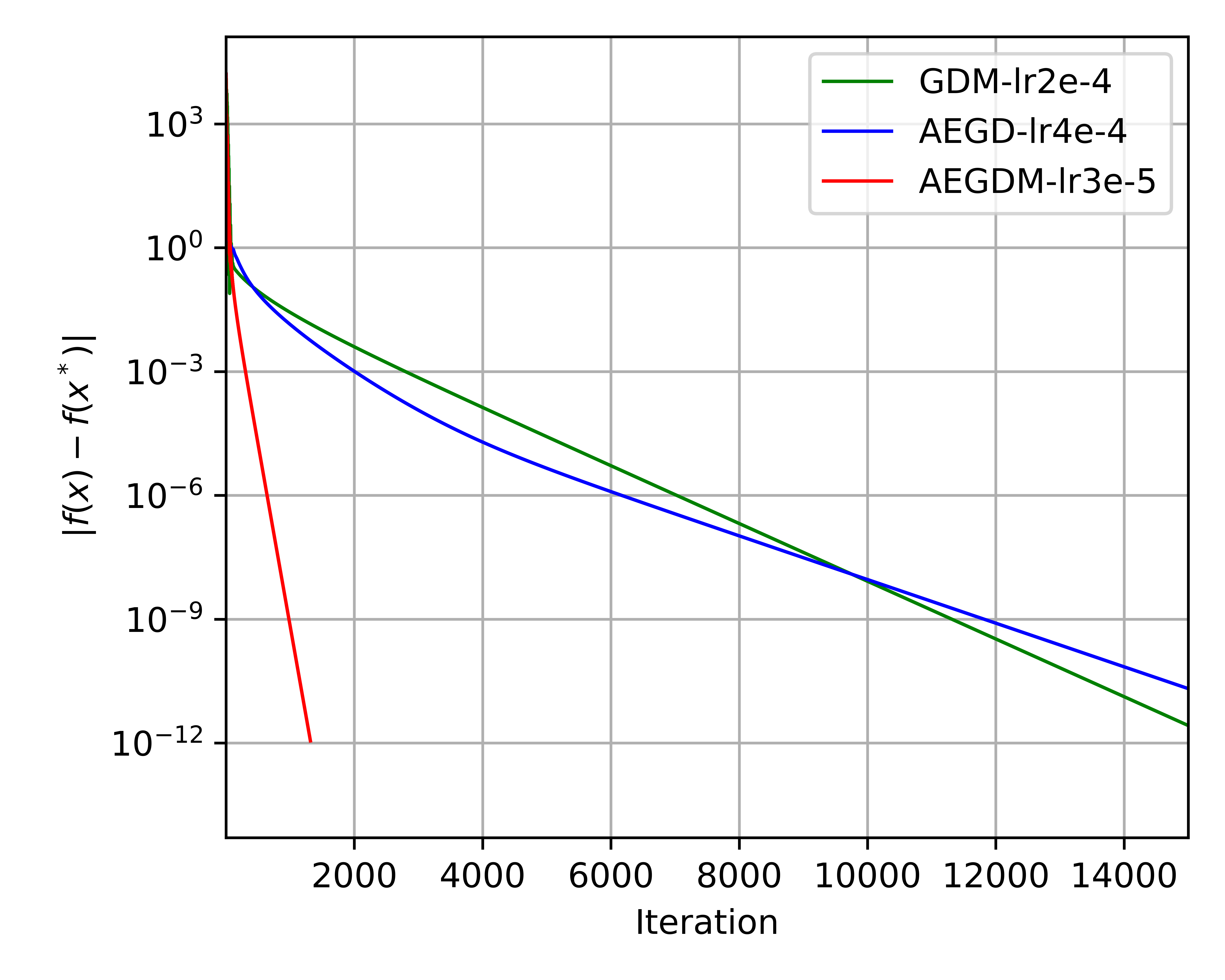
(a) Optimality gap

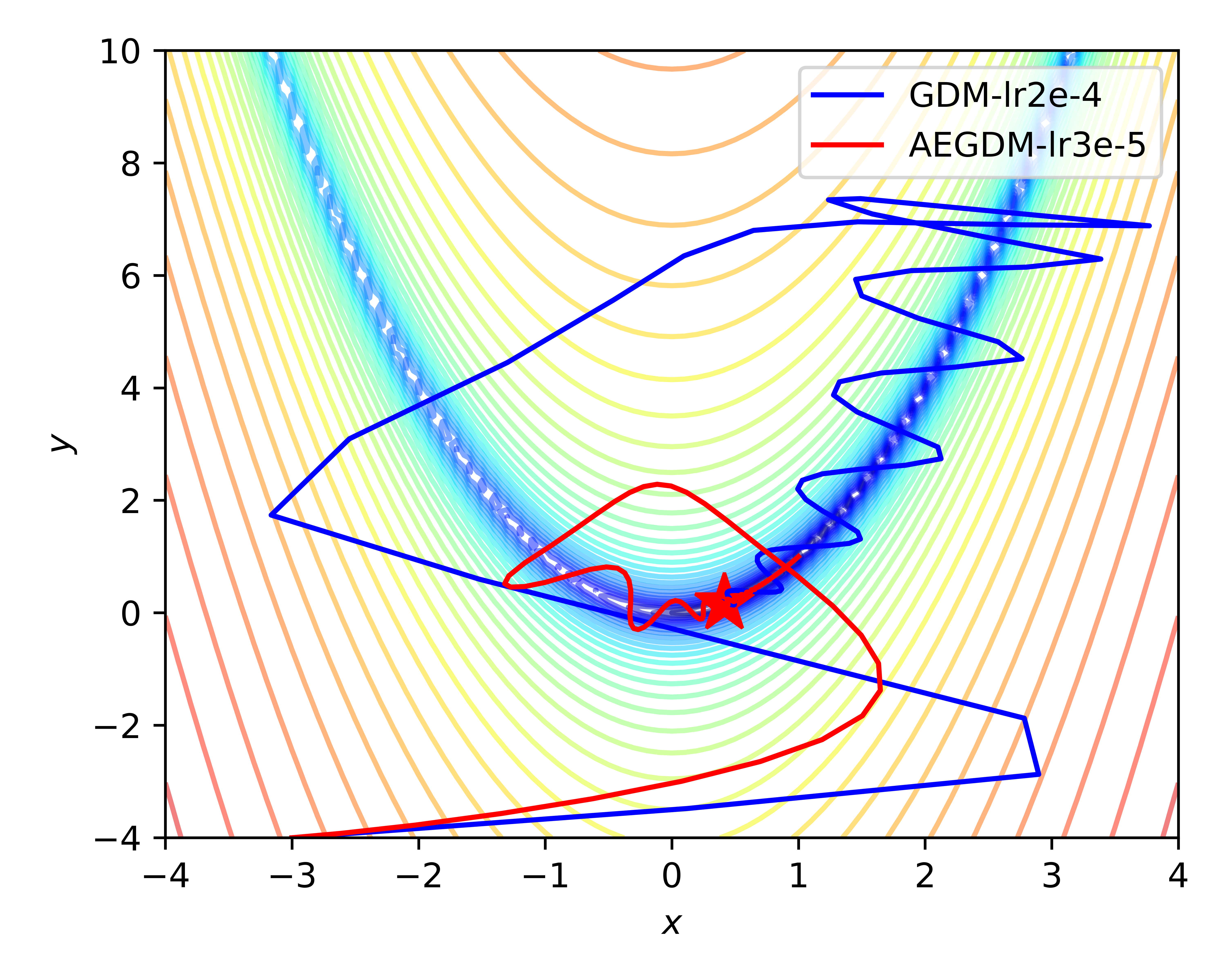
(b) Trajectory

Figure 1. Comparison of the performance of three different methods on the 2D Rosenbrock function.

The initial point is set at $(-3,-4)$. We fine tune the step size and choose the one that achieves the fastest convergence speed for each method. Figure 1 (a) presents the optimality gap v.s. iteration of the three methods, the step size (represented by ‘lr’) used for each method is also included. We see that the performance of AEGD is comparable with that of GDM, and AEGDM converges much faster than both of them. This confirms that momentum can speed up the convergence of AEGD. We also present the trajectory of GDM and AEGDM in Figure 1 (b), it can be seen that though the step size of AEGDM is a lot larger than that of GDM, the oscillation of AEGDM is much smaller, this explains why AEGDM converges much faster than GDM.

5.2. Image classification

Now we compare the performance of AEGDM with SGDM, Adam and AEGD on several image classification tasks, including LeNet-5 on MNIST; VGG-16, ResNet-32, DenseNet-121 on CIFAR-10; and SqueezeNet, GoogleNet on CIFAR-100. For experiments on MNIST, we run $50$ epochs with a minibatch size of $128$ and weight decay of $1\times 10^{-4}$. For experiments on CIFAR-10 and CIFAR-100, we employ the fixed budget of 200 epochs and reduce the learning rates by 10 after 150 epochs. Detailed settings like batch size, and weight decay were chosen as suggested for respective base architectures. We also summarize them in Appendix G.

For each method, we fine tune the base learning rate and report the one that achieves the best final generalization performance. For SGDM, we search the base learning rate $\eta$ among $\{0.01,0.05,0.1,0.2,0.3\}$; for Adam, we search $\eta$ from $\{0.0001,0.0003,0.0005,0.001,0.002\}$; for AEGD, we search $\eta$ from $\{0.05,0.1,0.2,0.3,0.4\}$; for AEGDM, we search $\eta$ from:
$\{0.005,0.008,0.01,0.02,0.03\}$. We found that these choices work well for a wide range of tasks, including examples given below.

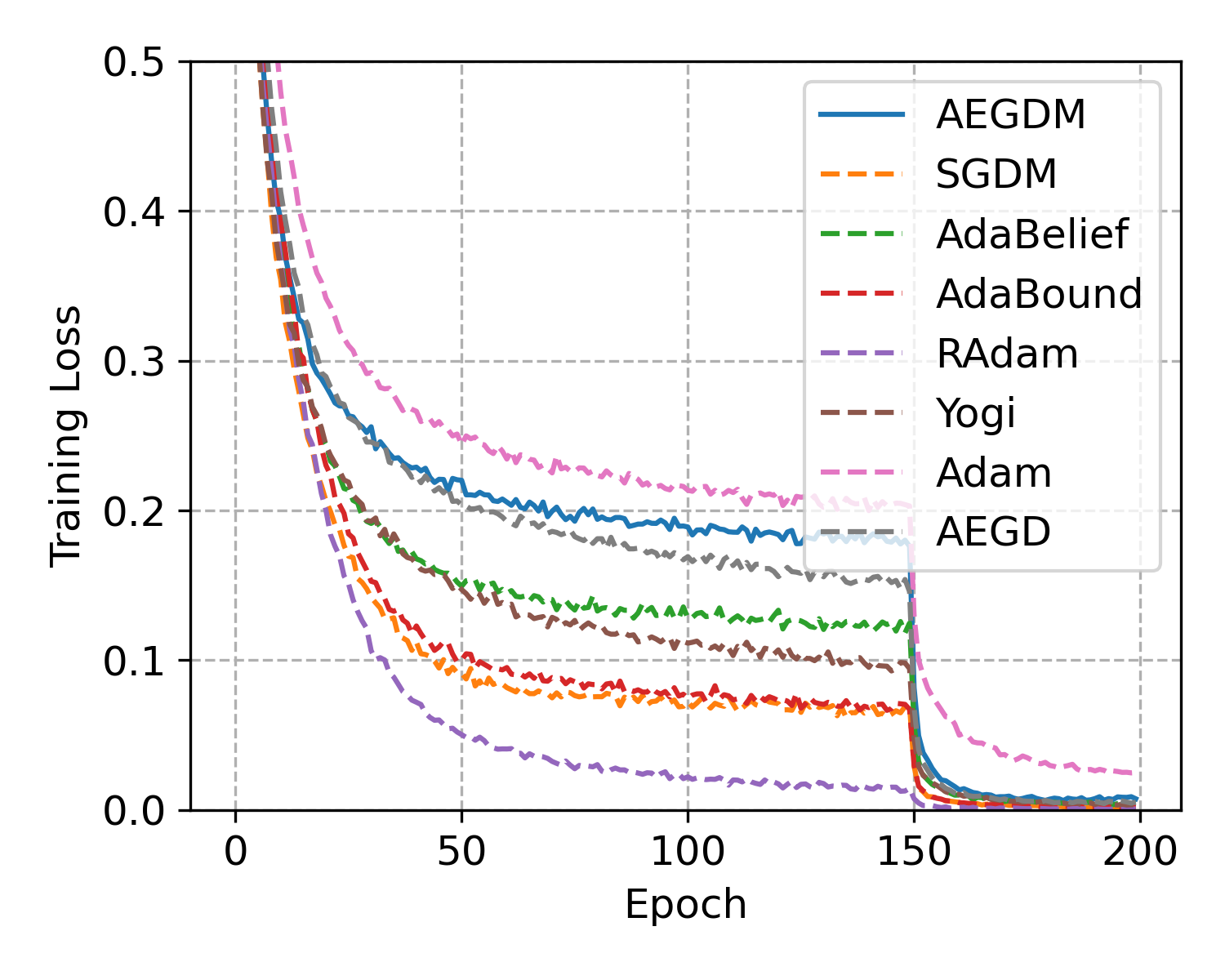
(a) VGG-16, training loss

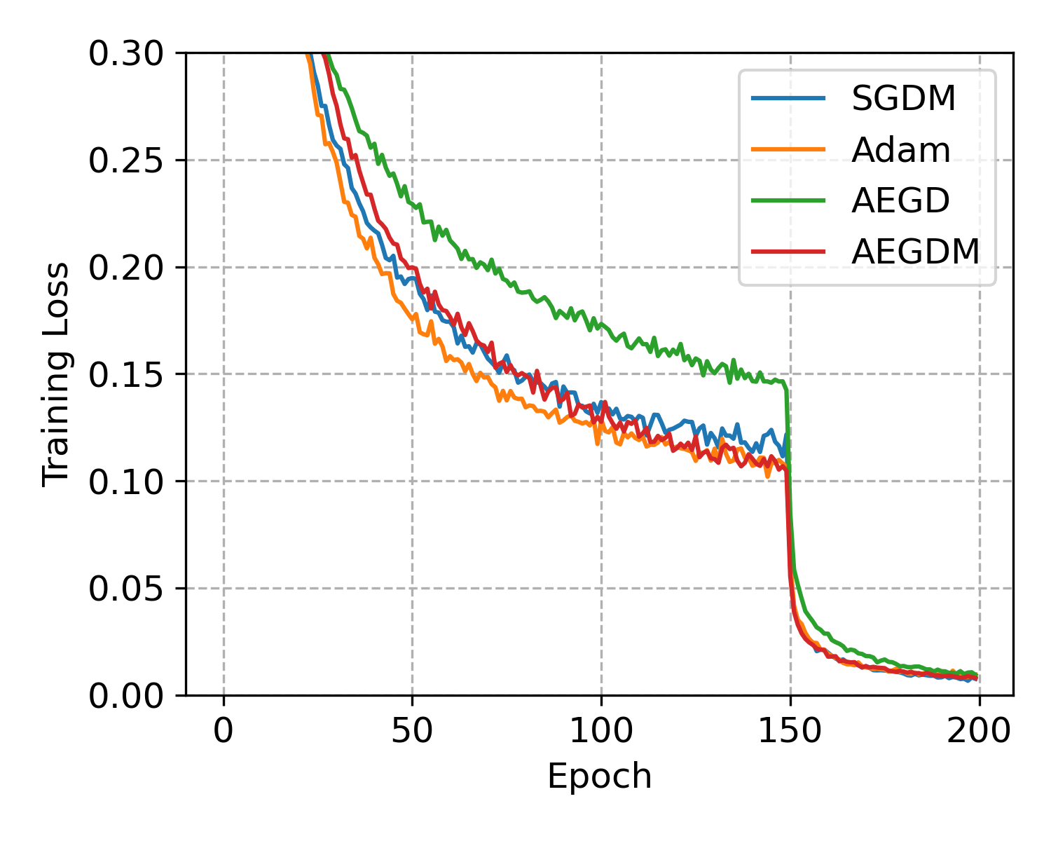
(b) ResNet-32, training loss

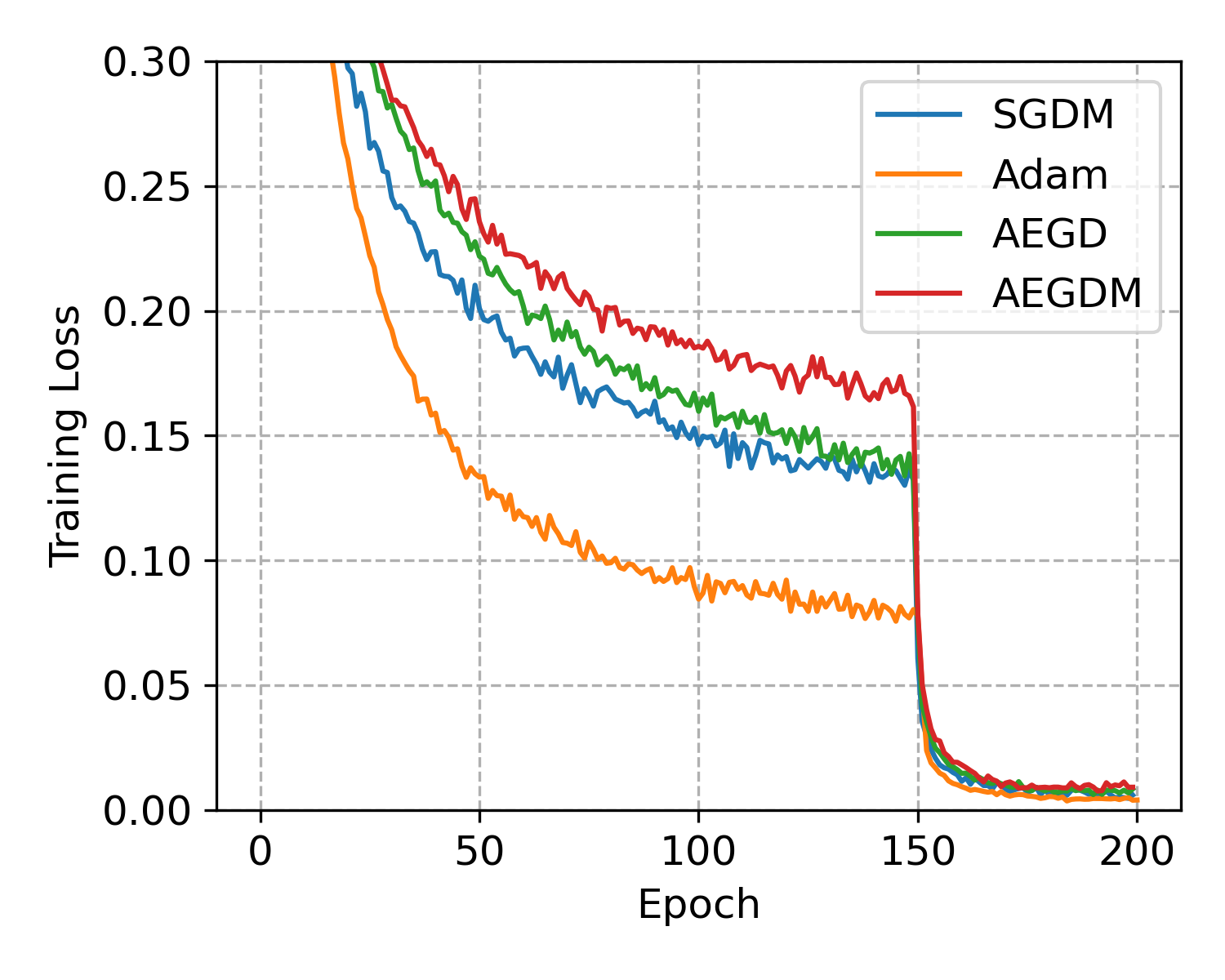
(c) DenseNet-121, training loss

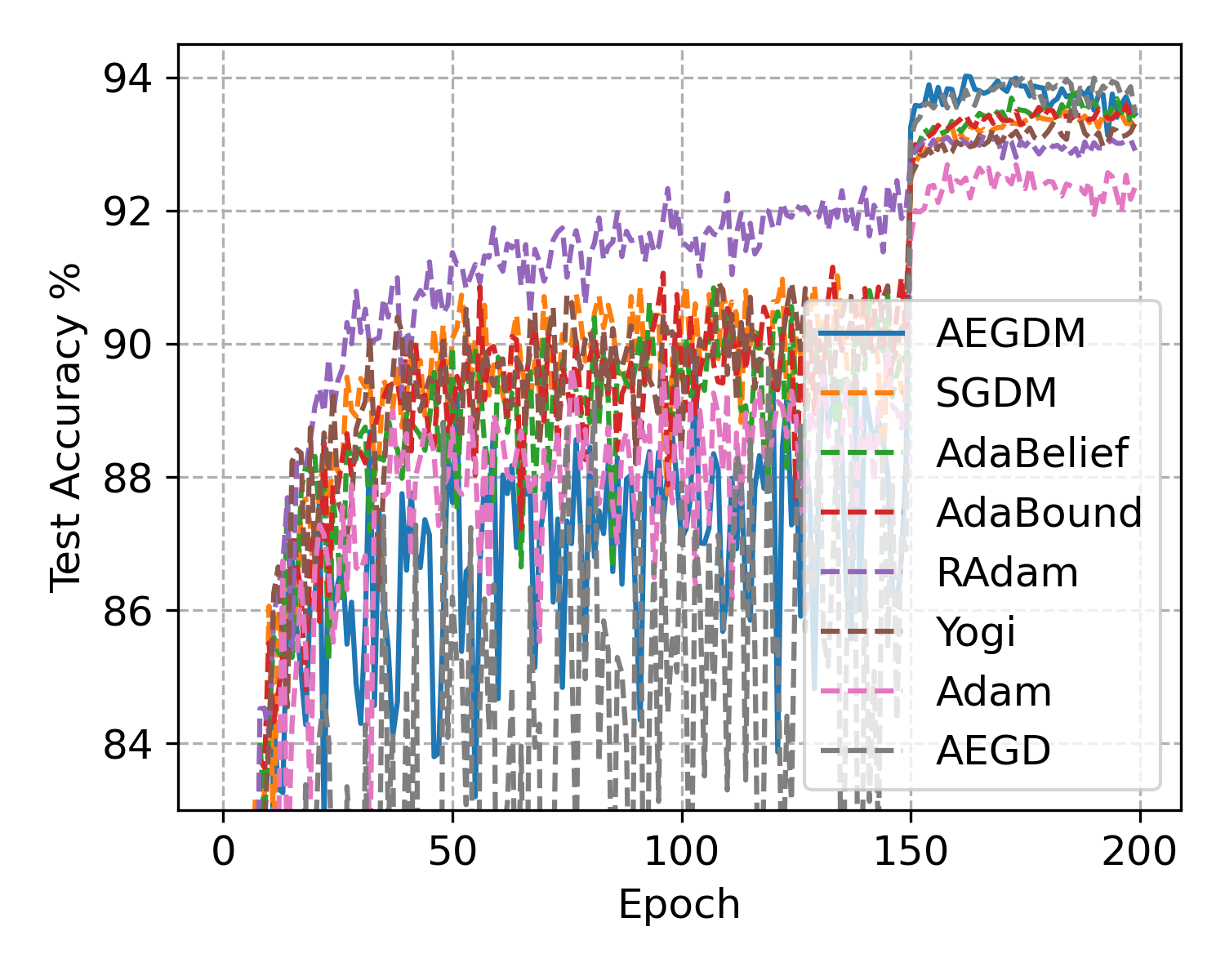
(d) VGG-16, test accuracy

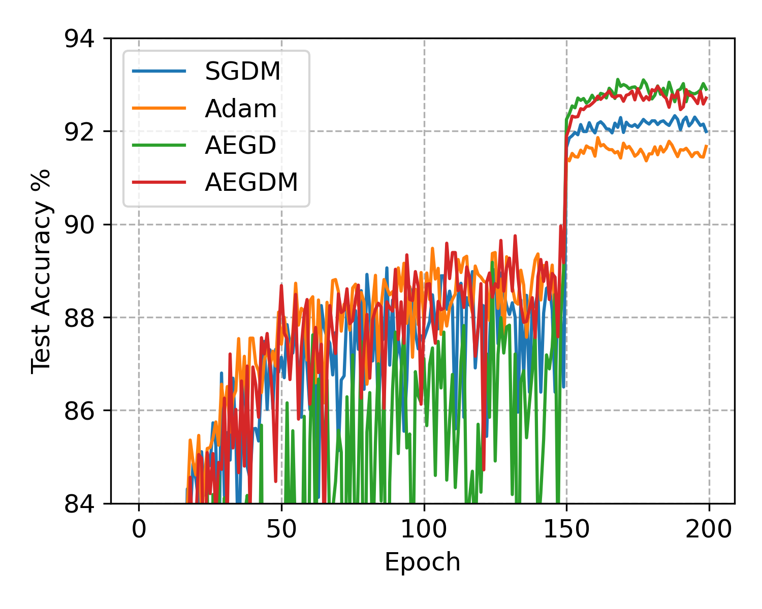
(e) ResNet-32, test accuracy

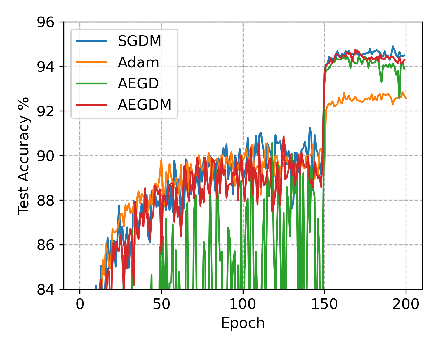
(f) DenseNet-121, test accuracy

Figure 2. Training loss and test accuracy for VGG-16, ResNet-32 and DenseNet-121 on CIFAR-10

MNIST Figure 3 (a) (d) show the training loss and test accuracy against epochs of each method. We see that in the training part, AEGDM and SGDM convergence faster and achieve lower training loss than AEGD and Adam. For test accuracy, we observe an obvious fast initial progress of AEGDM, and it generalizes as well as SGDM at the end. While AEGD and Adam still have small oscillations by epoch 50. In addition, AEGDM gives the highest test accuracy (99.3%) among all the methods.

CIFAR-10 From Figure 2 we can see that the oscillation of AEGD in test accuracy is significantly reduced by AEGDM. Though Adam makes rapid progress in the early stage, the generalization performance of Adam become worse than SGDM, AEGD and AEGDM after epoch 150 when the learning rate decays. In addition, we observe that AEGDM obtain better final generalization performance than SGDM in some tasks. For ResNet-32, AEGDM even surpass SGDM by $\sim 1\%$ in test accuracy.

CIFAR-100 The results are included in Figure 3. We see that the overall performance of each method is similar to that on CIFAR-10. For SqueezeNet, AEGDM gives the highest test accuracy ($71.33\%$) among the four methods. For GoogleNet, AEGD outperforms SGDM by $\sim 0.5\%$ in test accuracy after learning rate decays.

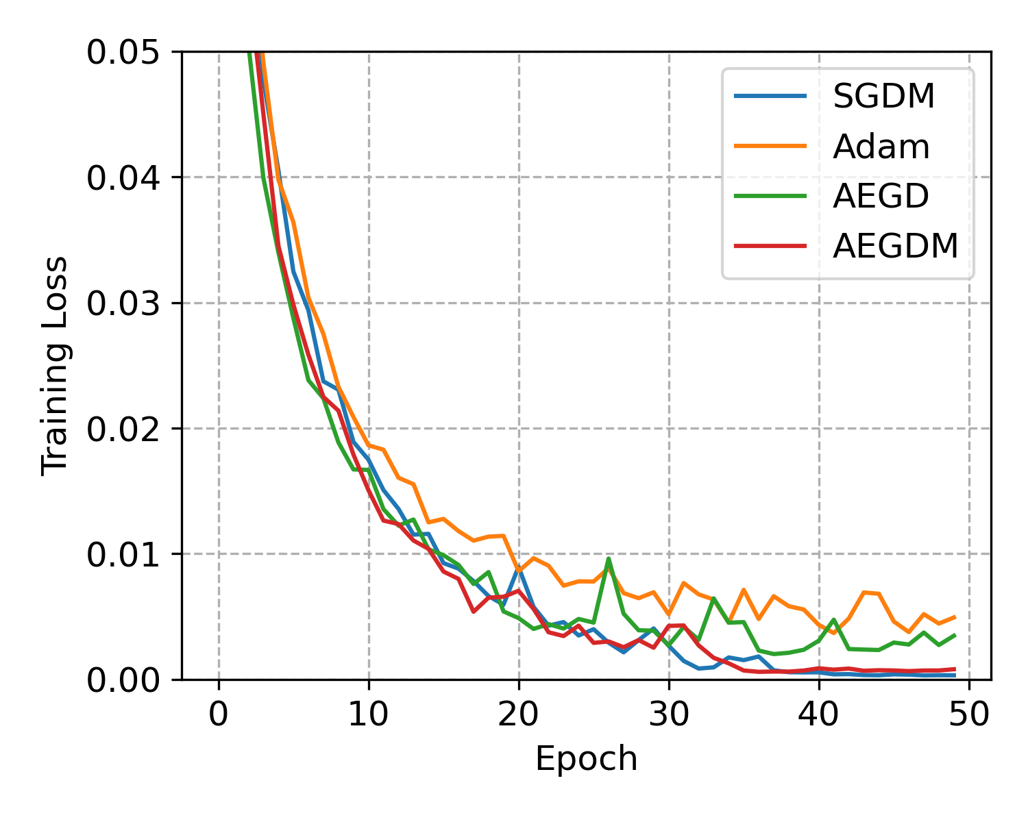
(a) LeNet-5, training loss

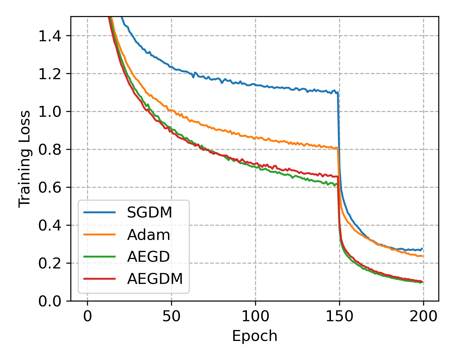
(b) SqueezeNet, training loss

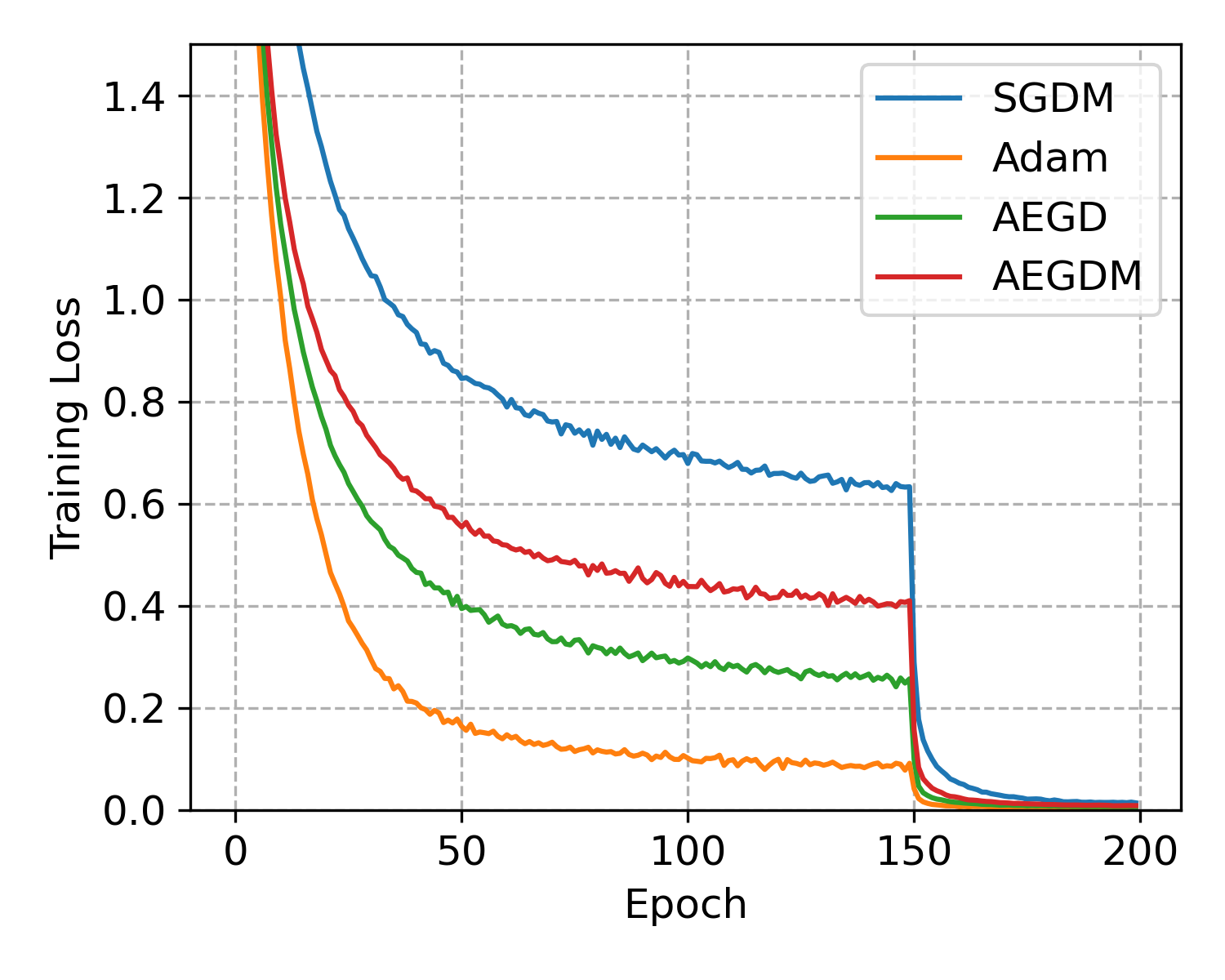
(c) GoogleNet, training loss

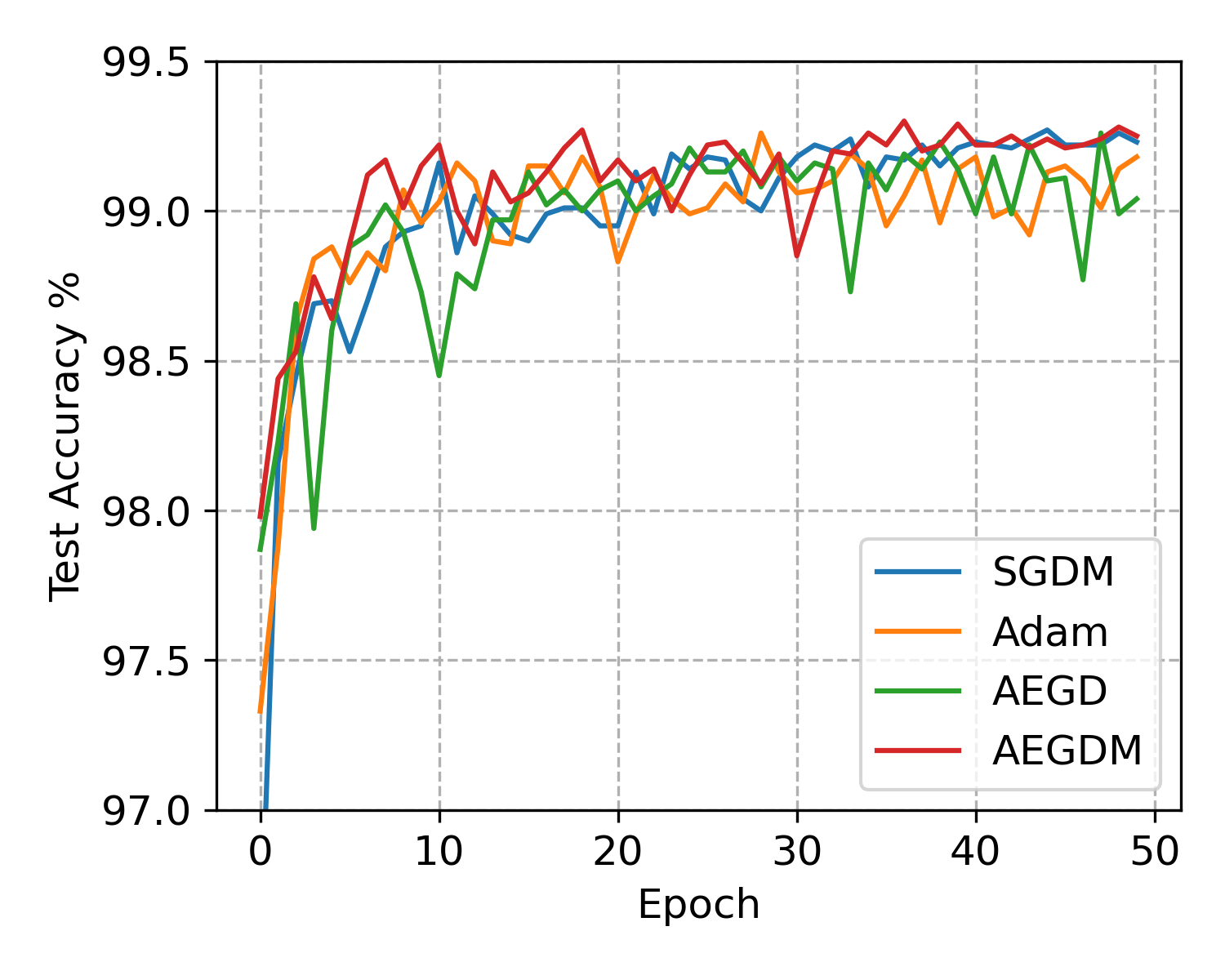
(d) LeNet-5, test accuracy

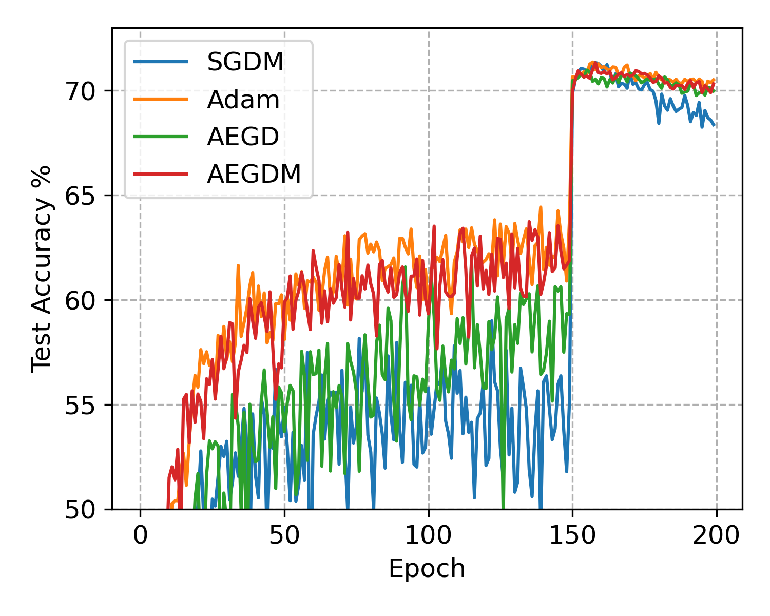
(e) SqueezeNet, test accuracy

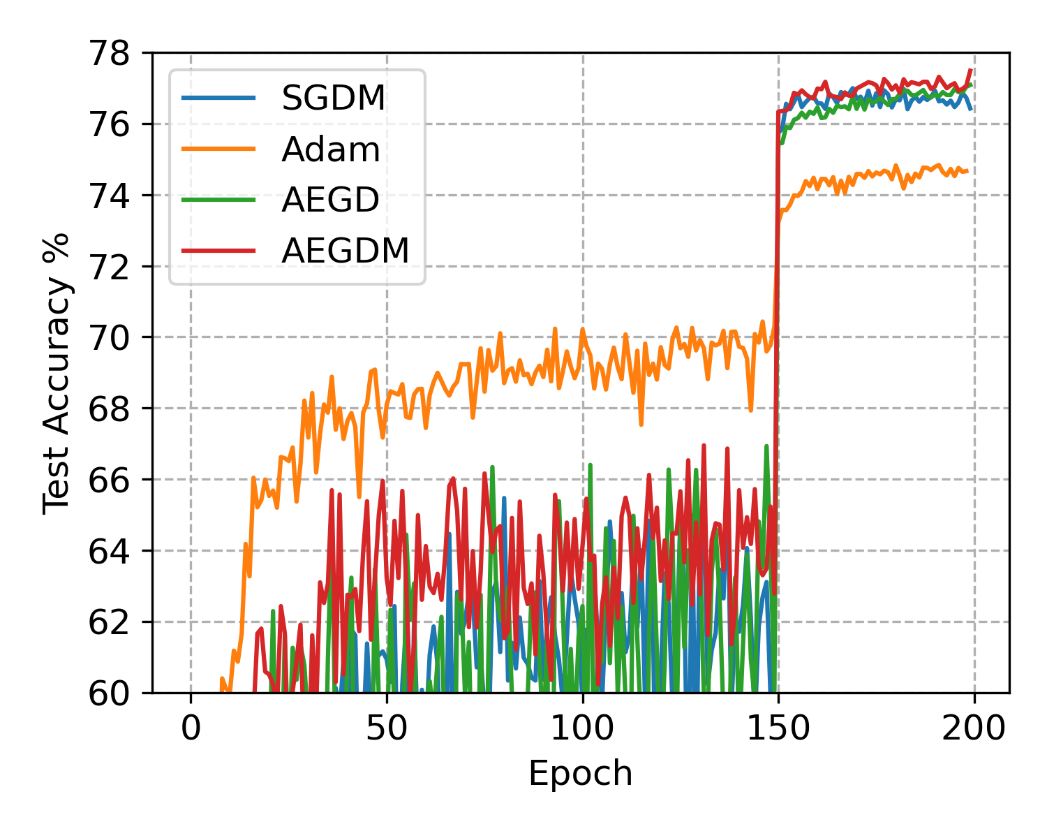
(f) GoogleNet, test accuracy

Figure 3. Training loss and test accuracy for LeNet-5 on MNIST and SqueezeNet, GoogleNet on CIFAR-100

The above results are obtained by fine tuning the base learning rate for each method in each task. While in practice, tuning hyperparameters can be tedious, thus methods require little tuning are more desirable. Therefore, we also conduct comparison (with more methods involved, including AdaBound, AdaBelief, Radam, Yogi) where the default base learning rate is used for each method in all tasks. The results and detailed setting are presented in the Appendix G, from which we see that AEGDM with default base learning rate (0.01) generalizes better than SGDM with default base learning rate (0.1) in all tasks.

6. Discussion

We have developed AEGDM, a gradient method adapted with energy and momentum for solving stochastic optimization problems. The method integrates AEGD introduced in [21] with momentum, featuring unconditional energy stability and guaranteed regret bound. Our experiments show that AEGDM improves AEGD by speeding up the convergence in the deterministic setting and reducing the variance in the stochastic setting. By comparison with SGDM and Adam, we show the potential of AEGD(M) in training deep neural networks to get faster convergence or better generalization performance.

The convergence rates are energy-dependent, hence it is highly desired to obtain sharper estimates on the asymptotic behavior of $r_{t}$ as $t\to\infty$ relative to the base learning rate $\eta$. The result in Theorem 4.7 as an indication of a lower bound for $r_{t}$ is not optimal at all. We expect a positive lower bound for $r_{t}$ at least for small time steps in the deterministic case. This may be seen by analyzing the ODE system obtained from the scheme when the time step tends to zero. In fact, a global version of such system can be derived from (3.3) as

$$\dot{\theta} =-2rm,$$ (6.1a)

$$\dot{r} =-2r|v|^{2},$$ (6.1b)

$$0 =-(1-\mu)m+v,$$ (6.1c)

where $v(s)=\nabla F(\theta(s))$, with $s$ as the continuous time variable, $F(\theta)=\sqrt{f(\theta)+c}$. Observe that

$$\frac{d}{ds}\left[r(s)-(1-\mu)F(\theta(s))\right] =-2r|v|^{2}-(1-\mu)\langle\nabla F(\theta),\dot{\theta}\rangle$$

$$=-2r|v|^{2}-(1-\mu)\langle v,-2rm\rangle=0.$$

Using the choice $r_{0}=F(\theta_{0})$, we obtain

$$r(s)=(1-\mu)F(\theta(s))+\mu F(\theta_{0}).$$

Hence for any $s>0$,

$$r(s)\geq(1-\mu)\min F(\theta)+\mu F(\theta_{0})\geq\min F(\theta)>0.$$

We leave more refined analysis in future work.

Data availability: The data that support the findings of this study are publicly available online at http://yann.lecun.com/exdb/mnist/ and https://www.cs.toronto.edu/~kriz/cifar.html.

In this appendix, we present technical proofs of theoretical results in this work.

Appendix A Auxiliary lemmas and notation

Lemma A.1.

Set $G_{i}(T,\mu)=\sum_{t=1}^{T}r_{t,i}m_{t,i}^{2}$. Then

$$G_{i}(T,\mu)\leq\frac{1}{(1-\mu)^{2}}G_{i}(T,0)$$ (1.1)

provided $\mu<1$.

Proof.

Note that using $m_{0,i}=0$ we may rewrite $G_{i}$ as

$$G_{i}(T,\mu)=\sum_{t=0}^{T}r_{t,i}m_{t,i}^{2}$$

with $G_{i}(0,\mu)=0$. For any $\epsilon>0$ with $(1+\epsilon)\mu^{2}<1$,

$$G_{i}(T,\mu) =\sum_{t=0}^{T-1}r_{t+1,i}m^{2}_{t+1,i}=\sum_{t=0}^{T-1}r_{t+1,i}(\mu m_{t,i}+v_{t,i})^{2}$$

$$\leq\sum_{t=0}^{T-1}((1+\epsilon)\mu^{2}r_{t,i}m_{t,i}^{2}+(1+\epsilon^{-1})r_{t+1,i}v_{t,i}^{2})\qquad(\text{since}\quad r_{t+1,i}\leq r_{t,i})$$

$$\leq(1+\epsilon)\mu^{2}G_{i}(T-1,\mu)+(1+\epsilon^{-1})G_{i}(T,0)$$

$$\leq((1+\epsilon)\mu^{2})^{T}G_{i}(0,\mu)+(1+\epsilon^{-1})G_{i}(T,0)(1+(1+\epsilon)\mu^{2}+\cdots+((1+\epsilon)\mu^{2})^{T-1})$$

$$\leq(1+\epsilon^{-1})G_{i}(T,0)\frac{1}{1-(1+\epsilon)\mu^{2}}.$$

Since $0\leq\mu<1$, we may take $\epsilon=\frac{1-\mu}{\mu}>0$ so that $(1+\epsilon)\mu^{2}=\mu<1$, and $1+\epsilon^{-1}=\frac{1}{1-\mu}$, hence (1.1). ∎

Lemma A.2.

For $0\leq\mu<1$,

$$G_{i}(T,\mu)\leq\frac{r_{0,i}}{2\eta(1-\mu)^{2}}.$$ (1.2)

Proof.

From (3.3c), it follows

$$r_{t,i}-r_{t+1,i}=2\eta r_{t+1,i}v_{t,i}^{2}.$$

Taking summation over $t$ from $0$ to $T-1$ and using telescopic cancellation, we have

$$r_{0,i}-r_{T,i}=2\eta\sum_{t=0}^{T-1}r_{t+1,i}v^{2}_{t,i}.$$

Rearrange the above to get

$$G_{i}(T,0)=\sum_{t=0}^{T-1}r_{t+1,i}v_{t,i}^{2}\leq\frac{r_{0,i}}{2\eta}.$$ (1.3)

By Lemma A.1, we get (1.2). ∎

For the proofs of Theorem 4.1 and 4.3, we introduce notation,

$$F_{t}:=\sqrt{f_{t}(\theta_{t})+c}.$$ (1.4)

The initial data for $r_{i}$ is taken as $r_{0,i}=F_{0}.$ With such choice

$$G(T,\mu)=\sum_{i=1}^{n}G_{i}(T,\mu)\leq\frac{nF_{0}}{2\eta(1-\mu)^{2}}.$$ (1.5)

For the proofs of Theorem 4.5, Theorem 4.6 and Theorem 4.7, we introduce notation

$$\tilde{F}_{t}:=\sqrt{f(\theta_{t};\xi_{t})+c}.$$ (1.6)

The initial data for $r_{i}$ is taken as $r_{0,i}=\tilde{F}_{0}.$ With such choice,

$$G(T,\mu)=\sum_{i=1}^{n}G_{i}(T,\mu)=\frac{n\tilde{F}_{0}}{2\eta(1-\mu)^{2}}.$$ (1.7)

Lemma A.3.

Under the assumptions in Theorem 4.6, we have for all $t\in[T]$,

1. $\|\nabla f(\theta_{t})\|_{\infty}\leq G_{\infty}$.

2. $\mathbb{E}[(\tilde{F}_{t})^{2}]=F^{2}(\theta_{t})=f(\theta_{t})+c$.

3. $\mathbb{E}[\tilde{F}_{t}]\leq F(\theta_{t})$. In particular, $\mathbb{E}[r_{0,i}]=\mathbb{E}[\tilde{F}_{0}]\leq F(\theta_{0})$.

4. $\mathbb{E}[|F(\theta_{t})-\tilde{F}_{t}|]\leq\frac{1}{2a^{1/2}}\sigma_{f}$.

5. $\mathbb{E}[\|\nabla F(\theta_{t})-v_{t}\|^{2}_{2}]\leq\frac{G^{2}_{\infty}}{8a^{3}}\sigma^{2}_{f}+\frac{1}{2a}\sigma^{2}_{g}.$

Proof.

(i) By assumption $\|g_{t}\|_{\infty}\leq G_{\infty}$, we have

$$\|\nabla f(\theta_{t})\|_{\infty}=\|\mathbb{E}[g_{t}]\|_{\infty}\leq\mathbb{E}[\|g_{t}\|_{\infty}]\leq G_{\infty}.$$

(ii) This follows from the unbiased sampling of

$$f(\theta_{t})=\mathbb{E}_{\xi_{t}}[f(\theta_{t};\xi_{t})].$$

(iii) By Jensen’s inequality, we have

$$\mathbb{E}[\tilde{F}_{t}]\leq\sqrt{\mathbb{E}[\tilde{F}_{t}^{2}]}=\sqrt{F(\theta_{t})^{2}}=F(\theta_{t}).$$

(iv) By the assumption $0<a\leq f(\theta_{t};\xi_{t})+c=\tilde{F}_{t}^{2}$, we have

$$\quad\mathbb{E}[|F(\theta_{t})-\tilde{F}_{t}|]\leq\mathbb{E}\Bigg{[}\bigg{|}\frac{f(\theta_{t})-f(\theta_{t};\xi_{t})}{F(\theta_{t})+\tilde{F}_{t}}\bigg{|}\Bigg{]}\leq\frac{1}{2a^{1/2}}\mathbb{E}[|f(\theta_{t})-f(\theta_{t};\xi_{t})|]\leq\frac{1}{2a^{1/2}}\sigma_{f}.$$

(v) By the definition of $F(\theta)$ and $v_{t}$ in (3.3a), we have

$$\|\nabla F(\theta_{t})-v_{t}\|^{2}_{2} =\bigg{\|}\frac{\nabla f(\theta_{t})}{2F(\theta_{t})}-\frac{g_{t}}{2\tilde{F}_{t}}\bigg{\|}^{2}_{2}$$

$$=\frac{1}{4}\bigg{\|}\frac{\nabla f(\theta_{t})(\tilde{F}_{t}-F(\theta_{t}))}{F(\theta_{t})\tilde{F}_{t}}+\frac{\nabla f(\theta_{t})-g_{t}}{\tilde{F}_{t}}\bigg{\|}^{2}_{2}$$

$$\leq\frac{1}{2}\bigg{\|}\frac{\nabla f(\theta_{t})(\tilde{F}_{t}-F(\theta_{t}))}{F(\theta_{t})\tilde{F}_{t}}\bigg{\|}^{2}_{2}+\frac{1}{2}\bigg{\|}\frac{\nabla f(\theta_{t})-g_{t}}{\tilde{F}_{t}}\bigg{\|}^{2}_{2}$$

$$\leq\frac{G^{2}_{\infty}}{2a^{2}}|\tilde{F}_{t}-F(\theta_{t})|^{2}+\frac{1}{2a}\|\nabla f(\theta_{t})-g_{t}\|^{2}_{2},$$

where both the gradient bound and the assumption that $0<a\leq f(\theta_{t};\xi_{t})+c=\tilde{F}^{2}_{t}$ are essentially used. Take an expectation to get

$$\mathbb{E}[\|\nabla F(\theta_{t})-v_{t}\|^{2}_{2}]\leq\frac{G^{2}_{\infty}}{2a^{2}}\mathbb{E}[|\tilde{F}_{t}-F(\theta_{t})|^{2}]+\frac{1}{2a}\mathbb{E}[\|\nabla f(\theta_{t})-g_{t}\|^{2}_{2}].$$

Similar to the proof for ($iv$), we have

$$\mathbb{E}[|\tilde{F}_{t}-F(\theta_{t})|^{2}]\leq\frac{1}{4a}\sigma^{2}_{f}.$$

This together with the variance assumption for $g_{t}$ gives

$$\mathbb{E}[\|\nabla F(\theta_{t})-v_{t}\|^{2}_{2}]\leq\frac{G^{2}_{\infty}}{8a^{3}}\sigma^{2}_{f}+\frac{1}{2a}\sigma^{2}_{g}.$$

∎

Appendix B Proof of Theorem 4.1

The decreasing of $r_{t,i}$ can be easily seen from (3.3c) since $r_{0,i}>0$ and $1+2\eta v^{2}_{t,i}\geq 1$ for all $t\geq 1$ and $i\in[n]$. Using (1.2), we have

$$\quad\sum_{t=0}^{T-1}\|\theta_{t+1}-\theta_{t}\|^{2}_{2} =\sum_{i=1}^{n}\sum_{t=0}^{T-1}(-2\eta r_{t+1,i}m_{t+1,i})^{2}$$

$$\leq 4\eta^{2}\sum_{i=1}^{n}\sum_{t=0}^{T-1}r_{0,i}r_{t+1,i}m^{2}_{t+1,i}$$

$$=4\eta^{2}G(T,\mu)F_{0}\leq\frac{2\eta n}{(1-\mu)^{2}}(f_{0}(\theta_{0})+c).$$

Using the Cauchy-Schwarz inequality, we get

$$\quad\sum_{t=0}^{T-1}|v_{t,i}|=\sum_{t=0}^{T-1}\frac{1}{\sqrt{r_{t+1,i}}}\sqrt{r_{t+1,i}}|v_{t,i}|$$

$$\leq\Bigg{(}\sum_{t=0}^{T-1}\frac{1}{r_{t+1,i}}\Bigg{)}^{1/2}\Bigg{(}\sum_{t=0}^{T-1}r_{t+1,i}v_{t,i}^{2}\Bigg{)}^{1/2}$$

$$\leq\Bigg{(}G_{i}(T,0)\Bigg{)}^{1/2}\Bigg{(}\frac{T}{r_{T,i}}\Bigg{)}^{1/2}.$$

The desired estimate (4.2) follows by using (1.3).

Appendix C Proof of Theorem 4.3

By convexity of $f_{t}$, the regret can be bounded by

$$R(T) =\sum_{t=0}^{T-1}f_{t}(\theta_{t})-f_{t}(\theta^{*})\leq\sum_{t=0}^{T-1}\nabla f_{t}(\theta_{t})^{\top}(\theta_{t}-\theta^{*})=\sum_{t=0}^{T-1}\sum_{i=1}^{n}\partial_{i}f_{t}(\theta_{t})(\theta_{t,i}-\theta^{*}_{i}).$$ (3.1)

Using the update rule (3.3), we have for $i\in[n]$,

$$\theta_{t+1,i}=\theta_{t,i}-2\eta r_{t+1,i}m_{t+1,i}=\theta_{t,i}-2\eta r_{t+1,i}(\mu m_{t,i}+v_{t,i}),$$

which upon subtraction of $\theta^{*}_{i}$ and squaring both sides yields

$$(\theta_{t+1,i}-\theta^{*}_{i})^{2}=(\theta_{t,i}-\theta^{*}_{i})^{2}-4\eta r_{t+1,i}(\mu m_{t,i}+v_{t,i})(\theta_{t,i}-\theta^{*}_{i})+4\eta^{2}r^{2}_{t+1,i}m^{2}_{t+1,i}.$$

Rearranging we get

$$4\eta r_{t+1,i}v_{t,i}(\theta_{t,i}-\theta^{*}_{i})= \Big{(}(\theta_{t,i}-\theta^{*}_{i})^{2}-(\theta_{t+1,i}-\theta^{*}_{i})^{2}\Big{)}-4\eta r_{t+1,i}\mu m_{t,i}(\theta_{t,i}-\theta^{*}_{i})$$

$$+4\eta^{2}r^{2}_{t+1,i}m^{2}_{t+1,i}.$$

Note that $4\eta r_{t+1,i}v_{t,i}=2\eta r_{t+1,i}\partial_{i}f_{t}/F_{t}$, hence the above can be rewritten as

$$\quad\partial_{i}f_{t}(\theta_{t})(\theta_{t,i}-\theta^{*}_{i})$$

$$=\frac{F_{t}}{2\eta r_{t+1,i}}\Big{(}(\theta_{t,i}-\theta^{*}_{i})^{2}-(\theta_{t+1,i}-\theta^{*}_{i})^{2}\Big{)}+2\mu F_{t}m_{t,i}(\theta^{*}_{i}-\theta_{t,i})+2\eta F_{t}r_{t+1,i}m^{2}_{t+1,i}$$

$$=\frac{F_{t}}{2\eta r_{t+1,i}}(\theta_{t,i}-\theta_{t+1,i})\Big{(}(\theta_{t,i}-\theta^{*}_{i})+(\theta_{t+1,i}-\theta^{*}_{i})\Big{)}+2\mu F_{t}m_{t,i}(\theta^{*}_{i}-\theta_{t,i})+2\eta F_{t}r_{t+1,i}m^{2}_{t+1,i}$$

$$=F_{t}m_{t+1,i}\Big{(}(\theta_{t,i}-\theta^{*}_{i})+(\theta_{t+1,i}-\theta^{*}_{i})\Big{)}+2\mu F_{t}m_{t,i}(\theta^{*}_{i}-\theta_{t,i})+2\eta F_{t}r_{t+1,i}m^{2}_{t+1,i}.$$

Using (3.1), we have

$$R(T) \leq\sum_{t=0}^{T-1}\sum_{i=1}^{n}F_{t}m_{t+1,i}\Big{(}(\theta_{t,i}-\theta^{*}_{i})+(\theta_{t+1,i}-\theta^{*}_{i})\Big{)}$$ (3.2)

$$\quad+\sum_{t=0}^{T-1}\sum_{i=1}^{n}2\mu F_{t}m_{t,i}(\theta^{*}_{i}-\theta_{t,i})+\sum_{t=0}^{T-1}\sum_{i=1}^{n}2\eta F_{t}r_{t+1,i}m^{2}_{t+1,i}.$$

Introduce $M(T):=\sum_{t=0}^{T-1}\sum_{i=1}^{n}|m_{t+1,i}|$ and using the bound $F_{t}\leq B^{1/2}$, we can estimate $R(T)$ as follows:

$$R(T) \leq 2B^{1/2}D_{\infty}(M(T)+\mu M(T-1))+2\eta B^{1/2}G(T,\mu)$$

$$\leq 2(1+\mu)B^{1/2}D_{\infty}M(T)+2\eta B^{1/2}G(T,\mu).$$

Note that $G(T,\mu)$ is bounded by (1.5) and $M(T)$ can be bounded by

$$M(T) =\sum_{t=0}^{T-1}\sum_{i=1}^{n}|m_{t+1,i}|$$

$$\leq\left(\sum_{t=0}^{T-1}\sum_{i=1}^{n}r_{t+1,i}|m_{t+1,i}|^{2}\right)^{1/2}\left(\sum_{t=0}^{T-1}\sum_{i=1}^{n}\frac{1}{r_{t+1,i}}\right)^{1/2}$$

$$\leq\sqrt{G(T,\mu)}\left(\sum_{i=1}^{n}\frac{T}{r_{T,i}}\right)^{1/2}.$$

Connecting all the above estimates, we obtain

$$R(T)\leq C_{1}\Bigg{(}\sum_{i=1}^{n}\frac{1}{r_{T,i}}\Bigg{)}^{1/2}\sqrt{T}+C_{2},$$

where

$$C_{1}=2(1+\mu)B^{1/2}D_{\infty}\sqrt{G(T,\mu)},\quad C_{2}=2\eta B^{1/2}G(T,\mu).$$

The regret bound (3.2) follows by using (1.5). This completes the proof of the regret bound.

Appendix D Proof of Theorem 4.5

The proof is entirely similar to the proof of Theorem 4.1, with the use of expectation.

Appendix E Proof of Theorem 4.6

Since $f$ is $L$-smooth, we have

$$f(\theta_{t+1})\leq f(\theta_{t})+\nabla f(\theta_{t})^{\top}(\theta_{t+1}-\theta_{t})+\frac{L}{2}\|\theta_{t+1}-\theta_{t}\|^{2}_{2}.$$ (5.1)

Denoting $\eta_{t}=\eta/\tilde{F}_{t}$, we rewrite the second term in the RHS of (5.1) as

$$\quad\nabla f(\theta_{t})^{\top}(\theta_{t+1}-\theta_{t})$$

$$=\nabla f(\theta_{t})^{\top}(-2\eta r_{t+1}m_{t+1})$$

$$=-2\eta\nabla f(\theta_{t})^{\top}r_{t+1}(\mu m_{t}+v_{t})$$

$$=-2\eta\nabla f(\theta_{t})^{\top}r_{t+1}v_{t}-2\mu\eta\nabla f(\theta_{t})^{\top}r_{t+1}m_{t}$$

$$=-\nabla f(\theta_{t})^{\top}\eta_{t}r_{t+1}g_{t}-2\mu\eta\nabla f(\theta_{t})^{\top}r_{t+1}m_{t}\qquad(\text{since}\quad g_{t}=2\tilde{F}_{t}v_{t})$$

$$=-\nabla f(\theta_{t})^{\top}\eta_{t-1}r_{t}g_{t}+\nabla f(\theta_{t})^{\top}(\eta_{t-1}r_{t}-\eta_{t}r_{t+1})g_{t}-2\mu\eta\nabla f(\theta_{t})^{\top}r_{t+1}m_{t}.$$ (5.2)

We further bound the second term and third term in the RHS of (5.2) separately. For the second term, we have

$$\quad\nabla f(\theta_{t})^{\top}(\eta_{t-1}r_{t}-\eta_{t}r_{t+1})g_{t}$$

$$=\nabla f(\theta_{t})^{\top}\eta_{t-1}(r_{t}-r_{t+1})g_{t}+\nabla f(\theta_{t})^{\top}(\eta_{t-1}-\eta_{t})r_{t+1}g_{t}$$

$$=\nabla f(\theta_{t})^{\top}\eta_{t-1}(r_{t}-r_{t+1})g_{t}+(\eta_{t-1}-\eta_{t})g_{t}^{\top}r_{t+1}g_{t}$$

$$\quad+(\eta_{t-1}-\eta_{t})(\nabla f(\theta_{t})-g_{t})^{\top}r_{t+1}g_{t}$$

$$\leq\eta_{t-1}\|\nabla f(\theta_{t})\|_{\infty}\|r_{t}-r_{t+1}\|_{1,1}\|g_{t}\|_{\infty}+|\eta_{t-1}-\eta_{t}|g_{t}^{\top}r_{t+1}g_{t}$$

$$\quad+|\eta_{t-1}-\eta_{t}|\cdot|(\nabla f(\theta_{t})-g_{t})^{\top}r_{t+1}g_{t}|$$

$$\leq(\eta G^{2}_{\infty}/\sqrt{a})(\|r_{t}\|_{1,1}-\|r_{t+1}\|_{1,1})+(2\eta/\sqrt{a})g_{t}^{\top}r_{t+1}g_{t}$$

$$\quad+(2\eta/\sqrt{a})|(\nabla f(\theta_{t})-g_{t})^{\top}r_{t+1}g_{t}|.$$ (5.3)

The fourth inequality holds because for a positive diagonal matrix $A$, $x^{\top}Ay\leq\|x\|_{\infty}\|A\|_{1,1}\|y\|_{\infty}$, where $\|A\|_{1,1}=\sum_{i}a_{ii}$. The last inequality follows from $r_{t+1,i}\leq r_{t,i}$ for $i\in[n]$ and (i) in Lemma A.3.

For the third term in the RHS of (5.2), we have

$$-2\mu\eta\nabla f(\theta_{t})^{\top}r_{t+1}m_{t} =-2\mu\eta g_{t}^{\top}r_{t+1}m_{t}+2\mu\eta(g_{t}-\nabla f(\theta_{t}))^{\top}r_{t+1}m_{t}$$

$$\leq\mu\eta g_{t}^{\top}r_{t+1}g_{t}+\mu\eta m_{t}^{\top}r_{t+1}m_{t}+2\mu\eta|(g_{t}-\nabla f(\theta_{t}))^{\top}r_{t+1}m_{t}|,$$ (5.4)

where the inequality follows from that for a positive diagonal matrix $A$, $x^{\top}Ay\leq\frac{1}{2}x^{\top}Ax+\frac{1}{2}y^{\top}Ay$. Connecting (5.3) and (5.4), we can further bound (5.2) by

$$\nabla f(\theta_{t})^{\top}(\theta_{t+1}-\theta_{t}) \leq-\nabla f(\theta_{t})^{\top}\eta_{t-1}r_{t}g_{t}+(\eta G^{2}_{\infty}/\sqrt{a})(\|r_{t}\|_{1,1}-\|r_{t+1}\|_{1,1})$$ (5.5)

$$\quad+(2\eta/\sqrt{a}+\mu\eta)g_{t}^{\top}r_{t+1}g_{t}+\mu\eta m_{t}^{\top}r_{t+1}m_{t}$$

$$\quad+(2\eta/\sqrt{a})|(\nabla f(\theta_{t})-g_{t})^{\top}r_{t+1}g_{t}|+2\mu\eta|(g_{t}-\nabla f(\theta_{t}))^{\top}r_{t+1}m_{t}|.$$

Substituting (5.5) into (5.1) and rearranging to get

$$\nabla f(\theta_{t})^{\top}\eta_{t-1}r_{t}g_{t} \leq(f(\theta_{t})-f(\theta_{t+1}))+(\eta G^{2}_{\infty}/\sqrt{a})(\|r_{t}\|_{1,1}-\|r_{t+1}\|_{1,1})$$

$$\quad+(2\eta/\sqrt{a}+\mu\eta)g_{t}^{\top}r_{t+1}g_{t}+\mu\eta m_{t}^{\top}r_{t+1}m_{t}$$

$$\quad+(2\eta/\sqrt{a})|(\nabla f(\theta_{t})-g_{t})^{\top}r_{t+1}g_{t}|+2\mu\eta|(g_{t}-\nabla f(\theta_{t}))^{\top}r_{t+1}m_{t}|$$

$$\quad+\frac{L}{2}\|\theta_{t+1}-\theta_{t}\|^{2}_{2}.$$

Taking an conditional expectation on $(\theta_{t},r_{t})$, we have

$$\quad\nabla f(\theta_{t})^{\top}\eta_{t-1}r_{t}\nabla f(\theta_{t})=\mathbb{E}_{\xi_{t}}\bigg{[}\nabla f(\theta_{t})^{\top}\eta_{t-1}r_{t}g_{t}\bigg{]}$$ (5.6)

$$\leq\mathbb{E}_{\xi_{t}}\Bigg{[}(f(\theta_{t})-f(\theta_{t+1}))+(\eta G^{2}_{\infty}/\sqrt{a})(\|r_{t}\|_{1,1}-\|r_{t+1}\|_{1,1})$$

$$\quad\quad+(2\eta/\sqrt{a}+\mu\eta)g_{t}^{\top}r_{t+1}g_{t}+\mu\eta m_{t}^{\top}r_{t+1}m_{t}$$

$$\quad\quad+(2\eta/\sqrt{a})|(\nabla f(\theta_{t})-g_{t})^{\top}r_{t+1}g_{t}|+2\mu\eta|(g_{t}-\nabla f(\theta_{t}))^{\top}r_{t+1}m_{t}|$$

$$\quad\quad+\frac{L}{2}\|\theta_{t+1}-\theta_{t}\|^{2}_{2}\Bigg{]},$$

where the assumption $\mathbb{E}_{\xi_{t}}[g_{t}]=\nabla f(\theta_{t})$ is used in the first equality. Since $\xi_{1},...,\xi_{t}$ are independent random variables, we set $\mathbb{E}=\mathbb{E}_{\xi_{1}}\mathbb{E}_{\xi_{2}}...\mathbb{E}_{\xi_{T}}$ and take a summation on (5.6) over $t$ from 0 to $T-1$ to get

$$\quad\mathbb{E}\Bigg{[}\sum_{t=0}^{T-1}\nabla f(\theta_{t})^{\top}\eta_{t-1}r_{t}\nabla f(\theta_{t})\Bigg{]}$$ (5.7)

$$\leq\mathbb{E}\Big{[}f(\theta_{0})-f(\theta_{T})\Big{]}+(\eta G^{2}_{\infty}/\sqrt{a})\mathbb{E}\Big{[}\|r_{0}\|_{1,1}-\|r_{T}\|_{1,1}\Big{]}$$

$$\quad+(2\eta/\sqrt{a}+\mu\eta)\mathbb{E}\Bigg{[}\sum_{t=0}^{T-1}g_{t}^{\top}r_{t+1}g_{t}\Bigg{]}+\mu\eta\mathbb{E}\Bigg{[}\sum_{t=0}^{T-1}m_{t}^{\top}r_{t+1}m_{t}\Bigg{]}$$

$$\quad+(2\eta/\sqrt{a})\mathbb{E}\Bigg{[}\sum_{t=0}^{T-1}|(\nabla f(\theta_{t})-g_{t})^{\top}r_{t+1}g_{t}|\Bigg{]}+2\mu\eta\mathbb{E}\Bigg{[}\sum_{t=0}^{T-1}|(g_{t}-\nabla f(\theta_{t}))^{\top}r_{t+1}m_{t}|\Bigg{]}$$

$$\quad+\frac{L}{2}\mathbb{E}\Bigg{[}\sum_{t=0}^{T-1}\|\theta_{t+1}-\theta_{t}\|^{2}_{2}\Bigg{]}.$$

Below we bound each term in (5.7) separately. First recall $g_{t}=2v_{t}\sqrt{f(\theta_{t};\xi_{t})+c}$, and $f(\theta_{t};\xi_{t})+c\leq B$, we have

$$\sum_{t=0}^{T-1}g_{t}^{\top}r_{t+1}g_{t}\leq 4B\sum_{t=0}^{T-1}v_{t}^{\top}r_{t+1}v_{t}=4BG(T,0)\leq 2nB\tilde{F}_{0}/\eta,$$

where (1.7) with $\mu=0$ was used. Note that by $r_{t+1,i}\leq r_{t,i}$, we have

$$\sum_{t=0}^{T-1}m_{t}^{\top}r_{t+1}m_{t}\leq\sum_{t=0}^{T-1}m_{t}^{\top}r_{t}m_{t}=\sum_{t=0}^{T-2}m_{t+1}^{\top}r_{t+1}m_{t+1}\leq G(T,\mu)\leq\frac{n\tilde{F}_{0}}{2\eta(1-\mu)^{2}},$$

where (1.7) was used. These two bounds allow us to further get

$$\sum_{t=0}^{T-1}\|r_{t+1}g_{t}\|^{2}_{2} =\sum_{i=1}^{n}\sum_{t=0}^{T-1}r^{2}_{t+1,i}g_{t,i}^{2}\leq\sum_{i=1}^{n}\sum_{t=0}^{T-1}r_{0,i}r_{t+1,i}g_{t,i}^{2}$$

$$=\bigg{(}\sum_{i=1}^{n}\sum_{t=0}^{T-1}r_{t,i}g_{t,i}^{2}\bigg{)}\tilde{F}_{0}\leq 2nB\tilde{F}^{2}_{0}/\eta,$$ (5.8)

and also

$$\sum_{t=0}^{T-1}\|r_{t+1}m_{t}\|^{2}_{2}\leq\bigg{(}\sum_{i=1}^{n}\sum_{t=0}^{T-1}r_{t,i}m_{t,i}^{2}\bigg{)}\tilde{F}_{0} \leq\frac{n\tilde{F}^{2}_{0}}{2\eta(1-\mu)^{2}}.$$ (5.9)

For the rest three terms in (5.7), we use the Cauchy-Schwarz inequality to get

$$\mathbb{E}\Bigg{[}\sum_{t=0}^{T-1}|(g_{t}-\nabla f(\theta_{t}))^{\top}r_{t+1}m_{t}|\Bigg{]} \leq\mathbb{E}\Bigg{[}\sum_{t=0}^{T-1}\|\nabla f(\theta_{t})-g_{t}\|_{2}\|r_{t+1}m_{t}\|_{2}\Bigg{]}$$

$$\leq\mathbb{E}\Bigg{[}\bigg{(}\sum_{t=0}^{T-1}\|\nabla f(\theta_{t})-g_{t}\|^{2}_{2}\bigg{)}^{1/2}\bigg{(}\sum_{t=0}^{T-1}\|r_{t+1}m_{t}\|^{2}_{2}\bigg{)}^{1/2}\Bigg{]}$$

$$\leq\Bigg{(}\mathbb{E}\Bigg{[}\sum_{t=0}^{T-1}\|\nabla f(\theta_{t})-g_{t}\|^{2}_{2}\Bigg{]}\Bigg{)}^{1/2}\Bigg{(}\mathbb{E}\Bigg{[}\sum_{t=0}^{T-1}\|r_{t+1}m_{t}\|^{2}_{2}\Bigg{]}\Bigg{)}^{1/2}$$

$$\leq\sigma_{g}\sqrt{nT/2\eta}F(\theta_{0})/(1-\mu),$$ (5.10)

where (5.9) and the bounded variance assumption were used. We replace $m_{t}$ in (5.10) by $g_{t}$ and use (5.8) to get

$$\mathbb{E}\Bigg{[}\sum_{t=1}^{T}|(\nabla f(\theta_{t})-g_{t})^{\top}r_{t+1}g_{t}|\Bigg{]} \leq\Bigg{(}\mathbb{E}\Bigg{[}\sum_{t=0}^{T-1}\|\nabla f(\theta_{t})-g_{t}\|^{2}_{2}\Bigg{]}\Bigg{)}^{1/2}\Bigg{(}\mathbb{E}\Bigg{[}\sum_{t=0}^{T-1}\|r_{t+1}g_{t}\|^{2}_{2}\Bigg{]}\Bigg{)}^{1/2}$$

$$\leq\sigma_{g}\sqrt{2BnT/\eta}F(\theta_{0}).$$ (5.11)

By (4.4), the last term in (5.7) is bounded above by

$$\frac{L}{2}\mathbb{E}\left[\sum_{t=0}^{\infty}\|\theta_{t+1}-\theta_{t}\|^{2}\right]\leq\frac{L\eta n}{(1-\mu)^{2}}F^{2}(\theta_{0}).$$ (5.12)

Substituting (5.11), (5.10), (5.12) into (5.7), using Lemma A.3, $\mathbb{E}[\|r_{0}\|_{1,1}]\leq nF(\theta_{0})$, we get

$$\mathbb{E}\Bigg{[}\sum_{t=0}^{T-1} \nabla f(\theta_{t})^{\top}\eta_{t-1}r_{t}\nabla f(\theta_{t})\Bigg{]}\leq(f(\theta_{0})-f(\theta^{*}))+\eta n(G^{2}_{\infty}/\sqrt{a})F(\theta_{0})$$ (5.13)

$$+\Big{(}4B/\sqrt{a}+2\mu B+\mu/(2(1-\mu)^{2})\Big{)}nF(\theta_{0})$$

$$+(2\sqrt{2B/a}+\sqrt{2}\mu/(1-\mu))\sigma_{g}\sqrt{\eta nT}F(\theta_{0})+L\eta nF^{2}(\theta_{0})/(1-\mu)^{2}.$$

Note that the left hand side is bounded from below by

$$\eta B^{-1/2}\mathbb{E}\Bigg{[}\min_{i}r_{T,i}\sum_{t=0}^{T-1}\|\nabla f(\theta_{t})\|^{2}_{2}\Bigg{]},$$

where we used $\eta_{t}\geq\eta/B^{1/2}$. Thus we have

$$\mathbb{E}\Bigg{[}\min_{i}r_{T,i}\sum_{t=0}^{T-1}\|\nabla f(\theta_{t})\|^{2}_{2}\Bigg{]}\leq\frac{C_{1}+C_{2}n+C_{3}\sigma_{g}\sqrt{nT}}{\eta},$$

where

$$C_{1} =(f(\theta_{0})-f(\theta^{*}))B^{1/2},$$

$$C_{2} =\Big{(}\eta G^{2}_{\infty}/\sqrt{a}+4B/\sqrt{a}+2\mu B+\mu/(2(1-\mu)^{2})\Big{)}B^{1/2}\sqrt{f(\theta_{0})+c}$$

$$\quad+\eta LB^{1/2}(f(\theta_{0})+c)/(1-\mu)^{2},$$

$$C_{3} =\big{(}2\sqrt{B/a}+\mu/(1-\mu)\big{)}\sqrt{2\eta B}\sqrt{f(\theta_{0})+c}.$$

Appendix F Proof of Theorem 4.7

Recall that $F(\theta)=\sqrt{f(\theta)+c}$, then for any $x,y\in\{\theta_{t}\}_{t=0}^{T}$ we have

$$\|\nabla F(x)-\nabla F(y)\| =\bigg{\|}\frac{\nabla f(x)}{2F(x)}-\frac{\nabla f(y)}{2F(y)}\bigg{\|}$$

$$=\frac{1}{2}\bigg{\|}\frac{\nabla f(x)(F(y)-F(x))}{F(x)F(y)}+\frac{\nabla f(x)-\nabla f(y)}{F(y)}\bigg{\|}$$

$$\leq\frac{G_{\infty}}{2(F(\theta^{*}))^{2}}|F(y)-F(x)|+\frac{1}{2F(\theta^{*})}\|\nabla f(x)-\nabla f(y)\|.$$

One may check that

$$|F(y)-F(x)|\leq\frac{G_{\infty}}{2F(\theta^{*})}\|x-y\|.$$

These together with the $L$-smoothness of $f$ lead to

$$\|\nabla F(x)-\nabla F(y)\|_{2}\leq L_{F}\|x-y\|,$$

where

$$L_{F}=\frac{1}{2\sqrt{f(\theta^{*})+c}}\left(L+\frac{G^{2}_{\infty}}{2(f(\theta^{*})+c)}\right).$$

This confirms the $L_{F}$-smoothness of $F$, which yields

$$F(\theta_{t+1})-F(\theta_{t}) \leq\nabla F(\theta_{t})^{\top}(\theta_{t+1}-\theta_{t})+\frac{L_{F}}{2}\|\theta_{t+1}-\theta_{t}\|^{2}$$

$$=(\nabla F(\theta_{t})-v_{t})^{\top}(\theta_{t+1}-\theta_{t})+v_{t}^{\top}(\theta_{t+1}-\theta_{t})+\frac{L_{F}}{2}\|\theta_{t+1}-\theta_{t}\|^{2}.$$

Summation of the above over $t$ from $0$ to $T-1$ and taken with the expectation gives

$$\mathbb{E}[F(\theta_{T})-F(\theta_{0})]\leq\sum_{i=1}^{3}S_{i},$$ (6.1)

where

$$S_{1}=\mathbb{E}\Bigg{[}\sum_{t=0}^{T-1}v_{t}^{\top}(\theta_{t+1}-\theta_{t})\Bigg{]},$$

$$S_{2}=\mathbb{E}\Bigg{[}\sum_{t=0}^{T-1}(\nabla F(\theta_{t})-v_{t})^{\top}(\theta_{t+1}-\theta_{t})\Bigg{]},$$

$$S_{3}=\mathbb{E}\Bigg{[}\sum_{t=0}^{T-1}\frac{L_{F}}{2}\|\theta_{t+1}-\theta_{t}\|^{2}\Bigg{]}.$$

Below we bound $S_{1},S_{2},S_{3}$ separately. To bound $S_{1}$, we first note that

$$r_{t+1,i}-r_{t,i} =-2\eta r_{t+1,i}v^{2}_{t,i}=v_{t,i}(-2\eta r_{t+1,i}v_{t,i})$$

$$=v_{t,i}\big{(}-2\eta r_{t+1,i}(m_{t+1,i}-\mu m_{t,i})\big{)}$$

$$=v_{t,i}\big{(}-2\eta r_{t+1,i}m_{t+1,i}+2\mu\eta r_{t+1,i}m_{t,i}\big{)}$$

$$=v_{t,i}(\theta_{t+1,i}-\theta_{i})+2\mu\eta r_{t+1,i}v_{t,i}m_{t,i},$$

from which we get

$$S_{1} =\mathbb{E}\Bigg{[}\sum_{t=0}^{T-1}v_{t}^{\top}(\theta_{t+1}-\theta_{t})\Bigg{]}$$

$$=\mathbb{E}\Bigg{[}\sum_{i=1}^{n}\sum_{t=0}^{T-1}r_{t+1,i}-r_{t,i}-2\mu\eta r_{t+1,i}v_{t,i}m_{t,i}\Bigg{]}$$

$$=\sum_{i=1}^{n}\mathbb{E}[r_{T,i}]-n\mathbb{E}[\tilde{F}_{0}]-2\mu\eta\mathbb{E}\Bigg{[}\sum_{i=1}^{n}\sum_{t=0}^{T-1}r_{t+1,i}v_{t,i}m_{t,i}\Bigg{]},$$

where the third equality follows from (3.3c).

For $S_{2}$, by Cauchy-Schwarz inequality, we have

$$S_{2} =\mathbb{E}\Bigg{[}\sum_{t=0}^{T-1}(\nabla F(\theta_{t})-v_{t})^{\top}(\theta_{t+1}-\theta_{t})\Bigg{]}$$

$$\leq\mathbb{E}\Bigg{[}\sum_{t=0}^{T-1}\|\nabla F(\theta_{t})-v_{t})\|_{2}\|\theta_{t+1}-\theta_{t})\|_{2}\Bigg{]}$$

$$\leq\mathbb{E}\Bigg{[}\bigg{(}\sum_{t=0}^{T-1}\|\nabla F(\theta_{t})-v_{t})\|^{2}_{2}\bigg{)}^{1/2}\bigg{(}\sum_{t=0}^{T-1}\|\theta_{t+1}-\theta_{t}\|^{2}_{2}\bigg{)}^{1/2}\Bigg{]}$$

$$\leq\Bigg{(}\mathbb{E}\Bigg{[}\sum_{t=0}^{T-1}\|\nabla F(\theta_{t})-v_{t})\|^{2}_{2}\Bigg{]}\Bigg{)}^{1/2}\Bigg{(}\mathbb{E}\Bigg{[}\sum_{t=0}^{T-1}\|\theta_{t+1}-\theta_{t}\|^{2}_{2}\Bigg{]}\Bigg{)}^{1/2}$$

$$\leq\frac{\sqrt{2}F(\theta_{0})}{1-\mu}\sqrt{\eta nT}\sqrt{\frac{G^{2}_{\infty}}{8a^{3}}\sigma^{2}_{f}+\frac{1}{2a}\sigma^{2}_{g}},$$

where the last inequality is by ($v$) in Lemma A.3 and (4.4) in Theorem 4.5.

For $S_{3}$, also by (4.4) in Theorem 4.5, we have

$$S_{3}=\frac{L_{F}}{2}\mathbb{E}\Bigg{[}\sum_{t=0}^{T-1}\|\theta_{t+1}-\theta_{t}\|^{2}\Bigg{]}\leq\frac{L_{F}\eta nF^{2}(\theta_{0})}{(1-\mu)^{2}}.$$

With the above bounds on $S_{1},S_{2},S_{3}$, (6.1) can be rearranged as

$$\quad F(\theta^{*})+2\mu\eta\mathbb{E}\Bigg{[}\sum_{i=1}^{n}\sum_{t=0}^{T-1}r_{t+1,i}v_{t,i}m_{t,i}\Bigg{]}-\frac{L_{F}\eta nF^{2}(\theta_{0})}{(1-\mu)^{2}}-\frac{F(\theta_{0})}{1-\mu}\sqrt{\eta nT}\sqrt{\frac{G^{2}_{\infty}}{4a^{3}}\sigma^{2}_{f}+\frac{1}{a}\sigma^{2}_{g}}$$

$$\leq\sum_{i=1}^{n}\mathbb{E}[r_{T,i}]-n\mathbb{E}[\tilde{F}_{0}]+F(\theta_{0})$$

$$\leq\Big{(}\min_{i}\mathbb{E}[r_{T,i}]+(n-1)\mathbb{E}[\tilde{F}_{0}]\Big{)}-(n-1)\mathbb{E}[\tilde{F}_{0}]+\Big{(}F(\theta_{0})-\mathbb{E}[\tilde{F}_{0}]\Big{)}$$

$$\leq\min_{i}\mathbb{E}[r_{T,i}]+\mathbb{E}[|F(\theta_{0})-\tilde{F}_{0}|]$$

$$\leq\min_{i}\mathbb{E}[r_{T,i}]+\frac{1}{2a^{1/2}}\sigma_{f},$$

where (iii) in Lemma A.3 was used. Hence,

$$\min_{i}\mathbb{E}[r_{T,i}]\geq F(\theta^{*})+2\mu\eta\mathbb{E}\Bigg{[}\sum_{i=1}^{n}\sum_{t=0}^{T-1}r_{t+1,i}v_{t,i}m_{t,i}\Bigg{]}-\eta D_{1}-\sigma D_{3},$$ (6.2)

where $\sigma=\max\{\sigma_{f},\sigma_{g}\}$ and

$$D_{1}=\frac{L_{F}nF^{2}(\theta_{0})}{(1-\mu)^{2}},\quad D_{3}=\frac{1}{2a^{1/2}}+\frac{F(\theta_{0})}{1-\mu}\sqrt{\eta nT}\sqrt{\frac{G^{2}_{\infty}}{4a^{3}}+\frac{1}{a}}.$$

The remaining term in (6.2) with $\mu=0$ vanishes. For $\mu>0$ we proceed to bound this term as follows:

$$\sum_{i=1}^{n}\sum_{t=0}^{T-1}r_{t+1,i}v_{t,i}m_{t,i} \geq-\frac{1}{2}\sum_{i=1}^{n}\sum_{t=0}^{T-1}r_{t+1,i}v^{2}_{t,i}-\frac{1}{2}\sum_{i=1}^{n}\sum_{t=0}^{T-1}r_{t+1,i}m^{2}_{t,i}$$

$$\geq-\frac{1}{2}(G(T,0)+G(T-1,\mu))\geq-\bigg{(}1+\frac{1}{(1-\mu)^{2}}\bigg{)}n\tilde{F}_{0}/(4\eta),$$

which allows us to obtain

$$2\mu\eta\mathbb{E}\Bigg{[}\sum_{i=1}^{n}\sum_{t=0}^{T-1}r_{t+1,i}v_{t,i}m_{t,i}\Bigg{]}\geq-\frac{\mu}{2}\bigg{(}1+\frac{1}{(1-\mu)^{2}}\bigg{)}n\mathbb{E}[\tilde{F}_{0}]\leq-\frac{\mu}{2}\bigg{(}1+\frac{1}{(1-\mu)^{2}}\bigg{)}nF(\theta_{0}).$$

Therefore,

$$\min_{i}\mathbb{E}[r_{T,i}]\geq\max\{\sqrt{f(\theta^{*})+c}-\eta D_{1}-\mu D_{2}-\sigma D_{3},0\},$$

where $\sigma=\max\{\sigma_{f},\sigma_{g}\}$ and

$$D_{1}=\frac{L_{F}n(f(\theta_{0})+c)}{(1-\mu)^{2}},\quad D_{2}=\frac{1}{2}\bigg{(}1+\frac{1}{(1-\mu)^{2}}\bigg{)}n\sqrt{f(\theta_{0})+c},$$

$$D_{3}=\frac{1}{2a^{1/2}}+\frac{\sqrt{f(\theta_{0})+c}}{1-\mu}\sqrt{\eta nT}\sqrt{\frac{G^{2}_{\infty}}{4a^{3}}+\frac{1}{a}}.$$

Appendix G Implementation details of experiments

We summarize the setup for experiments presented in Section 5 in Table 1, where ‘BS’ and ‘WD’ represent batch size and weight decay employed for each task, respectively. The last four columns are base learning rate that achieves the best final generalization performance for each method in respective tasks.

Table 1. Training settings in our experiments

Dataset	Model	BS	WD	SGDM	Adam	AEGD	AEGDM
MNIST	LeNet-5	128	$1e-4$	0.01	0.001	0.05	0.008
CIFAR-10	VGG-16	128	$5e-4$	0.03	0.0003	0.1	0.005
CIFAR-10	ResNet-32	128	$1e-4$	0.05	0.001	0.2	0.008
CIFAR-10	DenseNet-121	64	$1e-4$	0.05	0.0005	0.2	0.02
CIFAR-100	SqueezeNet	128	$1e-4$	0.3	0.003	0.2	0.02
CIFAR-100	GoogleNet	128	$1e-4$	0.2	0.0003	0.2	0.03

Figure 4, 5 present the comparison results where the defaults base learning rate for each method:

• AEGDM: $0.01$.

• AEGD: $0.1$.

• SGDM: $0.01$ for VGG-16 (on both CIFAR10 and CIFAR100), $0.1$ for other tasks.

• AdaBelief, AdaBound, RAdam, Yogi, Adam: $0.001$.

is used in all tasks. Also different from the setting reported in Table 1, here we set batch size as $128$ and weight decay as $5\times 10^{-4}$ in all tasks. It can be seen that AEGDM and AEGD generalize better than all other methods, and AEGD display smaller oscillation / faster convergence than AEGD.

The experiments were coded in PyTorch and conducted using job scheduling on Intel E5-2640 v3 CPU (two 2.6 GHz 8-Core) with 128 GB Memory per Node.

(a) VGG-16, training loss

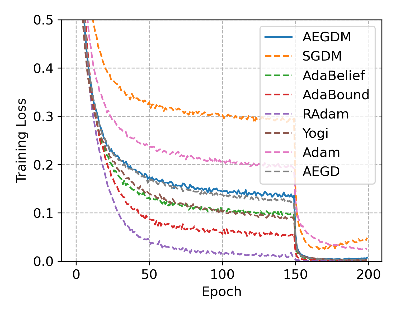
(b) ResNet-34, training loss

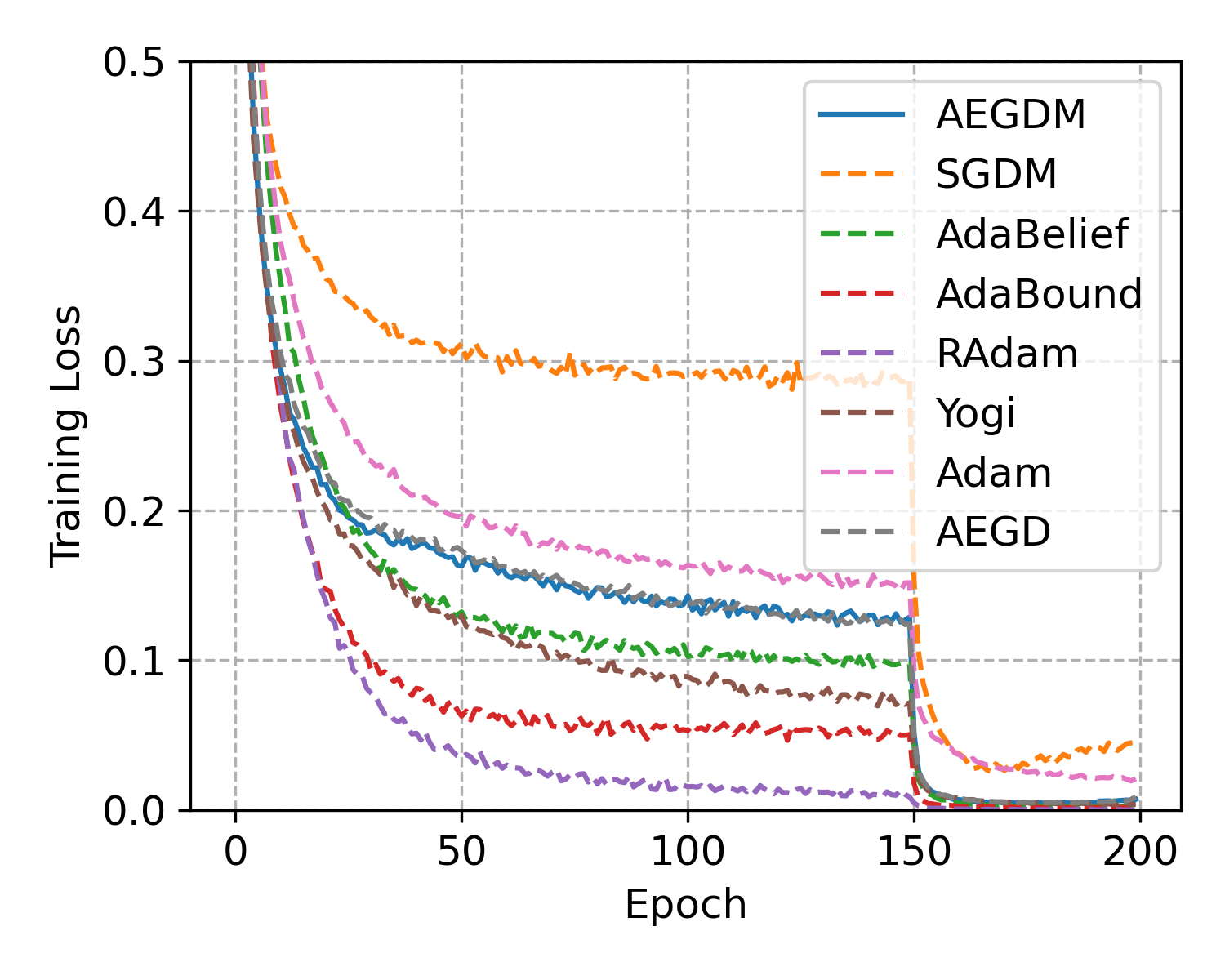
(c) DenseNet-121, training loss

(d) VGG-16, test accuracy

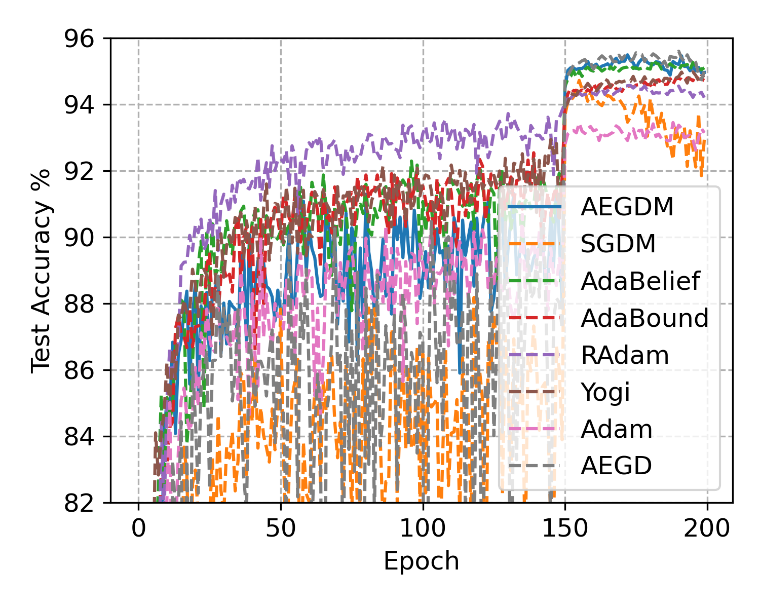
(e) ResNet-34, test accuracy

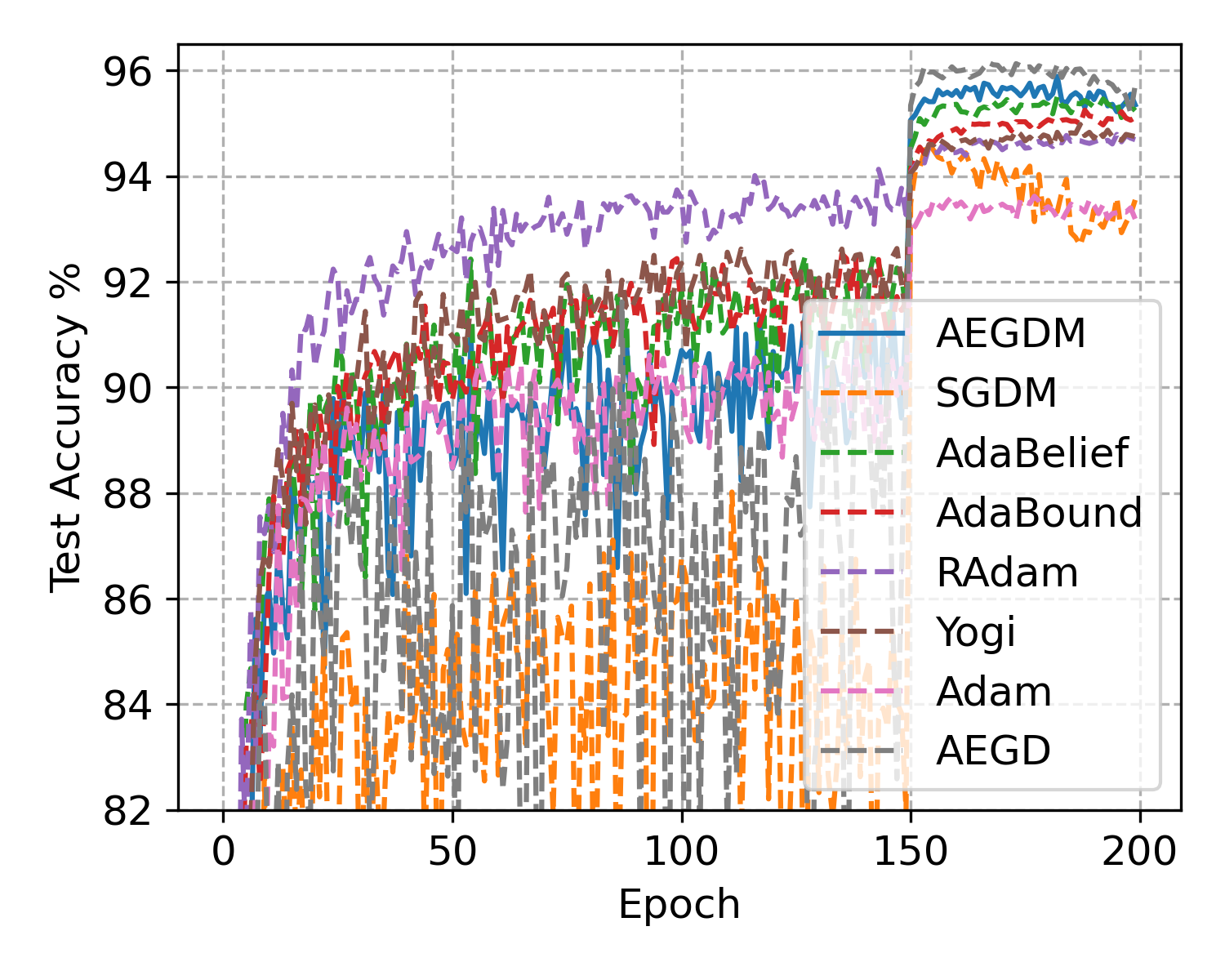
(f) DenseNet-121, test accuracy

Figure 4. Test accuracy for VGG-16, ResNet-34 and DenseNet-121 on CIFAR-10

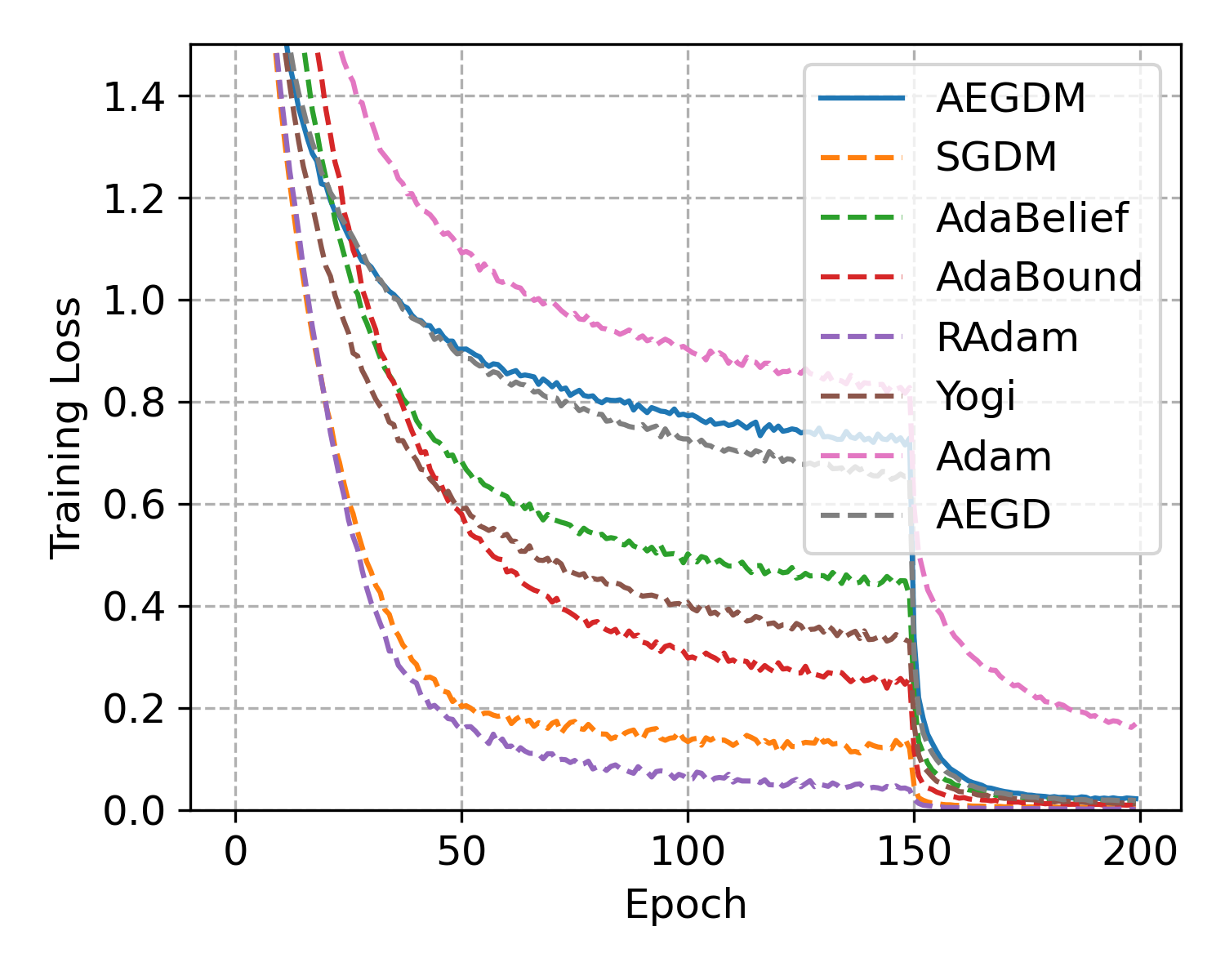
(a) VGG-16, training loss

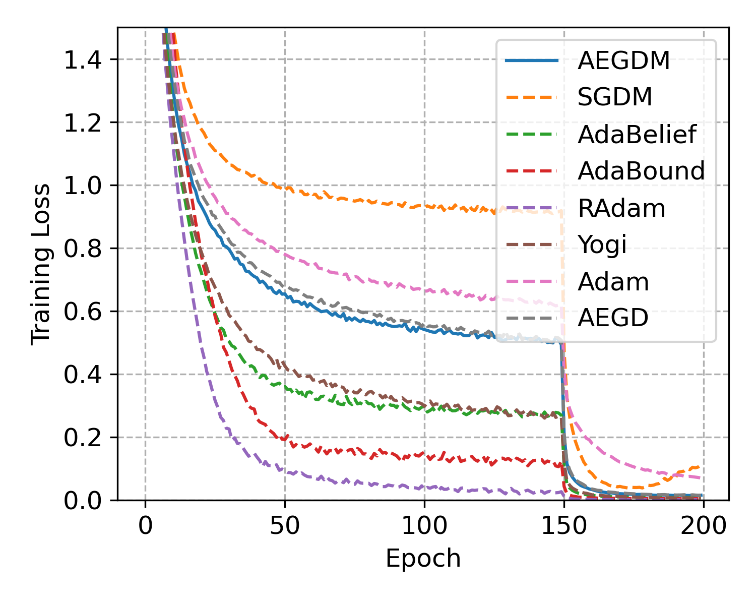
(b) ResNet-34, training loss

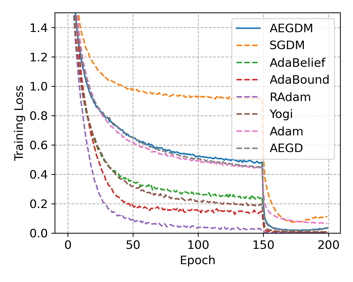
(c) DenseNet-121, training loss

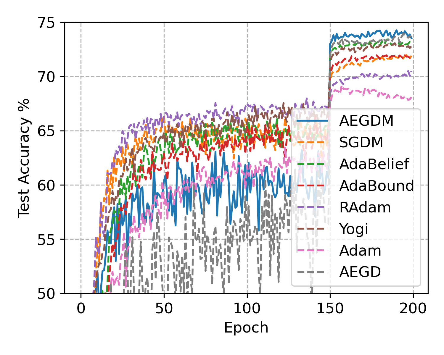
(d) VGG-16, test accuracy

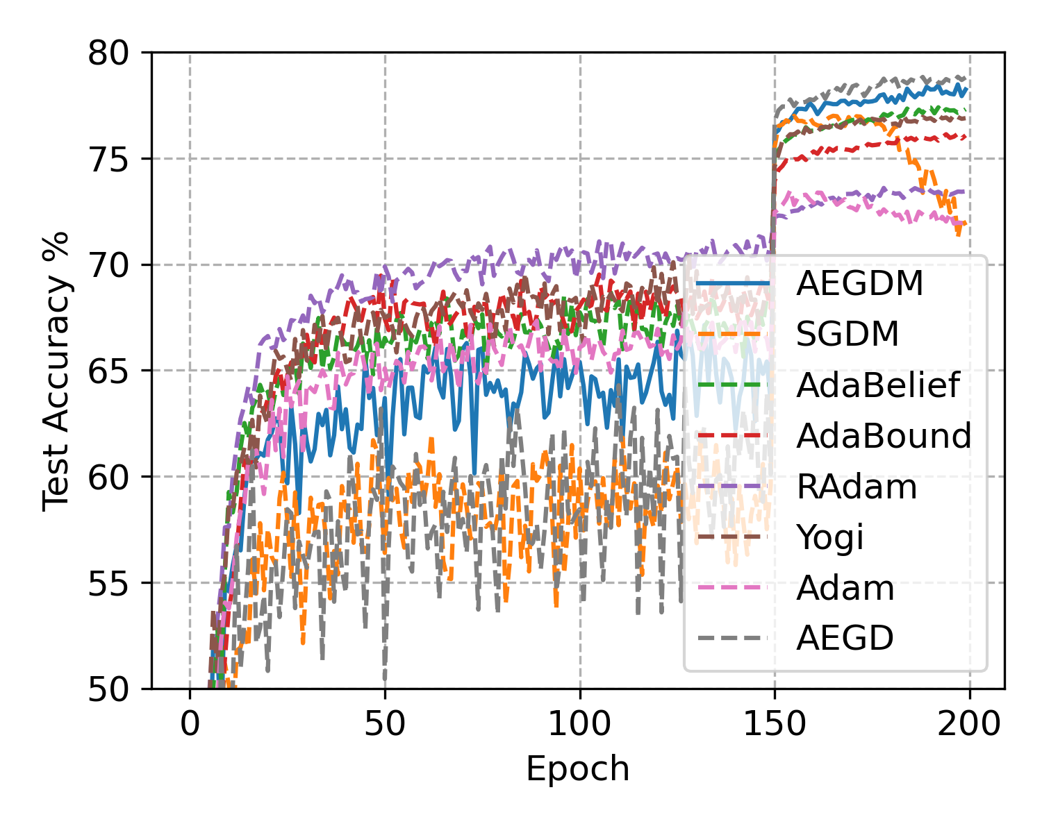
(e) ResNet-34, test accuracy

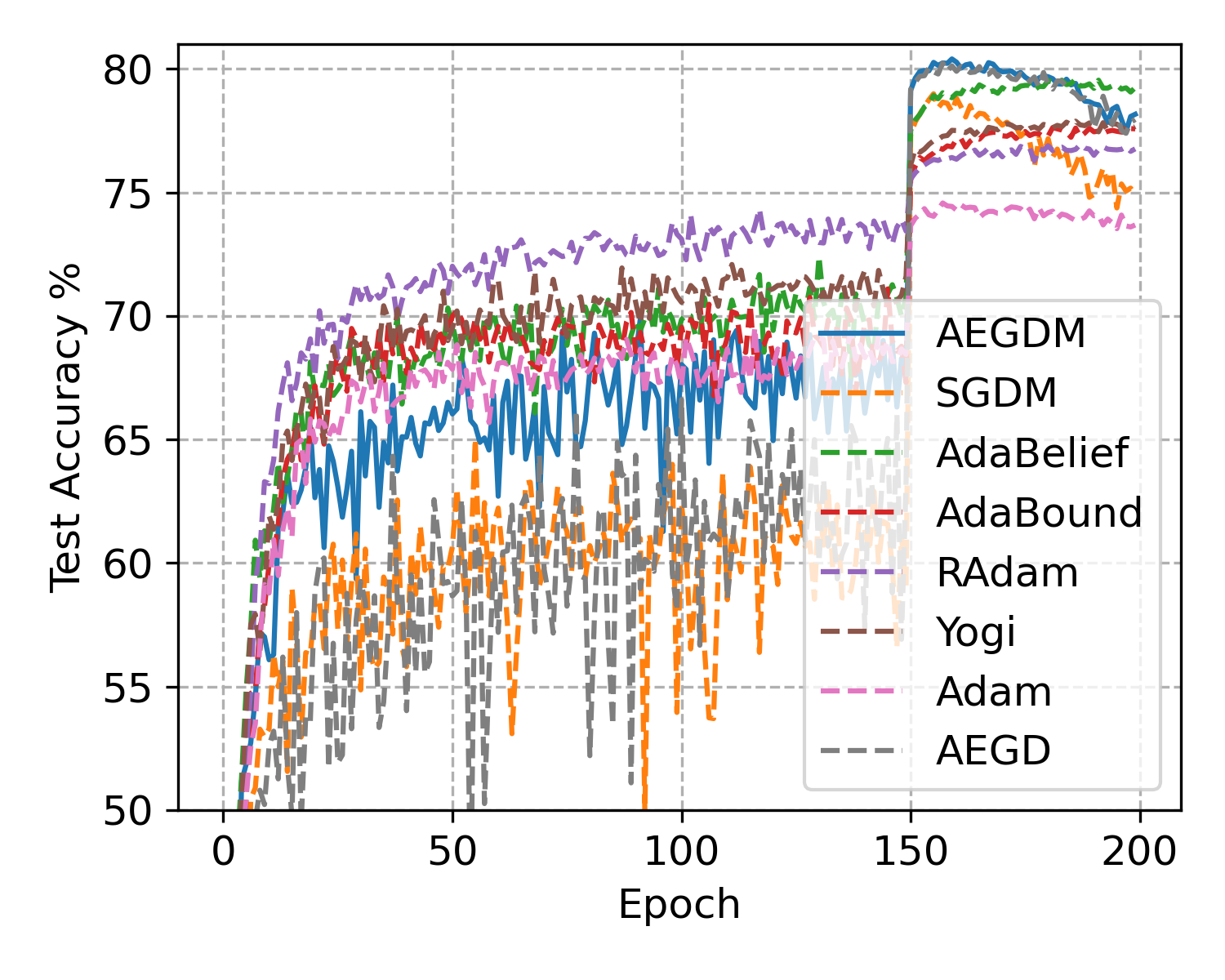
(f) DenseNet-121, test accuracy

Figure 5. Test accuracy for VGG-16, ResNet-34 and DenseNet-121 on CIFAR-100

Appendix H A comparison of some gradient-based methods

How does AEGDM compare with AEGD, SGD, SGDM, Adam and other adaptive methods? We apply a more generic formulation, so that these methods will all take the following form

$$\theta_{t+1}=\theta_{t}-\eta A_{t}^{-1}m_{t+1}.$$ (8.1)

Here $m_{t+1}$ depends on $\{v_{j}\}_{j=0}^{t}$, historical search direction, and $A^{-1}_{t}$ is a diagonal matrix. The diagonal form of $A^{-1}_{t}$ allows for different effective learning rates for different coordinates. The use of inverse $A_{t}^{-1}$ here is to be consistent with the form of the natural gradient method [2], $\theta\leftarrow\theta-\eta A^{-1}\nabla f(\theta)$, in which $A$ is typically a positive definite matrix, playing the role of a metric matrix for certain Riemannian manifold. Table 2 is a comparison in terms of different choices of $A_{t}^{-1}$ and/or $m_{t+1}$.

Table 2. Comparison of some optimization algorithms

	$v_{t}$	$m_{t+1}$	$A^{-1}_{t}$
SGD	$\nabla f_{t}(\theta_{t})$	$v_{t}$	$\mathbb{I}$
SGDM	$\nabla f_{t}(\theta_{t})$	$\sum_{j=0}^{t}\mu^{t-j}v_{j}$	$\mathbb{I}$
RMSprop	$\nabla f_{t}(\theta_{t})$	$v_{t}$	${\rm diag}\Big{[}\Big{(}(1-\beta_{2})\sum_{j=0}^{t}\beta^{t-j}_{2}v_{j}\odot v_{j}\Big{)}^{-\frac{1}{2}}\Big{]}$
ADAM	$\nabla f_{t}(\theta_{t})$	$(1-\beta_{1})\sum_{j=0}^{t}\beta^{t-j}_{1}v_{j}$	${\rm diag}\Big{[}\Big{(}(1-\beta_{2})\sum_{j=0}^{t}\beta^{t-j}_{2}v_{j}\odot v_{j}\Big{)}^{-\frac{1}{2}}\Big{]}$
AEGD	$\frac{\nabla f_{t}(\theta_{t})}{2\sqrt{f_{t}(\theta_{t})+c}}$	$v_{t}$	${\rm diag}\Big{[}r_{0}\odot\Big{(}\prod_{j=0}^{t}(1+2\eta v_{j}\odot v_{j})\Big{)}^{-1}\Big{]}$
AEGDM	$\frac{\nabla f_{t}(\theta_{t})}{2\sqrt{f_{t}(\theta_{t})+c}}$	$\sum_{j=0}^{t}\mu^{t-j}v_{j}$	${\rm diag}\Big{[}r_{0}\odot\Big{(}\prod_{j=0}^{t}(1+2\eta v_{j}\odot v_{j})\Big{)}^{-1}\Big{]}$

Note that in Table 2, the negative power function is understood as an element-wise operation. For the hyper-parameters, $\mu\in(0,1)$ for SGDM and AEGDM; $r_{0}=\sqrt{f_{0}(\theta_{0})+c}{\bf 1}$ for both AEGD and AEGDM; $\beta_{1}\in(0,1)$ and $\beta_{2}\in(0,1)$ for Adam and RMSprop, subject to possible unbiased corrections [17, 41].

References

- [1] Zeyuan Allen-Zhu, Katyusha: The first direct acceleration of stochastic gradient methods, Journal of Machine Learning Research 18 (2018), no. 221, 1–51.
- [2] Shun-ichi Amari, Natural gradient works efficiently in learning, Neural Computation 10 (1998), no. 2, 251–276.
- [3] Leon Bottou, Stochastic gradient descent tricks, neural networks, tricks of the trade, reloaded ed., Lecture Notes in Computer Science (LNCS), vol. 7700, Springer, January 2012.
- [4] Xiangyi Chen, Sijia Liu, Ruoyu Sun, and Mingyi Hong, On the convergence of a class of Adam-type algorithms for non-convex optimization, International Conference on Learning Representations, 2019.
- [5] Aaron Defazio, Francis Bach, and Simon Lacoste-Julien, SAGA: A fast incremental gradient method with support for non-strongly convex composite objectives, Advances in Neural Information Processing Systems, vol. 27, 2014.
- [6] Timothy Dozat, Incorporating Nesterov momentum into Adam, International Conference on Learning Representations, 2016.
- [7] John Duchi, Elad Hazan, and Yoram Singer, Adaptive subgradient methods for online learning and stochastic optimization, Journal of Machine Learning Research 12 (2011), 2121–2159.
- [8] Ian Goodfellow, Yoshua Bengio, and Aaron Courville, Deep learning, MIT Press, 2016, http://www.deeplearningbook.org.
- [9] Elad Hazan, Introduction to online convex optimization, arXiv abs/1909.05207 (2019).
- [10] Kaiming He, Xiangyu Zhang, Shaoqing Ren, and Jian Sun, Deep residual learning for image recognition, 2016 IEEE Conference on Computer Vision and Pattern Recognition (CVPR), 2016, pp. 770–778.
- [11] Gao Huang, Zhuang Liu, Laurens Van Der Maaten, and Kilian Q. Weinberger, Densely connected convolutional networks, 2017 IEEE Conference on Computer Vision and Pattern Recognition (CVPR), 2017, pp. 2261–2269.
- [12] Forrest N. Iandola, M. Moskewicz, Khalid Ashraf, Song Han, W. Dally, and K. Keutzer, Squeezenet: Alexnet-level accuracy with 50x fewer parameters and ¡ 1MB model size, arXiv abs/1602.07360 (2016).
- [13] Stanislaw Jastrzebski, Zachary Kenton, Nicolas Ballas, Asja Fischer, Yoshua Bengio, and Amos J. Storkey, DNN’s sharpest directions along the SGD trajectory, arXiv abs/1807.05031 (2018).
- [14] Chi Jin, Praneeth Netrapalli, and Michael I. Jordan, Accelerated gradient descent escapes saddle points faster than gradient descent, Proceedings of the 31st Conference On Learning Theory, vol. 75, 2018, pp. 1042–1085.
- [15] Rie Johnson and Tong Zhang, Accelerating stochastic gradient descent using predictive variance reduction, Advances in Neural Information Processing Systems, vol. 26, 2013.
- [16] Nitish Shirish Keskar and Richard Socher, Improving generalization performance by switching from Adam to SGD, arXiv abs/1712.07628 (2017).
- [17] Diederik P. Kingma and Jimmy Ba, Adam: A method for stochastic optimization, arXiv abs/1412.6980 (2017).
- [18] Alex Krizhevsky and Geoffrey Hinton, Learning multiple layers of features from tiny images, University of Toronto (2009).
- [19] Y. Lecun, L. Bottou, Y. Bengio, and P. Haffner, Gradient-based learning applied to document recognition, Proceedings of the IEEE 86 (1998), no. 11, 2278–2324.
- [20] Lihua Lei, Cheng Ju, Jianbo Chen, and Michael I Jordan, Non-convex finite-sum optimization via SCSG methods, Advances in Neural Information Processing Systems, vol. 30, 2017.
- [21] Hailiang Liu and Xuping Tian, AEGD: Adaptive gradient decent with energy, arXiv abs/2010.05109 (2020).
- [22] Liyuan Liu, Haoming Jiang, Pengcheng He, Weizhu Chen, Xiaodong Liu, Jianfeng Gao, and Jiawei Han, On the variance of the adaptive learning rate and beyond, International Conference on Learning Representations, 2020.
- [23] Ilya Loshchilov and Frank Hutter, Decoupled weight decay regularization, International Conference on Learning Representations, 2019.
- [24] Liangchen Luo, Yuanhao Xiong, and Yan Liu, Adaptive gradient methods with dynamic bound of learning rate, International Conference on Learning Representations, 2019.
- [25] Yu. E. Nesterov, A method for solving the convex programming problem with convergence rate , Dokl. Akad. Nauk SSSR 269 (1983), no. 3, 543–547. MR 701288
- [26] Yurii Nesterov, Introductory lectures on convex optimization - a basic course, Applied Optimization, 2004.
- [27] Brendan O’donoghue and Emmanuel Candès, Adaptive restart for accelerated gradient schemes, Foundations of Computational Mathematics 15 (2015), no. 3, 715–732.
- [28] Stanley Osher, Bao Wang, Penghang Yin, Xiyang Luo, Farzin Barekat, Minh Pham, and Alex Lin, Laplacian smoothing gradient descent, arXiv abs/1806.06317 (2019).
- [29] B. T. Polyak, Some methods of speeding up the convergence of iterative methods, Ž. Vyčisl. Mat i Mat. Fiz. 4 (1964), 791–803. MR 169403
- [30] B. T. Polyak and A. B. Juditsky, Acceleration of stochastic approximation by averaging, SIAM J. Control Optim. 30 (1992), no. 4, 838–855. MR 1167814
- [31] Ning Qian, On the momentum term in gradient descent learning algorithms, Neural Networks 12 (1999), no. 1, 145–151.
- [32] Sashank Reddi, Satyen Kale, and Sanjiv Kumar, On the convergence of Adam and beyond, International Conference on Learning Representations, 2018.
- [33] Herbert Robbins and Sutton Monro, A stochastic approximation method, Ann. Math. Statistics 22 (1951), 400–407. MR 42668
- [34] Vincent Roulet and Alexandre d'Aspremont, Sharpness, restart and acceleration, Advances in Neural Information Processing Systems (I. Guyon, U. V. Luxburg, S. Bengio, H. Wallach, R. Fergus, S. Vishwanathan, and R. Garnett, eds.), vol. 30, Curran Associates, Inc., 2017.
- [35] David E. Rumelhart, Geoffrey E. Hinton, and Ronald J. Williams, Learning representations by back-propagating errors, p. 696–699, MIT Press, Cambridge, MA, USA, 1988.
- [36] A. Shapiro and Y. Wardi, Convergence analysis of gradient descent stochastic algorithms, J. Optim. Theory Appl. 91 (1996), no. 2, 439–454. MR 1412979
- [37] Jie Shen, Jie Xu, and Jiang Yang, The scalar auxiliary variable (sav) approach for gradient flows, Journal of Computational Physics 353 (2018), 407–416.
- [38] K. Simonyan and Andrew Zisserman, Very deep convolutional networks for large-scale image recognition, arXiv abs/1409.1556 (2015).
- [39] Ilya Sutskever, James Martens, George Dahl, and Geoffrey Hinton, On the importance of initialization and momentum in deep learning, Proceedings of the 30th International Conference on Machine Learning, vol. 28, 2013, pp. 1139–1147.
- [40] Christian Szegedy, Wei Liu, Yangqing Jia, Pierre Sermanet, Scott Reed, Dragomir Anguelov, Dumitru Erhan, Vincent Vanhoucke, and Andrew Rabinovich, Going deeper with convolutions, 2015 IEEE Conference on Computer Vision and Pattern Recognition (CVPR), 2015, pp. 1–9.
- [41] Tijmen Tieleman and Geoffrey Hinton, RMSprop: Divide the gradient by a running average of its recent magnitude, COURSERA: Neural networks for machine learning 4(2) (2012), 26–31.
- [42] Bao Wang, Tan M. Nguyen, Andrea L. Bertozzi, Richard G. Baraniuk, and Stanley J. Osher, Scheduled restart momentum for accelerated stochastic gradient descent, arXiv abs/2002.10583 (2020).
- [43] Ashia C. Wilson, Rebecca Roelofs, Mitchell Stern, Nathan Srebro, and Benjamin Recht, The marginal value of adaptive gradient methods in machine learning, arXiv abs/1705.08292 (2018).
- [44] Xiaofeng Yang, Linear, first and second-order, unconditionally energy stable numerical schemes for the phase field model of homopolymer blends, Journal of Computational Physics 327 (2016), 294–316.
- [45] Matthew D. Zeiler, ADADELTA: An adaptive learning rate method, arXiv abs/1212.5701 (2012).
- [46] Sixin Zhang, Anna E Choromanska, and Yann LeCun, Deep learning with elastic averaging SGD, Advances in Neural Information Processing Systems, vol. 28, 2015.
- [47] Jia Zhao, Qi Wang, and Xiaofeng Yang, Numerical approximations for a phase field dendritic crystal growth model based on the invariant energy quadratization approach, International Journal for Numerical Methods in Engineering 110 (2017), 279–300.
- [48] Martin Zinkevich, Online convex programming and generalized infinitesimal gradient ascent, Proceedings of the Twentieth International Conference on International Conference on Machine Learning, ICML, 2003, p. 928–935.