Visual Prompt Tuning

Abstract

The current modus operandi in adapting pre-trained models involves updating all the backbone parameters, i.e., full fine-tuning. This paper introduces Visual Prompt Tuning (VPT) as an efficient and effective alternative to full fine-tuning for large-scale Transformer models in vision. Taking inspiration from recent advances in efficiently tuning large language models, VPT introduces only a small amount (less than 1% of model parameters) of trainable parameters in the input space while keeping the model backbone frozen. Via extensive experiments on a wide variety of downstream recognition tasks, we show that VPT achieves significant performance gains compared to other parameter efficient tuning protocols. Most importantly, VPT even outperforms full fine-tuning in many cases across model capacities and training data scales, while reducing per-task storage cost. Code is available at github.com/kmnp/vpt.

1 Introduction

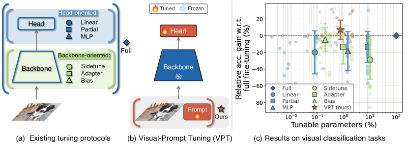
Figure 1: Visual-Prompt Tuning (VPT) vs. other transfer learning methods. (a) Current transfer learning protocols are grouped based on the tuning scope: Full fine-tuning, Head-oriented, and Backbone-oriented approaches. (b) VPT instead adds extra parameters in the input space. (c) Performance of different methods on a wide range of downstream classification tasks adapting a pre-trained ViT-B backbone, with mean and standard deviation annotated. VPT outperforms Full fine-tuning 20 out of 24 cases while using less than 1$\%$ of all model parameters

For a variety of recognition applications, the most accurate results are now obtained by adapting large foundation models pre-trained on massive curated or raw data, a finding that mirrors developments in natural language processing (NLP) [6]. At first glance,this is a success story: one can make rapid progress on multiple recognition problems simply by leveraging the latest and greatest foundation model. In practice, however, adapting these large models to downstream tasks presents its own challenges. The most obvious (and often the most effective) adaptation strategy is full fine-tuning of the pre-trained model on the task at hand, end-to-end. However, this strategy requires one to store and deploy a separate copy of the backbone parameters for every single task. This is an expensive and often infeasible proposition, especially for modern Transformer-based architectures, which are significantly larger than their convolutional neural networks (ConvNet) counterparts, e.g., ViT-Huge [19] (632M parameters) vs. ResNet-50 [31] (25M parameters). We therefore ask, what is the best way to adapt large pre-trained Transformers to downstream tasks in terms of effectiveness and efficiency?

One straightforward approach is to turn to other strategies that we have perfected for adapting ConvNets to new tasks, as in Fig. 1(a). A popular approach is to fine-tune only a subset of the parameters, such as the classifier head [56, 36, 11] or the bias terms [8]. Prior research has also looked at adding additional residual blocks (or adapters) to the backbone [68, 87]. One could implement similar strategies for Transformers. However, in general these strategies under-perform full fine-tuning in accuracy.

We explore a different route in this paper. Instead of altering or fine-tuning the pre-trained Transformer itself, we modify the input to the Transformer. Drawing inspiration from the recent advances on Prompting in NLP [50, 48, 45, 51], we propose a new simple and efficient method to adapt transformer models for downstream vision tasks (Fig. 1(b)), namely Visual-Prompt Tuning (VPT). Our method only introduces a small amount of task-specific learnable parameters into the input space while freezing the entire pre-trained Transformer backbone during downstream training. In practice, these additional parameters are simply prepended into the input sequence of each Transformer layer and learned together with a linear head during fine-tuning.

On 24 downstream recognition tasks spanning different domains using a pre-trained ViT backbone, VPT beats all other transfer learning baselines, even surpassing full fine-tuning in 20 cases, while maintaining the advantage of storing remarkably fewer parameters (less than 1% of backbone parameters) for each individual task (Fig. 1(c)). This result demonstrates the distinctive strength of visual prompting: whereas in NLP, prompt tuning is only able to match full fine-tuning performance under certain circumstances [45]. VPT is especially effective in the low-data regime, and maintains its advantage across data scales. Finally, VPT is competitive for a range of Transformer scales and designs (ViT-Base/Large/Huge, Swin). Put together, our results suggest that VPT is one of the most effective ways of adapting ever-growing vision backbones.

2 Related Work

Transformer models [73] have gained huge success in NLP [17, 66, 7]. The triumph of the Transformer architecture also extends to various computer vision tasks, including image classification [19, 52], object detection [9, 49], semantic and panoptic segmentation [71, 89, 78], video understanding [25, 79, 21] and few-shot learning [18], surpassing previous state-of-the-art approaches. Transformers are also being widely used in recent self-supervised pre-training methods [11, 30, 3]. Given their superior performance and much larger scale compared to ConvNets, how to efficiently adapt Transformers to different vision tasks remains an important open problem. Our proposed VPT provides a promising path forward.

Transfer learning has been extensively studied for vision tasks in the context of ConvNets [92] and many techniques have been introduced including side tuning [87], residual adapter [67], bias tuning [8], etc. Relatively little attention has been paid to vision Transformers adaptation and how well these aforementioned methods perform on this brand new type of architecture remains unknown. On the other hand, given the dominance of large-scale pre-trained Transformer-based Language Models (LM) [17, 66, 7], many approaches [29, 28, 35] have been proposed to efficiently fine-tune LM for different downstream NLP tasks [77, 76]. Among them, we focus on the following two representative methods in our experiments for benchmarking purposes: Adapters [64] and BitFit [5].

Adapters [34] insert extra lightweight modules inside each Transformer layer. One adapter module generally consists of a linear down-projection, followed by a nonlinear activation function, and a linear up-projection, together with a residual connection [63, 64]. Instead of inserting new modules, [8] proposed to update the bias term and freeze the rest of backbone parameters when fine-tuning ConvNets. BitFit [3] applied this technique to Transformers and verified its effectiveness on LM tuning. Our study demonstrates that VPT, in general, provides improved performance in adapting Transformer models for vision tasks, relative to the aforementioned two well-established methods in NLP.

Prompting [50] originally refers to prepending language instruction to the input text so that a pre-trained LM can “understand” the task. With manually chosen prompts, GPT-3 shows strong generalization to downstream transfer learning tasks even in the few-shot or zero-shot settings [7]. In addition to the follow-up works on how to construct better prompting texts [70, 37], recent works propose to treat the prompts as task-specific continuous vectors and directly optimize them via gradients during fine-tuning, namely Prompt Tuning [48, 45, 51]. Compared to full fine-tuning, it achieves comparable performance but with 1000$\times$ less parameter storage. Although prompting has also been applied to vision-language models recently [65, 91, 39, 84, 22], prompting is still limited to the input of text encoders. Due to the disparity between vision and language modalities, in this paper we ask: can the same method can be applied successfully to image encoders? We are the first work (see related concurrent works [69, 80, 14, 2]) to tackle this question and investigate the generality and feasibility of visual prompting via extensive experiments spanning multiple kinds of recognition tasks across multiple domains and backbone architectures.

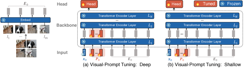
Figure 2: Overview of our proposed Visual-Prompt Tuning. We explore two variants: (a) prepend a set of learnable parameters to each Transformer encoder layer’s input (VPT-deep); (b) only insert the prompt parameters to the first layer’s input (VPT-shallow). During training on downstream tasks, only the parameters of prompts and linear head are updated while the whole Transformer encoder is frozen.

3 Approach

We propose Visual-Prompt Tuning (VPT) for adapting large pre-trained vision Transformer models. VPT injects a small number of learnable parameters into Transformer’s input space and keeps the backbone frozen during the downstream training stage. The overall framework is presented in Fig. 2. We first define the notations in Sec. 3.1, then describe VPT formally in Sec. 3.2.

3.1 Preliminaries

For a plain Vision Transformer (ViT) [19] with $N$ layers, an input image is divided into $m$ fixed-sized patches $\{I_{j}\in\mathbb{R}^{3\times h\times w}\mid j\in\mathbb{N},1\leq j\leq m\}$. $h,w$ are the height and width of the image patches. Each patch is then first embedded into $d$-dimensional latent space with positional encoding:

$$\mathbf{e}_{0}^{j}=\texttt{Embed}(I_{j}) \mathbf{e}_{0}^{j}\in\mathbb{R}^{d},j=1,2,\ldots m\;\;.$$ (1)

We denote the collection of image patch embeddings, $\mathbf{E}_{i}=\{\mathbf{e}_{i}^{j}\in\mathbb{R}^{d}\mid j\in\mathbb{N},1\leq j\leq m\}$, as inputs to the ($i$+$1$)-th Transformer layer ($L_{i+1}$). Together with an extra learnable classification token ([CLS]), the whole ViT is formulated as:

$$[\mathbf{x}_{i},\mathbf{E}_{i}] =L_{i}([\mathbf{x}_{i-1},\mathbf{E}_{i-1}]) i=1,2,\ldots,N$$ (2)

$$\mathbf{y} =\texttt{Head}(\mathbf{x}_{N})\;\;,$$ (3)

where $\mathbf{x}_{i}\in\mathbb{R}^{d}$ denote [CLS]’s embedding at $L_{i+1}$’s input space. $[\cdot,\cdot]$ indicates stacking and concatenation on the sequence length dimension, i.e., $[\mathbf{x}_{i},\mathbf{E}_{i}]\in\mathbb{R}^{(1+m)\times d}$. Each layer $L_{i}$ consists of Multiheaded Self-Attention (MSA) and Feed-Forward Networks (FFN) together with LayerNorm [1] and residual connections [31]. A neural classification head is used to map the final layer’s [CLS] embedding, $\mathbf{x}_{N}$, into a predicted class probability distribution $\mathbf{y}$.

3.2 Visual-Prompt Tuning (VPT)

Given a pre-trained Transformer model, we introduce a set of $p$ continuous embeddings of dimension $d$, i.e., prompts, in the input space after the Embed layer. Only the task-specific prompts are being updated during fine-tuning, while the Transformer backbone is kept frozen. Depending on the number of Transformer layers involved, our approach has two variants, VPT-shallow and VPT-deep, as shown in Fig. 2.

3.2.1 VPT-Shallow.

Prompts are inserted into the first Transformer layer $L_{1}$ only. Each prompt token is a learnable $d$-dimensional vector. A collection of $p$ prompts is denoted as $\mathbf{P}=\{\mathbf{p}^{k}\in\mathbb{R}^{d}\mid k\in\mathbb{N},1\leq k\leq p\}$, the shallow-prompted ViT is:

$$[\mathbf{x}_{1},\mathbf{Z}_{1},\mathbf{E}_{1}] ={\color[rgb]{0.12109375,0.46875,0.70703125}L_{1}}([{\color[rgb]{0.12109375,0.46875,0.70703125}\mathbf{x}_{0}},{\color[rgb]{0.83203125,0.359375,0.26171875}\mathbf{P}},\mathbf{E}_{0}])$$ (4)

$$[\mathbf{x}_{i},\mathbf{Z}_{i},\mathbf{E}_{i}] ={\color[rgb]{0.12109375,0.46875,0.70703125}L_{i}}([\mathbf{x}_{i-1},\mathbf{Z}_{i-1},\mathbf{E}_{i-1}]) i=2,3,\ldots,N$$ (5)

$$\mathbf{y} ={\color[rgb]{0.83203125,0.359375,0.26171875}\texttt{Head}}(\mathbf{x}_{N})\;\;,$$ (6)

where $\mathbf{Z}_{i}\in\mathbb{R}^{p\times d}$ represents the features computed by the $i$-th Transformer layer, and $[\mathbf{x}_{i},\mathbf{Z}_{i},\mathbf{E}_{i}]\in\mathbb{R}^{(1+p+m)\times d}$. The colors $\bullet$ and $\bullet$ indicate learnable and frozen parameters, respectively. Notably for ViT, $\mathbf{x}_{N}$ is invariant to the location of prompts since they are inserted after positional encoding, e.g., $[\mathbf{x}_{0},\mathbf{P},\mathbf{E}_{0}]$ and $[\mathbf{x}_{0},\mathbf{E}_{0},\mathbf{P}]$ are mathematically equivalent. This also applies to VPT-Deep.

3.2.2 VPT-Deep.

Prompts are introduced at every Transformer layer’s input space. For ($i$+$1$)-th Layer $L_{i+1}$, we denote the collection of input learnable prompts as $\mathbf{P}_{i}=\{\mathbf{p}_{i}^{k}\in\mathbb{R}^{d}\mid k\in\mathbb{N},1\leq k\leq m\}$. The deep-prompted ViT is formulated as:

$$[\mathbf{x}_{i},\underline{\hskip 8.5359pt},\mathbf{E}_{i}] ={\color[rgb]{0.12109375,0.46875,0.70703125}L_{i}}([\mathbf{x}_{i-1},{\color[rgb]{0.83203125,0.359375,0.26171875}\mathbf{P}_{i-1}},\mathbf{E}_{i-1}]) i=1,2,\ldots,N$$ (7)

$$\mathbf{y} ={\color[rgb]{0.83203125,0.359375,0.26171875}\texttt{Head}}(\mathbf{x}_{N})\;\;.$$ (8)

3.2.3 Storing Visual Prompts.

VPT is beneficial in presence of multiple downstream tasks. We only need to store the learned prompts and classification head for each task and re-use the original copy of the pre-trained Transformer model, significantly reducing the storage cost. For instance, given a ViT-Base with 86 million (M) parameters and $d=768$, 50 shallow prompts and deep prompts yield additional $p\times d=50\times 768=0.038$M, and $N\times p\times d=0.46$M parameters, amounting to only 0.04$\%$ and 0.53$\%$ of all ViT-Base parameters, respectively.

4 Experiments

We evaluate VPT for a wide range of downstream recognition tasks with pre-trained Transformer backbones across scales. We first describe our experimental setup in Sec. 4.1, including the pre-trained backbone and downstream tasks, and a brief introduction of alternative transfer learning methods. Then we demonstrate the effectiveness and practical utility of our method in Sec. 4.2. We also systematically study how different design choices would affect performance (Sec. 4.3), which leads to an improved understanding of our approach.

4.1 Experiment Setup

Pre-trained Backbones. We experiment with two Transformer architectures in vision, Vision Transformers (ViT) [19] and Swin Transformers (Swin [52]). All backbones in this section are pre-trained on ImageNet-21k [16]. We follow the original configurations, e.g., number of image patches divided, existence of [CLS], etc. More details are included in Appendix 0.A.

Baselines. We compare both variants of VPT with other commonly used fine-tuning protocols:

1. Full: fully update all backbone and classification head parameters.

2. Methods that focus on the classification head. They treat the pre-trained backbone as a feature extractor, whose weights are fixed during tuning:

   • Linear: only use a linear layer as the classification head.

   • Partial-$k$: fine-tune the last $k$ layers of backbone while freezing the others, as adopted in [85, 88, 60, 30]. It redefines the boundary of backbone and classification head.

   • Mlp-$k$: utilize a multilayer perceptron (MLP) with $k$ layers, instead of a linear layer, as classification head.

3. Methods that update a subset backbone parameters or add new trainable parameters to backbone during fine-tuning:

   • Sidetune [87]: train a “side” network and linear interpolate between pre-trained features and side-tuned features before being fed into the head.

   • Bias [8, 5]: fine-tune only the bias terms of a pre-trained backbone.

   • Adapter [34, 63, 64]: insert new MLP modules with residual connection inside Transformer layers.

   Downstream Tasks. We experiment on the following two collections of datasets:

   FGVC consists of 5 benchmarked Fine-Grained Visual Classification tasks including CUB-200-2011 [75], NABirds [72], Oxford Flowers [59], Stanford Dogs [41] and Stanford Cars [23]. If a certain dataset only has train and test sets publicly available, we randomly split the training set into train (90%) and val (10%), and rely on val to select hyperparameters.

   VTAB-1k [86] is a collection of 19 diverse visual classification tasks, which are organized into three groups: Natural - tasks that contain natural images captured using standard cameras; Specialized - tasks that contain images captured via specialized equipment, such as medical and satellite imagery; and Structured - tasks that require geometric comprehension like object counting. Each task of VTAB contains 1000 training examples. Following [86], we use the provided 800-200 split of the train set to determine hyperparameters and run the final evaluation using the full training data. We report the average accuracy score on test set within three runs.

   We report the average accuracy on the FGVC datasets, and the average accuracy on each of the three groups in VTAB. The individual results on each task are in Appendix 0.D, as are image examples of these aforementioned tasks.

   Table 1: ViT-B/16 pre-trained on supervised ImageNet-21k. For each method and each downstream task group, we report the average test accuracy score and number of wins in ($\cdot$) compared to Full. “Total params” denotes total parameters needed for all 24 downstream tasks. “Scope” denotes the tuning scope of each method. “Extra params” denotes the presence of additional parameters besides the pre-trained backbone and linear head. Best results among all methods except Full are bolded. VPT outshines the full fine-tuning 20 out of 24 cases with significantly less trainable parameters

   	ViT-B/16	Total	Scope		Extra	FGVC	VTAB-1k
   	(85.8M)	params	Input	Backbone	params		Natural	Specialized	Structured
   	Total # of tasks					5	7	4	8
   (a)	Full	24.02$\times$		✓		88.54	75.88	83.36	47.64
   (b)	Linear	1.02$\times$				79.32 (0)	68.93 (1)	77.16 (1)	26.84 (0)
   	Partial-1	3.00$\times$				82.63 (0)	69.44 (2)	78.53 (0)	34.17 (0)
   	Mlp-3	1.35$\times$			✓	79.80 (0)	67.80 (2)	72.83 (0)	30.62 (0)
   (c)	Sidetune	3.69$\times$		✓	✓	78.35 (0)	58.21 (0)	68.12 (0)	23.41 (0)
   	Bias	1.05$\times$		✓		88.41 (3)	73.30 (3)	78.25 (0)	44.09 (2)
   	Adapter	1.23$\times$		✓	✓	85.66 (2)	70.39 (4)	77.11 (0)	33.43 (0)
   (ours)	VPT-shallow	1.04$\times$	✓		✓	84.62 (1)	76.81 (4)	79.66 (0)	46.98 (4)
   	VPT-deep	1.18$\times$				89.11 (4)	78.48 (6)	82.43 (2)	54.98 (8)

   4.2 Main Results

   Tab. 1 presents the results of fine-tuning a pre-trained ViT-B/16 on averaged across 4 diverse downstream task groups, comparing VPT to the other 7 tuning protocols. We can see that:

   1. VPT-Deep outperforms Full (Tab. 1(a)) on 3 out of the 4 problem classes (20 out of 24 tasks), while using significantly fewer total model parameters (1.18$\times$ vs. 24.02$\times$). Thus, even if storage is not a concern, VPT is a promising approach for adapting larger Transformers in vision. Note that this result is in contrast to comparable studies in NLP, where prompt tuning matches, but does not exceed full fine-tuning [45].

   2. VPT-Deep outperforms all the other parameter-efficient tuning protocols (Tab. 1(b,c)) across all task groups, indicating that VPT-deep is the best fine-tuning strategy in storage-constrained environments.

   3. Although sub-optimal than VPT-deep, VPT-shallow still offers non-trivial performance gain than head-oriented tuning methods in Tab. 1(b), indicating that VPT-shallow is a worthwhile choice in deploying multi-task fine-tuned models if the storage constraint is severe.

   

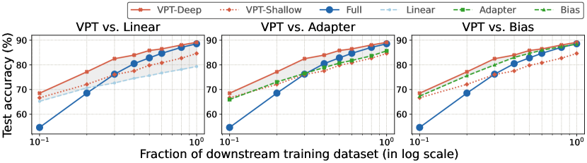
   Figure 3: Performance comparison on different downstream data scales, averaged across 5 FGVC tasks. VPT-deep is compared with Linear (left), Adapter (middle) and Bias (right). Highlighted region shows the accuracy difference between VPT-deep and the compared method. Results of VPT-shallow are Full presented in all plots for easy reference. The size of markers are proportional to the percentage of tunable parameters in log scale

   4.2.1 VPT on different downstream data size.

   We look at the impact of training data size on accuracy in the FGVC tasks (VTAB has only 1k training examples). We vary the training data between 10% and 80% and compare all methods. The same pre-trained ViT-B is used for downstream training. Task-averaged results for each method on different training data scales are presented in Fig. 3.

   Fig. 3 shows that VPT-deep outperforms all the other baselines across data scales. Digging deeper, methods that use less trainable parameters, i.e., VPT, Linear, Adapter, Bias, dominate over Full in the low-data regimes. This trend, however, is reversed when more training data is available for Linear and Adapter. In contrast, VPT-deep still consistently outperforms Fullacross training data sizes. Although Bias offers similar advantages, it still marginally under-performs VPT-deep across the board (Fig. 3 right).

   

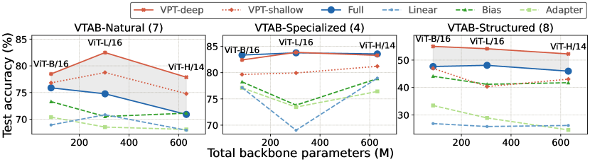
   Figure 4: VPT vs. Full across model scales (ViT-B, ViT-L and ViT-H), for 3 VTAB task groups. Highlighted region shows the accuracy difference between VPT-deep and the full fine-tuning (Full). The size of markers are proportional to the percentage of trainable parameters in log scale

   4.2.2 VPT on different backbone scales.

   Fig. 4 shows VTAB-1k performance under 3 different backbone scales: ViT-Base/Large/Huge. VPT-deep is significantly better than Linear and VPT-shallow across all 3 backbone choices and 3 subgroups of VTAB-1k. More importantly, the advantages of VPT-deep over Full indeed still hold as the model scale increases, i.e., VPT-deep significantly outperforms Full on Natural and Structured groups, while offering nearly equivalent performance on Specialized.

   Table 2: Different Transformer architecture: Swin-B pre-trained on supervised ImageNet-21k as backbone. For each method and each downstream task group, we report the average test accuracy score and number of wins in ($\cdot$) compared to Full. The column “Total params” denotes total parameters needed for all 19 downstream tasks. Best results among all methods except Full are bolded

   	Swin-B	Total	VTAB-1k
   	(86.7M)	params	Natural	Specialized	Structured
   	Total # of tasks		7	4	8
   (a)	Full	19.01$\times$	79.10	86.21	59.65
   (b)	Linear	1.01$\times$	73.52 (5)	80.77 (0)	33.52 (0)
   	Mlp-3	1.47$\times$	73.56 (5)	75.21 (0)	35.69 (0)
   	Partial	3.77$\times$	73.11 (4)	81.70 (0)	34.96 (0)
   (c)	Bias	1.06$\times$	74.19 (2)	80.14 (0)	42.42 (0)
   (ours)	VPT-shallow	1.01$\times$	79.85 (6)	82.45 (0)	37.75 (0)
   	VPT-deep	1.05$\times$	76.78 (6)	84.53 (0)	53.35 (0)

   4.2.3 VPT on hierarchical Transformers.

   We extend VPT to Swin [52], which employs MSA within local shifted windows and merges patch embeddings at deeper layers. For simplicity and without loss of generality, we implement VPT in the most straightforward manner: the prompts are attended within the local windows, but are ignored during patch merging stages. The experiments are conducted on the ImageNet-21k supervised pre-trained Swin-Base. VPT continues to outperform other parameter-efficient fine-tuning methods (b, c) for all three subgroups of VTAB Tab. 2, though in this case Full yields the highest accuracy scores overall (at a heavy cost in total parameters).

   It is surprising that the advantage of VPT-deep over VPT-shallow diminishes for Natural: VPT-shallow yields slightly better accuracy scores than full fine-tuning.

   4.3 Ablation on Model Design Variants

   We ablate different model design choices on the supervised ImageNet-21k pre-trained ViT-Base and evaluate them on VTAB, with same setup in Tab. 1. See more in Appendix 0.B.

   

   

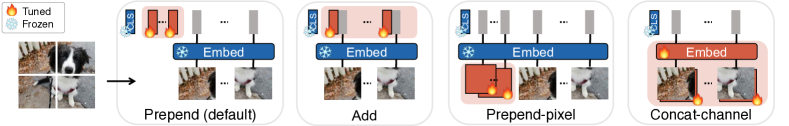
   Figure 5: Ablation on prompt location. We illustrate different location choices at top, and present the results at bottom. For easy comparison, two blue dashed lines represent the performance of the default VPT-deep and VPT-shallow respectively

   4.3.1 Prompt Location.

   An important distinction between VPT and other methods is the extra learnable parameters introduced as inputs for the Transformer layers. Fig. 5 ablates different choices on how and where to insert prompts in the input space, and how they would affect the final performance.

   Prepend or Add? Instead of prepending prompts to the sequence of the image patches embeddings $\mathbf{E}_{i}$ as described in Sec. 3.2, another option is to directly add prompts element-wise to those embeddings, keeping the Transformer’s input sequence length the same as before. Though this variant is competitive to Full in some cases (e.g., VTAB-Natural), its performance generally falls behind with the default Prepend in both deep and shallow settings. More discussion on this phenomenon is in Sec. 0.B.0.1.

   Latent or pixel space? Instead of inserting the prompts as latent vectors for the first Transformer layer, one could introduce prompts in the pixel level before the Embed layer in Eq. 1, i.e., Prepend-pixel and Concat-channel. Fig. 5 shows that the adaption performance decreases for these two variants. For example, the accuracy score of prepending shallow prompts before the projection layer (Prepend-pixel) drops 6.9$\%$, compared to the default prepending in the embedding space (Prepend) on VTAB-Natural. The performance further deteriorates (even as large as 30 accuracy scores drop on VTAB-Natural) if we instead concatenate a new channel to the input image (Concat-channel). These observations suggest that it’s easier for prompts to learn condensed task-dependent signals in the latent input space of Transformers.

   

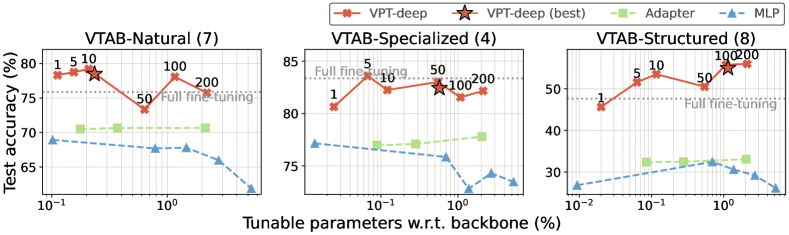
   Figure 6: Ablation on prompt length. We vary the number of prompts for VPT-deep and show the averaged results for each VTAB subgroup. The averaged best VPT-deep results for each task is also shown for easy reference

   4.3.2 Prompt Length.

   This is the only additional hyper-parameter needed to tune for VPT compared to full fine-tuning. For easy reference, we also ablate two other baselines on their individual additional hyper-parameters, i.e., number of layers for Mlp and reduction rate for Adapter. As shown in Fig. 6, the optimal prompt length varies across tasks. Notably, even with as few as only one prompt, VPT-deep still significantly outperforms the other 2 baselines, and remains competitive or even better compared to full fine-tuning on VTAB-Structured and Natural.

   

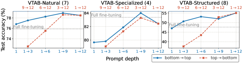
   Figure 7: Ablation on prompt depth. We select the best prompt length for each variant with val sets. $i\rightarrow j$ indicates the Transformer layer indices that prompts are inserted into. The 1-st layer refers to the one closest to input. ViT-B has 12 layers in total

   4.3.3 Prompt Depth.

   Fig. 7 ablates which and how many layers to insert prompts. Each variant reports the best prompt length selected with val set. VPT’s performance is positively correlated with the prompt depth in general. Yet the accuracy drops if we insert prompts from top to bottom, suggesting that prompts at earlier Transformer layers matter more than those at later layers.

   

   

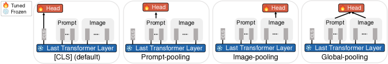
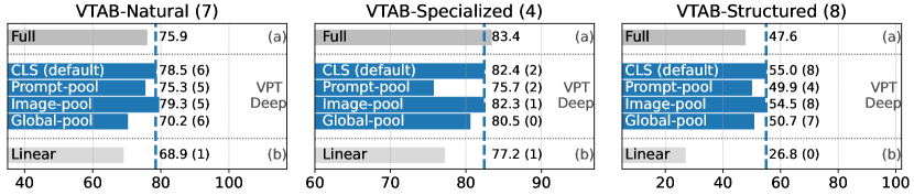
   Figure 8: Ablation on final output. Illustration of different strategies is included at top, and results of those are presented at the bottom section. For easy comparison, the blue dashed line represents the performance of default VPT-deep

   4.3.4 Final Output.

   Following the original configuration of ViT, we use the final embedding of [CLS], i.e., $\mathbf{x}_{N}$, as the classification head input, which is also the default setting in our ViT experiments. As shown in Fig. 8, if we use the average pooling on image patch output embeddings $\mathbf{E}_{N}$ as final output (Image-pool), the results essentially remain the same (e.g., 82.4 vs. 82.3 for VTAB-Specialized). However, if the pooling involves final prompt outputs $\mathbf{Z}_{N}$ (Prompt-pool and Global-pool), the accuracy could drop as large as 8 points.

   

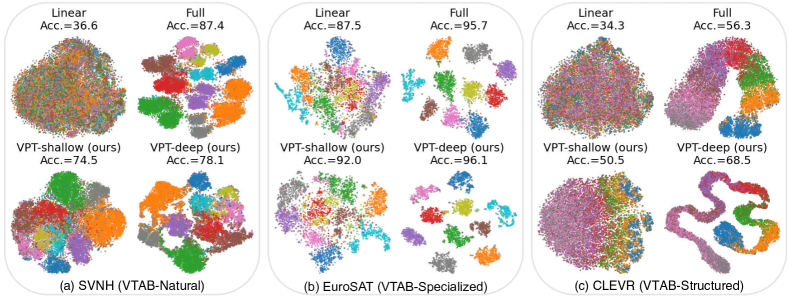
   Figure 9: t-SNE visualizations of the final [CLS] embedding $\mathbf{x}_{N}$ of 3 VTAB tasks from the test set, from Tab. 1. VPT could produce linearly separable features without updating backbone parameters

   5 Analysis and Discussion

   5.0.1 Visualization.

   Fig. 9 shows t-SNE [55] visualizations of $\mathbf{x_{N}}$, i.e., embeddings of [CLS] after the last Transformer layer and before the classification head, for 3 tasks in VTAB (SVNH [58], EuroSAT [32], Clevr/count [38]), one for each subgroup. All plots show that VPT-deep enables linearly separable representations while using less parameters than Full. We also observe that extra tunable parameters for every Transformer layer (VPT-deep) improve the performance, compared to VPT-shallow, which only inserts prompts for the first layer’s input. Interestingly on Clevr/count (Fig. 9(c)), VPT-deep and Full recover the underlying manifold structure of the task (counting objects in images vs. street number or landscape recognition), unlike VPT-shallow and Linear.

   Table 3: Semantic Segmentation: ADE20k [90] validation results with SETR [89] on ViT-L. The best mIoU scores among all methods but Full are bolded. Results of fully fine-tuning a ResNet-101 [10] are included. SS/MS: single/multi-scale inference

   Backbone	ViT-L/16					ResNet-101
   Method	Full [89]	Head Only	Bias	VPT-deep	VPT+Bias	Full [10]
   mIoU-SS	48.31	35.12	43.40	42.11	44.04	45.47
   mIoU-MS	50.07	37.46	45.33	44.06	45.63	46.27
   Tunable params (M)	318.31	13.18	13.46	13.43	15.79	63.0

   5.0.2 Apply VPT to more vision tasks.

   We explore the feasibility of VPT beyond visual classification, by evaluating ADE20K [90] semantic segmentation task with a Transformer model, SETR-PUP [89]. It adds a standard ConvNet head to the ViT backbone to perform segmentation. The de-facto approach is still fully fine-tuning the pre-trained backbone together with the ConvNet head (Full). We include two more protocols for comparison: only update the head layers (Head Only), update head layers and bias vectors in the backbone (Bias). In Tab. 3, we report val mIoU results with and without multi-scale inference. Though parameter-efficient protocols could not compete with Full, VPT is still comparable with Bias. Notably, VPT offers competitive results to a fully fine-tuned state-of-the-art ConvNet model (DeepLab v3+ [10]), while tuning significantly less parameters (15M vs. 64M, respectively).

   Table 4: Different pre-trained objectives: MAE [30] and MoCo v3 [11] with a ViT-B backbone. For each method and each downstream task group, we report the average test accuracy score and number of wins in ($\cdot$) compared to Full. “Total params” denotes total parameters needed for all 24 downstream tasks. Best results among all methods except Full are bolded

   		MAE				MoCo v3
   	ViT-B/16	Total	VTAB-1k			Total	VTAB-1k
   	(85.8M)	params	Natural	Specialized	Structured	params	Natural	Specialized	Structured
   	Total # of tasks		7	4	8		7	4	8
   (a)	Full	19.01$\times$	59.29	79.68	53.82	19.01$\times$	71.95	84.72	51.98
   (b)	Linear	1.01$\times$	18.87 (0)	53.72 (0)	23.70 (0)	1.01$\times$	67.46 (4)	81.08 (0)	30.33 (0)
   	Partial-1	2.58$\times$	58.44 (5)	78.28 (1)	47.64 (1)	2.58$\times$	72.31 (5)	84.58 (2)	47.89 (1)
   (c)	Bias	1.03$\times$	54.55 (1)	75.68 (1)	47.70 (0)	1.03$\times$	72.89 (3)	81.14 (0)	53.43 (4)
   	Adapter	1.17$\times$	54.90 (3)	75.19 (1)	38.98 (0)	1.22$\times$	74.19 (4)	82.66 (1)	47.69 (2)
   (ours)	VPT-shallow	1.01$\times$	39.96 (1)	69.65 (0)	27.50 (0)	1.01$\times$	67.34 (3)	82.26 (0)	37.55 (0)
   	VPT-deep	1.04$\times$	36.02 (0)	60.61 (1)	26.57 (0)	1.01$\times$	70.27 (4)	83.04 (0)	42.38 (0)

   5.0.3 Apply VPT to more pre-training methods.

   In addition to the backbones pre-trained with labeled data, we experiment with two self-supervised objectives: MAE [30] and MoCo v3 [11]. Tab. 4 reports the results on VTAB-1k with ViT-B. We observe that both variants of VPT surpass Linear, yet the comparisons among other techniques are less conclusive. For MAE, other parameter-efficient methods, e.g., Partial-1, outperform both VPT and Linear. In the case of MoCo v3, VPT no longer holds the best performance, though it is still competitive with the others. This suggests that these two self-supervised ViTs are fundamentally different from the supervised ones in previous sections. Exactly why and how these differences arise remain open questions.

   Table 5: Apply VPT to ConvNets: ResNet-50 and ConvNeXt-Base. For each method and each downstream task group, we report the average test accuracy score and number of wins in ($\cdot$) compared to Full. “Total params” denotes total parameters needed for all 19 downstream tasks. Best results among all methods except Full are bolded

   		ConvNeXt-Base (87.6M)				ResNet-50 (23.5M)
   		Total	VTAB-1k			Total	VTAB-1k
   		params	Natural	Specialized	Structured	params	Natural	Specialized	Structured
   	Total # of tasks		7	4	8		7	4	8
   (a)	Full	19.01$\times$	77.97	83.71	60.41	19.08$\times$	59.72	76.66	54.08
   (b)	Linear	1.01$\times$	74.48 (5)	81.50 (0)	34.76 (1)	1.08$\times$	63.75 (6)	77.60 (3)	30.96 (0)
   	Partial-1	2.84$\times$	73.76 (4)	81.64 (0)	39.55 (0)	4.69$\times$	64.34 (6)	78.64 (2)	45.78 (1)
   	Mlp-3	1.47$\times$	73.78 (5)	81.36 (1)	35.68 (1)	7.87$\times$	61.79 (6)	70.77 (1)	33.97 (0)
   (c)	Bias	1.04$\times$	69.07 (2)	72.81 (0)	25.29 (0)	1.10$\times$	63.51 (6)	77.22 (2)	33.39 (0)
   (ours)	Visual-Prompt Tuning	1.02$\times$	78.48 (6)	83.00 (1)	44.64 (1)	1.09$\times$	66.25 (6)	77.32 (2)	37.52 (0)

   5.0.4 Apply VPT to ConvNets.

   We examine the idea of adding trainable parameters in the input space of ConvNets: padding both height and width by $p$ learnable prompt pixels for the input image. Though this operation seems unconventional, we implement VPT this way given there is no obvious solution to add location-invariant prompts similar to the Transformer counterparts. In fact this approach has been explored before in the adversarial attack literature [20]. The value of $p$ in our experiment is 2 orders of magnitude smaller than previous work: e.g., 5 vs. 263. Most importantly, we cast this idea in the lens of transfer learning. See Sec. 0.C.0.1 for more discussion.

   Tab. 5 presents the results for ConvNeXt-B [53] (pre-trained on ImageNet-21k) and ResNet-50 [31] (pre-trained on ImageNet-1k), respectively. VPT works well in a larger ConvNet backbone, ConvNeXt-B, offering accuracy gains over other sparse tuning protocols (b, c), and outperforming Full on 8 out of 19 cases. The advantages of VPT, however, diminish with smaller ConvNet (ResNet-50), as there is no clear winner for all 19 VTAB-1k tasks.

   6 Conclusion

   We present Visual Prompt Tuning, a new parameter-efficient approach to leverage large vision Transformer models for a wide range of downstream tasks. VPT introduces task-specific learnable prompts in the input space, keeping the pre-trained backbone fixed. We show that VPT can surpass other fine-tuning protocols (often including full fine-tuning) while dramatically reducing the storage cost. Our experiments also raise intriguing questions on fine-tuning dynamics of vision Transformers with different pre-training objectives, and how to transfer to broader vision recognition tasks in an efficient manner. We therefore hope our work will inspire future research on how best to tap the potential of large foundation models in vision.

   Acknowledgement. Menglin is supported by a Meta AI research grant awarded to Cornell University, Luming and Bharath is supported by NSF IIS-2144117, Serge is supported in part by the Pioneer Centre for AI, DNRF grant number P1. We would like to thank Alexander Rush, Yin Cui for valuable suggestions and discussion.

   Appendix 0.A Implementation Details

   We use PyTorch [62] to implement all experiments on NVIDIA A100-40GB GPUs.

   0.A.1 Classification Experiments

   0.A.1.1 VPT.

   We use val set of each dataset to find best prompt length $p$, see Sec. 3.2. The prompt length is the only VPT-specific hyper-parameter that we tune. For Transformer backbones, the range of $p$ is $\{1,5,10,50,100,200\}$ and $\{1,5,10,50\}$ for ViT and Swin, respectively. The maximum choice of $p$ is approximately close to the number of image patch tokens within each MSA for both architectures (ViT: 196, Swin: 49). We also apply a dropout of $0.1$ for VPT-deep. For ConvNets, the range of $p$ is $\{1,3,5,7,9,11\}$. Each prompt is randomly initialized with xavier uniform initialization scheme [26]. We follow the original backbone’ design choices, such as the existence of the classification tokens [CLS], or whether or not to use the final [CLS] embeddings for the classification head input.

   0.A.1.2 Adapter.

   Adapters [34] insert extra lightweight modules inside each Transformer layer. One adapter module generally consists of a linear down-projection (with a reduction rate $r$), followed by a nonlinear activation function, and a linear up-projection, together with a residual connection. [63, 64] exhaustively searched all possible configurations and found that only inserting adapters after the FFN “Add & LayerNorm” sub-layer works the best. Therefore we also use this setup in our own implementation. We sweep the reduction rate $r$ in $\{8,64,256\}$.

   Table 6: Implementation details for each fine-tuning method evaluated. $\star$: we observe that for VPT-shallow sometimes benefit from a larger base LR for 6 out of 24 tasks evaluated, where we search from $\{1000.0,500.0,250.0,100.0\}$

   	Full,Partial,Bias,Adapter	Linear,Sidetune, Mlp, VPT
   Optimizer	AdamW [54]	SGD
   Optimizer momentum	-	0.9
   base_lr range	$\{$0.001, 0.0001, 0.0005, 0.005$\}$	{50., 25., 10., 5., 2.5, 1.,0.5, 0.25, 0.1, 0.05$\}^{\star}$
   Weight decay range	$\{0.01,0.001,0.0001,0.0\}$
   Learning rate schedule	cosine decay
   Warm up epochs	10
   Total epochs	100 (ViT-B, Swin-B), 50 (ViT-L/H)

   Table 7: Specifications of the various datasets evaluated. ^⋆: we randomly sampled the train and val sets since there are no public splits available

   Dataset	Description	# Classes	Train	Val	Test
   Fine-grained visual recognition tasks (FGVC)
   CUB-200-2011 [75]	Fine-grained bird species recognition	200	5,394⋆	600⋆	5,794
   NABirds [72]	Fine-grained bird species recognition	55	21,536⋆	2,393⋆	24,633
   Oxford Flowers [59]	Fine-grained flower species recognition	102	1,020	1,020	6,149
   Stanford Dogs [41]	Fine-grained dog species recognition	120	10,800⋆	1,200⋆	8,580
   Stanford Cars [23]	Fine-grained car classification	196	7,329⋆	815⋆	8,041
   Visual Task Adaptation Benchmark (VTAB-1k) [86]
   CIFAR-100 [43]	Natural	100	800/1000	200	10,000
   Caltech101 [47]		102			6,084
   DTD [13]		47			1,880
   Flowers102 [59]		102			6,149
   Pets [61]		37			3,669
   SVHN [58]		10			26,032
   Sun397 [83]		397			21,750
   Patch Camelyon [74]	Specialized	2	800/1000	200	32,768
   EuroSAT [33]		10			5,400
   Resisc45 [12]		45			6,300
   Retinopathy [40]		5			42,670
   Clevr/count [38]	Structured	8	800/1000	200	15,000
   Clevr/distance [38]		6			15,000
   DMLab [4]		6			22,735
   KITTI/distance [24]		4			711
   dSprites/location [57]		16			73,728
   dSprites/orientation [57]		16			73,728
   SmallNORB/azimuth [44]		18			12,150
   SmallNORB/elevation [44]		9			12,150

   Table 8: Specifications of different pre-trained backbones used in the paper. Parameters (M) are of the feature extractor. “Batch size” column reports the batch size for Linear / Partial / {Full, Bias, Adapter} / VPT ($p<100$) / VPT ($p\geq 100$). All backbones are pre-trained on ImageNet [16] with resolution 224$\times$224

   Backbone	Pre-trained Objective	Pre-trained Dataset	# params (M)	Feature dim $d$	Batch Size	Pre-trained Model
   ViT-B/16 [19]	Supervised	ImageNet-21k	85	768	2048 / 1280 / 128 / 128 / 64	checkpoint
   ViT-L/16 [19]			307	1024	2048 / 640 / 64 / 64 / 32	checkpoint
   ViT-H/14 [19]			630	1280	1024 / 240 / 28 / 28 / 14	checkpoint
   ViT-B/16 [19]	MoCo v3 [11]	ImageNet-1k	85	768	2048 / 1280 / 128 / 128 / 64	checkpoint
   ViT-B/16 [19]	MAE [30]					checkpoint
   Swin-B [52]	Supervised	ImageNet-21k	88	1024	1024 / 1024 / 128 / 80 / -	checkpoint
   ConvNeXt-Base [53]	Supervised	ImageNet-21k	88	1024	1024 / 1024 / 128 / 128 / -	checkpoint
   ResNet-50 [31]	Supervised	ImageNet-1k	23	2048	2048 / 2048 / 384 / 256 / -	checkpoint

   

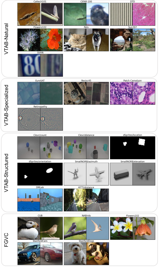
   Figure 10: Dataset examples for all classification tasks evaluated

   0.A.1.3 Augmentation and other hyper-parameters.

   We adopt standard image augmentation strategy during training: normalize with ImageNet means and standard deviation, randomly resize crop to 224$\times$224 and random horizontal flip for five FGVC datasets, and resize to 224$\times$224 for the VTAB-1k suite. Tab. 6 summarizes the optimization configurations we used. Following [56], we conduct grid search to find the tuning-specific hyper-parameters, learning rate, and weight decay values using val set of each task. Following the linear scaling rule [42, 27, 11, 30], the learning rate is set as base_lr$\times b/256$, where $b$ is the batch size used for the particular model, and base_lr is chosen from the range specified in Tab. 6. The optimal hyper-parameter values for each experiment can be found in Appendix 0.D.

   0.A.1.4 Datasets and pre-trained backbones specifications.

   Tabs. 7 and 8 summarize the statistics and details of the evaluated classification datasets and all the pre-trained backbones used in the paper. Fig. 10 includes image examples of all 24 classification tasks evaluated.

   0.A.2 Semantic Segmentation Experiments

   ADE20K [90] is a challenging scene parsing benchmark with 150 fine-grained labels. The training and validation sets contain 20,210 and 2,000 images respectively. We utilize the public codebase MMSegmentation [15] in our implementation. The ViT-L backbone is supervisely pre-trained on ImageNet-21k.

   SETR [89] is a competitive segmentation framework using ViT as the encoder. PUP is a progressive upsampling strategy consisting of consecutive convolution layers and bilinear upsampling operations. Among multiple decoder choices, PUP works the best according to MMSegmentation’s reproduction therefore we also use it as in our implementation.

   When applying VPT to SETR-PUP, we only insert prompts into SETR’s ViT encoder backbone. For the decoder, only image patch embeddings are used as inputs and prompt embeddings are discarded. Same as recognition tasks, only the PUP decoder head and prompts are learned during training and the ViT backbone is frozen.

   For full fine-tuning, we use the same hyper-parameters as in MMSegmentation. For HeadOnly, Bias, and VPT, we use the hyper-parameter sweep on learning rate {0.05, 0.005, 0.0005, 0.001}. The optimal learning rate is 0.005 for all methods. We sweep prompt length $p\in$ {1, 5, 10, 50, 100, 200}. For VPT, we also change the learning rate multiplier to 1.0 instead of the default 10.0, so the decoder head and prompts share the same learning rate. Other hyper-parameters remain the same as full fine-tuning.

   

   

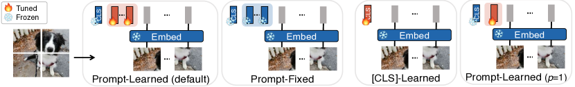
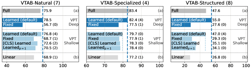
   Figure 11: Effect of expanding input sequence. Illustration of different strategies is included at top, and results of those are presented at the bottom section. For easy comparison, two dark and light blue lines represent the performance of default VPT-deep and VPT-shallow, respectively

   Appendix 0.B Extended Analysis

   0.B.0.1 Effect of expanding input sequence length.

   As shown in Tab. 1, by expanding the input sequence with learnable prompts, VPT achieves better performance than Full on the 20 out of 24 tasks evaluated. To investigate whether the advantage of VPT is due to its enlarged input sequence length, we experiment on two more variants: (1) the prompts are kept frozen during fine-tuning stage (Prompt-Fixed). (2) only tuning the [CLS] token ([CLS]-Learned). From Fig. 11 we can see that, updating prompt embeddings (Prompt-Learned) offers significant gains, while Prompt-Fixed yields comparable results w.r.t. Linear. This suggests that the final performance of VPT is mainly contributed by the learned prompt embeddings instead of the enlarged sequence length. Updating the [CLS] token performs similarly as updating 1 prompt ([CLS] vs. Learned_p=1), but still lags behind the default setting where we manually select the best number of prompt tokens based on the val set.

   

   

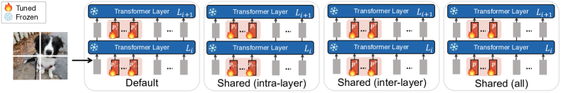
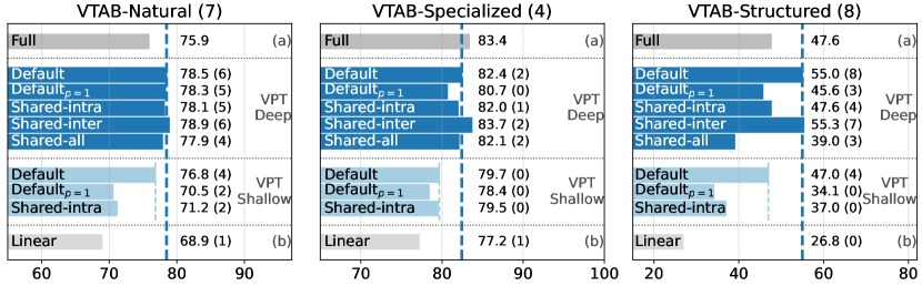
   Figure 12: Effect of sharing prompts. Illustration of different strategies is included at top, and results of those are presented at the bottom section. For easy comparison, the blue dashed line represents the performance of default VPT-deep

   0.B.0.2 Sharing prompts.

   We examine the effect of sharing parameters of prompts in Fig. 12 by setting the same prompt embedding within Transformer layers (Shared-intra), among all layers (Shared-inter), and for all prompts inserted in the Transformer (Shared-all). We can observe that: (1) Sharing prompts within layer (Shared-intra) performs competitively or slightly outperforms the performance of using one prompt (Default_p=1), further demonstrating the value of expanding input sequence. (2) Although Shared-intra under-performs Default in general, surprisingly, Shared-inter slightly outperforms our default VPT-deep while using similar number of trainable parameters (total number of parameters for all VTAB tasks: 1.14$\times$ vs. 1.13$\times$ for Shared-inter vs. Default, respectively). Closer examination reveals that the optimal prompt length $p$ for Shared-inter is in general larger than Default, i.e., average prompt length on all VTAB tasks: 64.58 vs. 60.94, for Shared-inter vs. Default, respectively. (3) Sharing the same prompt embedding both among and within layers (Shared-all) deteriorates performance, but still surpass the linear probing results across three VTAB subgroups.

   0.B.0.3 Prompt initialization.

   In NLP, prompt tuning could benefit from more sophisticated prompt initialization, as shown in [45]. We investigate if this is the case for visual prompting as well. We utilize prototype representations for downstream target classes so that the prompts are initialized with embeddings that enumerate the output space. Since we want the model to produce an output embedding that is close to one of these prototype representations given a test example, initializing prompts in this manner might give the model some hints about the target categories thus help improve the optimization process.

   Concretely, we use the averaged final [CLS] embeddings whithin each target class of the down-stream dataset train split. Given the pre-trained ViT with $N$ layers, and the down-stream train set with $c$ target classes, for each training example, we compute the final [CLS] embeddings, $\mathbf{x}_{N}\in\mathbb{R}^{d}$. Then we average these embeddings within each target class to get $\{\hat{\mathbf{x}}_{N}^{k}\in\mathbb{R}^{d}\mid k\in\mathbb{N},1\leq k\leq c\}$. Setting prompt length $p=c$, we initialize $\mathbf{P}$ with $\{\hat{\mathbf{x}}_{N}^{k}\}_{k=1}^{k=c}$ for VPT-shallow , and initialize each $\mathbf{P}_{i}$ with $\{\hat{\mathbf{x}}_{N}^{k}\}_{k=1}^{k=c}$, where $i=0,1,\ldots,N-1$, for VPT-deep.

   We compare the fine-tuning performance using the above initialization strategy (CLS) against the default random initialization (Random) in Fig. 13. We also report results when we fix the prompts during the fine-tuning stage ($\cdot$-fixed). As shown in Fig. 13, it’s quite surprising that our default random initialization (Random) works the best in general, consistently across different subgroups of VTAB without extra pre-processing steps described above (CLS). CLS works comparably in Natural and Specialized subgroups.

   

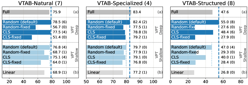
   Figure 13: Effect of prompt initialization. For easy comparison, the two blue dashed line represents the performance of default VPT-deep and VPT-shallow, respectively

   

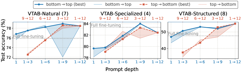
   Figure 14: Sensitivity to prompt length for the prompt depth experiments. We select the best prompt length for each variant with val sets. We also include the same prompt length for all depth choices. $i\rightarrow j$ indicates the Transformer layer indices that prompts are inserted into. The 1-st layer refers to the one closest to input. ViT-B has a total of 12 layers

   0.B.0.4 Prompt depth vs. prompt length.

   In Fig. 7, we ablate the number of layers we insert prompts in. For each prompt depth variant, Fig. 7 reports the results using the best prompt length for each task (“$\cdot\rightarrow\cdot$ (best)” in Fig. 14). Here we adopt another setting where the best prompt length from $1\rightarrow 12$ are used for all other prompt depth variants. Comparing both “$\cdot\rightarrow\cdot$ (best)” and “$\cdot\rightarrow\cdot$”, we observe that there are varied sensitivities to prompt length for different depths, especially if we insert prompts in nine layers only ($3\rightarrow$12, $12\rightarrow 3$).

   Table 9: Combining VPT with Bias with a pre-trained ViT-B in Sec. 4.2. For each method and each downstream task group, we report the average test accuracy score and number of wins in ($\cdot$) compared to Full. The difference between the hybrid methods and their VPT counterpart are color coded

   	Bias	VPT-shallow	VPT-shallow + Bias	VPT-deep	VPT-deep + Bias
   VTAB-Natural	73.30 (3)	76.81 (4)	79.78 (5) $\uparrow$2.97	78.48 (6)	77.64 (6) $\downarrow$0.84
   VTAB-Specialized	78.25 (0)	79.66 (0)	81.38 (0) $\uparrow$1.72	82.43 (2)	82.22 (2) $\downarrow$0.21
   VTAB-Structured	44.09 (2)	46.98 (4)	45.89 (3) $\downarrow$1.09	54.98 (8)	53.87 (6) $\downarrow$1.11

   

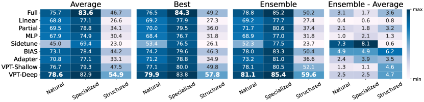
   Figure 15: Performance of a five-run ensemble. We report the averaged, the best among five runs as well. Best performance is bolded in each column

   0.B.0.5 Combine VPT with Bias Tuning.

   Our experiments in the main paper reveal that Bias is a competitive parameter-efficient tuning baseline (e.g., Tab. 1(c)). Based on this observation, we explore another protocol where we update both prompts and the bias terms of the pre-trained backbone, keeping everything else in the backbone frozen (VPT+Bias). As shown in Tab. 9, to our surprise, incorporating Bias with VPT does not yield superior results in general, even undermines VPT-deep for all 3 task subgroups. This suggests that these two methods are not necessarily complementary to each other.

   0.B.0.6 Prompt ensembling.

   [45] demonstrated prompt’s efficiency in the context of model ensembling. For an ensemble of $k$ models, we only need to store the learnt prompt vectors instead of $k$ copies of the whole fine-tuned model parameters (e.g., $k\times 2.5$GB for ViT-H). Furthermore, given one test example during inference time, only one forward pass is executed with a specially-designed batch with replicated original data but varied prompts.

   Given such advantages, we also investigate VPT’s effectiveness on prompt ensembling. We train 5 different prompts for each VTAB task with different random seeds, using the same pre-trained ViT-B backbone and hyper-parameters as in Tab. 1. Fig. 15 shows that the ensembled VPT-deep outperforms the average or even the best single-prompt counterparts, as well as other ensembled fine-tuning methods including Full.

   Table 10: Non-parametric paired one-tailed $t$-test (the Wilcoxon signed-rank test) on whether VPT-deep’s performance is greater than other methods on 19 VTAB tasks. Results show that, VPT-deep is indeed statistically significantly better than other fine-tuning protocols ($p<0.05$)

   	(a)	(b)			(c)			(ours)
   	Full	Linear	Mlp-3	Partial-1	Sidetune	Bias	Adapter	VPT-shallow
   Is VPT-deep statistically significantly better?	✓	✓	✓	✓	✓	✓	✓	✓
   $p$-value	1.2e-03	2.7e-05	1.9e-06	1.9e-05	1.9e-06	1.9e-06	3.8e-06	2.7e-05

   

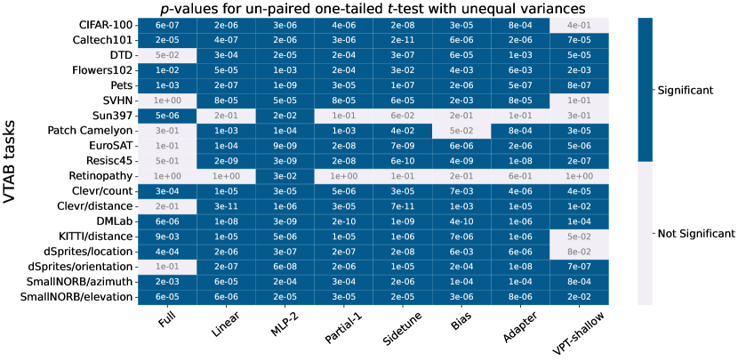
   Figure 16: Un-paired one-tailed $t$-test with unequal variances (Welch’s $t$-test) on whether VPT-deep’s performance is greater than other methods for each VTAB task. Results show that, VPT-deep is statistically significantly better than other fine-tuning protocols ($p<0.05$) in most instances

   

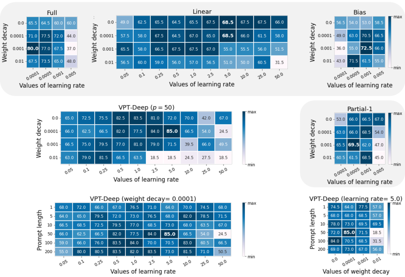
   Figure 17: Effect of different fine-tuning hyperparameters. Evaluated on the VTAB-Specialized: KITTI/Distance task. Other tuning methods are shaded in gray

   0.B.0.7 Test of statistical significance.

   We conduct non-parametric paired one-tailed $t$-test (the Wilcoxon signed-rank test [82]) on whether VPT-deep’s performance is greater than other fine-tuning methods across 19 VTAB tasks (the null hypothesis $H_{0}$ states that the mean VTAB performance difference between VPT-deep and alternate baseline method is zero. The alternative hypothesis $H_{1}$ states that VPT-deep outperforms the baseline method on VTAB). Tab. 10 presents the $p$-values of each test, with the number of observations equal to 19 for each method compared (we use the averaged accuracy scores among 5 runs for 19 VTAB tasks and all fine-tuning methods). For all of the fine-tuning protocols compared, VPT-deep’s improvements are statistically significant ($p<0.05$).

   We also conduct un-paired one-tailed $t$-test with unequal variances (Welch’s $t$-test [81]), comparing the individual runs (the number of observations = 5) for each VTAB task ($H_{0}$ states that VPT-deep and the other baseline perform the same for a specific VTAB task, while $H_{1}$ states that VPT-deep outperforms the other baseline for a specific VTAB task). Fig. 16 presents the $p$-values for each $<$VPT-deep, baseline method$>$ pair on each task. We reject $H_{0}$ on 127 out of $19\times 8=152$ cases ($p<0.05$). Compared to Full, VPT-deep achieves statistically significant better performance on 11 out of 19 tasks.

   Table 11: ViT-B/16 pre-trained on supervised ImageNet-21k, fine-tuned with resolution 384$\times$384. We also include VPT with image resolution 224$\times$224, $p=380$, so the effective image resolution is 384$\times$384. For each method and each downstream task group, we report the average test accuracy score and number of wins in ($\cdot$) compared to Full. “Total params” denotes total parameters needed for all 24 downstream tasks. Best results among all methods except Full are bolded

   	ViT-B/16	Fine-tune	Total	VTAB-1k
   	(85.8M)	Resolution	params	Natural	Specialized	Structured
   	Total # of tasks			7	4	8
   (a)	Full	384	19.07$\times$	72.57	83.05	50.86
   	Full	224	19.07$\times$	75.88	83.36	47.64
   (b)	Linear		1.01$\times$	66.30 (2)	76.77 (0)	27.86 (0)
   	Mlp-3	384	1.27$\times$	66.45 (3)	77.77 (0)	38.03 (0)
   	Partial-1		2.58$\times$	67.91 (4)	76.94 (0)	37.16 (0)
   	Sidetune		3.12$\times$	47.08 (1)	40.34 (0)	24.18 (0)
   (c)	Bias	384	1.03$\times$	70.30 (4)	76.06 (0)	45.35 (1)
   	Adapter		1.11$\times$	69.42 (6)	77.11 (0)	30.62 (0)
   (ours)	VPT-shallow ($p\in\{1,5,10,50,100,200\}$)	384	1.02$\times$	75.30 (4)	78.50 (0)	46.56 (2)
   	VPT-deep ($p\in\{1,5,10,50,100,200\}$)	384	1.19$\times$	79.37 (6)	82.86 (2)	56.36 (7)
   	VPT-shallow ($p=380$)	224	1.07$\times$	75.07 (3)	79.03 (0)	46.21 (2)
   	VPT-deep ($p=380$)	224	1.78$\times$	74.20 (4)	82.30 (2)	54.50 (6)

   0.B.0.8 Effect of different fine-tuning hyper-parameters.

   In Fig. 17, we present different tuning protocol’s performance on different fine-tuning hyper-parameters including learning rate and weight decay. For our proposed VPT-deep, we also ablate different choices of prompt length $p$, which is the only hyper-parameter that needs to be manually tuned. All experiments are evaluated on the val set of KITTI/Distance task (VTAB-Specialized). We observe different behaviors between Linear and VPT. Both methods freeze backbone parameters during fine-tuning stage. Linear probing is more sensitive to weight decay values in general, whereas VPT is influenced by both learning rate and weight decay values. VPT with larger prompt length is also less sensitive to the choice of learning rate.

   0.B.0.9 Effect of image resolution.

   The original ViT paper [19] found that fine-tuning with higher image resolutions (384$\times$384) is beneficial to downstream recognition tasks. All recognition experiments presented in the main paper are fine-tuned on 224$\times$224 resolution. As shown in Tab. 11, we re-run the VTAB experiments with the same setup as in Tab. 1 but in the 384 resolution instead of the default 224. We can see that, VPT-deep still achieves the best performance among all parameter-efficient tuning protocols, and even outperforms full fine-tuning on 15 out of 19 tasks. Although the increase of image resolutions doesn’t lead to better full fine-tuning performance in general, it indeed slightly boosts VPT-deep’s performance.

   Another interesting observation from Tab. 11 is that with 224 fine-tune resolution and a larger value of $p=380$, VPT could achieve similar or better performance compared to Full with 384 resolution, while using the same input sequence length yet significantly less trainable parameters.

   0.B.0.10 Empirical computational cost.

   One possible limitation of VPT is the extra input sequence length for Transformers. In theory the complexity of MSA is quadratic w.r.t. the input sequence length, but this might not be the case for real-world speed due to hardware details like lane widths and cache sizes [19]. In Tabs. 12 and 18, we study the empirical computational cost, i.e., latency, and peak GPU memory usage at both training and inference times, for all the fine-tuning protocols studied. All experiments use the same A100 GPU with a batch size 64 for both training and inference. We can see that the theoretical quadratic scaling w.r.t. sequence length barely happens to VPT. For instance, doubling the length ($p=200$ vs. $m=198$) basically only lead to 2$\times$ (instead of 4$\times$) inference latency and peak GPU memory w.r.t. full fine-tuning. For training, the latency would be largely reduced with less number of prompts.

   An equivalent implementation of VPT during test time is directly prepend the parameters to the key and value arrays inside the self-attention module of Transformer [48] (VPT-prefix). While we found that such implementation does not lead to accuracy improvement on VTAB datasets, it reduces the computation cost during inference. Figure 19 shows the comparison with different values of $p$. VPT-prefix reduces test-time latency and peak GPU memory with a large margin especially when $p$ becomes large.

   Table 12: Cost analysis using a ViT-B/16 pre-trained on supervised ImageNet-21k. For each method and each downstream task group, we report the latency (ms/img) and peak GPU memory usage (GB) at both training and inference time. “Tuned params” denotes the fraction of learnable parameters needed. “Scope” denotes the tuning scope of each method. “Extra params” denotes the presence of additional parameters besides the pre-trained backbone and linear head. All experiments use the same A100 GPU

   	ViT-B/16	Tuned	Scope			Extra	Train		Test
   	(85.8M)	params	Input	Backbone	Head	params	Latency	Memory	Latency	Memory
   							(ms/img)	(GB)	(ms/img)	(GB)
   (a)	Full	100$\%$		✓	✓		358.7	11.7	69.7	0.87
   (b)	Linear	0.09$\%$					148.9	0.9	64.4	0.87
   	Partial-1	8.35$\%$			✓		193.2	1.4	66.1	0.87
   	Mlp-3	1.45$\%$				✓	164.3	0.9	64.4	0.87
   (c)	Sidetune	10.09$\%$		✓		✓	164.6	1.2	66.9	0.91
   	Bias	0.21$\%$					296.9	10.1	65.6	0.87
   	Adapter ($r=8$)	2.12$\%$				✓	293.4	9.9	68.2	0.87
   	Adapter ($r=64$)	0.36$\%$				✓	294.4	9.8	68.3	0.87
   	Adapter ($r=256$)	0.17$\%$				✓	271.4	9.8	68.0	0.87
   (ours)	VPT-shallow ($p=1$)	0.09$\%$	✓			✓	205.9	10.3	68.1	0.88
   	VPT-deep ($p=1$)	0.10$\%$					213.6	10.3	69.4	0.88
   	VPT-shallow ($p=200$)	0.27$\%$					350.6	25.8	138.8	1.84
   	VPT-deep ($p=200$)	2.19$\%$					360.1	25.8	140.8	1.85

   

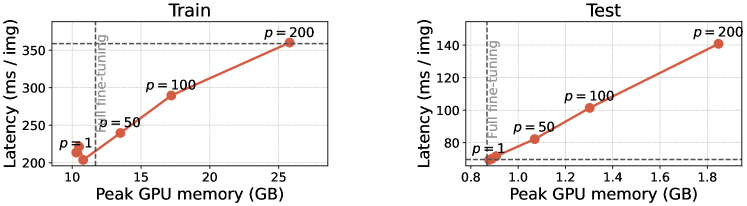
   Figure 18: Peak GPU memory and latency (ms/img) during both training (left) and inference time (right). For easy comparison, the gray dashed lines represent latency and memory of full fine-tuning

   

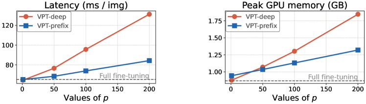
   Figure 19: VPT-deep vs. VPT-prefix: peak GPU memory (left) and latency (right) during inference time. For easy comparison, the gray dashed lines represent latency and memory of full fine-tuning

   Appendix 0.C Further Discussion

   0.C.0.1 VPT vs. Adversarial Reprogramming (AR).

   The differences are: (1) the number of learnt parameters injected in the input space in AR literature [20] is nearly 20 times larger than ours (264k vs. 13k). VPT is significantly more parameter-efficient; (2) AR has shown its effectiveness in ConvNet, while VPT can be applied to broader architectures, including ViT, Swin. Furthermore, VPT is more general with the option of diving into deeper layers of pre-trained backbone (Fig. 2), whereas AR strictly applies to the first input layer of ConvNets. (3) another distinction is that our setting update both prompts and classification head, while AR [20] directly use the pre-trained classification head. Our setup is more general and could be applied to models with a broader range of pre-training objectives (e.g., MAE [30], which does not include a pre-trained classification head) and broader vision tasks (e.g., segmentation).

   0.C.0.2 Visual prompt vs. textual prompt.

   Our paper also discover discrepancies between visual and textual prompts: we show that VPT could even outperform full-model fine-tuning on 20 out of 24 cases, which is in contract to the NLP’s related work [45]. We also found that random initialized prompts works better in Fig. 13, and prompts at earlier layers matters more (Figs. 7 and 14), which are also different from observation on the NLP side [45, 51]. These discrepancies indicate that visual prompting might be fundamentally different from text prompts thus in need of further investigation.

   Appendix 0.D Supplementary Results

   Table 13: Per-task fine-tuning results from Tab. 1 for VTAB-1k with a pre-trained ViT-B/16

   		CIFAR-100	Caltech101	DTD	Flowers102	Pets	SVHN	Sun397	Mean	Patch Camelyon	EuroSAT	Resisc45	Retinopathy	Mean	Clevr/count	Clevr/distance	DMLab	KITTI/distance	dSprites/location	dSprites/orientation	SmallNORB/azimuth	SmallNORB/elevation	Mean
   (a)	Full	68.9	87.7	64.3	97.2	86.9	87.4	38.8	75.88	79.7	95.7	84.2	73.9	83.36	56.3	58.6	41.7	65.5	57.5	46.7	25.7	29.1	47.64
   Head-oriented
   (a)	Linear	63.4	85.0	63.2	97.0	86.3	36.6	51.0	68.93 (1)	78.5	87.5	68.6	74.0	77.16 (1)	34.3	30.6	33.2	55.4	12.5	20.0	9.6	19.2	26.84 (0)
   	Partial-1	66.8	85.9	62.5	97.3	85.5	37.6	50.6	69.44 (2)	78.6	89.8	72.5	73.3	78.53 (0)	41.5	34.3	33.9	61.0	31.3	32.8	16.3	22.4	34.17 (0)
   	Mlp-2	63.2	84.8	60.5	97.6	85.9	34.1	47.8	67.70 (2)	74.3	88.8	67.1	73.2	75.86 (0)	45.2	31.6	31.8	55.7	30.9	24.6	16.6	23.3	32.47 (0)
   	Mlp-3	63.8	84.7	62.3	97.4	84.7	32.5	49.2	67.80 (2)	77.0	88.0	70.2	56.1	72.83 (0)	47.8	32.8	32.3	58.1	12.9	21.2	15.2	24.8	30.62 (0)
   	Mlp-5	59.3	84.4	59.9	96.1	84.4	30.9	46.8	65.98 (1)	73.7	87.2	64.8	71.5	74.31 (0)	50.8	32.3	31.5	56.4	7.5	20.8	14.4	20.4	29.23 (0)
   	Mlp-9	53.1	80.5	53.9	95.1	82.6	24.4	43.7	61.90 (1)	78.5	83.0	60.2	72.3	73.49 (0)	47.5	27.9	28.9	54.0	6.2	17.7	10.8	16.2	26.15 (0)
   Backbone-oriented
   (b)	Sidetune	60.7	60.8	53.6	95.5	66.7	34.9	35.3	58.21 (0)	58.5	87.7	65.2	61.0	68.12 (0)	27.6	22.6	31.3	51.7	8.2	14.4	9.8	21.8	23.41 (0)
   	Bias	72.8	87.0	59.2	97.5	85.3	59.9	51.4	73.30 (3)	78.7	91.6	72.9	69.8	78.25 (0)	61.5	55.6	32.4	55.9	66.6	40.0	15.7	25.1	44.09 (2)
   	Adapter-256	74.1	86.1	63.2	97.7	87.0	34.6	50.8	70.50 (4)	76.3	88.0	73.1	70.5	76.98 (0)	45.7	37.4	31.2	53.2	30.3	25.4	13.8	22.1	32.39 (0)
   	Adapter-64	74.2	85.8	62.7	97.6	87.2	36.3	50.9	70.65 (4)	76.3	87.5	73.7	70.9	77.10 (0)	42.9	39.9	30.4	54.5	31.9	25.6	13.5	21.4	32.51 (0)
   	Adapter-8	74.2	85.7	62.7	97.8	87.2	36.4	50.7	70.67 (4)	76.9	89.2	73.5	71.6	77.80 (0)	45.2	41.8	31.1	56.4	30.4	24.6	13.2	22.0	33.09 (0)
   Visual-Prompt Tuning
   (ours)	VPT-shallow	77.7	86.9	62.6	97.5	87.3	74.5	51.2	76.81 (4)	78.2	92.0	75.6	72.9	79.66 (0)	50.5	58.6	40.5	67.1	68.7	36.1	20.2	34.1	46.98 (4)
   	Prompt length ($p$)	100	5	1	200	50	200	1	79.4	5	50	50	10	28.7	100	200	100	100	100	100	200	200	137.5
   	Tuned / Total (%)	0.18	0.10	0.04	0.27	0.08	0.19	0.36	0.17	0.01	0.05	0.09	0.01	0.04	0.10	0.18	0.09	0.09	0.10	0.10	0.19	0.19	0.13
   	VPT-deep	78.8	90.8	65.8	98.0	88.3	78.1	49.6	78.48 (6)	81.8	96.1	83.4	68.4	82.43 (2)	68.5	60.0	46.5	72.8	73.6	47.9	32.9	37.8	54.98 (8)
   	Prompt length ($p$)	10	10	10	1	1	50	5	12.4	100	100	10	1	52.8	50	200	100	50	10	50	200	200	107.5
   	Tuned / Total (%)	0.20	0.20	0.15	0.10	0.04	0.54	0.41	0.23	1.06	1.07	0.15	0.02	0.57	0.54	2.11	1.07	0.54	0.12	0.55	2.12	2.11	1.14

   Table 14: Per-task fine-tuning results from Tab. 1 for five FGVC tasks, with a pre-trained ViT-B/16

   		CUB-200-2011	NABirds	Oxford Flowers	Stanford Dogs	Stanford Cars	Mean
   (a)	Full	87.3	82.7	98.8	89.4	84.5	88.54
   Head-oriented
   (a)	Linear	85.3	75.9	97.9	86.2	51.3	79.32 (0)
   	Partial-1	85.6	77.8	98.2	85.5	66.2	82.63 (0)
   	Mlp-2	85.7	77.2	98.2	85.4	54.9	80.28 (0)
   	Mlp-3	85.1	77.3	97.9	84.9	53.8	79.80 (0)
   	Mlp-5	84.2	76.7	97.6	84.8	50.2	78.71 (0)
   	Mlp-9	83.2	76.0	96.2	83.7	47.6	77.31 (0)
   Backbone-oriented
   (b)	Sidetune	84.7	75.8	96.9	85.8	48.6	78.35 (0)
   	Bias	88.4	84.2	98.8	91.2	79.4	88.41 (3)
   	Adapter-256	87.2	84.3	98.5	89.9	68.6	85.70 (2)
   	Adapter-64	87.1	84.3	98.5	89.8	68.6	85.67 (2)
   	Adapter-8	87.3	84.3	98.4	88.8	68.4	85.46 (1)
   Visual-Prompt Tuning
   (ours)	VPT-shallow	86.7	78.8	98.4	90.7	68.7	84.62 (1)
   	Prompt length ($p$)	100	50	100	100	100	90
   	Tuned / Total (%)	0.31	0.54	0.23	0.20	0.26	0.31
   	VPT-deep	88.5	84.2	99.0	90.2	83.6	89.11 (4)
   	Prompt length ($p$)	10	50	5	100	200	73
   	Tuned / Total (%)	0.29	1.02	0.14	1.17	2.27	0.98

   0.D.0.1 Numerical results of Table 1.

   Tabs. 13 and 14 present per-task results for 24 classification tasks evaluated in Tab. 1.

   0.D.0.2 Per-task results on training data ablations.

   Fig. 20 presents the per-task results for five FGVC datasets. We observe a similar trend in Fig. 3: while all parameter-efficient methods outperform full fine-tuning in small-to-medium data regime, VPT-deep consistently surpasses Full across data scales for five FGVC tasks.

   

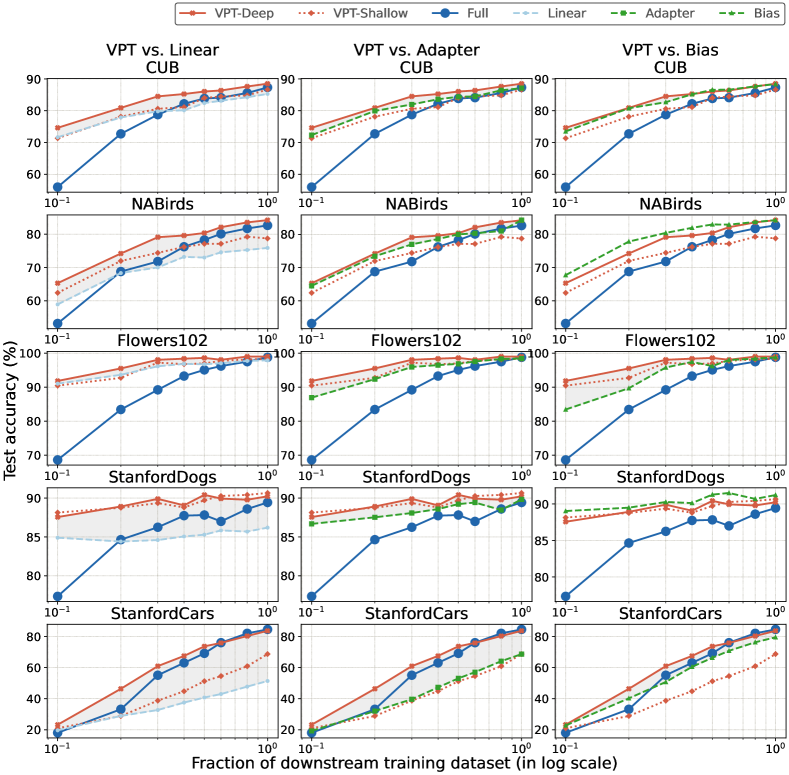
   Figure 20: Effect of downstream data size, for each of FGVC tasks. The size of markers are proportional to the percentage of tunable parameters in log scale

   

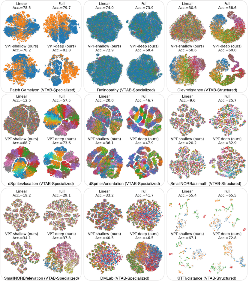
   Figure 21: More t-SNE visualization of the final [CLS] embedding $\mathbf{x}_{N}$ of more VTAB tasks. We include tasks that have less or equal to 20 target classes for visualization

   0.D.0.3 More t-SNE visualizations.

   In Fig. 21, We presents more t-SNE visualizations, similar to Fig. 9, for all VTAB datasets with less than or equal to 20 target classes.

References

- [1] Ba, J.L., Kiros, J.R., Hinton, G.E.: Layer normalization. arXiv preprint arXiv:1607.06450 (2016)
- [2] Bahng, H., Jahanian, A., Sankaranarayanan, S., Isola, P.: Visual prompting: Modifying pixel space to adapt pre-trained models. arXiv preprint arXiv:2203.17274 (2022)
- [3] Bao, H., Dong, L., Piao, S., Wei, F.: BEit: BERT pre-training of image transformers. In: ICLR (2022)
- [4] Beattie, C., Leibo, J.Z., Teplyashin, D., Ward, T., Wainwright, M., Küttler, H., Lefrancq, A., Green, S., Valdés, V., Sadik, A., et al.: Deepmind lab. arXiv preprint arXiv:1612.03801 (2016)
- [5] Ben Zaken, E., Goldberg, Y., Ravfogel, S.: BitFit: Simple parameter-efficient fine-tuning for transformer-based masked language-models. In: Proceedings of the 60th Annual Meeting of the Association for Computational Linguistics (Volume 2: Short Papers). pp. 1–9. Association for Computational Linguistics, Dublin, Ireland (May 2022). https://doi.org/10.18653/v1/2022.acl-short.1, https://aclanthology.org/2022.acl-short.1
- [6] Bommasani, R., Hudson, D.A., Adeli, E., Altman, R., Arora, S., von Arx, S., Bernstein, M.S., Bohg, J., Bosselut, A., Brunskill, E., et al.: On the opportunities and risks of foundation models. arXiv preprint arXiv:2108.07258 (2021)
- [7] Brown, T., Mann, B., Ryder, N., Subbiah, M., Kaplan, J.D., Dhariwal, P., Neelakantan, A., Shyam, P., Sastry, G., Askell, A., Agarwal, S., Herbert-Voss, A., Krueger, G., Henighan, T., Child, R., Ramesh, A., Ziegler, D., Wu, J., Winter, C., Hesse, C., Chen, M., Sigler, E., Litwin, M., Gray, S., Chess, B., Clark, J., Berner, C., McCandlish, S., Radford, A., Sutskever, I., Amodei, D.: Language models are few-shot learners. In: Larochelle, H., Ranzato, M., Hadsell, R., Balcan, M.F., Lin, H. (eds.) NeurIPS. vol. 33, pp. 1877–1901. Curran Associates, Inc. (2020)
- [8] Cai, H., Gan, C., Zhu, L., Han, S.: Tinytl: Reduce memory, not parameters for efficient on-device learning. NeurIPS 33, 11285–11297 (2020)
- [9] Carion, N., Massa, F., Synnaeve, G., Usunier, N., Kirillov, A., Zagoruyko, S.: End-to-end object detection with transformers. In: ECCV. pp. 213–229. Springer (2020)
- [10] Chen, L.C., Zhu, Y., Papandreou, G., Schroff, F., Adam, H.: Encoder-decoder with atrous separable convolution for semantic image segmentation. In: ECCV. pp. 801–818 (2018)
- [11] Chen*, X., Xie*, S., He, K.: An empirical study of training self-supervised vision transformers. In: ICCV (2021)
- [12] Cheng, G., Han, J., Lu, X.: Remote sensing image scene classification: Benchmark and state of the art. Proceedings of the IEEE (2017)
- [13] Cimpoi, M., Maji, S., Kokkinos, I., Mohamed, S., , Vedaldi, A.: Describing textures in the wild. In: CVPR (2014)
- [14] Conder, J., Jefferson, J., Jawed, K., Nejati, A., Sagar, M., et al.: Efficient transfer learning for visual tasks via continuous optimization of prompts. In: International Conference on Image Analysis and Processing. pp. 297–309. Springer (2022)
- [15] Contributors, M.: MMSegmentation: Openmmlab semantic segmentation toolbox and benchmark. https://github.com/open-mmlab/mmsegmentation (2020)
- [16] Deng, J., Dong, W., Socher, R., Li, L.J., Li, K., Fei-Fei, L.: Imagenet: A large-scale hierarchical image database. In: CVPR (2009)
- [17] Devlin, J., Chang, M.W., Lee, K., Toutanova, K.: BERT: Pre-training of deep bidirectional transformers for language understanding. In: Proceedings of the 2019 Conference of the North American Chapter of the Association for Computational Linguistics: Human Language Technologies, Volume 1 (Long and Short Papers). pp. 4171–4186. Association for Computational Linguistics, Minneapolis, Minnesota (Jun 2019)
- [18] Doersch, C., Gupta, A., Zisserman, A.: Crosstransformers: spatially-aware few-shot transfer. NeurIPS 33, 21981–21993 (2020)
- [19] Dosovitskiy, A., Beyer, L., Kolesnikov, A., Weissenborn, D., Zhai, X., Unterthiner, T., Dehghani, M., Minderer, M., Heigold, G., Gelly, S., et al.: An image is worth 16x16 words: Transformers for image recognition at scale. In: ICLR (2020)
- [20] Elsayed, G.F., Goodfellow, I., Sohl-Dickstein, J.: Adversarial reprogramming of neural networks. In: ICLR (2019)
- [21] Feichtenhofer, C., Fan, H., Li, Y., He, K.: Masked autoencoders as spatiotemporal learners. arXiv preprint arXiv:2205.09113 (2022)
- [22] Ge, C., Huang, R., Xie, M., Lai, Z., Song, S., Li, S., Huang, G.: Domain adaptation via prompt learning. arXiv preprint arXiv:2202.06687 (2022)
- [23] Gebru, T., Krause, J., Wang, Y., Chen, D., Deng, J., Fei-Fei, L.: Fine-grained car detection for visual census estimation. In: AAAI (2017)
- [24] Geiger, A., Lenz, P., Stiller, C., Urtasun, R.: Vision meets robotics: The kitti dataset. International Journal of Robotics Research (2013)
- [25] Girdhar, R., Carreira, J., Doersch, C., Zisserman, A.: Video action transformer network. In: CVPR. pp. 244–253 (2019)
- [26] Glorot, X., Bengio, Y.: Understanding the difficulty of training deep feedforward neural networks. In: AISTATS (2010)
- [27] Goyal, P., Dollár, P., Girshick, R., Noordhuis, P., Wesolowski, L., Kyrola, A., Tulloch, A., Jia, Y., He, K.: Accurate, large minibatch sgd: Training imagenet in 1 hour. arXiv preprint arXiv:1706.02677 (2017)
- [28] Guo, D., Rush, A., Kim, Y.: Parameter-efficient transfer learning with diff pruning. In: Proceedings of the 59th Annual Meeting of the Association for Computational Linguistics and the 11th International Joint Conference on Natural Language Processing (Volume 1: Long Papers). pp. 4884–4896. Association for Computational Linguistics, Online (Aug 2021)
- [29] He, J., Zhou, C., Ma, X., Berg-Kirkpatrick, T., Neubig, G.: Towards a unified view of parameter-efficient transfer learning. In: ICLR (2022)
- [30] He, K., Chen, X., Xie, S., Li, Y., Dollár, P., Girshick, R.: Masked autoencoders are scalable vision learners. In: CVPR. pp. 16000–16009 (2022)
- [31] He, K., Zhang, X., Ren, S., Sun, J.: Deep residual learning for image recognition. In: CVPR. pp. 770–778 (2016)
- [32] Helber, P., Bischke, B., Dengel, A., Borth, D.: Eurosat: A novel dataset and deep learning benchmark for land use and land cover classification. IEEE Journal of Selected Topics in Applied Earth Observations and Remote Sensing 12(7), 2217–2226 (2019)
- [33] Helber, P., Bischke, B., Dengel, A., Borth, D.: Eurosat: A novel dataset and deep learning benchmark for land use and land cover classification. IEEE Journal of Selected Topics in Applied Earth Observations and Remote Sensing (2019)
- [34] Houlsby, N., Giurgiu, A., Jastrzebski, S., Morrone, B., De Laroussilhe, Q., Gesmundo, A., Attariyan, M., Gelly, S.: Parameter-efficient transfer learning for nlp. In: ICML. pp. 2790–2799. PMLR (2019)
- [35] Hu, E.J., Shen, Y., Wallis, P., Allen-Zhu, Z., Li, Y., Wang, S., Wang, L., Chen, W.: Lora: Low-rank adaptation of large language models. arXiv preprint arXiv:2106.09685 (2021)
- [36] Jia, M., Wu, Z., Reiter, A., Cardie, C., Belongie, S., Lim, S.N.: Exploring visual engagement signals for representation learning. In: ICCV (2021)
- [37] Jiang, Z., Xu, F.F., Araki, J., Neubig, G.: How can we know what language models know? Transactions of the Association for Computational Linguistics 8, 423–438 (2020)
- [38] Johnson, J., Hariharan, B., van der Maaten, L., Fei-Fei, L., Lawrence Zitnick, C., Girshick, R.: Clevr: A diagnostic dataset for compositional language and elementary visual reasoning. In: CVPR (2017)
- [39] Ju, C., Han, T., Zheng, K., Zhang, Y., Xie, W.: Prompting visual-language models for efficient video understanding. arXiv preprint arXiv:2112.04478 (2021)
- [40] Kaggle, EyePacs: Kaggle diabetic retinopathy detection (July 2015)
- [41] Khosla, A., Jayadevaprakash, N., Yao, B., Fei-Fei, L.: Novel dataset for fine-grained image categorization. In: First Workshop on Fine-Grained Visual Categorization, IEEE Conference on Computer Vision and Pattern Recognition. Colorado Springs, CO (June 2011)
- [42] Krizhevsky, A.: One weird trick for parallelizing convolutional neural networks. arXiv preprint arXiv:1404.5997 (2014)
- [43] Krizhevsky, A., Hinton, G., et al.: Learning multiple layers of features from tiny images (2009)
- [44] LeCun, Y., Huang, F.J., Bottou, L.: Learning methods for generic object recognition with invariance to pose and lighting. In: CVPR (2004)
- [45] Lester, B., Al-Rfou, R., Constant, N.: The power of scale for parameter-efficient prompt tuning. In: Proceedings of the 2021 Conference on Empirical Methods in Natural Language Processing. pp. 3045–3059. Association for Computational Linguistics, Online and Punta Cana, Dominican Republic (Nov 2021)
- [46] Lewis, M., Liu, Y., Goyal, N., Ghazvininejad, M., Mohamed, A., Levy, O., Stoyanov, V., Zettlemoyer, L.: Bart: Denoising sequence-to-sequence pre-training for natural language generation, translation, and comprehension. In: Proceedings of the 58th Annual Meeting of the Association for Computational Linguistics. pp. 7871–7880 (2020)
- [47] Li, F.F., Fergus, R., Perona, P.: One-shot learning of object categories. IEEE TPAMI (2006)
- [48] Li, X.L., Liang, P.: Prefix-tuning: Optimizing continuous prompts for generation. In: Proceedings of the 59th Annual Meeting of the Association for Computational Linguistics and the 11th International Joint Conference on Natural Language Processing (Volume 1: Long Papers). pp. 4582–4597. Association for Computational Linguistics, Online (Aug 2021)
- [49] Li, Y., Xie, S., Chen, X., Dollar, P., He, K., Girshick, R.: Benchmarking detection transfer learning with vision transformers. arXiv preprint arXiv:2111.11429 (2021)
- [50] Liu, P., Yuan, W., Fu, J., Jiang, Z., Hayashi, H., Neubig, G.: Pre-train, prompt, and predict: A systematic survey of prompting methods in natural language processing. arXiv preprint arXiv:2107.13586 (2021)
- [51] Liu, X., Ji, K., Fu, Y., Du, Z., Yang, Z., Tang, J.: P-tuning v2: Prompt tuning can be comparable to fine-tuning universally across scales and tasks. arXiv preprint arXiv:2110.07602 (2021)
- [52] Liu, Z., Lin, Y., Cao, Y., Hu, H., Wei, Y., Zhang, Z., Lin, S., Guo, B.: Swin transformer: Hierarchical vision transformer using shifted windows. In: ICCV (2021)
- [53] Liu, Z., Mao, H., Wu, C.Y., Feichtenhofer, C., Darrell, T., Xie, S.: A convnet for the 2020s. CVPR (2022)
- [54] Loshchilov, I., Hutter, F.: Decoupled weight decay regularization. arXiv preprint arXiv:1711.05101 (2017)
- [55] Van der Maaten, L., Hinton, G.: Visualizing data using t-sne. Journal of machine learning research 9(11) (2008)
- [56] Mahajan, D., Girshick, R., Ramanathan, V., He, K., Paluri, M., Li, Y., Bharambe, A., Van Der Maaten, L.: Exploring the limits of weakly supervised pretraining. In: ECCV (2018)
- [57] Matthey, L., Higgins, I., Hassabis, D., Lerchner, A.: dsprites: Disentanglement testing sprites dataset. https://github.com/deepmind/dsprites-dataset/ (2017)
- [58] Netzer, Y., Wang, T., Coates, A., Bissacco, A., Wu, B., Ng, A.Y.: Reading digits in natural images with unsupervised feature learning. In: NIPS Workshop on Deep Learning and Unsupervised Feature Learning 2011 (2011)
- [59] Nilsback, M.E., Zisserman, A.: Automated flower classification over a large number of classes. In: 2008 Sixth Indian Conference on Computer Vision, Graphics & Image Processing. pp. 722–729. IEEE (2008)
- [60] Noroozi, M., Favaro, P.: Unsupervised learning of visual representations by solving jigsaw puzzles. In: ECCV. pp. 69–84. Springer (2016)
- [61] Parkhi, O.M., Vedaldi, A., Zisserman, A., Jawahar, C.V.: Cats and dogs. In: CVPR (2012)
- [62] Paszke, A., Gross, S., Chintala, S., Chanan, G., Yang, E., DeVito, Z., Lin, Z., Desmaison, A., Antiga, L., Lerer, A.: Automatic differentiation in PyTorch. In: NeurIPS Autodiff Workshop (2017)
- [63] Pfeiffer, J., Kamath, A., Rücklé, A., Cho, K., Gurevych, I.: Adapterfusion: Non-destructive task composition for transfer learning. arXiv preprint arXiv:2005.00247 (2020)
- [64] Pfeiffer, J., Rücklé, A., Poth, C., Kamath, A., Vulić, I., Ruder, S., Cho, K., Gurevych, I.: Adapterhub: A framework for adapting transformers. In: Proceedings of the 2020 Conference on Empirical Methods in Natural Language Processing (EMNLP 2020): Systems Demonstrations. pp. 46–54. Association for Computational Linguistics, Online (2020)
- [65] Radford, A., Kim, J.W., Hallacy, C., Ramesh, A., Goh, G., Agarwal, S., Sastry, G., Askell, A., Mishkin, P., Clark, J., et al.: Learning transferable visual models from natural language supervision. In: International Conference on Machine Learning. pp. 8748–8763. PMLR (2021)
- [66] Raffel, C., Shazeer, N., Roberts, A., Lee, K., Narang, S., Matena, M., Zhou, Y., Li, W., Liu, P.J.: Exploring the limits of transfer learning with a unified text-to-text transformer. Journal of Machine Learning Research 21(140), 1–67 (2020)
- [67] Rebuffi, S.A., Bilen, H., Vedaldi, A.: Learning multiple visual domains with residual adapters. NeurIPS 30 (2017)
- [68] Rebuffi, S.A., Bilen, H., Vedaldi, A.: Efficient parametrization of multi-domain deep neural networks. In: CVPR. pp. 8119–8127 (2018)
- [69] Sandler, M., Zhmoginov, A., Vladymyrov, M., Jackson, A.: Fine-tuning image transformers using learnable memory. In: CVPR. pp. 12155–12164 (2022)
- [70] Shin, T., Razeghi, Y., Logan IV, R.L., Wallace, E., Singh, S.: Autoprompt: Eliciting knowledge from language models with automatically generated prompts. arXiv preprint arXiv:2010.15980 (2020)
- [71] Strudel, R., Garcia, R., Laptev, I., Schmid, C.: Segmenter: Transformer for semantic segmentation. In: CVPR. pp. 7262–7272 (2021)
- [72] Van Horn, G., Branson, S., Farrell, R., Haber, S., Barry, J., Ipeirotis, P., Perona, P., Belongie, S.: Building a bird recognition app and large scale dataset with citizen scientists: The fine print in fine-grained dataset collection. In: CVPR. pp. 595–604 (2015)
- [73] Vaswani, A., Shazeer, N., Parmar, N., Uszkoreit, J., Jones, L., Gomez, A.N., Kaiser, Ł., Polosukhin, I.: Attention is all you need. NeurIPS 30 (2017)
- [74] Veeling, B.S., Linmans, J., Winkens, J., Cohen, T., Welling, M.: Rotation equivariant cnns for digital pathology. In: International Conference on Medical Image Computing and Computer-Assisted Intervention (2018)
- [75] Wah, C., Branson, S., Welinder, P., Perona, P., Belongie, S.: The caltech-ucsd birds-200-2011 dataset. Tech. Rep. CNS-TR-2011-001, California Institute of Technology (2011)
- [76] Wang, A., Pruksachatkun, Y., Nangia, N., Singh, A., Michael, J., Hill, F., Levy, O., Bowman, S.: Superglue: A stickier benchmark for general-purpose language understanding systems. NeurIPS 32 (2019)
- [77] Wang, A., Singh, A., Michael, J., Hill, F., Levy, O., Bowman, S.: GLUE: A multi-task benchmark and analysis platform for natural language understanding. In: Proceedings of the 2018 EMNLP Workshop BlackboxNLP: Analyzing and Interpreting Neural Networks for NLP. pp. 353–355. Association for Computational Linguistics, Brussels, Belgium (Nov 2018). https://doi.org/10.18653/v1/W18-5446, https://aclanthology.org/W18-5446
- [78] Wang, H., Zhu, Y., Adam, H., Yuille, A., Chen, L.C.: Max-deeplab: End-to-end panoptic segmentation with mask transformers. In: CVPR. pp. 5463–5474 (2021)
- [79] Wang, R., Chen, D., Wu, Z., Chen, Y., Dai, X., Liu, M., Jiang, Y.G., Zhou, L., Yuan, L.: Bevt: Bert pretraining of video transformers. In: CVPR. pp. 14733–14743 (2022)
- [80] Wang, Z., Zhang, Z., Lee, C.Y., Zhang, H., Sun, R., Ren, X., Su, G., Perot, V., Dy, J., Pfister, T.: Learning to prompt for continual learning. In: CVPR. pp. 139–149 (2022)
- [81] Welch, B.L.: The generalization of ‘student’s’problem when several different population varlances are involved. Biometrika 34(1-2), 28–35 (1947)
- [82] Wilcoxon, F.: Individual comparisons by ranking methods. In: Breakthroughs in statistics, pp. 196–202. Springer (1992)
- [83] Xiao, J., Hays, J., Ehinger, K.A., Oliva, A., Torralba, A.: Sun database: Large-scale scene recognition from abbey to zoo. In: CVPR (2010)
- [84] Yao, Y., Zhang, A., Zhang, Z., Liu, Z., Chua, T.S., Sun, M.: Cpt: Colorful prompt tuning for pre-trained vision-language models. arXiv preprint arXiv:2109.11797 (2021)
- [85] Yosinski, J., Clune, J., Bengio, Y., Lipson, H.: How transferable are features in deep neural networks? NeurIPS 27 (2014)
- [86] Zhai, X., Puigcerver, J., Kolesnikov, A., Ruyssen, P., Riquelme, C., Lucic, M., Djolonga, J., Pinto, A.S., Neumann, M., Dosovitskiy, A., et al.: A large-scale study of representation learning with the visual task adaptation benchmark. arXiv preprint arXiv:1910.04867 (2019)
- [87] Zhang, J.O., Sax, A., Zamir, A., Guibas, L., Malik, J.: Side-tuning: a baseline for network adaptation via additive side networks. In: ECCV. pp. 698–714. Springer (2020)
- [88] Zhang, R., Isola, P., Efros, A.A.: Colorful image colorization. In: ECCV. pp. 649–666. Springer (2016)
- [89] Zheng, S., Lu, J., Zhao, H., Zhu, X., Luo, Z., Wang, Y., Fu, Y., Feng, J., Xiang, T., Torr, P.H., et al.: Rethinking semantic segmentation from a sequence-to-sequence perspective with transformers. In: CVPR. pp. 6881–6890 (2021)
- [90] Zhou, B., Zhao, H., Puig, X., Xiao, T., Fidler, S., Barriuso, A., Torralba, A.: Semantic understanding of scenes through the ade20k dataset. IJCV 127(3), 302–321 (2019)
- [91] Zhou, K., Yang, J., Loy, C.C., Liu, Z.: Learning to prompt for vision-language models. arXiv preprint arXiv:2109.01134 (2021)
- [92] Zhuang, F., Qi, Z., Duan, K., Xi, D., Zhu, Y., Zhu, H., Xiong, H., He, Q.: A comprehensive survey on transfer learning. Proceedings of the IEEE 109(1), 43–76 (2020)
-
•