New Theory for Cooper Pair Formation and Superconductivity

Abstract

A new theory for Cooper pair formation and superconductivity is derived from quantum statistical mechanics. It is shown that zero momentum Cooper pairs have non-local permutations and behave as effective bosons with an internal weight close to unity when bound by a primary minimum in the potential of mean force. For a short-ranged, shallow, and highly curved minimum there is no thermodynamic barrier to condensation. The size of the condensing Cooper pairs found here is orders of magnitude smaller than those found in BCS theory. The new statistical theory is applicable to high temperature superconductors.

I Introduction

Superconductivity has long been described by the Bardeen-Cooper-Schrieffer (BCS) theory.BCS57 This invokes the general notion of Cooper pairs (electrons with equal and opposite momentum and spin, bound by an attractive potential),Cooper56 together with the specific proposal that the attraction is due to the dynamic interaction of the electron pair with the quantized vibrations of the solid lattice, which explains the dependence of the transition temperature on the isotopic masses of the solid.Maxwell50 ; Reynolds50 The discovery of high temperature superconductors,Bednorz86 ; Wu87 which show no dependence on the isotopic mass, rules out the specific phonon exchange mechanism in these cases, although it leaves open the possibility for Cooper pairing if another mechanism for a binding potential could be found. Despite many proposals Anderson87 ; Bickers87 ; Inui88 ; Gros88 ; Kotliar88 ; Mann11 ; Monthoux91 no consensus for such a potential has emerged.

I also have proposed a specific mechanism for an attraction between electrons,Attard22b namely the monotonic-oscillatory transition that generically occurs at high coupling in charge systems. The transition appears realistic in the relevant regime for high temperature superconductors.Attard22b Unlike the generic BCS theory, the attraction is due to the pair potential of mean force rather than to the pair potential energy, and it also appears on much smaller length scales. For the proposed monotonic-oscillatory transition to make sense as the mechanism for Cooper pair formation in high temperature superconductors, it is necessary to show that it is an attractive potential of mean force, rather than an attractive interaction potential, that drives Cooper pair formation.

The difference between the interaction potential and the potential of mean force is akin to the difference between quantum mechanics and quantum statistical mechanics. This paper develops a new theory of superconductivity based on my formulation of quantum statistical mechanics in classical phase space,Attard18 ; Attard21 and is analogous to my recent theory for superfluidity.Attard21 ; Attard22a The bound Cooper pairs invoked here appear qualitatively different to those in BCS theory, at least for their size and statistical binding mechanism, which suggests that the present statistical thermodynamic theory may be the one applicable to high temperature superconductors.

II General Formulation and Analysis

II.1 Symmetrization Function For Particles with Spin

II.1.1 Symmetrized Wavefunction

Consider a system of $N$ particles. The set of commuting dynamical variables for one particle $j$ may be taken to be ${\bf x}_{j}=\{{\bf q}_{j},\sigma_{j}\}$, where ${\bf q}_{j}=\{q_{jx},q_{jy},q_{jz}\}$ is the position of particle $j$, and $\sigma_{j}\in\{-S,-S+1,\ldots,S\}$ is the $z$-component of its spin (see Messiah section 14.1, or Merzbacher section 20.5).Messiah61 ; Merzbacher70 For electrons, $S=1/2$ and $\sigma_{j}=\pm 1/2$. Note that here $\sigma$ is not a spin operator or a Pauli spin matrix. Label the $2S+1$ spin eigenstates of particle $j$ by $s_{j}\in\{-S,-S+1,\ldots,S\}$, and the spin basis function by $\alpha_{s_{j}}(\sigma_{j})=\delta_{s_{j},\sigma_{j}}$. Note that this is not a spinor. For $N$ particles, ${\bm{\sigma}}\equiv\{\sigma_{1},\sigma_{2},\ldots,\sigma_{N}\}$, and similarly for ${\bf s}$ and ${\bf q}$, and the basis functions for spin space are $\alpha_{\bf s}({\bm{\sigma}})=\delta_{{\bf s},{\bm{\sigma}}}=\prod_{j=1}^{N}\delta_{s_{j},\sigma_{j}}$.

Because the spin basis functions are Kronecker deltas, it is easy to show that when symmetrizing the wave functions, only permutations amongst particles with the same spin give a non-zero result. In other words, spin is one characteristic that identifies identical particles. This is the reason why two electrons with different spin can occupy the same single particle state. I now demonstrate this explicitly.

Let the number of particles with spin $s$ be $N_{s}$, and $N=\sum_{s}N_{s}$. For reasons that will become clear shortly I shall deal with two cases simultaneously. The most general case allows permutations $\hat{\mathrm{P}}$ amongst all $N$ particles irrespective of spin. There are $M=N!$ such permutations. The more specialized case only allows permutations amongst particles with the same spin $\hat{\mathrm{P}}=\prod_{s}\hat{\mathrm{P}}_{s}$, the factors of which commute. There are $M=\prod_{s}N_{s}!$ such permutations.

An unsymmetrized wave function $\psi({\bf x})$ in general has symmetrized form (see §6.4.1 of Ref. Attard21, )

$$\psi^{\pm}({\bf x})\equiv\frac{1}{\sqrt{\chi^{\pm}M}}\sum_{\hat{\mathrm{P}}}(\pm 1)^{p}\psi(\hat{\mathrm{P}}{\bf x}).$$ (2.1)

Normalization gives the symmetrization or overlap factor as

$$\chi^{\pm}\equiv\sum_{\hat{\mathrm{P}}}(\pm 1)^{p}\langle\psi(\hat{\mathrm{P}}{\bf x})|\psi({\bf x})\rangle.$$ (2.2)

The upper sign is for bosons and the lower sign is for fermions. Henceforth I consider only the latter.

Using momentum eigenfunctions with discrete momenta, the single particle wave function for fermion $j$ is

$$\Phi_{{\bf p}_{j},s_{j}}({\bf q}_{j},\sigma_{j})=\frac{1}{V^{1/2}}e^{-{\bf p}_{j}\cdot{\bf q}_{j}/\mathrm{i}\hbar}\delta_{s_{j},\sigma_{j}},$$ (2.3)

with ${\bf p}_{j}={\bf n}_{j}\Delta_{p}$, ${\bf n}_{j}$ being a three-dimensional integer, and $\Delta_{p}=2\pi\hbar/L$ being the spacing between momentum states, with $V=L^{3}$ being the volume of the cube to which the particles are confined. Messiah61 ; Merzbacher70

The symmetrized full system wave function is

$$\Phi^{-}_{{\bf p},{\bf s}}({\bf q},{\bm{\sigma}}) = \frac{V^{-N/2}}{\sqrt{\chi^{-}_{{\bf p},{\bf s}}M}}\sum_{\hat{\mathrm{P}}}(-1)^{p}\prod_{j=1}^{N}e^{-{\bf p}_{j}^{\prime}\cdot{\bf q}_{j}/\mathrm{i}\hbar}\delta_{s_{j}^{\prime},\sigma_{j}}$$ (2.4)

$$= \frac{V^{-N/2}}{\sqrt{\chi^{-}_{{\bf p},{\bf s}}M}}\sum_{\hat{\mathrm{P}}}(-1)^{p}e^{-{\bf p}^{\prime}\cdot{\bf q}/\mathrm{i}\hbar}\delta_{{\bf s}^{\prime},{\bm{\sigma}}}.$$

The prime signifies the permuted list, ${\bf p}^{\prime}_{j}=\{\hat{\mathrm{P}}{\bf p}\}_{j}$, and identically for the spin.

The Kronecker-delta $\delta_{{\bf s}^{\prime},{\bm{\sigma}}}$ that appears here indicates that only permutations amongst particles with the same spin need be considered. Henceforth (until the introduction of pairs) I take $\hat{\mathrm{P}}=\prod_{s}\hat{\mathrm{P}}_{s}$ and $M=\prod_{s}N_{s}!$.

II.1.2 Grand Partition Function

The grand partition function for fermions isAttard18 ; Attard21

$$\Xi^{-}(z,V,T)$$

$$= \mbox{TR}^{\prime}\;e^{-\beta\hat{\cal H}}$$

$$= \sum_{N}\frac{z^{N}}{M}\sum_{\bf p}\sum_{\bf s}\chi^{-}_{{\bf p},{\bf s}}\left\langle\Phi^{-}_{{\bf p},{\bf s}}\left|e^{-\beta\hat{\cal H}}\right|\Phi^{-}_{{\bf p},{\bf s}}\right\rangle.$$

The symmetrization factor counts each state with the correct weight, which is equivalent to ensuring that each unique allowed state is counted once only with unit weight.Attard18 ; Attard21 Inserting the above definitions gives

$$\Xi^{-}(z,V,T)$$ (2.6)

$$= \sum_{N}\frac{z^{N}}{\prod_{s}N_{s}!}\sum_{\hat{\mathrm{P}}}(-1)^{p}\sum_{\bf p}\sum_{\bf s}\left\langle\Phi_{\hat{\mathrm{P}}{\bf p},\hat{\mathrm{P}}{\bf s}}\left|e^{-\beta\hat{\cal H}}\right|\Phi_{{\bf p},{\bf s}}\right\rangle$$

$$\approx \sum_{N}\frac{z^{N}}{\prod_{s}N_{s}!V^{N}}\sum_{\hat{\mathrm{P}}}(-1)^{p}\sum_{{\bf p},{\bf s}}\sum_{\bm{\sigma}}$$

$$\mbox{ }\times\int\mathrm{d}{\bf q}\;e^{-\beta{\cal H}({\bf q},{\bf p})}e^{{\bf p}^{\prime}\cdot{\bf q}/\mathrm{i}\hbar}e^{-{\bf p}\cdot{\bf q}/\mathrm{i}\hbar}\delta_{{\bf s},{\bm{\sigma}}}$$

$$= \sum_{N}\frac{z^{N}}{\prod_{s}N_{s}!V^{N}}\sum_{\hat{\mathrm{P}}}(-1)^{p}\sum_{{\bf p},{\bf s}}$$

$$\mbox{ }\times\int\mathrm{d}{\bf q}\;e^{-\beta{\cal H}({\bf q},{\bf p})}e^{-[{\bf p}-{\bf p}^{\prime}]\cdot{\bf q}/\mathrm{i}\hbar}$$

$$= \sum_{N}\frac{z^{N}}{\prod_{s}N_{s}!V^{N}}\sum_{{\bf p},{\bf s}}\int\mathrm{d}{\bf q}\;e^{-\beta{\cal H}({\bf q},{\bf p})}\eta^{-}({\bf q},{\bf p},{\bf s}).$$

The second equality neglects the commutation function.Attard18 This is a short-ranged function and the approximation is valid when the system is dominated by long-ranged effects, which appears to be the case for Bose-Einstein condensation. The utility of this approximation has been demonstrated for superfluidity.Attard21 ; Attard22a Here ${\cal H}({\bf q},{\bf p})={\cal K}({\bf p})+U({\bf q})$ is the Hamiltonian function of classical phase space. The present analysis takes the Hamiltonian operator to be independent of spin.

The symmetrization function is

$$\eta^{-}({\bf p},{\bf q},{\bf s}) \equiv \prod_{s}\eta^{-}_{s}({\bf p}^{N_{s}},{\bf q}^{N_{s}})$$ (2.7)

$$= \prod_{s}\sum_{\hat{\mathrm{P}}_{s}}(-1)^{p_{s}}e^{-[{\bf p}^{N_{s}}-{\bf p}^{\prime N_{s}}]\cdot{\bf q}^{N_{s}}/\mathrm{i}\hbar}.$$

Because only permutations between same spin fermions contribute, one can factorize the permutation operator, and hence also the symmetrization function.

II.2 Fermion pairs

II.2.1 Effective Bosons

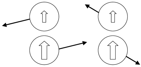
Figure 1: Paired fermions 1 and 2 (left), and 3 and 4 (right).

The usual definition of a Cooper pair is that the momenta must be equal and opposite, ${\bf p}_{1}=-{\bf p}_{2}$, and also the spins, $s_{1}=-s_{2}$.Cooper56 This is widely accepted to act as a zero momentum, zero spin effective boson. The more general definition that will be used here likewise insists that the two fermions have equal and opposite momenta, ${\bf p}_{1}=-{\bf p}_{2}$. But for the the spins it is only necessary that $s_{1}\neq s_{2}$ in order to prevent internal permutations within the Cooper pair, which would cancel the bosonic ones. For the case of electrons, which are spin-half fermions, the condition $s_{1}\neq s_{2}$ is equivalent to $s_{1}=-s_{2}$. Electrons of course are the main focus in superconductivity, in which case there is no difference in the two formulations of Cooper pairs. The more general pair may be called an effective spin-$s_{1}s_{2}$ boson, with the convention $s_{1}<s_{2}$. The total spin $s_{1}+s_{2}$ is not sufficient to label the pair. There are $S(2S+1)$ distinct species of pairs.

Consider four fermions in two pairs: $\{1,2\}$ and $\{3,4\}$ (see Fig. 1). That is, ${\bf p}_{1}=-{\bf p}_{2}$ and ${\bf p}_{3}=-{\bf p}_{4}$. Suppose that $s_{1}=s_{3}$ and $s_{2}=s_{4}$. Then the only permutations permitted are between 1 and 3 and between 2 and 4. Hence the symmetrization functionAttard18 ; Attard21 for these four fermions is

$$\sum_{\hat{\mathrm{P}}}(-1)^{p}e^{-{\bf q}\cdot[{\bf p}-{\bf p}^{\prime}]/\mathrm{i}\hbar}\delta_{{\bf s}^{\prime},{\bf s}}$$ (2.8)

$$= 1-e^{-{\bf q}_{13}\cdot{\bf p}_{13}/\mathrm{i}\hbar}-e^{-{\bf q}_{24}\cdot{\bf p}_{24}/\mathrm{i}\hbar}$$

$$\mbox{ }+e^{-{\bf q}_{13}\cdot{\bf p}_{13}/\mathrm{i}\hbar}e^{-{\bf q}_{24}\cdot{\bf p}_{24}/\mathrm{i}\hbar}$$

$$\approx 1+e^{-{\bf q}_{12}\cdot{\bf p}_{13}/\mathrm{i}\hbar}e^{-{\bf q}_{34}\cdot{\bf p}_{31}/\mathrm{i}\hbar}.$$

The prime indicates the permuted eigenvalues. The single transposition fermionic terms have been neglected in the final equality because of their rapid fluctuation compared to the retained terms, which are bosonic. The double transposition has exponent that in part is

$${\bf q}_{13}\cdot{\bf p}_{13}+{\bf q}_{24}\cdot{\bf p}_{24}$$ (2.9)

$$= \frac{1}{2}\big{[}({\bf q}_{1}+{\bf q}_{2})-({\bf q}_{3}+{\bf q}_{4})\big{]}\cdot{\bf p}_{13}$$

$$\mbox{ }+\frac{1}{2}\big{[}({\bf q}_{1}-{\bf q}_{2})-({\bf q}_{3}-{\bf q}_{4})\big{]}\cdot{\bf p}_{13}$$

$$\mbox{ }+\frac{1}{2}\big{[}({\bf q}_{1}+{\bf q}_{2})-({\bf q}_{3}+{\bf q}_{4})\big{]}\cdot{\bf p}_{24}$$

$$\mbox{ }-\frac{1}{2}\big{[}({\bf q}_{1}-{\bf q}_{2})-({\bf q}_{3}-{\bf q}_{4})\big{]}\cdot{\bf p}_{24}$$

$$= {\bf Q}_{13}\cdot{\bf P}_{13}+\frac{1}{2}({\bf q}_{12}-{\bf q}_{34})\cdot({\bf p}_{13}-{\bf p}_{24})$$

$$= {\bf q}_{12}\cdot{\bf p}_{13}+{\bf q}_{34}\cdot{\bf p}_{31}.$$

The first two equalities hold in general; the final equality holds for the Cooper pairs. The center of mass separation is ${\bf Q}_{13}={\bf Q}_{1}-{\bf Q}_{3}=({\bf q}_{1}+{\bf q}_{2})/2-({\bf q}_{3}+{\bf q}_{4})/2$, the total momentum difference is ${\bf P}_{13}=({\bf p}_{1}+{\bf p}_{2})-({\bf p}_{3}+{\bf p}_{4})$, and the ‘locations’ of the effective bosons are ${\bf q}_{12}={\bf q}_{1}-{\bf q}_{2}$ and ${\bf q}_{34}={\bf q}_{3}-{\bf q}_{4}$. For a Cooper pair the total momentum is identically zero, which gives the final equality.

In its final form the permutation weight is exactly the dimer symmetrization weight for two boson molecules located at ${\bf q}_{12}$ and ${\bf q}_{34}$ with momenta ${\bf p}_{1}$ and ${\bf p}_{3}$, respectively. Attard18 ; Attard21 This is a non-local expression since it depends only on the size (i.e. internal separation) of the two Cooper pairs. If there exists an attractive potential so that the size of a pair is small, then the fluctuations in this term are also small. There are infinitely more pairs of fermions with macroscopic separations $Q_{13}$ then there are with microscopic separations, and for these the fermionic terms fluctuate infinitely more rapidly than the bosonic terms. The former average to zero; the latter average close to unity. The Cooper pair formulation removes the macroscopic separation between the center of masses, ${Q}_{13}$. This is what makes the permutation of Cooper pairs non-local and creates the analogy with Bose-Einstein condensation and superfluidity. Attard21 ; Attard22a

II.2.2 Pair Weight for Bound Cooper Pairs

One can demonstrate the idea that a Cooper pair is an effective boson molecule by performing the classical momentum integral for the four fermions comprising the above pair dimer. The momentum integral is

$$I_{4} \equiv \Delta_{p}^{-6}\int\mathrm{d}{\bf p}^{4}\;\delta({\bf p}_{1}+{\bf p}_{2})\,\delta({\bf p}_{3}+{\bf p}_{4})\,$$

$$\mbox{ }\times e^{-\beta{\cal K}({\bf p}^{4})}e^{-{\bf q}_{12}\cdot{\bf p}_{13}/\mathrm{i}\hbar}e^{-{\bf q}_{34}\cdot{\bf p}_{31}/\mathrm{i}\hbar}$$

$$= \Delta_{p}^{-6}\int\mathrm{d}{\bf p}_{1}\,\mathrm{d}{\bf p}_{3}\;e^{-2\beta p_{1}^{2}/2m}e^{-2\beta p_{3}^{2}/2m}$$

$$\mbox{ }\times e^{-[{\bf q}_{12}-{\bf q}_{34}]\cdot{\bf p}_{1}/\mathrm{i}\hbar}e^{-[{\bf q}_{34}-{\bf q}_{12}]\cdot{\bf p}_{3}/\mathrm{i}\hbar}$$

$$= \left\{2^{-3/2}V\Lambda^{-3}e^{-\pi[{\bf q}_{12}-{\bf q}_{34}]^{2}/2\Lambda^{2}}\right\}^{2}$$

$$\approx 2^{-3/2}V\Lambda^{-3}\frac{\Lambda e^{-\pi q_{12}^{2}/\Lambda^{2}}}{q_{12}\sqrt{2\pi}}\sinh^{1/2}(2\pi q_{12}^{2}/\Lambda^{2})$$

$$\mbox{ }\times 2^{-3/2}V\Lambda^{-3}\frac{\Lambda e^{-\pi q_{34}^{2}/\Lambda^{2}}}{q_{34}\sqrt{2\pi}}\sinh^{1/2}(2\pi q_{34}^{2}/\Lambda^{2}).$$

Since the permutations of Cooper pairs are non-local, the vast majority are at macroscopic separations and are therefore uncorrelated. The final equality follows by averaging the coupling exponential over the alignment angle,

$$\frac{1}{2}\int_{-1}^{1}\mathrm{d}x\;e^{2\pi q_{12}q_{34}x/\Lambda^{2}}$$ (2.11)

$$= \frac{\Lambda^{2}}{2\pi q_{12}q_{34}}\sinh\!\big{(}\frac{2\pi q_{12}q_{34}}{\Lambda^{2}}\big{)}$$

$$\approx \frac{\Lambda}{q_{12}\sqrt{2\pi}}\sinh^{1/2}(2\pi q_{12}^{2}/\Lambda^{2})$$

$$\mbox{ }\times\frac{\Lambda}{q_{34}\sqrt{2\pi}}\sinh^{1/2}(2\pi q_{34}^{2}/\Lambda^{2}).$$

The second equality is valid if $q_{12}\approx q_{34}$, which is the case when the pairs are bound at the minimum in the pair potential of mean force $\overline{q}$.

In this formulation the weight of the pair dimer factorizes into the product of weights of each pair. A mean field approximation (fix the neighbors in the most likely parallel configuration and average the intervening pair successively around the permutation loop) shows that a similar factorization holds for the pair trimer, etc. Therefore each Cooper pair is a boson molecule with average internal weight due to the transposition

$$\nu_{\mathrm{mf}} \equiv \left\langle e^{-\pi q_{12}^{2}/\Lambda^{2}}\frac{\Lambda}{q_{12}\sqrt{2\pi}}\sinh^{1/2}(2\pi q_{12}^{2}/\Lambda^{2})\right\rangle_{\mathrm{bnd}}$$ (2.12)

$$\approx \frac{\Lambda e^{-\pi\overline{q}^{2}/\Lambda^{2}}}{\overline{q}\sqrt{2\pi}}\sinh^{1/2}(2\pi\overline{q}^{2}/\Lambda^{2}).$$

This holds for a bound Cooper pair in which the pair potential of mean force has a relatively narrow minimum at $\overline{q}$. This expression for the internal weight for the bound Cooper pair effective boson is less than unity; the expression itself is likely an overestimate due to the mean field approximation (see the Appendix). The internal weight goes to zero as the size of Cooper pair goes to infinity. The remaining factor of $2^{-3/2}\Lambda^{-3}V$ from the momentum integral holds for all Cooper pairs and will be included explicitly below.

The factorization is valid if the sizes of the bound Cooper pairs are all at the minimum of the pair potential of mean force $\overline{q}$. This means that the departure from the minimum $\Delta_{q}$ must be small,

$$\Delta_{q}\ll\overline{q}/2\mbox{ and }\Delta_{q}\overline{q}\ll\Lambda^{2}/2.$$ (2.13)

This is the case if the curvature of the pair potential of mean force is large enough, $\beta\overline{w}^{\prime\prime}\Delta_{q}^{2}/2\gg 1$. This is necessary for the existence of bound Cooper pairs.

II.2.3 Number of Bound Cooper Pairs

Distinguish between Cooper pairs and bound Cooper pairs, the latter being separated by less than $\overline{q}+\Delta_{q}$. There are $N_{0,s^{\prime}s^{\prime\prime}}$ Cooper $s^{\prime}s^{\prime\prime}$-pairs, and $N_{0,s^{\prime}s^{\prime\prime}}^{\mathrm{bnd}}$ bound Cooper $s^{\prime}s^{\prime\prime}$-pairs.

The number of bound fermion couples without regard to spin or momentum is

$$N_{\mathrm{bnd}}=\frac{\rho^{2}V}{2}v_{\mathrm{bnd}},$$ (2.14)

where the bound volume is defined as

$$v_{\mathrm{bnd}} \equiv 4\pi\int_{0}^{\overline{q}+\Delta_{q}}\mathrm{d}q\;q^{2}g(q)$$ (2.15)

$$\approx 4\pi\overline{q}^{2}e^{-\beta\overline{w}}\sqrt{2\pi/\beta\overline{w}^{\prime\prime}}.$$

This assumes that the radial distribution function, $g(q)=e^{-\beta w(q)}$, is sufficiently sharply peaked about the minimum in the pair potential of mean force to enable a second order expansion and evaluation of the Gaussian integral. Also the core exclusion region is assumed close enough to the minimum that the lower limit can be extended to zero. It is not essential to make the Gaussian approximation to the integral, since it can be evaluated numerically by fixing $\overline{q}+\Delta_{q}$ at the barrier to the potential of mean force, if it has one (see discussion in § IV). But the Gaussian results do enable a transparent analysis and a physical interpretation of the nature of the bound Cooper pairs.

The ratio of Cooper pairs to the number of fermions must be the same as the ratio of bound Cooper pairs to the number of bound fermions. Hence one must have

$$N_{0,s^{\prime}s^{\prime\prime}}^{\mathrm{bnd}}=\frac{N_{\mathrm{bnd}}}{N}N_{0,s^{\prime}s^{\prime\prime}}.$$ (2.16)

This is an important result.

II.2.4 Symmetrization Function for Cooper Pairs

The symmetrization function for Cooper pairs is dominated by the bound Cooper pairs and is

$$\eta^{+}_{0,s^{\prime}s^{\prime\prime}}\approx\nu^{N_{0,s^{\prime}s^{\prime\prime}}^{\mathrm{bnd}}}N_{0,s^{\prime}s^{\prime\prime}}^{\mathrm{bnd}}!.$$ (2.17)

The superscript + indicates that these are treated as effective bosons. The result follows because the permutations of the bound Cooper pairs are non-local and each carries the internal weight of the effective boson, $\nu$.

II.3 Grand Potential with Paired Fermions

II.3.1 Continuum Momentum Limit

In my treatment of superfluidity,Attard22a I discussed taking the continuum momentum limit by adding the discrete momentum ground state explicitly to the continuum integral over the supposedly excited momentum states. Although it appears that the continuum integral also counts the momentum ground state, it seems that the double counting has negligible effect because, at least in the case of ideal bosons, each case dominates the other in its regime of applicability.Attard22a In any case the formulation that adds the discrete momentum ground state explicitly to the continuum integral over excited states has become well established ever since it was apparently invoked by London in his original ideal boson theory of superfluidity.London38

One can perform a similar trick for Cooper pairs. For fermions 1 and 2 write the discrete sum over momentum states as

$$\sum_{{\bf p}_{1},{\bf p}_{2}} = \sum_{{\bf p}_{1}}\left\{\delta_{{\bf p}_{2},-{\bf p}_{1}}+\sum_{{\bf p}_{2}}\!^{({\bf p}_{2}\neq-{\bf p}_{1})}\right\}$$ (2.18)

$$= \sum_{{\bf p}_{1}}\left\{\delta_{{\bf p}_{2},-{\bf p}_{1}}+\Delta_{p}^{-3}\int\mathrm{d}{\bf p}_{2}\right\}$$

$$= \frac{1}{\Delta_{p}^{6}}\int\mathrm{d}{\bf p}_{1}\,\mathrm{d}{\bf p}_{2}\left\{\Delta_{p}^{3}\delta({\bf p}_{2}+{\bf p}_{1})+1\right\}.$$

In transforming to the continuum integral, I assume that the point ${\bf p}_{2}=-{\bf p}_{1}$ is a set of measure zero and so this formulation it is not really double counting. In this form the integral covers the possible states of the two fermions as both paired and unpaired. A similar procedure for the product of momentum sums for $N$ fermions leads to a binomial expansion, the terms of which consist of a certain number of paired and a certain number of unpaired fermions, as is now derived.

II.3.2 Numbers of Paired and Unpaired Fermions

Let $N_{s}$ be the total number of spin-$s$ fermions, and let $N_{1,s}$ be the number of unpaired spin-$s$ fermions. Let $N_{0,ss^{\prime}}$ be the number of paired fermions with spin pair $ss^{\prime}$. To count pairs uniquely, $s<s^{\prime}$; for convenience I define $N_{0,ss^{\prime}}=N_{0,s^{\prime}s}$ and $N_{0,ss}=0$. Obviously

$$N_{s}=N_{1,s}+\sum_{s^{\prime}=-S}^{S}N_{0,ss^{\prime}}.$$ (2.19)

Also $N=\sum_{s=-S}^{S}N_{s}$.

In the first instance take the Hamiltonian to be independent of spin, in which case $\overline{N}_{s}=N/(2S+1)$. This requirement is relaxed when a spin-dependent potential is included.

I shall treat the paired and unpaired fermions as $(S+1)(2S+1)$ different species, and only allow permutations within each species. This is is similar to the no mixing approximation that I have used in the treatment of superfluidity.Attard22a For the occupancy $\{\underline{N}_{0},\underline{N}_{1}\}\equiv\{N_{0,ss^{\prime}},N_{1,s}\}$ the total number of permutations restricted to each species is

$$M = \prod_{s=-S}^{S}N_{1,s}!\prod_{s^{\prime}=-S}^{S}\prod_{s^{\prime\prime}=s^{\prime}+1}^{S}N_{0,s^{\prime}s^{\prime\prime}}!$$ (2.20)

$$= \prod_{s,s^{\prime}<s^{\prime\prime}}N_{1,s}!\,N_{0,s^{\prime}s^{\prime\prime}}!.$$

The second equality defines the abbreviated notation that will be used. This permutation number $M$ goes directly into the denominator in conjunction with the symmetrization factor formalism for the partition function that treats the paired and unpaired fermions as different species.

One can also see this from the binomial expansion that arises from the transformation to the continuum mentioned above. The usual multinomial factor that arises in the expansion is

$$\prod_{s,s^{\prime}<s^{\prime\prime}}\frac{N_{s}!}{N_{1,s}!\,N_{0,s^{\prime}s^{\prime\prime}}!}.$$ (2.21)

Inserting this into the grand partition function, Eq. (2.6), the numerator here cancels with the denominator there, leaving $M$ as the denominator in that equation.

II.3.3 Grand Partition Function

In view of either of these two results, the grand partition function for paired and unpaired fermions is

$$\Xi^{-} = \sum_{\underline{N}_{0},\underline{N}_{1}}\frac{z^{N}}{\prod_{s,s^{\prime}<s^{\prime\prime}}N_{1,s}!\,N_{0,s^{\prime}s^{\prime\prime}}!}$$ (2.22)

$$\mbox{ }\times\sum_{\bf p}\sum_{\hat{\mathrm{P}}}(-1)^{p_{1,s}}\left\langle\phi_{\bf p}({\bf q})\left|e^{-\beta\hat{\cal H}}\right|\phi_{\bf p}\big{(}\hat{\mathrm{P}}{\bf q}\big{)}\right\rangle$$

$$\approx \sum_{\underline{N}_{0},\underline{N}_{1}}\frac{z^{N}V^{-N}}{\prod_{s,s^{\prime}<s^{\prime\prime}}N_{1,s}!\,N_{0,s^{\prime}s^{\prime\prime}}!}$$

$$\mbox{ }\times\sum_{{\bf p}}\int\mathrm{d}{\bf q}\;e^{-\beta{\cal H}({\bf q},{\bf p})}\eta^{-}({\bf q},{\bf p},{\bf s}).$$

The commutation function has been neglected in the final equality. The discrete momentum sums can be replaced directly by continuum momentum integrals since the paired and unpaired fermions have been explicitly identified. The phase space point of the $ss^{\prime}$ paired fermions is denoted ${\bf\Gamma}^{2N_{0,ss^{\prime}}}\equiv\{{\bf q}^{2N_{0,ss^{\prime}}},{\bf p}^{2N_{0,ss^{\prime}}}\}$, and the phase space point of unpaired $s$ fermions is denoted ${\bf\Gamma}^{N_{1,s}}\equiv\{{\bf q}^{N_{1,s}},{\bf p}^{N_{1,s}}\}$. The total permutator is $\hat{\mathrm{P}}=\prod_{s,s^{\prime}<s^{\prime\prime}}\hat{\mathrm{P}}_{0,s^{\prime}s^{\prime\prime}}\hat{\mathrm{P}}_{1,s}$, which factors commute.

Because permutations are confined to amongst fermions with the same spin, and because of the no mixing approximation (i.e. permutations between paired and unpaired fermions may be neglected), the symmetrization function fully factorizes

$$\eta^{-}({\bf q},{\bf p},{\bf s})=\prod_{s,s^{\prime}<s^{\prime\prime}}\eta^{+}_{0,s^{\prime}s^{\prime\prime}}({\bf\Gamma}^{2N_{0,s^{\prime}s^{\prime\prime}}})\,\eta^{-}_{1,s}({\bf\Gamma}^{N_{1,s}}).$$ (2.23)

The symmetrization function for paired fermions, $\eta_{0,s^{\prime}s^{\prime\prime}}^{+}$, was expressed above in terms of the number of bound Cooper pairs, Eq. (2.17). It is independent of the point in phase space and can be taken outside of the integrals for the partition function.

The symmetrization function for unpaired fermions is

$$\eta^{-}_{1,s}({\bf\Gamma}^{N_{1,s}})=\sum_{\hat{\mathrm{P}}_{1,s}}^{N_{1,s}!}(-1)^{p_{1,s}}e^{-[{\bf p}^{N_{1,s}}-{\bf p}^{\prime N_{1,s}}]\cdot{\bf q}^{N_{1,s}}/\mathrm{i}\hbar}.$$ (2.24)

Here ${\bf p}^{\prime N_{1,s}}\equiv\hat{\mathrm{P}}_{1,s}{\bf p}^{N_{1,s}}$, and $p_{1,s}$ is the parity of the permutation $\hat{\mathrm{P}}_{1,s}$.

In the general classical phase space formulation of quantum statistical mechanics, the permutation loop expansion, which consists of products of loops, can be written as the exponential of a series of single loops. Attard18 ; Attard21 It follows that the grand potential is the sum of loop potentials, each of which is the classical average of a sum over single permutation loops of a given size. This holds only for the unpaired fermions, whose symmetrization function has $(2S+1)$ factors. Each factor gives a corresponding loop grand potential; for $l\geq 2$ these can all be treated independently.

II.3.4 Configuration Integral Containing Bound Cooper Pairs

Shortly the monomer or classical grand potential will be given, and this depends upon the classical configurational integral containing $N^{\mathrm{bnd}}_{0}=\sum_{s^{\prime}<s^{\prime\prime}}N^{\mathrm{bnd}}_{0,s^{\prime}s^{\prime\prime}}$ bound Cooper pairs. This is different to the classical configurational integral $Q(N,V,T)$ unconstrained by such pairing. The two are related as

$$Q(N,V,T|\underline{N}^{\mathrm{bnd}}_{0})$$ (2.25)

$$= \int_{V}\mathrm{d}{\bf q}^{N_{1}}\mathrm{d}{\bf q}^{2N_{0}-N_{0}^{\mathrm{bnd}}}\int_{\Delta_{V}}\mathrm{d}{\bf q}^{N_{0}^{\mathrm{bnd}}}\;e^{-\beta U({\bf q}^{N})}$$

$$= Q(N,V,T)\left\langle\prod_{j=1}^{N_{0}^{\mathrm{bnd}}}\Theta(\overline{q}+\Delta_{q}-q_{jj^{\prime}})\right\rangle$$

$$= Q(N,V,T)\left\{\frac{1}{V}4\pi\int_{0}^{\overline{q}+\Delta_{q}}\mathrm{d}q\;q^{2}g(q)\right\}^{N_{0}^{\mathrm{bnd}}}$$

$$\equiv Q(N,V,T)\prod_{s^{\prime}<s^{\prime\prime}}\frac{v_{\mathrm{bnd}}^{N^{\mathrm{bnd}}_{0,s^{\prime}s^{\prime\prime}}}}{V^{N^{\mathrm{bnd}}_{0,s^{\prime}s^{\prime\prime}}}}.$$

Here $j^{\prime}$ is the label of the fermion bound to $j$, and $\Theta(q)$ is the Heaviside step function. The bound weighted volume $v_{\mathrm{bnd}}$ was given in Eq. (2.15), where its proportionality to the number of bound generic fermions was given, $N_{\mathrm{bnd}}=(\rho^{2}V/2)v_{\mathrm{bnd}}$.

II.3.5 Monomer Grand Potential

Finally, the monomer or classical grand potential is

$$e^{-\beta\Omega^{(1)}(z,V,T)}$$ (2.26)

$$= \Xi_{\mathrm{cl}}(z,V,T)$$

$$= \sum_{\underline{N}_{0},\underline{N}_{1}}\frac{z^{N}\prod_{s^{\prime}<s^{\prime\prime}}\nu^{N^{\mathrm{bnd}}_{0,s^{\prime}s^{\prime\prime}}}N^{\mathrm{bnd}}_{0,s^{\prime}s^{\prime\prime}}!}{V^{N}\prod_{s,s^{\prime}<s^{\prime\prime}}N_{1,s}!N_{0,s^{\prime}s^{\prime\prime}}!}$$

$$\mbox{ }\times\prod_{s,s^{\prime}<s^{\prime\prime}}\frac{\Delta_{p}^{-3N_{1,s}}}{\Delta_{p}^{3N_{0,s^{\prime}s^{\prime\prime}}}}\int\mathrm{d}{\bf p}^{N_{0,s^{\prime}s^{\prime\prime}}}\,\mathrm{d}{\bf p}^{N_{1,s}}e^{-\beta{\cal K}({\bf p}^{N})}$$

$$\mbox{ }\times\int_{V}\mathrm{d}{\bf q}^{N_{1}}\mathrm{d}{\bf q}^{N_{0}-N_{0}^{\mathrm{bnd}}}\int_{\Delta_{V}}\mathrm{d}{\bf q}^{N_{0}^{\mathrm{bnd}}}\;e^{-\beta U({\bf q}^{N})}$$

$$= \sum_{\underline{N}_{0},\underline{N}_{1}}\frac{z^{N}\prod_{s^{\prime}<s^{\prime\prime}}\nu^{N^{\mathrm{bnd}}_{0,s^{\prime}s^{\prime\prime}}}N^{\mathrm{bnd}}_{0,s^{\prime}s^{\prime\prime}}!}{V^{N}\prod_{s,s^{\prime}<s^{\prime\prime}}N_{1,s}!N_{0,s^{\prime}s^{\prime\prime}}!}$$

$$\mbox{ }\times\prod_{s,s^{\prime}<s^{\prime\prime}}\frac{(V/\Lambda^{3})^{N_{1,s}}}{(2^{3/2}\Lambda^{3}/V)^{N_{0,s^{\prime}s^{\prime\prime}}}}\,Q(N,V,T|\underline{N}^{\mathrm{bnd}}_{0})$$

$$= \sum_{\underline{N}_{0},\underline{N}_{1}}\prod_{s^{\prime}<s^{\prime\prime}}\frac{(\nu v_{\mathrm{bnd}})^{N^{\mathrm{bnd}}_{0,s^{\prime}s^{\prime\prime}}}N^{\mathrm{bnd}}_{0,s^{\prime}s^{\prime\prime}}!}{V^{N^{\mathrm{bnd}}_{0,s^{\prime}s^{\prime\prime}}}}$$

$$\mbox{ }\times\prod_{s^{\prime}<s^{\prime\prime}}\frac{V^{N_{0,s^{\prime}s^{\prime\prime}}}}{(2^{3/2}\Lambda^{3})^{N_{0,s^{\prime}s^{\prime\prime}}}N_{0,s^{\prime}s^{\prime\prime}}!}$$

$$\mbox{ }\times\prod_{s}\frac{(V/\Lambda^{3})^{N_{1,s}}}{N_{1,s}!}\times\frac{z^{N}}{V^{N}}Q(N,V,T).$$

Here the continuum momentum limit has been taken. The classical configuration integral, $Q(N,V,T)$, is independent of the spin state of the fermions (unless a spin-dependent potential is added). As above, $N=\sum_{s}N_{1,s}+\sum_{s^{\prime}<s^{\prime\prime}}N_{0,s^{\prime}s^{\prime\prime}}$.

II.3.6 Unpaired Grand Potential

For unpaired fermions the loop grand potential is straightforward to derive as, apart from a factor of $(-1)^{l-1}$, it is identical to that for bosons. Attard18 ; Attard21 The unpaired loop grand potentials $l\geq 2$ are classical averages (§5.3 of Ref. Attard21, ), which can be taken canonically

$$-\beta\Omega^{-,(l)}_{1,s} = \left\langle\eta^{-,(l)}_{1,s}({\bf p}^{N_{s}},{\bf q}^{N_{s}})\right\rangle_{\underline{N}_{0},\underline{N}_{1}}^{\mathrm{cl}}$$ (2.27)

$$= (-1)^{l-1}\left\langle G^{(l)}({\bf q}^{N_{1,s}})\right\rangle_{\underline{N}_{0},\underline{N}_{1}}^{\mathrm{cl}}$$

$$= (-1)^{l-1}\left(\frac{N_{1,s}}{N}\right)^{l}\left\langle G^{(l)}({\bf q}^{N})\right\rangle_{N}^{\mathrm{cl}}$$

$$\equiv N_{1,s}(-1)^{l-1}\left(\frac{N_{1,s}}{N}\right)^{l-1}g^{(l)}.$$

The fermionic anti-symmetrization factor $(-1)^{l-1}$ appears explicitly. Apart from it, all factors are positive. The average has been transformed from the mixed $\{\underline{N}_{0},\underline{N}_{1}\}$ system to the classical configurational system of $N$ fermions that does not distinguish their state.Attard21 The factor of $\left({N_{s,1}}/{N}\right)^{l}$ is the uncorrelated probability that $l$ fermions chosen at random in the original mixed system are all unpaired and in the same state. The Gaussian position loop function is

$$G^{(l)}({\bf q}^{N})=\sum_{j_{1},\ldots,j_{l}}^{N}{}^{\prime\prime}\hskip 2.84544pte^{-\pi q_{j_{l},j_{1}}^{2}/\Lambda^{2}}\prod_{k=1}^{l-1}e^{-\pi q_{j_{k},j_{k+1}}^{2}/\Lambda^{2}}.$$ (2.28)

The double prime indicates that no two indeces may be equal and that distinct loops must be counted once only. There are $N!/(N-l)!l$ distinct $l$-loops here, the overwhelming number of which are negligible upon averaging. Since the pure excited momentum state permutation loops are compact in configuration space, one can define an intensive form of the average loop Gaussian, $g^{(l)}\equiv\left\langle G^{(l)}({\bf q}^{N})\right\rangle_{N}^{\mathrm{cl}}/N$. This is convenient because it does not depend upon $N_{1,s}$.

II.4 Maximum Entropy for Paired Fermions

The constrained grand potential is given by

$$-\beta\Omega^{-}(\underline{N}_{0},\underline{N}_{1}|z,V,T)$$

$$= -\beta\Omega^{(1)}(\underline{N}_{0},\underline{N}_{1}|z,V,T)-\beta\sum_{s=-S}^{S}\sum_{l=2}^{\infty}\Omega^{-,(l)}_{1,s}(\underline{N}_{0},\underline{N}_{1}).$$

The monomer and paired loop potentials on the right hand side are given above.

This is the constrained total entropy and the optimum number of paired and unpaired fermions is determined by maximizing it. It is most convenient to take the derivatives at constant number $N$.

In the absence of a spin-dependent potential, all spins are equal, $N_{s}=N/(2S+1)$. Similarly the pair number is independent of the spin pair $s^{\prime}s^{\prime\prime}$, $N_{0,s^{\prime}s^{\prime\prime}}=[1-\delta_{s^{\prime},s^{\prime\prime}}]\tilde{N}_{0}$, so that $N_{s}=N_{1,s}+\sum_{s^{\prime}}N_{0,ss^{\prime}}=N_{1,s}+2S\tilde{N}_{0}$. One can ensure the derivative at constant $N$ by taking $\mathrm{d}N_{1,s^{\prime}}=\mathrm{d}N_{1,s^{\prime\prime}}=-\mathrm{d}N_{0,s^{\prime}s^{\prime\prime}}$. Setting $N_{1,s^{\prime}}=N_{1,s^{\prime\prime}}$ after the differentiation one has

$$\frac{\mathrm{d}(-\beta\Omega)}{\mathrm{d}N_{1,s^{\prime}}} = \ln\frac{VN_{0,s^{\prime}s^{\prime\prime}}}{2^{-3/2}\Lambda^{3}N_{1,s^{\prime}}^{2}}-\frac{N_{\mathrm{bnd}}}{N}\ln\frac{\nu v_{\mathrm{bnd}}N_{\mathrm{bnd}}N_{0,s^{\prime}s^{\prime\prime}}}{NV}$$ (2.30)

$$\mbox{ }+2\sum_{l=2}^{\infty}(-1)^{l-1}l\frac{N_{1,s^{\prime}}^{l-1}}{N^{l-1}}g^{(l)}.$$

Substituting $N_{0,s^{\prime}s^{\prime\prime}}=(N_{s^{\prime}}-N_{1,s^{\prime}})/2S$ and setting the derivative to zero determines $\overline{N}_{1,s^{\prime}}$ for fixed $N$ and $V$. If the right hand side is positive, then $N_{1,s^{\prime}}$ should be increased.

At high temperatures, the intensive Gaussian loop integrals are negligible, $g^{(l)}\approx 0$, as are the number of bound generic pairs, $N_{\mathrm{bnd}}$. In this regime the solution corresponds to the argument of the first logarithm being unity, or

$$\overline{N}_{0,s^{\prime}s^{\prime\prime}}=2^{-3/2}\Lambda^{3}\overline{\rho}_{1,s^{\prime}}\,\overline{N}_{1,s^{\prime}}.$$ (2.31)

One sees that the number of Cooper pairs is relatively negligible until the temperature is low enough that $\rho\Lambda^{3}\gtrsim 2^{3/2}$ (assuming that the intensive Gaussian loop integrals remain negligible).

II.4.1 Spin Dependent External Potential

Add an external spin-dependent one-body potential, $U(\sigma)=-B\sum_{j}\sigma_{j}$. Assume that there is no pair or many-body potential that depends upon the spins. The classical configuration integral becomes

$$Q(N,V,T,B) = \prod_{s,s^{\prime}<s^{\prime\prime}}e^{s\beta BN_{1,s}}e^{(s^{\prime}+s^{\prime\prime})\beta BN_{0,s^{\prime}s^{\prime\prime}}}$$ (2.32)

$$\mbox{ }\times Q(N,V,T).$$

To the monomer grand potential $-\beta\Omega^{(1)}$ should be added

$$\beta B\sum_{s}sN_{1,s}+\beta B\sum_{s^{\prime}<s^{\prime\prime}}(s^{\prime}+s^{\prime\prime})N_{0,s^{\prime}s^{\prime\prime}}.$$ (2.33)

In general the derivatives are messy because the $N_{1,s}$ and $N_{0,s^{\prime}s^{\prime\prime}}$ vary with spin. But for electrons, $S=1/2$, one can carry out the derivatives at constant $N$ in two ways to give two equations for two unknowns. The first way is to take $\mathrm{d}N_{1,\uparrow}=\mathrm{d}N_{1,\downarrow}=-\mathrm{d}N_{0,\uparrow\downarrow}$. This gives

$$\frac{\mathrm{d}(-\beta\Omega)}{\mathrm{d}N_{1,\uparrow}} = \ln\frac{V}{\Lambda^{3}N_{1,\uparrow}}+\ln\frac{V}{\Lambda^{3}N_{1,\downarrow}}-\ln\frac{2^{-3/2}\Lambda^{-3}V}{N_{0,\uparrow\downarrow}}$$ (2.34)

$$\mbox{ }-\frac{N_{\mathrm{bnd}}}{N}\ln\frac{\nu v_{\mathrm{bnd}}N_{\mathrm{bnd}}N_{0,\uparrow\downarrow}}{NV}$$

$$\mbox{ }+\sum_{l=2}^{\infty}(-1)^{l-1}l\frac{N_{1,\uparrow}^{l-1}+N_{1,\downarrow}^{l-1}}{N^{l-1}}g^{(l)}.$$

The second way is to take $\mathrm{d}N_{1,\uparrow}=-\mathrm{d}N_{1,\downarrow}$ and $\mathrm{d}N_{0,\uparrow\downarrow}=0$, which gives

$$\frac{\mathrm{d}(-\beta\Omega)}{\mathrm{d}N_{1,\uparrow}} = \ln\frac{V}{\Lambda^{3}N_{1,\uparrow}}-\ln\frac{V}{\Lambda^{3}N_{1,\downarrow}}+\beta B$$

$$\mbox{ }+\sum_{l=2}^{\infty}(-1)^{l-1}l\frac{N_{1,\uparrow}^{l-1}-N_{1,\downarrow}^{l-1}}{N^{l-1}}g^{(l)}.$$

The number of paired electrons can be eliminated from these by writing $N_{0,\uparrow\downarrow}=[N-N_{1,\uparrow}-N_{1,\downarrow}]/2$.

III Results

Table 1: Intensive loop Gaussian for saturated liquid Lennard-Jones He³ at various temperatures, $T^{*}\equiv k_{\mathrm{B}}T/\varepsilon$.

$T^{*}$	$g^{(2)}$	$g^{(3)}$	$g^{(4)}$	$g^{(5)}$
1.2	5.43E-03	2.22E-04	1.67E-05	1.77E-06
1.1	1.11E-02	7.84E-04	9.69E-05	1.60E-05
1.0	2.09E-02	2.40E-03	4.58E-04	1.14E-04
0.9	3.80E-02	6.85E-03	1.92E-03	6.93E-04
0.8	6.99E-02	2.00E-02	8.47E-03	4.64E-03
0.7	1.27E-01	5.73E-02	3.65E-02	2.97E-02
0.6	2.31E-01	1.64E-01	1.59E-01	1.94E-01

Table 1 gives the intensive loop Gaussians for Lennard-Jones helium-3. The Lennard-Jones parameters model helium, $\varepsilon_{\mathrm{He}}=10.22k_{\mathrm{B}}$ J and $\sigma_{\mathrm{He}}=0.2556$ nm.Sciver12 The Monte Carlo simulation algorithm used to obtain the results is detailed in Ch. 5 of Ref. Attard21, . In general the loop Gaussians increase with decreasing temperature. They also decrease with increasing loop size, except at the lowest temperature studied. This suggests that terminating the loop series with $l^{\mathrm{max}}=5$ at these temperatures will give reliable results since each term is weighted by the corresponding power of $N_{1,s}/N\leq 1/(2S+1)$.

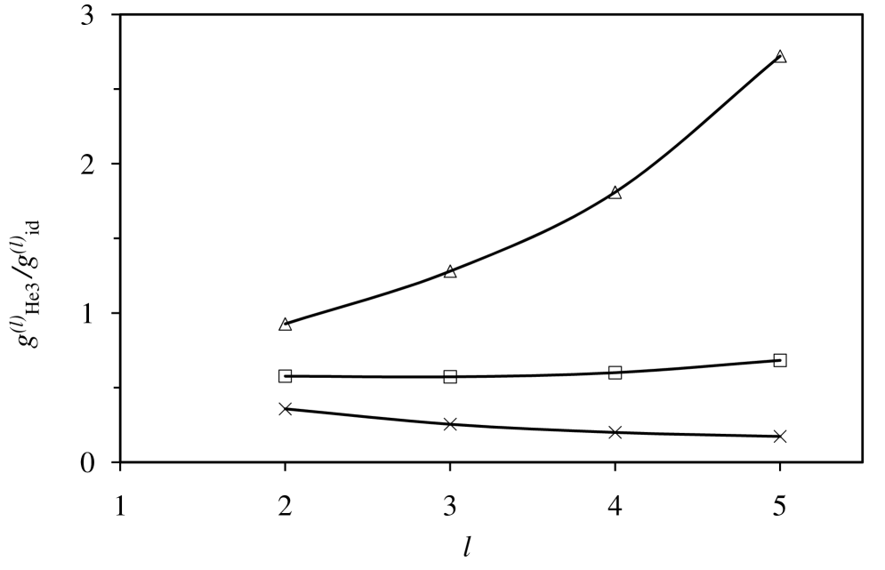
Figure 2: Ratio of intensive loop Gaussian $g^{(l)}$ for Lennard-Jones ³He to that for ideal fermions at Lennard-Jones helium saturation liquid densities. The triangles are for $\rho\Lambda^{3}=1.4$ ($T^{*}=0.6$), the squares are for $\rho\Lambda^{3}=1.2$ ($T^{*}=0.7$), and the crosses are for $\rho\Lambda^{3}=1.1$ ($T^{*}=0.8$). Note $T[\mathrm{K}]=10.22T^{*}$.

Figure 2 compares the intensive loop Gaussians $g^{(l)}$ for Lennard-Jones ³He and for ideal fermions by plotting their ratio for three temperatures. The intensive loop Gaussian for ideal particles, derived in §4.1 of Ref. Attard21, , is

$$g^{(l)}_{\mathrm{id}} = \frac{1}{N}\left\langle G^{(l)}({\bf q}^{N})\right\rangle_{N,\mathrm{cl,id}}$$ (3.1)

$$= \frac{1}{N}\frac{N!}{(N-l)!l}\frac{1}{V^{l}}\int\,\mathrm{d}{\bf q}^{l}\;e^{-\pi q_{l,1}^{2}/\Lambda^{2}}\prod_{k=1}^{l-1}e^{-\pi q_{k,{k+1}}^{2}/\Lambda^{2}}$$

$$= \frac{\rho^{l-1}}{l}\Lambda^{3(l-1)}l^{-3/2}.$$

It can be seen that at the lowest temperature, the intensive loop Gaussians the Lennard-Jones model is larger than that for ideal fermions, increasingly so as the order of the loop increases. The presence of an attractive potential of mean force strongly affects the particle correlation functions and hence the values of the intensive loop Gaussians that determine the number of Cooper pairs.

Table 2: Parameters for saturated liquid Lennard-Jones He³ at various temperatures, $T^{*}\equiv k_{\mathrm{B}}T/\varepsilon$. The Lennard-Jones diameter $\sigma$ is the unit of length.

$T^{*}$	1.2	1.1	1.0	0.9	0.8	0.7	0.6
$\rho$	0.53	0.63	0.70	0.75	0.80	0.85	0.89
$\Lambda$	1.13	1.18	1.23	1.30	1.38	1.47	1.59
$\rho\Lambda^{3}$	0.59	0.74	0.86	0.98	1.11	1.25	1.41
$\overline{q}$	1.100	1.097	1.093	1.091	1.090	1.089	1.088
$\beta\overline{w}$	$-0.74$	$-0.81$	$-0.88$	$-0.95$	$-1.03$	$-1.12$	$-1.20$
$\beta\overline{w}^{\prime\prime}$	64.49	87.17	87.39	100.78	135.60	151.93	176.07
$\nu$	0.32	0.33	0.35	0.37	0.39	0.42	0.45
$v_{\mathrm{bnd}}$	9.92	9.12	9.68	9.63	9.03	9.25	9.38
$\frac{4\pi\overline{q}}{\Lambda^{2}\sqrt{\beta\overline{w}^{\prime\prime}}}$	1.36	1.07	0.97	0.81	0.62	0.51	0.41

Table 2 gives the values of various parameters obtained by classical canonical simulations of 5,000 Lennard-Jones helium-3 atoms in a homogeneous system with periodic boundary conditions. The density is the liquid saturation density, which was obtained along the saturation curve for a liquid drop. It can be seen that the minimum in the pair potential of mean force gets deeper, and its curvature increases, with decreasing temperature. The internal weight $\nu$ and the bound volume $v_{\mathrm{bnd}}$ are surprisingly insensitive to temperature. The parameter ${4\pi\overline{q}}/{\Lambda^{2}\sqrt{\beta\overline{w}^{\prime\prime}}}$ should be much less than unity for the present numerical approximations to be valid. The relation between the Lennard-Jones dimensionless temperature and the actual temperature is $T[\mathrm{K}]=10.22T^{*}$.

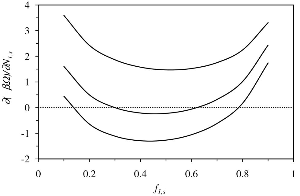
Figure 3: Entropy derivative as a function of fraction of unpaired fermions for Lennard-Jones ³He, $S=1/2$, at various temperatures along the Lennard-Jones saturation liquid curve at $B=0$. From bottom to top the curves are $T^{*}=$ 0.9, 1.0, and 1.1. The dotted line is a guide to the eye. Intensive loop Gaussians up to $l^{\mathrm{max}}=5$ were used.

Figure 3 shows the thermodynamic force acting on the fraction of unpaired fermions, with positive values driving an increase. The curves that don’t pass thorough zero have a positive derivative for the whole domain, which means that the system in its optimum thermodynamic state is composed entirely of unpaired fermions.

For the curves with two zeros, one is a local maximum and the other is a local minimum in the total entropy. The stable solution, the local maximum, is the one with the smaller fraction of unpaired fermions. Integration of these approximate parabolas shows that the total entropy is approximately a cubic. At the highest temperature shown the total entropy is monotonic increasing with increasing unpaired fraction. With the emergence of distinct extrema from the point of inflection slightly above the middle temperature shown, $T^{*}=1.0$, the entropy must first decrease for the system to get from the unpaired state $f_{1,s}=1$ to the local entropy maximum at $f_{1,s}\approx 0.3$. In other words, there is a thermodynamic barrier to the formation of paired fermions. This means that the first appearance of a local entropy maximum at non-zero paired fermion fraction cannot be equated to the condensation transition. nb1

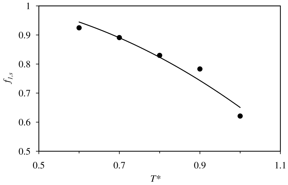
Figure 4: Fraction of unpaired fermions at the local entropy minimum for saturated liquid Lennard-Jones ³He, $S=1/2$, as a function of temperature. The curve is a quadratic best fit constrained to pass through $f_{1,s}=1$ at $T^{*}=0$.

The fraction of unpaired ³He fermions at the entropy minimum, Fig. 4, increases with decreasing temperature. The quadratic fit shows that the data is not incompatible with an entropy minimum in the fully unpaired system at $T=0$. When the entropy minimum reaches $f_{1,s}=1$, there is no longer a barrier to the entropy maximum, and the condensation transition occurs. The measured condensation transition in ³He occurs at $2.491$ mK on the melting curve.Wiki

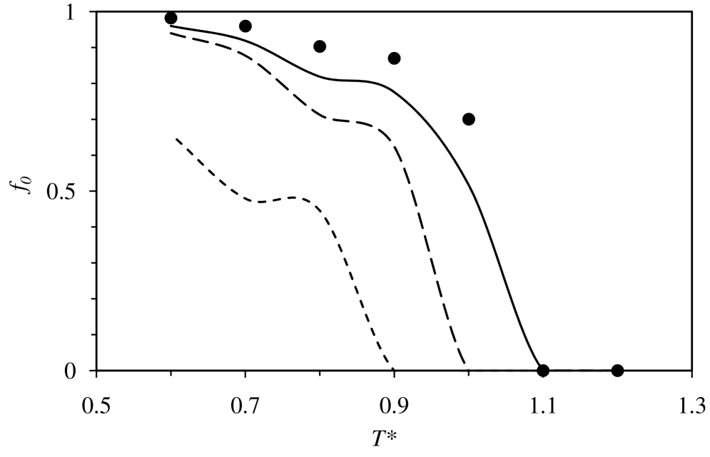
Figure 5: Fraction of paired fermions at the local entropy maximum for saturated liquid Lennard-Jones ³He, $S=1/2$, as a function of temperature. The circles are for $B=0$, the solid curve is for $\beta B=1$, the long dashed curve is for $\beta B=2$, and the short dashed curve is for $\beta B=5$.

Figure 5 shows the fraction of paired ³He fermions at the local entropy maximum as a function of temperature. It can be seen that in the absence of a spin dependent potential, $B=0$, this is discontinuous at about $T^{*}\approx 1.05$, or $T=10.7$ K. As just mentioned, this cannot be interpreted as the condensation transition.

Figure 5 also shows the effect of an external spin-dependent potential, which can be thought of as an applied magnetic field. With increasing field strength, the number of Cooper pairs is reduced, and the discontinuity temperature is shifted lower. It is unclear what would occur for $S>1/2$, or for an inhomogeneous magnetic field for $S=1/2$. These tend to align the bound Cooper pairs, either by the spin dipole or the spin quadrupole, thereby increasing the internal weight $\nu$, which would presumably enhance pairing and condensation.

IV Discussion

Its worth emphasizing that the specific behavior found here (i.e. two zeros in the entropy gradient and a thermodynamic barrier to condensation) is very much dependent on the Lennard-Jones potential and the parameters for ³He. One can isolate the essence of the grand potential derivative by focussing upon the divergent behavior at the termini of the domain,

$$\frac{\mathrm{d}(-\beta\Omega)}{\mathrm{d}N_{1,s}}\sim\ln\frac{(1-f_{1,s})^{1-\rho v_{\mathrm{bnd}}/2}}{f_{1,s}^{2}},$$ (4.1)

where $f_{1,s}$ is the fraction of unpaired fermions. The remaining terms are either constant or well behaved loop terms. As $f_{1,s}\rightarrow 0$, this is large and positive. As $f_{1,s}\rightarrow 1$, and $\rho v_{\mathrm{bnd}}/2>1$, this is also large and positive. Therefore the derivative has the parabolic shape of Fig. 3. But if $\rho v_{\mathrm{bnd}}/2<1$, then in the limit $f_{1,s}\rightarrow 1$ this is large and negative, in which case there must be one zero (or an odd number of zeros), with the one closest to $f_{1,s}=1$ being an entropy maximum. In this case there is no thermodynamic barrier to condensation. Undoubtedly the remaining logarithmic constants and loop grand potentials shift the zero, but they cannot change this qualitative behavior. Using the quadratic approximation for the potential of mean force, as in Eq. (2.15), the condensation transition criterion, $\rho v_{\mathrm{bnd}}/2<1$, is

$$2\pi\rho\overline{q}^{2}e^{-\beta\overline{w}}\sqrt{\frac{2\pi}{\beta\overline{w}^{\prime\prime}}}<1.$$ (4.2)

One sees that if the pair potential of mean force acquires a minimum that is short-ranged, shallow, and highly curved, then the condensation transition will occur.

The data in Table 2 show that a Lennard-Jones fluid cannot satisfy this criterion. Hence in this case there will always be a thermodynamic barrier to condensation, albeit one that may shift to $f_{1,s}=1$ at low temperatures, at which point it ceases to be a barrier because the fully unpaired fluid sits at the entropy minimum.

In the BCS theory of superconductivity the size of the Cooper pairs is hundreds or thousands of times larger than in the present theory. It is difficult to see the above criterion, which scales with $\overline{q}^{2}$, being satisfied by BCS theory. The two theories appear qualitatively different and likely apply in different regimes. The fact that BCS theory is a quantum mechanical rather than a quantum statistical mechanical theory is consistent with it applying quantitatively to low temperature superconductors.

The present quantum statistical theory likely applies to high temperature superconductors. The condensation criterion of a short-ranged, shallow, and highly curved minimum describes the pair potential of mean force following the monotonic-oscillatory transition in a highly coupled charged system (see Fig. 1 of Ref. Attard22b, ), which provides additional evidence that this transition is responsible for high temperature superconductivity.Attard22b

The present calculations have several quantitative limitations. Obviously the Lennard-Jones pair potential is a crude approximation to the actual interactions in helium. It is likely inaccurate for low temperature, high density condensed matter because it neglects the exact short range interactions and many-body contributions. Further the present analysis approximated the pair potential of mean force by a quadratic form and evaluated the Gaussian integrals analytically, which may not be necessary in a more sophisticated numerical study. Finally, the present analysis neglected the short-ranged commutation function on the grounds that Bose-Einstein condensation is dominated by non-local permutations. Although this works well for bosons, the present results for fermions show the essential role played by the potential of mean force in binding the Cooper pair. Since the minimum in this occurs at short ranges, where the function is rapidly varying, this approximation is questionable.

The present theory reveals the physical basis and mathematical consequences of Cooper pairing, and it shows the intimate relationship between the minimum in the pair potential of mean force and condensation. The formulation of quantum statistical mechanics in classical phase space provides a new approach to Cooper pair formation, condensation, and superconductivity.

The numerical results for Lennard-Jones ³He demonstrate that a minimum in the pair potential of mean force is not sufficient for condensation. At higher temperatures there is no entropy maximum for condensed pairs, and at lower temperatures there is a thermodynamic barrier between the local entropy maximum for condensed pairs and the unpaired state. The data is consistent with the barrier disappearing close to absolute zero.

More generally the behavior of the constrained total entropy with fraction of unpaired fermions is very much dependent on the details of the pair potential of mean force. A system can go from having a thermodynamic barrier to condensation to having no barrier to condensation if the pair potential of mean force acquires a sufficiently shallow but highly curved minimum as the temperature is decreased. This is consistent with the monotonic-oscillatory transition in charge systems at high coupling. Attard22b

There are many similarities between superconductivity and my previous treatment of superfluidity.Attard22a Ultimately both phenomena are a manifestation of Bose-Einstein condensation, with the paired fermions in the present case being effective bosons. For bosons, condensation into the momentum ground state and the consequent superfluidity is driven by the increase in permutation entropy due to the non-local correlations of the momentum ground state. For paired fermions, the permutations between the zero-momentum pairs are similarly non-local. Superfluidity in a bosonic fluid persists because momentum changing collisions can only occur for the state as a whole, and hence they have to be of macroscopic, not of molecular, size. Similarly for superconductivity, because the zero momentum pairs occupy a single state. In both cases it is the permutation entropy that ensures flow without dissipation.

Appendix A Internal Weight

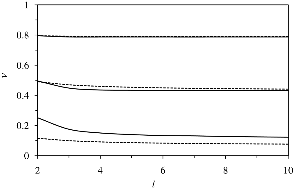
Figure 6: Internal weight per bound Cooper pair of size $\overline{q}$ as a function of permutation loop length for $z\equiv\sqrt{\pi}\,\overline{q}/\Lambda=$ 0.5 (top), 1.0 (middle) and 2.0 (bottom). The solid curves are the exact numerical result, and the dashed curves are the small $z$ asymptote. The mean field value is the exact value at $l=2$.

Figure 6 shows that the exact internal weight for a bound Cooper pair of size $\overline{q}$ decreases slowly with increasing loop size from the mean field result, Eq. (2.12), which is the exact result at $l=2$. It appears to reach a plateau for large loop size, which value would dominate the symmetrization function. This plateau is confirmed by the exact asymptotic expression,

$$\nu=e^{-z^{2}}\left\{1+\frac{l+2}{6l}z^{4}+{\cal O}(z^{8})\right\},\;\;z\rightarrow 0,$$ (A.1)

where $z\equiv\sqrt{\pi}\,\overline{q}/\Lambda$. Small $z$ is the relevant regime for Cooper pair condensation and superconductivity.

References

- (1) J. Bardeen, L. N. Cooper, and J. R. Schrieffer, “Theory of Superconductivity”, Phys. Rev. 108, 1175 (1957).
- (2) L. N. Cooper, “Bound Electron Pairs in a Degenerate Fermi Gas”, Phys. Rev. 104, 1189 (1956).
- (3) E. Maxwell, “Isotope Effect in the Superconductivity of Mercury”, Phys. Rev. 78, 477 (1950).
- (4) C. A. Reynolds, B. Serin, W. H. Wright, and L. B. Nesbitt, “Superconductivity of Isotopes of Mercury”, Phys. Rev. 78, 487 (1950).
- (5) J. G. Bednorz and K. A. Möller, “Possible high superconductivity in the Ba-La-Cu-O system”, Z. Phys. B 64, 189 (1986).
- (6) M. K. Wu, J. R. Ashburn, C. J. Torng, P. H. Hor, R. L. Meng, L. Gao, Z. J. Huang, Y. Q. Wang, and C. W. Chu, “Superconductivity at 93 K in a New Mixed-Phase Y-Ba-Cu-O Compound System at Ambient Pressure”, Phys. Rev. Lett. 58, 908 (1987).
- (7) P. Anderson, “The resonating valence bond state in La2CuO4 and superconductivity”, Science 235, 1196 (1987).
- (8) N. E. Bickers, D. J. Scalapino, and R. T. Scalettar, “CDW and SDW mediated pairing interactions”, Int. J. Mod. Phys. B 1, 687 (1987).
- (9) M. Inui, S. Doniach, P. J. Hirschfeld, A. E. Ruckenstein, Z. Zhao, Q. Yang, Y. Ni, and G. Liu, “Coexistence of antiferromagnetism and superconductivity in a mean-field theory of high-Tc superconductors”, Phys. Rev. B 37, 5182 (1988).
- (10) C. Gros, D. Poilblanc, T. M. Rice, and F. C. Zhang, “Superconductivity in correlated wavefunctions”, Physica C, 153–155, 543 (1988).
- (11) G. Kotliar, and J. Liu, “Superexchange mechanism and d-wave superconductivity”, Phys. Rev. B 38, 5142 (1988).
- (12) A. Mann. “High-temperature superconductivity at 25: Still in suspense”, Nature 475, 280 (2011).
- (13) P. Monthoux, A. V. Balatsky, and D. Pines, “Toward a theory of high-temperature superconductivity in the antiferromagnetically correlated cuprate oxides”, Phys. Rev. Lett. 67, 3448 (1991).
- (14) P. Attard, “Attraction Between Electron Pairs in High Temperature Superconductors”, arXiv:2203.02598 (2022).
- (15) P. Attard, “Quantum Statistical Mechanics in Classical Phase Space. Expressions for the Multi-Particle Density, the Average Energy, and the Virial Pressure”, arXiv:1811.00730 (2018).
- (16) P. Attard, Quantum Statistical Mechanics in Classical Phase Space, (IOP Publishing, Bristol, 2021).
- (17) P. Attard, “Bose-Einstein Condensation, the Lambda Transition, and Superfluidity for Interacting Bosons”, arXiv:2201.07382 (2022).
- (18) A. Messiah Quantum Mechanics (Vol 1 and 2) (North-Holland, Amsterdam, 1961).
- (19) E. Merzbacher, Quantum Mechanics 2nd edn (Wiley, New York, 1970).
- (20) F. London, “The -phenomenon of liquid helium and the Bose-Einstein degeneracy”, Nature 141, 643 (1938).
- (21) R. K. Pathria, Statistical Mechanics (Pergamon Press, Oxford, 1972).
- (22) S. W. van Sciver Helium Cryogenics 2nd edn (Springer, New York, 2012).
- (23) The superfluid transition in 4He shows a similar entropy minimum for small mixed loops, which thermodynamic barrier disappears for mixed loops with .Attard22a
- (24) “Helium-3”, https://en.wikipedia.org/wiki/Helium-3 Accessed 16 March 2022.