Pattern recovery by SLOPE

Abstract

SLOPE is a popular method for dimensionality reduction in the high-dimensional regression. Indeed some regression coefficient estimates of SLOPE can be null (sparsity) or can be equal in absolute value (clustering). Consequently, SLOPE may eliminate irrelevant predictors and may identify groups of predictors having the same influence on the vector of responses. The notion of SLOPE pattern allows to derive theoretical properties on sparsity and clustering by SLOPE. Specifically, the SLOPE pattern of a vector provides: the sign of its components (positive, negative or null), the clusters (indices of components equal in absolute value) and clusters ranking. In this article we give a necessary and sufficient condition for SLOPE pattern recovery of an unknown vector of regression coefficients.

[inst1]organization=Institute of Mathematics, University of Wrocław,addressline=pl. Grunwaldzki 2/4, city=Wrocław, postcode=50-384, country=Poland

[inst2]organization=Departament of Statistics, Lund University,addressline=Holger Crafoords Ekonomicentrum 1, Tycho Brahes väg 1, city=Lund, postcode=SE-220 07, country=Sweden

[inst3]organization=Institut de Mathématiques de Bourgogne, UMR 5584 CNRS, Université Bourgogne Franche-Comté,addressline=9 avenue Alain Savary, city=Dijon, postcode=21078, country=France

[inst4]organization=Laboratoire de Mathématiques LAREMA,addressline=Université d’Angers, 2 Boulevard Lavoisier, city=Angers, postcode=49045, country=France

[inst5]organization=Faculty of Mathematics and Information Science, Warsaw University of Technology,addressline=Koszykowa 75, city=Warsaw, postcode=00-662, country=Poland

[inst6]organization=Faculty of Pure and Applied Mathematics,addressline=Wrocław University of Science and Technology, Wybrzeże Wyspiańskiego 27, city=Wrocław, postcode=50-370, country=Poland

1 Introduction

High-dimensional data is currently ubiquitous in many areas of science and industry. Efficient extraction of information from such data sets often requires dimensionality reduction based on identifying the low-dimensional structure behind the data generation process. In this article we focus on a particular statistical model describing the data: the linear regression model

$${Y}={X}\beta+\varepsilon,$$ (1.1)

where $Y\in\mathbb{R}^{n}$ is a vector of responses, $X\in\mathbb{R}^{n\times p}$ is a design matrix, $\beta\in\mathbb{R}^{p}$ is an unknown vector of regression coefficients and $\varepsilon\in\mathbb{R}^{n}$ is a random noise.

It is well known that the classical least squares estimator of $\beta$ is BLUE (the best linear unbiased estimator) when the design matrix $X$ is of a full column rank. However, it is also well known that this estimator often exhibits a large variance and a large mean squared estimation error, especially when $p$ is large or when the columns of $X$ are strongly correlated. Moreover, it is not uniquely determined when $p>n$. Therefore scientists often resort to the penalized least squares estimators of the form,

$$\hat{\beta}=\operatorname*{\arg\min}_{b\in\mathbb{R}^{p}}\left[\|{Y}-{X}b\|_{2}^{2}+C\,\mathrm{pen}(b)\right],$$ (1.2)

where $C>0$ and $\mathrm{pen}$ is the penalty on the model complexity. Typical examples of the penalties include $\mathrm{pen}(\beta)=l_{0}(\beta)=\#\{i\colon\beta_{i}\neq 0\}$, which appears in popular model selection criteria such as e.g. AIC [1], BIC [2], RIC [3], mBIC [4] or EBIC [5], or the $l_{2}$ or $l_{1}$ norms, resulting in famous ridge [6, 7] or LASSO [8, 9] estimators. In case when the penalty function is not differentiable, penalized estimators usually possess the dimensionality reduction properties as illustrated e.g. in [10]. For instance, LASSO may have some null components [11, 12] and thus dimensionality reduction property of LASSO is simple: elimination of irrelevant predictors.

However, in a variety of applications one is interested not only in eliminating variables which are not important but also in merging similar values of regression coefficients. The prominent statistical example is the multiple regression with categorical variables at many levels, where one may substantially reduce the model dimension and improve the estimation and prediction properties by merging regression coefficients corresponding to ”similar” levels (see e.g. [13, 14, 15, 16, 17]). Another well known example of advantages resulting from merging different model parameters are modern Convolutional Neural Networks (CNN), where the “parameter sharing” has allowed to “dramatically lower the number of unique model parameters and to significantly increase network sizes without requiring a corresponding increase in training data” [18].

In this article we discuss the related dimensionality reduction properties of the well known convex optimization algorithm, the Sorted L-One Penalized Estimator (SLOPE) [19, 20, 21], which attracted a lot of attention due to a variety of interesting statistical properties (see, e.g., [20, 22, 23, 24] for the control of the false discovery rates under some scenarios or [25, 26, 27] for the minimax rates of the estimation and prediction errors) .

Following [19, 20] we define SLOPE as a solution to the following optimization program

$$\mbox{minimize }\left\{\frac{1}{2}\|{Y}-{X}b\|_{2}^{2}+\sum_{i=1}^{p}\lambda_{i}|b|_{(i)}\right\}\mbox{ over $b\in\mathbb{R}^{p}$},$$ (1.3)

where $|b|_{(1)}\geq|b|_{(2)}\geq\ldots\geq|b|_{(p)}$ are the absolute values of the coordinates of $b$ sorted in the nonincreasing order and the tuning parameter $\Lambda=(\lambda_{1},\ldots,\lambda_{p})^{\prime}$ satisfies $\lambda_{1}>0$ and $\lambda_{1}\geq\lambda_{2}\geq\ldots\geq\lambda_{p}\geq 0$. SLOPE is an extension of the Octagonal Shrinkage and Clustering Algorithm for Regression (OSCAR) [28] (the tuning parameter $\Lambda$ of OSCAR has arithmetically decreasing components). SLOPE is also closely related to the Pairwise Absolute Clustering and Sparsity (PACS) algorithm [29]. Concerning the above acronyms, the word “Clustering” refers to the fact that some components of OSCAR and PACS (as well as SLOPE) can be equal in absolute value. Moreover, the words “Sparsity” as well as “Shrinkage” refer to the fact that some components of these estimators can be null. SLOPE is also an extension of LASSO whose penalty term is $\lambda\|\cdot\|_{1}$ (i.e. when $\Lambda=(\lambda,\ldots,\lambda)^{\prime}$ with $\lambda>0$). Note that contrarily to SLOPE with a decreasing sequence $\Lambda$, LASSO does not exhibit clusters. Clustering and sparsity properties for both OSCAR and SLOPE are intuitively illustrated by drawing the elliptic contour lines of the residual sum of squares $b\mapsto\|Y-Xb\|_{2}^{2}$ (when $\ker(X)=\{0\}$) together with the balls of the sorted $\ell_{1}$ norm (see, e.g., Figure 2 in [28], Figure 1 in [21] or Figure 3 in [30]). Known theoretical properties include that SLOPE may cluster correlated predictors [28, 31] as well as the predictors with the similar influence on the $L_{2}$ loss function [32]. Specifically, when $X$ is orthogonal, SLOPE may also cluster components of $\beta$ equal in absolute value [33]. Therefore, dimensionality reduction properties of SLOPE are due to elimination of irrelevant predictors and grouping predictors having the same influence on $Y$. Note that contrarily to fused LASSO [34], a cluster for SLOPE does not have, in broad generality, adjacent components.

The notion of SLOPE pattern was first introduced in [35]. It allows to describe the structure (sparsity and clusters) induced by SLOPE. The SLOPE pattern extracts from a given vector:

• The sign of the components (positive, negative or null),

• The clusters (indices of components equal in absolute value),

• The hierarchy between the clusters.

Note that for a given regression model (1.1) the SLOPE pattern depends on relative scaling of different variables. In the situations where there are no clear reasons or rules for selection of specific measurement units, we suggest defining the SLOPE pattern with respect to the standardized design matrix. Note that standardizing explanatory variables is also a standard solution for a similar problem of scale dependent definition of principle components in PCA.

This article focuses on recovering the pattern of $\beta$ by SLOPE. From a mathematical perspective, the main result is Theorem 3.1, which specifies two conditions (named positivity and subdifferential conditions) characterizing pattern recovery by SLOPE. A byproduct of Theorem 3.1 is the SLOPE irrepresentability condition (IR): a necessary and sufficient condition for pattern recovery in the noiseless case. The word “irrepresentability” is a tribute to works written a decade ago on sign recovery by LASSO [36, 37, 38, 39, 40]. However, when deriving the irrepresentability condition for SLOPE we developed a substantially different mathematical framework, which paves the path for similar analyses of other penalized estimators. Furthermore, in Theorem 4.1 we consider a noisy case and under the open SLOPE irrepresentability condition (a condition slightly stronger than the SLOPE irrepresentability condition) we prove that the probability of pattern recovery by SLOPE tends to $1$ as soon as $X$ is fixed and gaps between distinct absolute values of $\beta$ diverge to infinity. Additionally, in Theorems 4.2 and 4.3 we apply the SLOPE irrepresentability condition to derive results on the asymptotic pattern recovery by SLOPE when the number of variables $p$ is fixed and the sample size $n$ diverges to infinity.

While the SLOPE ability to identify the pattern of the vector of regression coefficients $\beta$ is interesting by itself, the related reduction of model dimension brings also the advantage in terms of precision of $\beta$ estimation. This phenomenon is illustrated in Figure 1, which presents the difference in precision of LASSO and SLOPE estimators when some of the regression coefficients are equal to each other. In this example $n=100$, $p=200$, and the rows of the design matrix are generated as independent binary Markov chains, with $\mathbb{P}(X_{i1}=1)=\mathbb{P}(X_{i1}=-1)=0.5$ and $\mathbb{P}(X_{i(j+1)}\neq X_{ij})=1-\mathbb{P}(X_{i(j+1)}=X_{ij})=0.0476$. This value corresponds to the probability of the crossover event between genetic markers spaced every 5 centimorgans and our design matrix can be viewed as an example of 100 independent haplotypes, each resulting from a single meiosis event. In this example, the correlation between columns of the design matrix decays exponentially, $\rho(X_{\cdot i},X_{\cdot j})=0.9048^{|i-j|}$. The design matrix is then standardized, so that each column has a zero mean and a unit variance, and the response variable is generated according to the linear model (1.1) with $\beta_{1}=\ldots=\beta_{30}=40$, $\beta_{31}=\ldots=\beta_{200}=0$ and $\sigma=5$. In this experiment the data matrix $X$ and the regression model are constructed such that the LASSO irrepresentability condition holds. The tuning parameter for LASSO is selected as the smallest value of $\lambda$ for which LASSO can properly identify the sign of $\beta$. Similarly, the tuning parameter $\Lambda$ is designed such that the SLOPE irrepresentability condition holds and $\Lambda$ is multiplied by the smallest constant for which SLOPE properly returns the SLOPE pattern. The selected tuning parameters for LASSO and SLOPE are represented in the left panel of Figure 1. Both in case of LASSO and SLOPE, the proposed tuning parameters are close to the values minimizing the mean squared estimation error. Since in this example both LASSO and SLOPE properly estimate at $0$ null components of $\beta$, the right panel in Figure 1 illustrates only the accuracy of the estimation of the nonzero coefficients. Here we can observe that the SLOPE ability to identify the cluster structure leads to superior estimation properties. SLOPE estimates the vector of regression coefficients $\beta$ virtually without an error, while LASSO estimates are scattered over the interval between 36 and 44. In the result, the squared error of the LASSO estimator is more than 100 times larger than the squared error of SLOPE (63.4 vs 0.53).

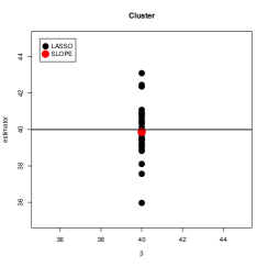
Figure 1: Comparison of LASSO and SLOPE when the cluster structure is present in the data. Here $n=100$, $p=200$, the rows of $X$ matrix are simulated as independent binary Markov chains, with the transition probability 0.0476 (corresponding to 5 centimorgans genetic distance). The correlation between $i^{th}$ and $j^{th}$ column of $X$ decays exponentially as $0.9048^{|i-j|}$. First $k=30$ columns of $X$ are associated with $Y$ and their nonzero regression coefficient are all equal to 40 (other details are provided in the text). Left panel represents the value of the tuning parameter for LASSO (solid line) and the sequence of tuning parameters for SLOPE (crosses). The sequences are selected such that both LASSO and SLOPE recover their corresponding patterns with a minimal bias. Right panel represents LASSO and SLOPE estimates.

2 Preliminaries and basic notions on clustering properties by SLOPE

The SLOPE pattern, whose definition is reminded hereafter, is the central notion in this article.

Definition 2.1.

Let $b\in\mathbb{R}^{p}$. The SLOPE pattern of $b$, ${\rm patt}(b)$, is defined by

$${\rm patt}(b)_{i}={\rm sign}(b_{i})\,\mathrm{rank}(|b|)_{i},\quad\forall i\in\{1,\dots,p\}$$

where $\mathrm{rank}(|b|)_{i}\in\{0,1,\dots,k\}$, $k$ is the number of nonzero distinct values in $\{|b_{1}|,\dots,|b_{p}|\}$, $\mathrm{rank}(|b|)_{i}=0$ if $b_{i}=0$, $\mathrm{rank}(|b|)_{i}>0$ if $|b_{i}|>0$ and $\mathrm{rank}(|b|)_{i}<\mathrm{rank}(|b|)_{j}$ if $|b_{i}|<|b_{j}|$.

We denote by $\mathcal{P}^{\rm SLOPE}_{p}={\rm patt}(\mathbb{R}^{p})$ the set of SLOPE patterns.

Example 2.2.

For $a=(4.7,-4.7,0,1.8,4.7,-1.8)^{\prime}$ we have ${\rm patt}(a)=(2,-2,0,1,2,-1)^{\prime}$. For $b=(1.2,-2.3,3.5,1.2,2.3,-3.5)^{\prime}$ we have ${\rm patt}(b)=(1,-2,3,1,2,-3)^{\prime}$.

Definition 2.3.

Let $0\neq M=(M_{1},\ldots,M_{p})^{\prime}\in\mathcal{P}^{\rm SLOPE}_{p}$ with $k=\|M\|_{\infty}$ nonzero clusters. The pattern matrix ${U}_{M}\in\mathbb{R}^{p\times k}$ is defined as follows

$$({U}_{M})_{ij}={\rm sign}(M_{i}){\bf 1}_{(|M_{i}|=k+1-j)},\qquad i\in\{1,\ldots,p\},\,j\in\{1,\ldots,k\}.$$

Hereafter, the notation $|M|_{\downarrow}=(|M|_{(1)},\ldots,|M|_{(p)})^{\prime}$ represents the components of $M$ ordered non-increasingly by absolute value.

Example 2.4.

If $M=(-2,1,0,-1,2)^{\prime}$, then

$$U_{M}=\begin{pmatrix}-1&0&0&0&1\\ 0&1&0&-1&0\end{pmatrix}^{\prime}\mbox{ and }U_{|M|_{\downarrow}}=\begin{pmatrix}1&1&0&0&0\\ 0&0&1&1&0\end{pmatrix}^{\prime}.$$

For $k\geq 1$ we denote by $\mathbb{R}^{k+}=\{\kappa\in\mathbb{R}^{k}\colon\kappa_{1}>\ldots>\kappa_{k}>0\}.$ Definition 2.3 implies that for $0\neq M\in\mathcal{P}^{\rm SLOPE}_{p}$ and $k=\|M\|_{\infty}$, for $b\in\mathbb{R}^{p}$ we have

$${\rm patt}(b)=M\iff\mbox{there exists $\kappa\in\mathbb{R}^{k+}$ such that }b={U}_{M}\kappa.$$

2.1 Clustered matrix $\tilde{X}_{M}$ and clustered parameter $\tilde{\Lambda}_{M}$

Definition 2.5.

Let $X\in\mathbb{R}^{n\times p}$, $\Lambda\in\mathbb{R}^{p+}$ and $M\in\mathcal{P}^{\rm SLOPE}_{p}$. The clustered matrix is defined by $\tilde{X}_{M}=XU_{M}$. The clustered parameter is defined by $\tilde{\Lambda}_{M}=(U_{|M|_{\downarrow}})^{\prime}\Lambda$.

If $M={\rm patt}(\beta)$ for $\beta\in\mathbb{R}^{p}$ satisfies $\|M\|_{\infty}<p$, then the pattern $M=(M_{1},\ldots,M_{p})^{\prime}$ leads naturally to reduce the dimension of the design matrix ${X}$ in the regression problem, by replacing $X$ by $\tilde{{X}}_{M}$. Actually, if ${\rm patt}(\beta)=M$, then ${X}\beta={X}{U}_{M}\kappa=\tilde{{X}}_{M}\kappa$ for $\kappa\in\mathbb{R}^{k+}$. In particular,

1. null components $M_{i}=0$ lead to discard the column ${X}_{i}$ from the design matrix ${X}$,

2. a cluster $K\subset\{1,\ldots,p\}$ of $M$ (component of $M$ equal in absolute value) leads to replace the columns $({X}_{i})_{i\in K}$ by one column equal to the signed sum: $\sum\limits_{i\in K}{\rm sign}(M_{i}){X}_{i}$.

Example 2.6.

Let $X=(X_{1}|X_{2}|X_{3}|X_{4}|X_{5})$, $M=(1,2,-2,0,1)^{\prime}$ and $\Lambda=(\lambda_{1},\lambda_{2},\lambda_{3},\lambda_{4},\lambda_{5})^{\prime}\in\mathbb{R}^{5+}$. Then the clustered matrix and the clustered parameter are given hereafter:

$$\tilde{X}_{M}=(X_{2}-X_{3}|X_{1}+X_{5})\mbox{ and }\tilde{\Lambda}_{M}=\begin{pmatrix}\lambda_{1}+\lambda_{2}\\ \lambda_{3}+\lambda_{4}\end{pmatrix}.$$

2.2 Sorted $\ell_{1}$ norm, dual sorted $\ell_{1}$ norm and subdifferential

The sorted $\ell_{1}$ norm is defined as follows:

$$J_{\Lambda}(b)=\sum_{i=1}^{p}\lambda_{i}|b|_{(i)},\quad b\in\mathbb{R}^{p},$$

where $|b|_{(1)}\geq\ldots\geq|b|_{(p)}$ are the sorted components of $b$ with respect to the absolute value. Given a norm $\|\cdot\|$ on $\mathbb{R}^{p}$, we recall that the dual norm $\|\cdot\|^{*}$ is defined by $\|b\|^{*}=\max\{v^{\prime}b\colon\|v\|\leq 1\}$, for some $b\in\mathbb{R}^{p}$. In particular, the dual sorted $\ell_{1}$ norm has an explicit expression given in [41] and reminded hereafter:

$$J^{*}_{\Lambda}(b)=\max\left\{\frac{|b|_{(1)}}{\lambda_{1}},\frac{\sum_{i=1}^{2}|b|_{(i)}}{\sum_{i=1}^{2}\lambda_{i}},\ldots,\frac{\sum_{i=1}^{p}|b|_{(i)}}{\sum_{i=1}^{p}\lambda_{i}}\right\},\quad b\in\mathbb{R}^{p}.$$

Related to the dual norm, the subdifferential of a norm $\|\cdot\|$ at $b$ is reminded below (see e.g. [42] pages 167 and 180)

$$\partial{\|\cdot\|}(b) = \{v\in\mathbb{R}^{p}\colon\|z\|\geq\|b\|+v^{\prime}(z-b)\;\,\forall\,z\in\mathbb{R}^{p}\},$$ (2.1)

$$= \{v\in\mathbb{R}^{p}\colon\|v\|^{*}\leq 1\mbox{ and }v^{\prime}b=\|b\|\}.$$

For the sorted $\ell_{1}$ norm, geometrical descriptions of the subdifferential at $b\in\mathbb{R}^{p}$ have been given in the particular case where $b_{1}\geq\ldots\geq b_{p}\geq 0$ [43, 35, 44]. Hereafter, for an arbitrary $b\in\mathbb{R}^{p}$, Proposition 2.1 provides a new and useful formula for the subdifferential of the sorted $\ell_{1}$ norm. This representation is the crux of the mathematical content of the present paper.

Proposition 2.1.

Let $b\in\mathbb{R}^{p}$ and $M={\rm patt}(b)$. Then we have the following formula:

$$\partial{J_{\Lambda}}(b)=\left\{v\in\mathbb{R}^{p}:J^{*}_{\Lambda}(v)\leq 1\mbox{ and }U_{M}^{\prime}v=\tilde{\Lambda}_{M}\right\}.$$ (2.2)

In Proposition A.2 we derive a simple characterization of elements in $\partial{J_{\Lambda}}(b)$. The notion of SLOPE pattern is related to the subdifferential via the following result.

Proposition 2.2.

Let $\Lambda=(\lambda_{1},\ldots,\lambda_{p})^{\prime}$ where $\lambda_{1}>\ldots>\lambda_{p}>0$ and $a,b\in\mathbb{R}^{p}$. We have ${\rm patt}(a)={\rm patt}(b)$ if and only if $\partial{J_{\Lambda}}(a)=\partial{J_{\Lambda}}(b)$.

A proof of Proposition 2.2 can be found in [35]. In the Appendix, we provide an independent proof, which is based on Proposition 2.1.

From now on, to comply with Proposition 2.2, we assume that the tuning parameter $\Lambda=(\lambda_{1},\ldots,\lambda_{p})^{\prime}$ satisfies

$$\lambda_{1}>\ldots>\lambda_{p}>0.$$

2.3 Characterization of SLOPE minimizers

SLOPE estimator is a minimizer of the following optimization problem:

$$S_{X,\Lambda}(Y)=\operatorname*{\arg\min}_{b\in\mathbb{R}^{p}}\left\{\frac{1}{2}\|Y-Xb\|_{2}^{2}+J_{\Lambda}(b)\right\}.$$ (2.3)

In this article we do not assume that $S_{X,\Lambda}(Y)$ contains a unique element and potentially $S_{X,\Lambda}(Y)$ can be a non-trivial compact and convex set. Note however that cases in which $S_{X,\Lambda}(Y)$ is not a singleton are very rare. Indeed, the set of matrices $X\in\mathbb{R}^{n\times p}$ for which there exists a $Y\in\mathbb{R}^{n}$ where $S_{X,\Lambda}(Y)$ is not a singleton has a null Lebesgue measure on $\mathbb{R}^{n\times p}$ [35]. If $\mathrm{ker}({X})=\{0\}$, then $S_{{X},{{\Lambda}}}({Y})$ consists of one element. Recall that a convex function $f$ attains its minimum at a point $b$ if and only if $0\in\partial f(b)$. Since $\partial\frac{1}{2}\|Y-Xb\|_{2}^{2}=\{-X^{\prime}(Y-Xb)\}$, the SLOPE estimator satisfies the following characterization:

$$\hat{\beta}\in S_{X,\Lambda}(Y)\quad\Leftrightarrow\quad X^{\prime}(Y-X\hat{\beta})\in\partial{J_{\Lambda}}(\hat{\beta}).$$

3 Characterization of pattern recovery by SLOPE

The characterization of pattern recovery by SLOPE given in Theorem 3.1 is a crucial result in this article. We recall that $\tilde{{P}}_{M}=(\tilde{X}_{M}^{\prime})^{+}\tilde{X}_{M}^{\prime}=\tilde{X}_{M}\tilde{X}_{M}^{+}$ is the orthogonal projection onto ${\rm col}(\tilde{X}_{M})$, where $A^{+}$ represents the Moore-Penrose pseudo-inverse of the matrix $A$ (see e.g. [45]).

Theorem 3.1.

Let $X\in\mathbb{R}^{n\times p}$, $0\neq\beta\in\mathbb{R}^{p}$, $Y=X\beta+\varepsilon$ for $\varepsilon\in\mathbb{R}^{n}$, $\Lambda\in\mathbb{R}^{p+}$. Let $M={\rm patt}(\beta)\in\mathcal{P}^{\rm SLOPE}_{p}$ and $k=\|M\|_{\infty}$. Define

$$\pi={X}^{\prime}(\tilde{X}_{M}^{\prime})^{+}\tilde{\Lambda}_{M}+{X}^{\prime}({I}_{n}-\tilde{{P}}_{M})Y.$$ (3.1)

There exists $\hat{\beta}\in S_{X,\Lambda}(Y)$ with ${\rm patt}(\hat{\beta})={\rm patt}(\beta)$ if and only if the two conditions below hold true:

$$\begin{cases}\mbox{there exists $s\in\mathbb{R}^{k+}$ such that }\tilde{X}_{M}^{\prime}{Y}-\tilde{\Lambda}_{M}=\tilde{X}_{M}^{\prime}\tilde{X}_{M}s,\mbox{ (positivity condition)}\\ \pi\in\partial{J_{\Lambda}}(M).\hfill\mbox{ (subdifferential condition)}\end{cases}$$

If the positivity and subdifferential conditions are satisfied, then $\hat{\beta}=U_{M}s\in S_{X,\Lambda}(Y)$ and $\pi={X}^{\prime}({Y}-X\hat{\beta})$.

Remark 3.1.

1. When $X$ is deterministic and $\varepsilon$ has a $\mathrm{N}(0,\sigma^{2}{I}_{n})$ distribution, then the pattern recovery by SLOPE is the intersection of statistically independent events:

   $$A =\left\{\omega\in\Omega\colon\mbox{there exists $s\in\mathbb{R}^{k+}$ such that }\tilde{X}_{M}^{\prime}{Y}(\omega)-\tilde{\Lambda}_{M}=\tilde{X}_{M}^{\prime}\tilde{X}_{M}s\right\},$$

   $$B =\left\{\omega\in\Omega\colon\pi(\omega)\in\partial{J_{\Lambda}}(M)\right\}.$$

   Indeed, since $\tilde{X}^{\prime}_{M}=\tilde{X}^{\prime}_{M}\tilde{P}_{M}$ then $\tilde{X}^{\prime}_{M}Y(\omega)$ depends on $\varepsilon_{A}(\omega)=\tilde{P}_{M}\varepsilon(\omega)$. Moreover, $\pi(\omega)$ depends on $\varepsilon_{B}(\omega)=({I}_{n}-\tilde{P}_{M})\varepsilon(\omega)$. Since $\tilde{P}_{M}$ is an orthogonal projection, $\varepsilon_{A}$ and $\varepsilon_{B}$ have a null covariance matrix. But $\varepsilon$ is Gaussian and hence $\varepsilon_{A}$ and $\varepsilon_{B}$ are independent. Therefore events $A$ and $B$ are independent.

2. Under the positivity condition, the subdifferential condition is equivalent to $J_{\Lambda}^{*}(\pi)\leq 1$. Indeed, observe that $\tilde{\Lambda}_{M}\in{\rm col}(\tilde{X}_{M}^{\prime})$ (or equivalently, $\tilde{X}_{M}^{\prime}(\tilde{X}_{M}^{\prime})^{+}\tilde{\Lambda}_{M}=\tilde{\Lambda}_{M}$) is necessary for the positivity condition. In view of (2.2), using the definition of $\pi$, we see that $U_{M}^{\prime}\pi=\tilde{\Lambda}_{M}$ is equivalent to $\tilde{X}_{M}^{\prime}(\tilde{X}_{M}^{\prime})^{+}\tilde{\Lambda}_{M}=\tilde{\Lambda}_{M}$. This follows from the fact that $\tilde{{P}}_{M}$ is the projection matrix onto the vector subspace ${\rm col}(\tilde{{X}}_{M})$, and thus $0^{\prime}=[(I_{n}-\tilde{{P}}_{M})\tilde{{X}}_{M}]^{\prime}=U_{M}^{\prime}X^{\prime}(I_{n}-\tilde{P}_{M})$.

3. The assertion of Theorem 3.1 cannot be strengthened. Indeed, if $S_{X,\Lambda}({Y})$ contains more than one element, then two different minimizers may have different SLOPE patterns.

Even if many theoretical properties on sign recovery by LASSO are known (see e.g. [38]), we believe that it is relevant to give a characterization of sign recovery by LASSO similar as the characterization of pattern recovery by SLOPE given in Theorem 3.1.

Remark 3.2.

Let $0\neq S\in\{-1,0,1\}^{p}$ and $k=\|S\|_{1}$ ($k$ is the number of nonzero components of $S$). The signed matrix ${U}_{S}\in\mathbb{R}^{p\times k}$ is defined by $U_{S}=({\rm diag}(S))_{\mathrm{supp}(S)}$ where ${\rm diag}(S)\in\mathbb{R}^{p\times p}$ is a diagonal matrix and $({\rm diag}(S))_{\mathrm{supp}(S)}$ denotes the submatrix of ${\rm diag}(S)$ obtained by keeping columns corresponding to indices in $\mathrm{supp}(S)$. Observe that for any $0\neq\beta\in\mathbb{R}^{p}$ there exists a unique $S\in\{-1,0,1\}^{p}$ and a unique $\kappa_{0}\in(0,\infty)^{k}$ such that $\beta=U_{S}\kappa_{0}$. Define the reduced matrix $\tilde{{X}}_{S}$ and reduced parameter $\tilde{\lambda}_{S}$ by

$$\tilde{{X}}_{S}={X}{U}_{S}\mbox{ and }\tilde{\lambda}_{S}=\lambda 1_{k},\mbox{ where }1_{k}=(1,\ldots,1)^{\prime}\in\mathbb{R}^{k}.$$

Similarly as in the proof of Theorem 3.1, one may prove that the necessary and sufficient conditions for the LASSO sign recovery (i.e. existence of estimator $\hat{\beta}^{\rm LASSO}$ such that ${\rm sign}(\hat{\beta}^{\rm LASSO})={\rm sign}(\beta)=S$) are the following

$$\begin{cases}\mbox{there exists $\kappa\in\mathbb{R}_{+}^{k}$ such that }\tilde{{X}}^{\prime}_{S}{Y}-\tilde{\lambda}_{S}=\tilde{X}^{\prime}_{S}\tilde{X}_{S}\kappa,\mbox{ (positivity condition)}\\ {X}^{\prime}(\tilde{X}^{\prime}_{S})^{+}1_{k}+\frac{1}{\lambda}{X}^{\prime}({I}_{n}-\tilde{X}_{S}\tilde{X}_{S}^{+})Y\in\partial{\|\cdot\|_{1}}(S).\hfill\mbox{ (subdifferential condition)}\end{cases}$$

In the noiseless case, when $\varepsilon=0$ and $Y=X\beta$, the subdifferential condition reduces to ${X}^{\prime}(\tilde{X}^{\prime}_{S})^{+}1_{k}\in\partial{\|\cdot\|_{1}}(S)$ (or equivalently, $\|{X}^{\prime}(\tilde{X}^{\prime}_{S})^{+}1_{k}\|_{\infty}\leq 1$ and $1_{k}\in{\rm col}(\tilde{X}^{\prime}_{S})$). Moreover, when $\ker(X_{S})=\{0\}$ then $1_{k}\in{\rm col}(\tilde{X}^{\prime}_{S})$ occurs and $\|{X}^{\prime}(\tilde{X}^{\prime}_{S})^{+}1_{k}\|_{\infty}\leq 1$ is equivalent to $\|{X}_{\overline{I}}^{\prime}{X}_{I}({X}_{I}^{\prime}{X}_{I})^{-1}S_{I}\|_{\infty}\leq 1$ where $I={\rm supp}(S)$, $\overline{I}=\{1,\ldots,p\}\setminus I$ and $X_{I}$ (resp. $X_{\overline{I}}$) denotes the submatrix of $X$ obtained by keeping columns corresponding to indices in $I$ (resp ${\overline{I}}$). This latter expression is known as the irrepresentability condition [36, 39, 40].

From now on, in the definition of SLOPE (2.3), we consider that the penalty term $J_{\Lambda}(b)$ (with a fixed $\Lambda\in\mathbb{R}^{p+}$) is multiplied by a scaling parameter $\alpha>0$ and we denote by $S_{X,\alpha\Lambda}(Y)$ the set of SLOPE solutions. This scaling parameter may, for instance, vary in $(0,\infty)$ for the solution path or can be chosen depending on the standard error of the noise.

3.1 SLOPE irrepresentability condition

As illustrated by Fuchs [36] (Theorem 2), Bühlmann and van de Geer [46] (Theorem 7.1) and also reminded in Remark 3.2, the irrepresentability condition is related to sign recovery by LASSO in the noiseless case. Analogously, studying pattern recovery by SLOPE in the noiseless case allows to introduce the SLOPE irrepresentability condition. The latter condition will be very useful in the following of the article when $\varepsilon$ is no longer null. Corollary 3.2 which provides a characterization of pattern recovery by SLOPE in the noiseless case (as defined in [47]) is a consequence of Theorem 3.1.

Corollary 3.2.

Let $X\in\mathbb{R}^{n\times p}$, $\Lambda\in\mathbb{R}^{p+}$ and $\beta\in\mathbb{R}^{p}$ where ${\rm patt}(\beta)=M\neq 0$. Noiseless pattern recovery by SLOPE defined hereafter

$$\exists\,\alpha>0\,\ \exists\,\hat{\beta}\in S_{X,\alpha\Lambda}(X\beta)\mbox{ such that }{\rm patt}(\hat{\beta})={\rm patt}(\beta)$$ (3.2)

is equivalent to $J_{\Lambda}^{*}(X^{\prime}(\tilde{X}_{M}^{\prime})^{+}\tilde{\Lambda}_{M})\leq 1$ and $\tilde{\Lambda}_{M}\in{\rm col}(\tilde{X}_{M}^{\prime})$ (or equivalently $X^{\prime}(\tilde{X}_{M}^{\prime})^{+}\tilde{\Lambda}_{M}\in\partial{J_{\Lambda}}(M)$). Moreover, when this condition occurs, there exists $\alpha_{0}>0$ such that for all $\alpha\in(0,\alpha_{0})$ there exists $\hat{\beta}\in S_{X,\alpha\Lambda}(X\beta)$ for which ${\rm patt}(\hat{\beta})={\rm patt}(\beta)$.

From now on, given $M={\rm patt}(\beta)$, we call SLOPE irrepresentability condition the following inequality and inclusion:

$$J^{*}_{\Lambda}\left({X}^{\prime}(\tilde{X}^{\prime}_{M})^{+}\tilde{\Lambda}_{M}\right)\leq 1\mbox{ and }\tilde{\Lambda}_{M}\in{\rm col}(\tilde{X}_{M}^{\prime}).$$ (3.3)

Remark 3.3.

1. When $\ker(\tilde{X}_{M})=\{0\}$ then $X^{\prime}(\tilde{X}_{M}^{\prime})^{+}=X^{\prime}\tilde{X}_{M}(\tilde{X}_{M}^{\prime}\tilde{X}_{M})^{-1}$ and consequently the SLOPE irrepresentability condition reads $J_{\Lambda}^{*}(X^{\prime}\tilde{X}_{M}(\tilde{X}_{M}^{\prime}\tilde{X}_{M})^{-1}\tilde{\Lambda}_{M})\leq 1$.

2. A geometrical interpretation of $X^{\prime}(\tilde{X}^{\prime}_{M})^{+}\tilde{\Lambda}_{M}$ is given in the Supplementary material, see Section D.

Example 3.4.

We give two illustrations in the particular case where $\Lambda=(4,2)^{\prime}$, $\beta=(5,0)^{\prime}$, $\bar{\beta}=(5,3)^{\prime}$ and $X=(X_{1}|X_{2})\in\mathbb{R}^{n\times 2}$ such that

$$X^{\prime}X=\begin{pmatrix}1&0.6\\ 0.6&1\end{pmatrix}.$$

• The SLOPE irrepresentability condition does not occur when $\beta=(5,0)^{\prime}$. Indeed, $M={\rm patt}(\beta)=(1,0)^{\prime}$, $\tilde{X}_{M}=X_{1}$ (thus $\tilde{X}_{M}^{\prime}\tilde{X}_{M}=1$) and $\tilde{\Lambda}_{M}=\lambda_{1}=4$. Therefore

  $$J_{\Lambda}^{*}(X^{\prime}(\tilde{X}_{M}^{\prime})^{+}\tilde{\Lambda}_{M})=J_{\Lambda}^{*}(X^{\prime}\tilde{X}_{M}(\tilde{X}_{M}^{\prime}\tilde{X}_{M})^{-1}\tilde{\Lambda}_{M})=J_{\Lambda}^{*}(4X^{\prime}\tilde{X}_{M})=6.4/6>1.$$

• The SLOPE irrepresentability condition occurs when $\bar{\beta}=(5,3)^{\prime}$. Indeed, $M={\rm patt}(\bar{\beta})=(2,1)^{\prime}$, $\tilde{X}_{M}={X}$ and $\tilde{\Lambda}_{M}=\Lambda$. Therefore $\ker(\tilde{X}_{M})=\{0\}$ and

  $$J_{\Lambda}^{*}({X}^{\prime}(\tilde{{X}}_{M}^{\prime})^{+}\tilde{\Lambda}_{M})=J_{\Lambda}^{*}({X}^{\prime}{X}({X}^{\prime}{X})^{-1}\Lambda)=J_{\Lambda}^{*}(\Lambda)=1\leq 1.$$

Figure 2 corroborates graphically that SLOPE irrepresentability condition does not occur for $\beta$ (resp. occurs for $\bar{\beta}$). Note that, in this setup, the SLOPE solution is unique (since $\ker(X)=\{0\}$); we denote by $\hat{\beta}(\alpha)$ the unique element of $S_{{X},\alpha\Lambda}(X\beta)$ and the SLOPE solution path refers to the function $\alpha\in(0,\infty)\mapsto\hat{\beta}(\alpha)$.

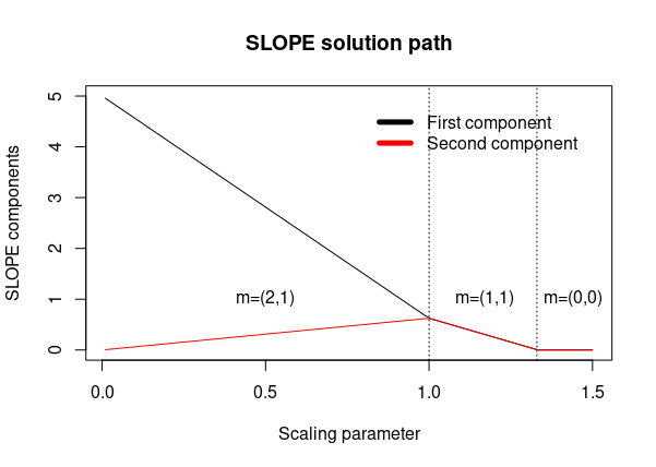
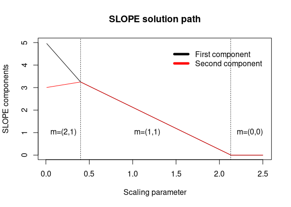
Figure 2: On the left the signal is $\beta=(5,0)^{\prime}$. Based on this figure one may observe that the pattern of $\beta$ cannot be recovered by SLOPE in the noiseless case. Indeed, for $\alpha\in(0,1)$ we have ${\rm patt}(\hat{\beta}(\alpha))=(2,1)^{\prime}$; when $\alpha\in[1,4/3)$ we have ${\rm patt}(\hat{\beta}(\alpha))=(1,1)^{\prime}$ and when $\alpha>4/3$ then $\hat{\beta}(\alpha)=0$. Consequently, for every $\alpha>0$ we have ${\rm patt}(\hat{\beta}(\alpha))\neq{\rm patt}(\beta)=(1,0)^{\prime}$. On the right the signal is $\bar{\beta}=(5,3)^{\prime}$. Based on this figure one may observe that ${\rm patt}(\bar{\beta})$ is recovered by SLOPE in the noiseless case. Indeed, for $\alpha\in(0,0.4)$ we have ${\rm patt}(\hat{\beta}(\alpha))=(2,1)^{\prime}={\rm patt}(\bar{\beta})$.

4 Asymptotic probability on pattern recovery and pattern consistency

In this section we consider two asymptotic scenarios and establish conditions on tuning parameters for which the pattern of $\beta$ is recovered. In Section 4.1 we consider the case where gaps between distinct absolute values of $\beta$ diverge and in Section 4.2 the case where the sample size $n$ diverges. The proofs rely on Theorem 3.1. We show that the positivity and subdifferential conditions are satisfied under our settings. It turns out that for the positivity condition the tuning parameter cannot be too large, while for the subdifferential condition it cannot be too small. In this way we consider a tuning parameter of the form $\alpha\Lambda$, where $\Lambda\in\mathbb{R}^{p+}$ is fixed and $\alpha$ varies. We determine the assumptions for the sequence $(\alpha)$ for which both positivity and subdifferential conditions hold true, i.e. for which the pattern is recovered.

4.1 $X$ is a fixed matrix

The subdifferential condition, given in Theorem 3.1, says that a vector $\pi$ defined in (3.1) belongs to $\partial J_{\alpha\Lambda}(M)$, where $\alpha$ is a scaling parameter. This condition is equivalent to requiring that a vector ${\pi}/\alpha$ is a member of $\partial J_{\Lambda}(M)$. We denote the vector $\pi/\alpha$ by

$$\pi_{\alpha}=X^{\prime}(\tilde{X}_{M}^{\prime})^{+}\tilde{\Lambda}_{M}+\frac{1}{\alpha}X^{\prime}(I_{n}-\tilde{P}_{M})Y=X^{\prime}(\tilde{X}_{M}^{\prime})^{+}\tilde{\Lambda}_{M}+\frac{1}{\alpha}X^{\prime}(I_{n}-\tilde{P}_{M})\varepsilon,$$ (4.1)

where in the latter equality we have used the fact that $(I_{n}-\tilde{P}_{M})$ is a orthogonal projection onto ${\rm col}(\tilde{X}_{M})^{\bot}$ and therefore $(I_{n}-\tilde{P}_{M})X\beta=(I_{n}-\tilde{P}_{M})\tilde{X}_{M}s=0$, where $\beta=U_{M}s$ and $s\in\mathbb{R}^{\|M\|_{\infty}+}$.

By Theorem 3.1, the probability of pattern recovery by SLOPE is upper bounded by

$$\mathbb{P}\left(\exists\hat{\beta}\in S_{X,\alpha\Lambda}(Y)\mbox{ such that }{\rm patt}(\hat{\beta})={\rm patt}(\beta)\right)\leq\begin{cases}\mathbb{P}\left(J_{\Lambda}^{*}(\pi_{\alpha})\leq 1\right),\\ 0\mbox{ if }\tilde{\Lambda}_{M}\notin{\rm col}(\tilde{X}_{M}^{\prime}).\end{cases}$$ (4.2)

The first point in Theorem 4.1 shows that the probability of pattern recovery matches with the upper bound (4.2) when gaps between different absolute values of terms of $\beta$ are large enough. The last point provides pattern consistency by SLOPE.

Theorem 4.1.

Let $X\in\mathbb{R}^{n\times p}$, $0\neq M\in\mathcal{P}_{p}^{\rm SLOPE}$, and $\Lambda=(\lambda_{1},\ldots,\lambda_{p})^{\prime}\in\mathbb{R}^{p+}$. Consider a sequence of signals $(\beta^{(r)})_{r\geq 1}$ with pattern $M$:

$$\beta^{(r)}=U_{M}s^{(r)}\quad\mbox{with}\quad s^{(r)}\in\mathbb{R}^{k+}\mbox{ and }k=\|M\|_{\infty},$$

whose strength is increasing in the following sense:

$$\Delta_{r}=\min_{1\leq i<k}\left(s_{i}^{(r)}-s_{i+1}^{(r)}\right)\overset{r\to\infty}{\longrightarrow}\infty,\mbox{ with the convention }s_{k+1}^{(r)}=0$$

and let $Y^{(r)}=X\beta^{(r)}+\varepsilon$, where $\varepsilon$ is a vector in $\mathbb{R}^{n}$.

1. Sharpness of the upper bound: Let $\alpha>0$. If $\varepsilon$ is random, then the upper bound (4.2) is asymptotically reached:

   $$\lim_{r\to\infty}\mathbb{P}\left(\exists\hat{\beta}\in S_{X,\alpha\Lambda}(Y^{(r)})\mbox{ such that }{\rm patt}(\hat{\beta})=M\right)=\begin{cases}\mathbb{P}\left(J_{\Lambda}^{*}(\pi_{\alpha})\leq 1\right),\\ 0\mbox{ if }\tilde{\Lambda}_{M}\notin{\rm col}(\tilde{X}_{M}^{\prime}).\end{cases}$$

2. Pattern consistency: If $\alpha_{r}\to\infty$, $\alpha_{r}/\Delta_{r}\to 0$ as $r\to\infty$ and

   $$X^{\prime}(\tilde{X}_{M}^{\prime})^{+}\tilde{\Lambda}_{M}\in\mathrm{ri}(\partial{J_{\Lambda}}(M)),$$

   then for any $\varepsilon\in\mathbb{R}^{n}$ we have

   $$\exists\,r_{0}>0\,\,\,\forall\,r\geq r_{0}\,\,\,\exists\,\hat{\beta}\in S_{X,\alpha_{r}\Lambda}(Y^{(r)})\mbox{ such that }{\rm patt}(\hat{\beta})=M.$$

Remark 4.1.

1. The condition $X^{\prime}(\tilde{X}_{M}^{\prime})^{+}\tilde{\Lambda}_{M}\in\mathrm{ri}(\partial{J_{\Lambda}}(M))$, called open irrepresentability condition, is slightly stronger than the irrepresentability condition $X^{\prime}(\tilde{X}_{M}^{\prime})^{+}\tilde{\Lambda}_{M}\in\partial{J_{\Lambda}}(M)$. Note that the tight gap between these conditions is not specific to SLOPE. For instance, for LASSO, the irrepresentability condition which is sufficient for support recovery in the noisy case is stronger than the weak irrepresentability condition for the noiseless case (see [46] pages 190-192 and 244).

2. The open irrepresentability condition $X^{\prime}(\tilde{X}_{M}^{\prime})^{+}\tilde{\Lambda}_{M}\in\mathrm{ri}(\partial{J_{\Lambda}}(M))$ is equivalent to the following computationally verifiable conditions:

   $$\begin{cases}J_{\Lambda}^{*}(X^{\prime}(\tilde{X}_{M}^{\prime})^{+}\tilde{\Lambda}_{M})\leq 1\mbox{ and }\tilde{\Lambda}_{M}\in{\rm col}(\tilde{X}_{M}^{\prime}),\\ \left|\left\{i\in\{1,\ldots,p\}\colon\sum_{j=1}^{i}|X^{\prime}(\tilde{X}_{M}^{\prime})^{+}\tilde{\Lambda}_{M}|_{(j)}=\sum_{j=1}^{i}\lambda_{j}\right\}\right|=\|M\|_{\infty}.\end{cases}$$

   This equivalence follows from Proposition A.2.

3. Let us assume that the distributions of $\varepsilon$ and $-\varepsilon$ are equal. Because the unit ball of the dual sorted $\ell_{1}$ norm is convex, when $J_{\Lambda}^{*}(X^{\prime}(\tilde{X}_{M}^{\prime})^{+}\tilde{\Lambda}_{M})>1$ then, independently on $\alpha>0$, the probability of pattern recovery is smaller than $1/2$, namely

   $$\mathbb{P}\left(\exists\hat{\beta}\in S_{X,\alpha\Lambda}(Y)\mbox{ such that }{\rm patt}(\hat{\beta})=M\right)\leq 1/2.$$

   This inequality corroborates Theorem 2 in [47]. For LASSO, a similar inequality on the probability of sign recovery is given in [38].

4. In Section 5, we illustrate that, under the open irrepresentability condition, one may select $\alpha>0$ to fix the asymptotic probability of pattern recovery at a level arbitrary close to $1$ (a similar result for LASSO is given in [48]).

4.2 ${X}$ is random, $p$ is fixed, $n$ tends to infinity

In this section we discuss asymptotic properties of the SLOPE estimator in the low-dimensional regression model in which $p$ is fixed and the sample size $n$ tends to infinity.

For each $n\geq p$ we consider a linear regression problem

$${Y}_{n}={X}_{n}\beta+\varepsilon_{n},$$ (4.3)

where ${X}_{n}\in\mathbb{R}^{n\times p}$ is a random design matrix. We now list our assumptions:

1. $\varepsilon_{n}=(\epsilon_{1},\ldots,\epsilon_{n})^{\prime}$, where $(\epsilon_{i})_{i}$ are i.i.d. centered with finite variance.

2. A sequence of design matrices ${X}_{1},{X}_{2},\ldots$ satisfies the condition

   $$\frac{1}{n}{X}_{n}^{\prime}{X}_{n}\stackrel{{\scriptstyle\mathbb{P}}}{{\longrightarrow}}{C},$$ (4.4)

   where ${C}$ is a deterministic positive definite symmetric $p\times p$ matrix.

3. For each $j=1,\ldots,p$,

   $$\frac{\max_{i=1,\ldots,n}|X_{ij}^{(n)}|}{\sqrt{\sum_{i=1}^{n}(X_{ij}^{(n)})^{2}}}\stackrel{{\scriptstyle\mathbb{P}}}{{\longrightarrow}}0.$$

4. $({X}_{n})_{n}$ and $(\epsilon_{n})_{n}$ are independent.

We will consider a sequence of tuning parameters $(\Lambda_{n})_{n}$ defined by

$${\Lambda}_{n}=\alpha_{n}{\Lambda},$$

where ${\Lambda}\in\mathbb{R}^{p+}$ is fixed and $(\alpha_{n})_{n}$ is a sequence of positive numbers.

Let $\hat{\beta}^{\rm SLOPE}_{n}$ be an element from the set $S_{{X}_{n},{{\Lambda}_{n}}}({Y}_{n})$ of SLOPE minimizers. Under assumption B1, for large $n$ with high probability, the set $S_{{X}_{n},{{\Lambda}_{n}}}({Y}_{n})$ consists of one element. Indeed, we have

$$\mathbb{P}\left(\ker(X_{n})=\{0\}\right)=\mathbb{P}\left(X_{n}^{\prime}X_{n}\mbox{ is positive definite}\right)\stackrel{{\scriptstyle n\to\infty}}{{\longrightarrow}}1$$

and $\ker({X}_{n})=\{0\}$ ensures existence of the unique SLOPE minimizer. In a natural setting, the strong consistency of $\hat{\beta}^{\rm SLOPE}_{n}$ can be characterized in terms of behaviour of the tuning parameter, see Theorem C.2 or [33, Th. 4.1]. At this point we note that if (4.4) holds almost surely, then condition $\alpha_{n}/n\to 0$ ensures that $\hat{\beta}^{\rm SLOPE}_{n}\stackrel{{\scriptstyle a.s.}}{{\longrightarrow}}\beta$. Thus, if $\beta$ does not have any clusters nor zeros, i.e. $\|{\rm patt}(\beta)\|_{\infty}=p$, then the $\alpha_{n}/n\to 0$ suffices for ${\rm patt}(\hat{\beta}^{\rm SLOPE}_{n})\stackrel{{\scriptstyle a.s.}}{{\longrightarrow}}{\rm patt}(\beta)$. However, if $\|{\rm patt}(\beta)\|<p$, then the situation is more complex as we shall show below.

The first of our asymptotic results concerns the consistency of the pattern recovery by the SLOPE estimator. We note that condition B2 is not necessary for the SLOPE pattern recovery. This assumption was introduced to ensure the existence of a Gaussian vector in the Theorem 4.2 (i).

Theorem 4.2.

Under the assumptions A, B1, C, the following statements hold true.

1. If $B2$ is additionally satisfied and moreover $\alpha_{n}=\sqrt{n}$, then

   $$\lim_{n\to\infty}\mathbb{P}\left({\rm patt}(\hat{\beta}^{\rm SLOPE}_{n})={\rm patt}(\beta)\right)=\mathbb{P}\left(J_{\Lambda}^{*}({Z})\leq 1\right),$$

   where ${Z}\sim\mathrm{N}(CU_{M}(U^{\prime}_{M}CU_{M})^{-1}\tilde{\Lambda}_{M},\sigma^{2}[C-CU_{M}(U^{\prime}_{M}CU_{M})^{-1}U^{\prime}_{M}C])$.

2. Assume

   $${C}{U}_{M}({U}_{M}^{\prime}{C}{U}_{M})^{-1}\tilde{{\Lambda}}_{M}\in\mathrm{ri}(\partial J_{\Lambda}(M)).$$ (4.5)

   The pattern of SLOPE estimator is consistent, i.e.

   $${\rm patt}(\hat{\beta}^{\rm SLOPE}_{n})\stackrel{{\scriptstyle\mathbb{P}}}{{\longrightarrow}}{\rm patt}(\beta),$$

   if and only if

   $$\lim_{n\to\infty}\frac{\alpha_{n}}{n}=0\qquad\mbox{and}\qquad\lim_{n\to\infty}\frac{\alpha_{n}}{\sqrt{n}}=\infty.$$

3. The condition

   $$J_{\Lambda}^{*}\left({C}{U}_{M}({U}_{M}^{\prime}{C}{U}_{M})^{-1}\tilde{{\Lambda}}_{M}\right)\leq 1$$ (4.6)

   is necessary for pattern consistency of SLOPE estimator.

The random vector $Z$ belongs to smallest affine space containing $\partial{J_{\Lambda}}(b)$, i.e. ${\rm aff}(\partial{J_{\Lambda}}(b))=\{v\in\mathbb{R}^{p}\colon U_{M}^{\prime}v=\tilde{\Lambda}_{M}\}$, see Lemma A.3.

Condition (4.5) is the open SLOPE irrepresentability condition in the $n\to\infty$ regime. The above result should be compared with [39, Theorem 1], where the same conditions on the LASSO tuning parameter ensure consistency of sign recovery by LASSO estimator. Below we make a step further and consider the strong consistency of SLOPE pattern recovery by $\hat{\beta}^{\rm SLOPE}_{n}$. Although this was not Zhao’s and Yu’s main focus, it can be deduced from [39, Theorem 1] that if for $c\in(0,1)$ the LASSO tuning parameter $\lambda_{n}$ satisfies $\lambda_{n}/n\to 0$ and $\lambda_{n}/n^{\frac{1+c}{2}}\to\infty$, then under the strong LASSO irrepresentability condition, one has ${\rm sign}(\hat{\beta}^{\rm LASSO}_{n})\stackrel{{\scriptstyle a.s.}}{{\longrightarrow}}{\rm sign}(\beta)$. Even though the patterns are discrete objects, as the underlying probability space is uncountable, the convergence in probability does not imply the almost sure convergence. We show below that if $\alpha_{n}/n\to 0$ and $\alpha_{n}/\sqrt{n}\to\infty$, then ${\rm patt}(\hat{\beta}^{\rm SLOPE}_{n})$ is not strongly consistent and one actually have to impose a slightly stronger condition (4.7).

For the purpose of the a.s. convergence, we strengthen the assumption on design matrices:

1. Assume that the rows of ${X}_{n}$ are independent and that each row of ${X}_{n}$ has the same law as $\xi$, where $\xi$ is a random vector whose components are linearly independent a.s. and that $\mathbb{E}[\xi_{i}^{2}]<\infty$ for $i=1,\ldots,p$.

Remark 4.2.

Under B’, by the strong law of large numbers, we have $n^{-1}{X}_{n}^{\prime}{X}_{n}\stackrel{{\scriptstyle a.s.}}{{\longrightarrow}}{C}$, where ${C}=(C_{ij})_{ij}$ with $C_{ij}=\mathbb{E}[\xi_{i}\xi_{j}]$. Moreover, ${C}$ is positive definite if and only if the random variables $(\xi_{1},\ldots,\xi_{p})$ are linearly independent a.s. Indeed, for $t\in\mathbb{R}^{p}$ we have $t^{\prime}{C}t=\mathbb{E}[(\sum_{i=1}^{p}t_{i}\xi_{i})^{2}]>0$ if and only if $\sum_{i=1}^{p}t_{i}\xi_{i}\neq 0$ a.s. for all $t\in\mathbb{R}^{p}\setminus\{0\}$.

Since B’ ensures that (4.4) holds a.s., it also implies that for large $n$, almost surely there exists a unique SLOPE minimizer. We denote this element by $\hat{\beta}^{\rm SLOPE}_{n}$.

Theorem 4.3.

Under $A$, $B^{\prime}$ and $C$ assume that a sequence $(\alpha_{n})_{n}$ satisfies

$$\lim_{n\to\infty}\frac{\alpha_{n}}{n}=0\qquad\mbox{and}\qquad\lim_{n\to\infty}\frac{\alpha_{n}}{\sqrt{n\log\log n}}=\infty.$$ (4.7)

If (4.5) holds, then the sequence $(\hat{\beta}^{\rm SLOPE}_{n})_{n}$ recovers almost surely the pattern of $\beta$ asymptotically, i.e.

$${\rm patt}(\hat{\beta}^{\rm SLOPE}_{n})\stackrel{{\scriptstyle a.s.}}{{\longrightarrow}}{\rm patt}(\beta).$$ (4.8)

Remark 4.3.

Assume that (4.5) is satisfied and set $\alpha_{n}=c\sqrt{n\log\log n}$ for $c>0$. Then (4.7) is not satisfied and with positive probability, the true SLOPE pattern is not recovered. See also Appendix B, where we present more refined results on the strong consistency of the SLOPE pattern. The $\log\log n$ correction in (4.7) comes from the law of iterated logarithm.

5 Simulation study

This simulation study aims at illustrating Theorems 4.1 and 4.2 and at showing that the results provided in these theorems are somehow unified. Hereafter, we consider the linear regression model $Y=X\beta+\varepsilon$, where $X\in\mathbb{R}^{n\times p}$ and $\varepsilon\in\mathbb{R}^{n}$ has i.i.d. $\mathrm{N}(0,1)$ entries. Up to a constant, we choose components of $\Lambda=(\lambda_{1},\ldots,\lambda_{p})^{\prime}$ as expected values of ordered standard Gaussian statistics. Let $Z_{(1)}\geq\ldots\geq Z_{(p)}$ be ordered statistics of i.i.d. $\mathrm{N}(0,1)$ random variables. An approximation of $\mathbb{E}[Z_{(i)}]$ for some $i\in\{1,\ldots,p\}$, denoted $E(i,p)$, is given hereafter (see [49] and references therein)

$$E(i,p)=-\Phi^{-1}\left(\frac{i-0.375}{p+1-0.750}\right),$$

where $\Phi$ is the cumulative distribution function of a $\mathrm{N}(0,1)$ random variable. We set $\lambda_{i}=E(i,p)+E(p-1,p)-2E(p,p)$ for $i=1,\ldots,p$ (note that $E(1,p)>\ldots>E(p,p)$ thus, $\Lambda=(\lambda_{1},\ldots,\lambda_{p})^{\prime}\in\mathbb{R}^{p+}$).

For the design matrix $X$ and the regression coefficients $\beta$ we consider two cases:

• The design matrix $X$ is orthogonal and components of $\beta$ are all equal with a magnitude tending to infinity.

• The design matrix $X$ is asymptotically orthogonal when the sample size diverges and components of $\beta$ are all equal to $1$.

5.1 Sharp upper bound when $X$ is orthogonal

In Figure 3, $p=100$, $X\in\mathbb{R}^{n\times p}$ is orthogonal (i.e $X^{\prime}X=I_{100}$) and $\beta\in\mathbb{R}^{p}$ is such that $\beta_{1}=\ldots=\beta_{p}=c>0$. To compute the value $\alpha_{0.95}$ of the scaling parameter for which the upper bound is $0.95$ we note that ${\pi}_{\alpha}$ is a Gaussian vector having a $\mathrm{N}\left(X^{\prime}(\tilde{X}_{M}^{\prime})^{+}\tilde{\Lambda}_{M},\alpha^{-2}X^{\prime}(I-\tilde{X}_{M}\tilde{X}_{M}^{+})X\right)$ distribution. Moreover, since $M={\rm patt}(\beta)=(1,\ldots,1)^{\prime}$ we have

$$X^{\prime}(\tilde{X}_{M}^{\prime})^{+}\tilde{\Lambda}_{M} = \left(\frac{1}{p}\sum_{i=1}^{p}\lambda_{i},\ldots,\frac{1}{p}\sum_{i=1}^{p}\lambda_{i}\right)\mbox{ and }$$ (5.1)

$$X^{\prime}(I_{n}-\tilde{X}_{M}\tilde{X}_{M}^{+})X = \begin{pmatrix}1-1/p&-1/p&\ldots&-1/p\\ -1/p&\ddots&\ddots&\vdots\\ \vdots&\ddots&\ddots&-1/p\\ -1/p&\ldots&-1/p&1-1/p\end{pmatrix}.$$

Since the distribution of ${\pi}_{\alpha}$ is given (and the open SLOPE irrepresentability condition occurs), one may pick $\alpha_{0.95}\approx 1.391$ for which $\mathbb{P}(J_{\Lambda}^{*}({\pi}_{\alpha_{0.95}})\leq 1)=0.95$.

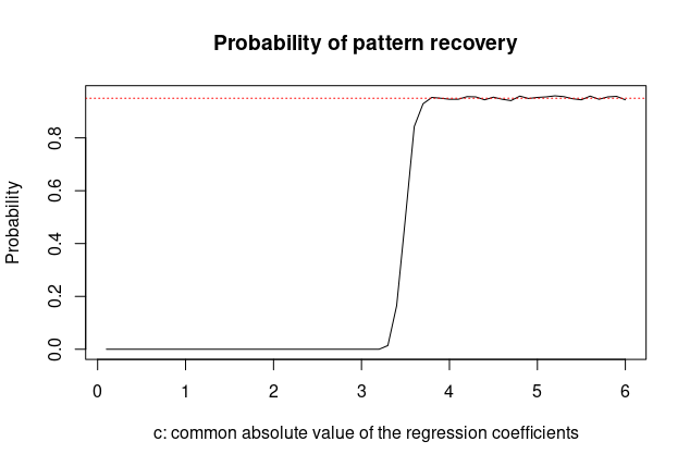
Figure 3: This figure illustrates the estimates of probability of pattern recovery by SLOPE as a function of $c$ where $c=\beta_{1}=\ldots=\beta_{100}>0$ (for each point the probability is computed via $10^{5}$ Monte-Carlo experiments). The scaling parameter $\alpha_{0.95}\approx 1.391$ is chosen to fix the upper bound at a level $0.95$. Note that when $c$ is large, the probability of pattern recovery is approximately equal to $0.95$.

5.2 Limiting probability when $X$ is asymptotically orthogonal

In Figure 4, $X\in\mathbb{R}^{n\times 100}$ has i.i.d. $\mathrm{N}(0,1)$ entries, $\beta_{1}=\ldots=\beta_{100}=1$ and $\alpha_{0.95}\approx 1.391$. Actually, since $n^{-1}X^{\prime}X$ converges to $I_{100}$, when ${\rm patt}(\beta)=(1,\ldots,1)^{\prime}$ the Gaussian vector involved in the limiting probability has the same mean vector and the same covariance matrix as (5.1). Consequently, the scaling parameter $\alpha_{0.95}\approx 1.391$ allows to fix the limiting probability at $0.95$.

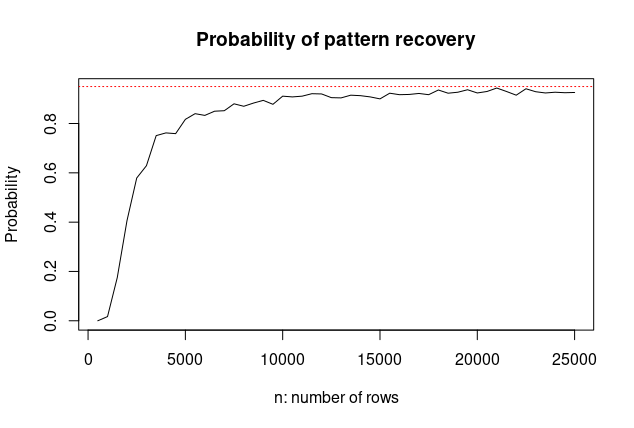
Figure 4: This figure illustrates the estimates of probability of pattern recovery by SLOPE as a function of $n$ (for each point the probability is computed via $10^{3}$ Monte-Carlo experiments). The scaling parameter $\alpha_{0.95}\approx 1.391$ is chosen to fix the limiting probability of pattern recovery at $0.95$. Note that when $n$ is large the probability of pattern recovery is approximately equal to $0.95$.

When $X$ is orthogonal (or asymptotically orthogonal) SLOPE can recover ${\rm patt}(\beta)$ with a probability tending to $1$. Therefore, one may derive from SLOPE a multiple testing procedure to recover the set $\{i\colon|\beta|_{(i)}>|\beta|_{(i+1)}\}$ (similarly as fused LASSO can recover the set $\{i\colon\beta_{i+1}\neq\beta_{i}\}$ [50, 51, 52, 53]). Deriving such a procedure is a perspective for a future work. In Section E, based on above numerical experiments, we provide a testing procedure for

$$\mathcal{H}^{0}:|\{i\colon|\beta|_{(i)}>|\beta|_{(i+1)}\}|=0\quad\mbox{ vs }\quad\mathcal{H}^{1}:|\{i\colon|\beta|_{(i)}>|\beta|_{(i+1)}\}|\geq 1.$$

6 Discussion

In this article we make an important step in understanding the clustering properties of SLOPE and we have shown that the irrepresentability condition provides theoretical guarantees for SLOPE pattern recovery. However, this by no means closes the topic of the SLOPE pattern recovery. Similarly to the irrepresentability condition for LASSO, SLOPE irrepresentability condition is rather stringent and imposes a strict restriction on the number of nonzero clusters in $\beta$. On the other hand, in [48] it is shown that a much weaker condition for LASSO is required to separate the estimators of the null components of $\beta$ from the estimators of nonzero regression coefficients. This condition, called accessibility (also called identifiability), requires that the vector $\beta$ has a minimal $\ell_{1}$ norm among all vectors $\gamma$ such that $X\beta=X\gamma$. Thus, when the accessibility condition is satisfied one can recover the sign of $\beta$ by thresholding LASSO estimates. Empirical results from [48] suggest that this weaker condition is also sufficient for the sign recovery by the adaptive LASSO [40]. In this case rescaling the design matrix according to the initial estimates of regression coefficients modifies the original irrepresentability condition, so it can be satisfied for a given specific true sign vector of regression coefficients. In the recent article [47] it is shown that the similar result holds for SLOPE, whose accessibility condition holds if the vector $\beta$ has the smallest sorted $\ell_{1}$ norm among all vectors $\gamma$ such that $X\beta=X\gamma$. In [47] it is shown that when the accessibility condition is satisfied then SLOPE properly ranks the estimators of regression coefficients and the SLOPE pattern can be recovered by shrinking similar estimates towards the cluster centers.

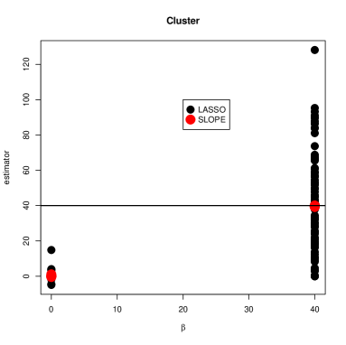
Figure 5: Comparison of LASSO and SLOPE when the cluster structure is present in the data. Here $n=100$, $p=200$, and the correlation between $i^{th}$ and $j^{th}$ column of $X$ is equal to $0.9048^{|i-j|}$. First $k=100$ columns of $X$ are associated with $Y$ and their nonzero regression coefficient are all equal to $40$. The SLOPE and LASSO irrepresentability conditions are not satisfied, but SLOPE, contrary to LASSO, satisfies the admissibility condition.

Figure 5 illustrates this phenomenon and shows that the accessibility condition for SLOPE can be much less restrictive than the accessibility condition for LASSO. In this example the matrix $X$ and the vector $Y$ are generated as in example illustrated in Figure 1 and the only difference is that now first $k=100=n$ regression coefficients are all equal to $40$. In this situation the accessibility condition for LASSO is not satisfied and LASSO can not properly separate the null and nonzero regression coefficients. Also, despite the selection of the tuning parameter so as to minimize the squared estimation error, the precision of LASSO estimates is very poor. As far as SLOPE is concerned, the irrepresentability condition is not satisfied but the accessibility condition holds. Thus, while SLOPE can not properly identify the pattern, it estimates $\beta$ with such a good precision that the difference between the estimated and the true pattern is hardly visible on the graph. These nice ranking and estimation properties of SLOPE bring a promise for efficient pattern recovery by appropriate thresholded SLOPE versions, which are currently under development. We also expect that the mathematical understanding of SLOPE irrepresentability condition presented in this article will lead to the development of efficient adaptive versions of SLOPE, with improved estimation and pattern recovery properties.

The results presented in this article pave the road for a full understanding of the SLOPE pattern recovery properties. We expect that our SLOPE irrepresentability condition will be a basic block for proving further results on the pattern recovery of SLOPE and adaptive SLOPE in the high-dimensional regime. We also look forward the research on other statistical models and loss functions. One specific focus of interest is the graphical SLOPE (see [54]), which could be used for identification of colored graphical models [55], with specific parameter sharing patterns in the precision matrix. Such repetitive patterns occur naturally in many situations, like e.g. in case of the autoregressive type of dependence between variables in the data base or when variables are influenced by the same structural factors. We believe that an efficient exploitation of these unknown patterns by SLOPE will lead to a great reduction of the number of parameters and improvement of the graphical models estimation properties.

Finally, we would like to recall that an interest in identifying the parameter sharing patterns goes beyond classical parametric models and is prevalent also in the modern machine learning community. As mentioned in the introduction, the prominent example is provided by the Convolutional Neural Networks (CNN), where the ”parameter sharing” has allowed to dramatically improve computational and statistical efficiency. While the parameter sharing in CNN is driven entirely by the expert knowledge, regularization by SLOPE allows to identify and exploit patterns based on the data. In principle one can also use SLOPE in the Bayesian context and combine the information in the data with the imprecise prior knowledge on possible parameter sharing patterns (see [56] for the preliminary version of adaptive Bayesian SLOPE). It is expected that recent developments in efficient implementations of the SLOPE optimization algorithm (see, e.g. [57, 58]) will soon allow for an integration of SLOPE regularization with the deep neural networks architecture.

Appendix A Proofs

A.1 Proof of Proposition 2.1

Note that if $M=0$, then the statement holds by (2.1). Thus we may later assume that $M\neq 0$. To ease the notation, we write $\tilde{\Lambda}$ instead of $\tilde{\Lambda}_{M}$. The elements of $\tilde{\Lambda}$ are denoted by $\tilde{\Lambda}_{l}$, $l=1,\ldots,k$. Let $k=\|M\|_{\infty}$. Before proving Proposition 2.1 note that, by assumption, there exists $s\in\mathbb{R}^{k+}$ such that $b=U_{M}s$. Consequently, $|b|_{\downarrow}=U_{|M|_{\downarrow}}s$ and thus

$$J_{\Lambda}(b)=\lambda_{1}|b|_{(1)}+\ldots+\lambda_{p}|b|_{(p)}=\Lambda^{\prime}U_{|M|_{\downarrow}}s=\tilde{\Lambda}^{\prime}s=s_{1}\tilde{\Lambda}_{1}+\ldots+s_{k}\tilde{\Lambda}_{k}.$$

Moreover, with $p_{l}=|\{i\colon|M_{i}|\geq k+1-l\}|$, we have $\tilde{\Lambda}_{l}=\lambda_{p_{l-1}+1}+\ldots+\lambda_{p_{l}}$, $l=1,\ldots,k$.

Proof of Proposition 2.1.

First we prove the inclusion $\partial{J_{\Lambda}}(b)\subset\left\{v\in\mathbb{R}^{p}\colon J_{\Lambda}^{*}(v)\leq 1\mbox{ and }U_{M}^{\prime}v=\tilde{\Lambda}\right\}$. Let $v\in\partial{J_{\Lambda}}(b)$. Since $J^{*}_{\Lambda}(v)\leq 1$ (see (2.1)) then, by definition of the dual sorted $\ell_{1}$ norm, for all $j\in\{1,2,\ldots,p\}$ we have $\sum_{i=1}^{j}|v|_{(i)}\leq\sum_{i=1}^{j}\lambda_{i}$. It remains to prove that $U_{M}^{\prime}v=\tilde{\Lambda}$. For all $l\in\{1,\ldots,k\}$ we have the following inequality

$$\sum\limits_{i=1}^{l}[U^{\prime}_{M}v]_{i}=\sum\limits_{i\colon|M_{i}|\geq k+1-l}{\rm sign}(M_{i})v_{i}\leq\sum\limits_{i\colon|M_{i}|\geq k+1-l}|v_{i}|\\ \leq\sum\limits_{i=1}^{p_{l}}|v|_{(i)}\leq\sum\limits_{i=1}^{p_{l}}\lambda_{i}=\sum\limits_{i=1}^{l}\tilde{\Lambda}_{i}.$$ (A.1)

Note that

$$b^{\prime}v=(U_{M}s)^{\prime}v=\sum_{i=1}^{k}s_{i}[U^{\prime}_{M}v]_{i}=\sum_{l=1}^{k-1}(s_{l}-s_{l+1})\sum_{i=1}^{l}[U^{\prime}_{M}v]_{i}+s_{k}\sum_{i=1}^{k}[U^{\prime}_{M}v]_{i}\\ \leq\sum_{l=1}^{k-1}(s_{l}-s_{l+1})\sum_{i=1}^{l}\tilde{\Lambda}_{i}+s_{k}\sum_{i=1}^{k}\tilde{\Lambda}_{i}=\sum_{l=1}^{k}s_{l}\tilde{\Lambda}_{l}=J_{\Lambda}(b).$$

Moreover, since $v\in\partial{J_{\Lambda}}(b)$, we have $b^{\prime}v=J_{\Lambda}(b)$ (see (2.1)). Therefore

$$\sum_{i=1}^{l}[U^{\prime}_{M}v]_{i}=\sum_{i=1}^{l}\tilde{\Lambda}_{i}\quad\mbox{ for }\quad l=1,\ldots,k$$

and thus the inequalities given in (A.1) are the equalities. Thus

$$[U^{\prime}_{M}v]_{l}=\tilde{\Lambda}_{l}\quad\mbox{ for }\quad l=1,\ldots,k$$

and hence that $U^{\prime}_{M}v=\tilde{\Lambda}$.

Now we prove the other inclusion, $\partial{J_{\Lambda}}(b)\supset\left\{v\in\mathbb{R}^{p}\colon J_{\Lambda}^{*}(v)\leq 1\mbox{ and }U_{M}^{\prime}v=\tilde{\Lambda}_{M}\right\}$. Assume that $v\in\mathbb{R}^{p}$ satisfies $J_{\Lambda}^{*}(v)\leq 1$ and $U^{\prime}_{M}v=\tilde{\Lambda}$. To prove that $v\in\partial{J_{\Lambda}}(b)$ it remains to establish that $b^{\prime}v=J_{\Lambda}(b)$ (see (2.1)). Since $b=U_{M}s$, we have

$$b^{\prime}v=(U_{M}s)^{\prime}v=s^{\prime}U^{\prime}_{M}v=s^{\prime}\tilde{\Lambda}=J_{\Lambda}(b).$$

∎

A.2 Proof of Proposition 2.2

Lemma A.1.

Let $\Lambda\in\mathbb{R}^{p+}$ and $b\in\mathbb{R}^{p}$. If $\Lambda\in\partial{J_{\Lambda}}(b)$ then $b_{1}\geq\ldots\geq b_{p}\geq 0$.

Proof.

Let us assume that $b_{i}<0$ for some $i\in\{1,\ldots,p\}$. For

$$\check{\pi}=(\lambda_{1},\ldots,\lambda_{i-1},-\lambda_{i},\lambda_{i+1},\ldots,\lambda_{p})$$

we have $J_{\Lambda}^{*}(\check{\pi})\leq 1$ and one may deduce that

$$\Lambda^{\prime}b<\check{\pi}^{\prime}b\leq\max\{\pi^{\prime}b\colon J_{\Lambda}^{*}(\pi)\leq 1\}=J_{\Lambda}(b).$$

Consequently $\Lambda\notin\partial{J_{\Lambda}}(b)$ leading to a contradiction. Let us assume that $b_{i}<b_{j}$ for some $1\leq i<j\leq p$. Let us define $\check{\pi}$, where $J_{\Lambda}^{*}(\check{\pi})\leq 1$, as follows

$$\check{\pi}_{k}=\begin{cases}\lambda_{k}&\mbox{ if }k\neq i,k\neq j,\\ \lambda_{j}&\mbox{ if }k=i,\\ \lambda_{i}&\mbox{ if }k=j,\end{cases}\qquad k=1,\ldots,p.$$

Since $\lambda_{i}>\lambda_{j}$, by the rearrangement inequality we have $\lambda_{i}b_{i}+\lambda_{j}b_{j}<\lambda_{j}b_{i}+\lambda_{i}b_{j}$. Thus, one may deduce the following inequality

$$\Lambda^{\prime}b<\check{\pi}^{\prime}b\leq\max\{\pi^{\prime}b\colon\pi\in\mathbb{R}^{p}\,\,J_{\Lambda}^{*}(\pi)\leq 1\}=J_{\Lambda}(b).$$

Consequently $\Lambda\notin\partial{J_{\Lambda}}(b)$ leading to a contradiction. ∎

Let $\psi$ be an orthogonal transformation defined by $\psi\colon\mathbb{R}^{p}\ni b\mapsto(v_{1}b_{r(1)},\ldots,v_{p}b_{r(p)})$ where $v_{1},\ldots,v_{p}\in\{-1,1\}$ and $r$ is a permutation on $\{1,\ldots,p\}$. Before proving Proposition 2.2 let us recall that for any $a,b\in\mathbb{R}^{p}$ we have $J_{\Lambda}(b)=J_{\Lambda}(\psi(b))$, $J_{\Lambda}^{*}(b)=J_{\Lambda}^{*}(\psi(b))$ and $b^{\prime}a=\psi(b)^{\prime}\psi(a)$ implying thus $\partial{J_{\Lambda}}(\psi(b))=\psi(\partial{J_{\Lambda}}(b))$.

Proof of Proposition 2.2.

If ${\rm patt}(a)={\rm patt}(b)$ then, according to Proposition 2.1, $\partial{J_{\Lambda}}(a)=\partial{J_{\Lambda}}(b)$. Let us set $M={\rm patt}(a)$ and $\tilde{M}={\rm patt}(b)$, it remains to prove that if $\partial{J_{\Lambda}}(a)=\partial{J_{\Lambda}}(b)$ then $M=\tilde{M}$. Since the subdifferential $\partial{J_{\Lambda}}(a)$ depends on $a$ only through its pattern, then by Proposition 2.1 we have $\partial{J_{\Lambda}}(a)=\partial{J_{\Lambda}}(M)$ and similarly $\partial{J_{\Lambda}}(b)=\partial{J_{\Lambda}}(\tilde{M})$.

First let us assume that $M=|M|_{\downarrow}$ namely $M_{1}\geq M_{2}\geq\ldots\geq M_{p}\geq 0$. In this case, $M^{\prime}{\Lambda}=J_{{\Lambda}}(M)$ and hence ${\Lambda}=(\lambda_{1},\ldots,\lambda_{p})^{\prime}\in\partial{J_{\Lambda}}(M)$. Since $\partial{J_{\Lambda}}(M)=\partial{J_{\Lambda}}(\tilde{M})$, it follows from Lemma A.1 that $\tilde{M}_{1}\geq\ldots\geq\tilde{M}_{p}\geq 0$, because ${\Lambda}\in\partial{J_{\Lambda}}(\tilde{M})$. To prove that $M=\tilde{M}$, first let us establish that $M_{p}=\tilde{M}_{p}=0$ or $M_{p}=\tilde{M}_{p}=1$. If $M_{p}=0$ and $\tilde{M}_{p}=1$ then, let us set $\check{\pi}=(\lambda_{1},\ldots,\lambda_{p-1},0)^{\prime}$, where $J_{\Lambda}^{*}(\check{\pi})\leq 1$. Because

$$J_{\Lambda}(M)=\Lambda^{\prime}M=\check{\pi}^{\prime}M\mbox{ and }J_{\Lambda}(\tilde{M})=\Lambda^{\prime}\tilde{M}>\check{\pi}^{\prime}\tilde{M}$$

we have $\check{\pi}\in\partial{J_{\Lambda}}(M)$ and $\check{\pi}\notin\partial{J_{\Lambda}}(\tilde{M})$ which provides a contradiction. We proceed analogously for $M_{p}=1$ and $\tilde{M}_{p}=0$. To achieve proving that $M=\tilde{M}$, let us establish that $M_{i}=M_{i+1}$ and $\tilde{M}_{i}=\tilde{M}_{i+1}$ or $M_{i}>M_{i+1}$ and $\tilde{M}_{i}>\tilde{M}_{i+1}$. If $M_{i}=M_{i+1}$ and $\tilde{M}_{i}>\tilde{M}_{i+1}$ then, let us define $\check{\pi}$, where $J_{\Lambda}^{*}(\check{\pi})\leq 1$, as follows

$$\check{\pi}_{k}=\begin{cases}\lambda_{k}&\mbox{ if }k\neq i,k\neq i+1,\\ \lambda_{i+1}&\mbox{ if }k=i,\\ \lambda_{i}&\mbox{ if }k=i+1,\end{cases}\qquad k=1,\ldots,p.$$

Since $\lambda_{i}M_{i}+\lambda_{i+1}M_{i+1}=\lambda_{i+1}M_{i}+\lambda_{i}M_{i+1}$ and $\lambda_{i}\tilde{M}_{i}+\lambda_{i+1}\tilde{M}_{i+1}>\lambda_{i+1}\tilde{M}_{i}+\lambda_{i}\tilde{M}_{i+1}$ then

$$J_{\Lambda}(M)=\Lambda^{\prime}M=\check{\pi}^{\prime}M\mbox{ and }J_{\Lambda}(\tilde{M})=\Lambda^{\prime}\tilde{M}>\check{\pi}^{\prime}\tilde{M}.$$

Consequently $\check{\pi}\in\partial{J_{\Lambda}}(M)$ and $\check{\pi}\notin\partial{J_{\Lambda}}(\tilde{M})$ which provides a contradiction. We proceed analogously for $M_{i}>M_{i+1}$ and $\tilde{M}_{i}=\tilde{M}_{i+1}$. Finally, if $M\neq|M|_{\downarrow}$ then let us pick an orthogonal transformation $\psi$ as defined above for which $\psi(M)=|M|_{\downarrow}$. Since $\partial{J_{\Lambda}}(M)=\partial{J_{\Lambda}}(\tilde{M})$ implies that $\partial{J_{\Lambda}}(\psi(M))=\partial{J_{\Lambda}}(\psi(\tilde{M}))$, the first part of the proof establishes that $\psi(\tilde{M})=\psi(M)$ and thus $M=\tilde{M}$.

∎

Recall that $J_{\Lambda}^{\ast}(x)\leq 1$ if and only if

$$|x|_{(1)}+\ldots{\color[rgb]{0,0,1}+}|x|_{(j)}\leq\lambda_{1}+\ldots+\lambda_{j},\qquad\qquad j=1,\ldots,p.$$ (A.2)

The following result follows from the proof of Proposition 2.1.

Proposition A.2.

Assume $x\in\mathbb{R}^{p}$ satisfies $J_{\Lambda}^{\ast}(x)\leq 1$ and let $b\in\mathbb{R}^{p}$. Then, $x$ belongs to $\partial J_{\Lambda}(b)$ if and only if the following three conditions hold true:

1. If $b_{i}\neq 0$, then ${\rm sign}(x_{i})={\rm sign}(b_{i})$,

2. If $|b_{i}|>|b_{j}|$ then $|x_{i}|\geq|x_{j}|$,

3. The equalities hold in (A.2) for $j\in\{n_{1},n_{2},\ldots,n_{k}\}$, where $n_{j}=|\{i\colon|M_{i}|\geq k+1-j\}|$ with $(M_{1},\ldots,M_{p})^{\prime}={\rm patt}(b)$.

A.3 Proof of Theorem 3.1

Proof of Theorem 3.1.

Necessity. Let us assume that there exists $\hat{\beta}\in S_{X,\Lambda}(Y)$ with ${\rm patt}(\hat{\beta})=M$. Consequently, $\hat{\beta}={U}_{M}s$ for some $s\in\mathbb{R}^{k+}$.

By Proposition 2.2, ${X}^{\prime}({Y}-{X}\hat{\beta})\in\partial{J_{\Lambda}}(\hat{\beta})=\partial{J_{\Lambda}}(M)$. Multiplying this inclusion by ${U}_{M}^{\prime}$, due to (2.2), we get $\tilde{X}_{M}^{\prime}({Y}-{X}\hat{\beta})=\tilde{\Lambda}_{M}$ and so

$$\tilde{X}_{M}^{\prime}{Y}-\tilde{\Lambda}_{M}=\tilde{X}_{M}^{\prime}{X}\hat{\beta}=\tilde{X}_{M}^{\prime}\tilde{X}_{M}s.$$ (A.3)

The positivity condition is proven.

We apply $(\tilde{X}_{M}^{\prime})^{+}$ from the left to (A.3) and use the fact that $\tilde{{P}}_{M}=(\tilde{X}_{M}^{\prime})^{+}\tilde{X}_{M}^{\prime}$ is the projection onto ${\rm col}(\tilde{X}_{M})$. Since ${X}\hat{\beta}\in{\rm col}(\tilde{X}_{M})$, we have $\tilde{{P}}_{M}{X}\hat{\beta}={X}\hat{\beta}$. Thus,

$$\tilde{{P}}_{M}{Y}-(\tilde{X}_{M}^{\prime})^{+}\tilde{\Lambda}_{M}={X}\hat{\beta}.$$

The above equality gives the subdifferential condition:

$$\partial{J_{\Lambda}}(M)\ni{X}^{\prime}({Y}-{X}\hat{\beta}) = {X}^{\prime}({Y}-(\tilde{{P}}_{M}{Y}-(\tilde{X}_{M}^{\prime})^{+}\tilde{\Lambda}_{M}))$$

$$= {X}^{\prime}(\tilde{X}_{M}^{\prime})^{+}\tilde{\Lambda}_{M}+{X}^{\prime}({I}_{n}-\tilde{{P}}_{M})Y=\pi.$$

Sufficiency. Assume that the positivity condition and the subdifferential conditions hold true. Then, by the positivity condition, one may pick $s\in\mathbb{R}^{k+}$ for which

$$\tilde{\Lambda}_{M}=\tilde{X}_{M}^{\prime}{Y}-\tilde{X}_{M}^{\prime}\tilde{X}_{M}s.$$ (A.5)

Let us show that ${U}_{M}s\in S_{X,\Lambda}(Y)$. By definition of ${U}_{M}$, we have ${\rm patt}({U}_{M}s)=M$ thus $\partial{J_{\Lambda}}(U_{M}s)=\partial{J_{\Lambda}}(M)$. Moreover, using (A.3) and (A.5) one may deduce

$$\partial{J_{\Lambda}}(U_{M}s)\ni\pi = {X}^{\prime}({Y}-\tilde{{P}}_{M}{Y}+(\tilde{X}_{M}^{\prime})^{+}\tilde{\Lambda}_{M})$$

$$= {X}^{\prime}({Y}-\tilde{{P}}_{M}{Y}+(\tilde{X}_{M}^{\prime})^{+}(\tilde{X}_{M}Y-\tilde{X}_{M}^{\prime}\tilde{X}_{M}s))$$

$$= X^{\prime}(Y-XU_{M}s).$$

Consequently ${U}_{M}s\in S_{X,\Lambda}(Y)$. ∎

A.4 Proof of Corollary 3.2

Proof of Corollary 3.2.

If SLOPE recovers the pattern of $\beta$ in the noiseless case when $\varepsilon=0$ then, by Theorem 3.1, the subdifferential condition reads as: $X^{\prime}(\tilde{X}_{M}^{\prime})^{+}\tilde{\Lambda}_{M}\in\partial{J_{\Lambda}}(M)$.

Conversely, if $X^{\prime}(\tilde{X}_{M}^{\prime})^{+}\tilde{\Lambda}_{M}\in\partial{J_{\Lambda}}(M)$ then, by Theorem 3.1, it remains to show that the positivity condition occurs for $\alpha>0$ small enough. Since $\beta=U_{M}s$ for some $s\in\mathbb{R}^{k+}$, where $k=\|M\|_{\infty}$, we have

$$\tilde{X}_{M}^{\prime}Y-\alpha\tilde{\Lambda}_{M}=\tilde{X}_{M}^{\prime}\tilde{X}_{M}s-\alpha\tilde{\Lambda}_{M}.$$

Therefore for $\alpha>0$ small enough, $\tilde{X}_{M}^{\prime}Y-\alpha\tilde{\Lambda}_{M}\in\tilde{X}_{M}^{\prime}\tilde{X}_{M}\mathbb{R}^{k+}$ and thus, the positivity condition is proven.

∎

A.5 Proof of Theorem 4.1

Lemma A.3.

Let $0\neq b\in\mathbb{R}^{p}$ and $M={\rm patt}(b)$. Then the smallest affine space containing $\partial{J_{\Lambda}}(b)$ is ${\rm aff}(\partial{J_{\Lambda}}(b))=\{v\in\mathbb{R}^{p}\colon U_{M}^{\prime}v=\tilde{\Lambda}_{M}\}$.

Proof.

According to Proposition 2.1 we have

$${\rm aff}(\partial{J_{\Lambda}}(b))\subset\{v\in\mathbb{R}^{p}\colon U_{M}^{\prime}v=\tilde{\Lambda}_{M}\}.$$

Moreover, according to Theorem 4 in [35] we have

$$\dim({\rm aff}(\partial{J_{\Lambda}}(b)))=\|M\|_{\infty}=\dim(\{v\in\mathbb{R}^{p}\colon U_{M}^{\prime}v=\tilde{\Lambda}_{M}\}),$$

which achieves the proof. ∎

Proof of Theorem 4.1.

(i) Sharpness of the upper bound. According to Theorem 3.1, pattern recovery by SLOPE is equivalent to have simultaneously the positivity condition and the subdifferential condition satisfied. The upper bound (4.2) coincides with the probability of the subdifferential condition. Thus to prove that this upper bound is sharp, it remains to show that the probability of the positivity condition tends to $1$ when $r$ tends to $\infty$. Clearly the upper bound is reached when $\tilde{\Lambda}_{M}\notin{\rm col}(\tilde{X}_{M}^{\prime})$ thus we assume hereafter that $\tilde{\Lambda}_{M}\in{\rm col}(\tilde{X}_{M}^{\prime})$. Recall that $\beta^{(r)}=U_{M}s^{(r)}$ for $s^{(r)}\in\mathbb{R}^{k+}$ and thus $\tilde{X}_{M}^{\prime}Y^{(r)}=\tilde{X}_{M}^{\prime}\tilde{X}_{M}s^{(r)}+\tilde{X}^{\prime}_{M}\varepsilon$. As $\tilde{X}^{\prime}_{M}(\tilde{X}^{\prime}_{M})^{+}=\tilde{X}^{\prime}_{M}\tilde{X}_{M}(\tilde{X}^{\prime}_{M}\tilde{X}_{M})^{+}$ is the projection on ${\rm col}(\tilde{X}_{M}^{\prime})$, we obtain

$$\tilde{X}^{\prime}_{M}Y^{(r)}-\alpha_{r}\tilde{\Lambda}_{M} =\tilde{X}^{\prime}_{M}\tilde{X}_{M}s^{(r)}-\alpha_{r}\tilde{\Lambda}_{M}+\tilde{X}^{\prime}_{M}\varepsilon$$

$$=\tilde{X}^{\prime}_{M}\tilde{X}_{M}s^{(r)}-\alpha_{r}\tilde{X}^{\prime}_{M}\tilde{X}_{M}(\tilde{X}^{\prime}_{M}\tilde{X}_{M})^{+}\tilde{\Lambda}_{M}+\tilde{X}^{\prime}_{M}\tilde{X}_{M}(\tilde{X}^{\prime}_{M}\tilde{X}_{M})^{+}\tilde{X}^{\prime}_{M}\varepsilon$$

$$=\tilde{X}^{\prime}_{M}\tilde{X}_{M}\Delta_{r}\left(\frac{1}{\Delta_{r}}s^{(r)}-\frac{\alpha_{r}}{\Delta_{r}}(\tilde{X}^{\prime}_{M}\tilde{X}_{M})^{+}\tilde{\Lambda}_{M}+\frac{1}{\Delta_{r}}(\tilde{X}^{\prime}_{M}\tilde{X}_{M})^{+}\tilde{X}^{\prime}_{M}\varepsilon\right).$$

Note that by the assumption on $\Delta_{r}$:

• the vector $s^{(r)}/\Delta_{r}\in\mathbb{R}^{k+}$ is (component-wise) larger than or equal to $(k,\ldots,1)$;

• $\lim_{r\to\infty}\alpha_{r}/\Delta_{r}=0$ and $\lim_{r\to\infty}1/\Delta_{r}=0$.

Consequently, for $r$ large enough we have

$$\tilde{X}^{\prime}_{M}Y^{(r)}-\alpha_{r}\tilde{\Lambda}_{M}\in\tilde{X}^{\prime}_{M}\tilde{X}_{M}\mathbb{R}^{k+}.$$

Since this fact is true for any realization of $\varepsilon$, one may deduce that

$$\lim_{r\to\infty}\mathbb{P}\left(\tilde{X}^{\prime}_{M}Y^{(r)}-\alpha_{r}\tilde{\Lambda}_{M}\in\tilde{X}^{\prime}_{M}\tilde{X}_{M}\mathbb{R}^{k+}\right)=1.$$

(ii) Pattern consistency. In the proof of the previous part, we see that positivity condition occurs when $r$ is sufficiently large. Thus it remains to prove that subdifferential condition occurs as $r\to\infty$ when $X^{\prime}(\tilde{X}_{M}^{\prime})^{+}\tilde{\Lambda}_{M}\in\mathrm{ri}(\partial{J_{\Lambda}}(M))$. First we observe that

$$X^{\prime}(\tilde{X}_{M}^{\prime})^{+}\tilde{\Lambda}_{M}+\frac{1}{\alpha_{r}}X^{\prime}(I_{n}-\tilde{P}_{M})\varepsilon\overset{r\to\infty}{\longrightarrow}X^{\prime}(\tilde{X}_{M}^{\prime})^{+}\tilde{\Lambda}_{M}.$$ (A.6)

Note by Lemma A.3 that $X^{\prime}(\tilde{X}_{M}^{\prime})^{+}\tilde{\Lambda}_{M}+\alpha_{r}^{-1}X^{\prime}(I_{n}-\tilde{P}_{M})\varepsilon\in\mathrm{aff}(\partial{J_{\Lambda}}(M))$. Indeed, since $\tilde{\Lambda}_{M}\in{\rm col}(\tilde{X}_{M}^{\prime})$ we have

$$\underbrace{U_{M}^{\prime}X^{\prime}(\tilde{X}_{M}^{\prime})^{+}\tilde{\Lambda}_{M}}_{=\tilde{\Lambda}_{M}}+\frac{1}{\alpha_{r}}\underbrace{U_{M}^{\prime}X^{\prime}(I_{n}-\tilde{P}_{M})\varepsilon(\omega)}_{=0}=\tilde{\Lambda}_{M}.$$

The second term above is zero due to the fact that $(I_{n}-\tilde{P}_{M})$ is an orthogonal projection onto ${\rm col}(\tilde{X}_{M})^{\bot}$. When $X^{\prime}(\tilde{X}_{M}^{\prime})^{+}\tilde{\Lambda}_{M}\in\mathrm{ri}(\partial{J_{\Lambda}}(M))$, due to (A.6), one may deduce that for sufficiently large $r$ we have

$$X^{\prime}(\tilde{X}_{M}^{\prime})^{+}\tilde{\Lambda}_{M}+\frac{1}{\alpha_{r}}X^{\prime}(I_{n}-\tilde{P}_{M})\varepsilon\in\partial{J_{\Lambda}}(M).$$

Consequently, when $r$ is sufficiently large, both the positivity and the subdifferential conditions occur which, by Theorem 3.1, concludes the proof. ∎

A.6 Proofs from Section 4.2

In this part we give proofs of Theorem 4.2 and Theorem 4.3. They are preceded by a series of simple lemmas. For reader’s convenience we recall the setting of Section 4.2.

1. $\varepsilon_{n}=(\epsilon_{1},\ldots,\epsilon_{n})^{\prime}$, where $(\epsilon_{i})_{i}$ are i.i.d. centered with finite variance $\sigma^{2}$.

2. $n^{-1}{X}_{n}^{\prime}{X}_{n}\stackrel{{\scriptstyle\mathbb{P}}}{{\longrightarrow}}{C}>0$.

3. $\frac{\max_{i=1,\ldots,n}|X_{ij}^{(n)}|}{\sqrt{\sum_{i=1}^{n}(X_{ij}^{(n)})^{2}}}\stackrel{{\scriptstyle\mathbb{P}}}{{\longrightarrow}}0$, where ${X}_{n}=(X_{ij}^{(n)})_{ij}$, for each $j=1,\ldots,p.$

4. Rows of ${X}_{n}$ are i.i.d. distributed as $\xi$, where $\xi$ is a random vector whose components are linearly independent a.s. and such that $\mathbb{E}[\xi_{i}^{2}]<\infty$ for $i=1,\ldots,p$.

5. $({X}_{n})_{n}$ and $(\epsilon_{n})_{n}$ are independent.

We consider a sequence of tuning parameters $(\Lambda_{n})_{n}$ defined by ${\Lambda}_{n}=\alpha_{n}{\Lambda}$, where ${\Lambda}\in\mathbb{R}^{p+}$ is fixed and $(\alpha_{n})_{n}$ is a sequence of positive numbers.

To ease the notation, we write the clustered matrices and clustered parameters without the subscript indicating the model $M$, i.e. $\tilde{{\Lambda}}={U}^{\prime}_{|M|\downarrow}{\Lambda}$, $\tilde{{\Lambda}}_{n}=\alpha_{n}\tilde{{\Lambda}}$ and $\tilde{{X}}_{n}={X}_{n}{U}_{M}$.

Lemma A.4.

1. Under A, B1, B2 and C,

   $$\frac{1}{\sqrt{n}}{X}_{n}^{\prime}\varepsilon_{n} \stackrel{{\scriptstyle d}}{{\longrightarrow}}Z\sim\mathrm{N}(0,\sigma^{2}C).$$ (A.7)

2. Under A, B1 and C,

   $$\frac{1}{n}{X}_{n}^{\prime}\varepsilon_{n} \stackrel{{\scriptstyle\mathbb{P}}}{{\longrightarrow}}0.$$ (A.8)

3. Under A, B’ and C,

   $$0<\limsup_{n\to\infty}\frac{\|X_{n}^{\prime}\varepsilon_{n}\|_{\infty}}{\sqrt{n\log\log n}}<\infty\qquad\mbox{a.s.}$$ (A.9)

Proof.

Proof of (A.7). It is enough to show that for any Borel subset $A\subset\mathbb{R}^{p}$ one has

$$\mathbb{P}\left(\frac{1}{\sqrt{n}}{X}_{n}^{\prime}\varepsilon_{n}\in A\mid(X_{n})_{n}\right)\stackrel{{\scriptstyle\mathbb{P}}}{{\longrightarrow}}\mathbb{P}\left(Z\in A\right).$$ (A.10)

Since both sides above are bounded, the convergence in probability implies convergence in $L^{1}$ and therefore establishes (A.7). To show (A.10) we will prove that for any subsequence $(n_{k})_{k}$, there exists a sub-subsequence $(n_{k_{l}})_{l}$ for which, as $l\to\infty$,

$$\mathbb{P}\left(\frac{1}{\sqrt{n_{k_{l}}}}{X}_{n_{k_{l}}}^{\prime}\varepsilon_{n_{k_{l}}}\in A\mid(X_{n})_{n}\right)\stackrel{{\scriptstyle a.s.}}{{\longrightarrow}}\mathbb{P}\left(Z\in A\right).$$ (A.11)

Let $\mathbb{P}_{\mathbf{X}}$ denote the regular conditional probability $\mathbb{P}(\cdot\mid(X_{n})_{n})$ on $(\Omega,\mathcal{F})$. By assumptions B1 and B2, from sequences $(n_{k})_{k}$ one can choose a subsequence $(n_{k_{l}})_{l}$ for which

$$\frac{1}{n_{k_{l}}}{X}_{n_{k_{l}}}^{\prime}{X}_{n_{k_{l}}}\stackrel{{\scriptstyle a.s.}}{{\longrightarrow}}{C}>0\quad\mbox{and}\quad\frac{\max_{i=1,\ldots,{n_{k_{l}}}}|X_{ij}^{({n_{k_{l}}})}|}{\sqrt{\sum_{i=1}^{n_{k_{l}}}(X_{ij}^{({n_{k_{l}}})})^{2}}}\stackrel{{\scriptstyle a.s}}{{\longrightarrow}}0,\quad j=1,\ldots,p.$$

We have

$$\mathrm{Var}_{\mathbf{X}}\left(\frac{1}{\sqrt{n_{k_{l}}}}X^{\prime}_{n_{k_{l}}}\varepsilon_{n_{k_{l}}}\right) =\frac{1}{{n_{k_{l}}}}\mathbb{E}\left[X_{n_{k_{l}}}^{\prime}\varepsilon_{n_{k_{l}}}\varepsilon_{n_{k_{l}}}^{\prime}X_{n_{k_{l}}}\mid(X_{n})_{n}\right]$$

$$=\frac{1}{{n_{k_{l}}}}X_{n_{k_{l}}}^{\prime}\mathbb{E}\left[\varepsilon_{n_{k_{l}}}\varepsilon_{n_{k_{l}}}^{\prime}\right]X_{n_{k_{l}}}=\frac{\sigma^{2}}{{n_{k_{l}}}}X_{n_{k_{l}}}^{\prime}X_{n_{k_{l}}}\stackrel{{\scriptstyle a.s.}}{{\longrightarrow}}\sigma^{2}C>0,$$

and one can apply multivariate Lindeberg-Feller CLT on the space $(\Omega,\mathcal{F},\mathbb{P}_{\mathbf{X}})$ to prove (A.11). Alternatively, the same result follows from [59, Corollary 1.1], which concerns more general Central Limit Theorem for linearly negative quadrant dependent variables with weights forming a triangular array (in particular assumption B2 coincides with [59, (1.8)]).

For (ii) we observe that previous derivations imply that $\mathrm{Var}_{\mathbf{X}}(n^{-1}{X}_{n}^{\prime}\varepsilon_{n})\stackrel{{\scriptstyle\mathbb{P}}}{{\longrightarrow}}0$. We deduce that $\mathbb{P}_{\textbf{X}}(n^{-1}\|{X}_{n}^{\prime}\varepsilon_{n}\|>\delta)\stackrel{{\scriptstyle\mathbb{P}}}{{\longrightarrow}}0$ and hence (ii) follows upon averaging over $({X}_{n})_{n}$.

Eq. (A.9) is the law of iterated logarithm for an i.i.d. sequence $(\xi_{i}\epsilon_{i})_{i}$. ∎

Lemma A.5.

Let $M={\rm patt}(\beta)$. Assume $\alpha_{n}/n\to 0$.

1. Under A, B1 and C, the positivity condition is satisfied for large $n$ with high probability.

2. Under A, B’ and C, the positivity condition is almost surely satisfied for large $n$.

Proof.

If $M=0$, then the positivity condition is trivially satisfied. Thus, we consider $M\neq 0$.

(i) Since $\tilde{{X}}_{n}^{\prime}\tilde{{X}}_{n}$ is invertible for large $n$ with high probability, the positivity condition is equivalent to

$$s_{n}:=(\tilde{{X}}_{n}^{\prime}\tilde{{X}}_{n})^{-1}[\tilde{{X}}_{n}^{\prime}{Y}_{n}-\tilde{{\Lambda}}_{n}]\in\mathbb{R}^{k+}.$$

Let $s_{0}\in\mathbb{R}^{k+}$ be defined through $\beta={U}_{M}s_{0}$, where $k=\|M\|_{\infty}$. We will show that if $\alpha_{n}/n\to 0$, then $s_{n}\stackrel{{\scriptstyle\mathbb{P}}}{{\longrightarrow}}s_{0}$. Since $\mathbb{R}^{k+}$ is an open set, this will imply that for large $n$ with high probability, the positivity condition is satisfied.

First we rewrite $s_{n}$ as

$$s_{n}=(\tilde{{X}}_{n}^{\prime}\tilde{{X}}_{n})^{-1}\tilde{{X}}_{n}^{\prime}{Y}_{n}-\alpha_{n}(\tilde{{X}}_{n}^{\prime}\tilde{{X}}_{n})^{-1}\tilde{{\Lambda}}.$$

Since $\beta={U}_{M}s_{0}$, we conclude ${X}_{n}\beta={X}_{n}{U}_{M}s_{0}=\tilde{{X}}_{n}s_{0}$, so the linear regression model takes the form ${Y}_{n}=\tilde{{X}}_{n}s_{0}+\varepsilon_{n}$. Thus, $(\tilde{{X}}_{n}^{\prime}\tilde{{X}}_{n})^{-1}\tilde{{X}}_{n}^{\prime}{Y}_{n}$ is the OLS estimator of $s_{0}$.

By assumption B and Lemma A.4, we deduce that

$$(\tilde{{X}}_{n}^{\prime}\tilde{{X}}_{n})^{-1}\tilde{{X}}_{n}^{\prime}{Y}_{n}=s_{0}+(n^{-1}\tilde{{X}}_{n}^{\prime}\tilde{{X}}_{n})^{-1}U_{M}\frac{1}{n}X_{n}^{\prime}\varepsilon_{n}\stackrel{{\scriptstyle\mathbb{P}}}{{\longrightarrow}}s_{0}+[({U}_{M}^{\prime}{C}{U}_{M})^{-1}U_{M}]0=s_{0}.$$

To complete the proof, we note that

$$\alpha_{n}(\tilde{{X}}_{n}^{\prime}\tilde{{X}}_{n})^{-1}\tilde{{\Lambda}}=\frac{\alpha_{n}}{n}\left[n(\tilde{{X}}_{n}^{\prime}\tilde{{X}}_{n})^{-1}\tilde{{\Lambda}}\right]\stackrel{{\scriptstyle\mathbb{P}}}{{\longrightarrow}}0\,\left[({U}_{M}^{\prime}{C}{U}_{M})^{-1}\tilde{{\Lambda}}\right]=0.$$

(ii) If one assumes B’ instead of B1, then $n^{-1}{X}_{n}^{\prime}{X}_{n}\stackrel{{\scriptstyle a.s.}}{{\longrightarrow}}C$ and by (A.9), $n^{-1}{X}_{n}^{\prime}\varepsilon_{n}\stackrel{{\scriptstyle a.s.}}{{\longrightarrow}}0$. The result follows along the same lines as (i). ∎

For $M\neq 0$ we denote

$$\pi_{n}^{(1)}={X}_{n}^{\prime}(\tilde{{X}}^{\prime}_{n})^{+}\tilde{{\Lambda}}_{n},\qquad\qquad\pi_{n}^{(2)}={X}^{\prime}_{n}({I}_{n}-\tilde{{P}}_{n}){Y}_{n},$$

$$\pi_{n}=\pi_{n}^{(1)}+\pi_{n}^{(2)},$$

which simplifies in the $M=0$ case to $\pi_{n}=\pi_{n}^{(2)}=X_{n}^{\prime}Y_{n}$.

Recall that the subdifferential condition is equivalent to $J^{*}_{{\Lambda}_{n}}(\pi_{n})\leq 1$ and $\tilde{\Lambda}_{n}\in{\rm col}(\tilde{X}^{\prime}_{M})$ and the latter is satisfied in our setting. Since $\alpha J_{\Lambda}=J_{\alpha\Lambda}$, the subdifferential condition is satisfied if and only if

$$1\geq J^{*}_{{\Lambda}}\left(\alpha_{n}^{-1}\pi_{n}\right)=J^{*}_{{\Lambda}}\left(\alpha_{n}^{-1}\pi_{n}^{(1)}+\frac{\sqrt{n}}{\alpha_{n}}n^{-1/2}\pi_{n}^{(2)}\right).$$

In view of results shown below, $\alpha_{n}^{-1}\pi_{n}^{(1)}$ converges almost surely, while $n^{-1/2}\pi_{n}^{(2)}$ converges in distribution to a Gaussian vector. Thus, the pattern recovery properties of SLOPE estimator strongly depend on the behavior of the sequence $(\alpha_{n}/\sqrt{n})_{n}$.

Lemma A.6.

(a)

1. Assume A, B1 and C. If $M\neq 0$, then

   $$\frac{1}{\alpha_{n}}\pi_{n}^{(1)}\stackrel{{\scriptstyle\mathbb{P}}}{{\longrightarrow}}{C}{U}_{M}({U}_{M}^{\prime}{C}{U}_{M})^{-1}\tilde{\Lambda}.$$

2. Assume A, B1, B2 and C. The sequence $\left(n^{-1/2}\pi_{n}^{(2)}\right)_{n}$ converges in distribution to a Gaussian vector $Z$ with

   $${Z}\sim\mathrm{N}\left(0,\sigma^{2}\left[{C}-{C}{U}_{M}({U}_{M}^{\prime}{C}{U}_{M})^{-1}{U}_{M}^{\prime}{C}\right]\right).$$

3. Assume A, B1 and C. If $\lim_{n\to\infty}{\alpha_{n}}/{\sqrt{n}}=\infty$, then $\alpha_{n}^{-1}\pi_{n}^{(2)}\stackrel{{\scriptstyle\mathbb{P}}}{{\longrightarrow}}0$.

(b) Assume A, B’ and C.

1. If $M\neq 0$, then

   $$\frac{1}{\alpha_{n}}\pi_{n}^{(1)}\stackrel{{\scriptstyle a.s.}}{{\longrightarrow}}{C}{U}_{M}({U}_{M}^{\prime}{C}{U}_{M})^{-1}\tilde{\Lambda}.$$

2. If $\lim_{n\to\infty}{\alpha_{n}}/{\sqrt{n\log\log n}}=\infty$, then $\alpha_{n}^{-1}\pi_{n}^{(2)}\stackrel{{\scriptstyle a.s.}}{{\longrightarrow}}0$.

Proof.

1. Assumption B1 implies that

   $${X}_{n}^{\prime}\tilde{{X}}_{n}(\tilde{{X}}^{\prime}_{n}\tilde{{X}}_{n})^{-1}=\frac{1}{n}{X}_{n}^{\prime}{X}_{n}{U}_{M}({U}_{M}^{\prime}n^{-1}{X}^{\prime}_{n}{X}_{n}{U}_{M})^{-1}\stackrel{{\scriptstyle\mathbb{P}}}{{\longrightarrow}}{C}{U}_{M}({U}_{M}^{\prime}{C}{U}_{M})^{-1}.$$

2. When $\beta={U}_{M}s_{0}$, then the linear regression model takes the form ${Y}_{n}=\tilde{{X}}_{n}s_{0}+\varepsilon_{n}$. Since $\tilde{{P}}_{n}$ is the projection matrix onto ${\rm col}(\tilde{{X}}_{n})$, we have $({I}_{n}-\tilde{{P}}_{n})\tilde{{X}}_{n}=0$. Thus,

   $$n^{-1/2}\pi_{n}^{(2)} =n^{-1/2}{X}_{n}^{\prime}({I}_{n}-\tilde{{P}}_{n}){Y}_{n}=n^{-1/2}{X}_{n}^{\prime}({I}_{n}-\tilde{{P}}_{n})\varepsilon_{n}$$

   $$=\left[{I}_{p}-{X}_{n}^{\prime}{X}_{n}{U}_{M}({U}_{M}^{\prime}{X}_{n}^{\prime}{X}_{n}{U}_{M})^{-1}{U}_{M}^{\prime}\right]\left[n^{-1/2}{X}_{n}^{\prime}\varepsilon\right].$$

   By assumption B1 we have,

   $$n^{-1}{X}_{n}^{\prime}{X}_{n}{U}_{M}({U}_{M}^{\prime}n^{-1}{X}_{n}^{\prime}{X}_{n}{U}_{M})^{-1}{U}_{M}^{\prime}\stackrel{{\scriptstyle\mathbb{P}}}{{\longrightarrow}}{C}{U}_{M}({U}_{M}^{\prime}{C}{U}_{M})^{-1}{U}_{M}^{\prime}.$$ (A.12)

   Thus, by Lemma A.4 (i) and Slutsky’s theorem, we obtain (ii). (iii) follows similarly as A.4 (ii): with the aid of (A.12) we show that $\mathrm{Var}_{\textbf{X}}(\alpha_{n}^{-1}\pi_{n}^{(2)})\stackrel{{\scriptstyle\mathbb{P}}}{{\longrightarrow}}0$, which implies that conditionally on $(X_{n})_{n}$ we have $\alpha_{n}^{-1}\pi_{n}^{(2)}\stackrel{{\scriptstyle\mathbb{P}_{\mathbf{X}}}}{{\longrightarrow}}0$.

   Assumption B’ implies that $n^{-1}{X}_{n}^{\prime}{X}_{n}\stackrel{{\scriptstyle a.s.}}{{\longrightarrow}}C$ and thus (i’) is proven in the same way as (i). (ii’) follows from (A.9).

∎

Proof of Theorem 4.2.

(i) is a direct consequence of Lemmas A.5 and A.6. Since positivity condition is satisfied for large $n$ with high probability, for (ii) we have with $M={\rm patt}(\beta)$,

$$\lim_{n\to\infty}\mathbb{P}\left({\rm patt}(\hat{\beta}^{\rm SLOPE}_{n})=M\right) =\lim_{n\to\infty}\mathbb{P}\left(\pi_{n}\in\partial J_{\alpha_{n}\Lambda}(M)\right)=\lim_{n\to\infty}\mathbb{P}\left(\alpha_{n}^{-1}\pi_{n}\in\partial J_{\Lambda}(M)\right)$$ (A.13)

$$\geq\lim_{n\to\infty}\mathbb{P}\left(\alpha_{n}^{-1}\pi_{n}\in\mathrm{ri}(\partial J_{\Lambda}(M))\right)=1,$$

where in the last equality we use the Portmanteau Theorem, assumption (4.5) and the fact that sequence $(\alpha_{n}^{-1}\pi_{n})_{n}$ converges in distribution to ${C}{U}_{M}({U}_{M}^{\prime}{C}{U}_{M})^{-1}$ if and only if $\alpha_{n}/\sqrt{n}\to\infty$.

Condition (4.6) implies that ${C}{U}_{M}({U}_{M}^{\prime}{C}{U}_{M})^{-1}\in\partial J_{\Lambda}(M)$. Since $(\alpha_{n}^{-1}\pi_{n})_{n}$ converges in probability to ${C}{U}_{M}({U}_{M}^{\prime}{C}{U}_{M})^{-1}$, the necessity of this condition is explained by (A.13). ∎

Proof of Theorem 4.3.

By Lemma A.5, the positivity condition is satisfied for large $n$ almost surely. By Lemma A.6 (i) and (iii), we have

$$a_{n}:=\frac{1}{\alpha_{n}}\pi_{n}\stackrel{{\scriptstyle a.s.}}{{\longrightarrow}}{C}{U}_{M}({U}_{M}^{\prime}{C}{U}_{M})^{-1}\tilde{{\Lambda}}=:a_{0}.$$

It is easy to see that $U_{M}^{\prime}a_{n}=\tilde{\Lambda}$. By the condition $a_{0}\in\mathrm{ri}(J_{\Lambda}(M))$ it follows that $a_{n}\in J_{\Lambda}(M)$ almost surely for sufficiently large $n$. Therefore $\pi_{n}\in J_{\Lambda_{n}}(M)$ for large $n$ almost surely and thus the subdifferential condition is also satisfied.

∎

Appendix B Refined results on strong consistency of the SLOPE pattern

In this appendix we aim to give weaker assumptions on the design matrix than condition B’, but which ensure the almost sure convergence of the pattern of $\hat{\beta}^{\rm SLOPE}_{n}$.

1. $\varepsilon_{n}=(\epsilon_{1},\ldots,\epsilon_{n})^{\prime}$, where $(\epsilon_{i})_{i}$ are independent random variables such that

   $$\mathbb{E}[\epsilon_{n}]=0\quad\mbox{and}\quad\mathrm{Var}(\epsilon_{n})=\sigma^{2}\quad\mbox{for all $n$,}\quad\mbox{ and }\sup_{n}\mathbb{E}[|\epsilon_{n}|^{r}]<\infty$$ (B.1)

   for some $r>2$.

2. A sequence of design matrices ${X}_{1},{X}_{2},\ldots$ satisfies the condition

   $$\frac{1}{n}{X}_{n}^{\prime}{X}_{n}\stackrel{{\scriptstyle a.s.}}{{\longrightarrow}}{C},$$ (B.2)

   where ${C}$ is a deterministic positive definite symmetric $p\times p$ matrix.

   With ${X}_{n}=\left(X_{ij}^{(n)}\right)_{ij}$,

   $$\lim_{n\to\infty}\frac{(\log n)^{\rho}}{\sqrt{n}}\sup_{i,j}\left|X_{ij}^{(n)}\right|=0\quad\mbox{a.s. for all $\rho>0$}$$ (B.3)

   and there exist nonnegative random variables $(c_{i})_{i}$, constants $d>2/r$ and $m_{0}\in\mathbb{N}$ such that for $n>m\geq m_{0}$,

   $$\sup_{j}\left[\sum_{i=1}^{m}\left(X_{ij}^{(n)}-X_{ij}^{(m)}\right)^{2}+\sum_{i=m+1}^{n}\left(X_{ij}^{(n)}\right)^{2}\right]\leq\left(\sum_{i=m+1}^{n}c_{i}\right)^{d}\quad\mbox{ a.s.},$$ (B.4)

   $$\left(\sum_{i=m_{0}}^{n}c_{i}\right)^{d}=O(n)\quad\mbox{a.s.}$$ (B.5)

3. $({X}_{n})_{n}$ and $(\epsilon_{n})_{n}$ are independent.

We note that conditions (B.3) and (B.4) are trivially satisfied in the i.i.d. rows setting of Remark 4.2 or assumption B’. The main ingredient of the proof of the strong pattern consistency is the law of iterated logarithm (A.9) which holds trivially under B’. Below, we establish the same result under more general B”. The technical assumption (B.4) is a kind of weak continuity assumption on the rows of ${X}_{n}$ as it says that the $\ell_{2}$-distance between $j$th rows of ${X}_{n}$ and ${X}_{m}$ should not be too large.

Lemma B.1.

Assume A’, B” and C. Then

$$\limsup_{n\to\infty}\frac{\|X_{n}^{\prime}\varepsilon_{n}\|_{\infty}}{\sqrt{n\log\log n}}<\infty\qquad\mbox{a.s.}$$ (B.6)

Proof.

In view of (4.4) we have for $j=1,\ldots,p$,

$$n^{-1}A_{n}^{(j)}:=n^{-1}\sum_{i=1}^{n}\left(X_{ij}^{(n)}\right)^{2}=\left(n^{-1}{X}_{n}^{\prime}{X}_{n}\right)_{jj}\stackrel{{\scriptstyle a.s.}}{{\longrightarrow}}C_{jj}>0.$$ (B.7)

We apply the general law of iterated logarithm for weights forming a triangular array from [60]. The result follows directly from [60, Theorem 1]. Defining $a_{ni}^{(j)}:=X_{ij}^{(n)}$ for $i=1,\ldots,n$, $j=1,\ldots,p$, $n\geq 1$ and $0$ otherwise, we have

$$({X}_{n}^{\prime}\varepsilon_{n})_{j}=\sum_{i=-\infty}^{\infty}a_{ni}^{(j)}\epsilon_{i}$$

and therefore we fall within the framework of [60, Eq. (1.3)]. Then, (B.1), (B.3), (B.4) and (B.5) coincide with [60, (1.2), (1.6), (1.7), (1.8)] respectively. Let $\mathbb{P}(\cdot|({X}_{n})_{n})$ be a regular conditional probability. Then, applying [60, Theorem 1 (i)] on the probability space $(\Omega,\mathcal{F},\mathbb{P}_{\mathbf{X}})$ to our sequence we obtain that for $j=1,\ldots,n$,

$$\mathbb{P}\left(\limsup_{n\to\infty}\frac{\left|({X}_{n}^{\prime}\varepsilon_{n})_{j}\right|}{\sqrt{2A_{n}^{(j)}\log\log A_{n}^{(j)}}}\leq\sigma\Bigg{|}({X}_{n})_{n}\right)=1\qquad\mbox{a.s.}$$

Averaging over $({X}_{n})_{n}$ and using (B.7) again, we obtain the assertion. ∎

Theorem B.2.

Assume A’, B” and C. Suppose that $(\alpha_{n})_{n}$ satisfies

$$\lim_{n\to\infty}\frac{\alpha_{n}}{n}=0\qquad\mbox{and}\qquad\lim_{n\to\infty}\frac{\alpha_{n}}{\sqrt{n\log\log n}}=\infty.$$

If (4.5) is satisfied, then ${\rm patt}(\hat{\beta}^{\rm SLOPE}_{n})\stackrel{{\scriptstyle a.s.}}{{\longrightarrow}}{\rm patt}(\beta)$.

Comments:

1. Under reasonable assumptions (see e.g. [60, Theorem 1 (iii)]) one can show that

   $$\limsup_{n\to\infty}\frac{\|X_{n}^{\prime}\varepsilon_{n}\|_{\infty}}{\sqrt{n\log\log n}}>0\qquad\mbox{a.s.}$$

   Since $\alpha_{n}^{-1}{X}_{n}^{\prime}\varepsilon_{n}\stackrel{{\scriptstyle a.s.}}{{\longrightarrow}}0$ is necessary for the a.s. pattern recovery, we can show that the condition $\alpha_{n}/\sqrt{n\log\log n}\to\infty$ cannot be weakened. Thus, the gap between the convergence in probability and the a.s. convergence is integral to the problem and in general cannot be reduced.

2. One can relax assumption B” by imposing stronger conditions on the error $\varepsilon_{n}$. E.g. if $\varepsilon_{n}$ is Gaussian, then one can use results from [61]. We note that [61] offers a very similar result as [60], but their assumptions are not quite comparable, see [61, Section 3 i)] for detailed discussion.

3. For Gaussian errors, one can consider a more general setting where one does not assume any relation between $\varepsilon_{n}$ and $\varepsilon_{n+1}$, i.e. the error need not be incremental. For orthogonal design such approach was taken in [33]. It is proved there that one obtains the a.s. SLOPE pattern consistency with the second limit condition of Theorem B.2 replaced by $\lim_{n\to\infty}\alpha_{n}/\sqrt{n\log n}=\infty$. This result can be generalized to non-orthogonal designs.

Appendix C Strong consistency of SLOPE estimator

Lemma C.1.

Assume that $\varepsilon_{n}=(\epsilon_{1},\ldots,\epsilon_{n})^{\prime}$ with $(\epsilon)_{i}$ i.i.d., centered and having finite variance. Suppose

$$\frac{1}{n}{X}_{n}^{\prime}{X}_{n}\stackrel{{\scriptstyle a.s.}}{{\longrightarrow}}C>0.$$ (C.1)

and that $(\varepsilon_{n})_{n}$ and $({X}_{n})_{n}$ are independent. Then $n^{-1}{X}_{n}^{\prime}\varepsilon_{n}\stackrel{{\scriptstyle a.s.}}{{\longrightarrow}}0$.

Proof.

Let $\mathbb{P}(\cdot\mid({X}_{n})_{n})$ denote the regular conditional probability. By [62, Th. 1.1] applied to a sequence $(n^{-1}{X}_{n}^{\prime}\varepsilon_{n})_{j}$ on the probability space $(\Omega,\mathcal{F},\mathbb{P}(\cdot\mid({X}_{n})_{n}))$, we obtain

$$\mathbb{P}\left(\lim_{n\to\infty}n^{-1}({X}_{n}^{\prime}\varepsilon_{n})_{j}=0\mid({X}_{n})_{n}\right)=1,\qquad j=1,\ldots,p,\qquad\mbox{a.s.}$$

Thus, applying the expectation to both sides above we obtain the assertion. ∎

Theorem C.2.

Assume that ${Y}_{n}={X}_{n}\beta+\varepsilon_{n}$, where $\beta\in\mathbb{R}^{p}$, $\varepsilon_{n}=(\epsilon_{1},\ldots,\epsilon_{n})^{\prime}$ with $(\epsilon)_{i}$ i.i.d., centered and finite variance. Suppose (C.1) and that $(\varepsilon_{n})_{n}$ and $({X}_{n})_{n}$ are independent. Let ${\Lambda}_{n}=(\lambda_{1}^{(n)},\ldots,\lambda_{p}^{(n)})^{\prime}$. Then, for large $n$, $S_{{X}_{n},{{\Lambda}_{n}}}({Y}_{n})=\{\hat{\beta}^{\rm SLOPE}_{n}\}$ almost surely.

If $\beta\neq 0$, then $\hat{\beta}^{\rm SLOPE}_{n}\stackrel{{\scriptstyle a.s.}}{{\longrightarrow}}\beta$ if and only if

$$\lim_{n\to\infty}\frac{\lambda_{1}^{(n)}}{n}=0.$$ (C.2)

If $\beta=0$ and (C.2) holds true, then $\hat{\beta}^{\rm SLOPE}_{n}\stackrel{{\scriptstyle a.s.}}{{\longrightarrow}}0$.

Proof of Theorem C.2.

The assumption (C.1) implies that the matrix $X_{n}^{\prime}X_{n}$ is positive definite for large $n$ almost surely and hence ensuring that $\ker({X}_{n})=\{0\}$. It is known that under trivial kernel, the set of SLOPE minimizers contains one element only.

By Proposition 2.1, $\hat{\beta}^{\rm SLOPE}_{n}$ is the SLOPE estimator of $\beta$ in a linear regression model ${Y}_{n}={X}_{n}\beta+\varepsilon_{n}$ if and only if for $\pi_{n}={X}_{n}^{\prime}({Y}_{n}-{X}_{n}\hat{\beta}^{\rm SLOPE}_{n})$ we have

$$J_{\Lambda}^{*}(\pi_{n})\leq 1$$ (C.3)

and

$${U}_{M_{n}}^{\prime}\pi_{n}=\tilde{\Lambda}_{n},$$ (C.4)

where $M_{n}={\rm patt}(\hat{\beta}^{\rm SLOPE}_{n})$ and $\tilde{\Lambda}_{n}=U_{|M_{n}|\downarrow}^{\prime}{\Lambda}_{n}$. By the definition of $\pi_{n}$ we have

$$\hat{\beta}^{\rm SLOPE}_{n}=(X_{n}^{\prime}X_{n})^{-1}X_{n}^{\prime}Y_{n}-(X_{n}^{\prime}X_{n})^{-1}\pi_{n}=\hat{\beta}^{\rm OLS}_{n}-\left(\frac{1}{n}X_{n}^{\prime}X_{n}\right)^{-1}\left(\frac{1}{n}\pi_{n}\right).$$

Since in our setting $\hat{\beta}^{\rm OLS}_{n}$ is strongly consistent, $\hat{\beta}^{SLOPE}_{n}\stackrel{{\scriptstyle a.s.}}{{\longrightarrow}}\beta$ if and only if
$(n^{-1}X_{n}^{\prime}X_{n})^{-1}\left(n^{-1}\pi_{n}\right)\stackrel{{\scriptstyle a.s.}}{{\longrightarrow}}0$. In view of (C.1), we have $(n^{-1}X_{n}^{\prime}X_{n})^{-1}\left(n^{-1}\pi_{n}\right)\stackrel{{\scriptstyle a.s.}}{{\longrightarrow}}0$ if and only if $n^{-1}\pi_{n}\stackrel{{\scriptstyle a.s.}}{{\longrightarrow}}0$.

Assume $n^{-1}\lambda_{1}^{(n)}\to 0$. By (C.3) we have $\|\pi^{n}\|_{\infty}\leq\lambda_{1}^{(n)}$, which gives

$$\left\|\frac{\pi_{n}}{n}\right\|_{\infty}\leq\frac{\lambda_{1}^{(n)}}{n}\to 0.$$

Therefore, (C.2) implies that $\hat{\beta}^{SLOPE}_{n}\stackrel{{\scriptstyle a.s.}}{{\longrightarrow}}\beta$.

Now assume that $\beta\neq 0$ and $\hat{\beta}^{\rm SLOPE}$ is strongly consistent, i.e. $n^{-1}\pi_{n}\stackrel{{\scriptstyle a.s.}}{{\longrightarrow}}0$. Then, (C.4) gives

$$p\|\pi_{n}\|_{\infty}\geq\|U_{M_{n}}^{\prime}\pi_{n}\|_{\infty}=\|\tilde{\Lambda}_{n}\|_{\infty}\geq\lambda_{1}^{(n)}$$ (C.5)

provided $M_{n}\neq 0$. Applying (C.3) for $\hat{\beta}^{SLOPE}_{n}=0$, we note that $M_{n}(\omega)=0$ if and only if

$$J_{n^{-1}\Lambda_{n}}^{*}\left(n^{-1}X_{n}(\omega)^{\prime}Y_{n}(\omega)\right)\leq 1.$$

In view of Lemma C.1, it can be easily verified that $n^{-1}X_{n}^{\prime}Y_{n}\stackrel{{\scriptstyle a.s.}}{{\longrightarrow}}C\beta$. Since

$$\left\|\frac{1}{n}\pi_{n}\right\|_{\infty}\quad\geq\quad\left\|\frac{1}{n}\pi_{n}\right\|_{\infty}{\bf 1}_{(M_{n}=0)}\quad=\quad\left\|\frac{1}{n}X_{n}^{\prime}Y_{n}\right\|_{\infty}{\bf 1}_{(M_{n}=0)},$$

we see that for $\beta\neq 0$, we have $M_{n}\neq 0$ for large $n$ almost surely. Thus, for $\beta\neq 0$ we eventually obtain for large $n$

$$\frac{\lambda_{1}^{(n)}}{n}\leq p\left\|\frac{\pi_{n}}{n}\right\|_{\infty}\quad\mbox{a.s.}$$

∎

Appendix D Geometrical interpretation of ${X}^{\prime}(\tilde{X}_{M}^{\prime})^{+}\tilde{\Lambda}_{M}$

Let $0\neq\beta\in\mathbb{R}^{p}$ where ${\rm patt}(\beta)=M$. For a SLOPE minimizer $\hat{\beta}\in S_{{X},\alpha\Lambda}(X\beta)$ the following occurs:

$$\frac{1}{\alpha}X^{\prime}X(\beta-\hat{\beta})\in\partial{J_{\Lambda}}(\hat{\beta}).$$

In addition when ${\rm patt}(\hat{\beta})=M$, then the following facts hold:

• $\beta-\hat{\beta}\in{\rm col}(U_{M})$, so that $\frac{1}{\alpha}X^{\prime}X(\beta-\hat{\beta})\in{X}^{\prime}{X}\,{\rm col}(U_{M})$.

• $\partial{J_{\Lambda}}(\hat{\beta})=\partial{J_{\Lambda}}(M)$.

Therefore, the noiseless pattern recovery by SLOPE clearly implies that the vector space $X^{\prime}X{\rm col}(U_{M})={\rm col}(X^{\prime}\tilde{X}_{M})$ intersects $\partial{J_{\Lambda}}(M)$. Actually, the vector $\bar{\Pi}=X^{\prime}(\tilde{X}^{\prime}_{M})^{+}\tilde{\Lambda}_{M}$ appearing in Corollary 3.2 has a geometrical interpretation given in Proposition D.1.

Proposition D.1.

Let $X\in\mathbb{R}^{n\times p}$, $0\neq M\in\mathcal{P}^{\rm SLOPE}_{p}$ and $\Lambda\in\mathbb{R}^{p+}$. We recall that $\tilde{X}_{M}=XU_{M}$, $\tilde{\Lambda}_{M}=U_{|M|_{\downarrow}}^{\prime}\Lambda$ and $\bar{\Pi}=X^{\prime}(\tilde{X}^{\prime}_{M})^{+}\tilde{\Lambda}_{M}$. We have the following statements:

1. If $\tilde{\Lambda}_{M}\notin{\rm col}(\tilde{X}_{M}^{\prime})$ then ${\rm aff}(\partial{J_{\Lambda}}(M))\cap{\rm col}(X^{\prime}\tilde{X}_{M})=\emptyset$.

2. If $\tilde{\Lambda}_{M}\in{\rm col}(\tilde{X}_{M}^{\prime})$ then ${\rm aff}(\partial{J_{\Lambda}}(M))\cap{\rm col}(X^{\prime}\tilde{X}_{M})=\{\bar{\Pi}\}$.

3. Pattern recovery by SLOPE in the noiseless case is equivalent to ${\rm col}(X^{\prime}\tilde{X}_{M})\cap\partial{J_{\Lambda}}(M)\not=\emptyset$.

Proof.

i) We recall that, according to Lemma A.3, ${\rm aff}(\partial{J_{\Lambda}}(M))=\{v\in\mathbb{R}^{p}\colon U_{M}^{\prime}v=\tilde{\Lambda}_{M}\}$. If ${\rm aff}(\partial{J_{\Lambda}}(M))\cap{\rm col}(X^{\prime}\tilde{X}_{M})\neq\emptyset$ then there exists $z\in\mathbb{R}^{k}$, where $k=\|M\|_{\infty}$, such that $X^{\prime}\tilde{X}_{M}z\in{\rm aff}(\partial{J_{\Lambda}}(M))$. Consequently, $\tilde{\Lambda}_{M}=U_{M}^{\prime}X^{\prime}\tilde{X}_{M}z=\tilde{X}_{M}^{\prime}\tilde{X}_{M}^{\prime}z$ thus $\tilde{\Lambda}_{M}\in{\rm col}(\tilde{X}_{M}^{\prime})$ which establishes i).
ii) If $\tilde{\Lambda}_{M}\in{\rm col}(\tilde{X}_{M}^{\prime})$ then $\bar{\Pi}\in{\rm aff}(\partial{J_{\Lambda}}(M))$. Indeed, since $\tilde{X}_{M}^{\prime}(\tilde{X}_{M}^{\prime})^{+}$ is the projection on ${\rm col}(\tilde{X}_{M}^{\prime})$ we have

$$U_{M}^{\prime}\bar{\Pi}=\tilde{X}_{M}^{\prime}(\tilde{X}_{M}^{\prime})^{+}\tilde{\Lambda}_{M}=\tilde{\Lambda}_{M}.$$

Moreover, since ${\rm col}((\tilde{X}_{M}^{\prime})^{+})={\rm col}(\tilde{X}_{M})$ we deduce that $\bar{\Pi}\in{\rm col}(X^{\prime}\tilde{X}_{M})$. To prove that $\bar{\Pi}$ is the unique point in the intersection, let us prove that ${\rm col}(X^{\prime}\tilde{X}_{M})\cap{\rm col}(U_{M})^{\perp}=\{0\}$. Indeed, if $v\in{\rm col}(X^{\prime}\tilde{X}_{M})\cap{\rm col}(U_{M})^{\perp}$ then $v=X^{\prime}\tilde{X}_{M}z$ for some $z\in\mathbb{R}^{k}$ and $U_{M}^{\prime}v=0$. Therefore, $\tilde{X}_{M}^{\prime}\tilde{X}_{M}z=0$, consequently $\tilde{X}_{M}z=0$ and thus $v=\{0\}$. Finally, if $\Pi\in{\rm aff}(\partial{J_{\Lambda}}(M))\cap{\rm col}(X^{\prime}\tilde{X}_{M})$ then $\Pi-\bar{\Pi}\in{\rm col}(X^{\prime}\tilde{X}_{M})$ and $U_{M}^{\prime}(\Pi-\bar{\Pi})=0$ which implies that $\Pi=\bar{\Pi}$ and establishes ii).

According to Corollary 3.2, pattern recovery by SLOPE in the noiseless case is equivalent to $\bar{\Pi}\in\partial{J_{\Lambda}}(M)$ which is equivalent, by i) and ii), to ${\rm col}(X^{\prime}\tilde{X}_{M})\cap\partial{J_{\Lambda}}(M)\not=\emptyset$. ∎

Example D.1.

• We observe on the right picture in Fig. 2 that the noiseless pattern recovery occurs when $\bar{\beta}=(5,3)^{\prime}$ (thus $M={\rm patt}(\bar{\beta})=(2,1)^{\prime}$). To corroborate this fact note that $\tilde{X}_{M}=X$ thus ${\rm col}(X^{\prime}\tilde{X}_{M})=\mathbb{R}^{2}$ and consequently ${\rm col}(X^{\prime}\tilde{X}_{M})$ intersects $\partial{J_{\Lambda}}(M)$.

• We observe on the left picture in Fig. 2 that the noiseless pattern recovery does not occur when $\beta=(5,0)^{\prime}$ (thus $M={\rm patt}(\beta)=(1,0)^{\prime}$). To corroborate this fact, Figure 6 illustrates that ${\rm col}(X^{\prime}\tilde{X}_{M})={\rm col}((1,0.6)^{\prime})$ does not intersect $\partial{J_{\Lambda}}(M)=\{4\}\times[-2,2]$.

Figure 6: This figure illustrates $\bar{\Pi}$ in purple as the unique intesection point between ${\rm col}(X^{\prime}\tilde{X}_{M})={\rm col}((1,0.6)^{\prime})$ in blue and ${\rm aff}(\partial{J_{\Lambda}}(M))$ in red. Since $\bar{\Pi}\notin\partial{J_{\Lambda}}(M)=\{4\}\times[-2,2]$ then, in the noiseless case, SLOPE cannot recover $M={\rm patt}(\beta)=(1,0)^{\prime}$.

Appendix E Testing procedure when the design is orthogonal

We consider the same simulation setup as in Section 5: $Y=X\beta+\varepsilon$ where $X\in\mathbb{R}^{n\times 100}$ is an orthogonal matrix and $\varepsilon\in\mathbb{R}^{n}$ has i.i.d. $\mathrm{N}(0,1)$ entries.

Based on SLOPE $\hat{\beta}^{\rm SLOPE}$ (which is uniquely defined when $X$ is orthogonal) we would like to test:

$$\mathcal{H}^{0}\colon|\beta_{1}|=\ldots=|\beta_{p}|=\|\beta\|_{\infty}\mbox{ vs }\mathcal{H}^{1}\colon\exists i\in\{1,\ldots,p\},\,|\beta_{i}|<\|\beta\|_{\infty}.$$

Given $\Lambda\in\mathbb{R}^{p+}$, we reject the null hypothesis when $|\hat{\beta}^{\rm SLOPE}(\alpha_{\eta})|_{(1)}>|\hat{\beta}^{\rm SLOPE}(\alpha_{\eta})|_{(p)}$, where $\alpha_{\eta}>0$ is an appropriately chosen scaling parameter allowing to control the type I error at level $\eta\in(0,1)$.

Prescription for $\Lambda\in\mathbb{R}^{p+}$: As in Section 5 we suggest the tuning parameter: $\lambda_{i}=E(i,p)+E(p-1,p)-2E(p,p)$, $i=1,\ldots,p$ where $E(i,p)$ (approximating the expected value of a standard Gaussian ordered statistic) is defined hereafter

$$E(i,p)=-\Phi^{-1}\left(\frac{i-0.375}{p+1-0.750}\right).$$

The Cesàro sequence $(\frac{1}{i}\sum_{j=1}^{i}(|\hat{\beta}^{\rm OLS}|_{(j)}-\alpha\lambda_{j}))_{1\leq i\leq p}$ is closely related to the explicit expression of SLOPE $\hat{\beta}^{\rm SLOPE}(\alpha)$ when $X$ is orthogonal [43, 44]. Intuitively, using the prescribed tuning parameter $\Lambda$ and under the null hypothesis, when $\alpha$ is larger than $1$, the Cesàro sequence tends to be increasing, implying that $|\hat{\beta}^{\rm SLOPE}(\alpha)|_{(p)}=|\hat{\beta}^{\rm SLOPE}(\alpha)|_{(1)}$. Thus one may control the type I error at level $\eta\in(0,1)$ by choosing appropriately $\alpha$ slightly larger than $1$. In particular, based on Figure 3, $\alpha_{0.95}\approx 1.391$ allows to control the type I error at $0.05$.

Type I error: Figure 7 reports the type I error as a function of $\|\beta\|_{\infty}$.

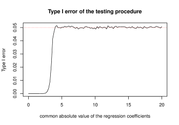
Figure 7: Type I error of the testing procedure as a function of $\|\beta\|_{\infty}$. Each point from this plot is obtained via $10^{5}$ Monte-Carlo experiments. Theoretically, under the null hypothesis and when $\|\beta\|_{\infty}$ is infinitely large, the type I error is controlled at level $\eta=0.05$. This curve corroborates this fact. Moreover, it seems the type I error is controlled at level $\eta=0.05$ for any value of $\|\beta\|_{\infty}\geq 0$.

References

- Akaike [1974] H. Akaike, A new look at the statistical model identification, IEEE Transactions on Automatic Control 19 (1974) 716–723.
- Schwarz [1978] G. Schwarz, Estimating the dimension of a model, Ann. Statist. 6 (1978) 461–464.
- Foster and George [1994] D. Foster, E. George, The risk inflation criterion for multiple regression, Ann. Stat. 22 (1994) 1947–1975.
- Bogdan et al. [2004] M. Bogdan, J. Ghosh, R. Doerge, Modifying the schwarz bayesian information criterion to locate multiple interacting quantitative trait loci, Genetics 167 (2004) 989–999.
- Chen and Chen [2008] J. Chen, Z. Chen, Extended Bayesian Information criteria for model selection with large model spaces., Biometrika 95 (2008) 759–771.
- Hoerl and Kennard [1970a] A. E. Hoerl, R. W. Kennard, Ridge regression: Biased estimation for nonorthogonal problems, Technometrics 12 (1970a) 55–67.
- Hoerl and Kennard [1970b] A. E. Hoerl, R. W. Kennard, Ridge regression: Applications to nonorthogonal problems, Technometrics 12 (1970b) 69–82.
- Chen and Donoho [1994] S. Chen, D. Donoho, Basis pursuit, in: Proceedings of 1994 28th Asilomar Conference on Signals, Systems and Computers, volume 1, 1994, pp. 41–44 vol.1. doi:10.1109/ACSSC.1994.471413.
- Tibshirani [1996] R. Tibshirani, Regression shrinkage and selection via the lasso, J. Roy. Statist. Soc. Ser. B 58 (1996) 267–288.
- Vaiter et al. [2015] S. Vaiter, M. Golbabaee, J. Fadili, G. Peyré, Model selection with low complexity priors, Inf. Inference 4 (2015) 230–287. URL: https://doi.org/10.1093/imaiai/iav005. doi:10.1093/imaiai/iav005.
- Osborne et al. [2000] M. R. Osborne, B. Presnell, B. A. Turlach, On the LASSO and its dual, J. Comput. Graph. Statist. 9 (2000) 319–337.
- Tibshirani [2013] R. J. Tibshirani, The lasso problem and uniqueness, Electron. J. Stat. 7 (2013) 1456–1490. URL: https://doi.org/10.1214/13-EJS815. doi:10.1214/13-EJS815.
- Bondell and Reich [2009] H. D. Bondell, B. J. Reich, Simultaneous factor selection and collapsing levels in anova, Biometrics 65 (2009) 169–177.
- Garcia-Donato and Paulo [2021] G. Garcia-Donato, R. Paulo, Variable selection in the presence of factors: a model selection perspective, J. Amer. Statist. Assoc. (2021). doi:10.1080/01621459.2021.1889565.
- Maj-Kańska et al. [2015] A. Maj-Kańska, P. Pokarowski, A. Prochenka, Delete or merge regressors for linear model selection, Electron. J. Stat. 9 (2015) 1749–1778.
- Pauger and Wagner [2019] D. Pauger, H. Wagner, Bayesian effect fusion for categorical predictors, Bayesian Analysis 14 (2019) 341–369.
- Stokell et al. [2021] B. G. Stokell, R. D. Shah, R. J. Tibshirani, Modelling high-dimensional categorical data using nonconvex fusion penalties, J. R. Stat. Soc. Ser. B. Stat. Methodol. 83 (2021) 579–611.
- Goodfellow et al. [2016] I. Goodfellow, Y. Bengio, A. Courville, Deep Learning, MIT Press, 2016.
- Bogdan et al. [2013] M. Bogdan, E. Van Den Berg, W. Su, E. J. Candès, Statistical estimation and testing via the sorted l1 norm, arXiv preprint arXiv:1310.1969 (2013).
- Bogdan et al. [2015] M. Bogdan, E. van den Berg, C. Sabatti, W. Su, E. J. Candès, SLOPE—adaptive variable selection via convex optimization, Ann. Appl. Stat. 9 (2015) 1103–1140. URL: https://doi.org/10.1214/15-AOAS842. doi:10.1214/15-AOAS842.
- Zeng and Figueiredo [2014] X. Zeng, M. A. T. Figueiredo, Decreasing weighted sorted regularization, IEEE Signal Processing Lett. 21 (2014) 1240–1244. doi:10.1109/LSP.2014.2331977.
- Brzyski et al. [2017] D. Brzyski, C. Peterson, P. Sobczyk, E. Candès, M. Bogdan, C. Sabatti, Controlling the rate of gwas false discoveries, Genetics 205 (2017) 61–75.
- Brzyski et al. [2019] D. Brzyski, A. Gossmann, W. Su, M. Bogdan, Group SLOPE—adaptive selection of groups of predictors, J. Amer. Statist. Assoc. 114 (2019) 419–433. URL: https://doi.org/10.1080/01621459.2017.1411269. doi:10.1080/01621459.2017.1411269.
- Kos and Bogdan [2020] M. Kos, M. Bogdan, On the asymptotic properties of SLOPE, Sankhya A 82 (2020) 499–532. URL: https://doi.org/10.1007/s13171-020-00212-5. doi:10.1007/s13171-020-00212-5.
- Abramovich and Grinshtein [2019] F. Abramovich, V. Grinshtein, High-dimensional classification by sparse logistic regression, IEEE Trans. Inform. Theory 65 (2019) 3068–3079. URL: https://doi.org/10.1109/TIT.2018.2884963. doi:10.1109/TIT.2018.2884963.
- Bellec et al. [2018] P. C. Bellec, G. Lecué, A. B. Tsybakov, Slope meets Lasso: improved oracle bounds and optimality, Ann. Statist. 46 (2018) 3603–3642. URL: https://doi.org/10.1214/17-AOS1670. doi:10.1214/17-AOS1670.
- Su and Candès [2016] W. Su, E. Candès, SLOPE is adaptive to unknown sparsity and asymptotically minimax, Ann. Statist. 44 (2016) 1038–1068. URL: https://doi.org/10.1214/15-AOS1397. doi:10.1214/15-AOS1397.
- Bondell and Reich [2008] H. D. Bondell, B. J. Reich, Simultaneous regression shrinkage, variable selection, and supervised clustering of predictors with OSCAR, Biometrics 64 (2008) 115–123, 322–323. URL: https://doi.org/10.1111/j.1541-0420.2007.00843.x. doi:10.1111/j.1541-0420.2007.00843.x.
- Sharma et al. [2013] D. B. Sharma, H. D. Bondell, H. H. Zhang, Consistent group identification and variable selection in regression with correlated predictors, J. Comput. Graph. Statist. 22 (2013) 319–340.
- Kremer et al. [2020] P. J. Kremer, S. Lee, M. Bogdan, S. Paterlini, Sparse portfolio selection via the sorted -norm, Journal of Banking & Finance 110 (2020) 105687.
- Figueiredo and Nowak [2016] M. Figueiredo, R. Nowak, Ordered weighted l1 regularized regression with strongly correlated covariates: Theoretical aspects, in: A. Gretton, C. C. Robert (Eds.), Proceedings of the 19th International Conference on Artificial Intelligence and Statistics, volume 51 of Proceedings of Machine Learning Research, PMLR, Cadiz, Spain, 2016, pp. 930–938.
- Kremer et al. [2022] P. J. Kremer, D. Brzyski, M. Bogdan, S. Paterlini, Sparse index clones via the sorted -Norm, Quant. Finance 22 (2022) 349–366.
- Skalski et al. [2022] T. Skalski, P. Graczyk, B. Kołodziejek, M. Wilczyński, Pattern recovery and signal denoising by slope when the design matrix is orthogonal, Probability and Mathematical Statistics 42 (2022) 283–302.
- Tibshirani et al. [2005] R. Tibshirani, M. Saunders, S. Rosset, J. Zhu, K. Knight, Sparsity and smoothness via the fused lasso, J. R. Stat. Soc. Ser. B Stat. Methodol. 67 (2005) 91–108.
- Schneider and Tardivel [2022] U. Schneider, P. Tardivel, The Geometry of Uniqueness, Sparsity and Clustering in Penalized Estimation, J. Mach. Learn. Res. 23 (2022) 1–36.
- Fuchs [2004] J.-J. Fuchs, On sparse representations in arbitrary redundant bases, IEEE Trans. Inform. Theory 50 (2004) 1341–1344.
- Meinshausen and Bühlmann [2006] N. Meinshausen, P. Bühlmann, High-dimensional graphs and variable selection with the lasso, Ann. Statist. 34 (2006) 1436–1462.
- Wainwright [2009] M. J. Wainwright, Sharp thresholds for high-dimensional and noisy sparsity recovery using -constrained quadratic programming (Lasso), IEEE Trans. Inform. Theory 55 (2009) 2183–2202.
- Zhao and Yu [2006] P. Zhao, B. Yu, On model selection consistency of Lasso, J. Mach. Learn. Res. 7 (2006) 2541–2563.
- Zou [2006] H. Zou, The adaptive lasso and its oracle properties, J. Amer. Statist. Assoc. 101 (2006) 1418–1429. URL: https://doi.org/10.1198/016214506000000735. doi:10.1198/016214506000000735.
- Negrinho and Martins [2014] R. Negrinho, A. Martins, Orbit regularization, in: Z. Ghahramani, M. Welling, C. Cortes, N. Lawrence, K. Weinberger (Eds.), Advances in Neural Information Processing Systems, volume 27, Curran Associates, Inc., 2014, pp. 3221–3229. URL: https://proceedings.neurips.cc/paper/2014/file/f670ef5d2d6bdf8f29450a970494dd64-Paper.pdf.
- Hiriart-Urruty and Lemaréchal [2004] J.-B. Hiriart-Urruty, C. Lemaréchal, Fundamentals of convex analysis, Springer Science & Business Media, 2004.
- Dupuis and Tardivel [2022] X. Dupuis, P. J. C. Tardivel, Proximal operator for the sorted norm: application to testing procedures based on SLOPE, J. Statist. Plann. Inference 221 (2022) 1–8.
- Tardivel et al. [2020] P. J. Tardivel, R. Servien, D. Concordet, Simple expressions of the LASSO and SLOPE estimators in low-dimension, Statistics 54 (2020) 340–352.
- Ben-Israel and Greville [2003] A. Ben-Israel, T. N. E. Greville, Generalized inverses, volume 15 of CMS Books in Mathematics/Ouvrages de Mathématiques de la SMC, second ed., Springer-Verlag, New York, 2003. Theory and applications.
- Bühlmann and Van De Geer [2011] P. Bühlmann, S. Van De Geer, Statistics for high-dimensional data: methods, theory and applications, Springer Science & Business Media, 2011.
- Tardivel et al. [2021] P. Tardivel, T. Skalski, P. Graczyk, U. Schneider, The Geometry of Model Recovery by Penalized and Thresholded Estimators, HAL preprint hal-03262087 (2021).
- Tardivel and Bogdan [2022] P. Tardivel, M. Bogdan, On the sign recovery by least absolute shrinkage and selection operator, thresholded least absolute shrinkage and selection operator, and thresholded basis pursuit denoising, Scand. J. Stat. 49 (2022) 1636–1668.
- Harter [1961] H. L. Harter, Expected values of normal order statistics, Biometrika 48 (1961) 151–165.
- Harchaoui and Lévy-Leduc [2010] Z. Harchaoui, C. Lévy-Leduc, Multiple change-point estimation with a total variation penalty, J. Amer. Statist. Assoc. 105 (2010) 1480–1493.
- Lin et al. [2017] K. Lin, J. L. Sharpnack, A. Rinaldo, R. J. Tibshirani, A sharp error analysis for the fused lasso, with application to approximate changepoint screening, in: I. Guyon, U. V. Luxburg, S. Bengio, H. Wallach, R. Fergus, S. Vishwanathan, R. Garnett (Eds.), Advances in Neural Information Processing Systems, volume 30, Curran Associates, Inc., 2017, pp. 6884–6893.
- Owrang et al. [2017] A. Owrang, M. Malek-Mohammadi, A. Proutiere, M. Jansson, Consistent change point detection for piecewise constant signals with normalized fused lasso, IEEE Signal Processing Lett. 24 (2017) 799–803.
- Qian and Jia [2016] J. Qian, J. Jia, On stepwise pattern recovery of the fused Lasso, Comput. Statist. Data Anal. 94 (2016) 221–237.
- Riccobello et al. [2022] R. Riccobello, M. Bogdan, G. Bonaccolto, P. Kremer, S. Paterlini, P. Sobczyk, Graphical modelling via the sorted l1-norm, arXiv preprint, arXiv:2204.10403 (2022).
- Højsgaard and Lauritzen [2008] S. Højsgaard, S. L. Lauritzen, Graphical Gaussian models with edge and vertex symmetries, J. R. Stat. Soc. Ser. B Stat. Methodol. 70 (2008) 1005–1027.
- Jiang et al. [2022] W. Jiang, M. Bogdan, J. Josse, S. Majewski, B. Miasojedow, V. Rockova, T. Group, Adaptive Bayesian SLOPE: Model Selection With Incomplete Data, J. Comput. Graph. Statist. 31(1) (2022) 113–137.
- Larsson et al. [2020] J. Larsson, M. Bogdan, J. Wallin, The Strong Screening Rule for SLOPE, in: H. Larochelle, M. Ranzato, R. Hadsell, M. Balcan, H. Lin (Eds.), Advances in Neural Information Processing Systems, volume 33, Curran Associates, Inc., 2020, pp. 14592–14603.
- Larsson et al. [2022] J. Larsson, Q. Klopfenstein, M. Massias, J. Wallin, Coordinate descent for SLOPE, arXiv preprint, arXiv:2210.14780 (2022) 1–12.
- Ko et al. [2007] M.-H. Ko, D.-H. Ryu, T.-S. Kim, Y.-K. Choi, A central limit theorem for general weighted sums of LNQD random variables and its application, Rocky Mountain J. Math. 37 (2007) 259–268.
- Lai and Wei [1982] T. L. Lai, C. Z. Wei, A law of the iterated logarithm for double arrays of independent random variables with applications to regression and time series models, Ann. Probab. 10 (1982) 320–335.
- Stadtmüller [1984] U. Stadtmüller, A note on the law of iterated logarithm for weighted sums of random variables, Ann. Probab. 12 (1984) 35–44.
- Cuzick [1995] J. Cuzick, A strong law for weighted sums of i.i.d. random variables, J. Theoret. Probab. 8 (1995) 625–641.