Time-domain Generalization of Kron Reduction

Abstract

Kron reduction is a network-reduction method that eliminates nodes with zero current injections from electrical networks operating in sinusoidal steady state. In the time domain, the state-of-the-art application of Kron reduction has been in networks with transmission lines that have constant $R/L$ ratios. This paper considers $RL$ networks without such restriction and puts forth a provably exact time-domain generalization of Kron reduction. Exemplifying empirical tests on a $\mathbin{\leavevmode\hbox to6.52pt{\vbox to7.78pt{\text{[drawing]}}}}-\Delta$ network are provided to validate the analytical results.

I Introduction

Complex electrical networks are encountered in several engineering domains from integrated circuits to power grids. Oftentimes, a subset of nodes in such networks feature no actuation or sensing; henceforth referred to as interior nodes. To facilitate analysis and computation, it is desirable to eliminate interior nodes and obtain reduced network models that exclusively retain the extant boundary nodes. The workhorse enabling reduction of electrical networks derives from the classical Kron reduction [1]. A familiar example of this is the elemental wye-delta ($\mathbin{\leavevmode\hbox to6.52pt{\vbox to7.78pt{\text{[drawing]}}}}$-$\Delta$) transform. (See Fig. 1.) The method is well defined when all excitations are in sinusoidal steady state and all network interconnections are modeled as impedances at a fixed frequency. Kron reduction in such a setting boils down to computing a Schur complement of the admittance matrix (that establishes the algebraic map between nodal voltages and current injections). The effort [2] provides a comprehensive survey of Kron reduction and establishes connections to a wide range of graph- and system-theoretic constructs; similarly [3, 4] highlight some recent extensions for diverse applications.

Interestingly, Kron reduction is not as widely studied in the time domain with arbitrary excitation, wherein the governing dynamics are differential-algebraic equations (DAEs). Exact model-reduction results in these settings are restricted to homogeneous networks, which assume lines to have constant $R/L$ ratios, and include purely resistive and inductive networks as special cases [5, 6]. Attempts to address generalized settings yield limited accuracy guarantees [7].

Pursuing a time-domain generalization of Kron reduction, this work considers an $RL$ network without the restrictive constant $R/L$ constraint. For the considered setting, this work contributes a projection-based generalized time-domain reduced model with two prominent advantages: i) the reduction is exact, implying equivalence to the full-order model; and ii) the time-domain analysis permits inclusion of arbitrary initial conditions (as opposed to frequency-domain approaches). Phasor-domain Kron reduction and time-domain Kron reduction with constant $R/L$ ratios are recovered as special cases.

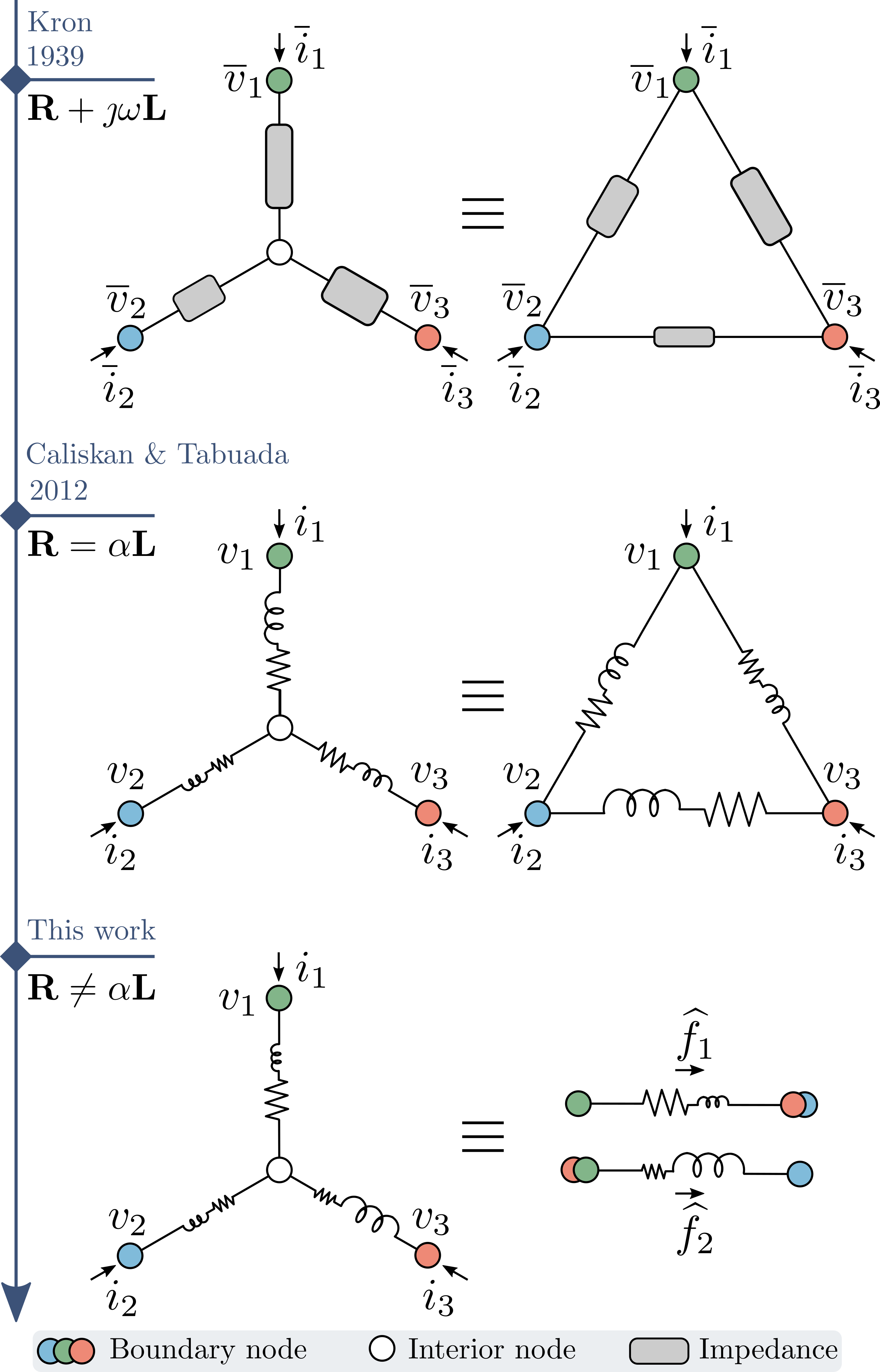
Figure 1: Prominent existing results and proposed advancement towards electrical network reduction. State-of-the art for phasor domain is the classical Kron reduction (top); that in the time domain is restricted to networks with constant $R/L$ ratios (middle). We provide a generalization in the time domain (bottom) that recovers prior results as special cases.

II Preliminaries

II-A Phasor Representation

In sinusoidal steady state at frequency $\omega$, we express time-domain signals as $x(t)=|x|\cos(\omega t+\theta_{x})$, where $(|x|,\theta_{x})$ are constants. For analytical ease, we represent $x(t)$ by a corresponding complex-valued rotating vector

$$\overrightarrow{x}(t)=x(t)+\jmath x(t-\nicefrac{{\pi}}{{2\omega}})=|x|\mathrm{e}^{\jmath\theta_{x}}\mathrm{e}^{\jmath\omega t}=\overline{x}\mathrm{e}^{\jmath\omega t}.$$

The complex constant quantity $\overline{x}=|x|\mathrm{e}^{\jmath\theta_{x}}$ is referred to as a phasor. Dynamics satisfied by real-valued signals $x(t)$ in a linear and time-invariant system are also satisfied by $\overrightarrow{x}(t)$. This facilitates translating differential equations in $x(t)$ to algebraic equations in $\overline{x}$ and underscores the popularity of phasors in steady-state analysis of electrical networks.

II-B Electrical-network Model

Consider a single-phase $RL$ network described by a connected graph $\mathcal{G}=(\mathcal{N},\mathcal{E})$. The node set is indexed as $\mathcal{N}=\{1,\dots,N\}$, and let $E=|\mathcal{E}|$. Arbitrarily assigning directions, an edge $e$ from node $m$ to $n$ is denoted as $e=(m,n)$. Line resistances and inductances for an edge $e\in\mathcal{E}$ are denoted by $r_{e},\leavevmode\nobreak\ \ell_{e}\geq 0$. The topology of $\mathcal{G}$ is captured by the incidence matrix $\mathbf{B}\in\{0,\pm 1\}^{N\times E}$ with entries $B_{k,e}=1(-1)$ if $k=m(n)$ when $\exists\leavevmode\nobreak\ e=(m,n)\in\mathcal{E}$; and $B_{k,e}=0$, otherwise.

Let the real-valued signals $v_{n}(t)$ and $i_{n}(t)$ denote the instantaneous voltage and current injection at node $n$; and $f_{e}(t)$ represent current flow on edge $e$. In what follows, the explicit time dependence of signals will be omitted for notational ease. For all lines $e=(m,n)$, the line currents and node voltages obey the first-order $RL$-dynamics

$$\ell_{e}\dot{f}_{e}+r_{e}f_{e}=v_{m}-v_{n}.$$ (1)

The model in (1) requires $\ell_{e}\neq 0$ to retain dynamics. Otherwise, the flows can be trivially expressed in terms of the node voltages. Thus, the following non-prohibitive assumption is made at the outset to facilitate exposition.

Assumption 1.

For all edges $e\in\mathcal{E}$, inductance $\ell_{e}>0$.

Define the vectors $\mathbf{v}=\{v_{n}\}_{n\in\mathcal{N}}$, $\mathbf{i}=\{i_{n}\}_{n\in\mathcal{N}}$, and $\mathbf{f}=\{f_{e}\}_{e\in\mathcal{E}}$. Collectively, line dynamics in (1), along with Kirchoff’s current law (KCL) can be succinctly written using matrix-vector notation as

$$\mathbf{L}\dot{\mathbf{f}} =-\mathbf{R}\mathbf{f}+\mathbf{B}^{\top}\mathbf{v},$$ (2a)

$$\mathbf{i} =\mathbf{B}\mathbf{f},$$ (2b)

where $\mathbf{R}=\operatorname{diag}(\{r_{e}\}_{e\in\mathcal{E}})$ and $\mathbf{L}=\operatorname{diag}(\{\ell_{e}\}_{e\in\mathcal{E}})$. This paper focuses on the dynamical system in (2), identifying: input $\mathbf{v}$, state $\mathbf{f}$, and output $\mathbf{i}$. (While this work considers a voltage-actuated network with currents serving as outputs, the developed approach can be extended to settings with current actuation and voltage outputs.) Since $\mathbf{L}$ is invertible per Assumption 1, the model (2) constitutes an ordinary differential equation (ODE) with a linear output equation.

II-C Problem Statement

Suppose the network graph $\mathcal{G}$ has $N_{0}\geq 1$ interior nodes collected in the set $\mathcal{N}_{0}\subset\mathcal{N}$. Without loss of generality, the network nodes can be numbered to feature the boundary nodes first, thereby enabling the partitioning $\mathbf{i}=[\mathbf{i}_{1}^{\top}\leavevmode\nobreak\ \mathbf{i}_{0}^{\top}]^{\top}$ and $\mathbf{v}=[\mathbf{v}_{1}^{\top}\leavevmode\nobreak\ \mathbf{v}_{0}^{\top}]^{\top}$. Corresponding to the interior nodes $\mathcal{N}_{0}$, we have $\mathbf{i}_{0}=\boldsymbol{0}$. To explicitly impose zero-current injection for the nodes in $\mathcal{N}_{0}$, let us partition the incidence matrix as $\mathbf{B}^{\top}=[\mathbf{B}^{\top}_{1}\leavevmode\nobreak\ \mathbf{B}^{\top}_{0}]$, where $\mathbf{B}^{\top}_{0}$ has $N_{0}$ columns. The ensuing dynamical system is now governed by the DAE

$$\mathbf{L}\dot{\mathbf{f}} =-\mathbf{R}\mathbf{f}+\mathbf{B}^{\top}\mathbf{v},$$ (3a)

$$\boldsymbol{0} =\mathbf{B}_{0}\mathbf{f},$$ (3b)

with the corresponding output equation

$$\mathbf{i}_{1}=\mathbf{B}_{1}\mathbf{f}.$$ (4)

In a nutshell, Kron reduction aspires to uncover the link between current injections $\mathbf{i}_{1}$ and voltages $\mathbf{v}_{1}$. Our effort is to do so by reducing the DAE (3) to an ODE with inputs being exclusively the voltages $\mathbf{v}_{1}$. Before we present this result, we overview prior efforts.

III Prior Model-reduction Results

III-A Kron Reduction in Steady State

Consider a steady-state operating condition, wherein flows, injections, and nodal voltages are in sinusoidal steady state with frequency $\omega$. In line with the discussion in Section II for steady-state analysis, let us denote the complex-valued rotating vectors for current flow, injection, and nodal voltages by $\overrightarrow{\mathbf{f}},\overrightarrow{\mathbf{i}},\overrightarrow{\mathbf{v}}$, and recognize that they satisfy (2). Substituting $\overrightarrow{\mathbf{f}}=\overline{\mathbf{f}}\mathrm{e}^{\jmath\omega t}$, $\overrightarrow{\mathbf{i}}=\overline{\mathbf{i}}\mathrm{e}^{\jmath\omega t}$, and $\overrightarrow{\mathbf{v}}=\overline{\mathbf{v}}\mathrm{e}^{\jmath\omega t}$ yields:

$$\jmath\omega\mathbf{L}\overline{\mathbf{f}}\mathrm{e}^{\jmath\omega t} =-\mathbf{R}\overline{\mathbf{f}}\mathrm{e}^{\jmath\omega t}+\mathbf{B}^{\top}\overline{\mathbf{v}}\mathrm{e}^{\jmath\omega t},$$ (5a)

$$\overline{\mathbf{i}}\mathrm{e}^{\jmath\omega t} =\mathbf{B}\overline{\mathbf{f}}\mathrm{e}^{\jmath\omega t}.$$ (5b)

Solving for $\overline{\mathbf{f}}$ from (5a) and substituting the resultant in (5b) yields the familiar algebraic network model

$$\overline{\mathbf{i}}=\mathbf{B}(\mathbf{R}+\jmath\omega\mathbf{L})^{-1}\mathbf{B}^{\top}\overline{\mathbf{v}}=\mathbf{Y}\overline{\mathbf{v}},$$ (6)

where $\mathbf{Y}=\mathbf{B}(\mathbf{R}+\jmath\omega\mathbf{L})^{-1}\mathbf{B}^{\top}$ is the admittance matrix. The inverse $(\mathbf{R}+\jmath\omega\mathbf{L})^{-1}$ exists owing to the invertibility of $\mathbf{L}$ per Assumption 1 and non-negativity of resistances $r_{e}\geq 0,\,\forall e\in\mathcal{E}$. Suitably partitioning (6) provides

$$\begin{bmatrix}\overline{\mathbf{i}}_{1}\\ \mathbf{0}\end{bmatrix}=\begin{bmatrix}\mathbf{Y}_{11}&\mathbf{Y}_{10}\\ \mathbf{Y}_{10}^{\top}&\mathbf{Y}_{00}\end{bmatrix}\begin{bmatrix}\overline{\mathbf{v}}_{1}\\ \overline{\mathbf{v}}_{0}\end{bmatrix}.$$ (7)

From the second row in (7), we can isolate $\overline{\mathbf{v}}_{0}=-\mathbf{Y}_{00}^{-1}\mathbf{Y}_{10}^{\top}\overline{\mathbf{v}}_{1}$, which, when substituted back in the first row, yields the reduced model

$$\overline{\mathbf{i}}_{1}=(\mathbf{Y}\setminus\mathbf{Y}_{00})\overline{\mathbf{v}}_{1}=\mathbf{Y}_{r}\overline{\mathbf{v}}_{1},$$ (8)

where $\mathbf{Y}_{r}=(\mathbf{Y}\setminus\mathbf{Y}_{00})=\mathbf{Y}_{11}-\mathbf{Y}_{10}\mathbf{Y}_{00}^{-1}\mathbf{Y}_{10}^{\top}$ is the Schur complement of $\mathbf{Y}_{00}$ of the admittance matrix, $\mathbf{Y}$, and is commonly referred to as the Kron-reduced admittance matrix. The Kron-reduced admittance matrix $\mathbf{Y}_{r}$ corresponds to an equivalent connected network of series impedances [2]. The previous manipulation relies on the invertibility of $\mathbf{Y}_{00}$, which is guaranteed per the result below.

Lemma 1.

Given a strict subset $\mathcal{N}_{0}\subset\mathcal{N}$, the submatrix $\mathbf{Y}_{00}$ defined as per (7) is invertible if one of the following conditions hold: c1) $r_{e}>0,\leavevmode\nobreak\ \forall e\in\mathcal{E}$; c2) $l_{e}>0,\leavevmode\nobreak\ \forall e\in\mathcal{E}$.

A proof is provided in Appendix -A. The sufficient condition c2) coincides with Assumption 1, thus ensuring applicability of Lemma 1 to the networks considered in this work.

Remark 1.

Under varying network models, results related to Lemma 1 may be found in the recent works [8, 9]. These establish invertibility for principal submatrices of $\mathbf{Y}$ under a set of conditions including c1). The furnished approaches are complicated by the presence of shunt elements and transformers, see [9]. However, for the $RL$ network considered here, the relatively simpler proof for Lemma 1 suffices.

III-B Time-domain Reduction for Homogeneous Networks

To reduce the time-domain model in (3) for eliminating the interior nodes in $\mathcal{N}_{0}$, previous results rely on the so called homogeneous network assumption, see [6]. This assumption dictates that all edges, $e\in\mathcal{E}$, have a constant $r_{e}/\ell_{e}$ ratio, translating to $\mathbf{R}=\alpha\mathbf{L}$ for some $\alpha>0$. Substituting this homogeneity condition in (3a) yields

$$\dot{\mathbf{f}}=-\alpha\mathbf{f}+\mathbf{L}^{-1}\mathbf{B}^{\top}\mathbf{v}.$$ (9)

Pre-multiplying (9) with $\mathbf{B}$ and using KCL (as transcribed in (2b)) provides the dynamic model in current injections:

$$\dot{\mathbf{i}}=-\alpha\mathbf{i}+\mathbf{B}\mathbf{L}^{-1}\mathbf{B}^{\top}\mathbf{v}=\widetilde{\mathbf{L}}\mathbf{v},$$ (10)

where $\widetilde{\mathbf{L}}=\mathbf{B}\mathbf{L}^{-1}\mathbf{B}^{\top}$. Similar to $\mathbf{Y}$ in (6), $\widetilde{\mathbf{L}}$ in (10) corresponds to a Laplacian of the graph $\mathcal{G}$. One can partition (10), use $\mathbf{i}_{0}=0$ (and hence $\dot{\mathbf{i}}_{0}=0$), to obtain

$$\begin{bmatrix}\dot{\mathbf{i}}_{1}\\ \mathbf{0}\end{bmatrix}=-\alpha\begin{bmatrix}\mathbf{i}_{1}\\ \mathbf{0}\end{bmatrix}+\begin{bmatrix}\widetilde{\mathbf{L}}_{11}&\widetilde{\mathbf{L}}_{10}\\ \widetilde{\mathbf{L}}_{10}^{\top}&\widetilde{\mathbf{L}}_{00}\end{bmatrix}\begin{bmatrix}\mathbf{v}_{1}\\ \mathbf{v}_{0}\end{bmatrix}.$$ (11)

The structure of (11) conveniently allows for elimination of the voltages $\mathbf{v}_{0}$, as was done in transiting from (7) to (8). Specifically, the equation in the second row yields $\mathbf{v}_{0}=-\widetilde{\mathbf{L}}_{00}^{-1}\widetilde{\mathbf{L}}_{10}^{\top}\mathbf{v}_{1}$, which, when substituted in the first row, yields the reduced dynamical model in terms of current injections:

$$\dot{\mathbf{i}}_{1}=-\alpha\mathbf{i}_{1}+(\widetilde{\mathbf{L}}\setminus\widetilde{\mathbf{L}}_{00})\mathbf{v}_{1}.$$ (12)

The invertibility of $\widetilde{\mathbf{L}}_{00}$ is ascertained from the following observation: The definition of $\widetilde{\mathbf{L}}$ in (10) indicates that for a purely inductive network with inductances given by $\mathbf{L}$, the related matrix $\mathbf{Y}$ can be written as $\jmath\omega\widetilde{\mathbf{L}}$; see (6). Owing to Lemma 1 and Assumption 1, the invertibility of $\mathbf{Y}_{00}$ or $\jmath\omega\widetilde{\mathbf{L}}_{00}$ (equivalently $\widetilde{\mathbf{L}}_{00}$) is guaranteed.

The above delineated steps feature resemblance to Kron reduction in (7)-(8), and the reduced model (12) admits striking network-theoretic similarities as well. Specifically, matrix $(\widetilde{\mathbf{L}}\setminus\widetilde{\mathbf{L}}_{00})$ in (12) corresponds to a Laplacian of a reduced graph, which topologically coincides with the one obtained from $\mathbf{Y}_{r}$ in (8) (see Fig. 1(middle)). The topology of the reduced network depends on the originating one, and is agnostic to the edge weights, see  [10, Prop. 5.7]. While not explicitly captured in the mathematical presentation, the previous approach applies to purely resistive/inductive networks as well.

The above approach accomplishes model reduction by transforming the states from $\mathbf{f}$ to $\mathbf{i}$, thereby applying the zero-injection condition directly on $\mathbf{i}$. However, the maneuvers involved only apply to homogeneous networks. The next section addresses a general setting.

IV Generalized Time-domain Model Reduction

This section puts forth the proposed approach to eliminate zero-injection nodes $\mathcal{N}_{0}$ from the time-domain model (3). Next, it is shown that the prior results of Section III can be obtained as special instances of our generalized approach. Subsequently, flexibilities in the reduced-model structure are elaborated and circuit interpretations are outlined.

IV-A Main Result

The $RL$ dynamics (3a) feature $E$ differential equations in $E$-length state-vector $\mathbf{f}$. However, constraint (3b) restricts the flows $\mathbf{f}$ to a low-dimensional subspace; specifically $\mathbf{f}\in\operatorname{null}(\mathbf{B}_{0})$. It is worth noting that

$$\operatorname{dim}(\operatorname{null}(\mathbf{B}_{0}))=E-N_{0},$$

where $N_{0}=|\mathcal{N}_{0}|$. (See Appendix -B for proof.) Therefore, one can obtain a low-dimensional embedding $\widehat{\mathbf{f}}\in\mathds{R}^{E-N_{0}}$ for vectors $\mathbf{f}\in\operatorname{null}(\mathbf{B}_{0})$ via

$$\mathbf{f}=\mathbf{P}\widehat{\mathbf{f}},$$ (13)

where the matrix $\mathbf{P}$ should be chosen to yield $\operatorname{range}(\mathbf{P})=\operatorname{null}(\mathbf{B}_{0})$. In a graph-theoretic sense, matrix $\mathbf{P}$ spans the space orthogonal to the cutset space defined by cuts of interior nodes in $\mathcal{N}_{0}$ [10]. Being a (potentially abstract) representation of network current flows, we refer to $\widehat{\mathbf{f}}$ as pseudoflows. Using the prescribed embedding, the ensuing result formally establishes the sought reduced model corresponding to (3).

Theorem 1.

Consider the differential equation

$$\widehat{\mathbf{L}}\dot{\widehat{\mathbf{f}}}=-\widehat{\mathbf{R}}\widehat{\mathbf{f}}+\widehat{\mathbf{B}}^{\top}\mathbf{v}_{1},$$ (14)

where, $\widehat{\mathbf{L}}=\mathbf{P}^{\top}\mathbf{L}\mathbf{P}$, $\widehat{\mathbf{R}}=\mathbf{P}^{\top}\mathbf{R}\mathbf{P}$, and $\widehat{\mathbf{B}}=\mathbf{B}_{1}\mathbf{P}$. The following hold:

• Matrix $\widehat{\mathbf{L}}$ is invertible rendering (14) an ODE.

• Solutions of network flows obtained from (14) with initial condition $\widehat{\mathbf{f}}_{0}$ alongside (13) coincide with the solutions of (3) with $\mathbf{f}(t=0)=\mathbf{P}\widehat{\mathbf{f}}_{0}$.

Proof.

We will start with establishing the invertibility of $\widehat{\mathbf{L}}$. Note that positive $\ell_{e}$’s from Assumption 1 imply $\mathbf{L}\succ 0$. Further, since columns of $\mathbf{P}$ are linearly independent, we get $\widehat{\mathbf{L}}\succ 0$. This guarantees the invertibility of $\widehat{\mathbf{L}}$, and renders (14) an ODE. Towards establishing the equivalence of (14) and (3), we substitute (13) in (3a) to obtain

$$\mathbf{L}\mathbf{P}\dot{\widehat{\mathbf{f}}}=-\mathbf{R}\mathbf{P}\widehat{\mathbf{f}}+\mathbf{B}^{\top}\mathbf{v}.$$ (15)

Equation (15) constitutes an over-determined system of $E$ differential equations with linear dependence. To eliminate the linear dependence, pre-multiply (15) with $\mathbf{P}^{\top}$ to obtain

$$\mathbf{P}^{\top}\mathbf{L}\mathbf{P}\dot{\widehat{\mathbf{f}}} =-\mathbf{P}^{\top}\mathbf{R}\mathbf{P}\widehat{\mathbf{f}}+\mathbf{P}^{\top}[\mathbf{B}_{0}^{\top}\leavevmode\nobreak\ \mathbf{B}_{1}^{\top}]\begin{bmatrix}\mathbf{v}_{0}\\ \mathbf{v}_{1}\end{bmatrix}$$

$$=-\mathbf{P}^{\top}\mathbf{R}\mathbf{P}\widehat{\mathbf{f}}+\mathbf{P}^{\top}\mathbf{B}_{1}^{\top}\mathbf{v}_{1},$$ (16)

where, the second line follows from the fact that $\operatorname{range}(\mathbf{P})=\operatorname{null}(\mathbf{B}_{0})$, or $\mathbf{B}_{0}\mathbf{P}=\boldsymbol{0}$. Substituting the definitions of $(\widehat{\mathbf{L}},\widehat{\mathbf{R}},\widehat{\mathbf{B}})$ yields (14). ∎

In line with the problem statement in Section II-C, the reduced ODE model (14) eliminates the unknown voltages $\mathbf{v}_{0}$ and features exclusively the voltages $\mathbf{v}_{1}$ as inputs. Finally, the output equation (4) gets modified using (13) to

$$\mathbf{i}_{1}=\mathbf{B}_{1}\mathbf{P}\widehat{\mathbf{f}},$$ (17)

thus yielding the sought relation from input $\mathbf{v}_{1}$ to output $\mathbf{i}_{1}$.

Remark 2 (Is $\mathbf{P}$ unique?).

Given matrix $\mathbf{B}_{0}^{\top}$, the matrix $\mathbf{P}$ featuring in the reduced model of Theorem 1 is not unique. It can be built by collecting as columns, an arbitrary basis for $\operatorname{null}(\mathbf{B}_{0})$. Technical details on choice of a specific $\mathbf{P}$ and related interpretations are provided in Section IV-C.

Remark 3 (Relation to Galerkin Projection).

The proposed approach features similarities to the Galerkin projection-based model order reduction (PMOR) [11]. In applying Galerkin PMOR to get a reduced model of order $M<N$ for (3), one seeks a matrix $\mathbf{V}\in\mathds{R}^{E\times M}$, such that $\mathbf{f}\approx\mathbf{V}\widehat{\mathbf{f}}$, where $\widehat{\mathbf{f}}\in\mathds{R}^{M}$. Substituting this subspace approximation in (3a) yields $\mathbf{L}\mathbf{V}\dot{\widehat{\mathbf{f}}}=-\mathbf{R}\mathbf{V}\widehat{\mathbf{f}}+\mathbf{B}^{\top}\mathbf{v}+\mathbf{r}_{1}$, with residual $\mathbf{r}_{1}$ capturing the approximation error. Next, one pre-multiplies the previous equation by $\mathbf{V}^{\top}$ while imposing $\mathbf{V}^{\top}\mathbf{r}_{1}=\boldsymbol{0}$ towards reducing the error; thus obtaining a reduced $M$-order model. The accuracy loss from reduction is quantified by $\|\mathbf{r}_{1}\|$. While the approach of Theorem 1 is similar in spirit to Galerkin PMOR, unlike the later, it attains an equivalent reduced model with no approximation error. Specifically, with the choice of reduced-model order $M=N-E_{0}$, we make the subspace approximation exact in (13) with $\mathbf{V}=\mathbf{P}$; which on substitution in (3) yields $\|\mathbf{r}_{1}\|=0$.

IV-B Prior Results as Special Cases

This section reconciles the prior results (8) and (12) with the proposed generalized reduced model (14). To this end, we first evaluate the reduced models yielded by Theorem 1 for the two special cases of Section III. Next we will show that these models coincide with (8) and (12).

IV-B1 Steady-state model

Assigning the steady-state form to pseudoflows as $\overline{\widehat{\mathbf{f}}}\mathrm{e}^{\jmath\omega t}$ and substituting in (14) yields (after some elementary algebraic manipulations) $(\widehat{\mathbf{R}}+\jmath\omega\widehat{\mathbf{L}})\overline{\widehat{\mathbf{f}}}=\widehat{\mathbf{B}}\bar{\mathbf{v}}_{1}$. Subsequently using $\overline{\mathbf{f}}=\mathbf{P}\overline{\widehat{\mathbf{f}}}$ and $\overline{\mathbf{i}}_{1}=\mathbf{B}_{1}\overline{\mathbf{f}}$, from (4) and (13) applied to steady-state values, one gets

$$\overline{\mathbf{i}}_{1}=\mathbf{B}_{1}\mathbf{P}\big{(}\mathbf{P}^{\top}(\mathbf{R}+\jmath\omega\mathbf{L})\mathbf{P}\big{)}^{-1}\mathbf{P}^{\top}\mathbf{B}_{1}^{\top}\overline{\mathbf{v}}_{1},$$ (18)

where the definitions of $(\widehat{\mathbf{L}},\widehat{\mathbf{R}},\widehat{\mathbf{B}})$ follow from Theorem 1.

IV-B2 Homogeneous networks

Substituting the homogeneous-network condition $\mathbf{R}=\alpha\mathbf{L}$, or equivalently $\widehat{\mathbf{R}}=\alpha\widehat{\mathbf{L}}$, in (14) and premultipying by $\widehat{\mathbf{L}}^{-1}$ provides

$$\dot{\widehat{\mathbf{f}}}=-\alpha\widehat{\mathbf{f}}+\widehat{\mathbf{L}}^{-1}\widehat{\mathbf{B}}^{\top}\mathbf{v}_{1}.$$

Further, premultiplying by $\mathbf{B}_{1}\mathbf{P}$ (invoking (4) and (13)), and substituting the definitions of $(\widehat{\mathbf{L}},\widehat{\mathbf{B}})$ yields

$$\dot{\mathbf{i}}_{1}=-\alpha\mathbf{i}_{1}+\mathbf{B}_{1}\mathbf{P}(\mathbf{P}^{\top}\mathbf{L}\mathbf{P})^{-1}\mathbf{P}^{\top}\mathbf{B}_{1}^{\top}\mathbf{v}_{1}.$$ (19)

Next, we show the equivalence of the reduced models (18) and (19) to prior results (8) and (12) in two steps. First, we note that (18) and (19) feature matrix $\mathbf{P}$, which is not unique. Hence, we provide an algebraic claim in Lemma 2 to eliminate the apparent ambiguity from the non-uniqueness of $\mathbf{P}$. Second, we show in Proposition 1 that via appropriate instantiation of a weighting matrix, the models in (18) and (19) coincide with the prior results (8) and (12). The proof of Proposition 1 builds upon the technical Lemma 2.

Lemma 2.

For a connected graph $(\mathcal{N},\mathcal{E})$, consider complex-valued edge weights $w_{e}\neq 0,\forall e\in\mathcal{E}$, and a row-block partition of the companion incidence matrix as $\mathbf{B}^{\top}=[\mathbf{B}^{\top}_{1}\leavevmode\nobreak\ \mathbf{B}^{\top}_{0}]$; define $\mathbf{W}=\operatorname{diag}(\{w_{e}\}_{e\in\mathcal{E}})$. Given a full-column-rank matrix $\mathbf{P}$ with $\operatorname{range}(\mathbf{P})=\operatorname{null}(\mathbf{B}_{0})$, it holds that

$$\begin{split}\mathbf{P}(\mathbf{P}^{\top}\mathbf{W}\mathbf{P})^{-1}\mathbf{P}^{\top}&=\\ \mathbf{W}^{-1}-\mathbf{W}^{-1}&\mathbf{B}_{0}^{\top}(\mathbf{B}_{0}\mathbf{W}^{-1}\mathbf{B}_{0}^{\top})^{-1}\mathbf{B}_{0}\mathbf{W}^{-1}.\end{split}$$ (20)

Proof.

Define $\widetilde{\mathbf{B}}_{0}=\mathbf{B}_{0}\mathbf{W}^{-\frac{1}{2}}$ and $\widetilde{\mathbf{P}}=\mathbf{W}^{\frac{1}{2}}\mathbf{P}$. Given ${\operatorname{range}(\mathbf{P})=\operatorname{null}(\mathbf{B}_{0})}$, it follows that $\operatorname{range}(\widetilde{\mathbf{P}})=\operatorname{null}(\widetilde{\mathbf{B}}_{0})$ and the LHS of (20) can be written as

$$\mathbf{P}(\mathbf{P}^{\top}\mathbf{W}\mathbf{P})^{-1}\mathbf{P}^{\top}=\mathbf{W}^{-\frac{1}{2}}\underbrace{\widetilde{\mathbf{P}}(\widetilde{\mathbf{P}}^{\top}\widetilde{\mathbf{P}})^{-1}\widetilde{\mathbf{P}}^{\top}}_{=\mathds{P}_{\widetilde{\mathbf{P}}}}\mathbf{W}^{-\frac{1}{2}},$$ (21)

where $\mathds{P}_{\widetilde{\mathbf{P}}}$ denotes the projection onto $\operatorname{range}(\widetilde{\mathbf{P}})$ (in this case, equivalent to the projection onto $\operatorname{null}(\widetilde{\mathbf{B}}_{0})$). Denote the projection onto $\operatorname{range}(\widetilde{\mathbf{B}}_{0}^{\top})$ as $\mathds{P}_{\widetilde{\mathbf{B}}_{0}^{\top}}=\widetilde{\mathbf{B}}_{0}^{\top}(\widetilde{\mathbf{B}}_{0}\widetilde{\mathbf{B}}_{0}^{\top})^{-1}\widetilde{\mathbf{B}}_{0}$, where the invertibility of $\widetilde{\mathbf{B}}_{0}\widetilde{\mathbf{B}}_{0}^{\top}=\mathbf{B}_{0}\mathbf{W}^{-1}\mathbf{B}_{0}^{\top}$ is guaranteed since $\mathbf{B}_{0}$ is a strict row partition of the incidence matrix of a connected graph, and hence features linearly independent rows. Using $\operatorname{null}(\widetilde{\mathbf{B}}_{0})=\operatorname{range}(\widetilde{\mathbf{B}}_{0}^{\top})$, it can be shown that

$$\mathds{P}_{\widetilde{\mathbf{P}}}=\mathds{I}-\mathds{P}_{\widetilde{\mathbf{B}}_{0}^{\top}},$$ (22)

where $\mathds{I}$ is the identity matrix of size $E$. Pre- and post-multiplying (22) with $\mathbf{W}^{-\frac{1}{2}}$ and substituting the definitions of $(\mathds{P}_{\widetilde{\mathbf{P}}},\mathds{P}_{\widetilde{\mathbf{B}}_{0}^{\top}})$ provides

$$\begin{split}\mathbf{W}^{-\frac{1}{2}}\widetilde{\mathbf{P}}(\widetilde{\mathbf{P}}^{\top}\widetilde{\mathbf{P}})^{-1}\widetilde{\mathbf{P}}^{\top}\mathbf{W}^{-\frac{1}{2}}&=\\ \mathbf{W}^{-1}-\mathbf{W}^{-\frac{1}{2}}&\widetilde{\mathbf{B}}_{0}^{\top}(\widetilde{\mathbf{B}}_{0}\widetilde{\mathbf{B}}_{0}^{\top})^{-1}\widetilde{\mathbf{B}}_{0}\mathbf{W}^{-\frac{1}{2}}.\end{split}$$ (23)

Substituting $\widetilde{\mathbf{B}}_{0}=\mathbf{B}_{0}\mathbf{W}^{-\frac{1}{2}}$ and $\widetilde{\mathbf{P}}=\mathbf{W}^{\frac{1}{2}}\mathbf{P}$ above yields (20) and completes the proof. ∎

Lemma 2 establishes that despite the non-uniqueness of $\mathbf{P}$, the structural form in the LHS of (20) equals the unique matrix in the RHS. The next result, proved in Appendix -C, uses Lemma 2 to reconcile (18) to (8), and (19) to (12).

Proposition 1.

For the complex edge weights $\{w_{e}\}$ introduced in Lemma 2, define Laplacian matrix $\widetilde{\mathbf{W}}=\mathbf{B}\mathbf{W}^{-1}\mathbf{B}^{\top}$, and let $\widetilde{\mathbf{W}}_{00}$ be the matrix block partition corresponding to the interior nodes $\mathcal{N}_{0}$. Then, it holds that

$$\mathbf{B}_{1}\mathbf{P}(\mathbf{P}^{\top}\mathbf{W}\mathbf{P})^{-1}\mathbf{P}^{\top}\mathbf{B}_{1}^{\top}=\widetilde{\mathbf{W}}\setminus\widetilde{\mathbf{W}}_{00}.$$ (24)

Choosing $\mathbf{W}=\mathbf{R}+\jmath\omega\mathbf{L}$ in (24) establishes the equivalence of (18) and (8); and choosing $\mathbf{W}=\mathbf{L}$ establishes the equivalence of (19) and (12).

IV-C Choices of $\mathbf{P}$ and Related Interpretations

1. Given the flows on all-but-one edges incident on an interior node, one can trivially recover the extant flow via KCL. Thus, a sub-vector $\widehat{\mathbf{f}}$ built by omitting from $\mathbf{f}$, one incident-edge flow per interior node can serve as a reduced representation. Hence, one can express $\mathbf{f}=\mathbf{P}\widehat{\mathbf{f}}$ by stacking the rows of $\mathbf{P}$ as suitable canonical vectors corresponding to the retained flows; and as $\{0,\pm 1\}$ vectors to calculate the omitted flows.

2. Compute the basis vectors spanning $\operatorname{null}{(\mathbf{B}_{0})}$. Stack these as columns to obtain $\mathbf{P}$.

3. One can choose $\mathbf{P}$ to yield diagonal $(\widehat{\mathbf{L}},\leavevmode\nobreak\ \widehat{\mathbf{R}})$ via the following steps: i) Compute a matrix $\mathbf{P}^{\prime}$ to span $\operatorname{null}{(\mathbf{B}_{0}^{\top})}$ as described in choice 2); ii) Set $\widehat{\mathbf{L}}^{\prime}=\mathbf{P}^{\prime\top}\mathbf{L}\mathbf{P}^{\prime}$ and $\widehat{\mathbf{R}}^{\prime}=\mathbf{P}^{\prime\top}\mathbf{R}\mathbf{P}^{\prime}$; iii) Obtain the generalized eigen-value decomposition $\widehat{\mathbf{L}}^{\prime}\mathbf{V}=\widehat{\mathbf{R}}^{\prime}\mathbf{V}\mathbf{D}$; and iv) set $\mathbf{P}=\mathbf{P}^{\prime}\mathbf{V}$. It can be verified that thus-obtained $\mathbf{P}$ yields diagonal $(\widehat{\mathbf{L}},\leavevmode\nobreak\ \widehat{\mathbf{R}})$ with non-negative entries. The latter stems from using $\mathbf{L},\mathbf{R}\succeq 0$ in the definitions of $\widehat{\mathbf{L}},\widehat{\mathbf{R}}$. The reduced model (14) can then be interpreted as $(E-N_{0})$ independent $RL$-circuits actuated by a linear combination of voltages in $\mathbf{v}_{1}$; see Fig. 1(bottom). The individual equations read as

   $$\widehat{L}_{kk}\dot{\hat{f}}_{k}+\widehat{R}_{kk}\hat{f}_{k}=\sum_{n=1}^{N-N_{0}}\beta_{kn}v_{n},$$

   where $\beta_{kn}$’s are entries of the product $\mathbf{P}^{\top}\mathbf{B}_{1}^{\top}$.

V Numerical Tests

This section empirically illustrates the effectiveness of the proposed generalization using $\mathbin{\leavevmode\hbox to6.52pt{\vbox to7.78pt{\text{[drawing]}}}}$-$\Delta$ transformation as an example. For comparison, we adopt a baseline approach from  [7] that heuristically extends Kron reduction to the time domain. Denoted as $(\mathcal{B})$, the approach involves the following steps: $(\mathrm{S}1)$ Given a $\mathbin{\leavevmode\hbox to6.52pt{\vbox to7.78pt{\text{[drawing]}}}}$-connected $RL$ network with one interior node (see Fig. 1), choose a frequency $\omega_{0}$ and build an admittance matrix per (6) that corresponds to a $\mathbin{\leavevmode\hbox to6.52pt{\vbox to7.78pt{\text{[drawing]}}}}$-connected impedance network. $(\mathrm{S}2)$ Obtain a reduced $\Delta$-connected impedance network using (8). $(\mathrm{S}3)$ Separate out real and imaginary parts of impedances in the reduced $\Delta$ connection and factor out $\omega_{0}$ to recover a $\Delta$-connected $RL$ network. Clearly, $(\mathcal{B})$ lacks a theoretical claim of equivalence in the time domain; it is further accompanied by two implementation ambiguities: $(\mathrm{A}1)$ To obtain a time-domain solution of the $\mathbin{\leavevmode\hbox to6.52pt{\vbox to7.78pt{\text{[drawing]}}}}$-connected $RL$ network, one would be presented with the initial conditions $\mathbf{f}^{\mathbin{\leavevmode\hbox to4.56pt{\vbox to5.45pt{\text{[drawing]}}}}}_{0}\in\mathds{R}^{3\times 1}$. On obtaining the $\Delta$-connected $RL$ network in $(\mathrm{S}3)$, how does one obtain a corresponding $\mathbf{f}^{\Delta}_{0}$? $(\mathrm{A}2)$ How to choose $\omega_{0}$ in $(\mathrm{S}1)$ when the network may be actuated by arbitrary voltages?

V-A Setup

Two sets of numerical tests will be presented next to compare our approach, $(\mathcal{B})$, and a ground-truth DAE model implemented in the Matlab-Simulink environment. Both are conducted for a $\mathbin{\leavevmode\hbox to6.52pt{\vbox to7.78pt{\text{[drawing]}}}}$-connected $RL$ network with $RL$ parameters randomly drawn from $[0.5,1]$, and given by $\mathbf{R}=\operatorname{diag}([0.98\leavevmode\nobreak\ 0.99\leavevmode\nobreak\ 0.58])\leavevmode\nobreak\ \Omega$ and $\mathbf{L}=\operatorname{diag}([0.55\leavevmode\nobreak\ 0.64\leavevmode\nobreak\ 0.77])\leavevmode\nobreak\ \mathrm{H}$; and initial branch currents $\mathbf{f}^{\mathbin{\leavevmode\hbox to4.56pt{\vbox to5.45pt{\text{[drawing]}}}}}_{0}=-[5,5,-10]^{\top}\leavevmode\nobreak\ \mathrm{A}$. To obtain an initial condition for the current flows $\mathbf{f}^{\Delta}_{0}$ given $\mathbf{f}^{\mathbin{\leavevmode\hbox to4.56pt{\vbox to5.45pt{\text{[drawing]}}}}}_{0}$ in $(\mathcal{B})$, we have to ensure the boundary-node current injections agree in both $\Delta$ and $\mathbin{\leavevmode\hbox to6.52pt{\vbox to7.78pt{\text{[drawing]}}}}$ representations. One such solution, $\tilde{\mathbf{f}}^{\Delta}_{0}$ can be obtained using Matlab command lsqminnorm$(\mathbf{B}_{r},\mathbf{f}^{\mathbin{\leavevmode\hbox to4.56pt{\vbox to5.45pt{\text{[drawing]}}}}}_{0})$, where $\mathbf{B}_{r}$ is the incidence matrix of the $\Delta$ connection. This operation returns a minimum-norm solution to $\mathbf{B}_{r}\mathbf{f}^{\Delta}_{0}=\mathbf{f}^{\mathbin{\leavevmode\hbox to4.56pt{\vbox to5.45pt{\text{[drawing]}}}}}_{0}$. With cyclic edge direction assignment in the $\Delta$ connection, we have $\mathbf{B}_{r}\mathbf{1}=\boldsymbol{0}$; hence for any scalar $\gamma$, vector $\tilde{\mathbf{f}}^{\Delta}_{0}+\gamma\mathbf{1}$ conforms with the required initial-current injections. Given the ambiguity, $5$ random instances of $\gamma$ are drawn uniformly from $[-5,5]\leavevmode\nobreak\ \mathrm{A}$ in our execution of $(\mathcal{B})$.

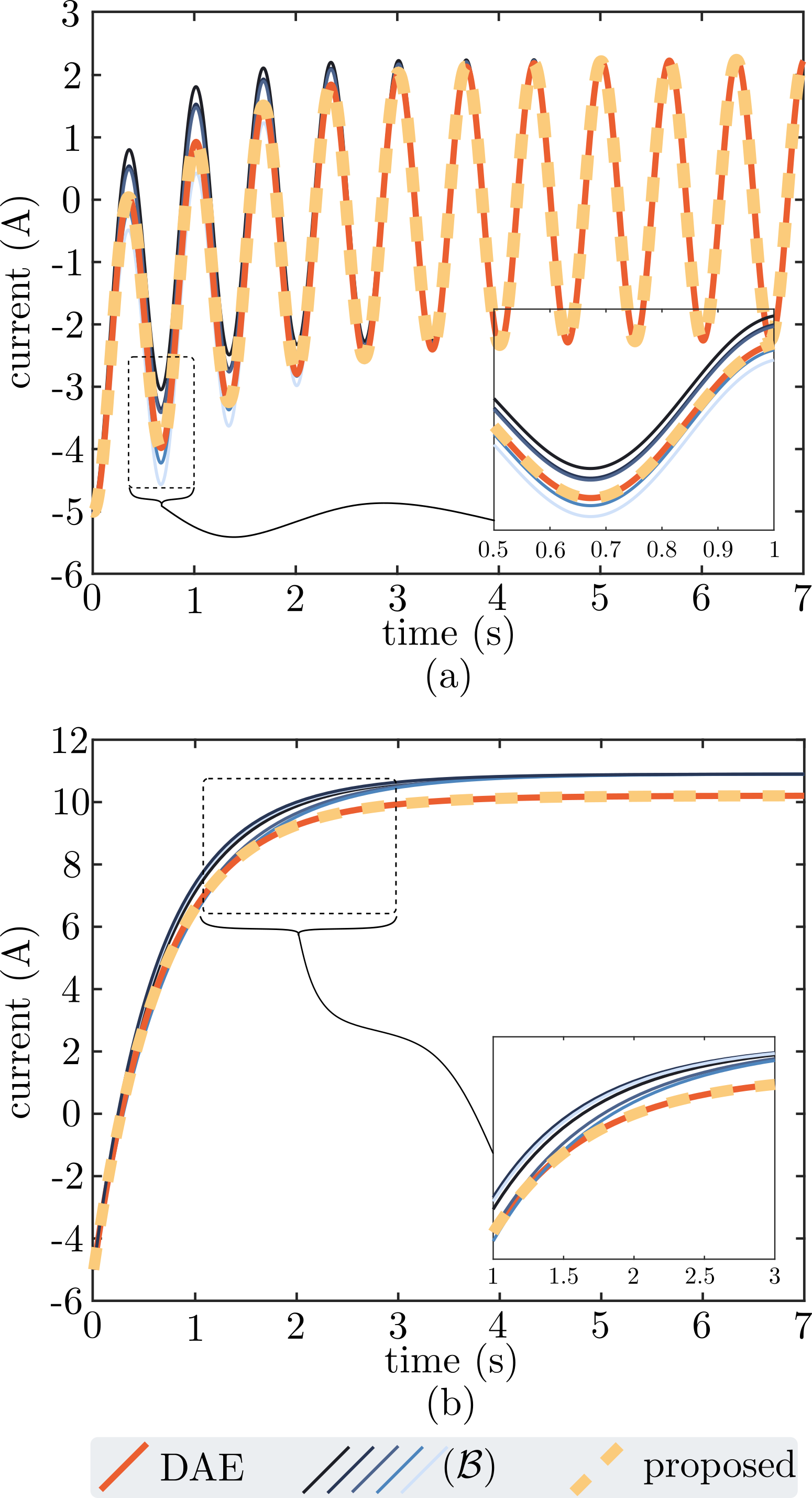
Figure 2: Current injections $i_{1}(t)$ obtained with: a) sinusoidal-voltage excitation; and b) step-voltage excitation.

V-B Results & Inferences

In the first set of tests, we apply $1.5\leavevmode\nobreak\ \mathrm{Hz}$ sinusoidal voltages with amplitudes $120\leavevmode\nobreak\ \mathrm{V}$ and phases $(0,30^{\circ},-30^{\circ})$ to the three boundary nodes. To implement our approach, $\mathbf{P}$ was obtained using Matlab command null$(\mathbf{A}_{0})$, the initial condition for simulating the proposed reduced model (14) was evaluated from (13). To implement $(\mathcal{B})$, $\omega_{0}$ was picked to be $2\pi\times 1.5\leavevmode\nobreak\ \mathrm{rad}\cdot\mathrm{s}^{-1}$. The current injections at node $1$, $i_{1}(t)$, obtained via the three approaches are illustrated in Fig. 2(a). The following observations are in order: i) the initial values for all approaches coincide by design; ii) results from the reduced model obtained with the proposed approach coincide point wise with the ground-truth DAE model; and iii) results from $(\mathcal{B})$ with randomized initializations vary during transient conditions but align with the ground-truth DAE model in steady state (aligning with the claims in [7]).

In the next set of tests, the excitation voltages were changed to be step functions assuming steady-state values $[120,100,110]^{\top}\leavevmode\nobreak\ \mathrm{V}$. The current injections at node $1$, $i_{1}(t)$, obtained via the three approaches are illustrated in Fig. 2(b). One observes that: i) results from the reduced model obtained with the proposed approach coincide point wise with the ground-truth DAE model; and ii) results of $(\mathcal{B})$ with randomized initializations coincide with each other in steady state, but all are different from the ground-truth.

These sets of numerical tests demonstrate that while the proposed model reduction holds for arbitrary voltage-actuated $RL$ networks in the time domain, an attempt to heuristically extend the classical Kron reduction may not yield accurate results (even in steady state).

VI Concluding Remarks

This work put forth a time-domain generalization of Kron reduction for $RL$ networks. Prominent prior results for steady-state conditions and homogeneous networks were shown to be special instances of the proposed model. Numerical tests on the well-known $\mathbin{\leavevmode\hbox to6.52pt{\vbox to7.78pt{\text{[drawing]}}}}-\Delta$ transformation setup validated the approach and highlighted the limitations of existing heuristics. Given that the projection matrix $\mathbf{P}$ relates to the cut-set space of the underlying graph, it is tempting to further investigate graph-theoretic interpretations of the proposed low-dimensional embedding.

-A Proof of Lemma 1

Having $r_{e},\leavevmode\nobreak\ \ell_{e}\geq 0$ entails $\Re(\mathbf{Y})$ and $\Im(\mathbf{Y})$ are positive semidefinite; implying $\Re(\mathbf{Y}_{00}),\leavevmode\nobreak\ \Im(\mathbf{Y}_{00})\succeq 0$. Next, we prove the invertibility of $\mathbf{Y}_{00}$ assuming condition c1) is satisfied. The proof for c2) follows similarly. Given $r_{e}>0\leavevmode\nobreak\ \forall e$, the matrix $\Re(\mathbf{Y})$ is a Laplacian matrix. Furthermore, matrix $\Re(\mathbf{Y}_{00})$ is a strict principal submatrix of $\Re(\mathbf{Y})$ as $\mathcal{N}_{0}\subset\mathcal{N}$; hence $\Re(\mathbf{Y}_{00})\succ 0$. Proving by contradiction, let us assume that the matrix $\mathbf{Y}_{00}$ is singular, implying $\exists\leavevmode\nobreak\ \mathbf{x}=\mathbf{x}_{r}+\jmath\mathbf{x}_{i}\neq\boldsymbol{0}$ such that $\mathbf{Y}_{00}\mathbf{x}=\boldsymbol{0}$. Separating the real and imaginary parts of $\mathbf{Y}_{00}\mathbf{x}=\boldsymbol{0}$ reads

$$\Re(\mathbf{Y}_{00})\mathbf{x}_{r}-\Im(\mathbf{Y}_{00})\mathbf{x}_{i}=\boldsymbol{0},$$ (25a)

$$\Im(\mathbf{Y}_{00})\mathbf{x}_{r}+\Re(\mathbf{Y}_{00})\mathbf{x}_{i}=\boldsymbol{0}.$$ (25b)

Since $\Re(\mathbf{Y}_{00})\succ 0$, (25a) yields

$$\mathbf{x}_{r}=[\Re(\mathbf{Y}_{00})]^{-1}\Im(\mathbf{Y}_{00})\mathbf{x}_{i}.$$ (26)

Substituting $\mathbf{x}_{r}$ from (26) in (25b) yields

$$\left(\Im(\mathbf{Y}_{00})[\Re(\mathbf{Y}_{00})]^{-1}\Im(\mathbf{Y}_{00})+\Re(\mathbf{Y}_{00})\right)\mathbf{x}_{i}=\boldsymbol{0}.$$ (27)

Using $\Im(\mathbf{Y}_{00})\succeq 0$, $\Re(\mathbf{Y}_{00})\succ 0$, one finds $\left(\Im(\mathbf{Y}_{00})[\Re(\mathbf{Y}_{00})]^{-1}\Im(\mathbf{Y}_{00})+\Re(\mathbf{Y}_{00})\right)$ is invertible, implying $\mathbf{x}_{i}=\boldsymbol{0}$ from (27). Further, (26) yields $\mathbf{x}_{r}=\boldsymbol{0}$, or $\mathbf{x}=\boldsymbol{0}$, leading to a contradiction; thus, $\mathbf{Y}_{00}$ is invertible.

-B Proof for $\operatorname{dim}(\operatorname{null}(\mathbf{B}_{0}))=E-N_{0}$

Since $\mathbf{B}$ is the incidence matrix of a connected graph, it features $N-1$ linearly independent rows with $\mathbf{1}^{\top}\mathbf{B}=\boldsymbol{0}$. Thus, any selection of $N_{0}<N$ rows are linearly independent. Hence, the rows of matrix $\mathbf{B}_{0}$ are linearly independent implying the dimension of $\operatorname{null}(\mathbf{B}_{0})$ is $E-N_{0}$.

-C Proof of Proposition 1

From the definition $\widetilde{\mathbf{W}}=\mathbf{B}\mathbf{W}^{-1}\mathbf{B}^{\top}$, and the partition $\mathbf{B}^{\top}=[\mathbf{B}^{\top}_{1}\leavevmode\nobreak\ \mathbf{B}^{\top}_{0}]$, matrix $\widetilde{\mathbf{W}}$ can be expressed as

$$\widetilde{\mathbf{W}}=\begin{bmatrix}\widetilde{\mathbf{W}}_{11}&\widetilde{\mathbf{W}}_{10}\\ \widetilde{\mathbf{W}}_{10}^{\top}&\widetilde{\mathbf{W}}_{00}\end{bmatrix} =\begin{bmatrix}\mathbf{B}_{1}\\ \mathbf{B}_{0}\end{bmatrix}\mathbf{W}^{-1}[\mathbf{B}_{1}^{\top}\leavevmode\nobreak\ \leavevmode\nobreak\ \mathbf{B}_{0}^{\top}]$$

$$=\begin{bmatrix}\mathbf{B}_{1}\mathbf{W}^{-1}\mathbf{B}_{1}^{\top}&\mathbf{B}_{1}\mathbf{W}^{-1}\mathbf{B}_{0}^{\top}\\ \mathbf{B}_{0}\mathbf{W}^{-1}\mathbf{B}_{1}^{\top}&\mathbf{B}_{0}\mathbf{W}^{-1}\mathbf{B}_{0}^{\top}\end{bmatrix}.$$

The Schur complement $\widetilde{\mathbf{W}}\setminus\widetilde{\mathbf{W}}_{00}$ is given by

$$\widetilde{\mathbf{W}}\setminus\widetilde{\mathbf{W}}_{00}=\widetilde{\mathbf{W}}_{11}-\widetilde{\mathbf{W}}_{10}\widetilde{\mathbf{W}}_{00}^{-1}\widetilde{\mathbf{W}}_{10}^{\top}$$

$$=\mathbf{B}_{1}\mathbf{W}^{-1}\mathbf{B}_{1}^{\top}-\mathbf{B}_{1}\mathbf{W}^{-1}\mathbf{B}_{0}^{\top}(\mathbf{B}_{0}\mathbf{W}^{-1}\mathbf{B}_{0}^{\top})^{-1}\mathbf{B}_{0}\mathbf{W}^{-1}\mathbf{B}_{1}^{\top}$$

$$=\mathbf{B}_{1}\big{(}\mathbf{P}(\mathbf{P}^{\top}\mathbf{W}\mathbf{P})^{-1}\mathbf{P}^{\top}\big{)}\mathbf{B}_{1}^{\top},$$

where, the second equality follows from substituting the matrix blocks, and the last equality follows from Lemma 2.

References

• [1] G. Kron, Tensor Analysis of Networks.   Hoboken, NJ, USA: Wiley, 1939.
• [2] F. Dörfler and F. Bullo, “Kron reduction of graphs with applications to electrical networks,” IEEE Trans. Circuits Syst. I, vol. 60, no. 1, pp. 150–163, 2013.
• [3] S. V. Dhople, B. B. Johnson, F. Dörfler, and A. O. Hamadeh, “Synchronization of nonlinear circuits in dynamic electrical networks with general topologies,” IEEE Trans. Circuits Syst. I, vol. 61, no. 9, pp. 2677–2690, 2014.
• [4] N. Monshizadeh, C. De Persis, A. J. van der Schaft, and J. M. A. Scherpen, “A novel reduced model for electrical networks with constant power loads,” IEEE Trans. Autom. Contr., vol. 63, no. 5, pp. 1288–1299, 2018.
• [5] S. Y. Caliskan and P. Tabuada, “Kron reduction of power networks with lossy and dynamic transmission lines,” in Proc. IEEE Conf. on Decision and Control, Maui, HI, 2012, pp. 5554–5559.
• [6] ——, “Towards Kron reduction of generalized electrical networks,” Automatica, vol. 50, no. 10, pp. 2586–2590, 2014.
• [7] A. Floriduz, M. Tucci, S. Riverso, and G. Ferrari-Trecate, “Approximate Kron reduction methods for electrical networks with applications to plug-and-play control of AC islanded microgrids,” IEEE Trans. Contr. Syst. Technol., vol. 27, no. 6, pp. 2403–2416, 2019.
• [8] A. M. Kettner and M. Paolone, “On the properties of the power systems nodal admittance matrix,” IEEE Trans. Power Syst., vol. 33, no. 1, pp. 1130–1131, 2018.
• [9] D. Turizo and D. K. Molzahn, “Invertibility conditions for the admittance matrices of balanced power systems,” arXiv preprint arXiv:2012.04087, 2020.
• [10] F. Dörfler, J. W. Simpson-Porco, and F. Bullo, “Electrical networks and algebraic graph theory: Models, properties, and applications,” Proc. IEEE, vol. 106, no. 5, pp. 977–1005, 2018.
• [11] A. C. Antoulas, C. A. Beattie, and S. Güğercin, Interpolatory methods for model reduction.   Philadelphia, PA, USA: SIAM, 2020.