Effective Seed Scheduling for Fuzzing with
Graph Centrality Analysis

Abstract

Seed scheduling, the order in which seeds are selected, can greatly affect the performance of a fuzzer. Existing approaches schedule seeds based on their historical mutation data, but ignore the structure of the underlying Control Flow Graph (CFG). Examining the CFG can help seed scheduling by revealing the potential edge coverage gain from mutating a seed.

An ideal strategy will schedule seeds based on a count of all reachable and feasible edges from a seed through mutations, but computing feasibility along all edges is prohibitively expensive. Therefore, a seed scheduling strategy must approximate this count. We observe that an approximate count should have 3 properties —(i) it should increase if there are more edges reachable from a seed; (ii) it should decrease if mutation history information suggests an edge is hard to reach or is located far away from currently visited edges; and (iii) it should be efficient to compute over large CFGs.

We observe that centrality measures from graph analysis naturally provide these three properties and therefore can efficiently approximate the likelihood of reaching unvisited edges by mutating a seed. We therefore build a graph called the edge horizon graph that connects seeds to their closest unvisited nodes and compute the seed node’s centrality to measure the potential edge coverage gain from mutating a seed.

We implement our approach in K-Scheduler and compare with many popular seed scheduling strategies. We find that K-Scheduler increases feature coverage by 25.89% compared to Entropic and edge coverage by 4.21% compared to the next-best AFL-based seed scheduler, in arithmetic mean on 12 Google FuzzBench programs. It also finds 3 more previously-unknown bugs than the next-best AFL-based seed scheduler.

I Introduction

Fuzzing is a popular security testing technique that has found numerous vulnerabilities in real-world programs [46, 6, 15, 20, 13, 35, 37, 55, 59, 52, 64, 55]. Fuzzers automatically search through the input space of a program for specific inputs that result in potentially exploitable buggy behaviors. However, the input spaces of most real-world programs are too large to explore exhaustively. Therefore, most existing fuzzers follow an edge-coverage-guided evolutionary approach for guiding the input generation process to ensure that the generated inputs explore different control flow edges of the target program [62, 3, 2]. Starting from a seed input corpus, a coverage-guided fuzzer repeatedly selects a seed from the corpus, mutates it, and adds only those mutated inputs back to the corpus that generate new edge coverage. The performance of such fuzzers have been shown to heavily depend on seed scheduling, the order in which the seeds are selected for mutation [28].

The main challenge in seed scheduling is to identify which seeds in a corpus, when mutated, are more likely to explore many new edges. Performing more mutations on such promising seeds can achieve higher edge coverage. Most prior work on seed scheduling identifies and prioritizes the promising seeds based on the historical distribution of edge/path coverage across prior mutations of the seeds. For example, a fuzzer can prioritize the seeds whose mutations, in the past, resulted in a higher path coverage [60] or triggered rarer edges [32]. However, these existing approaches ignore the structure of the underlying Control Flow Graph (CFG). For example, consider a seed s1 whose execution path is close to many unvisited edges and a seed s2 whose execution path is close to only one unvisited edge. Existing coverage-guided fuzzers might schedule seed S2 before S1 based on historical patterns. However, examining the structure of the CFG will reveal that S1 is indeed more promising than S2 as mutating it can potentially result in exploration of many unvisited edges that are close to the S1’s execution path.

The naive strategy of scheduling seeds simply based on the counts of all potentially reachable edges in the CFG for each seed is unlikely to be effective. Such a naive approach assumes that all CFG edges are equally likely to be reachable through mutations which does not hold true for most real-world programs. In fact, some shallow edges tend to be reachable by a large number of mutated inputs while other deep edges are only reached by a few, if any at all (as many branches might be infeasible) [40]. An ideal strategy would schedule seeds based on the count of all reachable and feasible edges from a seed by mutations. The seeds with higher edge counts will be mutated more. However, computing the feasibility along all edges is impractical as it will incur prohibitive computational cost.

Therefore, a seed scheduling strategy must approximate the feasible edge count. We observe that such an approximation should have 3 properties. First, the approximate count should increase if there are many edges reachable from a seed. Second, the count should decrease if mutation history information suggests that an edge is hard to reach or is located far away from currently visited edges. Empirical evidence from prior work has shown that reaching child nodes through input mutations is typically harder than reaching parent nodes [40] because the number of inputs that can reach a child, for a given path, is strictly less than or equal to the number of inputs that can reach the parent. Third, the approximate count must be efficient to compute for large CFGs as real-world CFGs can be quite large (e.g., inter-procedural CFGs might contain thousands of nodes).

Our key observation is that centrality measures from graph influence analysis naturally provide the aforementioned properties while measuring a node’s influence on the graph. Influence analysis is often used to identify a graph’s (e.g., a social network’s) most influential nodes and graph centrality measures each node’s influence on other nodes with three properties as described below. First, centrality measures additively scale up a node’s influence proportional to the number of edges that are reachable from the node. Each sequence of edges of the same length is treated equally independent of its order. Second, centrality measures can easily incorporate external contribution (e.g., based on past mutation history) to a node’s influence and can decay contributions from farther away nodes to the node’s influence. Contributions decay multiplicatively with the increase in distance (i.e., more intermediate nodes) to reduce contributions from longer paths. Finally, centrality can be efficiently approximated on large graphs using iterative methods [29].

In this paper, we introduce a new approach for seed scheduling based on centrality analysis of the seeds on the CFG. We prioritize scheduling seeds with the largest centrality, i.e., approximate counts of unvisited but potentially reachable CFG edges from a seed through mutations. To measure a seed’s influence with centrality, we modify the CFG to construct an edge horizon graph containing the eponymous horizon nodes. The horizon nodes form the boundary between the visited and unvisited regions of the CFG for a given fuzzing corpus.

Since horizon nodes delineate between the visited and unvisited regions of the CFG, we first classify CFG nodes as visited or unvisited based on the coverage of a fuzzer’s current corpus. We then define horizon nodes as unvisited nodes with a visited parent node. These nodes are crucial to fuzzing because a fuzzer must first visit a horizon node before going further into the unvisited region of the CFG. The centrality of horizon nodes reachable by mutations on a seed therefore measures the seed’s ability to discover new edge coverage. Hence, we introduce one node corresponding to each seed and connect the nodes to their corresponding horizon nodes. We do not keep any visited node in the edge horizon graph to avoid inflating a seed’s centrality score with contributions from already visited nodes.

To compute centrality over the edge horizon graph, we use Katz centrality because it provides all the three desired approximation properties described earlier in this section and can operate on directed graphs like CFGs. We also use historical mutation data to bias the influence of horizon nodes to a value between 0 and 1 where values closer to 0 mean the node is harder to reach by mutations. The bias value estimates the hardness to reach a node by counting how many mutations reach a node’s parents but fail to reach the node itself. Using the centrality scores for all seeds, a fuzzer can prioritize the seed with the highest centrality. We also periodically re-compute the edge horizon graph and centrality scores during a fuzzing campaign.

We implement our centrality-analysis-based seed scheduling technique as part of K-Scheduler (K stands for Katz centrality). Our evaluation shows that K-Scheduler increases feature coverage by 25.89% compared to Entropic and edge coverage by 4.21% compared to the next-best AFL-based seed scheduler, in arithmetic mean on 12 Google FuzzBench programs. It also finds 3 more previously-unknown bugs than the next-best AFL-based seed scheduler. We also conduct preliminary experiments to show the utility of K-Scheduler in non-fuzzing seed scheduling settings such as concolic execution and measure the impact of K-Scheduler’s design choices. Our main contributions are described below:

• We model seed scheduling in fuzzing as a graph centrality analysis problem.

• We construct an edge horizon graph and use Katz centrality to compute centrality scores that approximate the number of reachable and feasible unvisited CFG edges from a seed.

• We implement our approach in K-Scheduler and integrate it into Libfuzzer and AFL to show the generic utility of our approach. We release our implementation on https://github.com/Dongdongshe/K-Scheduler.

• We demonstrate that using K-Scheduler increases feature coverage by 25.89% compared to Entropic and edge coverage by 4.21% compared to the next-best AFL-based seed scheduler, in arithmetic mean on 12 Google FuzzBench programs. It also finds 3 more previously-unknown bugs than the next-best AFL-based seed scheduler.

II Graph Influence Analysis Background

II-A Centrality Measures for Influence Analysis

Identifying a graph’s most influential nodes is a common and important task in graph analysis. Many different centrality measures exist in the literature to estimate a node’s influence [39]. For example, degree centrality measures a node’s influence by counting its direct neighbors. This technique can identify a node with local influence over its neighbors. Eigenvector centrality, in contrast, can identify nodes with global influence over the entire graph. However, eigenvector centrality can fail to produce useful scores on directed graphs [36, 38]. Because program CFGs are directed graphs and we want to measure the global influence of a node to reach other nodes in a graph, we use Katz centrality, a variant of eigenvector centrality for directed graphs. We believe that Pagerank centrality, another eigenvector centrality variant, is not suitable for our setting because it dilutes node influence by the number of its direct neighbors. Such artificial dilutions will undesirably decrease a node’s influence in a program’s CFG. We conduct experiments to experimentally support this claim in Section VI.

For directed graphs like a program CFG, a node’s neighbors can be defined by incoming or outgoing edges. Therefore, centrality measures are classified as out-degree if they use outgoing edges or in-degree if they use incoming edges during the computation. Their actual usage depend on the target domain. For example, academic citation graphs use in-degree centrality measures because influential papers are highly cited. In our setting, we use out-degree Katz centrality because we want to measure a node’s ability to reach as many unvisited CFG edges (with respect to the current fuzzing corpus) as possible. We describe the details of the out-degree Katz centrality measure below.

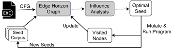
Figure 1: Fuzzer workflow with K-Scheduler.

II-B Katz Centrality

⬇ 1 2a, b=read_input(); 3if(a > 20){ 4 return 1; 5} 6else if(a > 10){ 7 if (b > 20) 8 return 2; 9 else if (b > 10) 10 return 3; 11 else 12 return 4; 13} 14else 15 return 5;

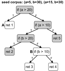
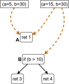
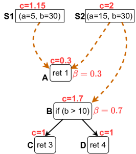
(a) Program CFG. (b) Edge horizon graph (c) Computing Katz Centrality

Figure 2: This figure shows how K-Scheduler is used for seed scheduling on a small program. Given the code example on the left, Figure 2a shows the corresponding CFG, colored as gray if a node is visited and white if unvisited based on the fuzzer corpus. Figure 2b shows the edge horizon graph. Figure 2c displays node Katz centrality scores computed by iterative power method illustrated in Table I. A fuzzer will prioritize seed $(\texttt{a}=15,\texttt{b}=30)$ because it has the highest centrality score.

Let $A$ denote an $n$ by $n$ adjacency matrix of a graph with $n$ nodes. If there is an edge connecting node i to node j, element $A_{ij}=1$. Otherwise, $A_{ij}=0$. Let $\mathbf{c}$ denote the Katz centrality vector of size $n$. The element corresponding to node $i$, $c_{i}$, is defined as follows,

$$c_{i}=\alpha\sum_{j=1}^{n}A_{ij}c_{j}+\beta_{i}$$ (1)

where $\alpha\in[0,1]$ and $\beta_{i}$ is the i-th element of $\bm{\beta}$, a vector of size $n$ consisting of non-negative elements. Conceptually, the left equation term captures that node centrality additively depends on its neighbors centrality and assigns each neighbor equal weight. Because the sum operator is commutative, the centrality score is independent of the order in which nodes are reached. The right term $\bm{\beta}$ captures the minimum centrality of a node, which we will later use in Section IV to bias the centrality of horizon nodes based on historical mutation data. The $\alpha$ term represents the decay factor, so that long paths are weighted less than short paths as we show in Section IV.

In matrix form, equation 1 can be written as

$$\mathbf{c}=\alpha A\mathbf{c}+\bm{\beta}$$ (2)

To compute $\mathbf{c}$, the Katz centrality vector, one can solve the linear system so that

$$\mathbf{c}=(I-\alpha A)^{-1}\bm{\beta}$$ (3)

However, computing the matrix inverse in Equation 3 is prohibitively expensive with $O(n^{3})$ complexity for large graphs. In practice, an iterative approach called the power method is used to approximate $\mathbf{c}$ based on Equation 2. After initially setting $\mathbf{c}(0)=\mathbf{\beta}$, the power method computes the t-th iteration with the following formula,

$$\mathbf{c}(t)=\alpha A\mathbf{c}(t-1)+\bm{\beta}$$ (4)

where $\mathbf{c}(t)$ denotes the t-th iteration. Each iteration increases the power of matrix $A$ which corresponds to considering neighbors farther away. Hence, Katz centrality measures global node influence over the entire graph. Each iteration also reduces the contribution of farther away nodes to a node’s influence as we describe in Section IV. The power method converges to the centrality vector in Equation 3 with $O(n)$ complexity under some reasonable assumptions about the graph topology [38] such as $\alpha$ having to be less than the multiplicative inverse of the largest eigenvalue. We refer the reader to [36, 38] for more technical details.

III Overview of Our Approach

Workflow. Figure 1 depicts the workflow of K-Scheduler. Given a program, seed corpus, and a target program’s inter-procedural CFG, we modify the CFG to produce an edge horizon graph composed of only seed, horizon, and non-horizon unvisited nodes. We then use Katz centrality to perform centrality analysis on the edge horizon graph. A fuzzer prioritizes the seed with the highest centrality score. As a fuzzer’s mutations reach previously unvisited nodes, we delete these newly visited nodes and re-compute Katz centrality on the updated edge horizon graph.

Motivating Example. Figure 2 shows a motivating example to explain our approach. The sample program (shown on the left) returns different values based on user input stored in variables a and b. Intuitively, we want to pick the seed node that can reach as many unvisited CFG edges as possible. In this case, this corresponds to seed node $(\texttt{a}=15,\texttt{b}=30)$. To do this, our approach K-Scheduler takes two steps.

Edge Horizon Graph. First, we modify the CFG to build the edge horizon graph. We classify nodes in the program’s CFG as visited or unvisited based on the coverage of a fuzzer’s current corpus. Figure 2a shows a classification of program’s CFG nodes, where nodes in gray are visited and nodes in white are unvisited. We next identify horizon nodes, which border the visited and unvisited CFG. In Figure 2a, the horizon nodes are nodes A and B since they are unvisited nodes with a visited parent node. We then insert seed nodes into the CFG and connect them to any horizon node whose parent is visited along the seed’s execution path. For example, seed $(\texttt{a}=5,\texttt{b}=30)$ takes both $False$ sides of the branch and hence its horizon node is node A. We connect this seed node to horizon node A. Finally, we delete all visited nodes in the CFG. Figure 2b shows the resulting edge horizon graph.

Katz centrality. Second, we compute Katz centrality over the edge horizon graph. We use the $\beta$ parameter in the centrality computation to estimate the hardness to reach a node by mutations. For this example, we assume that out of 100 mutations, $70$ reached the parent of horizon node A, so its $\beta=1-\frac{70}{100}=0.3$ and 30 reached the parent of horizon node $B$, so its $\beta=1-\frac{30}{100}=0.7$. This shows that horizon node A is harder to reach by mutations because a fuzzer failed to reach it with $70\%$ of its mutations. The remaining nodes default to $\beta=1$ as described in Section IV. Katz centrality also decays the contribution from further away nodes when computing a node’s centrality with an $\alpha$ parameter. For this example, we assume $\alpha=0.5$.

TABLE I: Katz centrality computation by the iterative power method for the edge horizon graph in Figure 2c. Each row corresponds to a node’s centrality value and each column indicates the current iteration. The power method converges in 3 steps on this simple graph. Assume $\alpha=0.5$ and $\mathbf{\beta}=\mathbf{c}(0)$.

	t=0	t=1	t=2	t=3
$c_{a}$	0.3	0.3	0.3	0.3
$c_{b}$	0.7	1.7	1.7	1.7
$c_{c}$	1	1	1	1
$c_{d}$	1	1	1	1
$c_{s1}$	1	1.15	1.15	1.15
$c_{s2}$	1	1.5	2	2

Detailed Katz centrality computation. To see how Katz centrality is computed by the power method from Section II, we show $\mathbf{c}(t=0),\mathbf{c}(t=1),...$ until it converges when $t=3$ in Table I, where the rows indicate the centrality score for a node and the columns indicate time. To explain the intuition behind Katz centrality, we walk through the iteration for a single seed node s2 to explain the computation. Initially, $c_{s2}(0)=1$. Using Equation 4 from Section II, $c_{s2}(1)=\alpha(c_{a}(0)+c_{b}(0))+\beta_{s2}=0.5*(0.3+0.7)+1=1.5$. Then, the next iteration is $c_{s2}(2)=\alpha(c_{a}(1)+c_{b}(1))+\beta_{s2}=0.5*(0.3+1.7)+1=2$ and $c_{s2}(3)=c_{s2}(2)$ due to convergence. This computation illustrates how Katz centrality decays contributions from further away nodes. The number of edges reachable from s2 is 4 but its Katz centrality score is 2 due to this decay. Moreover, the computation reflects that Katz centrality increases if there are more edges reachable from a node. Compared to s2, s1 can only reach 1 edge and hence its centrality of $1.15$ is lower. Based on the results of Katz centrality, a fuzzer will prioritize seed $(\texttt{a}=15,\texttt{b}=30)$ because it has the highest centrality score among seed nodes.

IV Methodology

In this section, we detail our approach to seed selection with influence analysis. We first describe how we build an edge horizon graph from a program’s CFG and then how we compute Katz centrality on the edge horizon graph. Lastly, we describe how our approach can be integrated into a coverage-guided fuzzer.

IV-A Edge Horizon Graph Construction

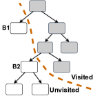
Figure 3: A target program’s CFG with visited nodes colored in gray and unvisited nodes colored white. The dashed-brown line shows the boundary between the visited and unvisited regions of the CFG. Horizon nodes B1 and B2 sit at the border and are defined as unvisited nodes with a visited parent node.

We construct the target program’s directed inter-procedural control-flow graph $CFG=(N,E)$, where $N$ is the set of nodes representing the basic blocks and $E$ is the set of edges capturing control-flow transitions through branches, jumps, etc. In the rest of the paper, for clarity, we use CFG to refer to the inter-procedural CFG unless otherwise noted.

Algorithm 1 Edge Horizon Graph Construction.

Input:	$G$ $\leftarrow$ Inter-procedural CFG
	$S$ $\leftarrow$ Seed corpus
	$P$ $\leftarrow$ Program

1:/* Classify Nodes as Visited/Unvisited */

2:$V,U=\{\},\{\}$

3:for $s\in S$ do

4:    $visited\_nodes=$ GetCoverage$(P,s)$

5:    $V=V\cup visited\_nodes$ $\triangleright$ Union $visited\_nodes$ with $V$

6:$U=G.nodes\setminus V$ $\triangleright$ Compute the complement set of $V$

7:

8:/* Identify Horizon Nodes */

9:$H=\{\}$

10:for $u\in U$ do

11:    for $p\in u.parents$ do

12:        if  $p\in V$ then

13:           $H=H\cup u$ $\triangleright$ Union $u$ with $H$             

14:

15:/* Insert Seed Nodes */

16:for $s\in S$ do

17:    $seed\_node=G.$AddNode$(s)$

18:    $visited\_nodes=$ GetCoverage$(P,s)$

19:    for $v\in visited\_nodes$ do

20:        for $n\in v.children$ do

21:           if  $n\in H$ then

22:               $G.$AddEdge$(seed\_node,n)$                        

23:

24:for $v\in V$ do

25:    $G.$RemoveNode$(v)$ $\triangleright$ Remove visited nodes

26:$G.$RemoveLoops$()$ $\triangleright$ Convert $G$ to directed acyclic graph

Directly computing centrality over the original CFG is not useful for seed selection because the graph lacks any reference to seed nodes. Hence, we modify the CFG to construct an edge horizon graph that contains seed nodes. We can then compute a seed’s centrality for seed selection. At a high level, we classify original CFG nodes as visited or unvisited and connect newly-inserted seed nodes to their corresponding horizon nodes, which are unvisited nodes with a visited parent node. Such connections ensure that a seed’s centrality measures its ability to discover new edge coverage. We also delete visited nodes from the CFG to avoid their contributions increasing a seed’s centrality score. Lastly, we convert the CFG to a directed acyclic graph to mitigate the undesirable effects of loops on centrality. We present the algorithm for constructing the edge horizon graph in Algorithm 1 and discuss each step in more detail below.

Classifying Nodes as Visited or Unvisited. We first classify all CFG nodes as visited or unvisited based on the coverage of a fuzzer’s current corpus. A CFG node is visited if it is reached by the execution path of any seed in the corpus, or elsewise unvisited. We denote the set of visited nodes as $V$ and the set of unvisited nodes as $U$. More formally,

$$V=\{n|n\in N,visited(n)=1\}$$ (5)

$$U=\{n|n\in N,visited(n)=0\}$$ (6)

Lines 1 to 6 in Algorithm 1 detail the classification process. Figure 3 colors visited nodes in gray and unvisited nodes in white based on the fuzzer’s current corpus.

Identifying Horizon Nodes. We define a horizon node in terms of the prior graph partition of $V$ and $U$, the visited and unvisited nodes as shown below.

$$H=\{u|(v,u)\in E,v\in V,u\in U\}$$ (7)

In other words, a horizon node is an unvisited node with a visited parent node. Conceptually, horizon nodes border the unvisited and visited region between $V$ and $U$. Figure 3 shows how horizon nodes B1 and B2 border the unvisited and visited regions of the CFG. Algorithm 1 computes this set of horizon nodes in lines 8-13. Horizon nodes are crucial for fuzzing because a fuzzer must first reach a horizon node to increase edge coverage. This property can be seen in Figure 3 where a fuzzer must first reach horizon node B1 or B2 to discover new edge coverage. Therefore, a horizon node’s centrality measures the number of edges that can potentially be reached by mutations after visiting a horizon node.

Not all horizon nodes, however, have equal centrality. Some horizon nodes can increase edge coverage more than others. As shown in Figure 3, horizon node B2 reaches more edges in $U$ than horizon node B1. Hence, a fuzzer should prioritize seeds close to horizon node B2 because B2 can reach more edges in the unvisited CFG.

Inserting Seed Nodes. For each seed, we insert one node into the edge horizon graph and connect this seed node to a horizon node if the horizon node’s parent is visited along the seed’s execution path. Lines 15 to 22 from Algorithm 1 specify how seed nodes are connected to horizon nodes and Figure 2b visualizes the connection between seed nodes and horizon nodes. Connecting seed nodes to their corresponding horizon nodes ensures that a seed node’s centrality is the sum of its horizon nodes centrality (i.e., Equation 1). Therefore, a seed’s centrality measures its ability to discover new edge coverage through mutations.

Deleting Visited Nodes. We delete visited nodes from the edge horizon graph because we do not want a seed’s centrality score to include contributions from already visited nodes. Note that we preserve the connectivity of the CFG when deleting visited nodes. For example, given a graph $\texttt{A}\rightarrow\texttt{B}\rightarrow\texttt{C}$, if $B$ was visited, we preserve the connectivity by adding an edge producing $\texttt{A}\rightarrow\texttt{C}$ . Although this deletion changes the distance between nodes (i.e., $A\rightarrow C$ now has distance 1), it does preserve the connectivity, which is the most critical when measuring centrality.

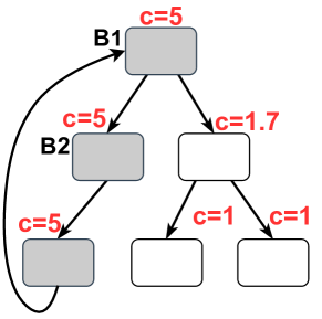
(a) Original CFG

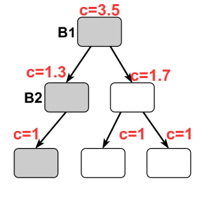
(b) Transformed CFG

Figure 4: Figure 4a shows that node B1 has the same centrality as node B2 as an artifact of the loop. However, B1 should have higher centrality than B2 because it can reach more edges. To resolve this, we remove loops from the CFG and Figure 4b shows the graph after this transformation.

Mitigating the effect of loops on centrality. Loops in a CFG can hurt the utility of a seed’s centrality score for seed selection. Figure 4a shows a level loop where node B1 and its child node B2 are assigned equal scores by a centrality analysis. However, nodes that initiate a loop should have more centrality than nodes in the loop body. In this case, the node that initiates the loop B1 should have higher centrality because it can reach more edges. To solve this problem, we convert the CFG to a directed acyclic graph by removing loops in the CFG. Such loops originate in program constructs such as while or for statements as well as connections between caller and callee nodes (i.e., caller to callee edge and callee to caller backedge can form a loop).

IV-B Influence Analysis

To compute a seed’s centrality, we could count the number of potentially reachable edges from a seed node in the edge horizon graph. However, this count assumes that all edges independent of distance are equally reachable and feasible which does not hold true for most real-world programs [61, 40]. Ideally, we want to count all feasible and reachable edges from a seed through mutations, but this is impractical to compute as it requires computing feasibility along all edges. Instead we use Katz centrality to approximate this count. Katz centrality provides three properties that make it a natural fit to approximate this count. First, it increases its approximation additively if more edges can be reached from a seed node independent of the order as described in Section II. Second, Katz centrality decreases its approximation if mutation frequency information suggests an edge is hard to reach or if edges are far away. Third, Katz centrality is efficient to compute with the power method as discussed in Section II.

Below, we explain how we set the mutation frequency information mechanism in Katz centrality and why Katz centrality multiplicatively decays contributions from further-away edges.

Using historical mutation data as a bias. We observe that $\mathbf{\beta}$ is a generic way of biasing a node’s centrality based on external information. We therefore use $\mathbf{\beta}$ to lower a node’s centrality if a node appears harder to reach by mutations. We set each element of $\mathbf{\beta}$ to range from 0 to 1, where values closer to 0 mean the node is harder to reach through mutations. To measure this hardness, we use historical mutation data. We initialize $\mathbf{\beta}=1$ if there are no mutations and iteratively refine it as a fuzzer generates mutations. We use the following equation for node i,

$$\beta_{i}=1-\frac{R_{i}}{T}$$ (8)

where $R_{i}$ measures the number of mutations that reach node i’s parents and $T$ measures the total number of mutations for all seeds.

Lastly, to set $\alpha$, which ranges from 0 to 1, from Equation 9, we observe that setting $\alpha=0$ means all nodes in the edge horizon graph will have the same centrality. This would not be useful for seed selection because we could not distinguish which seed node was more likely to discover new edge coverage with its centrality score. In contrast, setting $\alpha=1$ treats closer and further-away edges with equal contribution, which fails to reflect program behavior. In practice, we set $\alpha=0.5$ based on our experiments as described in Section VI.

Decaying contributions from longer paths. Katz centrality multiplicatively decays the contribution from further away edges when computing a node’s centrality . This decay corresponds to a well-known program behavior where further away edges are harder to reach by mutations [40]. We also verify this behavior with our own experiments in Appendix -B. To see how Katz centrality reduces the contribution from further-away edges toward a node’s centrality, consider Equation 9 which shows the 2nd iteration of the power method from Section II.

$$\mathbf{c}(2)=((\alpha)^{0}I+(\alpha)^{1}A+(\alpha)^{2}A^{2})\mathbf{\beta}$$ (9)

Notice how the parameter $\alpha$, which ranges between 0 and 1, multiplicatively decays the contribution from higher matrix powers. As discussed in Section II, higher matrix powers consider edges farther away. Thus, this equation shows Katz centrality reduces the contribution from further away edges with multiplicative decay.

IV-C Seed Scheduling

Algorithm 2 shows how to integrate K-Scheduler into a coverage-guided fuzzer. K-Scheduler first builds the edge horizon graph as shown in Algorithm 1 and computes the Katz centrality over it to measure each seed’s centrality. A fuzzer then uses these scores for seed scheduling which consists of selecting a seed and allocating a corresponding mutation budget. Because popular fuzzers such as AFL and LibFuzzer differ greatly in these two components, we abstract them out in lines 10 and 11 and specify how to integrate our generic technique into them in Section V. Finally, K-Scheduler re-computes the edge horizon graph and its Katz centrality when the fuzzer discovers new edge coverage or a fixed time has elapsed. Periodically updating centrality (i.e. via $\beta$) ensures that K-Scheduler provides useful guidance even when a fuzzer fails to find new edge coverage.

Algorithm 2 Fuzzer integration with K-Scheduler.

Input:	$G$ $\leftarrow$ Inter-procedural CFG
	$S$ $\leftarrow$ Seed corpus
	$P$ $\leftarrow$ Program

1:$stats=\{\}$ $\triangleright$ Store mutation statistics

2:$has\_new=False$ $\triangleright$ Indicate new edge coverage

3:$t=$ CreateTimer$(k)$ $\triangleright$ Build horizon graph every $k$ seconds

4:while fuzzer is running do

5:    if  $has\_new=True$ or $stats=\varnothing$ or $t.$timeout$()$ then

6:        $H=$ GetHorizonNodes$(G,S,P)$

7:        $Beta=$ ComputeBeta$(H,stats)$

8:        $G_{horizon}=$ GetHorizonGraph$(G,S,P)$

9:        $C_{katz}=$ KatzCentrality$(G_{horizon},Beta)$

10:        $t.$reset$()$ $\triangleright$ Reset timer $t$     

11:    $seed=$ ChooseSeed$(S,C_{katz})$

12:    $energy=$ ComputeEnergy$(seed,C_{katz})$

13:    $has\_new=$ Mutate$(seed,energy)$ $\triangleright$ Fuzz $seed$ with $energy$

14:    $stats.$update$()$

V Implementation

K-Scheduler consists of two components. First, to build the edge horizon graph, we construct the target program’s inter-procedural CFG. We initially compile the program with wllvm  [5] and use the LLVM’s (version 11.0.1) opt tool to extract each function’s intra-procedural CFG. In Python 3.7, we then merge each intra-procedural CFG together based on caller-callee relations to produce the inter-procedural CFG. We also implement all pieces from Algorithm 1 such as loop removal in Python. To classify CFG nodes as visited, we re-use a fuzzer’s edge coverage information to identify visited basic blocks. Second, to compute Katz centrality, we use the power method provided by networkit [4], a large-scale graph computing library.

We now describe how we integrate K-Scheduler into LibFuzzer [3] and AFL [62] to show our technique is generic and widely applicable. We run K-Scheduler as a standalone process that communicates with a fuzzer to set the fuzzer’s seed ranking based on centrality and identify the mapping between a seed node and its corresponding horizon nodes. We measure how much overhead K-Scheduler adds to the fuzzing process in Section VI.

Libfuzzer Integration. Libfuzzer [3] computes an energy for each seed in the form of a probability and flips a coin with bias corresponding to the seed’s energy to determine whether a seed should be selected for mutation. Higher energy probabilities indicate a seed will be chosen more frequently. To integrate into Libfuzzer, we follow the same integration as Entropic, a state-of-the-art seed scheduler for Libfuzzer, and set each seed’s energy to its Katz centrality score normalized by the total centrality scores for all seeds.

AFL Integration. Unlike Libfuzzer’s probabilistic seed selection, AFL generally selects every seed for mutation. A seed’s energy also determines its corresponding mutation budget. To integrate into AFL, we set each seed’s energy directly to its Katz centrality score.

VI Evaluation

Our evaluation aims to answer the following questions.

1. Comparison against seed schedulers: How does K-Scheduler compare against other seed scheduling strategies?

2. Bug Finding: Does K-Scheduler improve a fuzzer’s ability to find bugs?

3. Runtime Overhead: What is the performance overhead of K-Scheduler?

4. Impact of Design Choices: How do K-Scheduler’s various design choices contribute to its performance?

5. Non-evolutionary fuzzing settings: Does K-Scheduler show promise for seed scheduling in non-evolutionary fuzzing settings?

VI-A Experimental Setup

VI-A1 Baseline Seed Scheduling Strategies

We compare against popular seed scheduling strategies from industry and the academic community. These strategies are generally integrated into AFL or Libfuzzer. Directly comparing a seed scheduling strategy that uses AFL with another seed scheduling strategy that uses Libfuzzer can be misleading since the underlying fuzzers may cause the performance difference instead of the underlying seed scheduling strategy. Therefore, to be fair, we integrate K-Scheduler into both Libfuzzer and AFL separately and make comparisons about seed scheduling strategies when the underlying fuzzer is the same. Note this integration also demonstrates that K-Scheduler is generic and widely applicable.

For K-Scheduler’s comparison against Libfuzzer-based seed schedulers, we compare K-Scheduler against Entropic, a state-of-the-art seed scheduler in Libfuzzer [9]. To ensure a fair comparsion, we follow the same integration with Libfuzzer as Entropic. We also compare against Libfuzzer’s default seed scheduler as a baseline and refer to it as Default. We use Libfuzzer and Entropic from LLVM 11.0.1 in our comparison. For K-Scheduler’s comparison against AFL-based seed schedulers, we compare against strategies that prioritize seeds if they take paths rarely observed (RarePath), reach rarely observed edges (RareEdge) or discover new paths (NewPath). We also compare against a strategy that prioritizes seeds based on security-sensitive coverage (SecCov). To compare against RarePath, RareEdge, NewPath, and SecCov we use AFLFast [7], FairFuzz [32], EcoFuzz [60], and TortoiseFuzz [55] respectively. Since these fuzzers all modify AFL, we integrate K-Scheduler into AFL using their same modifications for a fair comparison. Moreover, we set each fuzzer to use the same mutation strategy to a enable a fair comparison. Hence, we disabled FairFuzz’s custom mutation strategy. We also compare against AFL’s default seed scheduling strategy as a baseline and refer to it as Default.

VI-A2 Benchmark Programs

In our seed scheduler comparison, we use the Google FuzzBench benchmark, a commonly used dataset to evaluate fuzzing performance on real-world programs. At the time of this writing, the benchmark consists of 40+ programs, so we decide to evaluate over a subset of them. We pick 12 diverse real-world programs from the benchmark that includes cryptographic and database programs as well as parsers as shown in Table III. We plan to evaluate against the entire benchmark in the future. We also use the default seed corpus and configuration provided by the benchmark to enable a fair comparison. Note that Google FuzzBench configures all AFL-based fuzzers to use havoc mode by default [1], since AFL havoc mode has been shown to significantly outperform AFL deterministic mode [58].

For our bug-finding experiments, we select 12 real-world parsing programs commonly used to evaluate fuzzer’s bug finding performance  [7, 32, 60]. The $12$ programs cover $8$ file formats: ELF, ZIP, PNG, JPEG, TIFF, TAR, TEXT and XML. The list of programs and their details can be found in Table VI. Since these programs do not come with a default seed corpus, we make a corpus with small valid files.

VI-A3 Environmental Setup

We run all our evaluations on $4$ 64-bit machines running Ubuntu 20.04 with Intel Xeon E5-2623 CPUs (96 cores in total). We follow standard operating procedure in fuzzing evaluations [7, 9, 32] and bound each fuzzer to 1 CPU core. Because our current implementation runs K-Scheduler in a separate process, we assign fuzzers using K-Scheduler 2 cores, one for the fuzzer and one for the K-Scheduler.

VI-B RQ1: Seed scheduling comparison

For K-Scheduler’s comparison against Libfuzzer-based seed schedulers, we follow the original evaluation of Entropic [9] and use the same two metrics for comparison: edge coverage and feature coverage. Edge coverage measures how many branches were reached along an input’s execution path, whereas feature coverage includes this information as well as branch hit count. For example, edge coverage would not distinguish coverage between two inputs that visit the same branch a different number of times, but feature coverage would distinguish them.

We run K-Scheduler, Default (i.e., Libfuzzer’s default seed scheduler), and Entropic on the 12 Google FuzzBench programs for 24 hours. We repeat each 24 hour run ten times for statistical power. In arithmetic mean over these 10 runs, Table  II and Table III summarize the edge and feature coverage results for 1 hour and 24 hours, respectively. Appendix Table XV and Table XVI show the corresponding result from applying the Mann Whitney U test between K-Scheduler and the tested seed schedulers in terms of edge and feature coverage. Within 1 hour, K-Scheduler improves upon next-best seed scheduling strategy Entropic by $20.11\%$ in median and $31.75\%$ in arithmetic mean over the 12 FuzzBench programs in feature coverage. For the 24 hour runs, K-Scheduler achieves $20.66\%$ in median and $25.89\%$ in arithmetic mean more feature coverage than Entropic. We attribute the increased improvement of K-Scheduler over Entropic within the first hour to K-Scheduler’s scheduling of promising seeds more frequently given a limited fuzzing budget (i.e., fuzzer only schedules a limited number of seeds). However, as the fuzzing budget increases to 24 hours, Entropic will eventually also schedule those promising seeds more frequently, which narrows the performance difference between K-Scheduler. Moreover, with a significance level of 0.05, our feature coverage over Entropic results are statistically significant for all programs for 24 hour runs and all programs except zlib for the 1 hour runs. Our results show that using the CFG structure for seed scheduling can improve fuzzing performance.

TABLE II: Arithmetic mean feature and edge coverage of Libfuzzer-based seed schedulers on 12 FuzzBench programs for 1 hour over 10 runs. We mark the highest number in bold.

Programs	K-Scheduler		Entropic		Default
	feature	edge	feature	edge	feature	edge
freetype	51,184	10,886	46,698	10,691	40,040	9,446
libxml2	39,240	7,661	24,167	6,128	25,914	6,296
lcms	2,886	1,497	1,707	1,004	1,392	874
harfbuzz	35,017	9,112	23,349	7,551	23,455	7,588
libjpeg	10,974	2,553	7,424	2,193	7,510	2,208
libpng	5,001	1,501	4,604	1,469	4,525	1,476
openssl	14,520	4,622	12,830	4,294	13,029	4,327
openthread	6,525	3,318	5,397	3,044	5,150	2,947
re2	31,292	6,275	28,877	6,147	29,941	6,207
sqlite	73,532	13,299	44,198	12,189	52,060	12,735
vorbis	9,106	2,136	7,632	2,010	5,710	1,823
zlib	2,711	790	2,572	784	2,408	782
Arithmetic mean coverage gain			31.75%	12.51%	37.37%	15.72%
Median coverage gain			20.11%	8.32%	34.54%	13.91%

TABLE III: Arithmetic mean feature and edge coverage of Libfuzzer-based seed schedulers on 12 FuzzBench programs for 24 hours over 10 runs. We mark the highest number in bold.

Programs	K-Scheduler		Entropic		Default
	feature	edge	feature	edge	feature	edge
freetype	71,717	13,754	75,370	14,120	67,510	12,870
libxml2	54,081	9,869	36,958	7,038	39,247	7,310
lcms	6,345	2,541	4,425	2,082	3,413	1,784
harfbuzz	48,105	10,358	32,799	8,808	33,499	8,912
libjpeg	15,861	3,033	11,755	2,646	11,220	2,574
libpng	5,312	1,535	5,002	1,501	4,992	1,501
openssl	16,644	4,971	15,137	4,731	15,173	4,738
openthread	11,405	4,965	6,435	3,276	6,123	3,196
re2	33,797	6,482	32,401	6,347	32,725	6,367
sqlite	92,493	15,540	75,723	14,351	83,228	14,710
vorbis	10,417	2,247	9,906	2,208	8,873	2,115
zlib	3,215	801	2,698	790	2,510	787
Arithmetic mean coverage gain			25.89%	13.69%	31.43%	16.34%
Median coverage gain			20.66%	6.68%	22.75%	6.54%

For K-Scheduler’s comparison against AFL-based seed schedulers, we only use edge coverage as a metric for comparison because AFL does not report feature coverage. We run K-Scheduler, Default (i.e., AFL’s default seed scheduler), RarePath, RareEdge, NewPath, and SecurityCov on the same 12 Google FuzzBench programs for 24 hours, repeated ten times. In arithmetic mean over these 10 runs, Table  IV and Table  V summarize the edge coverage results for 1 hour and 24 hours respectively. Appendix Table XVII and Table XVIII show the Mann-Whitney U test results. Similar to the comparison against Libfuzzer-based seed schedulers, we observe a higher improvement of K-Scheduler over the other seed scheduling strategies within the first hour. K-Scheduler outperforms the next best seed scheduling strategy (RarePath) by 7.95% in arithmetic mean and 3.62% in median over the 12 FuzzBench programs. For the 24 hour runs, K-Scheduler achieves 4.21% in arithmetic mean and 1.91% in median more coverage than RarePath. We note that the improvement of K-Scheduler against AFL-based seed schedulers is not as significant as K-Scheduler’s comparison against Libfuzzer-based seed schedulers. We believe K-Scheduler’s diminished performance difference occurs because the underlying fuzzer, AFL, iterates over the seed queue multiple times during the 24 hours fuzzing campaign and therefore will schedule nearly all seeds frequently, reducing the effect of seed selection.

TABLE IV: Arithmetic mean edge coverage of AFL-based seed schedulers on 12 FuzzBench programs for 1 hour over 10 runs.

	K-Sched	Default	RarePath	RareEdge	NewPath	SecCov
Fuzzer	AFL	AFL	AflFast	FairFuzz	EcoFuzz	TortoiseFuzz
freetype	12,077	11,001	10,707	11,319	8,925	10,532
libxml2	8,120	5,793	5,836	7,247	5,841	5,476
lcms	1,882	1,989	1,540	1,343	1,117	1,327
harfbuzz	9,169	8,864	9,022	8,767	7,629	8,773
libjpeg	2,391	2,354	2,374	2,140	1,739	2,073
libpng	1,470	1,488	1,460	1,430	1,428	1,456
openssl	4,560	4,485	4,399	4,381	4,252	4,336
openthread	5,245	5,063	5,064	5,047	5,047	5,012
re2	5,792	5,612	5,533	5,335	5,484	5,252
sqlite	9,865	10,038	9,890	10,065	9,722	9,627
vorbis	2,048	2,006	1,946	1,933	1,761	1,914
zlib	761	758	752	746	745	752
Arithmetic mean gain		4.80%	7.95%	8.39%	20.01%	13.03%
Median gain		1.87%	3.62%	5.27%	11.77%	6.07%

TABLE V: Arithmetic mean edge coverage of AFL-based seed schedulers on 12 FuzzBench programs for 24 hours over 10 runs.

	K-Sched	Default	RarePath	RareEdge	NewPath	SecCov
Fuzzer	AFL	AFL	AflFast	FairFuzz	EcoFuzz	TortoiseFuzz
freetype	14,188	13,508	13,646	13,486	11,965	13,206
libxml2	10,936	9,295	8,546	10,241	8,964	9,147
lcms	2,325	2,247	2,160	2,190	1,892	2,162
harfbuzz	10,061	9,980	10,019	9,804	9,946	9,882
libjpeg	2,678	2,513	2,601	2,497	2,309	2,413
libpng	1,536	1,536	1,535	1,524	1,528	1,528
openssl	4,863	4,805	4,761	4,788	4,732	4,685
openthread	5,766	5,704	5,646	5,666	5,527	5,636
re2	5,887	5,875	5,790	5,536	5,774	5,758
sqlite	12,081	12,360	12,019	10,648	12,199	11,810
vorbis	2,215	2,195	2,202	2,100	2,171	2,184
zlib	780	780	775	778	777	769
Arithmetic mean gain		2.89%	4.21%	4.81%	7.63%	5.11%
Median gain		1.00%	1.91%	5.34%	2.38%	2.30%

The coverage plots over time also highlight the promise of K-Scheduler. Figure 5 and 6 show that K-Scheduler generally maintains its performance advantage during the lifetime of the fuzzing campaign. The consistency of K-Scheduler’s gain across many different seed schedulers show the promise of scheduling seeds based on CFG information. Moreover, it suggests K-Scheduler can be helpful independent of a fuzzer as we later explore.

Result 1: K-Scheduler increases feature coverage by 25.89% compared to Entropic and edge coverage by 4.21% compared to the next-best AFL-based seed scheduler (RarePath), in arithmetic mean on 12 Google FuzzBench programs.

VI-C RQ2: Bug Finding

In order to detect memory corruption bugs that do not necessarily lead to a crash, we compile program binaries with Address and Undefined Behavior Sanitizers. We then ran K-Scheduler, Default (i.e., AFL’s default seed scheduler), RarePath, RareEdge, and NewPath on 12 real-world parsing programs for 24 hours, a total of 10 times. We could not run the Libfuzzer-based seed schedulers because the 12 parsing programs are not equipped with a Libfuzzer-compatible fuzzing harness (i.e., LLVMFuzzerTestOneInput is undefined).

In our 24 hour runs, we found real-world bugs in binutils. Table VII shows the bug count for each seed scheduling strategy in terms of integer overflow, out of memory and memory leak bugs, in arithmetic mean over the 10 runs. We count bugs with the following procedure based on prior work [6, 15, 48]. We first use AFL-CMin to reduce the number of crashing inputs. We then further deduplicate the crashing inputs by filtering them by unique stack traces. We lastly triage the remaining crashing inputs by manually reviewing their stack traces and corresponding source code. Our results show that K-Scheduler finds 3 more bugs than the next best seed scheduling strategy SecCov (i.e., TortoiseFuzz), which optimizes for bug-finding.

TABLE VI: Tested Programs in Bug Finding Experiments.

Subjects	Version	Format	# lines
xmllint	libxml2-2.9.7	XML	72,630
miniunz	zlib-1.2.11	ZIP	1,895
readpng	libpng-1.6.37	PNG	3,205
djpeg	libjpeg-9d	JPEG	9,204
size	binutils-2.36.1	ELF	51,203
readelf -a	binutils-2.36.1	ELF	29,954
nm -C	binutils-2.36.1	ELF	52,763
objdump -D	binutils-2.36.1	ELF	78,610
strip	binutils-2.36.1	ELF	59,680
tiff2pdf	tiff-4.3.0	TIFF	20,387
bsdtar -xf	libarchive-3.5.1	TAR	45,031
infotocap	ncurses-6.2	TEXT	23,145

TABLE VII: Overview of bugs discovered in our AFL-based seed scheduling experiments categorized by type.

	K-Sched	Default	RarePath	RareEdge	NewPath	SecCov
Fuzzer	AFL	AFL	AflFast	FairFuzz	EcoFuzz	Tortoise$\dagger$
out-of-memory	21	14	19	17	18	21
memory leak	24	20	21	19	20	22
integer overflow	3	2	3	3	2	2
Total	48	36	43	39	40	45

$\dagger$ Tortoise denotes TortoiseFuzz.

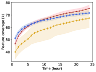
(a) freetype

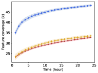
(b) harfbuzz

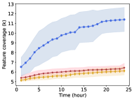
(c) openthread

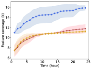
(d) libjpeg

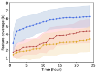
(e) lcms

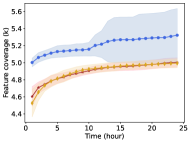
(f) libpng

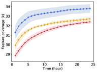
(g) re2

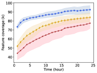
(h) sqlite

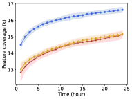
(i) openssl

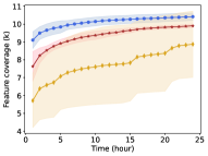
(j) vorbis

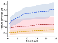
(k) zlib

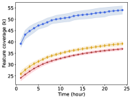
(l) libxml2

Figure 5: The arithemic mean feature coverage of Libfuzzer-based seed schedulers running for 24 hours and one standard deviation error bars over 10 runs. Default refers to the default seed scheduler in Libfuzzer.

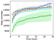
(a) freetype

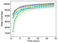
(b) harfbuzz

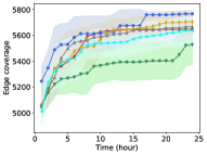
(c) openthread

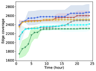
(d) libjpeg

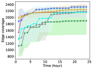
(e) lcms

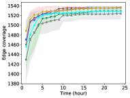
(f) libpng

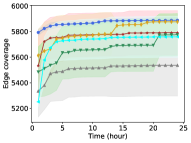
(g) re2

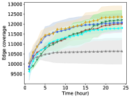
(h) sqlite

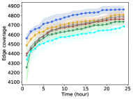
(i) openssl

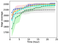
(j) vorbis

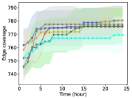
(k) zlib

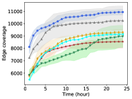
(l) libxml2

Figure 6: The arithmetic mean edge coverage of of AFL-based seed schedulers running for 24 hours and one standard deviation error bars over 10 runs. Default refers to the default seed scheduler in AFL.

Result 2: K-Scheduler discovers 3 more bugs than the next best seed-scheduling strategy (SecCov).

VI-D RQ3: Runtime Overhead

In this experiment, we measure the overhead that K-Scheduler adds to a fuzzer. The runtime overhead can be classified into two components: a fuzzer maintenance (i.e., record hit count of edges and compute seeds’ energy) and a fuzzer invoking K-Scheduler (i.e., construct edge horizon graph and perform Katz centrality analysis) for seed scheduling. To measure these overheads, we run our modified versions (see Section V) of AFL and Libfuzzer against all 12 FuzzBench programs for 24 hours, recording the total time they spend in maintenance and separately the total time spent in computing Katz centrality over the edge horizon graph in the standalone process. We repeat this experiment 10 times to minimize variance. Table VIII summarizes the runtime overhead added to AFL’s and LibFuzzer fuzzing processes in terms of fuzzer maintenance and graph centrality analysis.

The overhead of fuzzer maintenance is $0.28\%$ for AFL and $1.74\%$ for Libfuzzer, in arithmetic mean over the 12 FuzzBench programs. The graph analysis overhead is minimal, adding $0.15\%$ in arithmetic mean over the 12 FuzzBench programs. We believe these small graph analysis overheads exist because Katz centrality can be efficiently computed with the power method (Section II) and the edge horizon graph is cached and updated instead of being constructed from scratch each time. For clarity, we did not report graph analysis overheads for AFL and Libfuzzer separately because they use the same standalone process, so the overheads were nearly indistinguishable. Moreover, the difference in overheads per-program is explained by the variance in the target program’s CFG size (i.e., number of nodes).

Result 3: K-Scheduler adds at most $1\%$ overhead from graph analysis and at most $2\%$ overhead for fuzzer maintenance.

VI-E RQ4: Impact of Design Choices

TABLE VIII: Runtime overhead from K-Scheduler in Libfuzzer and AFL-based seed scheduling.

Programs	Nodes #	Graph Analysis	Fuzzer Maintenance
			LibFuzzer	AFL
freetype	38,352	0.20%	1.71%	0.23%
libxml2	96,732	0.22%	2.53%	0.39%
lcms	13,081	0.06%	0.92%	0.08%
harfbuzz	21,066	0.11%	2.25%	0.17%
libjpeg	16,508	0.04%	0.79%	0.06%
libpng	7,215	0.02%	0.53%	0.03%
openssl	57,729	0.25%	2.43%	0.67%
openthread	27,263	0.09%	1.48%	0.24%
re2	12,020	0.03%	1.39%	0.26%
sqlite	70,703	0.75%	3.12%	0.41%
vorbis	9,494	0.04%	0.80%	0.55%
zlib	1,882	0.02%	2.96%	0.29%
Arithmetic mean	31,004	0.15%	1.74%	0.28%
Median	18,787	0.08%	1.60%	0.25%

We conduct experiments to measure the performance effect of five design choices: (i) centrality measure, (ii) $\mathbf{\beta}$ parameterization, (iii) visited node deletion, (iv) loop removal, and (v) $\alpha$ parameterization. For each design choice experiment, we run K-Scheduler with Libfuzzer on the 12 Google FuzzBench programs for 1 hour, repeated 10 times, and compare their feature coverage. We run for 1 hour because the first hour of a fuzzing run often discovers more coverage than later hours and hence our results better measure the effect of the design choices. We also choose feature coverage because it provides more fine-grained information about a fuzzer’s behavior than edge coverage. We describe each design choice experiment in more detail below.

VI-E1 Centrality measure

We measure the effect of the centrality measure on seed scheduling in this experiment by varying the centrality measure used in K-Scheduler. We compare Eigenvector, Degree, Katz and PageRank centrality measures. Table IX shows the feature coverage results. Enabling Katz centrality improves the feature coverage by $16.54\%$, $23.69\%$, and $19.17\%$ in arithmetic mean over the 12 FuzzBench programs, relative to Pagerank, Eigenvector, and Degree centrality, respectively. These results experimentally justify our claim from Section II that Katz centrality is most desirable for seed scheduling. However, these results also show that for some programs, other forms of centrality are a better fit such as the superior performance of Pagerank on re2 and Degree on vorbis.

TABLE IX: Arithmetic mean feature coverage of K-Scheduler with different centrality metrics.

Programs	Katz	Pagerank	Eigenvector	Degree
freetype	51,184	44,394	40,723	38,332
libxml2	39,240	29,575	28,473	28,014
lcms	2,886	2,071	1,557	2,054
harfbuzz	35,017	28,563	26,253	27,485
libjpeg	10,974	9,250	10,454	8,713
libpng	5,001	4,804	4,505	4,923
openssl	14,520	13,035	13,385	13,555
openthread	6,525	5,201	5,380	5,298
re2	31,292	32,309	29,648	29,595
sqlite	73,532	68,328	65,538	63,997
vorbis	9,106	8,129	7,470	9,363
zlib	2,711	2,410	2,323	2,404
Arithmetic mean coverage gain		16.54%	23.69%	19.17%
Median coverage gain		13.89%	18.99%	19.03%

VI-E2 $\mathbf{\beta}$ parameterization

In Section IV, we describe how we set $\mathbf{\beta}$ based on historical mutation data. In this comparison, we see the effect of this technique by comparing K-Scheduler with uniform $\mathbf{\beta}$ against K-Scheduler with non-uniform $\mathbf{\beta}$. Table X shows the feature coverage results. The non-uniform $\mathbf{\beta}$ technique increases feature coverage by $24.19\%$ in arithmetic mean over the 12 FuzzBench programs. These results show the utility of biasing $\mathbf{\beta}$.

TABLE X: Arithmetic mean feature coverage from analyzing the effect of non-uniform $\mathbf{\beta}$.

Programs	Non-uniform $\mathbf{\beta}$	Uniform $\mathbf{\beta}$
freetype	51,184	40,396
libxml2	39,240	31,733
lcms	2,886	1,506
harfbuzz	35,017	29,380
libjpeg	10,974	8,834
libpng	5,001	4,761
openssl	14,520	12,542
openthread	6,525	5,271
re2	31,292	28,263
sqlite	73,532	64,893
vorbis	9,106	7,679
zlib	2,711	2,305
Arithmetic mean coverage gain		24.19%
Median coverage gain		18.88%

TABLE XI: Arithmetic mean feature coverage from analyzing the effect of $\alpha$.

Programs	0.5	0.25	0.75	1
freetype	51,184	38,369	41,777	40,723
libxml2	39,240	28,644	29,992	28,473
lcms	2,886	1,313	1,552	1,557
harfbuzz	35,017	27,250	28,276	26,253
libjpeg	10,974	9,542	10,336	10,454
libpng	5,001	4,913	4,929	4,505
openssl	14,520	13,420	13,302	13,385
openthread	6,525	6,216	5,597	5,380
re2	31,292	29,590	31,885	29,648
sqlite	73,532	64,175	68,550	65,538
vorbis	9,106	8,092	8,066	7,470
zlib	2,711	2,378	2,282	2,323
Arithmetic mean coverage gain		24.53%	19.47%	23.69%
Median coverage gain		14.29%	14.74%	18.99%

TABLE XII: Arithmetic mean feature coverage from analyzing the effect of loop removal.

Programs	loop removal	no loop removal
freetype	51,184	38,646
libxml2	39,240	28,737
lcms	2,886	1,455
harfbuzz	35,017	28,849
libjpeg	10,974	10,142
libpng	5,001	4,846
openssl	14,520	13,300
openthread	6,525	5,430
re2	31,292	31,609
sqlite	73,532	64,560
vorbis	9,106	9,350
zlib	2,711	2,247
Arithmetic mean coverage gain		21.70%
Median coverage gain		17.03%

VI-E3 Visited node deletion

In Section IV, we describe why we remove visited nodes from the edge horizon graph. In this comparison, we experimentally justify this choice. We compare K-Scheduler with visited node deletions from the edge horizon graph against K-Scheduler with no deletions from the edge horizon graph. Table XIII shows the feature coverage results. The deleted edge horizon graph improves feature coverage by $24.13\%$ in arithmetic mean over the 12 FuzzBench programs. Therefore, this result justifies our deletion of visited nodes.

TABLE XIII: Arithmetic mean feature coverage from analyzing the effect of deleting visited nodes.

Programs	Original	Deleted
freetype	51,184	39,892
libxml2	39,240	28,973
lcms	2,886	1,493
harfbuzz	35,017	24,667
libjpeg	10,974	9,715
libpng	5,001	4,827
openssl	14,520	13,121
openthread	6,525	5,712
re2	31,292	29,408
sqlite	73,532	61,609
vorbis	9,106	8,020
zlib	2,711	2,470
Arithmetic mean coverage gain		24.13%
Median coverage gain		13.89%

VI-E4 Loop Removal

In Section IV, we introduce our loop removal transform as a technique to mitigate the effects of loops on computing centrality. In this experiment, we measure this effect by comparing K-Scheduler with and without the loop removal transform. Table XII shows that the loop removal transform improves edge coverage by $21.70\%$ in arithmetic mean over the 12 FuzzBench programs, justifying our loop removal transform.

VI-E5 $\alpha$ parameterization

In this design choice experiment, we study how the choice of $\alpha$ affects the K-Scheduler’s performance. Table XI summarizes our findings. As described in Section IV, $\alpha=1$ treats far and close paths with equal contribution to centrality and its experimental results are worse compared to distinguishing them, showing the utility of the multipicative decay effect. We note that $\alpha=1$ is equivalent to Eigenvector centrality as seen by comparing the relevant column from Table IX. Given $\alpha=0.5$ performs best in arithmetic mean over the 12 FuzzBench programs, we pick it in our current implementation.

Result 4: Our results empirically support K-Scheduler’s design choices.

VI-F RQ5: Utility for non-evolutionary input generation

In this experiment, we show the promise of K-Scheduler in non-fuzzing settings, we integrate K-Scheduler into concolic execution seed scheduling. Concolic execution is known to incur high overhead [61, 42] during path constraint collection and solving. Hence, in concolic execution, scheduling promising seeds is crucial to its performance [16, 63]. To perform this experiment, we use the concolic executor from QSYM’s latest version [61]. QSYM, a hybrid fuzzer, consists of three components, a concolic executor, a fuzzer, and a coordinator that schedules seeds for the concolic executor. Since our goal is to show the utility of K-Scheduler for concolic execution seed scheduling, we disabled QSYM’s fuzzer and only modified its coordinator’s seed scheduling algorithm to use K-Scheduler. We did not modify QSYM’s concolic executor logic. We evaluate on the $3$ programs (size, libarchive and tcpdump). Note we did not run on SymCC because SymCC and QSYM have the same concolic execution scheduler [42], so comparing against one is sufficient. We run K-Scheduler against the default seed scheduler in QSYM on the $3$ real world programs for $24$ hours and compare the total edge coverage. In arithmetic mean over the 10 runs, Table  XIV shows that K-Scheduler improves edge coverage by $35.76\%$, in arithmetic mean over the 3 programs. Hence, this shows the potential promise K-Scheduler for seed scheduling in non-evolutionary fuzzing settings.

TABLE XIV: Edge coverage of concolic-execution-based seed scheduling on 3 real-world programs for 24 hours over 5 runs.

Scheduling	K-Scheduler	Default
libarchive	3,886	3,230
size	3,068	2,602
tcpdump	3,552	2,101
Arithmetic mean coverage gain		35.76%
Median coverage gain		20.31%

However, we note that our results are preliminary and are inconclusive. We leave a detailed evaluation to future work.

Result 5: K-Scheduler increases edge coverage by $35.76\%$, in arithmetic mean over 3 programs, compared to QSYM’s default seed scheduling strategy.

VII Related Work

VII-A Graph Centrality

Centrality is a commonly used measure in graph analysis. Researchers have proposed various centrality metrics including degree centrality [47], semi-local centrality [14], closeness centrality [45], betweenness centrality [21], eigenvector centrality [51], Katz centrality [30], and PageRank [10]. These centrality measures has been applied to various fields such as social network analysis [27, 11], biology [31], finance [44] and geography [19]. To the best of our knowledge, we are the first to use centrality for seed selection in fuzzing.

VII-B Seed Scheduling

While prior work has proposed a wide range of techniques to improve fuzzing such as symbolic execution [12, 24, 25, 49, 61, 40, 17, 50], dynamic taint analysis [54, 15, 23, 22, 43] and machine learning [26, 48, 65], in this paper we focus on improving the seed scheduling component in a fuzzer. We describe prior work that has focused on improving fuzzing through seed scheduling. Seed scheduling consists of two main components: input prioritization [55, 52, 53] and the input’s corresponding mutation budget (i.e., power schedule) [9, 7]. Prior seed scheduling work has prioritized seeds based on edge or path coverage [32, 7, 9, 60] as well as more security-sensitive metrics such as execution time [41, 33], exploitability [57], memory accesses [18, 56, 55], or a combination of them [52, 53] Another line of work prioritizes seeds based on call graphs [34]. In contrast, we prioritize seeds based on the entire inter-procedural CFG. While AFLGo [8] also uses the entire inter-procedural CFG, it computes the distance over the CFG for directed fuzzing and assigning a seed’s mutation budget. In contrast, we approximate the count of reachable and feasible edges from a seed and use it for coverage-guided fuzzing. SAVIOR [17] also approximates this count but uses it for bug-driven hybrid testing. Its approximation assumes all edges are equally likely to be reachable and feasible, independent of their distance from a seed’s execution path, which does not hold true for many real-world programs as we showed in Section VI. In contrast, we use the multiplicative decay property of Katz centrality to reflect this behavior in real-world programs and better approximate this count. Moreover, SAVIOR [17]’s approximation is equivalent to setting $\alpha=1$ (i.e, no multiplicative decay) and our design choice experiments show this approximation performs worse than K-Scheduler’s default settings. Nonetheless, both K-Scheduler and SAVIOR utilize the mutation history information to improve their approximation.

Seed scheduling has also been a topic in other program testing techniques aside from fuzzing such as concolic execution [16, 63]. Our preliminary experiments suggest that K-Scheduler can improve seed scheduling for concolic execution.

VIII conclusion

In this paper, we introduce a new approach to seed scheduling based on centrality analysis of seeds on the CFG. Centrality measures have several desirable properties that make them a natural fit for the seed scheduling problem. We implement our approach in K-Scheduler and show its effectiveness in seed scheduling: increasing feature coverage by 25.89% compared to Entropic and edge coverage by 4.21% compared to the next-best AFL-based seed scheduler, in arithmetic mean on 12 Google FuzzBench programs.

-A Mann-Whitney U Test Results

TABLE XV: Mann-Whitney U test results over the feature and edge coverage of Libfuzzer-based seed schedulers on 12 FuzzBench programs for 1 hour over 10 runs (corresponding to Table II).

Programs	Entropic		Default
	feature	edge	feature	edge
freetype	4.40E-4	1.62E-2	7.69E-4	1.71E-3
libxml2	1.83E-4	1.82E-4	1.83E-4	1.83E-4
lcms	3.61E-3	1.31E-3	1.83E-4	1.83E-4
harfbuzz	1.82E-4	1.83E-4	1.83E-4	1.82E-4
libjpeg	1.83E-4	1.82E-4	1.83E-4	1.82E-4
libpng	1.82E-4	1.68E-4	1.81E-4	1.67E-4
openssl	1.83E-4	1.82E-4	1.83E-4	1.82E-4
openthread	1.83E-4	2.19E-3	1.83E-4	1.83E-4
re2	2.46E-4	3.28E-4	1.71E-3	2.47E-3
sqlite	1.83E-4	1.83E-4	1.83E-4	1.73E-2
vorbis	4.40E-4	7.69E-4	2.46E-4	2.46E-4
zlib	8.90E-2	6.72E-2	1.31E-3	6.13E-2

TABLE XVI: Mann-Whitney U test results over the fuzzer and edge coverage of Libfuzzer-based seed schedulers on 12 FuzzBench programs for 24 hours over 10 runs (corresponding to Table III).

Programs	Entropic		Default
	feature	edge	feature	edge
freetype	1.70E-3	7.56E-2	2.12E-1	3.12E-2
libxml2	1.83E-4	1.83E-4	1.83E-4	1.83E-4
lcms	3.61E-3	9.11E-3	2.20E-3	3.61E-3
harfbuzz	1.83E-4	1.82E-4	1.83E-4	1.82E-4
libjpeg	1.83E-4	2.45E-4	1.83E-4	1.82E-4
libpng	1.31E-3	2.89E-4	7.58E-4	2.74E-4
openssl	1.82E-4	1.82E-4	1.83E-4	1.80E-4
openthread	1.83E-4	1.83E-4	1.83E-4	1.83E-4
re2	3.30E-4	3.17E-3	7.65E-4	3.60E-3
sqlite	1.83E-4	1.01E-3	1.31E-3	3.76E-2
vorbis	1.83E-4	2.40E-4	1.83E-4	4.33E-4
zlib	2.19E-3	5.65E-3	1.82E-4	3.84E-3

TABLE XVII: Mann-Whitney U test results over the fuzzer and edge coverage of AFL-based seed schedulers on 12 FuzzBench programs for 1 hour over 10 runs (corresponding to Table IV).

	Default	RarePath	RareEdge	NewPath	SecCov
Fuzzer	AFL	AflFast	FairFuzz	EcoFuzz	TortoiseFuzz
freetype	2.16E-3	2.16E-3	2.16E-3	2.16E-3	2.16E-3
libxml2	2.16E-3	2.16E-3	2.16E-3	2.16E-3	2.16E-3
lcms	8.18E-2	1.99E-2	1.52E-3	4.33E-4	9.31E-3
harfbuzz	2.16E-3	2.47E-2	2.60E-2	2.16E-3	8.13E-3
libjpeg	5.75E-2	6.87E-2	6.46E-3	4.99E-4	2.01E-3
libpng	8.86E-2	8.85E-2	1.71E-2	1.71E-2	6.10E-2
openssl	1.14E-2	2.86E-3	9.52E-4	9.52E-4	9.52E-4
openthread	2.00E-2	1.14E-2	1.14E-2	3.81E-3	6.63E-3
re2	8.67E-3	9.31E-2	2.16E-3	2.16E-3	2.16E-3
sqlite	5.89E-2	1.01E-1	3.10E-2	3.10E-2	3.94E-2
vorbis	2.45E-2	8.14E-3	6.63E-3	9.52E-4	1.14E-2
zlib	8.82E-2	4.65E-2	1.99E-2	2.58E-3	3.34E-2

TABLE XVIII: Mann-Whitney U test results over the fuzzer and edge coverage of AFL-based seed schedulers on 12 FuzzBench programs for 24 hours over 10 runs (corresponding to Table V).

	Default	RarePath	RareEdge	NewPath	SecCov
Fuzzer	AFL	AflFast	FairFuzz	EcoFuzz	TortoiseFuzz
freetype	5.89E-2	8.18E-2	4.85E-2	2.16E-4	6.49E-3
libxml2	2.16E-3	2.16E-3	1.80E-2	2.16E-3	2.16E-3
lcms	3.10E-2	2.41E-2	6.49E-3	2.16E-4	2.41E-2
harfbuzz	1.32E-2	5.89E-2	2.16E-4	6.49E-3	1.52E-3
libjpeg	3.91E-2	8.20E-2	6.51E-3	2.16E-4	2.01E-3
libpng	7.70E-2	1.12E-1	5.35E-3	2.39E-3	1.30E-2
openssl	3.43E-2	1.14E-2	1.14E-2	9.52E-4	9.52E-4
openthread	4.86E-2	2.87E-3	2.57E-2	9.52E-4	1.14E-2
re2	3.94E-2	1.09E-2	2.60E-3	1.29E-3	8.65E-4
sqlite	6.99E-2	8.18E-2	1.51E-3	9.37E-2	3.94E-2
vorbis	2.01E-2	2.85E-3	1.87E-3	1.65E-2	3.92E-2
zlib	9.35E-2	2.40E-2	1.34E-2	5.79E-2	1.93E-2

-B Further-away Edges Are Harder to Reach by Mutations

We run an experiment verifying our observation that further away edges in programs are harder to reach by mutations. In Section IV, we claimed that further away edges are harder to reach by mutations. This program property justified Katz centrality, which decays the contribution from further out edges. To validate this claim, we measure the likelihood that a seed mutation will reach further-away edges on 3 real-world programs. For each program, we choose $10$ seeds and mutate each seed 10,000 times. We repeat this process 10 times to minimize variance. Figure 7 shows the result, where n-hop indicates distance n from the original seed’s execution path. This experimentally shows that fewer mutations will reach farther away edges and hence further-away edges are harder to reach by mutations.

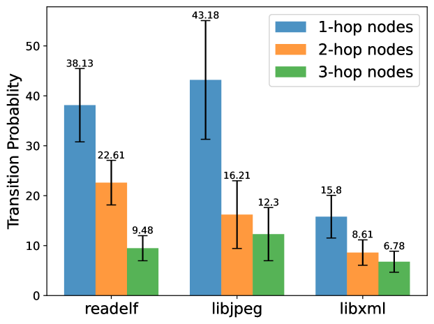
Figure 7: The transition probability on 3 real-world programs using 10 seeds with 10,000 mutations per seed. The 1-hop transition probability indicates the normalized amount of mutations that reached an edge of distance 1 from the current execution path, and similarly for 2-hop and 3-hop.

-C K-Scheduler’s Approximation Accuracy

In this section, we run an experiment to show the accuracy of Katz centrality in approximating the count of reachable and feasible edges. In Section IV, we claimed that an ideal seed scheduling strategy would prioritize seeds based on the count of all reachable and feasible edges from a seed by mutations. To better support this claim, we measure how much agreement exists between K-Scheduler’s centrality-based ranking with this ideal seed scheduler’s ranking. We simulate the ideal seed scheduler’s ranking by computing each CFG node’s count of reachable and feasible edges based on graph traversal and covered edges (i.e., feasible) from 24 hour runs of Libfuzzer with K-Scheduler over all 12 FuzzBench programs, repeated 10 times. We then use the Kendall tau independence test to measure the agreement between two rankings with a value between [-1, 1] and report if the measured agreement is statistically significant. We note this Kendall tau independence test and its p-values are entirely separate from the Mann Whitney U test and its p-values from our edge coverage experiments.

Table XIX shows the results from the Kendall tau independence test. The absolute values of the correlation are expectedly small given the large size of the ranking lists (on the order of thousands). K-Scheduler’s centrality-based rankings and the ideal strategy’s ranking strongly agree on 10 of the 12 programs (i.e., positive correlation values). On 8 of these 10 programs, this agreement is statistically significant with a significance level of $0.05$. This agreement suggests that K-Scheduler’s increased performance in our edge coverage experiments derives from approximating this ideal seed scheduling strategy and that improved approximations would lead to better seed scheduling strategies.

TABLE XIX: Using the Kendall tau independence test to measure the agreement between K-Scheduler’s per node rankings with the ideal seed scheduling ranking (i.e., the count of all reachable and feasible edges from a node). The correlation score ranges between $[-1,1]$, with higher values indicating stronger agreement. Given the the absolute value of the correlation is small due to the large size of the ranking list (i.e., thousands of nodes), we also report the p-value and statistical significance under a 0.05 significance level.

Programs	Correlation	p-value	Statistical
			Significance
freetype	0.01	8.9E-1	$\times$
libxml2	0.03	1.33E-58	✓
lcms	0.06	4.10E-24	✓
harfbuzz	0.09	4.58E-80	✓
libjpeg	-0.03	4.72E-9	✓
libpng	0.05	2.24E-9	✓
openssl	0.01	3.4E-1	$\times$
openthread	-0.01	1.12E-5	✓
re2	0.01	2.01E-2	✓
sqlite	0.06	4.24E-107	✓
vorbis	0.04	3.47E-6	✓
zlib	0.07	1.92E-5	✓

-D Limitations

K-Scheduler does not currently handle indirect function calls. We plan to handle them with static analysis techniques (e.g., Andersen’s points-to analysis) similar to prior work [17]. Such a static analysis may produce imprecise CFGs which can affect the utility of a seed’s centrality score for seed selection. However, K-Scheduler can mitigate the effects of imprecise CFGs on centrality by reducing the contributions from further away nodes (i.e. nodes in callee functions). Therefore, we believe K-Scheduler will still provide useful guidance despite the imprecision of the CFG. We also envision using $\beta$ for specific CFG nodes (i.e., nodes with indirect function calls) to further mitigate the effects of imprecise CFGs on centrality. We leave this to future work.

References

- Fuz [2021] FuzzBench guidelines about setting havoc mode for AFL evaluation. https://github.com/google/fuzzbench/blob/master/fuzzers/afl/fuzzer.py#L113, 2021.
- hon [2021] Honggfuzz - A security oriented, feedback-driven, evolutionary, easy-to-use fuzzer with interesting analysis options. https://github.com/google/honggfuzz, 2021.
- lib [2021] libFuzzer – a library for coverage-guided fuzz testing. https://llvm.org/docs/LibFuzzer.html, 2021.
- net [2021] Networkit: Large-scale Network Analysis. https://networkit.github.io/, 2021.
- wll [2021] Whole Program LLVM. https://github.com/travitch/whole-program-llvm, 2021.
- Aschermann et al. [2019] Cornelius Aschermann, Sergej Schumilo, Tim Blazytko, Robert Gawlik, and Thorsten Holz. Redqueen: Fuzzing with input-to-state correspondence. In Symposium on Network and Distributed System Security (NDSS), 2019.
- Böhme et al. [2016] Marcel Böhme, Van-Thuan Pham, and Abhik Roychoudhury. Coverage-based greybox fuzzing as markov chain. In Proceedings of the ACM SIGSAC Conference on Computer and Communications Security (CCS), pages 1032–1043. ACM, 2016.
- Böhme et al. [2017] Marcel Böhme, Van-Thuan Pham, Manh-Dung Nguyen, and Abhik Roychoudhury. Directed greybox fuzzing. CCS ’17, New York, NY, USA, 2017. Association for Computing Machinery.
- Böhme et al. [2020] Marcel Böhme, Valentin J. M. Manès, and Sang Kil Cha. Boosting fuzzer efficiency: An information theoretic perspective. In Proceedings of the 28th ACM Joint Meeting on European Software Engineering Conference and Symposium on the Foundations of Software Engineering, ESEC/FSE 2020, New York, NY, USA, 2020. Association for Computing Machinery.
- Brin and Page [1998] S. Brin and L. Page. The anatomy of a large-scale hypertextual web search engine. In Seventh International World-Wide Web Conference (WWW 1998), 1998.
- Brown and Hayes [2008] Duncan Brown and Nick Hayes. Influencer marketing. Routledge, 2008.
- Cadar et al. [2008] Cristian Cadar, Daniel Dunbar, and Dawson Engler. Klee: Unassisted and automatic generation of high-coverage tests for complex systems programs. In Proceedings of the 8th USENIX Conference on Operating Systems Design and Implementation, OSDI’08, USA, 2008. USENIX Association.
- Cha et al. [2015] Sang Kil Cha, Maverick Woo, and David Brumley. Program-adaptive mutational fuzzing. In 2015 IEEE Symposium on Security and Privacy, pages 725–741, 2015. doi: 10.1109/SP.2015.50.
- Chen et al. [2012] Duanbing Chen, Linyuan Lü, Ming-Sheng Shang, Yi-Cheng Zhang, and Tao Zhou. Identifying influential nodes in complex networks. Physica A: Statistical Mechanics and its Applications, 2012.
- Chen and Chen [2018] Peng Chen and Hao Chen. Angora: Efficient fuzzing by principled search. 2018 IEEE Symposium on Security and Privacy (S&P), pages 711–725, 2018.
- Chen et al. [2020a] Yaohui Chen, Mansour Ahmadi, Reza Mirzazade farkhani, Boyu Wang, and Long Lu. MEUZZ: Smart seed scheduling for hybrid fuzzing. In Proceedings of the 23rd International Symposium on Research in Attacks, Intrusions and Defenses, RAID’20, October 2020a.
- Chen et al. [2020b] Yaohui Chen, Peng Li, Jun Xu, Shengjian Guo, Rundong Zhou, Yulong Zhang, Tao Wei, and Long Lu. Savior: Towards bug-driven hybrid testing. In 2020 IEEE Symposium on Security and Privacy (SP), pages 1580–1596, 2020b. doi: 10.1109/SP40000.2020.00002.
- [18] Nicolas Coppik, Oliver Schwahn, and Neeraj Suri. Memfuzz: Using memory accesses to guide fuzzing. In 12th IEEE Conference on Software Testing, Validation and Verification, ICST 2019.
- Crucitti et al. [2006] Paolo Crucitti, Vito Latora, and Sergio Porta. Centrality in networks of urban streets. Chaos: an interdisciplinary journal of nonlinear science, 16(1):015113, 2006.
- Fioraldi et al. [2020] Andrea Fioraldi, Dominik Maier, Heiko Eißfeldt, and Marc Heuse. AFL++: Combining incremental steps of fuzzing research. In 14th USENIX Workshop on Offensive Technologies (WOOT 20). USENIX Association, August 2020.
- Freeman [1977] Linton Freeman. A set of measures of centrality based on betweenness. Sociometry, 40:35–41, 03 1977. doi: 10.2307/3033543.
- Gan et al. [2020] Shuitao Gan, Chao Zhang, Peng Chen, B. Zhao, Xiaojun Qin, Dong Wu, and Zuoning Chen. Greyone: Data flow sensitive fuzzing. In USENIX Security Symposium, 2020.
- Ganesh et al. [2009] Vijay Ganesh, Tim Leek, and Martin Rinard. Taint-based directed whitebox fuzzing. In 2009 IEEE 31st International Conference on Software Engineering, pages 474–484, 2009. doi: 10.1109/ICSE.2009.5070546.
- Godefroid et al. [2005] Patrice Godefroid, Nils Klarlund, and Koushik Sen. Dart: Directed automated random testing. 2005.
- Godefroid et al. [2008] Patrice Godefroid, Michael Y. Levin, and D. Molnar. Automated whitebox fuzz testing. In NDSS, 2008.
- Godefroid et al. [2017] Patrice Godefroid, Hila Peleg, and Rishabh Singh. Learn&fuzz: Machine learning for input fuzzing. 2017 32nd IEEE/ACM International Conference on Automated Software Engineering (ASE), pages 50–59, 2017.
- Gómez et al. [2013] Daniel Gómez, José Rui Figueira, and Augusto Eusébio. Modeling centrality measures in social network analysis using bi-criteria network flow optimization problems. European Journal of Operational Research, 226(2):354–365, 2013.
- Herrera et al. [2021] Adrian Herrera, Hendra Gunadi, Shane Magrath, Michael Norrish, Mathias Payer, and Antony L. Hosking. Seed selection for successful fuzzing. In Proceedings of the 30th ACM SIGSOFT International Symposium on Software Testing and Analysis, ISSTA 2021, New York, NY, USA, 2021. Association for Computing Machinery.
- Jacob et al. [2005] Riko Jacob, Dirk Koschützki, Katharina Anna Lehmann, Leon Peeters, and Dagmar Tenfelde-Podehl. Algorithms for Centrality Indices, pages 62–82. Springer Berlin Heidelberg, Berlin, Heidelberg, 2005.
- Katz [1953] Leo Katz. A new status index derived from sociometric analysis. Psychometrika, 1953.
- Koschützki and Schreiber [2008] Dirk Koschützki and Falk Schreiber. Centrality analysis methods for biological networks and their application to gene regulatory networks. Gene regulation and systems biology, 2:193–201, 05 2008. doi: 10.4137/grsb.s702.
- Lemieux and Sen [2018] Caroline Lemieux and Koushik Sen. Fairfuzz: Targeting rare branches to rapidly increase greybox fuzz testing coverage. In Proceedings of the 33rd IEEE/ACM International Conference on Automated Software Engineering. Acm, 2018.
- Lemieux et al. [2018] Caroline Lemieux, Rohan Padhye, Koushik Sen, and Dawn Song. Perffuzz: Automatically generating pathological inputs. ISSTA 2018, New York, NY, USA, 2018. Association for Computing Machinery.
- Li et al. [2019] Yuekang Li, Yinxing Xue, Hongxu Chen, Xiuheng Wu, Cen Zhang, Xiaofei Xie, Haijun Wang, and Yang Liu. Cerebro: Context-aware adaptive fuzzing for effective vulnerability detection. In Proceedings of the 2019 27th ACM Joint Meeting on European Software Engineering Conference and Symposium on the Foundations of Software Engineering, ESEC/FSE 2019, New York, NY, USA, 2019. Association for Computing Machinery.
- Lyu et al. [2019] Chenyang Lyu, Shouling Ji, Chao Zhang, Yuwei Li, Wei-Han Lee, Yu Song, and Raheem Beyah. MOPT: Optimized mutation scheduling for fuzzers. In 28th USENIX Security Symposium (USENIX Security 19). USENIX Association, 2019.
- Lü et al. [2016] Linyuan Lü, Duanbing Chen, Xiao-Long Ren, Qian-Ming Zhang, Yi-Cheng Zhang, and Tao Zhou. Vital nodes identification in complex networks. Physics Reports, 650:1–63, 2016.
- Manès et al. [2020] Valentin J. M. Manès, Soomin Kim, and Sang Kil Cha. Ankou: Guiding grey-box fuzzing towards combinatorial difference. In Proceedings of the ACM/IEEE 42nd International Conference on Software Engineering, ICSE ’20, New York, NY, USA, 2020. Association for Computing Machinery.
- Nathan and Bader [2017] Eisha Nathan and David A. Bader. A dynamic algorithm for updating katz centrality in graphs. In Proceedings of the 2017 IEEE/ACM International Conference on Advances in Social Networks Analysis and Mining 2017, ASONAM ’17, page 149–154, New York, NY, USA, 2017. Association for Computing Machinery.
- Newman [2016] M. E. J. Newman. Mathematics of Networks. Palgrave Macmillan UK, London, 2016.
- Peng et al. [2018] Hui Peng, Yan Shoshitaishvili, and Mathias Payer. T-fuzz: Fuzzing by program transformation. In 2018 IEEE Symposium on Security and Privacy (SP), pages 697–710, 2018. doi: 10.1109/SP.2018.00056.
- Petsios et al. [2017] Theofilos Petsios, Jason Zhao, Angelos D. Keromytis, and Suman Jana. SlowFuzz: automated domain-independent detection of algorithmic complexity vulnerabilities. In Proceedings of the ACM SIGSAC Conference on Computer and Communications Security (CCS), 2017.
- Poeplau and Francillon [2020] Sebastian Poeplau and Aurélien Francillon. Symbolic execution with SymCC: Don’t interpret, compile! In 29th USENIX Security Symposium (USENIX Security 20), pages 181–198. USENIX Association, August 2020. ISBN 978-1-939133-17-5.
- Rawat et al. [2017] Sanjay Rawat, Vivek Jain, Ashish Kumar, Lucian Cojocar, Cristiano Giuffrida, and Herbert Bos. VUzzer: Application-aware evolutionary fuzzing. In Proceedings of the Network and Distributed Systems Security Conference (NDSS), 2017.
- Ruiz et al. [2012] Eduardo J Ruiz, Vagelis Hristidis, Carlos Castillo, Aristides Gionis, and Alejandro Jaimes. Correlating financial time series with micro-blogging activity. In Proceedings of the fifth ACM international conference on Web search and data mining, pages 513–522, 2012.
- Sabidussi [1966] G. Sabidussi. The centrality index of a graph. Psychometrika, 31:581–603, 1966.
- Schumilo et al. [2017] Sergej Schumilo, Cornelius Aschermann, Robert Gawlik, Sebastian Schinzel, and Thorsten Holz. kAFL: Hardware-Assisted Feedback Fuzzing for OS Kernels. In USENIX Security Symposium, 2017.
- Shaw [1954] M. E. Shaw. Some effects of unequal distribution of information upon group performance in various communication nets. Journal of abnormal psychology, 49 1, Part 1:547–53, 1954.
- She et al. [2019] Dongdong She, Kexin Pei, Dave Epstein, Junfeng Yang, Baishakhi Ray, , and Suman Jana. NEUZZ: Efficient Fuzzing with Neural Program Smoothing. In Proceedings of the 2019 IEEE Symposium on Security and Privacy, 2019.
- Shoshitaishvili et al. [2016] Yan Shoshitaishvili, Ruoyu Wang, Christopher Salls, Nick Stephens, Mario Polino, Audrey Dutcher, John Grosen, Siji Feng, Christophe Hauser, Christopher Kruegel, and Giovanni Vigna. SoK: (State of) The Art of War: Offensive Techniques in Binary Analysis. In IEEE Symposium on Security and Privacy, 2016.
- Stephens et al. [2016] Nick Stephens, John Grosen, Christopher Salls, Andrew Dutcher, Ruoyu Wang, Jacopo Corbetta, Yan Shoshitaishvili, Christopher Kruegel, and Giovanni Vigna. Driller: Augmenting fuzzing through selective symbolic execution. In NDSS, volume 16, pages 1–16, 2016.
- Stephenson and Zelen [1989] Karen Stephenson and Marvin Zelen. Rethinking centrality: Methods and examples. Social Networks, 1989.
- Wang et al. [2019] Jinghan Wang, Yue Duan, Wei Song, Heng Yin, and Chengyu Song. Be sensitive and collaborative: Analyzing impact of coverage metrics in greybox fuzzing. In 22nd International Symposium on Research in Attacks, Intrusions and Defenses (RAID 2019), pages 1–15, Chaoyang District, Beijing, September 2019. USENIX Association. ISBN 978-1-939133-07-6.
- Wang et al. [2021] Jinghan Wang, Chengyu Song, and Heng Yin. Reinforcement learning-based hierarchical seed scheduling for greybox fuzzing. In NDSS, 2021.
- Wang et al. [2010] T. Wang, T. Wei, G. Gu, and W. Zou. TaintScope: A checksum-aware directed fuzzing tool for automatic software vulnerability detection. In Proceedings of the IEEE Symposium on Security & Privacy, 2010.
- Wang et al. [2020] Yanhao Wang, Xiangkun Jia, Yuwei Liu, Kyle Zeng, Tiffany Bao, Dinghao Wu, and Purui Su. Not all coverage measurements are equal: Fuzzing by coverage accounting for input prioritization. In NDSS, 2020.
- [56] Cheng Wen, Haijun Wang, Yuekang Li, Shengchao Qin, Yang Liu, Zhiwu Xu, Hongxu Chen, Xiaofei Xie, Geguang Pu, and Ting Liu. Memlock: memory usage guided fuzzing. In ICSE ’20: 42nd International Conference on Software Engineering.
- Woo et al. [2013] Maverick Woo, Sang Kil Cha, Samantha Gottlieb, and David Brumley. Scheduling black-box mutational fuzzing. In Proceedings of the 2013 ACM SIGSAC Conference on Computer & Communications Security, CCS ’13, New York, NY, USA, 2013. Association for Computing Machinery.
- Wu et al. [2022] Mingyuan Wu, Ling Jiang, Jiahong Xiang, Yanwei Huang, Heming Cui, Lingming Zhang, and Yuqun Zhang. One fuzzing strategy to rule them all. 2022.
- Xu et al. [2017] Wen Xu, Sanidhya Kashyap, Changwoo Min, and Taesoo Kim. Designing new operating primitives to improve fuzzing performance. In Proceedings of the 2017 ACM SIGSAC Conference on Computer and Communications Security, CCS ’17, New York, NY, USA, 2017. Association for Computing Machinery.
- Yue et al. [2020] Tai Yue, Pengfei Wang, Yong Tang, Enze Wang, Bo Yu, Kai Lu, and Xu Zhou. Ecofuzz: Adaptive energy-saving greybox fuzzing as a variant of the adversarial multi-armed bandit. In 29th USENIX Security Symposium (USENIX Security 20). USENIX Association, August 2020.
- Yun et al. [2018] Insu Yun, Sangho Lee, Meng Xu, Yeongjin Jang, and Taesoo Kim. QSYM: A Practical Concolic Execution Engine Tailored for Hybrid Fuzzing. In Proceedings of the 27th USENIX Security Symposium (Security), Baltimore, MD, August 2018.
- Zalewski [2021] Michał Zalewski. American Fuzzy Lop (AFL) README. http://lcamtuf.coredump.cx/afl/README.txt, 2021.
- Zhao et al. [2019] Lei Zhao, Yue Duan, Heng Yin, and J. Xuan. Send hardest problems my way: Probabilistic path prioritization for hybrid fuzzing. In NDSS, 2019.
- Zheng et al. [2019] Yaowen Zheng, Ali Davanian, Heng Yin, Chengyu Song, Hongsong Zhu, and Limin Sun. Firm-afl: high-throughput greybox fuzzing of iot firmware via augmented process emulation. In 28th USENIX Security Symposium (USENIX Security 19), pages 1099–1114, 2019.
- Zong et al. [2020] Peiyuan Zong, Tao Lv, Dawei Wang, Zizhuang Deng, Ruigang Liang, and Kai Chen. Fuzzguard: Filtering out unreachable inputs in directed grey-box fuzzing through deep learning. In 29th USENIX Security Symposium (USENIX Security 20), pages 2255–2269. USENIX Association, August 2020. ISBN 978-1-939133-17-5.