Kemeny’s constant for non-backtracking random walks

Abstract

Kemeny’s constant for a connected graph $G$ is the expected time for a random walk to reach a randomly-chosen vertex $u$, regardless of the choice of the initial vertex. We extend the definition of Kemeny’s constant to non-backtracking random walks and compare it to Kemeny’s constant for simple random walks. We explore the relationship between these two parameters for several families of graphs and provide closed-form expressions for regular and biregular graphs. In nearly all cases, the non-backtracking variant yields the smaller Kemeny’s constant.

MSC: 05C50; 05C81

Keywords: Kemeny’s constant; non-backtracking walks; regular graphs

1 Introduction

A random walk on a graph $G=(V,E)$ is a Markov chain on $V$ that can model heat flow, games of chance, and solve combinatorial problems, among other applications. There has been growing interest in the behavior of non-backtracking random walks, which are Markov chains on $E$ that have many properties similar to simple random walks. The purpose of this work is to define Kemeny’s constant for non-backtracking random walks, and to determine some of its properties. Kemeny’s constant (which we introduce shortly) can be considered as the expected time to mixing for the random walk on a graph, comparable to the mixing time of a random walk on a graph. It is well-known that, in many cases, the non-backtracking random walk on a graph has a faster mixing time than the simple random walk on a graph (see [2, 11]). We explore similar angles here. We prove in this paper that for regular and biregular graphs, the non-backtracking Kemeny’s constant is smaller than the value of Kemeny’s constant for the corresponding simple random walk (with only a few exceptions of small order). This means that the non-backtracking random walk has a shorter expected time to mixing. We likewise explore other families of graphs and find a significantly smaller Kemeny’s constant using the non-backtracking random walk.

A smaller Kemeny’s constant indicates a short expected time to mixing, meaning that on average, hitting times are shorter. Thus our results seem to indicate that, for many graphs, non-backtracking walks will have shorter average hitting times than their simple random walk counterparts. In applications using random-walk-based strategies, graphs with smaller Kemeny’s constant tend to have more efficient performance (see for instance [16]). Thus our results suggest that in applications where random walks are used, and a small Kemeny’s constant is desirable, use of a non-backtracking random walk may be more efficient. Investigation into replacing simple random walks with non-backtracking walks in various applications is an area of research receiving increased attention (see [13, 3]). Our results suggest that this is a potentially important avenue for future research in applications where Kemeny’s constant plays an important role.

2 Preliminaries

Throughout the paper, $G=(V,E)$ is a connected, undirected graph with $n=|V|$ vertices and $m=|E|$ edges. Edges are considered to be unordered pairs of distinct vertices $\{u,v\}$, and vertices $u$ and $v$ are said to be adjacent if there is an edge $\{u,v\}\in E$. We also denote adjacency by $u\sim v$. If $u\sim v$, then $v$ is a neighbor of $u$, and the number of neighbors of $u$ is called the degree of the vertex $u$, denoted $\deg(u)$. The adjacency matrix of a graph of order $n$ is the $n\times n$ matrix $A=[a_{ij}]$ such that

$$a_{ij}=\begin{cases}1&\text{if }i\sim j,\\ 0&\text{otherwise.}\end{cases}$$

A discrete-time, time-homogeneous Markov chain on a finite state space $\{s_{1},\ldots,s_{n}\}$ models a system which occupies one of the states $s_{i}$ at any fixed time and transitions from one state to another in discrete time-steps. For any pair of states $s_{i}$, $s_{j}$, there is a transition probability $p_{ij}$ denoting the probability of transitioning to state $s_{j}$ in a single time-step, given that the system is currently in state $s_{i}$. Note that this probability does not depend on any states visited previously; this is called the Markov property. The transition probability matrix $P=[p_{ij}]$ encodes all information regarding the behavior of the Markov chain; the $(i,j)^{th}$ entry of $P^{k}$ denotes the probability of reaching state $s_{j}$ in exactly $k$ steps, given that the system starts in state $s_{i}$. The $i^{th}$ row of the matrix $P^{k}$ thus gives the probability distribution across all states after $k$ time-steps, given that the system starts in state $s_{i}$. Under certain conditions on the matrix $P$, these probability distributions converge to a stationary distribution independent of $i$; this stationary distribution vector $\pi$ is determined by the left eigenvector of $P$ corresponding to the spectral radius $1$ (which is in fact an eigenvalue due to Perron-Frobenius), normalized so that the entries sum to 1. The entry $\pi_{i}$ of the stationary distribution may be interpreted as the long-term probability that the Markov chain occupies the state $s_{i}$.

The (simple) random walk on a graph $G=(V,E)$ is a Markov chain whose states are the vertices of the graph, labelled in some order $v_{1},\ldots,v_{n}$. If the random walk occupies $v_{i}$, the next state is chosen uniformly at random from the neighbors of $v_{i}$; that is, the random walker transitions to an adjacent vertex $v_{j}$ with probability $1/\deg(v_{i})$. Thus, the transition matrix of this Markov chain is

$$P=D^{-1}A,$$

where $D$ is the diagonal matrix whose $i^{th}$ entry is the $\deg(v_{i})$ and $A$ is the adjacency matrix of the graph. Note that the stationary distribution vector $\pi$ has $i^{th}$ entry $\pi_{i}=\deg(v_{i})/2m$; that is, the long-term probability of the random walker being on a vertex is proportional to the degree of that vertex.

Given a Markov chain, we can also quantify its short-term behavior. The hitting time or mean first passage time from state $s_{i}$ to state $s_{j}$ of a Markov chain, denoted $m_{ij}$, is the expected time it takes to reach state $s_{j}$, given that the system starts in state $s_{i}$. A very interesting measure of the ‘average’ short-term behavior of a Markov chain is known as Kemeny’s constant. Given an initial state $i$, define the quantity

$$\kappa_{i}=\sum_{\begin{subarray}{c}j=1\\ j\neq i\end{subarray}}^{n}m_{ij}\pi_{j}.$$

where $m_{ij}$ is the mean first passage time from $s_{i}$ to $s_{j}$ and $\pi$ is the stationary distribution of the Markov chain. This quantity may be interpreted as the expected time to reach a randomly-chosen state $s_{j}$, given that we start in a fixed state $s_{i}$. Remarkably, this sum is independent of the initial state, and this quantity is known instead as Kemeny’s constant, and denoted $\mathscr{K}(P)$. Note that the above expression can be rewritten as follows:

$$\mathscr{K}(P)=\sum_{i=1}^{n}\sum_{\begin{subarray}{c}j=1\\ j\neq i\end{subarray}}^{n}\pi_{i}m_{ij}\pi_{j},$$

admitting the interpretation of $\mathscr{K}(P)$ as the expected length of a trip between randomly-chosen states in the Markov chain (where ‘randomly-chosen’ means with respect to the stationary distribution). In the case that $P$ represents the transition matrix for a simple random walk on a graph $G$, we can think of $\mathscr{K}(P)$ as an inherent measure of the ‘connectedness’ of the graph $G$, and denote this graph invariant by $\mathscr{K}(G)$ instead.

It is shown in [14] that Kemeny’s constant can be expressed in terms of the eigenvalues of the transition matrix $P$.

Lemma 2.1 ([14]).

Given a Markov chain with transition matrix $P$ with eigenvalues $1=\rho_{1}>\rho_{2}\geq\rho_{2}\geq\cdots\geq\rho_{n}$, then

$$\mathscr{K}(P)=\sum_{i=2}^{n}\frac{1}{1-\rho_{i}}.$$

Hunter gives an interpretation of Kemeny’s constant in [10] as the expected time to mixing of a Markov chain. This is distinct from (but comparable to) the usual idea of mixing time which describes the expected time taken for the Markov chain to become ‘close’ to its stationary distribution. It is well-known that the spectral gap $1-\rho_{2}$, or the distance between the spectral radius of $P$ and its second-largest eigenvalue, bounds the rate of convergence of the Markov chain to the stationary distribution. If $1-\rho_{2}$ is small (i.e. $\rho_{2}$ is close to 1) the chain converges slowly. We note that from the eigenvalue expression for Kemeny’s constant, it is clear that if there are eigenvalues close to $1$, that this will result in a large value of Kemeny’s constant and thus indicate a chain for which the expected length of a random trip between states is relatively large, indicating poor mixing properties of the chain.

Given a graph $G$, there is also an expression for $\mathscr{K}(G)$ in terms of effective resistance that will at times be useful. We denote by $r(i,j)$ the effective resistance between vertex $i$ and $j$, considering the graph as an electric circuit with each edge representing a unit resistor. This quantity is given by $r(i,j)=(e_{i}-e_{j})^{T}L^{\dagger}(e_{i}-e_{j})$ where $e_{i}$ is the vector with a 1 in the $i$-th position and zeros elsewhere and $L^{\dagger}$ is the Moore-Penrose pseudoinverse of the graph Laplacian matrix (see [4]).

Lemma 2.2 (Corollary 1 of [15]).

Suppose that $G=(V,E)$ is a simple connected graph, and let $R$ denote the matrix whose $(i,j)^{th}$ entry is the effective resistance between $i$ and $j$, $d$ the vector whose $i^{th}$ entry is the degree of vertex $i$, and $m=|E|$. Kemeny’s constant of the graph is related to the effective resistance by the identity

$$\mathscr{K}(G)=\frac{d^{T}Rd}{4m}=\frac{1}{4m}\sum_{i,j\in V}d_{i}d_{j}r(i,j).$$

For certain graph families considered in this paper the following definitions will be helpful to deduce the value of Kemeny’s constant for graphs with sparse structure. Note that moment was first proposed for trees in [6].

Definition 2.3.

Let $G=(V,E)$ be a simple connected graph, $R=[r(i,j)]$ the matrix of effective resistances in $G$ and $d$ the vector of vertex degrees. Let $e_{v}$ denote the vector with a 1 in the $v^{th}$ position and zeros elsewhere. The moment of $v\in V$ is

$$\mu(G,v)=d^{T}Re_{v}=\sum_{i\in V(G)}d_{i}r(i,v).$$

Definition 2.4.

Let $G_{1},G_{2}$ be simple connected graphs, each with a vertex labelled $v$. The 1-sum $G=G_{1}\oplus_{v}G_{2}$ is the graph created by taking copies of $G_{1},G_{2}$, and identifying the copies of $v$. We often omit the subscript when the choice and/or labelling of vertices is clear. We say $G_{1}\oplus_{v}G_{2}$ has a 1-separation, and that $v$ is a 1-separator or cut vertex.

Figure 1: The graph $G=G_{1}\oplus_{v}G_{2}$ created from $G_{1}$ and $G_{2}$

Lemma 2.5 (Theorem 2.1 of [7]).

Let $G$ be a graph with a 1-separator $v$. Let $G_{1},G_{2}$ be the two graphs of the 1-separation so that $G=G_{1}\oplus_{v}G_{2}$ and let $m_{1}=|E(G_{1})|$ and $m_{2}=|E(G_{2})|$. Then we have

$$\mathscr{K}(G) =\frac{m_{1}\left(\mathscr{K}(G_{1})+\mu(G_{2},v)\right)+m_{2}\left(\mathscr{K}(G_{2})+\mu(G_{1},v)\right)}{m_{1}+m_{2}}.$$

Proposition 1.2 of [5] gives an expression for Kemeny’s constant in terms of the coefficients of characteristic polynomial of the normalized Laplacian matrix. This result can be restated in terms of the transition probability matrix, which will be useful. This is also stated in more general form (i.e. for any regular Markov chain) in [18].

Lemma 2.6.

Let $G$ be a connected graph, and let $p(x)$ be the characteristic polynomial of the transition probability matrix for the random walk on $G$. Then if $p(1-x)=\cdots c_{2}x^{2}+c_{1}x$ we have

$$\mathscr{K}(G)=-\frac{c_{2}}{c_{1}}.$$

2.1 Non-Backtracking Random Walks

Recently, there has been interest in non-backtracking random walks on graphs [2, 11, 13, 12, 8, 17]; that is, a random walk on a graph where at each step you are not permitted to transition to the vertex you were at one step previously. Since the transition probabilities now depend not only on the current state of the system but also the previous state, a non-backtracking random walk on the vertex set of a graph will not be a Markov chain and as such, Kemeny’s constant is not defined for such a walk. However, an equivalent walk can be defined on the directed edges of the graph, which produces a Markov chain in which we can account for the previous two states of the chain, but still has the Markov property, (see [11, 8] for instance).

Let $G$ be a graph with vertex set $V=\{1,2,\ldots,n\}$ and edge set $E$. The oriented edge set of $G$ is $E^{\prime}(G)=\{(i,j):\{i,j\}\in E\}$; each edge $\{u,v\}$ has been replaced by two directed arcs $(u,v)$ and $(v,u)$. An arc $(i,j)$ can also be written $i\to j$, and $i$ is referred to as the tail of the arc, and $j$ is referred to as the head. We define a random walk on the edge space of $G$ as a Markov chain whose states are the elements of $E^{\prime}(G)$, with a positive transition probability $p_{(i,j),(k,l)}$ only if $j=k$. For the simple random walk on the edge space of $G$, if the current state is the arc $(i,j)$ the next edge is chosen at random from the edges incident with the head of that arc. In particular, the transition probabilities are:

$$p_{(i,j),(k,l)}=\begin{cases}1/\deg(j),&\text{if }k=j;\\ 0,&\text{if }k\neq j.\end{cases}$$

The transition matrix for the random walk on the edge space of a graph can also be defined using matrices, described in the following definition. See [8] for a more in-depth study of these matrices.

Definition 2.7.

Let $G$ be a graph with vertex set $V$ and edge set $E$, and let $E^{\prime}$ denote the oriented edge set of $G$. The startpoint incidence operator of $G$ is the $n\times 2m$ matrix $T$ with rows indexed by $V$ and columns indexed by $E^{\prime}$.

$$T(u,(v,w)) =\begin{cases}1,&\text{if }u=v;\\ 0,&\text{otherwise.}\end{cases}$$

The endpoint incidence operator of $G$ is the $2m\times n$ matrix $S$ with rows indexed by $E^{\prime}$ and columns indexed by $V$.

$$S((u,v),w) =\begin{cases}1,&\text{if }v=w;\\ 0,&\text{otherwise.}\end{cases}$$

The edge reversal operator $\tau$ is the $2m\times 2m$ matrix with rows and columns both indexed by $E^{\prime}$ that switches a directed edge with its opposite.

$$\tau((u,v),(x,y)) =\begin{cases}1,&\text{if }v=x\text{ and }u=y;\\ 0,&\text{otherwise}.\end{cases}$$

The adjacency matrix of $G$ is $A=TS$, the edge adjacency matrix is given by $C=ST$, and the non-backtracking edge adjacency matrix is $B=ST-\tau$. Let $D_{e}$ be the diagonal degree matrix where the diagonal entry corresponding to a directed edge $u\to v$ is $\deg(v)$. Then the edge space transition probability matrix is $P_{e}=D_{e}^{-1}C$ and the non-backtracking transition probability matrix is $P_{nb}=(D_{e}-I)^{-1}B.$

We are now in a position to consider and define the value of Kemeny’s constant for a non-backtracking random walk on a graph, and compare it with the value of Kemeny’s constant for a simple random walk on the same graph. A key concern when comparing these random walks is that the state space is different for the two Markov chains under consideration. For this reason, we consider both as random walks on the edge space. The edge Kemeny’s constant of an undirected graph $G$, denoted $\mathscr{K}_{e}(G)$, is the value of Kemeny’s constant for the random walk on the directed edges of the graph, and the non-backtracking Kemeny’s constant, denoted $\mathscr{K}_{nb}(G)$, is the value of Kemeny’s constant for the Markov chain with transition matrix $P_{nb}$. To avoid ambiguity from this point onwards, we also denote by $\mathscr{K}_{v}(G)$ the value of Kemeny’s constant for the simple random walk on the vertices of $G$, and refer to it as the vertex Kemeny’s constant.

Our first main result relates the value of $\mathscr{K}_{e}(G)$ with the value of $\mathscr{K}_{v}(G)$ for any graph $G$. We first prove a technical lemma.

Lemma 2.8.

Let $G$ be a graph with no isolated vertices, and let $S$ be the endpoint incidence operator, $D_{e}$ the degree matrix for the directed edges of the graph, and $D$ the degree matrix for the vertices. Then

$$D_{e}^{-1}S=SD^{-1}.$$

Proof.

A computation reveals that

$$(D_{e}^{-1}S)_{(u,v),j}=(SD^{-1})_{(u,v),j}=\begin{cases}1/\deg(v)&\text{if }j=v;\\ 0&\text{else.}\end{cases}$$

∎

Theorem 2.9.

Let $G$ be a connected graph with $|V(G)|=n$ and $|E(G)|=m$. Then

$$\mathscr{K}_{e}(G)=\mathscr{K}_{v}(G)+2m-n.$$

Proof.

Let $S,T,A,D$, and $D_{e}$ be as in Definition 2.7. Recall that $A,D$ are symmetric matrices, and we denote by $X\sim Y$ the condition that $X$ and $Y$ are similar matrices. Note that

$$\begin{bmatrix}P_{e}&0\\ T&0\end{bmatrix} =\begin{bmatrix}D_{e}^{-1}ST&0\\ T&0\end{bmatrix}$$

$$\sim\begin{bmatrix}0&0\\ T&TD_{e}^{-1}S\end{bmatrix}$$ (Theorem 1.3.22 of [9])

$$=\begin{bmatrix}0&0\\ T&TSD^{-1}\end{bmatrix}$$ (Lemma 2.8)

$$=\begin{bmatrix}0&0\\ T&AD^{-1}\end{bmatrix}$$

$$\sim\begin{bmatrix}0&0\\ T&D^{-1}A\end{bmatrix}$$

$$=\begin{bmatrix}0&0\\ T&P\end{bmatrix}.$$

Therefore the eigenvalues of $P_{e}$ are the eigenvalues of $P$ with an additional $2m-n$ zero eigenvalues. Suppose that the eigenvalues of $P_{e}$ are ordered so that $\rho_{1}(P_{e})=1$ and the first $n$ eigenvalues are those shared with $P$. It then follows that

$$\mathscr{K}_{e}(G)=\sum_{i=2}^{2m}\frac{1}{1-\rho_{i}(P_{e})}=\sum_{i=2}^{n}\frac{1}{1-\rho_{i}(P)}+\sum_{i=n+1}^{2m}\frac{1}{1-0}=\mathscr{K}_{v}(G)+2m-n.$$

∎

The remainder of the work in this paper explores the relationship between the vertex, edge, and non-backtracking variants of Kemeny’s constant by analysing and deriving relationships between these for certain families of graphs. In Section 3, we compare $\mathscr{K}_{e}(G)$ and $\mathscr{K}_{nb}(G)$ for regular graphs by considering the difference and ratio of these quantities, and in Section 4 we explore the same for biregular graphs. In Section 5 we derive exact results for cycle barbell graphs, a new family we define to better outline and explore the differences between the non-backtracking and vertex Kemeny’s constant, in order to develop our intuition around the behavior of Kemeny’s constant and quantifying how it is affected by imposing non-backtracking conditions on a random walk.

3 Regular Graphs

In this section we consider connected $d$-regular graphs with $d\geq 3$. We do not consider regular graphs of lower degree as in those cases the non-backtracking Kemeny’s constant will not be well defined (for $d=2$, the matrix $P_{nb}$ is reducible).

While Theorem 2.9 already gives a nice expression for the edge Kemeny’s constant, we now write it in terms of the adjacency eigenvalues in the case of regular graphs, which will be useful to make the comparison between the edge Kemeny’s constant and the non-backtracking Kemeny’s constant.

Lemma 3.1.

Let $G$ be a connected $d$-regular graph of order $n$, where $d\geq 3$, with adjacency spectrum $d=\lambda_{1}>\lambda_{2}\geq\cdots\geq\lambda_{n}$. Then

$$\mathscr{K}_{e}(G) =n(d-1)+\sum_{i=2}^{n}\frac{d}{d-\lambda_{i}}.$$

Proof.

For a $d$-regular graph on $n$ vertices, $2|E(G)|-|V(G)|=n(d-1)$ and Theorem 2.9 asserts that $\mathscr{K}_{e}(G)=n(d-1)+\mathscr{K}_{v}(G)$. Due to the regularity of the graph, the transition matrix $P=D^{-1}A=\frac{1}{d}A$ has eigenvalues $\rho_{i}=\lambda_{i}/d$ and

$$\mathscr{K}_{v}(G)=\sum_{i=2}^{n}\frac{1}{1-\frac{\lambda_{i}}{d}}=\sum_{i=2}^{n}\frac{d}{d-\lambda_{i}}$$

as per Lemma 2.1. The statement follows directly.

∎

Theorem 3.2.

Let $G$ be a connected $d$-regular graph of order $n$, where $d\geq 3$. Then

$$\mathscr{K}_{nb}(G) =\frac{(d-2)\mathscr{K}_{e}(G)}{d}+2n+\frac{1}{d-2}-\frac{n}{d}.$$

Proof.

Theorem 5 of [11] states that the spectrum of the non-backtracking transition probability matrix of a $d$-regular graph is

$$\left\{\left(\frac{1}{d-1}\right)^{m-n},\left(\frac{-1}{d-1}\right)^{m-n},\frac{\lambda_{i}\pm\sqrt{\lambda_{i}^{2}-4(d-1)}}{2(d-1)}\right\},$$

where $\lambda_{i}$ ranges over the eigenvalues of the adjacency matrix. Noting that for $\lambda_{1}=d$, this yields the eigenvalues of $1$ and $\frac{1}{d-1}$, using Lemma 2.1 we obtain:

$$\mathscr{K}_{nb}(G) =\frac{m-n+1}{1-\frac{1}{d-1}}+\frac{m-n}{1+\frac{1}{d-1}}+\sum_{i=2}^{n}\left[\frac{1}{1-\frac{\lambda_{i}+\sqrt{\lambda_{i}^{2}-4(d-1)}}{2(d-1)}}+\frac{1}{1-\frac{\lambda_{i}-\sqrt{\lambda_{i}^{2}-4(d-1)}}{2(d-1)}}\right]$$

$$=(d-1)\left[\frac{nd(d-2)+2d+n(d-2)^{2}}{2d(d-2)}\right]+\sum_{i=2}^{n}\frac{d-2+d-\lambda_{i}}{d-\lambda_{i}}$$

$$=(d-1)\left[\frac{2nd^{2}-6nd+2d+4n}{2d(d-2)}\right]+\sum_{i=2}^{n}\left(1+\frac{d-2}{d-\lambda_{i}}\right)$$

$$=(d-1)\left[\frac{n(d-2)(d-1)+d}{d(d-2)}\right]+(n-1)+(d-2)\sum_{i=2}^{n}\frac{1}{d-\lambda_{i}}$$

$$=(d-1)\left[\frac{n(d-1)}{d}+\frac{1}{d-2}\right]+n-1+\frac{(d-2)}{d}\left(\mathscr{K}_{e}(G)-n(d-1)\right)$$

$$=2n-\frac{n}{d}+\frac{(d-2)\mathscr{K}_{e}(G)}{d}+\frac{1}{d-2}.$$

∎

Now that we have these expressions it is natural to compare them by looking at both the difference and ratio of them.

Theorem 3.3.

Let $G$ be a $d$-regular graph, $d\geq 3$, which is not $K_{4},K_{5}$, or $K_{3,3}$. Then

$$\mathscr{K}_{e}(G)>\mathscr{K}_{nb}(G).$$

Proof.

From Lemma 3.1 and Theorem 3.2 we have the following.

$$\mathscr{K}_{e}(G)-\mathscr{K}_{nb}(G) =\mathscr{K}_{e}(G)-\left(\frac{(d-2)\mathscr{K}_{e}(G)}{d}+2n+\frac{1}{d-2}-\frac{n}{d}\right)$$

$$=\frac{n}{d}-2n-\frac{1}{d-2}+\mathscr{K}_{e}(G)\left(1-\frac{d-2}{d}\right)$$

$$=\frac{2\mathscr{K}_{e}(G)}{d}-\frac{1}{d-2}-n\left(2-\frac{1}{d}\right)$$

$$=\frac{2\left(n(d-1)+\mathscr{K}_{v}(G)\right)}{d}-\frac{1}{d-2}-n\left(2-\frac{1}{d}\right).$$

As $d\geq 3$, to see when $\mathscr{K}_{e}(G)-\mathscr{K}_{nb}(G)\geq 0$, we can consider when $d(d-2)(\mathscr{K}_{e}(G)-\mathscr{K}_{nb}(G))\geq 0$. Simplifying this expression, we have

$$d(d-2)\left(\mathscr{K}_{e}(G)-\mathscr{K}_{nb}(G)\right) =2n(d-2)(d-1)+2(d-2)\mathscr{K}_{v}(G)-d-n(d-2)(2d-1)$$

$$=2(d-2)\mathscr{K}_{v}(G)-d-n(d-2).$$

It is known that $\mathscr{K}_{v}(G)\geq\mathscr{K}_{v}(K_{n})=\frac{(n-1)^{2}}{n}$. Substituting this into the above expression gives the following inequality:

$$d(d-2)\left(\mathscr{K}_{e}(G)-\mathscr{K}_{nb}(G)\right) \geq \frac{2(d-2)(n-1)^{2}}{n}-d-n(d-2)$$

$$= \tfrac{1}{n}(2(d-2)(n-1)^{2}-nd-n^{2}(d-2))$$

$$= \tfrac{1}{n}(d(n^{2}-5n+2)-2(n^{2}-4n+2))$$

$$= \tfrac{1}{n}(n^{2}(d-2)+n(8-5d)+2d-4).$$

Analyzing the expression we see that it is positive for $d=3$ when $n\geq 7$ and for $d=4,5,6$ when $n\geq 6$. For $d>6$ the expression will be positive whenever $n\geq 5$. Thus $\mathscr{K}_{e}(G)>\mathscr{K}_{nb}(G)$ except for potentially a finite number of graphs. Checking these, we find that there are only three regular graphs for which $\mathscr{K}_{nb}(G)\geq\mathscr{K}_{e}(G)$, namely $K_{4},K_{5},$ and $K_{3,3}$ with equality holding for $K_{3,3}$. ∎

Theorem 3.4.

Let $G$ be a $d$-regular graph, $d\geq 3$, which is not $K_{4}$, $K_{5}$ or $K_{3,3}$. Then

$$1-\frac{2}{d}\;<\;\frac{\mathscr{K}_{nb}(G)}{\mathscr{K}_{e}(G)}\;<\;1.$$

Proof.

Using Lemma 3.1 and Theorem 3.2 we see that

$$\frac{\mathscr{K}_{nb}(G)}{\mathscr{K}_{e}(G)} = \frac{d-2}{d}+\frac{2n}{\mathscr{K}_{e}(G)}+\frac{1}{(d-2)\mathscr{K}_{e}(G)}-\frac{n}{d\mathscr{K}_{e}(G)}$$

$$= 1-\frac{2}{d}+\frac{2n}{\mathscr{K}_{e}(G)}+\frac{1}{(d-2)\mathscr{K}_{e}(G)}-\frac{n}{d\mathscr{K}_{e}(G)}.$$

The lower bound is easy to see since $\frac{2n}{\mathscr{K}_{e}(G)}+\frac{1}{(d-2)\mathscr{K}_{e}(G)}-\frac{n}{d\mathscr{K}_{e}(G)}>0$ for all values $n,d$ consistent with a regular graph. The upper bound follows from Theorem 3.3. ∎

After obtaining these bounds, one might ask how good they are. To investigate this question, we consider graph families which are extremal or conjectured to be extremal in some way.

Example 1.

Complete graphs are known to have the smallest vertex Kemeny’s constant among graphs of order $n$. Using the above results it is seen that $\lim_{n\to\infty}\mathscr{K}_{e}(G)-\mathscr{K}_{nb}(G)=1$, and consequently $\lim_{n\to\infty}\frac{\mathscr{K}_{nb}(G)}{\mathscr{K}_{e}(G)}=1$.

Example 2.

Necklace graphs are families of 3-regular graphs known to have large vertex Kemeny’s constant. Indeed, it is conjectured in [1, Open Problem 6.14] that the necklace graph on $n$ vertices is the extremal graph among all regular graphs that maximizes the value of $\mathscr{K}_{v}(G)$.

Figure 2: A necklace graph, as in the figure above, is a 3-regular graph on $n=4k+2$ vertices where there are $k$ subgraphs (referred to as beads) linked in a line, and the two subgraphs on the end are as shown, distinct from the $k-2$ in the middle.

As these graphs afford many 1-separations, we can use the methods of [7] to obtain an explicit formula for the vertex Kemeny’s constant. If $G$ is a necklace graph on $n$ vertices, these techniques give

$$\mathscr{K}_{v}(G)=\frac{4n^{3}+3n^{2}-122n+216}{16n}.$$

Then applying the previous results gives

$$\mathscr{K}_{e}(G) =\frac{4n^{3}+35n^{2}-122n+216}{16n} \mathscr{K}_{nb}(G) =\frac{4n^{3}+115n^{2}-74n+216}{48n}.$$

From these expressions it is then readily seen that $\lim_{n\to\infty}\frac{\mathscr{K}_{nb}(G)}{\mathscr{K}_{e}(G)}=1/3$. That is, the family of necklace graphs achieves the lower bound on the ratio given in Theorem 3.4 in the limit.

We remark that, while the upper bound in Theorem 3.4 is approached by complete graphs, if we fix the degree, we can prove a stronger upper bound.

Theorem 3.5.

For a family $\{G_{k}\}$ of $d$-regular graphs with $d$ fixed, $d\geq 3$, and $|V(G_{k})|\rightarrow\infty$ as $k\rightarrow\infty$, we have

$$\lim_{k\rightarrow\infty}\frac{\mathscr{K}_{nb}(G_{k})}{\mathscr{K}_{e}(G_{k})}\leq 1-\frac{1}{d^{2}}.$$

Proof.

We bound the expression in the proof of Theorem 3.4. Let $G_{k}$ be a graph from the family with $n$ vertices and $m$ edges. By Theorem 2.9,

$$\mathscr{K}_{e}(G_{k})=\mathscr{K}_{v}(G_{k})+2m-n=\mathscr{K}_{v}(G_{k})+n(d-1).$$

Since the complete graph has the smallest vertex Kemeny’s constant for any graph on $n$ vertices we further get that

$$\mathscr{K}_{e}(G_{k}) \geq \mathscr{K}_{v}(K_{n})+n(d-1)$$

$$= \frac{(n-1)^{2}}{n}+n(d-1)$$

$$= n-2+\frac{1}{n}+n(d-1)$$

$$\geq nd-2.$$

Then using this bound on $\mathscr{K}_{e}(G_{k})$ and taking the limit as $n\to\infty$ the ratio is bounded as follows.

$$\lim_{n\to\infty}\frac{\mathscr{K}_{nb}(G_{k})}{\mathscr{K}_{e}(G_{k})} \leq \lim_{n\to\infty}\left(1-\frac{2}{d}+\frac{2n}{nd-2}+\frac{1}{(d-2)(nd-2)}-\frac{n}{d(nd-2)}\right)$$

$$= 1-\frac{1}{d^{2}}.$$

∎

Example 3.

Given any $d$-regular Ramanujan graph, the ratio of the non-backtracking Kemeny’s constant to the edge Kemeny’s constant will be close to the upper bound in Theorem 3.5. Recall that a graph is a Ramanujan graph if its adjacency eigenvalues have $\lambda_{2},|\lambda_{n}|\leq 2\sqrt{d-1}$. Using this bound on the eigenvalues and Lemma 3.1, we can show

$$\mathscr{K}_{e}(G)\leq n\left(d-1+\frac{d}{d-2\sqrt{d-1}}\right).$$

Then using Theorem 3.4 leads to the bound

$$\frac{\mathscr{K}_{nb}(G)}{\mathscr{K}_{e}(G)}\geq 1-\frac{1}{d^{2}}\left(\frac{d+2\sqrt{d-1}}{d-2\sqrt{d-1}+\frac{2\sqrt{d-1}}{d}}\right)=1-\frac{1}{d^{2}}-O\left(\frac{1}{d^{5/2}}\right).$$

4 Biregular Graphs

In this section, we extend results about regular graphs to the case of biregular graphs. A $(c,d)$-biregular graph is a bipartite graph in which every vertex in one part of the bipartition has degree $c$ and every vertex in the other part has degree $d$. See Figure 3 for an example.

Figure 3: A $(2,3)$-biregular graph on $10$ vertices

Lemma 4.1.

Kemeny’s constant for a simple random walk on the edge space of a $(c,d)$-biregular graph is given by

$$\mathscr{K}_{e}(G)=2m-n+\sum_{i=2}^{n}\frac{\sqrt{cd}}{\sqrt{cd}-\lambda_{i}}.$$

Proof.

As in the regular case, Theorem 2.9 already gives a nice expression for $\mathscr{K}_{e}(G)$. We give this expression in terms of the adjacency eigenvalues of $G$ to assist the comparison with $\mathscr{K}_{nb}(G)$ later.

It is known that for a bipartite biregular graph, the eigenvalues of the transition probability matrix are of the form $\lambda_{i}/\sqrt{cd}$ where $\lambda_{i}$ is an eigenvalue of the adjacency matrix (see proof of Corollary 2 in [11]). Using Lemma 2.1 gives the result.

∎

Theorem 4.2.

Let $G$ be a $(c,d)-$biregular graph, $r$ be the number of vertices with degree $c$, and $s$ the number of vertices with degree $d$. Without loss of generality suppose that $r\geq s$. Then

$$\mathscr{K}_{nb}(G) =\frac{2(m-n+1)(c-1)(d-1)}{(c-1)(d-1)-1}+\frac{2(r-s)(d-1)}{d}+\frac{1}{2}$$

$$\qquad\qquad+2(s-1)+\frac{cd-c-d}{cd}\left[\mathscr{K}_{e}(G)-2m+n-\frac{1}{2}-(r-s)\right].$$

Proof.

From [11] we know that the eigenvalues of the non-backtracking transition probability matrix for a $(c,d)$-biregular graph $G$ are as follows:

$$\{(\pm\alpha)^{m-n},(\pm i\alpha)^{r-s},\pm\sqrt{A_{k}\pm B_{k}}\},$$

where

$$\alpha = \frac{1}{\sqrt{(c-1)(d-1)}};$$

$$A_{k} = \frac{\lambda_{k}^{2}-(c-1)-(d-1)}{2(c-1)(d-1)};$$

$$B_{k} = \frac{(\lambda_{k}^{2}-(c-1)-(d-1))^{2}-4(c-1)(d-1)}{4(c-1)^{2}(d-1)^{2}};$$

for $k=1,\ldots,s$, and thus $\lambda_{k}$ ranges over the $s$ largest eigenvalues of the adjacency matrix of $G$.

We calculate $\mathscr{K}_{nb}(G)$ using the formula in Lemma 2.1. To this end, some simple computation and simplification shows that

$$(m-n)\left(\frac{1}{1-\alpha}+\frac{1}{1+\alpha}\right)=\frac{2(m-n)(c-1)(d-1)}{(c-1)(d-1)-1}$$

and

$$(r-s)\left(\frac{1}{1-i\alpha}+\frac{1}{1+i\alpha}\right)=\frac{2(r-s)(d-1)}{d}.$$

Finally, for fixed $k$ we compute

$$\frac{1}{1-\sqrt{A_{k}+B_{k}}}+\frac{1}{1-\sqrt{A_{k}+B_{k}}}+\frac{1}{1+\sqrt{A_{k}+B_{k}}}+\frac{1}{1+\sqrt{A_{k}-B_{k}}}=\frac{4(1-A_{k})}{(1-A_{k})^{2}-B_{k}}.$$

Some tedious simplification gives the expression

$$2\cdot\frac{(\lambda_{k}-\sqrt{2cd-c-d})(\lambda_{k}+\sqrt{2cd-c-d})}{(\lambda_{k}-\sqrt{cd})(\lambda_{k}+\sqrt{cd})}.$$

In this form it is clear that we must look at the four eigenvalues that come from the adjacency matrix eigenvalue $\sqrt{cd}$ separately. A straightforward computation reveals that the eigenvalue $\sqrt{cd}$ of the adjacency matrix will give rise to the following eigenvalues for the non-backtracking transition probability matrix:

$$1,-1,\frac{1}{\sqrt{(c-1)(d-1)}},-\frac{1}{\sqrt{(c-1)(d-1)}}.$$

Combining everything we have currently gives

$$\mathscr{K}_{nb}(G) =\frac{2(m-n+1)(c-1)(d-1)}{(c-1)(d-1)-1}+\frac{2(r-s)(d-1)}{d}+\frac{1}{2}$$

$$\qquad\qquad+2\sum_{i=2}^{s}\frac{(\lambda_{i}-\sqrt{2cd-c-d})(\lambda_{i}+\sqrt{2cd-c-d})}{(\lambda_{i}-\sqrt{cd})(\lambda_{i}+\sqrt{cd})}.$$

However, further work will allow for easier comparison to $\mathscr{K}_{e}(G)$. We begin by rearranging the summation term.

$$\frac{(\lambda_{k}-\sqrt{2cd-c-d})(\lambda_{k}+\sqrt{2cd-c-d})}{(\lambda_{k}-\sqrt{cd})(\lambda_{k}+\sqrt{cd})} =1+\frac{cd-c-d}{(\sqrt{cd}-\lambda_{k})(\sqrt{cd}+\lambda_{k})}$$

$$=1+(cd-c-d)\left[\frac{1}{2\sqrt{cd}(\sqrt{cd}-\lambda_{k})}+\frac{1}{2\sqrt{cd}(\sqrt{cd}+\lambda_{k})}\right]$$

Then, using Lemma 4.1 and the fact that the adjacency spectrum is symmetric about 0 with null space at least dimension $r-s$, we get

$$2\sum_{k=2}^{s}\frac{(\lambda_{k}-\sqrt{2cd-c-d})(\lambda_{k}+\sqrt{2cd-c-d})}{(\lambda_{k}-\sqrt{cd})(\lambda_{k}+\sqrt{cd})}$$

$$=2\sum_{k=2}^{s}\left(1+\frac{cd-c-d}{(\sqrt{cd}-\lambda_{k})(\sqrt{cd}+\lambda_{k})}\right)$$

$$=2(s-1)+2(cd-c-d)\sum_{k=2}^{s}\frac{1}{(\sqrt{cd}+\lambda_{k})(\sqrt{cd}-\lambda_{k})}$$

$$=2(s-1)+\frac{cd-c-d}{\sqrt{cd}}\sum_{k=2}^{s}\left(\frac{1}{\sqrt{cd}+\lambda_{k}}+\frac{1}{\sqrt{cd}-\lambda_{k}}\right)$$

$$=2(s-1)+\frac{cd-c-d}{\sqrt{cd}}\left[\sum_{k=2}^{n}\left(\frac{1}{\sqrt{cd}-\lambda_{k}}\right)-\left(\frac{1}{2\sqrt{cd}}+\frac{(r-s)}{\sqrt{cd}}\right)\right]$$

$$=2(s-1)+\frac{cd-c-d}{\sqrt{cd}}\left(\frac{\mathscr{K}_{e}(G)-2m+n}{\sqrt{cd}}\right)-\frac{cd-c-d}{\sqrt{cd}}\left(\frac{1}{2\sqrt{cd}}+\frac{r-s}{\sqrt{cd}}\right)$$

$$=2(s-1)+\frac{cd-c-d}{cd}\left[\mathscr{K}_{e}(G)\right]+\frac{cd-c-d}{cd}\left[-2m+n-\frac{1}{2}-(r-s)\right].$$

∎

In order to bound $\mathscr{K}_{e}(G)-\mathscr{K}_{nb}(G)$ it will be useful to have the following bound.

Lemma 4.3.

If $G$ is bipartite, then

$$\mathscr{K}_{e}(G)\geq 2m-\frac{3}{2}$$

with equality if and only if $G$ is complete bipartite.

Proof.

In [6, Prop 4.1] it was shown that $\mathscr{K}_{v}(G)\geq n-\frac{3}{2}$ with equality if and only if $G$ is complete bipartite. Combining this with Theorem 2.9 gives the result. ∎

Theorem 4.4.

Let $G$ be a $(c,d)$-biregular graph which is not $K_{2,3},K_{2,4},K_{2,5},$ or $K_{3,3}$. Then $\mathscr{K}_{e}(G)>\mathscr{K}_{nb}(G).$

Proof.

From Theorem 4.2 one can compute

$$\mathscr{K}_{e}(G)-\mathscr{K}_{nb}(G) = \>\mathscr{K}_{e}(G)\left(\frac{c+d}{cd}\right)-\frac{2(m-n+1)(c-1)(d-1)}{(c-1)(d-1)-1}-\frac{1}{2}-2(s-1)$$

$$\qquad+(r-s)\left[\frac{-2(d-1)}{d}+\frac{cd-c-d}{cd}\right]+\frac{(2m-n+\frac{1}{2})(cd-c-d)}{cd}$$

$$= \mathscr{K}_{e}(G)\left(\frac{c+d}{cd}\right)-2(m-n+1)\left(1+\frac{1}{(c-1)(d-1)-1}\right)+\frac{3}{2}-2r+\frac{2(r-s)}{d}$$

$$\qquad+\left(1-\frac{c+d}{cd}\right)(2sd-2s+\frac{1}{2})\qquad\qquad\text{ (since $m=sd$ and $n=r+s$)}$$

$$\geq (2m-\frac{3}{2})\left(\frac{c+d}{cd}\right)+\left(1-\frac{c+d}{cd}\right)(2s(d-1)+\frac{1}{2})$$

$$\qquad-2(m-n+1)\left(1+\frac{1}{(c-1)(d-1)-1}\right)+\frac{2(r-s)}{d}+\frac{3}{2}-2r\text{ (by Lemma \ref{lem:kemebipartitebound})}$$

$$= 2\left[\frac{n-m-1}{cd-c-d}+\frac{r}{d}+\frac{s}{c}\right]-\left(\frac{2}{c}+\frac{2}{d}\right).$$

The difference between $m,n$ will be greatest when $G=K_{c,d}$; that is, when $m=cd$ and $n=c+d$. In that case, $n-m-1=-(c-1)(d-1)$. Also note that $r\geq d$ and $s\geq c$. Then the expression above is greater than or equal to

$$2\left[\frac{-(c-1)(d-1)}{cd-c-d}+\frac{r}{d}+\frac{s}{c}\right]-\left(\frac{2}{c}+\frac{2}{d}\right) =2\left[-\left(1+\frac{1}{(c-1)(d-1)-1}\right)+\frac{r}{d}+\frac{s}{c}\right]-\left(\frac{2}{c}+\frac{2}{d}\right)$$

$$\geq 2\left[-1-\frac{1}{(c-1)(d-1)-1}+1+1\right]-\left(\frac{2}{c}+\frac{2}{d}\right)$$

$$=2-\frac{2}{(c-1)(d-1)-1}-\left(\frac{2}{c}+\frac{2}{d}\right).$$

Note that this expression is nonnegative precisely when

$$\frac{1}{(c-1)(d-1)-1}+\frac{1}{c}+\frac{1}{d}\leq 1.$$

An easy check shows that if $c=2$ then this inequality holds for $d\geq 6$.

If $c\geq 3$, then this will hold so long as $d\geq 3$, with equality when $d=3$. Notice that for $G=K_{2,3},K_{2,4},K_{2,5}$, we have $\mathscr{K}_{e}(G)<\mathscr{K}_{nb}(G)$, and if $G=K_{3,3}$ then $\mathscr{K}_{e}(G)=\mathscr{K}_{nb}(G)$. These can be shown to be the only $(c,d)$-biregular graphs in which $\mathscr{K}_{e}(G)<\mathscr{K}_{nb}(G)$.

∎

Theorem 4.5.

Let $G$ be a $(c,d)$-biregular graph which is not $K_{2,3},K_{2,4},K_{2,5},$ or $K_{3,3}$. Then

$$1-\frac{c+d}{cd}\leq\frac{\mathscr{K}_{nb}(G)}{\mathscr{K}_{e}(G)}<1.$$

Proof.

First note that the upper bound is a restatement of Theorem 4.4.

To prove the lower bound, the following substitutions will be useful. Now consider

$$\frac{\mathscr{K}_{nb}(G)}{\mathscr{K}_{e}(G)} =\frac{2(m-n+1)(c-1)(d-1)}{\mathscr{K}_{e}(G)[(c-1)(d-1)-1]}+\frac{2(r-s)(d-1)}{\mathscr{K}_{e}(G)d}+\frac{1}{2\mathscr{K}_{e}(G)}+\frac{2(s-1)}{\mathscr{K}_{e}(G)}+\frac{cd-c-d}{cd}$$

$$\qquad+\frac{cd-c-d}{\mathscr{K}_{e}(G)cd}[-2m+n-\frac{1}{2}-r+s]$$

$$=\frac{2(m-n+1)(c-1)(d-1)}{\mathscr{K}_{e}(G)[(c-1)(d-1)-1]}+\frac{2(r-s)(d-1)}{\mathscr{K}_{e}(G)d}+\frac{1}{2\mathscr{K}_{e}(G)}+\frac{2(s-1)}{\mathscr{K}_{e}(G)}+\frac{cd-c-d}{cd}$$

$$\qquad-\frac{cd-c-d}{\mathscr{K}_{e}(G)cd}[2s(d-1)+\frac{1}{2}]$$

Notice that $\mathscr{K}_{e}(G)>0$. Then the lower bound holds if and only if

$$\mathscr{K}_{e}(G)\left(\frac{\mathscr{K}_{nb}(G)}{\mathscr{K}_{e}(G)}-1+\frac{c+d}{cd}\right)\geq 0.$$

Considering this expression, we can rewrite it as

$$\mathscr{K}_{e}(G)\left(\frac{\mathscr{K}_{nb}(G)}{\mathscr{K}_{e}(G)}-1+\frac{c+d}{cd}\right) = \frac{2(m-n+1)(c-1)(d-1)}{(c-1)(d-1)-1}+\frac{2(r-s)(d-1)}{d}$$ (1)

$$\qquad+\frac{1}{2}+2(s-1)-\frac{cd-c-d}{cd}\left(2s(d-1)+\frac{1}{2}\right)$$

$$= \frac{2(m-n+1)(c-1)(d-1)}{(c-1)(d-1)-1}+\frac{2(d-1)r}{d}+\frac{c+d}{2cd}$$

$$\qquad+s\left(4-\frac{2}{c}-\frac{2}{s}\right)-2m+2r~{}~{}\text{ (since $m=cr$.)}$$

Here, notice that $4-\tfrac{2}{c}-\tfrac{2}{s}\geq 2$ since both $c\geq 2$ and $s\geq 2$. Then we get $s\left(4-\frac{2}{c}-\frac{2}{s}\right)\geq 2s.$ Recall also that $n=r+s$. Applying these observations to (1), we now have

$$\mathscr{K}_{e}(G)\left(\frac{\mathscr{K}_{nb}(G)}{\mathscr{K}_{e}(G)}-1+\frac{c+d}{cd}\right) \geq \frac{2(m-n+1)(c-1)(d-1)}{(c-1)(d-1)-1}+\frac{2(d-1)r}{d}+\frac{c+d}{2cd}+2n-2m$$

$$= \frac{2(m+1)(c-1)(d-1)}{(c-1)(d-1)-1}-\frac{2n}{(c-1)(d-1)-1}+\frac{2(d-1)r}{d}+\frac{c+d}{2cd}-2m$$

$$= 2(m+1)+\frac{2(m+1)-2n}{(c-1)(d-1)-1}+\frac{2(d-1)r}{d}+\frac{c+d}{cd}-2m$$

$$= 2+\frac{2(m-n+1)}{(c-1)(d-1)-1}+\frac{2(d-1)r}{d}+\frac{c+d}{2cd}.$$

This expression is positive, and so it holds that

$$\frac{\mathscr{K}_{nb}(G)}{\mathscr{K}_{e}(G)}\geq 1-\frac{c+d}{cd}.$$

∎

Note that when $c=d$ this is the same lower bound for the ratio obtained in the regular graph case above, Theorem 3.4.

5 Cycle Barbells

As these expressions for Kemeny’s constant in the edge space depend on both the number of vertices and the number of edges, the question arises, “What comparisons are meaningful comparisons?”. One method for ensuring meaningful comparisons of edge Kemeny’s constant between graphs is to compare only graphs that have the same number of both vertices and edges. A natural starting place for where the non-backtracking Kemeny’s constant will be defined is the family of graphs with $n$ vertices and $n+1$ edges.

Using SageMath, we compute the values of the edge and non-backtracking Kemeny’s constants for all graphs with minimum degree 2 on $n$ vertices and $n+1$ edges, up to order $n=20$. These computations suggest that, for both $\mathscr{K}_{nb}$ and $\mathscr{K}_{e}$, the largest Kemeny’s constant with these constraints occurs for graphs that we will call “cycle barbells.”

We give a definition of cycle barbells and then proceed to calculate $\mathscr{K}_{nb}$ and $\mathscr{K}_{e}$ for these graphs.

Definition 5.1.

The cycle barbell $G=CB(k,a,b)=C_{a}\oplus P_{k}\oplus C_{b}$ is the 1-sum of an $a$-cycle, a path on $k$ vertices, and a $b$-cycle. Note $|V(G)|=a+b+k-2$ and $|E(G)|=a+b+k-1$.

Figure 4: The graph CB(3,4,6).

Theorem 5.2.

For a cycle barbell $G=CB(k,a,b)$, the vertex Kemeny’s constant is given by

$$\mathscr{K}_{v}(G) =\frac{1}{a+b+k-1}\cdot\left[\frac{(a+1)(a-1)}{6}(a+2(b+k-1))+\frac{(b+1)(b-1)}{6}(b+2(a+k-1))\right.$$

$$\left.+(a+b)(k-1)^{2}+\frac{(k-1)(2k^{2}-4k+3)}{6}+2ab(k-1)\right].$$

Proof.

Since the cycle barbell is a $1$-sum of two cycles and a path, we can use Lemma 2.5 to give the result, relying on known expressions for the resistance distances in paths and cycles. In particular, using methods from Chapter 10 of [4], it can be shown that in a cycle $C_{n}$ the resistance distance between two vertices $i,j$ is $r_{C_{n}}(i,j)=\frac{d(i,j)(n-d(i,j))}{n}$, where $d(i,j)$ is the shortest path distance from $i$ to $j$. In addition, for trees, $r(i,j)=d(i,j)$. From here the vertex Kemeny’s constant and moment expressions are easily calculated using Lemma 2.2 and Definition 2.3, and combined using Lemma 2.5 to give the result. ∎

The edge Kemeny’s constant for a cycle barbell follows easily from Theorem 5.2 and Theorem 2.9.

Corollary 5.3.

For a cycle barbell $G=CB(k,a,b)$, the edge Kemeny’s constant is given by

$$\mathscr{K}_{e}(G) =\frac{1}{a+b+k-1}\cdot\left[\frac{(a+1)(a-1)}{6}(a+2(b+k-1))+\frac{(b+1)(b-1)}{6}(b+2(a+k-1))\right.$$

$$\left.+(a+b)(k-1)^{2}+\frac{(k-1)(2k^{2}-4k+3)}{6}+2ab(k-1)\right]+a+b+k.$$

In order to find the non-backtracking Kemeny’s constant for the cycle barbells we will find the characteristic polynomial of the non-backtracking transition probability matrix, and apply Lemma 2.6 to calculate $\mathscr{K}_{nb}(G)$. For $G=CB(k,a,b)$, this matrix is given by

$$P_{nb}(G)=\begin{bmatrix}\widehat{C}_{a}&0&0&0&0&\frac{1}{2}S_{a}\\ 0&\widehat{C}_{a}&0&0&0&\frac{1}{2}S_{a}\\ 0&0&\widehat{C}_{b}&0&\frac{1}{2}S_{b}&0\\ 0&0&0&\widehat{C}_{b}&\frac{1}{2}S_{b}&0\\ \frac{1}{2}R_{a}&\frac{1}{2}R_{a}&0&0&J_{k-1}(0)&0\\ 0&0&\frac{1}{2}R_{b}&\frac{1}{2}R_{b}&0&J_{k-1}(0)\end{bmatrix}$$

where $S_{a}$ is the $a\times(k-1)$ matrix that is all 0’s except for a 1 in the bottom left entry, $R_{a}$ is the $(k-1)\times a$ matrix that is all 0’s except for a 1 in the bottom left entry, $J_{k-1}(0)$ is a $(k-1)\times(k-1)$ Jordan block with 0 on the diagonal, and $\widehat{C}_{a}$ is an $a\times a$ matrix with 1’s on the super diagonal, $1/2$ in the bottom left entry, and 0’s everywhere else.

Lemma 5.4.

Let $G=CB(k,a,b)$. Then $P_{nb}(G)$ has characteristic polynomial

$$p(t)=(2t^{a}-1)(2t^{b}-1)[(2t^{a}-1)(2t^{b}-1)t^{2(k-1)}-1].$$

Proof.

We will determine eigenvectors of $P_{nb}$. Suppose $2\lambda^{a}-1=0$. Let $x=[\lambda\,\,\lambda^{2}\,\cdots\,\lambda^{a}]^{T}$. Then computation reveals that $[x^{T}\,-x^{T}\,0\,\,0\,\,0]^{T}$ is an eigenvector for $P_{nb}$ corresponding to $\lambda$.

Suppose $2\lambda^{b}-1=0$. A similar construction of $x$ will give $[0\,\,0\,\,x^{T}\,-x^{T}\,0]^{T}$ as an eigenvector for $P_{nb}$.

Suppose that $\lambda$ is a solution to $(2t^{a}-1)(2t^{b}-1)t^{2(k-1)}-1=0$. Let $x,y,f,g,\alpha,\beta$ be as follows.

$$x =[\lambda^{k-1}\,\ldots\,\lambda^{a+k-2}]^{T} y =\beta[\lambda^{k}\,\ldots\,\lambda^{b+k-1}]^{T}$$

$$f =[1\,\lambda\,\ldots\,\lambda^{k-2}]^{T} g =\alpha[\lambda^{k}\,\ldots\,\lambda^{2(k-1)}]^{T}$$

$$\alpha =\frac{2\lambda^{a}-1}{\lambda} \beta =\frac{1}{2\lambda^{b+k}-\lambda^{k}}.$$

Note that $\beta$ is well-defined since if $2\lambda^{b+k}-\lambda^{k}=0$ then $\lambda$ cannot be a root of $(2t^{a}-1)(2t^{b}-1)t^{2(k-1)}-1.$

Computation reveals that

$$P_{nb}\begin{bmatrix}x\\ x\\ y\\ y\\ f\\ g\end{bmatrix}=\lambda\begin{bmatrix}x\\ x\\ y\\ y\\ f\\ g\end{bmatrix}.$$

It is easily verified that this forms a complete set of linearly independent eigenvectors. ∎

Theorem 5.5.

The non-backtracking Kemeny’s constant for a cycle barbell $G=CB(k,a,b)$ is given by

$$\mathscr{K}_{nb}(G)=\frac{2(a+b+k-1)^{2}+3(a+b)^{2}+2ab+4(a+b)(k-1)-(a+b+k-1)}{2(a+b+k-1)}.$$

Proof.

This follows from computation using Lemma 5.4 and Lemma 2.6.

∎

In these next results we show which barbells are the maximizers for the variants of Kemeny’s constant among barbells on $n$ vertices. It is especially interesting that the non-backtracking Kemeny’s constant has a different maximizer than the edge Kemeny’s constant.

Theorem 5.6.

The edge Kemeny’s constant for a cycle barbell on a fixed number of vertices is maximized when $a=b=3$, and the path has all the remaining vertices; that is, the extremal graph is $CB(n-4,3,3)$. Moreover,

$$\mathscr{K}_{e}(CB(n-4,3,3))=\frac{2n^{3}+12n^{2}-51n+101}{6(n+1)}.$$

Proof.

Let $G=CB(k,a,b)$ and $m=|E(G)|$ and $n=|V(G)|$. Since for a fixed number of vertices $2m-n$ is a constant, we can optimize the vertex Kemeny’s constant. We begin by noticing that if $m=a+b+k-1$ then we can rewrite the expression in Theorem 5.2 as

$$\mathscr{K}_{v}(G) =\frac{1}{6m}\cdot\left[m^{3}-m^{2}+m+k^{3}-2k^{2}+4+3(a+b)(k^{2}-1)-k((a+b)+3)((a+b)+1)\right.$$

$$\left.-a^{2}(b-2)-b^{2}(a-2)+4ab(2k-1)\right]$$

Using this expression we see the only nonconstant terms are

$$k^{3}-2k^{2}+3(a+b)(k^{2}-1)-k(a+b+3)(a+b+1)-a^{2}(b-2)-b^{2}(a-2)+4ab(2k-1).$$

Now suppose that $k$ is fixed. Then since $n$ is fixed, $a+b$ is also fixed. Thus the only nonconstant terms are

$$4ab(2k-1)-a^{2}(b-2)-b^{2}(a-2).$$ (2)

Say $a+b=R$. Then we can reduce this expression to a function of a single variable by replacing $a=R-b$ and we obtain

$$4b(R-b)(2k-1)-(R-b)^{2}(b-2)-b^{2}(R-b-2)=b^{2}(R-8(k-1))-bR(R-8(k-1))+2R^{2}.$$

As a function of $b$ this expression has a critical value at $b=R/2$ (hence when $a=b$). This is a maximum if $R<8(k-1)$, a minimum if $R>8(k-1)$, and is constant with value $2R^{2}$ if $R=8(k-1)$.

If $R>8(k-1)$ then Equation (2) will be largest when $a$ (or $b$) is as small as possible (i.e. $b=3$). In this case one shows that Equation (2) is less than $2R^{2}$. If $R<8(k-1)$ one can show that Equation (2) is greater than $2R^{2}$. Thus we see for fixed $k$, the cycle barbell will have largest vertex Kemeny’s constant when $a=b$ and $R<8(k-1)$.

Now let $a=b$. We will optimize letting $k$ vary. The expression of interest in this case becomes

$$k^{3}-2k^{2}+6b(k^{2}-1)-k(2b+3)(2b+1)-2b^{3}+4b^{2}+4b^{2}(2k-1).$$

This is seen to be strictly increasing for $0\leq k\leq n-4$.

Therefore, the cycle barbell on $n$ vertices with maximal vertex Kemeny’s constant—and hence maximal edge Kemeny’s constant—is when $a=b=3$ and the path is as long as can be. ∎

We remark that in the proof above, when the order of the graph is fixed and $a+b=8(k-1)$ for some fixed $k$, the expression for the edge Kemeny’s constant (and thus also the vertex Kemeny’s constant) is independent of the choice of $a$ and $b$. Thus surprisingly, for that particular length of path, it does not matter how balanced the two cycles are.

Theorem 5.7.

The non-backtracking Kemeny’s constant for a cycle barbell on a fixed number of vertices $n$ is maximized at $CB(2,\lceil n/2\rceil,\lfloor n/2\rfloor)$. Moreover, for $n$ even we have

$$\mathscr{K}_{nb}(CB(2,n/2,n/2))=\frac{11n^{2}+14n+2}{4(n+1)}$$

and for $n$ odd

$$\mathscr{K}_{nb}(CB(2,(n+1)/2,(n-1)/2))=\frac{11n^{2}+14n+1}{4(n+1)}.$$

Proof.

Let $G=CB(k,a,b)$. For a fixed number of vertices $n$, a cycle barbell also has a fixed number of edges $m$. Thus the only non constant terms of the expression for $\mathscr{K}_{nb}$ given by Theorem 5.5 will be

$$3(a+b)^{2}+2ab+4(a+b)(k-1).$$

We first show that for fixed $k$, this is maximized when $a=b$. This is easily seen since if $k$ fixed and $n$ is fixed, then so is $a+b$. Thus this comes down to optimizing $2ab$ which is largest when $a=b$.

Now consider $a=b$ and constant $n$. We find the maximum value here. The expression of interest becomes

$$3(2a)^{2}+2a^{2}+4(2a)(k-1)=14a^{2}+8a(k-1).$$

Notice that $2a+k-2=n$ and so $k=n+2-2a$. Substituting this in yields

$$-2a^{2}+8(n+1)a.$$

Simple analysis shows us that this will attain it’s maximum at $a=2(n+1)$, but $a\leq n/2$ and since the expression is increasing for $a<2(n+1)$ the barbell will be maximized when $a$ is as large as possible. In the case that $n$ is even this is the graph $CB(2,n/2,n/2)$. For odd $n$, computation shows that $\mathscr{K}_{nb}(CB(2,a+1,a))>\mathscr{K}_{nb}(CB(3,a,a))$. ∎

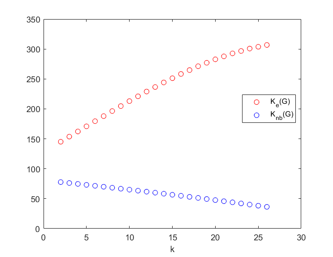
Figure 5: A comparison of the values of $\mathscr{K}_{e}(G)$ and $\mathscr{K}_{nb}(G)$, where $G$ is a cycle barbell of order $n=30$, with $k$ varying from $2$ to $26$, and $a=b=\tfrac{1}{2}(n-k+2)$.

We end with some discussion of open questions and avenues of research. Theorems 5.6 and 5.7 exhibit interesting differences in behavior between a simple random walk and a non-backtracking random walk. For cycle barbells, the simple random walk Kemeny’s constant is largest when there was a large path and small cycles, whereas in the non-backtracking random walk Kemeny’s constant was largest when there was a small path with large cycles. Also note that the edge Kemeny’s constant is an order of magnitude larger than the non-backtracking Kemeny’s constant even when both are compared at $G=CB(2,n/2,n/2)$ (the maximizer for the non-backtracking walk, and minimizer for the simple walk); see Figure 5. In particular $\mathscr{K}_{nb}(G)=O(n)$ and $\mathscr{K}_{e}(G)=O(n^{2})$. This suggests that, while long paths will tend to lead to a large Kemeny’s constant for the simple walk, large cycles make more of a difference for the non-backtracking walk. It would be interesting to further investigate more generally what graph properties lead to large or small simple walk Kemeny’s constant versus a large non-backtracking walk Kemeny’s constant.

Note that from Theorem 3.4, for regular graphs, the simple walk and non-backtracking walk Kemeny’s constants have the same order of magnitude. It is an interesting open question to determine for what graphs these orders of magnitude will be the same, and for what graphs they are different, and by how much they can differ. Moreover, it is known that for the simple walk Kemeny’s constant on the vertices, Kemeny’s constant is at most on the order of $O(n^{3})$ where $n$ is the number of vertices, and there are examples where this order of magnitude is achieved (see [5]). In all examples from this work, the largest non-backtracking Kemeny’s constant that we have seen is on the order of $O(n^{2})$ (but again, the comparison based on size of the graph is a more subtle matter since the state space of the Markov chain is now the number of directed edges). It would be of interest to determine if this is the largest possible order of magnitude.

Finally, in nearly all results from this paper, the non-backtracking Kemeny’s constant is smaller than the simple edge Kemeny’s constant. The only exceptions to this have only a few vertices. Indeed, we have done computations on all connected graphs with minimum degree at least 2 that are not cycles on up to 10 vertices. We have found that for $n=4$ vertices there are 2 graphs with $\mathscr{K}_{nb}(G)\geq\mathscr{K}_{e}(G)$, on $n=5$ vertices there are 10 graphs with $\mathscr{K}_{nb}(G)\geq\mathscr{K}_{e}(G)$, on $n=6$ vertices there are 18 graphs with $\mathscr{K}_{nb}(G)\geq\mathscr{K}_{e}(G)$, on $n=7$ vertices there are 7 graphs with $\mathscr{K}_{nb}(G)\geq\mathscr{K}_{e}(G)$, on $n=8$ vertices there are 3 graphs with $\mathscr{K}_{nb}(G)\geq\mathscr{K}_{e}(G)$, and on $n=9$ and $n=10$ vertices, there are no graphs with $\mathscr{K}_{nb}(G)\geq\mathscr{K}_{e}(G)$. We conjecture that, for all graphs with sufficiently many vertices, the non-backtracking Kemeny’s constant will be smaller.

References

• [1] David Aldous and James Allen Fill. Reversible Markov Chains and Random Walks on Graphs, 2002. Unfinished monograph, recompiled 2014, available at http://www.stat.berkeley.edu/~aldous/RWG/book.html.
• [2] Noga Alon, Itai Benjamini, Eyal Lubetzky, and Sasha Sodin. Non-backtracking random walks mix faster. Communications in Contemporary Mathematics, 9(04):585–603, 2007.
• [3] Francesca Arrigo, Desmond J Higham, and Vanni Noferini. Non-backtracking PageRank. Journal of Scientific Computing, 80(3):1419–1437, 2019.
• [4] Ravindra B Bapat. Graphs and Matrices, volume 27. Springer, 2010.
• [5] Jane Breen, Steve Butler, Nicklas Day, Colt DeArmond, Kate Lorenzen, Haoyang Qian, and Jacob Riesen. Computing Kemeny’s constant for a barbell graph. The Electronic Journal of Linear Algebra, 35:583–598, 2019.
• [6] Lorenzo Ciardo, Geir Dahl, and Steve Kirkland. On Kemeny’s constant for trees with fixed order and diameter. Linear and Multilinear Algebra, pages 1–23, 2020.
• [7] Nolan Faught, Mark Kempton, and Adam Knudson. A 1-separation formula for the graph Kemeny constant and Braess edges. Journal of Mathematical Chemistry, pages 1–21, 2021.
• [8] Cory Glover and Mark Kempton. Some spectral properties of the non-backtracking matrix of a graph. Linear Algebra and its Applications, 618:37–57, 2021.
• [9] Roger A Horn and Charles R Johnson. Matrix Analysis. Cambridge University Press, 2012.
• [10] Jeffrey J Hunter. Mixing times with applications to perturbed Markov chains. Linear Algebra and its Applications, 417(1):108–123, 2006.
• [11] Mark Kempton. Non-Backtracking Random Walks and a Weighted Ihara’s Theorem. Open Journal of Discrete Mathematics, 6(4):207–226, 2016.
• [12] Mark Kempton. A non-backtracking Pólya’s theorem. J. Comb., 9(2):327–343, 2018.
• [13] Florent Krzakala, Cristopher Moore, Elchanan Mossel, Joe Neeman, Allan Sly, Lenka Zdeborová, and Pan Zhang. Spectral redemption in clustering sparse networks. Proceedings of the National Academy of Sciences, 110(52):20935–20940, 2013.
• [14] Mark Levene and George Loizou. Kemeny’s constant and the random surfer. The American mathematical monthly, 109(8):741–745, 2002.
• [15] José Luis Palacios and José M Renom. Broder and Karlin’s formula for hitting times and the Kirchhoff index. International Journal of Quantum Chemistry, 111(1):35–39, 2011.
• [16] Rushabh Patel, Pushkarini Agharkar, and Francesco Bullo. Robotic surveillance and Markov chains with minimal weighted Kemeny constant. IEEE Transactions on Automatic Control, 60(12):3156–3167, 2015.
• [17] Leo Torres, Kevin S Chan, Hanghang Tong, and Tina Eliassi-Rad. Nonbacktracking eigenvalues under node removal: X-centrality and targeted immunization. SIAM J. Math. Data Sci., 3(2):656–675, 2021.
• [18] Serife Yilmaz, Ekaterina Dudkina, Michelangelo Bin, Emanuele Crisostomi, Pietro Ferraro, Roderick Murray-Smith, Thomas Parisini, Lewi Stone, and Robert Shorten. Kemeny-based testing for COVID-19. Plos one, 15(11):e0242401, 2020.